Maier, Chapter 14: Assorted Topics

Chapter 14

ASSORTED TOPICS

This chapter examines further topics in dependency theory, some limitations of relational algebra, and an extension of the relational model to include computed relations.

14.1 LOGIC AND DATA DEPENDENCIES

In this chapter we establish a connection between the theory of FDs and MVDs and a fragment of propositional logic. We give a way to interpret FDs and MVDs as formulas in propositional logic. For a set of dependencies C and a single FD or MVD c, we show that C implies c as dependencies if and only if C implies c under the logic interpretation. We first prove this result when C is FDs alone. We then extend the results to include MVDs, which complicates the proofs of the results considerably.

The correspondence between FDs and propositional formulas is direct. Let X- Y be an FD, where

and

Y = B1 B2 -.- B,.

The corresponding logical formula is

The A’s and B’s are viewed as propositional variables. The shorthand we use for this logical formula is X =$ Y. If X or Y is empty, we use true in place of

485

486 Assorted Topics

the conjunction of variables. Thus, the corresponding logical formula for X- YwhenX= @is

There is some easy evidence that this correspondence of FDs and formulas will give the desired equivalence of FD implication and logical implication: all the inference rules for FDs are valid inference rules for logic when the FDs are interpreted as logical formulas (see Exercise 14.1).

Example 14.1 Consider the transitivity rule for FDs:

X-Y and Y+Z imply X + Z.

The corresponding rule for logical inference is

X 3 Y and Y * Z imply X 3 Z,

which is the transitive rule of inference for logic. If we know A B + C and C 4 D E, we may conclude A B + D E. Likewise, if we know A A B * C and C * DAE, wemayinferA AB *D AE.

14.1.1 The World of Two-Tuple Relations

In the rest of the material on dependencies and logic, we shall make extensive use of relations with only two tuples. By the world of two-tuple relations we mean dependency theory restricted to relations consisting of exactly two tuples. For FDs and MVDs, we shall see that implication in the world of two- tuple relations is the same as implication over unrestricted (finite) relations. The equivalence does not hold for IDS or embedded MVDs.

Let r be a relation over scheme R with exactly two tuples. Call them tl and t2. Relation r can be used to define a truth assignment for the attributes in R, when they are considered as propositional variables.

Definition 14.1 Let r be a relation on scheme R. The truth assignment for r, denoted %‘r, is the function from R to {true, false} defined by

if tl(A) = t2(A) *,(A) =

ift,(A) # t2(A).

Logic and Data Dependencies 487

Example 14.2 Let r(A B C D) be the relation in Figure 14.1. The truth assignment for r is given by

$,(A) = t7-m *JB) = false q,(C) = false yk,(D) = true.

r(A B C D)

1 2 4 6 1 3 5 6

Figure 14.1

Lemma 14.1 Let X ---, Y be an FD over R and let r be a relation on R with two tuples, tl and t2. X + Y is satisfied by r if and only if X =r Y is true under the truth assignment 9,.

Proof (if) Let X = Al A2 - * - A, and let Y = B1 B2 - n. B,. If ‘k, makes X* Ytrue,then9,mustmakeA,~A~~-~~AA,falseorB~~B~~~~~~ B, true. IfA AA2 A -es A A, is false, then for some i between 1 and m we have t,(Xi) f t2(Xi). It follows that r satisfiesx + Y. If B1 A B2 A - - - A B, is made true by P,, then tl( Y) = t2( Y), and so X -+ Y is again satisfied.

(only if) Left to the reader (see Exercise 14.3).

Example 14.3 Let r(A B C D) be the relation from the last example. The FDA - D is satisfied by r, and P, makes A * D true. Relation r does not satisfy A - B, and \k, makes A * B false.

Lemma 14.2 Let r(R) be a relation, let F be a set of FDs on R, and let X --, Y be a single FD on R. If r satisfies F and violates X + Y, then some two-tuple subrelation s of r satisfies F and violates X + Y.

Proof The result is fairly immediate, and we do not include a proof. We only recall that if T satisfies F, so does any subrelation of r.

Example 14.4 Figure 14.2 shows a relation r on scheme A B C D that satisfies the set of FDs F = {AB -+ D, C + D } and violates C 4 B. Figure 14.3 shows a two-tuple subrelation s of r that satisfies F and violates C --, B.

488 Assorted Topics

rfA I3 C D)

1 2 4 6 1 2 5 6 1 3 5 6 1 3 4 6

Figure 14.2

s(A B C D)

1 2 5 6 1 3 5 6

Figure 14.3

There is a certain set of two-tuple relations that we shall need in the proof of the next theorem. Let R be a relation scheme and let X c R. We let 2x stand for the relation on R that consists of two tuples, tl and tZ, where tl is all l’s and t2 is l’s on X and O’s elsewhere. The important point is that 2, is a two-tuple relation where the tuples agree on exactly X.

Example 14.5 Figure 14.4 shows the relation 2* on scheme A B C D.

2,&A B C D)

1 1 1 1 1 1 0 0

Figure 14.4

14.1.2 Equivalence of Implication for Logic and Functional Dependencies

Theorem 14.1 Let P be a set of FDs over scheme R and let X + Y be an FD over R. The following are equivalent.

1. F implies X + Y. 2. F implies X -+ Y in the world of two-tuple relations. 3. F implies X * Y as logical formulas.


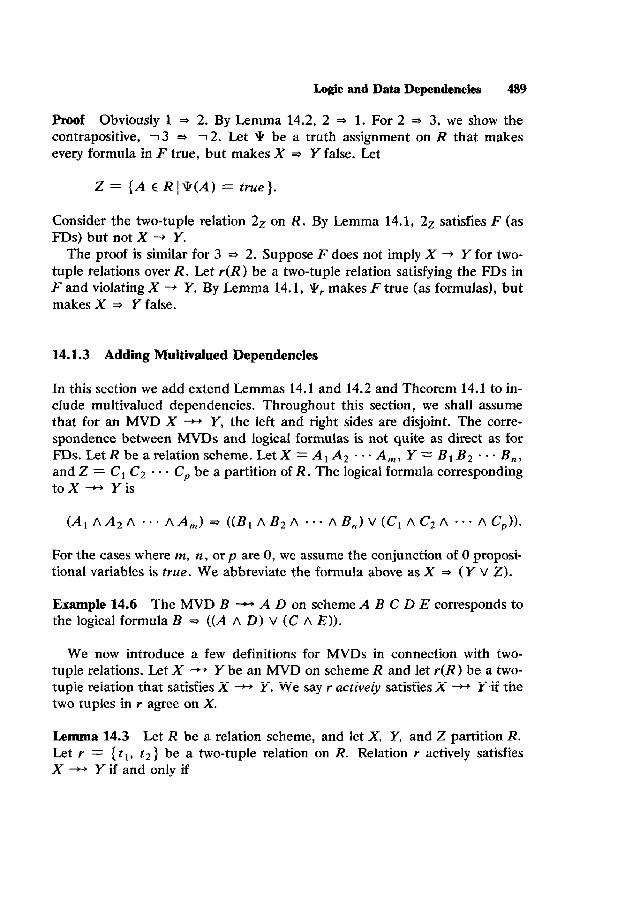
Proof Obviously 1 * 2. By Lemma 14.2, 2 * 1. For 2 * 3, we show the contrapositive, 13 r) -12. Let !P be a truth assignment on R that makes every formula in F true, but makes X * Y false. Let

Consider the two-tuple relation 2z on R. By Lemma 14.1, 2z satisfies F (as FDs) but not X -+ Y.

The proof is similar for 3 * 2. Suppose F does not imply X + Y for two- tuple relations over R. Let r(R) be a two-tuple relation satisfying the FDs in I; and violating X -+ Y. By Lemma 14.1, q’r makes F true (as formulas), but makes X * Y false.

14.1.3 AdCmg Multivalued Dependencies

In this section we add extend Lemmas 14.1 and 14.2 and Theorem 14.1 to include multivalued dependencies. Throughout this section, we shall assume that for an MVD X +-+ Y, the left and right sides are disjoint. The correspondence between MVDs and logical formulas is not quite as direct as for FD~.LetRbearelationscheme.LetX=AiA~+.~A,, Y=BIBZ.--B,, andZ= C, Cz -.* C, be a partition of R. The logical formula corresponding to X -++ Y is

(A,AA,A . . . AA,) 3 ((B1/\B2~ -~~AB,)V(C,AC2A -AC,)).

For the cases where m, IE, or p are 0, we assume the conjunction of 0 propositional variables is true. We abbreviate the formula above as X * (Y v 2).

Example 14.6 The MVD B --H A D on scheme A B C D E corresponds to the logical formula B = ((A A D) v (C A I?)).

We now introduce a few definitions for MVDs in connection with two- tuple relations. Let X - Y be an MVD on scheme R and let r(R) be a two- tuple relation that satisfies X - Y. We say r actively satisfies X ++ Yif the two tuples in r agree on X.

Lemma 14.3 Let R be a relation scheme, and let X, Y, and Z partition R. Let r = ( t,, t2 > be a two-tuple relation on R. Relation I actively satisfies X -++ Y if and only if

I .s: -_ -;:..

490 Assorted Topics

1. tl(X) = tz(X), and 2. t,(Y) = tz(Y) or t,(Z) = t2(Z).

Proof Left to the reader (see Exercise 14.5).

We now give the analogue of Lemma 14.1 with MVDs added.

Lemma 14.4 Let c be an FD or MVD over scheme R and let Y be a two-tupie relation on R. The dependency c is satisfied by I if and only if c as a logical formula is true under the truth assignment qr.

Proof Let r = {tr, t2). If c is an FD, we may appeal to Lemma 14.1, so let c betheMVDX* Y,andletZ=R -XY.

(if) Q, makesX * (Y V Z) true. If \k, makesxfalse, then t,(X) z tZ(X) in P-. Thus r satisfies X - Y. If qk, makes X true, it must also make Y true or Z true. It follows that t,(X) = tZ(X) and either tr(Y) = tz(Y) or t,(Z) = tz(Z). Hence, by Lemma 14.3, X + Y is satisfied.

(only if} Suppose r satisfies X --H Y. If t,(X) # tZ(X), then 9, makesX false, and hence makes X * (Y v Z) true. If tl(X) = t*(X), then r actively satisfiesx - Y. I3y Lemma 14.3, tl( Y) = tz( Y) or t,(Z) = t&Z). It follows that P, makes Y true or Z true, so \k, makes X =j (Y v Z) true.

Lemma 14.5 Let r = { tl, t2] and s = { ul, ~2 ] be two-tuple relations over scheme R. Suppose for every attribute A E R, t,(A) = t*(A) implies z.tl(A) = u2(A). If X --w Y holds actively in r, it also holds actively in S.

Proof Left as Exercise 14.4.

The next lemma is the anaiogue of Lemma 14.2 with MVDs added. The proof is more complex than that for Lemma 14.2, since it is not the case that any subrelation of a relation satisfying an MVD also satisfies the MVD.

Lemma 14.6 Let r be a relation on scheme R, let C be a set of FDs and MVDs on R, and let c be a single FD or MVD on R. If I satisfies C and violates c, then some two-tuple subrelation s of r satisfies C and violates c.

Proof Case 1 (c is an FD) Assume that c is X ---, A. (Why is it permissible to assume that c has a single attribute on the right side?) By Lemma 14.2, there is at least one two-tuple subrelation of I that violates X + A. Let s be one such relation, chosen to actively satisfy as many MVDs in C as any other such subrelation.


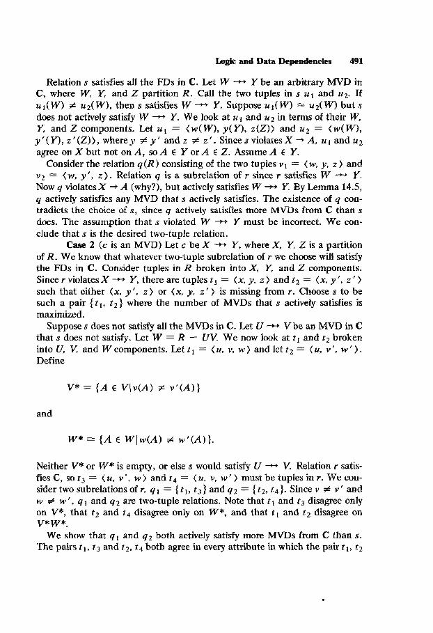
Relation s satisfies all the FDs in C. Let W --H Y be an arbitrary MVD in C, where W, Y, and Z partition R. Call the two tuples in s u1 and ~2. If ul(W) f UZ( W), then s satisfies W - Y. Suppose ul( W) = UZ( W) but s does not actively satisfy W -++ Y. We look at u 1 and ~2 in terms of their W, K and Z components. Let u 1 = (w(W), y(Y), z(Z)) and ~2 = (w(W), y’(y), z’(Z)), wherey # y’ andz f z’. Since s violatesx -+ A, ~1 and 1.9 agree on X but not on A, so A E Y or A E Z. Assume A E Y.

Consider the relation q(R) consisting of the two tuples v1 = (w, y, z ) and v2 = <w, y', z > . Relation q is a subrelation of r since r satisfies W +-+ Y. Now q violatesx --f A (why?), but actively satisfies W --H Y. By Lemma 14.5, q actively satisfies any MVD that s actively satisfies. The existence of q con- tradicts the choice of s, since q actively satisfies more MVDs from C than s does. The assumption that s violated W --f) Y must be incorrect. We conclude that s is the desired two-tuple relation.

Case2 (cisanMVD)L.etcbeX --H Y, where X, Y, Z is a partition of R. We know that whatever two-tuple subrelation of r we choose will satisfy the FDs in C. Consider tuples in R broken into X, Y, and Z components. Since r violates X --H Y, there are tuples tl = (x, y, z > and t2 = (x, y ‘, z’ > such that either (x, y’, z > or (x, y, z ’ > is missing from r. Choose s to be such a pair {tl, t2 } where the number of MVDs that s actively satisfies is maximized.

Suppose s does not satisfy all the MVDs in C. Let U --w Vbe an MVD in C that s does not satisfy. Let W = R - UV. We now iook at tl and t2 broken into U, V, and W components. Let tI = (u, v, w > and let t2 = (u, v’, w ’ >. Define

V” = {A E b+(A) # v’(A))

and

W” = {A E W(w(A) # w’(A)).

Neither V* or W* is empty, or else s would satisfy U - V. Relation r satis- fiesC, sot3 = (u, v’, w> andt, = (u, v, w’) mustbetuplesinr. Wecon- sider two subrelations of r, q1 = { tl, t3) and q2 = { t2, t4). Since v # v’ and w # w ’ , q 1 and q2 are two-tuple relations. Note that t 1 and t3 disagree only on V*, that t2 and t4 disagree only on W*, and that t 1 and t2 disagree on VW”.

We show that q1 and q2 both actively satisfy more MVDs from C than s. The pairs tl, t3 and t2, t4 both agree in every attribute in which the pair tl, t2

492 Assorted Topics

agrees. Thus, by Lemma 14.5, q i and q2 actively satisfy every MVD that s actively satisfies. Further, q1 and q2 both actively satisfy U --H V.

If either q I or q2 violates X -++ Y, we are done, for we then have a contradiction to the choice of s. Suppose q I and q2 both satisfy X --w Y. They both must then actively satisfy X --tt Y, since tl, t2, t3, and t4 all have the same X-value. By Lemma 14.3, since q1 actively satisfies X - Y, ti and t3 agree on X, and they also agree on either Y or Z. If they agree on Y, then V* C Z, since tl and t3 only disagree on V *. If tl and t3 agree on Z, then V* 5 Y. A similar argument on q2 shows that W* C Z or W* G Y.

If V* G Y and W* E Y, then tl and t2 agree on all of Z, which means s satisfies X - Y. Thus, that combination of containments cannot hold. Sim- ilarly, V* E Z and W* E Z cannot hold simultaneously. The only remaining possibility for the combination is V * E Y and W* G Z, or V* E Z and W* C Y. By symmetry, we only examine the first possibility, We have t3 = (x, y’, Z> and t4 = (x, y, z’}. One of (x, y’, z) and (x, y, z’} was assumed missing from r in the construction of s, but t3 and t4 are both sup- posed to be in 1. We have a contradiction to the supposition that q1 and q2 satisfy X --f) Y.

We conclude that at least one of q1 and q2 violates X -++ Y, which contra- dicts the choice of s. Our assumption that s violated some MVD in C must have been incorrect, so s is the desired two-tuple relation.

Theorem 14.2 Let C be a set of FDs and MVDs over scheme R and let c be a single FD or MVD over r. The following conditions are equivalent.

1. C implies c. 2. C implies c in the world of two-tuple relations. 3. C implies c when dependencies are interpreted as logical formulas.

Proof The proof is similar to that of Theorem 14.1. Lemmas 14.4 and 14.6 take the place of Lemmas 14.1 and 14.2. The details are left to the reader (see Exercise 14.7).

14.1.4 Nonextendibility of Results

The correspondence between logic and data dependencies cannot be extended to include JDs or embedded MVDs. This limitation is not too suprising when we note that implication for these types of dependencies is not the same in the world of two-tuple relations as it is for regular relations (see Exercise 14.9).

More Data Dependencies 493

We show that no extension of our correspondence works for IDS; the corresponding proof for EMVDs is left as Exercise 14.10.

Suppose the correspondence between logic and data dependencies extended to IDS. Consider the ID *[A& BC, AC]. Suppose that this ID has a corresponding logical formulaf, Since *[A& BC, AC] follows from A --f+ B, A * (B V C) should imply f. Likewise, considering B --H C, B * (A V C) should imply f. Consider any truth assignment * for {A, B, C). If 9(A) = false, then \E makes A * (B V C) true, and so q makes f true. If 3(A) = true, then @ makes B * (A v C) true, so it also makes f true. Formula f must be a tautology, since every truth assignment makes it true. However, *[AB, BC, AC] does not always hold. We were in error assuming *[A& BC, AC] has a corresponding logical formula that is consistent with the logical interpretation that we gave to MVDs.

14.2 MORE DATA DEPENDENCIES

Why do we need more types of data dependencies? Are not FDs, MVDs, IDS and their embedded versions enough? There is some evidence that these dependencies do not form a natural class, that there is something missing. The class of sets of instances definable with FDs, MVDs, and IDS is not closed under projection. In Section 9.3 we saw that for a set F of FDs over scheme R, nx(SAT(F)) cannot be described always as SAT(F) for a set F’ of FDs over X. We saw that a similar remark holds for MVDs. The remark also applies to IDS (see Exercise 14.11). Another problem is that there are no complete sets of inference axioms for embedded MVDs, and there is no known complete set of inference axioms for IDS. It has been shown that no such set of axioms exists for EMVDs, and there is evidence that no such rules exist for IDS. (See Bibliography and Comments at the end of this chapter.) While we do have the chase for determining implication of IDS, the fast implication algorithms for FDs and MVDs are based on inference axioms and not the chase. Also, the chase is an unwieldy tool for generating al dependencies of a given type that are implied by a set of dependencies.

The hope in studying larger classes of data dependencies is that a more general class will be found that contains FDs and IDS, and also avoids the problems mentioned above. Template dependencies and generalized functional dependencies are attempts to find such a class of more general dependencies. Template dependencies generalize IDS, and generalized functional dependencies generalize (you guessed it) FDs. These more general dependencies handle the first problem above. Sets of instances defined by satisfaction of these dependencies are closed under projection, as we shall see. These

494 Assorted Topics

generalized dependencies do not do quite as well in solving the inference axiom problem. A complete set of inference axioms exists for template dependencies, but only for “infinite implication.” That is, the axioms are complete for reasoning about implication in situations where relations are allowed to be infinite. We shall see that the inference axioms are not complete for implication where relations are restricted to be finite. We shall also see that there are an infinite number of inequivalent template dependencies over schemes of sufficiently large size, so it is generally not possible to generate all the template dependencies implied by a set of template dependencies.

The chase computation can be extended to template dependencies with a few modifications, but the tableaux that result from chasing with template dependencies can be infinite. Even though we are guaranteed to generate the “winning row” in the chase after a finite amount of time (if an implication holds), the chase cannot serve as a basis for a decision procedure for template dependency implication. One might imagine a decision procedure that simultaneously runs the chase to test a given implication and looks for counterexamples to the implication. This plan fails because there can be an infinite counterexample to a relation but no finite counterexample. It is not likely that any modification of this plan will work, for the implication problem has been shown undecidable for a slight generalization of template dependencies.

There are some subcases of the implication problem for template dependencies that are decidable. One is where we seek only implication by a single template dependency. Another case is where the template dependencies are not embedded. In both cases the chase computation terminates. In the latter case, the chase computation terminates even when generalized functional dependencies are added.

14.2.1 Template Dependencies

A template dependency is essentially a statement that a relation is invariant under a certain tableau mapping. When written down, a template dependency looks like a tableau with a special row at the bottom, somewhat like an upside-down tableau query. The special row is called the concfusi~n row; the other rows are the hypothesis rows. For a relation r to satisfy a template dependency, whenever there is a valuation p that maps the hypothesis rows to tuples in r, p also must map the conclusion row to a tuple in r. There is a slight complication to this informal definition, to handle variables in the conclusion row that do not appear in the hypothesis rows.

Example 14.7 Figure 14.5 shows a template dependency T over scheme A B C. The hypothesis rows are w ,-w4; w is the conclusion row. Relation I in Figure


14.6 does not satisfy 7, since the valuation p that maps wi to ti, 1 I i 5 4, does not map w to any tuple in r. Adding a tuple t5 = (1 3 6) to r makes r satisfy r, although this fact is tedious to check.

?(A B C)

wla b c’ wza b’ c’ w3a b’ c wqa’ b c

wa b c

Figure 14.5

r(A B C) t,l 3 5 t*l 4 5 tgl 4 6 td2 3 6

Figure 14.6

We now provide a formal definition for a template dependency and its satisfaction. While template dependencies are not exactly the same as tableaux, they are sufficiently similar so that tableau concepts, such as valuation and containment mapping, apply to the set of hypothesis rows in a template dependency. In the following definition, when we refer to a row over scheme R, we mean a tuple of abstract symbols or variables, as in tableaux. We do not make the distinguished-nondistinguished distinction on variables that we did with tableaux, however.

Definition 14.2 A template dependency (TD) on a relation scheme R is a pair7=(T,w)whereT={w1,w2, . . . . wk } is a set of rows on R, called the hypothesis rows, and w is a single row on R, called the conclusion row. A relation r(R) satisfies TD r if for every valuation p of T such that p(T) C r, p can be extended in such a way that p(w) E r. TD T is trivial if it is satisfied by every relation over R.

TDs are written as shown in Figure 14.5, with the conclusion row at the bottom, separated from the hypothesis rows by a line. For variables, we usually use lowercase letters corresponding to the attribute name or symbol, with the unprimed or unsubscripted version appearing in the conclusion row.

4% Assorted Topics

While TDs almost look like tableau mappings turned upside down, there are two differences:

1. A variable in the conclusion row need not appear in any hypothesis row.

2. Variables are not restricted to a single column.

To elaborate on point 1, a TD r on scheme R where every variable in the conclusion row appears in some hypothesis row is calledfull. Let wl, w2, . . . , wk be the hypothesis rows of T and let w be the conclusion row. We say r is S-partial, where S is the set

{A f R (w(A) appears in one of wr, ~2, . . . , wk >.

Naturally, if S = R, then T is full. If S # R, we say r is strictly partial. If r is S-partial, the conclusion row of 7 specifies a tuple with certain values on the attributes in S, but it puts no restriction on the values for attributes in R-S.

Example 14.8 The TD T on A B C in Figure 14.7 is A B-partial.

T(A B C) a’ b’ c’ a’ b c’~ a b’ c”

a b c

Figure 14.7

To elaborate on point 2, a TD where each variable appears in exactly one column is called a typed TD. If some variable appears in multiple columns, the TD is called untyped. The TDs in Figures 14.5 and 14.7 are typed. For the rest of our treatment of template dependencies, we shall assume that all TDs are typed, unless they are explicitly said to be untyped.

ExampIe 14.9 Figure 14.8 shows an untyped TD T. This TD assumes that dam(A) = dam(B) and asserts that a relation is transitively closed (when considered as a binary relation in the mathematical sense).


a b b c

a c

Figure 14.8

Any join dependency, full or embedded, can be represented as a TD (see Exercise 14.15).

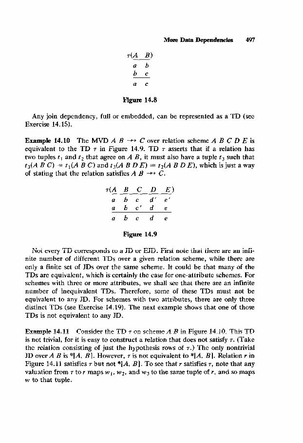
Example 14.10 The MVD A B -+ C over relation scheme A B C D E is equivalent to the TD 7 in Figure 14.9. TD T asserts that if a relation has two tuples tl and t2 that agree on A B, it must also have a tuple t3 such that tj(A B C) = tl(A B C) and tj(A B DE) = t2(A B DE), which is just a way of stating that the relation satisfies A B - C.

7(A B C D E)

a b c d’ e’ a b c’ d e

abc de

Figure 14.9

Not every TD corresponds to a JD or EJD. First note that there are an infinite number of different TDs over a given relation scheme, while there are only a finite set of IDS over the same scheme. It could be that many of the TDs are equivalent, which is certainly the case for one-attribute schemes. For schemes with three or more attributes, we shall see that there are an infinite number of inequivalent TDs. Therefore, some of these TDs must not be equivalent to any JD. For schemes with two attributes, there are only three distinct TDs (see Exercise 14.19). The next example shows that one of those TDs is not equivalent to any JD.

Example 14.11 Consider the TD 7 on scheme A B in Figure 14.10. This TD is not trivial, for it is easy to construct a relation that does not satisfy T. (Take the relation consisting of just the hypothesis rows of 7.) The only nontrivial JD over A B is *[A, B]. However, 7 is not equivalent to *[A, B]. Relation r in Figure 14.11 satisfies 7 but not *[A, B]. To see that r satisfies 7, note that any valuation from 7 to r maps wl, w2, and w3 to the same tuple of I, and so maps w to that tuple.

498 Assort& Topics

W B 1 w1 a b’ w2 U’ b’ w3 a’ b

w a b

Figure 14.10

r(A B) 1 3 2 4

Figure 14.11

14.2.2 Examples and Counterexamples for Template Dependencies

In this section we see that there is a strongest TD over any scheme, as well as a weakest, nontrivial, full TD. We shall also exhibit a relation that obeys every strictly partial TD, but violates every full TD, thus showing that a set of strictly partial TDs cannot imply a nontrivial full TD.

Theorem 14.3 For any relation scheme R, there is a strongest TD r on R. That is, any relation r(R) that satisfies r also satisfies any other TD T’ on R.

Proof The TD r we want states that a relation is a column-wise Cartesian product. For example, on the scheme A I3 C D, the Cartesian product TD is shown in Figure 14.12. Any relation that is a Cartesian product satisfies every TD (see Exercise 14.21).

a bl ~1 dl al b ~2 d2 a2 b2 c d3 a3 b3 ~3 d a b c d

Figure 14.12


While there is no weakest nontrivial TD in general (see Exercise 14.22b), there is a weakest full TD on any scheme with 2 or more attributes. Note that there are only trivial TDs over a scheme with a single attribute.

Theorem 14.4 For any relation scheme R with two or more attributes, there is a weakest nontrivial full TD r on R. That is, if r’ is another nontrivial full TD on R, any relation r(R) that satisfies 7’ also satisfies ‘T.

Proof Assume R = Al A2 se+ A,, where n 1 2. For each Ai, 7 has two variables in the Aj-column, ai and bj. Let r = (T, w), where T contains every possible row of u’s and b’s, except the row of all u’s The conclusion row, w, is the row of all a’s. Figure 14.13 shows TD T when R = Al A2 A3.

Let r ’ = (T’ , w ’ ) be another nontrivial full TD over R. The conclusion row w’ cannot appear in T’ (see Exercise 14.23). We show that 7’ is stronger than r by exhibiting a containment mapping $ from r’ to r. That is, $ maps variables in 7’ to variables in r in such a way that $( T’) C T and $(w’) = w. Thus, for any relation r(R) and for any valuation mapping p on T such that p(T) c r, p’ = p 0 II/ is a valuation mapping for T’ such that p’( T’) E 1: If Y satisfies r ‘, then r contains p’(w ’ ), which is the same as p(w), so r satisfies r.

For ease of notation while dealing with $, assume that the variables in 7’ are renamed so that w = w ’ . For the A;-column of r ’ , let 1c/ map a; to ai, and let it map any other variable to bi. Clearly, $(w ‘) = w. For any hypothesis row v of T’, +(v) will be a row of u’s and b’s (other than the row of all a’s), so $(v) E T. Therefore $(T’) E T, and we are finished.

dAt A2 A31

bl b2 b3 bl bz ~3

bl a2 b3 bl ~2 ~3

~1 b2 b3 a1 b2 a3

al a2 b3 a1 a2 a3

Figure 14.13

Theorem 14.5 Let R be a relation scheme, and let C be a set of strictly partial TDs over R. C does not imply any nontrivial full TD over R.

500 Assorted Topics

Proof L&R =A,A2 -. - A,. Consider the relation r(R) that contains all tuples of rz O’s and l’s, except the row of all 1’s. Figure 14.14 shows r for R = A 1 AZ A3. Since the projection of r onto any proper subset of R is a Car- tesian product relation, r satisfies every strictly partial TD. However, r violates the weakest nontrivial full TD, constructed in the proof of Theorem 14.3. The valuation p that maps ai to 1 and bi to 0, 1 5 i I II, maps the weakest TD into r, but p cannot be extended to the row of all a’s. It follows that r violates any nontrivial full TD over R, and so r serves as a counterexample to any proposed implication of a full nontrivial TD by C.

r(A, A2 Ad

0 0 0 0 0 1 0 1 0 0 1 1 1 0 0 1 0 1 1 1 0

Figure 14.14

14.2.3 A Graphical Representation for Template Dependencies

Testing whether or not a relation r satisfies a TD r is a tedious task at best, since it involves finding all valuations from the hypothesis rows of r into the tuples of r. In this section we introduce a graphical representation for relations and TDs that makes finding such valuations somewhat easier, at least for small examples done by hand. Also, the graphical notation removes some extraneous details, and so gives a more concise method for expressing TDs in most cases.

The actual values in relations and the actual variables in TDs are of no im- portance in testing if a relation satisfies a TD. What is important is equalities among values and among variables. We use undirected graphs to represent relations and TDs. The nodes stand for tuples or rows, as the case may be; labeled edges between nodes indicate where two tuples or rows match.

Definition 14.3 Let r be a relation on scheme R = Al AZ - - - A,, . The graph of r, denoted G,, is an undirected graph with labeled edges constructed as follows. The nodes of G, are the tuples of r. For two tuples tl and 12 in r, there is an edge (t,, t2) in G, exactly when t, and t2 agree on some attribute


in R. The edge (tl, t2) is labeled by the set of attributes on which t1 and t2 agree.

Example 14.12 Let r be the relation in Figure 14.6. Figure 14.15 shows G,, the graph of P. In drawing graphs of relations, we remove any edge from a node to itself (there is such an edge for every node), and sometimes omit edges that can be inferred by transitivity. Thus, we could just as well depict G, as in Figure 14.16.

ABC

ABC

ABC

Figure 14.15

Figure 14.16

The graph for a TD 7, denoted G,, is defined similarly, except that we label the node for the conclusion row with a *.

Example 14.13 If r is the TD from Figure 14.5, then G, is shown in Figure 14.17. Again, we omit self-loops and some edges implicit by transitivity.

502 Assorted Topics

Figure 14.17

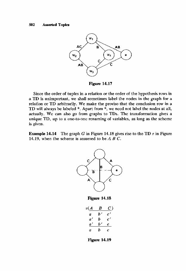
Since the order of tuples in a relation or the order of the hypothesis rows in a TD is unimportant, we shall sometimes label the nodes in the graph for a relation or TD arbitrarily. We make the proviso that the conclusion row in a TD will always be labeled *. Apart from *, we need not label the nodes at all, actually. We can also go from graphs to TDs. The transformation gives a unique TD, up to a one-to-one renaming of variables, as long as the scheme is given.

Example 14.14 The graph G in Figure 14.18 gives rise to the TD r in Figure 14.19, when the scheme is assumed to be A B C.

Figure 14.18

T(A B C) a b’ c’ a’ b c’ a’ b’ c a b c

Figure 14.19


We now define an analogue for valuation in terms of labeled graphs.

Definition 14.4 Let G1 = (Ni, El) and G2 = (&, Ez) be two undirected graphs whose edges are labeied with subsets of some set L. A mapping h : N, + N2 is a label-preserving homomolphkm (Ip-homomorphism) of G1 to Gz if for any edge e = (v, w) in El, if L1 is the label of e and L2 is the label of (h(v), h(w)) in GZ, thenL1 c Lt.

Example 14.15 Let G, be the graph in Figure 14.16 and let G, be the graph in Figure 14.17. The function hi defined as

hlhd = tl h,hd = t2 hl(w& = t2 hl(wd = ti hl(*) = tl

is an Ip-homomorphism from G, to G,. (Recall that there are self-loops for all the nodes in G,, although they are omitted from the figure.) The mapping h2 defined as

hl(wd = $1 hl(w2) = t3

hl(wd = t3

h,(wd = t2

hl(*) = t2

is not an Ip-homomorphism from G, to G,, since, for example, (wi, ~4) has label B in G,, but (h(w,), h(w2)) = (ti, t2) has label A C.

We can express satisfaction of a TD by a relation in terms of lp-homomorphism between their graphs. In the following theorem, G, - {*> means the graph of TD r without the node for * or its connecting edges.

Theorem 14.6 Let r be a relation over scheme R with graph G,. Let r be a TD over R with graph G,. Relation r satisfies r if and only if for any tp-homomorphism h from G, - { *} to G, can be extended to an Ip-homomorphism from all of G, to G,.


504 Assorted Topics

Example 14.16 Let G, be the graph in Figure 14.16 and let G, be the graph in Figure 14.17. (The same graphs as in the last example.) The mapping h defined as

h(w) = t1

h(w,) = t2 h(w3) = t3

h(W4) = 64

is an lp-homomorphism from G, - { *} to G,. Any extension of h to all of G, is not an lp-homomorphism. Suppose we extend h so that h(*) = t4. This extension is not an Ip-homomorphism since (w4, *) has label A B in G,, but (h(w,), h(*)) = (t,, t4) has only label A in G,.

We now give an application of graphical representation of TDs in proving that there are an infinite number of inequivalent full TDs over a scheme of three attributes. We first need the following lemma, which also is proved with the use of graphical representations.

Lemma 14.7 Let 7 be a TD over relation scheme R. Let w ’ be a row over R such that if w ’ mentions any variable in the conclusion row of 7, some hypothesis row of 7 also contains that variable. Form TD 7’ by adding w ’ to the hypothesis rows of 7. Then 7 implies 7’.

Proof By the choice of w ’ , we can draw the graph G,’ as G, with a node w ’ added such that no edges connect w ’ and *. Consider an arbitrary relation r(R). Any lp-homomorphism h’ from G,’ - f *} to G, can be restricted to an lp-homomorphism h from G, - { *} to G,. If r satisfies 7, then h can be extended to all of G,. By the form of the graph G,I , h ’ can therefore be extended to all of G, I. Hence, if r satisfies 7, it also satisfies 7’.

Theorem 14.7 (progressively weaker chain) There is an infinite sequence 71,

72, 739 * * * of full TDs such that 7i implies 7i+1 for i L 1 and no two TDs in the sequence are equivalent.

Proof Consider the infinite graph G in Figure 14.20. For i 1 1, let Gi be the sub-graph of G on nodes { *, 1, 2, . . . , i -I- 1) and let 7i be the TD corresponding to Gi. By Lemma 14.7, we have that 7i implies Tit-1 for i 1 1. To complete this proof, we need only show that no pair 7;, T;+~ of consecutive TDs are equivalent. We do so by exhibiting a relation r that violates 7; but satisfies 7i+ 1.


We construct Y by treating the hypothesis rows of ri as a relation. Note that the graph G, for r is just G restricted to the nodes { 1, 2, . . . , i -I- 1). Relation T is easily seen to violate ri. The mapping h defied as h 0’ ) = j for 1 I i s i -I- 1 is an lp-homomorphism from Gi - { *} to G, that cannot be extended to 0.

We now must show that I satisfies ri+l. Let h be an arbitrary Ip-homomorphism from Gi+ I - { *} to G,. We prove that h can be extended to all of G i+l. Since Gi+l - { *) has one more node than G,, h must map two nodes of Gi+l - { *> to the same node of G,. Suppose an odd-numbered node m and an even-numbered node n of Gi+ 1 - { * ) get mapped to the same node of G,. Node m agrees on A with all odd-numbered nodes of Gj+l - { *) and n agrees on A with all even-nulnbered nodes. Since h(m) = h(n), h(j) must agree with h(k) on A for any nodesj and k in Gj+t - (*}. In particular, h(l) and h(2) agree on A, so h can be extended to Gi+i by letting h(*) = h(2).

We now show that a contradiction arises if we assume that h never maps an odd-numbered node and an even-numbered node of Gi+i - (*} to the same node in G,. Let h(1) = j. Consider the case wherej is odd. Since h(2) must agree with h(1) on B and we assume h(1) # h(2), h(2) is forced to be j f 1. For h(3), since h(2) and h(3) must agree on C, but h(2) # h(3), we must have k(3) = j + 2. Continuing in this manner, we see that h(k) = j i- k - 1 for lrk5i+2.However,wemustthenhaveh(i+2)=j+i+l>i+2, which cannot happen since i + 1 is the largest-numbered node in G,.

In the case wherej is even, we can show that h(k) = j - k -I- 1 by a similar argument. We again run into a contradiction, since we must then have h(i + 2) = j - i - 1, which is less than 1 because j is no larger than i i- 1.

We see that h can always be extended to Gi+,. Hence, ri+i satisfies r, and we have shown Ti and ri+l inequivalent.

A A A

A A

Figure 14.20

506 Assorted Topics

14.2.4 Testing Implication of Template Dependencies

In this section we take a short look at problems that arise in computing implications of TDs. The first problem is that certain implications holding for finite relations do not hold when relations are allowed to be infinite. Thus, it is unlikely that a complete set of TD inference axioms exists for finite relations, although such a set exists for arbitrary relations. The next theorem shows that implication is not the same for finite relations and arbitrary relations. By arbitrary relations we mean relations that may be finite or infinite.

Theorem 14.8 There is a set C of TDs and a single TD 7 such that any finite relation that satisfies C also must satisfy 7, but there is an infinite relation that satisfies C yet violates 7.

Proof The proof is quite long. We sketch the proof here and leave the details to the reader (see Exercise 14.29).

Let c = {71, 72, 739 74) h w ere Ti corresponds to graph Gi, 1 5 i I 4, in Figures 14.21-24. There is a system behind the TDs in C. We interpret the graph G, of a relation Y as a directed graph D,. A subgraph of G, that matches Figure 14.25 is interpreted as the directed edge tl - t3 in D,. TDs 71 and r2 together say that if D, has an edge u - v, then it also has an edge v - w, for some w. That is, every node in D, with an incoming edge also has an outgoing edge. (A node with no incoming edges is called a sink.) TD 73 basically forces D, to be transitively closed. TD 74 comes into play when D, has a self-loop edge u - U. TD 7 corresponds to the graph G in Figure 14.26.

The property from graph theory that is the mechanism behind this proof is that any finite directed graph that is transitively closed and has no sinks must have a self-loop. The property does not hold for infinite graphs. The proof that C implies 7 for finite relations basically mimics the proof of the property from graph theory. First, the existence of an lp-homomorphism from G - { *} to G,, for some relation r, implies an edge in D,. The presence of an edge implies a cycle in D, reachable from the edge, otherwise, some node would be a sink (so r would violate 71 or TV). Once the cycle is established, transitivity (application of r3) provides the self-loop. The self-loop means 74 is applica- ble. The tuple that 74 requires in Y is also the tuple that 7 requires.

The infinite relation that satisfies C but violates 7 is

r = {<iijO>\l 5 i <j} U ((0iii))i 2 11.

. More Data Dependencies 507

A proof by cases shows that Y satisfies each TD in C. However, the lp-homomorphism h from G to G, defined by

A----- h(1) = (0 1 1 1) h(2) = (1120) h(3) = (0 2 2 2) h(4) = (2 2 3 0)

cannot be extended to *, since we would need h(*)(A) = h(*)(D) = 0, and no such tuple exists in r.

Figure 14.21

Figure 14.22

508 Assorted Topics

G3

Figure 14.23

G*

Figure 14.24

Figure 14.25

Mow Data Dependencies 509

G

Figure 14.26

There is a special case where the set of TDs implied by a set C of TDs is the same for finite and arbitrary relations. If all the TDs in C are S-partial for the same S, then if C implies r for finite relations, C implies r for arbitrary relations (see Exercise 14.30). In particular, finite and arbitrary implication are the same for full TDs.

There is a complete set of inference axioms for TDs in arbitrary reiations. The axioms are, of course, correct for finite relations, but not complete, by the last theorem. One inference axiom, called augmentation, is given by the statement of Lemma 14.7. We give another axiom here, but leave the rest of the set and the proof of completeness as Exercises 14.31 and 14.32.

Weakening If r = (T, w) is a TD, and we obtain the row w’ from w by changing some variables in w to variables that do not appear in T, then T implies the TD r’ = (T, w ‘).

To see that weakening is correct, let r be a relation satisfying 7. If p is a valuation such that p(T) E r, then p(w) E r. We can extend p so that p(w ‘) = p(w), since p is unconstrained on any variable in w ’ not in w. Hence, p(w ‘) E r and so r satisfies 7’.

Example 14.17 The TD r in Figure 14.27 implies the TD r’ in Figure 14.28 by weakening,

dA B Cl

a b’ c’ a’ b’ c a’ b c

a b c

Figure 14.27

510 Assorted Topics

7(A B C)

a b’ c’ a’ b’ c a’ b c

a b” c

Figure 14.28

We now look at extending the chase to handle TDs. We want to use a TD 71 = (Tr, wt) to chase the hypothesis rows of a TD 72 = (T2, w2) to see if w2 can be generated. We need a T-rule for chasing with TDs. The definition of the T-rule is straightforward for full TDs.

T-de Let 7 = (T2, w) be a full TD on scheme R and let T2 be a tableau on R. If there exists a valuation p on T1 such that p(T1) E T2, but p(w) is not in T2, add p(w) to T2.

Example 14.18 Let r1 be the TD in Figure 14.29. Let T be the tableau shown in Figure 14.30. To simplify the notation, we shall represent T with just the subscripts of the variables, remembering that the same number stands for different variables in different columns. The simplified version of T is shown in Figure 14.31. Using the valuation p from rl to T such that

pt<a b’ c’)) = (3 3 2) ptta’bc’)) = (233) p((a’ b’ c)) = (2 2 2),

we can apply the T-rule for 71 to T to add the row

~((a b c>) = (3 3 2).

The resulting TD T’ is shown in Figure 14.32.

7164 B C 1

a b’ c’ a’ b c’ a’ b’ c

a b c

Figure 14.29


T(A B C )

QI bz ~3

a3 b2 ~2

a2 b3 ~2 a2 b3 cl a2 b2 ~2

Figure 14.30

T(A B C)

1 2 3 3 2 2 2 3 2 2 3 1 2 2 2

Figure 14.31

T(A B C)

1 2 3 3 2 2 2 3 2 2 3 1 2 2 2 3 3 2

Figure 14.32

A problem arises in extending the T-rule to strictly partial TDs. We have to create new variables in the columns where the conclusion row contains a variable not in any hypothesis row. We extend the T-rule to handle partial TDs.

T-rule (revised) Let 7 = ( T1, w) be an S-partial TD on scheme R, and let T2 be a tableau on R. If there exists a valuation p on T1 such that p(T1) c T2, and there is no row in Tz that matches p(w) on S, then add the row w ’ to T2, where w ’ matches p(w) on S and w’(A) is a new variable for A E R - S.

Example 14.19 Let r2 be the partial TD in Figure 14.33. Using the valuation p from 72 to tableau T in Figure 14.31 where

512 Assorted Topics

,~((a b’ c’)) = (1 2 3) ~((a’ b’ c)) = (3 2 2),

we can apply the T-rule for 72 to add the row (1 4 2) to T.

44 B C )

a b’ c’ a’ b’ c

a b c

Figure 14.33

Since the choice of new variables is arbitrary in the revised T-rule, chasing with partial TDs does not give a unique result. There is little we can do about this problem, and it is not that serious, for we are interested in which combinations of original variables in a tableau get generated during a chase computation. A serious problem is that applying the T-rule can result in an infinite sequence of tableaux where no new combinations of original variables are being generated, but such combinations could be obtained by applying the T-rule in a different manner.

Example 14.20 Let 72 be the TD in Figure 14.33 and let 73 be the TD in Figure 14.34. Say we start chasing the tableau T in Figure 14.35 (again we show only subscripts). We can first appIy the T-rule with 73 to generate the row (3 1 2). We can then apply the T-rule with r2, using the new row, to get (3 4 1) . We can continue on indefinitely in this manner, as shown in Figure 14.36, and never generate a row that is (2 1) on B C, although such a row could be generated at any time from T.

7364 B C ) a’ b c’

a’ b’ c

a b c

Figure 14.34

T(A B C)

1 1 1 1 2 2

Figure 14.35


T(A B C)

1 1 1 1 2 2 3 1 2 “‘73

3 4 1 “‘72 5 4 2 “‘73

5 6 1 “‘72 7 6 2 “‘73

Figure 14.36

We need to guide the chase computation when using the T-rule to insure we generate all possible combinations of original variables. It might seem we could make the restriction that the T-rule may only be applied when it will generate some new combination of original variables. While this restriction would guarantee that the chase process eventually terminates, it can prevent some combinations of original variables from being generated (see Exercise 14.33). Instead, we note that if we repeatedly apply the T-rule for asingle TD 7,

possibly partial, we will eventually run out of new rows to generate. This ob- servation leads to a more comprehensive rule for chasing with TDs.

T+-rule Let 7 be a TD over scheme R and let T be a tableau on R. Use the T-rule for 7 on T as long as it applies.

Example 14.21 If 71 is the TD in Figure 14.29 and T is the tableau in Fig- ure 14.31, then using the T+-rule for r1 on T gives the tableau T’ in Figure 14.37.

T’(A B Cj

1 2 3 3 2 2 2 3 2 2 3 1 2 2 2 3 3 2 3 3 1 3 2 1 2 2 1

Figure 14.37

514 Assorted Topics

When chasing under a set of TDs C, to ensure that every TD “gets its chance, ” we make the following definition.

Definition 14.5 Let C = { TV, r2, . . . , Tk } be a set of TDs over scheme R and let T be a tableau on R. Chasing T with C means generating a (possibly infinite) sequence of tableaux To( = T), T1, Tz, . . . , where Ti is obtained by applying the Tf-rule with each of TV, 72, . . . , 7k in sequence to TimI. The generation of Ti from Ti-l is a stage in the chase computation. The sequence is finite if it happens that Tj-l = Ti for some i 2 1.

The order that the TDs in C are applied at each stage in the chase computation is immaterial so far as which combinations of original variables are eventually produced (see Exercise 14.34). Note that if all the TDs in C are S-partial for the same S, the chase computation runs for a finite number of stages, because new variables are never introduced in the S-columns. In particular, the chase with full TDs always terminates and, moreover, the final tableau is unique (see Exercise 14.35).

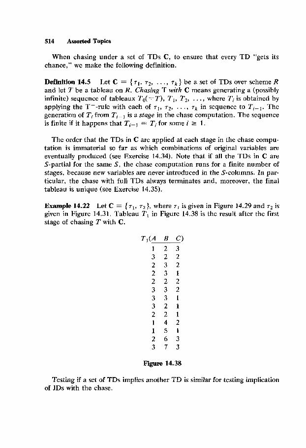
Example 14.22 Let C = ( TV, r2 >, where 71 is given in Figure 14.29 and r2 is given in Figure 14.31. Tableau T1 in Figure 14.38 is the result after the first stage of chasing T with C.

T,(A B ‘3 1 2 3 3 2 2 2 3 2 2 3 I 2 2 2 3 3 2 3 3 1 3 2 1 2 2 1 1 4 2 1 5 1 2 6 3 3 7 3

Figure 14.38

Testing if a set of TDs implies another TD is similar for testing implication of JDs with the chase.


Definition 14.6 Let To, T1, T2, . . . be the sequence of tableaux generated when chasing To with a set of TDs. The limit of this sequence is the tableaux

T”= T*U T, UT2 w a--.

Note that T* might be infinite.

Theorem 14.9 Let C be a set of TDs over scheme R and let T = (T, w ) be an S-partial TD on R. Let T* be the limit of the sequence To( =T), T1, T2, . . . generated in chasing T with C. C implies r on arbitrary relations if and only if T* contains a row w* such that w*(S) = w(S).

Proof We give only a sketch of the proof. For the “if” direction, assume that w * first appears after the kfh stage in the chase computation. That is, w * is in T, but not in TKel. Let Y be a relation in SAT(C) and let p be avaluation such that p(T) E 1. Following the chase computation leading up to Tk, we can show that T must contain a tuple t* such that p(w*)(S) = tYS). It follows that p(w)(S) = t*(S) and so Y satisfies 7. Notice that the theorem holds in this direction for finite relations instead of arbitrary relations.

For the “only if” direction, we first show that T*, as a relation, satisfies C. If T* does not contain a row w* that matches w on S, then T*, as a relation, is a counterexample to C implying 7. Thus, if C does imply 7, w* must exist.

Example 14.23 Let r be the A C-partial TD in Figure 14.39. Note that the hypothesis rows of 7 correspond to the tableau T in Figure 14.30. If C is the set of TDs in the last example, we see that C implies r. From that example, we know that chasing the hypothesis rows of r with C gives a row that is (a1 cl) in the A C-columns.

7(A B C)

al b2 ~3

a3 b2 ~2 a2 b3 ~2 a2 b3 ~1 a2 b2 ~2

a, bl cl

Figure 14.39

516 Assorted Topics

14.2.5 Generalized Functional Dependencies

In Section 9.3 we briefly examined the structure of projections of SAT{ F ) for a set of FDs P. Projecting SAT( { A -E, B -E, CE - D})ontothescheme A B C D we came up with the following “curious” dependency that any relation in the projection must satisfy: If tl, t2, and t3 are tuples in r(A B C D) such that

1. t,(A) = t3(A) 2. t,(C) = t,(C) 3. t2(B) = t3(B)

then

4. t,(D) = Q(D).

This constraint is an example of a generalized functional dependency, which can be written in a notation similar to that for TDs, as shown in Figure 14.40. The rows above the line are again called hypothesis rows. The equality below the line is called simply the conclusion. A relation Y satisfies this particular generalized functional dependency if any valuation p that maps the hypothesis rows into I necessarily has p(d,) = P(d3). We now give a formal definition.

Y(A B C D) WI al b2 CI dl ~2 a2 h cl 4 ~3 al bl ~2 d3

dI = d3

Figure 14.40

Definition 14.7 A generalized functional dependency (GFD) on a relation scheme R is a pair y = (T, a = b), where T is a set of rows on R, called hypothesis rows, and a and b are two variables from the rows in T. The equality a = b is called the conclusion. A relation r(R) satisfies the GFD y if for every valuation p of T such that p(T) C r, p(a) = p(b). The GFD y is trivial if it is satisfied by every relation on r; it is typed if no variable appears in more than one column of T and a and b come from the same column of T.


We shall assume that all GFDs are typed, henceforth. Figure 14.40 shows how GFDs are written. Not every FD is equivalent to a GFD, but only because GFDs enforce equality in only one column. Any FD with a single attribute on the right side can be expressed as a GFD, so any FD is equivalent to a set of GFDs.

Example 14.24 Consider the FD A B + C on scheme A B CD. Figure 14.41 shows the equivalent GFD for this FD.

-164 B C D) abc d a b cr d’

Figure 14.41

It is possible to give a complete set of inference axioms for GFDs, but we shall not do so, since such axioms essentially mimic the chase computation. Complete axiomatizations also exist for TDs and GFDs together, although they are for implication on arbitrary relations if partial TDs are allowed. We give one axiom for inferring TDs from FDs.

GTl Let X -+ A be a nontrivial FD over relation scheme R and let Y = R - (XA). This FD implies the TD 7 shown in Figure 14.42. Note that we use a little shorthand in 7. For instance, x1 and x2 stand for sequences of variables over X that are distinct in every column.

7(X A Y)

Wl Xl al YI ~2 XI a2 ~2

w3 x2 a2 ~3

Figure 14.42

Example 14.25 Figure 14.43 shows a TD 7 implied by the FD A B -+ C on scheme A B C D.

518 Assorted Topics

dA B C D)

~1 h cl dl a1 bl CL2 d2

a2 b2 ~2 4

Figure 14.43

To see that the TD r in GTl follows from the FD X + Y, consider the GFD y in Figure 14.44 that is equivalent to X + Y. Let r be an arbitrary relation on R. Let p be a valuation that maps wl-w3 into r. If r satisfies y, then p(al) = p(a2), since the fist two rows of y are the same as the first two rows of 7. It follows that p(w) is in T, since p(w) must equal p(wj).

-AX A Y)

Wl Xl a1 Yl “2 Xl a2 ~2

a1 = a2

Figure 14.44

Axiom GTl can be generalized from FDs to GFDs (see Exercise 14.39). The derived TD can be used in place of the FD when inferring TDs from a set C of FDs and TDs. That is, if we form C ’ by replacing every FD in C with the TD given by GTl, C and C ’ imply the same TDs (see Exercise 14.40).

Extending the chase computation to GFDs is fairly straightforward.

G-rule Let y = (Tl, a = b) be a GFD over scheme R. Let T2 be a tableau over R. For any valuation p such that p(T,) z T2 and p(a) # p(b), identify p(a) and p(b) in T2.

The chase computation under a set C of GFDs on a tableau T is just the application of the G-rule for GFDs in C until no more variables in T can be equated. The computation terminates, because no new rows or variables are introduced in T. Although not proved here, the result is unique given the proper mechanism for renaming variables when identifying them (such as always choosing the one with the lower subscript to replace the other). Since the result of the chase with GFDs is unique, we may denote it as chase&T).


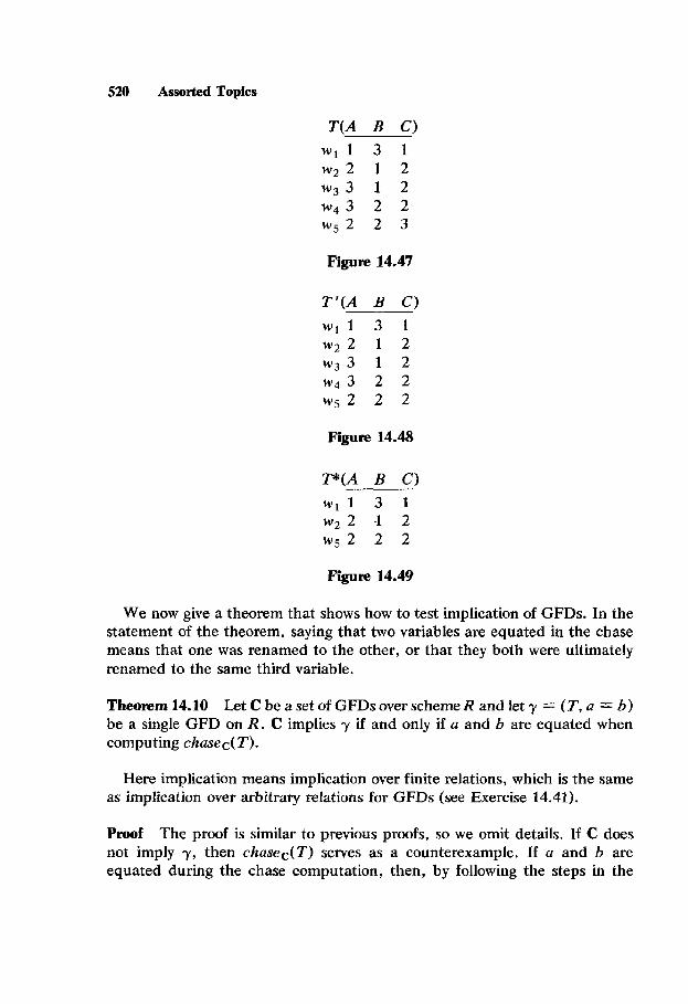
Example 14.26 Let C = { yl, y2 }, where y1 and y2 are as shown in Figures 14.45 and 14.46. Let T be the tableau in Figure 14.47. Again, we give only the subscripts for the variables in T for simplicity, so, for instance, “2” represents different variables in different columns. We first apply the G-rule for y1 to T. There is a valuation p1 from the hypothesis rows of y1 to T such that

dud = w3

l&2) = w4

Pb3) = w5

Thus, we identify p(c,) and p(cs), that is, 2 and 3 in the C-column. The result is tableau T’ in Figure 14.48. We adopt the rufe of replacing higher subscripts with lower ones. We next apply the G-rule for y2 to T’ using the valuation p2 where

P(Vl) = w2

P(V2) = w3

P(V3) = w4

We can equate 2 and 3 in the A-column to obtain the tableau P in Figure 14.49. At this point, no more variables can be identified with the G-rule, so chasec(T) = r”.

y,(A B C>

~1 ~1 bz cl ~2 ~1 bl ~2

u3 a2 bl C3

Ct = c3

Figure 14.45

Y@ B C)

VI al bl cl 3 a2 bl ~2 ~3 a3 b2 CI

Figure 14.46

520 Assorted Topics

T(A B C)

WI1 3 1 w22 1 2 ws3 1 2 w43 2 2 w52 2 3

Figure 14.47

T’(A B C)

WI1 3 1 w22 1 2 wg3 1 2 w43 2 2 wg2 2 2

Figure 14.48

IPk(A B C)

Wil 3 1 w2 2 -1 2 w52 2 2

Figure 14.49

We now give a theorem that shows how to test implication of GFDs. In the statement of the theorem, saying that two variables are equated in the chase means that one was renamed to the other, or that they both were ultimately renamed to the same third variable.

Theorem 14.10 Let C be a set of GFDs over scheme R and let y = (T, a = b) be a single GFD on R. C implies y if and only if a and b are equated when computing chasec( T).

Here implication means implication over finite relations, which is the same as implication over arbitrary relations for GFDs (see Exercise 14.41).

Proof The proof is similar to previous proofs, so we omit details. If C does not imply y, then chasec(T) serves as a counterexample, If a and b are equated during the chase computation, then, by following the steps in the


computation, we can show that any valuation ,o from T into a relation r in SAT(C) must have p(a) = p(b).

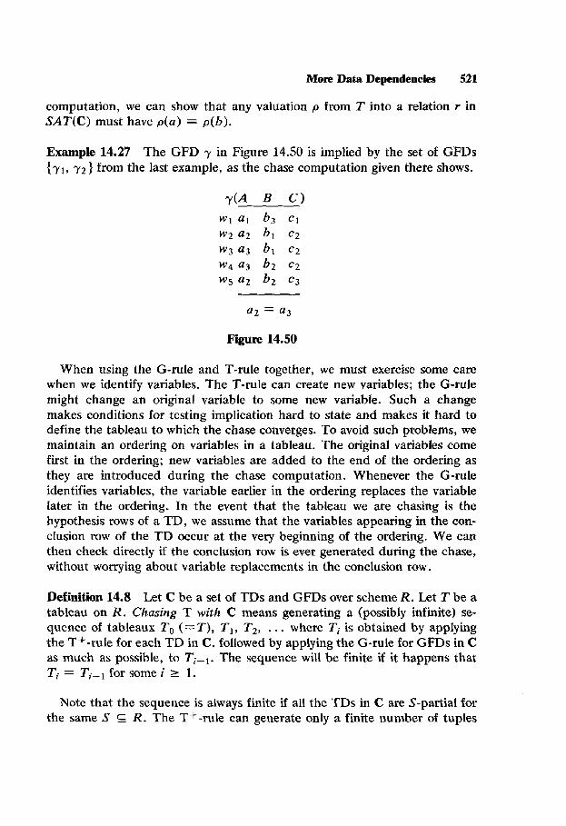
Example 14.27 The GFD y in Figure 14.50 is implied by the set of GFDs {r,, y2 } from the last example, as the chase computation given there shows.

$A B C) WI ai b3 ~1 ~472 a2 h ~2 ~3 a3 h ~2

~4 ~3 b2 ~2

~5 a2 b2 ~3

a2 = a3

Figure 14.50

When using the G-rule and T-rule together, we must exercise some care when we identify variables. The T-rule can create new variables; the G-rule might change an original variable to some new variable. Such a change makes conditions for testing implication hard to state and makes it hard to define the tableau to which the chase converges. To avoid such problems, we maintain an ordering on variables in a tableau. The original variables come first in the ordering; new variables are added to the end of the ordering as they are introduced during the chase computation. Whenever the G-rule identifies variables, the variable earlier in the ordering replaces the variable later in the ordering. In the event that the tableau we are chasing is the hypothesis rows of a TD, we assume that the variables appearing in the conclusion row of the TD occur at the very beginning of the ordering. We can then check directly if the conclusion row is ever generated during the chase, without worrying about variable replacements in the conclusion row.

Definition 14.8 Let C be a set of TDs and GFDs over scheme R. Let T be a tableau on R. Chasing T with C means generating a (possibly infinite) sequence of tableaux To (=T), T1, T2, . . . where Tj is obtained by applying the T+-rule for each TD in C, followed by applying the G-rule for GFDs in C as much as possible, to TimI. The sequence will be finite if it happens that Ti = T;-l for some i 1 1.

Note that the sequence is always finite if all the TDs in C are S-partial for the same S E R. The Tf-rule can generate only a finite number of tuples

522 Assorted Topics

with new combinations of variables in the S-columns. We cannot define the limit of the chase sequence as we did for TDs alone, since rows can be changed from one stage to the next. We need to identify the rows at a given stage that undergo no subsequent changes.

Definition 14.9 Let TO, T1, Tz, . . . be the sequence of tableaux generated by chasing a tableau T with a set C of TDs and GFDs. Relative to this sequence, a row w in Ti is stabilized if w appears in Tj forj 1 i. Let STABLE(Ti) denote all the stable rows in Ti. The limit of the sequence To, T1, T2, . . . is the tableau

T*: = STABLE(To) U STABLE( T1) U STABLE( Tz) - - - .

(P may be infinite.)

An important point is that P, as a relation, satisfies C. Note that if some set of rows wl, w2, . . . , wk in 13K gives rise to a violation of a GFD in C, then at least one of them is not stabilized, since it would have the offending value changed by the G-rule.

The next Theorem summarizes implication of TDs and GFDs for arbitrary relations.

Theorem 14.11 Let C be a set of TDs and GFDs over scheme R and let T be a tableau on R. Let P be the limit of the sequence To( = T), T1, T2, . . . generated when chasing T with C. We have

1. C implies the S-partial TD (T, w) if and only if Iph contains a row w* such that w*(S) = w(S), and

2. C implies the GFD (T, a = b) if and only if a and b are equated in generating P .


It follows from the theorem that TDs by themselves imply only trivial GFDs. Note that the tests for implication of FDs and IDS in Sections 8.6.3 and 8.6.4 are specializations of this theorem.

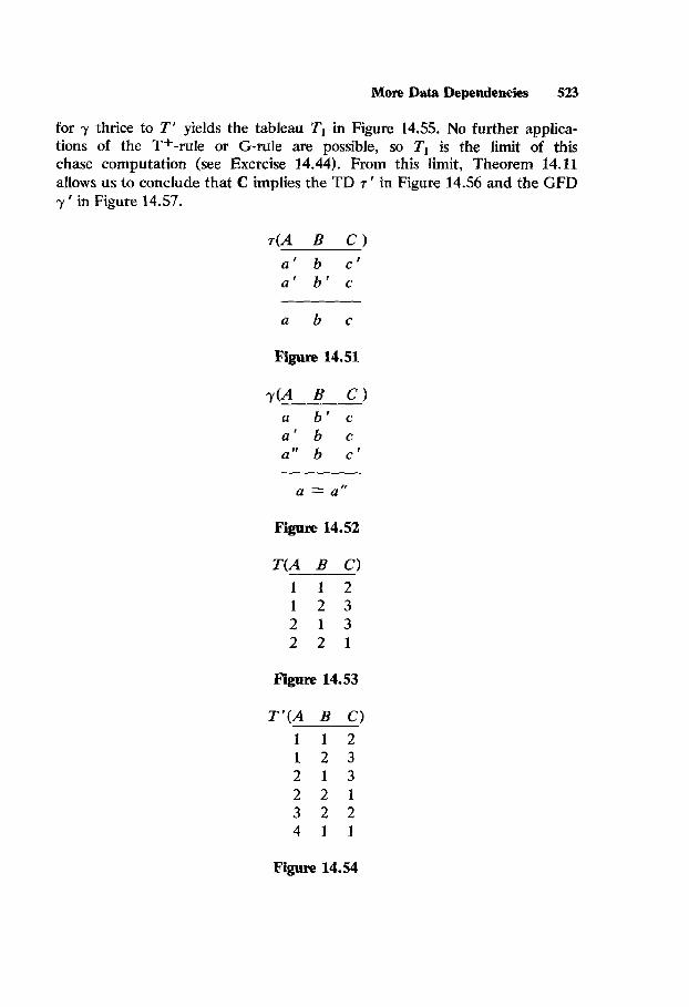
Example 14.28 Let C = { 7, y 1, where r is the TD in Figure 14.51 and y is the GFD in Figure 14.52. Let To be the tableau in Figure 14.53. Again, we show only subscripts for simplicity. Consider chasing To with C. Applying the T+-rule for r gives the tableau T’ in Figure 14.54. Applying the G-rule


for y thrice to T’ yields the tableau Tl in Figure 14.55. No further applica- tions of the T+-rule or G-rule are possible, so Tl is the limit of this chase computation (see Exercise 14.44). From this limit, Theorem 14.11 allows us to conclude that C implies the TD T’ in Figure 14.56 and the GFD y ’ in Figure 14.57.

a’ b c’ a’ b’ c

a b c

Figure 14.51

r(A B c) a b’ c a’ b c a” b c’

a = arr

Figure 14.52

T(A B C)

1 1 2 1 2 3 2 1 3 2 2 1

Figure 14.53

T’(A B C)

1 1 2 1 2 3 2 1 3 2 2 1 3 2 2 4 1 1

Figure 14.54

524 Assorted Topics

TIM B 0 1 1 2 1 2 3 1 1 3 1 2 1 1 2 2 I 1 1

Figure 14.55

T’(A B C)

a1 bl c2

al b2 ~3 a2 h ~3 a2 b2 ~1

Figure 14.56

r’(A B Cl al bl ~2 ~1 b2 ~3

a2 h ~3 ~2 bz ~1

a1 = a2

Figuw 14.57

14.2.6 Closure of Satisfaction Classes Under Projection

Recall the notation introduced in Chapter 8 for expressing the class of all relations on a given relation scheme R that satisfy a set of constraints C, SAT,(C). Also recall that we may extend a relational operator to sets of relations in an element-wise fashion. Thus, if P is a set of relations on scheme R, andX G R, then


In Chapter 9 we briefly considered the question of whether rrx(SATR(C)) necessarily can be expressed as SATx(C ‘) for C and C ’ coming from given classes of dependencies. The answer was “no” if C and C ’ are both FDs or both MVDs.

In this section we show that if C is TDs and GFDs, then there is always a set C’ of TDs and GFDs such that nx(SATR(C)) = SATx(C ‘). However, to make the equality hold, we must interpret SAT(C) as including both finite and infinite relations satisfying C. We shall see that if the TDs in C are restricted to be full, then SAT(C) may be interpreted as only the finite relations satisfying C.

For C a set of TDs and GFDs over R and X s R, ~~((2) will mean the set of TDs and GFDs over scheme X that are satisfied by all relations in n@AT(C)). Clearly, ?r&S’AT,(C)) s SATx(nx(C)), so if there is any set C ’ such that ‘I~,(SAT~(C)) = SAT-JC ‘), ~~(0 will also be such a set. It turns out that 7rx(C) can be infinite, with no equivalent finite set of TDs and GFDs (see Exercise 14.43, so there is no algorithm guaranteed to generate all of rx(C) in general. The next lemma, however, points out some of the dependencies in 7rx(C).

For a tableau T over scheme R and X E R, let T(X) be the tableau over scheme X obtained by restricting the rows in T to X.

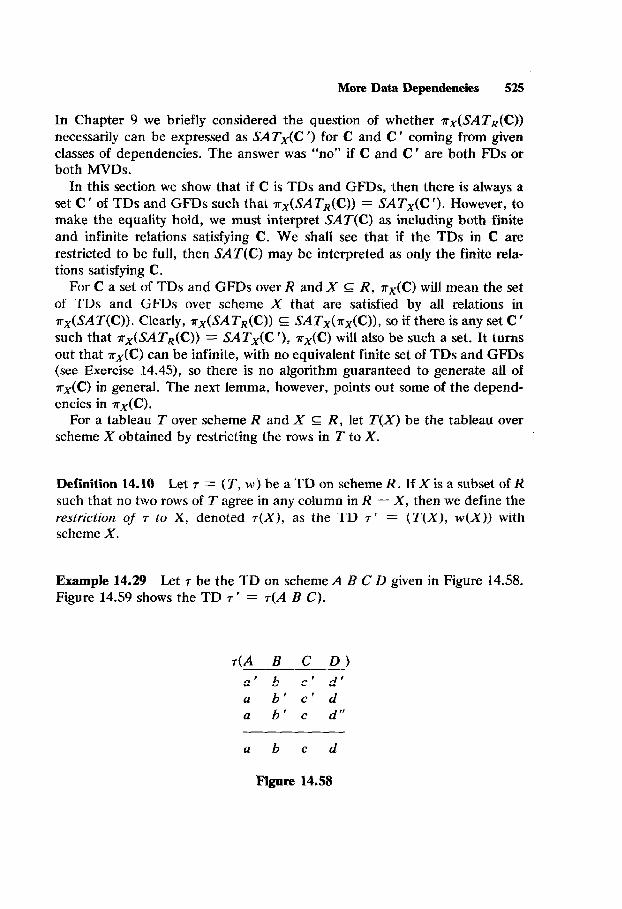
Definition 14.10 Let 7 = (T, w ) be a TD on scheme R. If X is a subset of R such that no two rows of T agree in any column in R - X, then we define the restriction of 7 to X, denoted 7(X), as the TD 7’ = (T(X), w(X)) with scheme X.

Example 14.29 Let 7 be the TD on scheme A B CD given in Figure 14.58. Figure 14.59 shows the TD 7’ = 7(A B C).

a’ b c’ d’ a b’ cr d a b’ c d”

a b c d

Figure 14.58

526 Assorted Topics

7’(A B C)

a’ b c’ a b’ c’ a b’ c

a b c

Figure 14.59

Lemma 14.8 Let r be a TD over scheme R such that r(X) is defied. If r is a relation in SAT(T), then 7r,&) is in SAT(7(X)).


Definition 14.11 Let y = (T, a = b) be a GFD on scheme R. If X is a subset of R such that no two rows of T agree in any column in R - X and a and b occur in some column of X, we define the restriction of y to X, denoted -r(X), as the GFD y ’ = (T(X), a = b),

Lemma 14.9 Let y be a GFD on R such that y(X) is defined. If r is a relation in SAT(y), then xx(r) is in SAT(y(X)).

Proof Assume y = ( T, a = b). Let p be a valuation from T(X) into xx(r). Since no two rows of T agree outside of X, p can be extended to a valuation p ’ from T into r. Moreover, p can be extended so that p(rv(X>) = p ‘(W)(X), for every row w of T (hence for every row w(X) of T(X)). Since r satisfies y, p ‘(a) = p ‘(b). Since a and b appear in T(X), p(a) = p(b), so Q(Y) satisfies r(X).

Theorem 14.12 Let C be a set of TDs and GFDs over scheme R. If X is a subset of R, then

dsAT,tCH = SATx(rx(C)).

Proof As we remarked previously, the right set contains the left set. To show the other inclusion, let s be a relation in SATx(rx(C)). We exhibit a relation r in SAT,(C) such that 7rx(r) = s. Form s’(R) by extending each tuple in s to R with new values in the (R - X)-columns. Let r be the limit of chasing s ’ with C. In extending the chase to relations, we do allow identification of values in this instance. However, we show shortly that no identifica-

Limitations of Relational Aigebra 527

tions are made in the X-columns of s ‘, Since r is obtained by chasing with C, r is in SAT(C). We show that TX(r) = s.

Let t be any tuple in s and let t ’ be the extended version oft in s ‘. Suppose at some stage in the chase computation, some value in the X-columns of t ’ is changed by application of the G-rule. Interpreting s ’ as a tableau, we see that C implies a GFD y that has s ’ as hypothesis rows and whose conclusion equates two values in the X-columns of s ‘. Since all the values in the (R - X)-columns of s ’ are distinct, we apply Lemma 14.9 to show that y(X) is in 7rx(C), But y(X) has s as its hypothesis rows, and equates two values ins. Therefore, s violates nx(C), a contradiction. We conclude that t ’ remains unchanged in the X-columns during the chase computation. If t ” is the tuple in r corresponding to t ‘, then t”(X) = t ‘(X) = t. We conclude that s c q&J.

Now let t” be any tuple in r. Again interpreting s ’ as a tableau, we see that C implies the TD 7 that has s ’ as hypothesis rows and t” as the conclusion row. By Lemma 14.8, rx(C) contains the TD 7(X), which has s as hypothesis rows and t”(X) as the conclusion row. Since s satisfies 7(X), s must contain t”(X). Hence, s 3 TX(r), and so s = TX(r).

Theorem 14.12 is true for SAT(C) interpreted as finite relations satisfying C if C contains only full TDs and GFDs. Looking back in the proof, the relation r generated by chasing s ’ with C will be finite if C meets this restriction. In particular, the “finite relation” version of the theorem is true for C consisting of FDs and JDs (although Q(C) may have dependencies that are not .TDs or FDs).

14.3 LIMITATIONS OF RELATIONAL ALGEBRA

We have used relational algebra as the “yardstick” for a complete query system. In this section we show that this definition for complete can be dis- puted, since there are some natural operators on relations that cannot be expressed by relational algebra. To be exact, we show that there is no algebraic expression E that specifies the transitive closure of a two-attribute relation.

Definition 14.12 Let r be a relation on a two-attribute relation scheme, call it A IAz, where dom(Al) = dom(A2). The transitive closure of r, denoted rf, is the smallest relation on A,Az such that r c r+ and r+ satisfies the untyped TD

528 Assorted Topics

441 A21

a b b c

a c

Note that this definition is symmetric in Al and AZ.

Example 14.30 If T is the relation in Figure 14.60, then Figure 14.61 shows r+ .

r(A B) 1 2 2 1 2 3

Figure 14.60

r+(A B)

1 2 2 1 2 3 1 1 1 3

Figure 14.61

In the next theorem, we shall construct something that looks like a domain calculus expression, except we shall use a different set of atoms than usual. Assume + is a relation on scheme AlA where dom(Al) = do. We use the atom #(a b) to mean that b is i “steps away” from a in I-. More precisely, for i 1 0, #(a b) is true when there are values al, a2, . . . , aiel in dom(Al) such that (uar), (a1 a~), {u2u3), . . ., {a+r b) are all tuplesinr. We let r”(a b) mean a = b and a appears in r. That is, r” is equality on values in r. Finally, for i < 0, r’(a b) if and only if r-‘(b a). Note that &(a b) and r’(b c) together imply r’+j(a c) and that rr(a b) if and only if (a b > E I*.

Example 14.31 For relation Y in Figure 14.60, rO(l l), r1(2 l), r2(1 l), and r2(1 3) are all true, while r0(4 4), r’(l I), and r2(1 2) are all false.

Limitations of Relational Algebra 529

Theorem 14.13 Let A1 and A2 be two attributes with the same domain. There is no relational algebra expression E involving a relation r(A1A2) such that E(r) = rf for all states of r.

Proof Assume that the domain of A r and A2 is the positive integers with only the comparators = and # . While we do not allow inequality comparisons in selections, we shall use the order of the integers in our arguments. It suf- fices to show that there is some state of T for which E(r) # rf . We restrict ourattentiontostatesoftheform{(12), (23), . . . . (p-1p))forp > 1. We denote this state of Y by [PI.

We begin by showing that for any relational algebra expression over T and for sufficiently large p, there is a domain calculus-like expression

Ep = {b,(BI) b2(Bz) --- b,(B,)lf(b~, b2, . . -, b,))

such that EQ]) = E,([pJ). The b’s in E, are assumed to range over {I, 2, . . ., p }. Formulaf is constructed of atoms of the form r’(at at), where ai is a constant or one of the b’s, 1 I i 5 2, and the connectives A, V and 1. A literal off is an atom or its negation and a clause off is a conjunction of literals. In the remainder of the proof, b’s and d’s are variables, c’s are constants and u’s are either.

The important property that Ep will have is that the form off will depend on E but not on p. The value of p will appear in f as a constant, but the number of literals and clauses in f is independent of p.

The proof that Ep exists is done by induction on the number of operators in E. By Theorem 3.1, we shall assume that E contains only the relation symbol Y, single-attribute single-tuple constant relations, selection with a single comparison, natural join, union, difference, renaming, and projection. We further assume that any projection removes exactly one attribute.

Basis If E has no operators, then E is r or (c : B > for some constant c. In the first case,

In the second case,

as long asp is sufficiently large that c appears in lp] (that is, p 1 c).

530 Assorted Topics

Induction We consider the form of E by cases. In all the cases, we assume that E’ and E” are subexpressions of E with corresponding calculus-like expressions

E; = {WV b,(B,) - -. b,W,,)If’(b,, b2, . . . , b,,)}

and

E; = {d,(D,) dz(DJ . . . d,(D,)(f”(dl, dz, . - . , d,)}.

1. Selection E = a&E ‘). Ep has the form

-ib,(Bd bzU-32) - - - b,(B,)lf’(b,, b2, . . . , b,) n g}

where g is r”(bj b,i), 1 r”(bi bj), r”(bi c) or 1 r”(bi c) depending on if the selection condition C is Bi = Bj, Bi # Bj, Bi = c, or Bi # c, respectively.

2. Join E = E ’ W E”. Assume that B1, B2, . . . , BR are the same as D 1, D2, . . . , Dk in Ed and Ei, Ep is then

ib,(B,) bzU%) - ’ - b,,,(B,,,) d/c+l(Dk+d . - - &(D,)I

f’tb,, b2, . . ., b,) WV,, b2, . . ., bk, dk+1, . . ., d,)).

3. Union E = E’ U E”. For E to be a legal expression, E; must have the form

Ibl(B1) bz(B2) * . . b,(B,)lf”(b,, b,, . . . , b,)}.

Ep is

(b#h)b2(&) - - - b,(&)Jf’(b,, 62, . - . , b,) v f”(bl, b . . ., b,)l.

4. Difference E = E ’ - E “. E,, ” must be as in Case 3. E,, is

{ bl(BJ bdBd .+. b,(B,)lf’(b,, b2, . . ., b,) A If’Yb,, bz, . . ., b,)).

5. Renaming E = aBiGD(E 7. Ep is

{b,(B,) b(B2) . . - hi(D) . a. b,(B,)lf’(bl, b2, . . . , b,)).

6. Projection E = rx(E’), whereX = BIB2 . . * B,-,. This is the hard case to handle. Assume m > 1 and that f ‘(bl, b2, . . . , b,) has the form

Limftations of Relational Algebra 531

fl(blt b2, . . ., b,) Vfi(bl, bz, . . ., b,) v - - - vfq(bl, bz, . . ., b,),

where each fi is a clause (f ’ is then said to be in disjunctive normalform or DNF). It is an elementary theorem of logic thatf ’ can be put into DNF if it does not already have that form. E,, could be represented as

{b,(h) b2tBd 1. e bra-,tKn-~)l~ W~,)f’tb~t bz, . . ., b,)),

but we do not want the existential quantifier. This expression is equivalent to

MJV &(Bz) . - e b,-ltB,-l)( (3 b,W,)fl(bl, b2, . . ,, b,)) v (3 b,(B,)f#l, b2, . . ., b,)) v . . . v (3 bnW,)f,th 62, . . . , b,))),

so we consider only the case wheref ’ is itself a single clause. Before we attempt to remove the existential quantifier, we do some

manipulations off ‘. For every atom that mentions b, , we move b, to the first slot, if it is not already there, using the identity #(a b,) = r-‘(b, a). We can leave out any literal of the form r”(b, b,) or 7 r’(b, b,), i # 0, as they are always true for [p]. Likewise, 1 r”(b, b,) or r’(b, b,), i f 0, can be replaced by 1 ro(bl b,), as they are always false for [p].

Two possibilities remain.

6.1 There is no literal of the form r’(b, a) in f ‘. That is, any atom mentioning b, is negated inf’. Letf (b,, b2, . . . , b,-l) be the conjunction of all the literals inf’ that do not mention b,. We claim that when p is sufficiently large, for any m - 1 constants cl, c2, . . . , cmV1 chosen from (1, 2, - * *, PI,

f(c1, c2, * * *, cm-,) = 3 b,f ‘(cl, ~2, . . ., cm-~, b,).

The right side implies the left side, since cl, c2, . . . , c,-, must satisfy every literal that does not mention b,. In the other direction, if p is sufficiently large, there is always some constant c, that makes every literal of the form lr”(b, c) inf(ci, c2, . . ., cmwl, b,) true when 6, is replaced with c,. Each such literal can prohibit only a single value for c,. Since the number of literals in f’ is fixed, but we allow p to be as large as necessary, there is always a choice for c,. Thus, if f(cl, c2, . . . , c,-~) is

.:

532 Assorted Topks

true, so is 3 bmf’(cl, c2, . . . , c,-~, b,), by the choice of c, for b,. In this case we have

6.2 The other possibility is that there is some literal of the form r’(b, a) inf’. In this case, to fonnf, we remove r’(b, a) and make a replacement for any other atom mentioning b,. Since we have the relative position of 6, and a, we can convert any reference to b, to a reference to u.

If the literaf that mentions 6, is i(b, a ‘), we replace it with i-‘(a u ‘). Certain simplifications can then be made. For example, any literal of the form rk(c c ‘) can be removed if c + k = c ‘, or replaced by 1 r”(bl bl) if c + k # c ‘. Similarly, any literal of the form rk(u 6) can also be replaced by lr”(bl b,) if )K] r p.

To finish formingf, we must add a few more literals if the a in r’(b, a) is actually bR for some 1 I k I m - 1. If i > 0, we must conjoin the literals l&( 1 bR), 0 5 I < i. Since 5, is at least i steps away from b, , it must be at least i steps away from 1. If i < 0, we conjoin 1 r[(bkp), 1 I 1 5 -i.

We leave Exercise 14.48 to show that

f@l, b2, . . ., b,--1) = S,,f’(b,, b2, . . ., b,).

The final expression, as in the last subcase, is

=P = -tbl(B,)b2(Bz) -a- b,-,(B,-dlf(b,, b2, . . ,, b,-,)).

We have completed the case for projection. We now know that if E is a relational algebra expression as in the hypothesis of the theorem, for a sufficiently large choice of p, there is an expression

such that E,([p]) = [p] +. We may assume thatf is in DNF. We now argue that EP cannot correctly compute [p]+. It is important that

the form off is the same regardless of the choice of p (as long as p is sufficiently large that we can form f correctly). In particular, the number of clauses in f is independent of p. The only place p enters the construction (other than as a constant in E) is in the literals 1 r’(b, p) that we add in subcase 6.2. Thus, we can convert E, toE, ‘, p ’ L p, by replacing each 1 r’(b,p) by 1 r’(b, p ‘). Another property off is that, by our simplifications, f con-

Computed Relations 533

tains no atom of the form #(a1 a~) for Ii] 2 p, nor any atom of the form rqc1 c2).

Suppose each clause off contains an unnegated literal #(al ~2) where ui, 1 5 i 5 2, is bl, bz, or a constant, but not both a, and a2 are constants. The number of clauses in f is independent of p. Say there are k of them, so we are dealing with k unnegated literals. If p is sufficiently larger than k, then there are choices cl and c2 for bl and b2 such that (cl c2) f [p]+, but replacing bl and bz by c1 and c2 makes each of the k unnegated literals false. For example, if iis the magnitude of the largest superscript of any of the unnegated literals, and C is the largest constant appearing in any of them, let c1 = T + C + 1 and let c2 = 2? -I- C + 2. By such a choice of cl and ~2, we have f(cl, c2) is false, so (cl c2> is not in E,([p]), but (cl ~2) is in [pl+, a contradiction.

If every clause off does not contain an unnegated literal, then there is some clause in which every literal has the form 1 v’(ul u2), where ui, I I i 5 2, is bl, b2 or a constant, but not both al and u2 are constants. Since there are a fixed number of literals in this clause, if p is large enough, we can choose values c t and c2 for bl and b2 such that ( c1 c2> is not in [p]+, but all the atoms in the clause are false. Since all the atoms are false, all the literals are true, so the clause is true andf(cl, c2> is true. (How do we pick cl and c2?) Hence, (cl ~2) C E,(Iplh a contradiction. We see that in any case, there is somep for which E,([p]) # [PI +. Since Ep is equivalent to E, E cannot compute transitive closures correctly for all states of r.

There have been several proposals for extending relational algebra so it can express more operations on relations. These proposals generally involve addition of programming language constructs or fixed-point operators. The query language QBE, which we cover in the next chapter, includes constructs specifically for dealing with transitive closures of relations (for relations whose closures are anti-symmetric).

14.4 COMPUTED RELATIONS

14.4.1 An Example

Consider a relation schedule(FLIGHT# FROM TO DEPARTS ARRIVES) containing flight information for our mythical airline. Suppose we want to create a relation length(FLIGHT# FLYTIME) that gives the duration of each flight. One approach is to use a database command to extract tuples

534 Assorted Topics

from the relation, perform a calculation in some general-purpose programming language, and use another database command to insert tuples into Length. That is, we embed calls to the database system within programs in some standard programming language. If the times in schedule are local, the program doing the duration calculation has to know what the time zone is for each city served. It would simplify the program if the database system could connect each city with its time zone. We can keep a relation inzone(CITY ZONE) giving the time zone for each city served. We can then define two virtual relations

and use them to define a third virtual relation

Zonetimes = =FZIGHT# DEPARTS Z-ONE ARRZVES ~odschedule w fromzone W tozone).

The program can then access zortetimes to compute length without having to look up time zones for cities.

Suppose we want length to be a virtual relation, so its state is always consistent with that of schedule. We need to do the computation of length en- tirely within the database system. We could have a relation lasts(DEPARTS FZONE ARRIVES TZONE PLYTIME) that gives the duration for all combinations of departure and arrival times and zones. If we had lasts, we could define length as

?~F~GHT# JFL y~~~,&zonetirnes W lasts).

While such an approach is conceivable, lasts will be a huge relation if it includes all possible combinations of times and zones. Even if we took this approach, we would probably need a program to calculate all the tuples in lasts.

What would be nice is if fasts only contained the tuples needed to correctly compute length. There is no way to know in advance what tuples will be needed in lasts, so it would be desirable to compute the proper tuples upon demand. That is, we would like to implicitly embed calls to programs within database commands. Rather than associating any stored extension with lasts, we instead associate a program that calculates PLYTIME, given values for DEPARTS, FZONE, ARRIVES, and TZONE, so tuples can be created upon demand when computing length.


We call a relation whose extension is a function a computed relation. To distinguish computed relations from relations with stored extensions, we call the latter tabular relations.

We cannot use the computed relation fasts in arbitrary expressions, for example

The procedure associated with lasts does not work in the right direction for use in computing dtimes. We can associate other programs with lasts to generate tuples when values on other sets of attributes are given. To handle dtimes, we would need a procedure that generates all DEPARTS FZONE TZONE-values for a given ARRIVES FLYTIME-value, While such a procedure is not unreasonable, we probably would not want to deal with a procedure that generates all DEPARTS FZONE FLYTIME-values for a given ARRIVES TZONE-value. In general, while we can associate several procedures with a computed relation to handle different sets of input attributes, it is unlikely that there will be a procedure for every set of attributes.

If we associate a procedure with lasts to compute an ARRIVES-value from a DEPARTS FZONE TZOME FLYTIME-value, we can evaluate the expression

TTO FROM ARIUd~DEPARTS=& t5a.FLYTIME=2:40(laStS w

fromzone W tozone))

to get the arrival times in various cities of a flight that departs at 8:14a and lasts 2 hours and 40 minutes. It may not be immediately apparent that we can evaluate this expression given the procedural extension of lasts, but we shall show shortly that it is possible.

The procedures associated with computed relations need not return a value for every possible value on the input attributes. For lasts, for any set of four attributes, there is a function that will return a value on a fifth attribute, so Iong as there is a legal value. However, there may not always be a legal value for the fifth attribute to go with a given value on the other four. For instance, if we have (9:20a Pacific 1:2Op 2:40) as a value on DEPARTS FZONE AR- RIVES FLYTIME, there is no value for TZONE that will form a legal tuple in lasts.

Sometimes we cannot evaluate a given expression involving a computed relation because certain procedures are absent from the relation’s extension.

536 Assorted Topics

In some of those cases, however, we may still be able to test if a particular tuple is in the relation represented by the expression. Suppose the only procedures associated with lasts are ones that generate a fifth value, given four others. Consider again the expression

While with the specified computed extension for lasts we cannot evaluate dtimes, we can test if a particular tuple, say (10:SOa Eastern), is in dtimes. We can make this test because it amounts to evaluating the expression

~DEPARTS=10:5On,FZONE=Eastem ( TDEPAR TS IZONE

(~~~~~=1:10p.FL~~~E=2:20(~aasts))),

for which the given procedural extension of lasts is adequate. The next section examines the problem of determining, given a restricted

algebraic expression involving computed relations, if the expression can be effectively evaluated, tested for membership, or neither.

X4.4.2 Testing Expressions Containiig Computed Relstions

We shall not worry much about the exact mechanism for specifying the procedures that make up the extension of a computed relation. We are mainly concerned with which sets of attributes can be used to determine values for other attributes.

To develop the theory of computed relations, it helps to imagine that any computed relation r(R) does have a tabular extension, although that extension might be infinite. We shall use simply r to denote that extension. For X, Y c R, we say there is a computed dependency (CD) of Y on X in T, written X =: Y, if given an X-value x, there is a procedure to compute ny(ux,,(r)). While not essential to the following discussion, it may clarify things to assume that a CD X =: Y implies the FD X + Y. That is, there is a function to compute a single Y-value given an X-value, so ?ry(ax,,(r)) contains at most one tuple. A determining set for r is any left side of a CD on r.

Example 14.32 If for the computed relation lasts in the previous section we could compute a fifth value from any four, lasts would satisfy the CDs


DPFZARTZ=:FT DPFZARFT=:TZ DPFZTZFT =: AR DPARTZFT =: FZ FZARTZFT =: DP,

using the abbreviations DP, FZ, AR, TZ and FT for DEPARTS, FZONE, ARRIVES, TZONE and FLYTIME. To recast remarks in the previous section, it is conceivable that lusts could satisfy the CD

ARFT =: DPFZTZ,

but it is unlikely that the extension of lasts would contain a procedure that would give rise to

ARTZ=:DPFZFT.

We now define the terms listable and decidable for algebraic expressions involving computed relations. We limit ourselves to expressions with single- tuple constant relations, project, select on equality, and natural join. Recall that these constraints define the class of restricted algebraic expressions, for which equivalent tagged tableau queries exist. We actually define listable and decidable for tagged tableau queries. Recall the notation associated with a tagged tableau query. For a tagged tableau query Q, a database d, and a valuation p of Q, p(Q) C d means that p maps every row w in Q to a tuple in the relation in d with scheme tag(w). We then have

Q(d) = {dwo)ldQ) E d),

where w. is the summary of Q. Since we imagine every computed relation to have an extension, even if we cannot effectively compute it, Q(d) makes sense even when d contains computed relations.

To make our definitions, we need the algorithm MARK given in Figure 14.62. MARK marks symbols in a tableau query, succeeding if it marks all the symbols in the summary, and marks all matched symbols and a determining set for each row that is tagged with a computed relation. We assume MARK has global access to two set variables, TABULAR and COMPUTED, that give the sets of tabular and computed relations in the database.

538 Assorted Topics

Input: A tagged tableau query Q, and an array CDEP of sets of computed dependencies for each relation in COMPUTED. Output: true if all symbols of Q get marked; false otherwise. MARK( Q, CDEP) begin

1. Initialization. Mark all constant symbols in Q; for each row w E Q do

if tug(w) E TABULAR then mark every symbol in w;

2. Computation. 2.1. Propagate Marks.

while changes occur do for each marked variable a in Q do

mark all copies of a in Q, including those in the summary; 2.2. Apply CDs.

for each row w E Q do if tag(w) E COMPUTED then begin

for each CD X = : Y in CDEP( tug(w)) do If all the symbols in the X-columns of w are marked then mark all the symbols in the Y-columns of w

end;

3. Return Results If all the symbols in the summary are marked aud

every row tagged with a computed relation is marked on all its matched variables and on some determining set

then return (true ) eke retum( false)

end.

Figure 14.62

Example 14.33 Consider the tagged tableau query Qi in Figure 14.63, which corresponds to one of the expressions of the last section (where FR ab- breviates FROM). Assume the first five CDs from the last example hold on lasts and that relationsfromzone and tozone are tabular. Figure 16.64 shows


Q, after the initialization step in MARK. We use the symbol X for marks. Figure 14.65 shows Q1 after propagation of marks. Applying the CD DR FZ TZ FT =: AR, we may mark as in the first row, as shown in Figure 14.66. Finally, in the second pass through the computation step, the mark on us is propagated to the summary, so MARK returns true.

Q1(FR TO DR FZ AR TZ Fl- )

al a2 a5 8:14a bl as b2 2:41 (lusts)

al bl (fromzone)

a2 bz (tozone)

Figure 14.63

Q,(FR TO DR FZ ARTZ FT )

ai a2 a5 8:14a X b, as bz 2:41 X (lasts)

a1 x 61 x (fromzone)

42 x b2 X (tozone )

Figure 14,64

Q,(FR TO DR FZ ARTZ FT )

al X a2 X 45 8:14a X bI X a5 b2 X 2:41 X (lusts)

al X 61 X ( fromzone ) a2 X b2 X (tozone )

Figure 14.65

Q,(FR TO DR FZ AR TZ FT 1

alX azX a5 8:14a X br X as X b2 X 2:41 X (lasts )

al X bt X ( fromzone )

a2 X bz X (tozone)

Figure 14.66

540 Assorted Topics

Example 14.34 The tagged tableau query Q2, in Figure 14.67, also corresponds to an expression given in the last section. Assume again that lasts has the first five CDs in Example 14.32. If we apply MARK to Qz, the two constants in the first row get marked, but no other marks are made. Thus, MARK returns false for Q2.

Qz(DR F-Z AR TZ FT )

al a2

al a2 1:lOp bI 2:20 (fasts)

Figure 14.67

Definition 14.13 A tagged tableau query Q is listable relative to a set of CDs CDEP if MARK(Q, CDEP) = true.

Example 14.35 The query Q1 given in Example 14.33 is listable, while the query Qz in Example 14.34 is not.

We have done things in a rather backwards manner. Usually we define a property, and then give an algorithm to test for it. Here we have given the algorithm, and defined the property from it. We shall now show that the term “listable” is well-chosen-that for a listable query Q and a database d, we can indeed compute Q(d ). We leave it to the reader to show that there is no way, in general, to evaluate Q(d) if Q is not listable (see Exercise 14.51). To simplify the argument, we assume that each CD X = : Y implies the cot- responding FD X --f Y. Hence, for any relation r with CD X =: Y, we may assume a functionf xy that returns a Y-value for any X-value, or possibly a special value K (for kill) that indicates I contains no tuple with the given X-value. The argument can be generalized to allow several Y-values for a given X-value (see Exercise 14.53).

To evaluate a tagged tableau query Q on a database d, we need to find every valuation p of Q such that p(Q) s d. Let Qtab be the set of rows in Q whose tags are tabular relations and let Q,,, be the rows with tags that are computed relations. The possibilities for p are limited by its value on rows in Q tab. It is a straightforward enumeration to find every valuation p of Qtab such that p(w) E tag(w) for every row w in Qtab, that is, p(Qtab) c d. We assume that we start with such a valuation p for Qiab, and attempt to extend it to a valuation for all of Q. We know that p(c) must equal c for every constant c, so we can extend p to all the constants in Q. At this point p is defined on the symbols that are marked after the initialization stage of running


MARK on Q. The strategy of this argument is to show that we can extend p to any symbol marked during that computation.

Any symbol a that is marked during the propagation step must already have p(a) defined. If we apply a CD X =: Y on a row w to mark the symbols in the Y-columns, the X-columns must already be marked. Hence, we know the value of p(w(X)). Using the function fxu corresponding to the CD, we can get a Y-value y = f&~(w(X))). If y is actually K, we know there is no way to extend p so that p(w) E tag(w). Also, no extension is possible if p is already defined on w(A), A E Y, and p(w (A )) # y(A). If neither of these cases arises, then we may extend p to w(Y) by letting p(w (Y)) = y.

If we continue on in this manner, we either find at some point p cannot be extended, or it is extended to all the symbols that get marked by MARK. The valuation p might not be defined on every symbol in some row w E Q,,,. Let tag(w) = r(R). Even if p is not defined on all of w, since MARK succeeds on Q, for some determining set X of r, p is defined. Thus, if p is defined on exactly w(Z), for some 2 E R, we can determine if there is a tuple t in Y such that p(w(Z)) = t(Z). Since any variable in w(R - Z) is not marked, it cannot be matched, or Q would not be listable. Theoretically, then, p could be extended to all of w by letting p(w) = t. We may not actually be able to determine the value of t on attributes in R - Z, but it is sufficient to know that appropriate values exist. Since the summary, say WO, of Q gets marked, p(wO) is defined, and is a tuple in Q(d).

We have argued that any valuation’ p found by the method above can be extended to all of Q in such a manner that p(Q) c d. Starting with some valuation p such that p(Q) C d, it is not hard to see that if we restrict p to Qtab and then extend it by the method above, we end up with a valuation that agrees with p on all the marked symbols of Q, and hence has the same value on the summary. Therefore, we can find every tuple in Q(d).

We now turn to the definition of decidable. Let MARK’ be the algorithm MARK of Figure 14.62 modified so that all the symbols in the summary of Q are marked during the initialization step.

Definition 14.14 A tagged tableau query Q is decidable relative to a set of CDs CDEP if MARK ’ (Q, CDEP) = true.

Example 14.36 Referring back to Example 14.34, let Q2 be the tagged tableau query in Figure 14.67. Running MARK’ on Q2, we mark all the symbols in the summary and the constants during initialization, as shown in Figure 14.68. Propagating the marks on al and a2, and applying the CD

542 Assorted Topics

DR FZ AR FT =: TZ results in all the symbols of Q2 being marked. Hence MARK ’ returns true for Q2 and so Q2 is decidable.

Q2(DR FZ AR TZFT )

a1 x a2 X

a1 x a2 X 1:lOp X b, 2:20 X (lasts)

Figure 14.68

We now argue that for a decidable tagged tableau query Q and a tuple t, we can effectively decide if t E Q(d). Let R be the scheme of Q(d), and assume t is a tuple on R. Deciding if t E Q(d) is the same as determining if oR,,(Q(d)) has any tuples. Let wg be the summary of Q. We can form a query Q ’ for uR,,(Q(d)) by replacing any variable ai in the A,column of w. by the constant t(Ai). If w(&) is already a constant and not equal to t(A,), we can stop, for we know t is not in Q(d). Q’ is just Q with summary variables replaced by constants, so MARK succeeds on Q’ exactly when MARK ’ succeeds on Q. Therefore, if Q is decidable, Q ’ is listable, and we can effectively decide if t E Q(d) by computing Q’(d).

The definitions of listable and decidable implicitly assume that domains are infinite. If a domain is finite, we can enumerate its values as part of an evaluation strategy. For example, if we had a computed relation r(A B) with CD A =: B, and dam(A) is finite, we could compute the extension of r by enumerating the domain of A. Exercise 14.55 shows how to incorporate information on finite domains into the definitions of listable and decidable.

14.5 EXERCISES

14.1 Show that all the inference rules for FDs are valid rules of inference for logic when FDs are interpreted as propositional formulas.

14.2” Choose any complete set of inference rules for FDs. Show that these rules, when interpreted as inference rules in propositional logic, are a complete set of inference rules for the subtheory of propositional logic consisting only of formulas of the form X 3 Y.

14.3 Complete the proof of Lemma 14.1. 14.4 Show that all the inference rules for MVDs alone and MVDs with

FDs are valid rules of inference for logic when FDs and MVDs are interpreted as propositional formulas.

14.5 Prove Lemma 14.3. 14.6 Prove Lemma 14.5.

Exercises 543

14.7 Prove Theorem 14.2. 14.8 Let F be a set of FDs, each with a single attribute on the right side.

Define

MF= (X- Y[X-+A EF).

MF is F converted to MVDs. Use Theorem 14.2 to prove the following theorem of Beeri.

Theorem 14.14 Let F be a set of FDs and let M be a set of MVDs. ForanMVDX-++Y,FUMimpliesX++YifandonlyifMFUM implies X + Y.

14.9

One consequence of this theorem is that any procedure for implication of MVDs by MVDs can easily be converted to a procedure for the inference of MVDs by FDs and MVDs. Show that inference in the world of two-tuple relations is not the same as inference over regular relations for JDs and embedded MVDs.

14.10” Show that the correspondence of FDs and MVDs with formulas in propositional logic can not be extended to embedded MVDs in such a way as to preserve equivalence of implication.

14.11 Let Jbe a set of JDs over scheme R. Let X be a subset of R. Show that rx(SAT(J)) cannot necessarily be expressed as SAT(J’) for a set J’ of IDS over X.

14.12 Give the smallest relation containing the relation r below that satisfies the TD r in Figure 14.5.

r(A B C)

1 3 5 1 3 6 1 3 7 2 3 5 2 4 5 1 4 6

14.13 Give the smallest relation containing relation r above that satisfies the TD r in Figure 14.7.

14.14 Show that the TD r in Figure 14.5 is not equivalent to any JD. 14.15 Prove that any JD, full or properly embedded, is equivalent to some

TD.

544 Assorted Topics

Definition 14.15 A (typed) TD is simple if each column has at most one repeated variable.

14.16

14.17*

14.18”

14.19*

14.20

14.21

14.22

14.23

14.24

14.25 14.26

14.27 14.28*

14.29” 14.30

14.31

(a) Prove that if a TD is simple and full, then it is equivalent to some ID. (b) Give a simple TD that is not equivalent to any full or embedded JD. Show that any set of full TDs over the same scheme is equivalent to a single TD. Give a set of partial TDs over the same scheme that is not equivalent to a single TD. Prove that there are only three distinct TDs over a relation scheme with two attributes. (They are the trivial TD, the Cartesian product TD, and the TD in Figure 14.10.) Show that a TD can be expressed as a quantified predicate calculus formula with a single predicate symbol (for the relation). Note that if the TD is full, the formula uses no existential quantifiers. Prove that any relation that is a column-wise Cartesian product satisfies every TD over its scheme. (a) Consider the set of all S-partial TDs over a scheme R, where

S C R and S has two or more attributes. Show that there is a strongest TD and a weakest nontrivial TD in this set.

(b) Prove that there is no weakest nontrivial TD over any scheme of three or more attributes.

Prove that a full TD is trivial if and only if the conclusion row is also a hypothesis row. Characterize those TDs that are equivalent to JDs in terms of the graphs of the TDs. Give two different graphs for the TD 7 in Figure 14.13. Is every TD whose graph can be drawn as a triangle equivalent to an EMVD? Prove Theorem 14.6. Exhibit a chain of progressively stronger TDs, along the lines of Theorem 14.7. Hint: Consider cutting the graph G in Figure 14.20 at node i, and then overlaying nodes 1 and i. Finish the proof of Theorem 14.8. Let C be a set of S-partial TDs on scheme R and let r be an arbitrary TD on R. Show that if there is an infinite relation that satisfies C but violates T, then there is a finite relation with the same property. Show that the following inference axioms for TDs are correct. Let T = (T, w) be a TD. (a) Renaming If 7’ is formed from 7 by a one-to-one renaming of

symbols, then 7 implies T ‘. (b) Identification of variables If T’ is formed by replacing all oc-

Exercises 545

currences of some variable in T of 7 with a variable from the same column of T, then T implies 7 ‘. (Note that this axiom does not allow identifying a variable that only appears in w with a variable in T. )

(c) TransitiviQ Let 71 = (T1, w,) and 72 = ( T2, w2) where T1 2 T2 U { w2 }. TDs 71 and 72 together imply 73 = (T1 - ( w2), w,).

(d) Reflexivity The TD ({w 1, w) holds for any row w. 14.321’ Prove that Augmentation (Lemma 14.7), Weakening (Section

14.3.4), Renaming, Identification of variables, Transitivity, and Reflexivity (from the last exercise) are a complete set of inference axioms for implication of TDs on arbitrary relations.

14.33” Show that if the T-rule is restricted to generate only rows that contain

14.34

14.35

14.36

14.37

new combinations of original variables in a tableau, then some combinations of original symbols will not be obtained that would be obtained without the restriction. That is, provide an example tableau and some TDs where the T-rule cannot generate any new combination of original variables immediately, but will do so eventually. Let C be a set of TDs over scheme R and let T be a tableau on R. Show that chasing T with C produces the same combinations of original variables no matter what the order in which the TDs in C are used. Let C be a set of full TDs over a scheme R and let T be a tableau on R. Show that chasing T with C always gives a unique result for the tableau at the last stage. Referring to Example 14.23, show that neither TD in C by itself implies r. Which of the following relations satisfies the GFD y in Figure 14.40?

rl(A B C D)

1 3 5 7 1 4 6 8 2 3 6 7

r2(A B C D)

1 2 3 5 1 2 4 6

q(A B C D)

1 2 4 5 1 3 4 6

546

14.38 14.39

14.40

14.41

14.42

14.43

14.44

Assorted Topics

Give a syntactic characterization for when a GFD is trivial. Find an inference axiom along the lines of GTl that gives a nontrivial TD implied by a nontrivial GFD. Show that axiom GTl can be used to replace FDs with TDs when considering the TDs implied by a set of FDs and GFDs. Prove that implication of GFDs is the same for finite and arbitrary relations. Note that row w1 can be removed from the GFD y in Figure 14.50 to get an equivalent GFD. State and prove a general result about super- fluous rows in TDs and GFDs. Sketch the proof of Theorem 14.11. Be sure to indicate why our method for renaming variables when applying the G-rule is adequate. In doing a chase computation with TDs and GFDs, show that if the sequence of tableaux generated is finite, then the last tableau in the sequence is the limit of the sequence.

14.45” Let C be a finite set of TDs and GFDs. Demonstrate that xx(C) can have an infinite number of dependencies, and also not be equivalent to any finite set of dependencies. What if C happens to contain only FDs and JDs?

14.46 (a) Prove that there is a set of GFDs equivalent to xx(C) when C contains only FDs.

(b) Prove that there is a set of TDs equivalent to nx(C) when C contains only IDS.

14.47 Prove Lemma 14.8. 14.48 In Case 6.2 of the proof of Theorem 14.13, show that

f(b1, bf, . . ., b,-,) = 36, f’(b,, b2, . . . , b,).

14.49 (a) Let lasts and zonetimes be as defined in Section 14.4.1. Assume connects (F#l F#2) is a relation giving all pairs of connecting flights. Give an algebraic expression that defines a relation giving total duration and layover time for each pair of connecting flights.

(b) What CDs must lasts satisfy in order to be able to evaluate your answer to part (a)?

14.50 Let rl (A B C) and v2(C D) be tabular relations. Let s 1 (B D E) be a computed relation with CDs B = : D E and D E = : B. Let s2( C E I) be a computed relation with CD C E = : I. Convert each of the following restricted algebraic expressions to a tagged tableau query, and say which of the resulting queries are listable.

Bibliography and Comments 547

(8) ~,&&1 w 12 Da s2) (W SI w ~2 (0 dsl b-4 ~2)

(i) ~DI(S, Da s2)

14.51 Show that in general there is no effective method to evaluate a query that is not listable. Assume that all domains are infinite.

14.52” Does tableau query equivalence preserve listability? 14.53 Give a method to evaluate a listable query without the assumption

that a CD X =: Y implies the FD X -+ Y. 14.54 Which of the tableau queries you produced in Exercise 14.50 are

decidable? 14.55 Show how information on finite domains can be brought into the

theory of computed relations by using a single-attribute tabular relation r(A ) for every attribute A with a finite domain. The extension of r will be dom (A ).

14.6 BIBLIOGRAPHY AND COMMENTS

The connection between FDs and propositional formulas was first exhibited by DeIobel and Casey [1973], and was fully developed by Fagin [1977b]. Sagiv [1980] showed the connection between MVDs and formulas. The material in this chapter on the connection between FDs and MVDs together and propositional formulas, particularly the material on two-tuple relations and the proof of Lemma 14.6, is from Sagiv, Delobel, Parker, and Fagin [1981]. Namibar [1979] also points out the connection between MVDs and logical formulas.

Template dependencies were introduced by Sadri and Ullman [1980a], although they deal only with the typed case. They give a complete axiomatization for TDs and also show how to extend the chase to TDs. Sadri and Ullman [1980b] also show how to include FDs with the TDs in the chase. The material on examples and counterexamples for TDs, graphical representations, and implication on finite versus infinite relations is from Fagin, Maier, Ullman, and Yannakakis [1981]. GFDs were defined by Sadri [1980a, 1980b, 198Oc], who gives inference rules for TDs and GFDs together, ex-

548 Assorted Topics

tends the chase to GFDs, shows satisfaction classes are closed under projection, and defines a normal form with respect to TDs and GFDs.

There have been numerous dependency classes defined in attempts to over- come problems with existing classes or to produce a more expressive language of relational constraints. Nicolas [1978a, 1978b] introduced mutual dependencies, which are a kind of join dependency, and showed that FDs, MVDs and mutual dependencies can all be expressed in first-order logic. Maier and Mendelzon [1979] generalized mutual dependencies. Tanaka, Kambayashi, and Yajima [1979b] explore the properties of EMVDs. Parker and Parsaye-Ghomi [1980], and Sagiv and Walecka [1979] proved that there is no finite complete axiomatization of the EMVDs by themselves. Both proofs work by showing that for any k there is an inference axiom that says a certain k EMVDs imply some other EMVD T, but any k - 1 of those EMVDs only imply other EMVDs that are implied by the EMVDs singly. Thus, that inference axiom cannot be derived from any set of inference axioms with k - 1 or less hypothesis EMVDs. The latter pair of authors define the class of subset dependencies, which properly include the EMVDs, and which has a finite complete axiomatization. A subset dependency is a statement of the form

Sciore [1982], attempting to axiomatize JDs, had to generalize that class of dependencies slightly in order to do so, and conjectures there is no finite axiomatization of JDs. His dependencies were essentially TDs with the restriction that any column may contain at most two repeated variables.

Several people independently came up with classes of dependencies similar to TDs and GFDs. Fagin [198Oa] used Horn clauses to define embedded im- plicational dependencies (EIDs), which are equivalent to untyped TDs and GFDs (where we consider any typed dependency to also be an untyped dependency). Among other results, he shows that any set C of EIDs has an Armstrong relation, that is, a relation that satisfies exactly the EIDs in C. Fagin also shows closure of satisfaction classes of EIDs under projection. Yannakakis and Papadimitriou [1980] give the class of algebraic dependencies, which are set inequalities on algebraic expressions formed with projection and equijoin. They show that algebraic dependencies are equivalent to EIDs. Grant and Jacobs [1980] use logic to define a class of dependencies that are equivalent to “full” EIDs. That is, their class is equivalent to untyped full TDs and untyped GFDs. Paredaens and Janssens [1981] define generalized dependencies, which are equivalent to TDs and GFDs.

Beeri and Vardi [1980a, 1980b, 1980~1 define tuple generating dependen-

Bibliography and Comments 549

ties and equality generating dependencies, which correspond to untyped TDs and untyped GFDs, respectively. They prove a number of complexity and decidability results, such as finite and infinite implication are undecidable for EIDs and implication of S-partial TDs is decidable. They also show the inequivalence of finite and infinite implication for untyped dependencies. Chandra, Harel, and Makowsky [1981] show undecidability of infinite implication for typed EIDs and untyped TDs. They also show that implication of “full” EIDs is decidable, but exponential-time complete. There are recent reports from several researchers that implication for typed TDs is undecidable, but the decidability of EMVDs has yet to be resolved.

Hull 119811 explores the properties of EIDs, and proves that satisfaction classes of EIDs are closed under join.

Several types of dependencies of a flavor different from TDs and GFDs have been proposed. Lipski and Marek [1979] discuss constraints involving cardinalities. Ginsburg and Hull [ 19811 consider constraints involving ordered domains. Casanova [I9811 presents a class of dependencies called subset dependencies, but they are not the same as the subset dependencies of Sagiv and Walecka. Rather, they are inter-relational constraints that connect projections of two relations.

The proof that transitive closure is not expressible in relational algebra is due to Aho and Ullman 119791, and they give some proposals for extensions of the algebra. Banchilon [1978], Paredaens 119781, Chandra [1981], and Chandra and Hare1 [1980a, 198Ob] have all proposed other notions of query language completeness. The language specification for QBE (Query-by- Example) given by Zloof 119761 includes specific constructs for dealing with transitive closures.

The section on computed relations is adapted from Maier and Warren [1981a]. The ISBL query language, presented by Hall, Hitchcock, and Todd [1975] and Todd [1975, 19761, allows some forms of computed relations.

Exercises 14.2, 14.8, and 14.10 are from Sagiv, Delobel, Parker, and Fagin [1981]. The original proof of Theorem 14.14 is by Beeri [1980]. Exer- cises 14.17, 14.18, 14.19, 14.28, and 14.29 are from Fagin, Maier, Ullman, and Yannakakis [1981]. Answers to Exercises 14.32 and 14.33 can be found in Sadri and Ullman [1980a]. Exercise 14.39 is from Beeri and Vardi [1980a]. Exercise 14.45 on finite specification is taken from Hull [1981]. Ex- ercise 14.46 is from Sadri [1980a].

Documents

Maier, Chapter 14: Assorted Topics