Embed Size (px)
Citation preview
Chapter 2
MATHEMATICAL PRELIMINARIES
2.1 Introduction
The early forms of finite element analysis were based on physical intuition withlittle recourse to higher mathematics. As the range of applications expanded, for exampleto the theory of plates and shells, some physical approaches failed and some succeeded.The use of higher mathematics such as variational calculus explained why the successfulmethods worked. At the same time the mathematicians were attracted by this new fieldof study. In the last few years the mathematical theory of finite element analysis hasgrown quite large. Since the state of the art now depends heavily on error estimators anderror indicators it is necessary for an engineer to be aware of some basic mathematicaltopics of finite element analysis. We will consider load vectors and solution vectors, andresiduals of various weak forms. All of these require us to define some method tomeasure these entities. For the above linear vectors with discrete coefficients,VT = [ V1 V2
...Vn ], we might want to use a measure like the root mean square,RMS:
RMS2 =1
n
n
i=1Σ V2
i =1
nVT V
which we will come to call a norm of the linear vector space. Other quantities vary withspatial position and appear in integrals over the solution domain and/or its boundaries.We will introduce various other norms to "measure" these integral quantities.
The finite element method always involves integrals so it is useful to review someintegral identities such as Gauss’ Theorem (Divergence Theorem) :
Ω∫ ∇ . u dΩ =
Γ∫ u . n dΓ =
Γ∫
∂u
∂ndΓ
which is expressed in Cartesian tensor form as
Ω∫ ui ,i d Ω =
Γ∫ ui ni dΓ
where there is an implied summation over subscripts that occurs an even number of timesand a comma denotes partial differentiation with respect to the directions that follow it.That is, ( ),i = ∂( ) / ∂xi . The above theorem can be generalized to a tensor with any
4.3 Draft− 5/27/04 © 2004 J.E. Akin 26
Finite Elements, Preliminaries 27
number of subscripts :
Ω∫ Aijk ...q,r dΩ =
Γ∫ Aijk ...q nr dΓ .
We will often have need for one of the Green’s Theorems :
Ω∫ (∇ A . ∇ B + A∇2B) dΩ =
Γ∫ A
∂B
∂ndΓ
and
Γ∫ (A∇2B − B∇2A) dΩ =
Γ∫ (A∇B − B∇A) . n dΓ
which in Cartesian tensor form are
Ω∫ (A,i B,i + AB,ii ) dΩ =
Γ∫ AB,i ni dΓ
and
Ω∫ (AB,ii − BA,ii ) dΩ =
Γ∫ (AB,i − BA,i ) ni dΓ .
We need these relations to derive the Galerkin weak form statements and to manipulatethe associated error estimators. Usually, we are interested in removing the highestderivative term in an integral and use the second from last equation in the form
(2.1)Ω∫ AB,ii dΩ =
Γ∫ AB,i ni dΓ −
Ω∫ A,i B,i dΩ .
In one-dimensional applications this process is called integration by parts:
b
a∫ p dq = pq
b
a
−b
a∫ q dp.
Error estimator proofs utilize inequalities like the Schwarz inequality
(2.2)|a . b| ≤ |a| |b|
and the triangle inequality(2.3)|a + b| ≤ |a| + |b| .
Finite element error estimates often use the Minkowski inequality
(2.4)
n
i=1Σ |xi ± yi |
p
1/p
≤
n
i=1Σ |xi |
p
1/p
+
n
i=1Σ |yi |
p
1/p
, 1 < p < ∞ ,
and the corresponding integral inequality
(2.5)Ω∫ |x ± y|p dΩ
1/p
≤Ω∫ |x|p dΩ
1/p
+Ω∫ |y|p dΩ
1/p
, 1 < p < ∞ .
We begin the preliminary concepts by introducing linear spaces. These are a collection ofobjects for which the operations of addition and scalar multiplication are defined in asimple and logical fashion.
4.3 Draft− 5/27/04 © 2004 J.E. Akin. All rights reserved.
28 J. E. Akin
2.2 Linear Spaces and Norms
The increased practical importance of error estimates and adaptive methods makesthe use offunctional analysisa necessary tool in finite element analysis. Today’s studentshould consider taking a course in functional analysis, or studying texts such as those ofLiusternik [15], Nowinski [18], or Oden [20]. This chapter will only cover certain basictopics. Other related advanced works, such as that of Hughes [14], should also beconsulted. We are usually seeking to approximate a more complicated solution by a finiteelement solution. To dev elop a feel for the "closeness" or "distance between" thesesolutions, we need to have some basic mathematical tools. Since the approximation andthe true solution vary throughout the spatial domain of interest, we are not interested inexamining their difference at every point. The error at specific points are important andmethods for estimating such an error are given by Ainsworth and Oden [2] but will not beconsidered here. Instead, we will want to examine integrals of the solutions, or integralsof differences between the solutions. This leads us naturally into the concepts of linearspaces and norms. We will also be interested in integrals of the derivatives of thesolution. That will lead us to the Sobolev norm which includes both the function and itsderivatives. Consider a set of functionsφ1 (x), φ2 (x), ... φ n (x) . If the functions canbe linearly combined they are called elements of alinear space. The following propertieshold for the space of real numbers, R:
(2.6)
α , β ∈ R
φ1 + φ2 = φ2 + φ1
(α + β ) φ = α φ + β φ
α (φ1 + φ2) = α φ1 + α φ2 .
An inner product,<ˆ• , •ˆ> , on a real linear spaceA is a map that assigns to an orderedpair x, y ∈ A a real numberR denoted by <x, y > . This process is often representedby the symbolic notation: < •, • > : A × A → R . It has the following properties
i. < x, y > = < y, x > symmetry
ii.
iii.
< α x, y > = α < y, x >
< (x + y) , z > = < x, z > + < y, z >
linearity
iv. < x, x > ≥ 0 and
< x, x > = 0 iff x = 0
positive-definiteness,
The pairx, y ∈ A are said to be orthogonal if <x, y > = 0. Another useful property isthe Schwarz inequality: <x, y >2 ≤ < x, x > < y, y > . An inner product also representsan operation such as
(2.7)< u, v > = ∫x2
x1
u(x) v(x) dx .
Note that when the inner product operations is an integration the symbol <u, v > isoften replace by the symbol (u, v) and may be called thebi-linear form. A norm, || • || , ona linear spaceA is a map of the function to a real number, || • || :A → R , with theproperties (forx, y ∈ A andα ∈ R )
4.3 Draft− 5/27/04 © 2004 J.E. Akin. All rights reserved.
Finite Elements, Preliminaries 29
i. || x || ≥ 0 and
|| x || = 0 iff x = 0
positive-definiteness
(2.8)ii.
iii.
|| α x || = | α | || x ||
|| x + y || ≤ || x || + || y ||, triangle inequality .
A semi-norm, | x | , is defined in a similar manner except that it is positive semi-definite.That is, conditioni is weakened so we can have |x| = 0 for x not zero. Ameasureornatural normof a functionx can be taken as the square root of the inner product withitself. This is denoted as
(2.9)||x || = < x, x >12
2.3 Sobolev Norms*
The L2 ( Ω ) inner product norm involves only the inner product of the functions, and
no derivatives: (u, v ) = ∫Ωuv dΩ where Ω ⊂ Rn , n ≥ 1. Then the norm is
(2.10)|| u ||L2= || u ||0 = (u, u)
12 = [ ∫Ω
u2 d Ω ]12 .
The H1(Ω) inner product and norm includes both the functions and their first derivatives
(u, v)1 = ∫Ω[ uv +
n
k=1Σ u,k v, k ] d Ω
where ( ), k = ∂ ( ) / ∂ xk , and
(2.11)|| u ||1H = || u ||1 = (u, u)121 =
Ω∫
u2 +
n
k=1Σ u,2k
d Ω
12
.
Note H0 = L2 . Likewise, we can extendH s(Ω) to include theS-th order derivatives.
2.4 Dual Problem, Self-Adjointness
One often hears references to a boundary condition as either being an essential or anatural condition. Usually an essential boundary condition simply specifies a value of theprimary unknown at a point. However, there is an established mathematical definition ofthese terms. Consider a homogeneous differential operator represented as
(2.12)L(u) = 0 ∈ Ω .
We form the inner product ofL(u) with another function, sayv, to get
(2.13)< L(u), v > = ∫1
0u
d2 v
dx2dx .
If we integrate by parts (sometimes repeatedly) we obtain the alternate form
(2.14)< L(u), v > = < u, L* (v) > + ∫Ω[ F(v) G(u) − F(u) G* (v) ] dΩ ,
whereF andG are differential operators whose forms follow naturally from integrationby parts. The operatorL* is the adjoint of L. If L* = L then L is self-adjoint andG* = G, also. TheF(u) are called theessential boundary conditionsandG(u) are the
4.3 Draft− 5/27/04 © 2004 J.E. Akin. All rights reserved.
30 J. E. Akin
natural boundary conditions. WhenL* = L , thenF(u) is prescribed onΓ1 , andG(u) isprescribed onΓ2 whereΓ = Γ1 ∪ Γ2 , Γ1 ∩ Γ2 = ∅. We say that<L(u), u > > 0 ispositive definiteiff L * = L, and u ≠ 0. A self-adjoint problem will lead to a set ofsymmetric bilinear forms and a corresponding set of symmetric algebraic equations forthe unknown coefficients in the problem. The weak form given by Eq. 2.14 is alsoreferred to as thedual problem. If both the original weak form and the dual problem aresolved it is possible to compute both an upper bound and a lower bound of the error in theapproximation. Having both bounds is not always worth the extra computational cost.
To illustrate how to classify the boundary conditions, or to establish a dual problem,consider the model differential equation
L(u) =d2u
dx2x ∈ ]0, 1[
has the inner product
< v, L(u) > = ∫1
0v L(u) dx = ∫
1
0v
d2 u
dx2dx .
Using integration by parts:b
a∫ pdq = pq
b
a
−b
a∫ q dp. Let p = v so that its
derivative isdp = (dv/ dx) dx, anddq = (d2u/ dx2) dx, soq = du/ dx, such that
< v, L(u) > = vdu
dx
1
0
− ∫1
0
du
dx
dv
dxdx .
Integrate by parts again
< v, L(u) > = vdu
dx
1
0
− [ udv
dx
1
0
− ∫1
0u
d2 v
dx2dx ]
= < L* (v) , u > + [ vdu
dx− u
dv
dx]
1
0
.
Comparing this result to the definitions in Eq. 2.14 we see that the adjoint operator isL* = L = d2( ) / dx2 , the essential boundary condition involvesF(v) = 1 * v so itapplies to the primary variable. The natural boundary condition assignsG( ) = G* ( ) = d( ) / dx, which is the gradient or slope of the primary variable. Theoriginal ordinary differential equation requires two boundary conditions. Our usualoptions are: a) giveu at x = 0 andx = 1 and recoverdu/ dx at x = 0 andx = 1 from thesolution, b) giveu at x = 0 anddu/ dx at x = 1 (or vice versa). We computeu for all xand recoverdu/ dx at x = 0 , c) giv edu/ dx at x = 0 and x = 1. This determinesu towithin a constant.
There are some other general observations about the types of boundary conditionsand solution continuity that are associated with even order differential equations. Let thehighest order derivative be 2m. Then the essential boundary conditions involvederivatives of order zero (i.e., the solution itself) through (m − 1). The non-essentialboundary conditions involve the remaining derivatives of orderm through (2m − 1). Theapproximation must maintain continuity of the zero-th through (m − 1) derivatives.
4.3 Draft− 5/27/04 © 2004 J.E. Akin. All rights reserved.
Finite Elements, Preliminaries 31
2.5 Weighted Residuals
Here we will introduce the concept of approximating the solution to a differentialequations by themethod of weighted residuals(MWR) as it was originally used: on aglobal basis. That approach requires that we guess the solution over the entire domainand that our guess exactly satisfy the boundary conditions. Then we will introduce thesimple but important change that the finite element approach adds to the MWR process.Guessing a solution that satisfies the boundary conditions is very difficult in two- andthree-dimensional space, but it is relatively easy in one-dimension. To illustrate a global(or single element solution) consider the following model equation:
(2.15)L(u) =d2 u
dx2+ u + Q(x) = 0 , x ∈ ]0, 1[
with a spatially varying source termQ(x) = x, essential boundary conditions ofu = 0 atx = 0 and u = 0 at x = 1 so that the exact solution to this problem isu = Sin x / Sin 1 − x. We want to find a global approximate solution involvingconstantsΦi , 1 ≤ i ≤ n that will lead to a set ofn simultaneous equations. Forhomogeneous essential boundary conditions we usually pick a global productapproximation of the form
(2.16)u* = g(x) f ( x, Φi )
where g(x) ≡ 0 on Γ. Here the boundary isx = 0 and x − 1 = 0 so we select a formsuch asg1 (x) = x ( 1 − x ) , or g2 (x) = x − Sin x / Sin 1 . We could pickf ( x, Φi )as a polynomialf (x) = Φ1 + Φ2 x + ...Φn x(n−1) . For simplicity, selectn = 2 and useg1 (x) so the approximate solution is
(2.17)u* (x) = x ( 1 − x ) ( Φ1 + Φ2 x ) = h(x) ΦΦ .
Expanding, this gives:
u* (x) = (x − x2) Φ1 + (x2 − x3) Φ2 = h1(x) Φ1 + h2(x) Φ2 .
Here we will employ the MWR to find theΦΦ’s. From them we will know the valueof u* (x) at all points and compute the error in the solution,e = u (x) − u* (x), and itsnorm, ||u||. Here, however, we will focus on the residual error in the governingdifferential equation. From Eqs. 2.15 and 17 we see that the residual error in thedifferential equation at any point isR(x) = u* ′′ + u* + Q(x), or in expanded form:
R(x) = Q(x) + [d2
dx2+ 1] h(x) ΦΦ
R(x) = Q(x) + [ h ′′ + h] ΦΦ = Q(x) + b(x) ΦΦ
(2.18)R(x) = Q(x) + ( − 2 + x − x2 ) Φ1 + ( 2 − 6x + x2 − x3 ) Φ2 ≠ 0 .
where b1 = h1′′ + h1(x) = (0 − 2) + (x − x2). For an approximate solution withnconstants we can split the residualR into parts including and independent of theΦ j , say
(2.19)R(x) = R(x)0 +n
j=1Σ bj (x) Φ j = R0 + b(x) ΦΦ
4.3 Draft− 5/27/04 © 2004 J.E. Akin. All rights reserved.
32 J. E. Akin
whereb is a row matrix andΦΦ is a column vector. UsuallyR0 is associated with thesource term in the differential equation. Note for future reference that the partialderivatives of the residual with respect to the unknown degrees of freedom are :
∂R/ ∂Φ1 = ( − 2 + x − x2 ) , ∂R/ ∂Φ2 = ( 2 − 6x + x2 − x3 ) ,
or in general∂R/ ∂Φ j = bj (x). The residual error will vanish everywhere only if weguess the exact solution. Since that is usually not possible the method of weightedresiduals requires that a weighted integral of the residual vanish instead;
(2.20)∫1
0R(x) w(x) dx ≡ 0
wherew(x) is a weighting function. We usen weights to get the necessary system ofalgebraic equations to find the unknownΦ j . Substituting Eq. 2.19 gives
Ω∫ R wk d Ω =
Ω∫
R0 +
n
j=1Σ bj (x) Φ j
wk d Ω = 0k , 1 ≤ k ≤ n
or
(2.21)n
j= 1Σ
Ω∫ bj (x) wk (x) Φ j dΩ = −
Ω∫ R0 (x) wk (x) dΩ , 1 ≤ k ≤ n .
In matrix form this system of equations is written as:
(2.22)[S]
n × n
Dn × 1
= Cn × 1 .
Usually we callS and C the stiffness matrix and source vector, respectively. Clearly,there are many ways to pick the weighting functions,wk. Mathematical analysis andengineering experience have lead to the following five most common choices of theweights used in various weighted residual methods:
A) Collocation Method: For this method we force the residual error to vanish atnarbitrarily selected points. Thus, we select
(2.23)wk(x) = δ ( x − xk ) , 1 ≤ k ≤ n
where the Dirac Delta distributionδ ( x − xk ) which has the properties
δ ( x − xk ) =
0
∞x ≠ xk
x = xk
∞
− ∞∫ δ ( x − xk ) dx =
xk + a
xk − a∫ δ ( x − xk ) dx = 1
and for any functionf ( x ) continuous atxk
(2.24)∞
− ∞∫ δ ( x − xk ) f (x) dx =
xk + a
xk − a∫ δ ( x − xk ) f (x) dx = f ( xk ) .
By inspection this reduces Eq. 2.21 to simply
4.3 Draft− 5/27/04 © 2004 J.E. Akin. All rights reserved.
Finite Elements, Preliminaries 33
n
j= 1Σ bj (xk) Φ j = − R0 (xk), 1 ≤ k ≤ n .
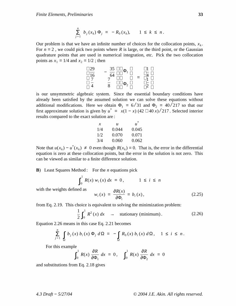
Our problem is that we have an infinite number of choices for the collocation points,xk.For n = 2 , we could pick two points whereR is large, or the third point, or the Gaussianquadrature points that are used in numerical integration, etc. Pick the two collocationpoints asx1 = 1/4 andx2 = 1/2 ; then
29
167
4
−35
647
8
Φ1
Φ2
=
1
41
2
is our unsymmetric algebraic system. Since the essential boundary conditions havealready been satisfied by the assumed solution we can solve these equations withoutadditional modifications. Here we obtainΦ1 = 6 / 31 andΦ2 = 40/ 217 so that ourfirst approximate solution is given byu* = x(1 − x) (42 + 40x) / 217 . Selected interiorresults compared to the exact solution are :
x u u*
1/4 0.044 0.0451/2 0.070 0.0713/4 0.060 0.062
Note thatu(xk) − u* (xk) ≠ 0 even thoughR(xk) = 0. That is, the error in the differentialequation is zero at these collocation points, but the error in the solution is not zero. Thiscan be viewed as similar to a finite difference solution.
B) Least Squares Method : For then equations pick
∫1
0R(x) wi (x) dx = 0 , 1 ≤ i ≤ n
with the weights defined as(2.25)wi (x) =
∂R(x)
∂Φi= bi (x) ,
from Eq. 2.19. This choice is equivalent to solving the minimization problem:
(2.26)1
2 ∫1
0R2 (x) dx → stationary (minimum) .
Equation 2.26 means in this case Eq. 2.21 becomesn
j= 1Σ
Ω∫ bj (x) bi (x) Φ j dΩ = −
Ω∫ R0 (x) bi (x) dΩ , 1 ≤ i ≤ n .
For this example
∫1
0R(x)
∂R
∂Φ1dx = 0 , ∫
1
0R(x)
∂R
∂Φ2dx = 0
and substitutions from Eq. 2.18 gives
4.3 Draft− 5/27/04 © 2004 J.E. Akin. All rights reserved.
34 J. E. Akin
202
60Φ1 +
101
60Φ2 =
55
60
101
60Φ1 +
393
105Φ2 =
57
60.
It should be noted from Eqs. 2.19, 21, 25 that this procedure yields a square matrix whichis always symmetric. Solving givesΦ1 = 0. 188 ,Φ2 = 0. 170 and selected results at thethree interior points of : 0.043, 0.068, and 0.059, respectively.
C) Galerkin Method: The concept here is to make the residual error orthogonal to thefunctions associated with the spatial influence of the constants. That is, let
u* (x) = g(x) f ( x, Φi ) =n
i=1Σ hi (x) Φi .
Here thehi term defines how we hav e assumed the contribution fromΦi will vary overspace. Here forn = 2 andh1 = (x − x2) andh2 = (x2 − x3) , we set
(2.27)wi (x) ≡ hi (x)so Eq. 2.21 simplifies to
(2.28)n
j= 1Σ
Ω∫ bj (x) hi (x) Φ j dΩ = −
Ω∫ R0 (x) hi (x) dΩ , 1 ≤ i ≤ n .
and for this specific example we require
∫1
0R(x) h1 (x) dx = 0 , ∫
1
0R(x) h2 (x) dx = 0
and Eq. 2.18 yields3
10Φ1 +
3
20Φ2 =
1
12
3
20Φ1 +
13
105Φ2 =
1
20which is again symmetric (for the self-adjoint equation). Solving gives degree offreedom values ofΦ1 = 71/ 369 , Φ2 = 7 / 41 and selected results at the three interiorpoints of : 0.044, 0.070, and 0.060, respectively.
D) Method of Moments : Pick a spatial coordinate "lever arm" as a weight :
(2.29)wi (x) ≡ x(i−1)
so that in the current one-dimensional example
(2.30)∫1
0R(x) x0 dx = 0 , ∫
1
0R(x) x1 dx = 0
gives the algebraic system11
6Φ1 +
11
12Φ2 =
1
2
11
12Φ1 +
19
20Φ2 =
1
3
with the solutionΦ1 = 122/ 649 ,Φ2 = 110/ 649 and selected results at the three interior
4.3 Draft− 5/27/04 © 2004 J.E. Akin. All rights reserved.
Finite Elements, Preliminaries 35
points of : 0.043, 0.068, and 0.059, respectively. This method usually yields anunsymmetrical system. It is popular in certain physics applications.
E) Subdomain Method : For this final method we split the solution domain,Ω , into narbitrary non-overlapping subdomains,Ωk, that completely fill the space such that
(2.31)Ω =n
k =1∪ Ωk
Then we define(2.32)wk (x) ≡ 1 for x ∈ Ωk
and it is zero elsewhere. This makes the residual error vanish on each ofn differentregions. Heren = 2 , so we arbitrarily pickΩ1 = ]0, 1
2 [ andΩ2 = ] 12 , 1[. Then
(2.33)Ω1
∫ R(x) dx = 0 ,Ω2
∫ R(x) dx = 0
yields the unsymmetric algebraic system
11
12
11
12
−53
192
229
192
Φ1
Φ2
=
1
8
3
8
.
This results inΦT = [388 352]/ 2068 and selected results at the three interior pointsof : 0.043, 0.068, and 0.059, respectively.
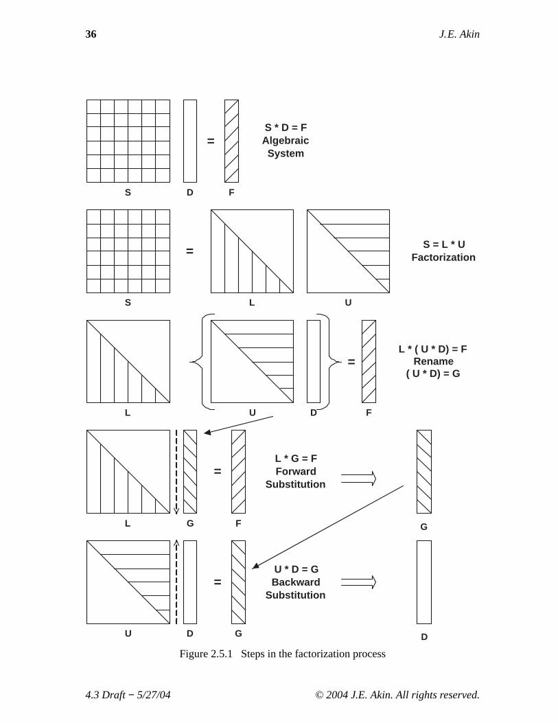
These examples show how analytical approximations can be obtained for differentialequations. These approximate methods offer some practical advantages. Instead ofsolving a differential equation we are now presented with the easier problem of solvingan algebraic problem, resulting from an integral relation, for a set of coefficients thatdefine the approximation. The weighted residual procedure is valid of any number ofspatial dimensions. The procedure is valid for any shaped domainΩ. It allows non-homogeneous coefficients. That is, the coefficient multiplying the derivatives in thedifferential operatorL can vary with location. Note that so far we have not yet made anyreferences to finite element methods. Later, you may look back on these examples asspecial cases of a single element solution. These simple examples could have beensolved with matrix inversion routines. In practice, inversions are much toocomputationally expressive, and one must solve the equations by iterative methods or bya factorization process such as the process outlined in Fig. 2.5.1. By starting with atriangular matrix the substitution processes have only one unknown per row. Thefactored triangular arrays are stored in the locations of the original square matrix.Practical implementations of direct solvers must account for sparse array storage optionsand the fact that the factorization operations increases the "fill-in" and thus the totalstorage requirement.
2.6 Boundary Condition Terms
If a boundary condition involves a non-zero value then we must extend the assumedapproximate solution to include additional constants to be used to satisfy the essentialboundary conditions. Usually these conditions are invoked prior to or during the solution
4.3 Draft− 5/27/04 © 2004 J.E. Akin. All rights reserved.
36 J. E. Akin
S * D = FAlgebraicSystem
S = L * UFactorization
L * ( U * D) = FRename
( U * D) = G
L * G = FForward
Substitution
S D F
S L U
=
G
L U
=
=
FD
L F
=
G
U D
=
G
U * D = GBackward
Substitution
D
Figure 2.5.1 Steps in the factorization process
4.3 Draft− 5/27/04 © 2004 J.E. Akin. All rights reserved.
Finite Elements, Preliminaries 37
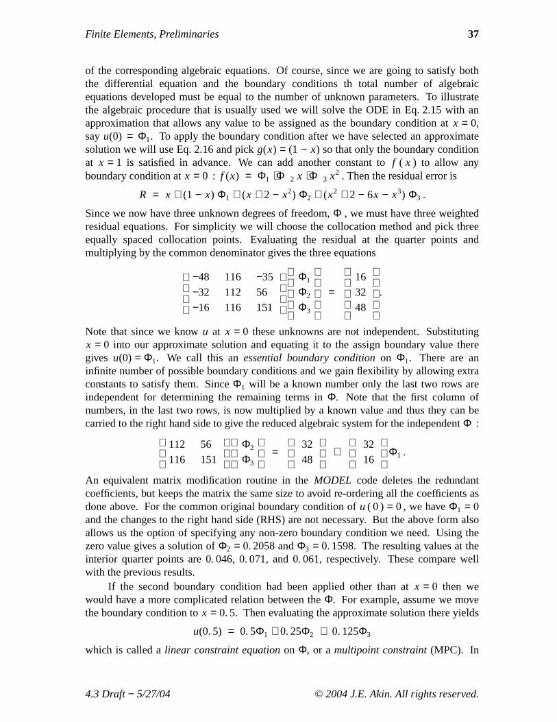
of the corresponding algebraic equations. Of course, since we are going to satisfy boththe differential equation and the boundary conditions th total number of algebraicequations developed must be equal to the number of unknown parameters. To illustratethe algebraic procedure that is usually used we will solve the ODE in Eq. 2.15 with anapproximation that allows any value to be assigned as the boundary condition atx = 0,sayu(0) = Φ1. To apply the boundary condition after we have selected an approximatesolution we will use Eq. 2.16 and pickg(x) = (1 − x) so that only the boundary conditionat x = 1 is satisfied in advance. We can add another constant tof ( x ) to allow anyboundary condition atx = 0 : f (x) = Φ1 + Φ2 x + Φ3 x2 . Then the residual error is
R = x + (1 − x) Φ1 + (x + 2 − x2) Φ2 + (x2 + 2 − 6x − x3) Φ3 .
Since we now hav e three unknown degrees of freedom,Φ , we must have three weightedresidual equations. For simplicity we will choose the collocation method and pick threeequally spaced collocation points. Evaluating the residual at the quarter points andmultiplying by the common denominator gives the three equations
−48
−32
−16
116
112
116
−35
56
151
Φ1
Φ2
Φ3
=
16
32
48
.
Note that since we knowu at x = 0 these unknowns are not independent. Substitutingx = 0 into our approximate solution and equating it to the assign boundary value theregives u(0) = Φ1. We call this anessential boundary conditionon Φ1. There are aninfinite number of possible boundary conditions and we gain flexibility by allowing extraconstants to satisfy them. SinceΦ1 will be a known number only the last two rows areindependent for determining the remaining terms inΦ. Note that the first column ofnumbers, in the last two rows, is now multiplied by a known value and thus they can becarried to the right hand side to give the reduced algebraic system for the independentΦ :
112
116
56
151
Φ2
Φ3
=
32
48
+
32
16
Φ1 .
An equivalent matrix modification routine in theMODEL code deletes the redundantcoefficients, but keeps the matrix the same size to avoid re-ordering all the coefficients asdone above. For the common original boundary condition ofu ( 0 ) = 0 , we hav eΦ1 = 0and the changes to the right hand side (RHS) are not necessary. But the above form alsoallows us the option of specifying any non-zero boundary condition we need. Using thezero value gives a solution ofΦ2 = 0. 2058 andΦ3 = 0. 1598. The resulting values at theinterior quarter points are 0. 046, 0. 071, and 0. 061, respectively. These compare wellwith the previous results.
If the second boundary condition had been applied other than atx = 0 then wewould have a more complicated relation between theΦ. For example, assume we movethe boundary condition tox = 0. 5. Then evaluating the approximate solution there yields
u(0. 5) = 0. 5Φ1 + 0. 25Φ2 + 0. 125Φ3
which is called alinear constraint equationon Φ, or amultipoint constraint(MPC). In
4.3 Draft− 5/27/04 © 2004 J.E. Akin. All rights reserved.
38 J. E. Akin
Application Dependent Software
Term / Process Required (or usekeyword example)
Optional
Differential operator, Save for flux averages
Volumetric Source
Mixed or Robin BC
Boundary Flux
Save for post-processing
Exact essential BC
Energy norm error estimate
Post-process element
APPLICATION_B_MATRIXmy_b_matrix_incELEM_SQ_MATRIX
my_el_sq_incAPPLICATION_E_MATRIX
my_e_matrix_inc
ELEM_SQ_MATRIXmy_el_sq_inc
ELEM_COL_MATRIXmy_el_col_inc
or
MIXED_SQ_MATRIXmy_mixed_sq_inc
S EK
C EQ
S Bh , C B
t
SEG_COL_MATRIXmy_seg_col_inc
EXACT_NORMAL_FLUXmy_exact_normal_flux_incC B
F
orELEM_POST_DATA
my_el_post_inc
Generate matrices
POST_PROCESS_ELEMmy_post_el_inc
APPLICATION_B_MATRIX my_b_matrix_inc
APPLICATION_E_MATRIX my_e_matrix_inc
Use an exact solution
EXACT_SOLUTIONmy_exact_inc
List exact solution
List exact fluxes
EXACT_SOLUTIONmy_exact_inc
EXACT_SOLUTION_FLUXmy_exact_flux_inc
Use exact source EXACT_SOURCEmy_exact_source_inc
, M E
ELEM_SQ_MATRIXmy_el_sq_inc
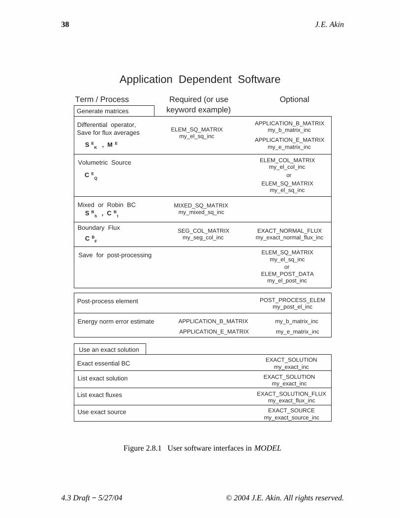
Figure 2.8.1 User software interfaces inMODEL
4.3 Draft− 5/27/04 © 2004 J.E. Akin. All rights reserved.
Finite Elements, Preliminaries 39
other words we would have to solve the weighted residual algebraic system subject to alinear constraint. This is a fairly common situation in practical design problems andadaptive analysis procedures. The computational details for enforcing the above essentialboundary conditions are discussed in detail later.
2.7 Adding More Unknowns
Since the exact solution of the model problem is not a polynomial our globalpolynomial approach can never yield an exact solution. However, we can significantlyimprove the accuracy by adding more unknown coefficients to the expansion in Eq. 2.17.In matrix notation the original global Galerkin matrices become
Se =L∫ hT b dx , Ce = −
L∫ hT Q(x) dx
whereQ(x) = x is the source term,b = h′′ + h comes from the differential operatoracting onu, and where a prime denotes a derivative. Likewise, using Least Squares:
Se =L∫ bT b dx , Ce =
L∫ bT Q(x) dx
Here we see that the Least Squares square matrix will always be symmetric, but theGalerkin form may not be. As we add more unknown coefficients we just increase thesize of the functions inh, and thus inb, and increase the number of integration points toaccount for the higher degree polynomials occurring in the matrices. A disadvantage ofadding more unknowns to a global solution is that the unknown parameters are fullycoupled to each other. That means the algebraic equations to be solved are fullypopulated, and thus very expensive to solve. The finite element method will lead to verysparse equations that are efficient to solve.
2.8 Numerical Integration
Since numerical integration simply replaces an integral with a special summationthis approach has the potential for automating all the above integrals required by theMWR. Then we can include thousands of unknown coefficients,Φi , in our test solution.Here we are dealing with polynomials. It is well known that in one-dimension Gaussianquadrature withnq terms will exactly integrate a polynomial of order (2nq − 1). Gaussproved that this is the minimum number of points that can be used in a summation toyield the exact results. Therefore, it is the most efficient method available for integratingpolynomials. Thus, we could replace the above integrals with a two-point Gauss rule.(This will be considered in full detail later in Sec. 4.4, and Table 4.2.) For example, theGalerkin source term is
(2.34)Ce1 = ∫
1
0x h1 (x) dx =
nq
j=1Σ x j h1 (x j ) wj
where thex j and wj are tabulated data. Fornq = 2 on the domainΩ = ]0, 1[ we hav ew1 = w2 = 1 / 2 andx j = (1 ± 1 / √3 ) / 2, or x1 = 0. 2113325 andx2 = 0. 788675. So
4.3 Draft− 5/27/04 © 2004 J.E. Akin. All rights reserved.
40 J. E. Akin
∫1
0x ( x − x2 ) dx =
nq
j=1Σ ( x2
j − x3j ) wj =
2
j=1Σ x2
j ( 1 − x j ) wj
= [ (0. 2113248)2 (0. 7886751) 1/2+ (0. 7886751)2 (0. 2113248) 1/2 ]
= (0. 16666667) 1/2 = 0. 083333 .
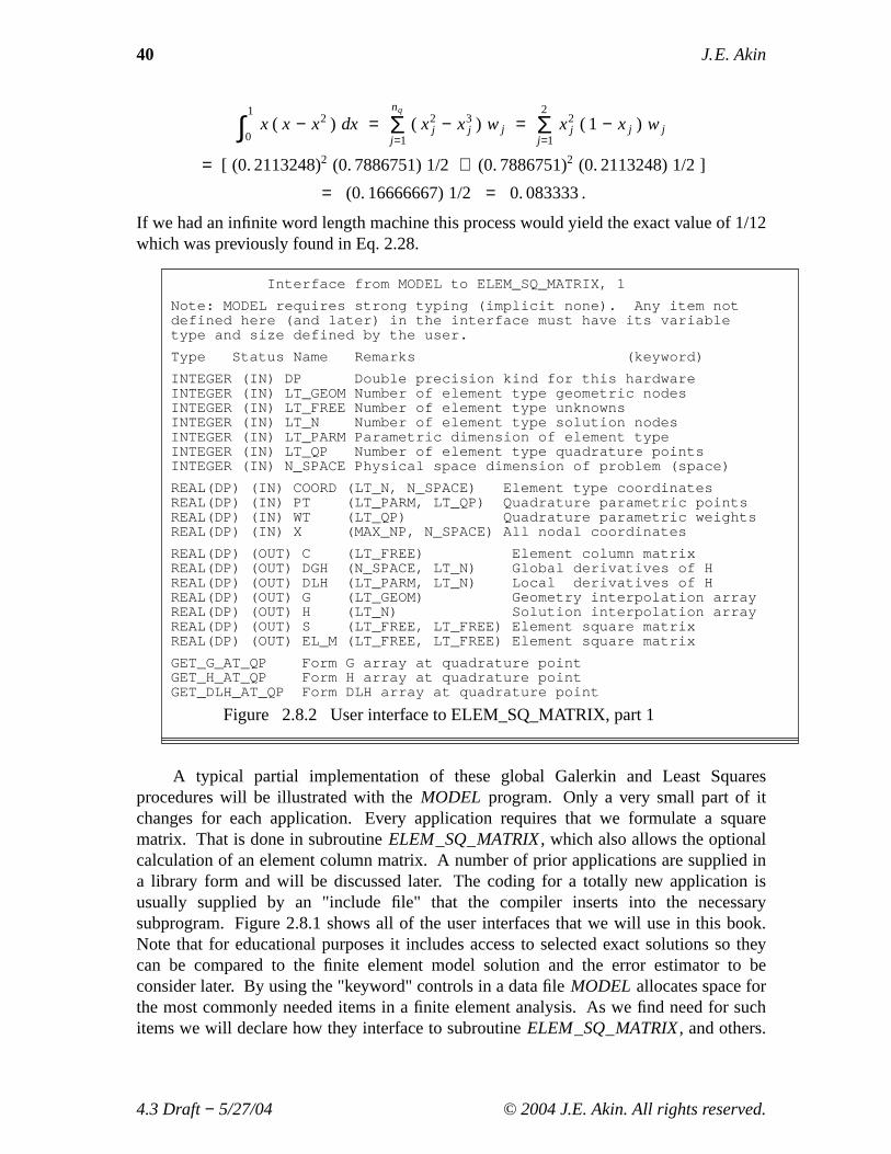
If we had an infinite word length machine this process would yield the exact value of 1/12which was previously found in Eq. 2.28.
Interface from MODEL to ELEM_SQ_MATRIX, 1
Note: MODEL requires strong typing (implicit none). Any item notdefined here (and later) in the interface must have its variabletype and size defined by the user.
Type Status Name Remarks (keyword)
INTEGER (IN) DP Double precision kind for this hardwareINTEGER (IN) LT_GEOM Number of element type geometric nodesINTEGER (IN) LT_FREE Number of element type unknownsINTEGER (IN) LT_N Number of element type solution nodesINTEGER (IN) LT_PARM Parametric dimension of element typeINTEGER (IN) LT_QP Number of element type quadrature pointsINTEGER (IN) N_SPACE Physical space dimension of problem (space)
REAL(DP) (IN) COORD (LT_N, N_SPACE) Element type coordinatesREAL(DP) (IN) PT (LT_PARM, LT_QP) Quadrature parametric pointsREAL(DP) (IN) WT (LT_QP) Quadrature parametric weightsREAL(DP) (IN) X (MAX_NP, N_SPACE) All nodal coordinates
REAL(DP) (OUT) C (LT_FREE) Element column matrixREAL(DP) (OUT) DGH (N_SPACE, LT_N) Global derivatives of HREAL(DP) (OUT) DLH (LT_PARM, LT_N) Local derivatives of HREAL(DP) (OUT) G (LT_GEOM) Geometry interpolation arrayREAL(DP) (OUT) H (LT_N) Solution interpolation arrayREAL(DP) (OUT) S (LT_FREE, LT_FREE) Element square matrixREAL(DP) (OUT) EL_M (LT_FREE, LT_FREE) Element square matrix
GET_G_AT_QP Form G array at quadrature pointGET_H_AT_QP Form H array at quadrature pointGET_DLH_AT_QP Form DLH array at quadrature point
Figure 2.8.2 User interface to ELEM_SQ_MATRIX, part 1
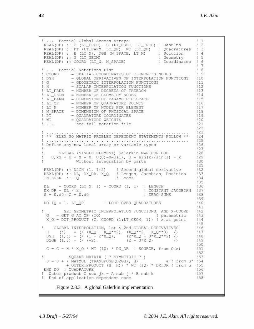
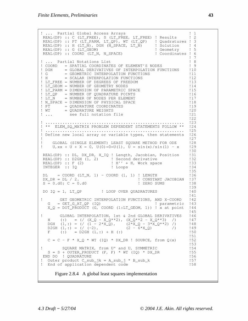
A typical partial implementation of these global Galerkin and Least Squaresprocedures will be illustrated with theMODEL program. Only a very small part of itchanges for each application. Every application requires that we formulate a squarematrix. That is done in subroutineELEM_SQ_MATRIX, which also allows the optionalcalculation of an element column matrix. A number of prior applications are supplied ina library form and will be discussed later. The coding for a totally new application isusually supplied by an "include file" that the compiler inserts into the necessarysubprogram. Figure 2.8.1 shows all of the user interfaces that we will use in this book.Note that for educational purposes it includes access to selected exact solutions so theycan be compared to the finite element model solution and the error estimator to beconsider later. By using the "keyword" controls in a data fileMODEL allocates space forthe most commonly needed items in a finite element analysis. As we find need for suchitems we will declare how they interface to subroutineELEM_SQ_MATRIX, and others.
4.3 Draft− 5/27/04 © 2004 J.E. Akin. All rights reserved.
Finite Elements, Preliminaries 41
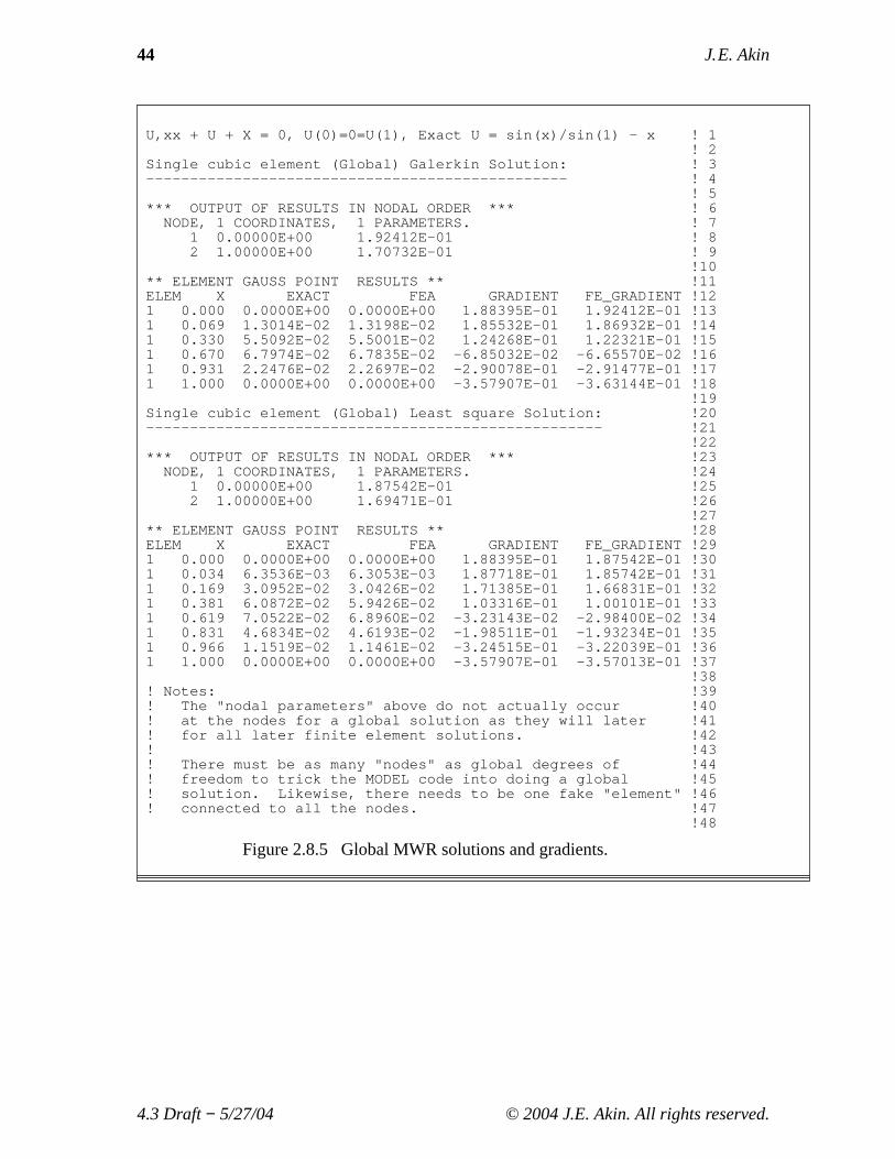
Figure 2.8.2 lists the portion of the interface that will be used here. The coding of theabove problems, by numerical integration, are shown in Figs. 2.8.3 and 2.8.4,respectively. The results agree well, as do all of our weighted residual solutions. Theglobal Galerkin and Least Squares results are listed in Fig. 2.8.5. Plotting the resultingsolutions shows very similar curves from all five approaches to the MWR.
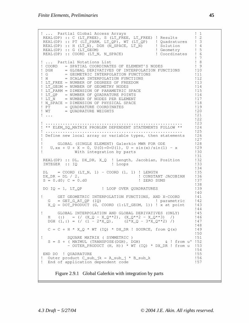
2.9 Integration By Parts
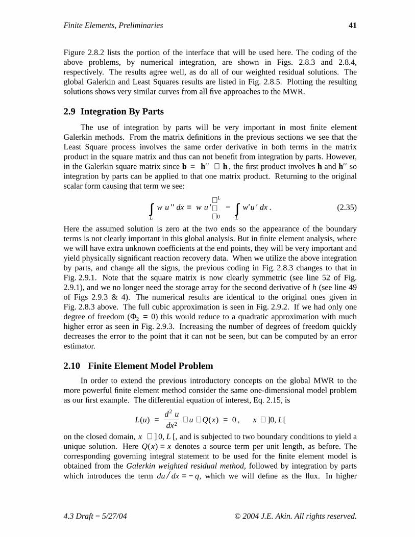
The use of integration by parts will be very important in most finite elementGalerkin methods. From the matrix definitions in the previous sections we see that theLeast Square process involves the same order derivative in both terms in the matrixproduct in the square matrix and thus can not benefit from integration by parts. However,in the Galerkin square matrix sinceb = h′′ + h , the first product involvesh andh′′ sointegration by parts can be applied to that one matrix product. Returning to the originalscalar form causing that term we see:
(2.35)L∫ w u ′′ dx = w u ′
L
0
−L∫ w′u ′ dx .
Here the assumed solution is zero at the two ends so the appearance of the boundaryterms is not clearly important in this global analysis. But in finite element analysis, wherewe will have extra unknown coefficients at the end points, they will be very important andyield physically significant reaction recovery data. When we utilize the above integrationby parts, and change all the signs, the previous coding in Fig. 2.8.3 changes to that inFig. 2.9.1. Note that the square matrix is now clearly symmetric (see line 52 of Fig.2.9.1), and we no longer need the storage array for the second derivative ofh (see line 49of Figs 2.9.3 & 4). The numerical results are identical to the original ones given inFig. 2.8.3 above. The full cubic approximation is seen in Fig. 2.9.2. If we had only onedegree of freedom (Φ2 = 0) this would reduce to a quadratic approximation with muchhigher error as seen in Fig. 2.9.3. Increasing the number of degrees of freedom quicklydecreases the error to the point that it can not be seen, but can be computed by an errorestimator.
2.10 Finite Element Model Problem
In order to extend the previous introductory concepts on the global MWR to themore powerful finite element method consider the same one-dimensional model problemas our first example. The differential equation of interest, Eq. 2.15, is
L(u) =d2 u
dx2+ u + Q(x) = 0 , x ∈ ]0, L[
on the closed domain,x ∈ ] 0, L [, and is subjected to two boundary conditions to yield aunique solution. HereQ(x) = x denotes a source term per unit length, as before. Thecorresponding governing integral statement to be used for the finite element model isobtained from theGalerkin weighted residual method, followed by integration by partswhich introduces the termdu/ dx = − q, which we will define as the flux. In higher
4.3 Draft− 5/27/04 © 2004 J.E. Akin. All rights reserved.
42 J. E. Akin
! ... Partial Global Access Arrays ! 1REAL(DP) :: C (LT_FREE), S (LT_FREE, LT_FREE) ! Results ! 2REAL(DP) :: PT (LT_PARM, LT_QP), WT (LT_QP) ! Quadratures ! 3REAL(DP) :: H (LT_N), DGH (N_SPACE, LT_N) ! Solution ! 4REAL(DP) :: G (LT_GEOM) ! Geometry ! 5REAL(DP) :: COORD (LT_N, N_SPACE) ! Coordinates ! 6
! 7! ... Partial Notations List ! 8! COORD = SPATIAL COORDINATES OF ELEMENT’S NODES ! 9! DGH = GLOBAL DERIVATIVES OF INTERPOLATION FUNCTIONS !10! G = GEOMETRIC INTERPOLATION FUNCTIONS !11! H = SCALAR INTERPOLATION FUNCTIONS !12! LT_FREE = NUMBER OF DEGREES OF FREEDOM !13! LT_GEOM = NUMBER OF GEOMETRY NODES !14! LT_PARM = DIMENSION OF PARAMETRIC SPACE !15! LT_QP = NUMBER OF QUADRATURE POINTS !16! LT_N = NUMBER OF NODES PER ELEMENT !17! N_SPACE = DIMENSION OF PHYSICAL SPACE !18! PT = QUADRATURE COORDINATES !19! WT = QUADRATURE WEIGHTS !20! ... see full notation file !21
!22! ......................................................... !23! ** ELEM_SQ_MATRIX PROBLEM DEPENDENT STATEMENTS FOLLOW ** !24! ......................................................... !25! Define any new local array or variable types !26! !27! GLOBAL (SINGLE ELEMENT) Galerkin MWR FOR ODE !28! U,xx + U + X = 0, U(0)=0=U(1), U = sin(x)/sin(1) - x !29! Without integration by parts !30
!31REAL(DP) :: D2GH (1, 1:2) ! Second global derivative !32REAL(DP) :: DL, DX_DR, X_Q ! Length, Jacobian, Position !33INTEGER :: IQ ! Loops !34
!35DL = COORD (LT_N, 1) - COORD (1, 1) ! LENGTH !36DX_DR = DL / 2. ! CONSTANT JACOBIAN !37S = 0.d0; C = 0.d0 ! ZERO SUMS !38
!39DO IQ = 1, LT_QP ! LOOP OVER QUADRATURES !40
!41! GET GEOMETRIC INTERPOLATION FUNCTIONS, AND X-COORD !42
G = GET_G_AT_QP (IQ) ! parametric !43X_Q = DOT_PRODUCT (G, COORD (1:LT_GEOM, 1)) ! x at point !44
!45! GLOBAL INTERPOLATION, 1st & 2nd GLOBAL DERIVATIVES !46
H (:) = (/ (X_Q - X_Q**2), (X_Q**2 - X_Q**3) /) !47DGH (1,:) = (/ (1 - 2*X_Q), (2*X_Q - 3*X_Q**2) /) !48D2GH (1,:) = (/ (-2), (2 - 3*X_Q) /) !49
!50C = C - H * X_Q * WT (IQ) * DX_DR ! SOURCE, from Q(x) !51
!52! SQUARE MATRIX ( ? SYMMETRIC ? ) !53
S = S + ( MATMUL (TRANSPOSE(D2GH), H) & ! from u" !54+ OUTER_PRODUCT (H, H)) * WT (IQ) * DX_DR ! from u !55
END DO ! QUADRATURE !56! Outer product C_sub_jk = A_sub_j * B_sub_k !57! End of application dependent code !58
Figure 2.8.3 A global Galerkin implementation
4.3 Draft− 5/27/04 © 2004 J.E. Akin. All rights reserved.
Finite Elements, Preliminaries 43
! ... Partial Global Access Arrays ! 1REAL(DP) :: C (LT_FREE), S (LT_FREE, LT_FREE) ! Results ! 2REAL(DP) :: PT (LT_PARM, LT_QP), WT (LT_QP) ! Quadratures ! 3REAL(DP) :: H (LT_N), DGH (N_SPACE, LT_N) ! Solution ! 4REAL(DP) :: G (LT_GEOM) ! Geometry ! 5REAL(DP) :: COORD (LT_N, N_SPACE) ! Coordinates ! 6
! 7! ... Partial Notations List ! 8! COORD = SPATIAL COORDINATES OF ELEMENT’S NODES ! 9! DGH = GLOBAL DERIVATIVES OF INTERPOLATION FUNCTIONS !10! G = GEOMETRIC INTERPOLATION FUNCTIONS !11! H = SCALAR INTERPOLATION FUNCTIONS !12! LT_FREE = NUMBER OF DEGREES OF FREEDOM !13! LT_GEOM = NUMBER OF GEOMETRY NODES !14! LT_PARM = DIMENSION OF PARAMETRIC SPACE !15! LT_QP = NUMBER OF QUADRATURE POINTS !16! LT_N = NUMBER OF NODES PER ELEMENT !17! N_SPACE = DIMENSION OF PHYSICAL SPACE !18! PT = QUADRATURE COORDINATES !19! WT = QUADRATURE WEIGHTS !20! ... see full notation file !21
!22! ......................................................... !23! ** ELEM_SQ_MATRIX PROBLEM DEPENDENT STATEMENTS FOLLOW ** !24! ......................................................... !25! Define new local array or variable types, then statements !26! !27! GLOBAL (SINGLE ELEMENT) LEAST SQUARE METHOD FOR ODE !28! U,xx + U + X = 0, U(0)=0=U(1), U = sin(x)/sin(1) - x !29
!30REAL(DP) :: DL, DX_DR, X_IQ ! Length, Jacobian, Position !31REAL(DP) :: D2GH (1, 2) ! Second derivative !32REAL(DP) :: F (2) ! H’’ + H, Work space !33INTEGER :: IQ ! Loops !34
!35DL = COORD (LT_N, 1) - COORD (1, 1) ! LENGTH !36DX_DR = DL / 2. ! CONSTANT JACOBIAN !37S = 0.d0; C = 0.d0 ! ZERO SUMS !38
!39DO IQ = 1, LT_QP ! LOOP OVER QUADRATURES !40
!41! GET GEOMETRIC INTERPOLATION FUNCTIONS, AND X-COORD !42
G = GET_G_AT_QP (IQ) ! parametric !43X_Q = DOT_PRODUCT (G, COORD (1:LT_GEOM, 1)) ! x at point !44
!45! GLOBAL INTERPOLATION, 1st & 2nd GLOBAL DERIVATIVES !46
H (:) = (/ (X_Q - X_Q**2), (X_Q**2 - X_Q**3) /) !47DGH (1,:) = (/ (1 - 2*X_Q), (2*X_Q - 3*X_Q**2) /) !48D2GH (1,:) = (/ (-2), (2 - 6*X_Q) /) !49F (:) = D2GH (1,:) + H (:) !50
!51C = C - F * X_Q * WT (IQ) * DX_DR ! SOURCE, from Q(x) !52
!53! SQUARE MATRIX, from U" and U, SYMMETRIC !54
S = S + OUTER_PRODUCT (F, F) * WT (IQ) * DX_DR !55END DO ! QUADRATURE !56
! Outer product C_sub_jk = A_sub_j * B_sub_k !57! End of application dependent code !58
Figure 2.8.4 A global least squares implementation
4.3 Draft− 5/27/04 © 2004 J.E. Akin. All rights reserved.
44 J. E. Akin
U,xx + U + X = 0, U(0)=0=U(1), Exact U = sin(x)/sin(1) - x ! 1! 2
Single cubic element (Global) Galerkin Solution: ! 3------------------------------------------------ ! 4
! 5*** OUTPUT OF RESULTS IN NODAL ORDER *** ! 6
NODE, 1 COORDINATES, 1 PARAMETERS. ! 71 0.00000E+00 1.92412E-01 ! 82 1.00000E+00 1.70732E-01 ! 9
!10** ELEMENT GAUSS POINT RESULTS ** !11ELEM X EXACT FEA GRADIENT FE_GRADIENT !121 0.000 0.0000E+00 0.0000E+00 1.88395E-01 1.92412E-01 !131 0.069 1.3014E-02 1.3198E-02 1.85532E-01 1.86932E-01 !141 0.330 5.5092E-02 5.5001E-02 1.24268E-01 1.22321E-01 !151 0.670 6.7974E-02 6.7835E-02 -6.85032E-02 -6.65570E-02 !161 0.931 2.2476E-02 2.2697E-02 -2.90078E-01 -2.91477E-01 !171 1.000 0.0000E+00 0.0000E+00 -3.57907E-01 -3.63144E-01 !18
!19Single cubic element (Global) Least square Solution: !20---------------------------------------------------- !21
!22*** OUTPUT OF RESULTS IN NODAL ORDER *** !23
NODE, 1 COORDINATES, 1 PARAMETERS. !241 0.00000E+00 1.87542E-01 !252 1.00000E+00 1.69471E-01 !26
!27** ELEMENT GAUSS POINT RESULTS ** !28ELEM X EXACT FEA GRADIENT FE_GRADIENT !291 0.000 0.0000E+00 0.0000E+00 1.88395E-01 1.87542E-01 !301 0.034 6.3536E-03 6.3053E-03 1.87718E-01 1.85742E-01 !311 0.169 3.0952E-02 3.0426E-02 1.71385E-01 1.66831E-01 !321 0.381 6.0872E-02 5.9426E-02 1.03316E-01 1.00101E-01 !331 0.619 7.0522E-02 6.8960E-02 -3.23143E-02 -2.98400E-02 !341 0.831 4.6834E-02 4.6193E-02 -1.98511E-01 -1.93234E-01 !351 0.966 1.1519E-02 1.1461E-02 -3.24515E-01 -3.22039E-01 !361 1.000 0.0000E+00 0.0000E+00 -3.57907E-01 -3.57013E-01 !37
!38! Notes: !39! The "nodal parameters" above do not actually occur !40! at the nodes for a global solution as they will later !41! for all later finite element solutions. !42! !43! There must be as many "nodes" as global degrees of !44! freedom to trick the MODEL code into doing a global !45! solution. Likewise, there needs to be one fake "element" !46! connected to all the nodes. !47
!48
Figure 2.8.5 Global MWR solutions and gradients.
4.3 Draft− 5/27/04 © 2004 J.E. Akin. All rights reserved.
Finite Elements, Preliminaries 45
! ... Partial Global Access Arrays ! 1REAL(DP) :: C (LT_FREE), S (LT_FREE, LT_FREE) ! Results ! 2REAL(DP) :: PT (LT_PARM, LT_QP), WT (LT_QP) ! Quadratures ! 3REAL(DP) :: H (LT_N), DGH (N_SPACE, LT_N) ! Solution ! 4REAL(DP) :: G (LT_GEOM) ! Geometry ! 5REAL(DP) :: COORD (LT_N, N_SPACE) ! Coordinates ! 6
! 7! ... Partial Notations List ! 8! COORD = SPATIAL COORDINATES OF ELEMENT’S NODES ! 9! DGH = GLOBAL DERIVATIVES OF INTERPOLATION FUNCTIONS !10! G = GEOMETRIC INTERPOLATION FUNCTIONS !11! H = SCALAR INTERPOLATION FUNCTIONS !12! LT_FREE = NUMBER OF DEGREES OF FREEDOM !13! LT_GEOM = NUMBER OF GEOMETRY NODES !14! LT_PARM = DIMENSION OF PARAMETRIC SPACE !15! LT_QP = NUMBER OF QUADRATURE POINTS !16! LT_N = NUMBER OF NODES PER ELEMENT !17! N_SPACE = DIMENSION OF PHYSICAL SPACE !18! PT = QUADRATURE COORDINATES !19! WT = QUADRATURE WEIGHTS !20! ... !21
!22! ........................................................ !23! ** ELEM_SQ_MATRIX PROBLEM DEPENDENT STATEMENTS FOLLOW ** !24! ........................................................ !25! Define new local array or variable types, then statements !26! !27! GLOBAL (SINGLE ELEMENT) Galerkin MWR FOR ODE !28! U,xx + U + X = 0, U(0)=0=U(1), U = sin(x)/sin(1) - x !29! With integration by parts !30
!31REAL(DP) :: DL, DX_DR, X_Q ! Length, Jacobian, Position !32INTEGER :: IQ ! Loops !33
!34DL = COORD (LT_N, 1) - COORD (1, 1) ! LENGTH !35DX_DR = DL / 2. ! CONSTANT JACOBIAN !36S = 0.d0; C = 0.d0 ! ZERO SUMS !37
!38DO IQ = 1, LT_QP ! LOOP OVER QUADRATURES !39
!40! GET GEOMETRIC INTERPOLATION FUNCTIONS, AND X-COORD !41
G = GET_G_AT_QP (IQ) ! parametric !42X_Q = DOT_PRODUCT (G, COORD (1:LT_GEOM, 1)) ! x at point !43
!44! GLOBAL INTERPOLATION AND GLOBAL DERIVATIVES (ONLY) !45
H (:) = (/ (X_Q - X_Q**2), (X_Q**2 - X_Q**3) /) !46DGH (1,:) = (/ (1 - 2*X_Q), (2*X_Q - 3*X_Q**2) /) !47
!48C = C + H * X_Q * WT (IQ) * DX_DR ! SOURCE, from Q(x) !49
!50! SQUARE MATRIX ( SYMMETRIC ) !51
S = S + ( MATMUL (TRANSPOSE(DGH), DGH) & ! from u" !52- OUTER_PRODUCT (H, H)) * WT (IQ) * DX_DR ! from u !53
!54END DO ! QUADRATURE !55
! Outer product C_sub_jk = A_sub_j * B_sub_k !56! End of application dependent code !57
Figure 2.9.1 Global Galerkin with integration by parts
4.3 Draft− 5/27/04 © 2004 J.E. Akin. All rights reserved.

46 J. E. Akin
0 0.1 0.2 0.3 0.4 0.5 0.6 0.7 0.8 0.9 10
0.01
0.02
0.03
0.04
0.05
0.06
0.07
0.08Cubic Global Galerkin, by parts, u"+u+x=0, u(0)=0=u(1)
X
u, *
= F
EA
app
roxi
mat
ion
Figure 2.9.2 Exact (-) and cubic global Galerkin (*) solutions
0 0.1 0.2 0.3 0.4 0.5 0.6 0.7 0.8 0.9 10
0.01
0.02
0.03
0.04
0.05
0.06
0.07
0.08Quadratic Global Galerkin, by parts, u"+u+x=0, u(0)=0=u(1)
X
u, o
= F
EA
app
roxi
mat
ion
Figure 2.9.3 Exact (-) and quadratic global Galerkin (o) solutions
4.3 Draft− 5/27/04 © 2004 J.E. Akin. All rights reserved.
Finite Elements, Preliminaries 47
dimension problems it is the flux vector,q. On a boundary we may be interested in arelated scalar term,qn = q .n, which is the flux normal to the boundary defined by theunit normal vectorn. For the special case of the one-dimensional form being consideredhere we need to note that at the left limit of the domainn = − 1 i while at the right limit itis n = + 1 i. In this case, the Galerkin method states that the function,v, that satisfies theboundary conditions and the integral form:
(2.36)I = ∫L
0[dw
dx
du
dx− w u − w Q ] dx + q0 u ( 0 ) − qL u ( L ) = 0 ,
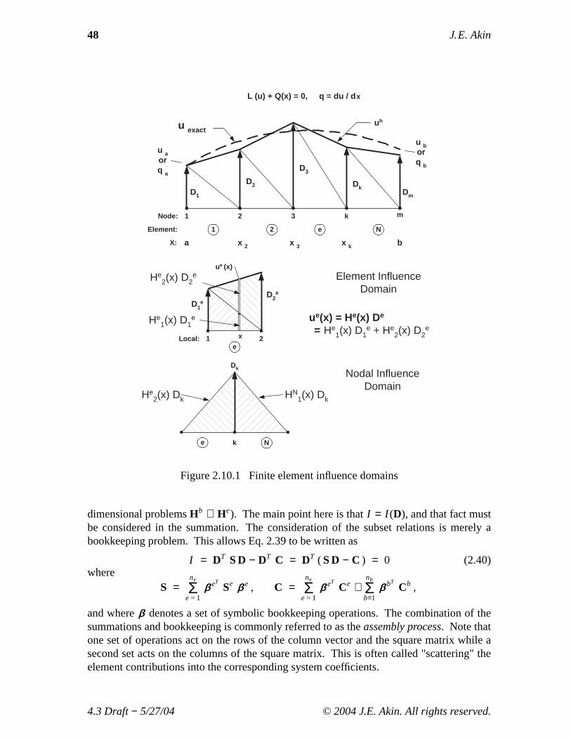
also satisfies Eq. 2.15. For a finite element model we must generate a mesh thatsubdivides the domain and (usually) its boundary. The unknown coefficients in the finiteelement model,D, will be assigned to the node points of the mesh. Within each elementthe solution will be approximated by an assumed local spatial behavior. That in turndefines the assumptions for spatial derivatives in an element domain. To illustrate this inone-dimension consider Fig. 2.10.1 which compares an exact solution (dashed) and apiecewise linear finite element model. The domains of influence of a typical element anda typical node are sketched there. In a finite element model,I is assumed to be the sumof thene element andnb boundary segment contributions so that
(2.37)I =ne
e=1Σ I e +
nb
b=1Σ I b ,
where herenb = 2 and consists of the last two terms given in Eq. 2.36. A typical elementterm is
(2.38)I e =Le∫
( due / dx )2 − (ue)2 − Qe ue
dx ,
whereLe is the length of the element. To evaluate such a typical element contribution, itis necessary to introduce a set of interpolation functions,H, soue(x) = He(x) De, and
due / dx = dHe / dx De = DeTdHeT / dx ,
whereDe denotes the nodal values ofu for elemente. One of the few standard notationsin finite element analysis is to denote the result of the differential operator acting on theinterpolation functions,H, by the symbolB. That is,Be ≡ d He / dx. Thus, a typicalelement contribution is
(2.39)I e = DeTSe De − DeT
Ce ,
with Se = (Se1 − Se
2) and where the first contribution to the square matrix is
Se1 ≡
Le∫
dHeT
dx
dHe
dxdx =
Le∫ BeT
Be dx ,
which, for this linear element, has a constant integrand and can be integrated byinspection. The second square matrix contribution and the resultant source vector are:
Se2 ≡
Le∫ HeT
He dx , Ce ≡Le∫ Qe HeT
dx .
Clearly, both the element degrees of freedom,De, and the boundary degrees of freedom,Db, are subsets of the total vector of unknown parameters,D. That is, De ⊆ D andDb ⊂ D. Of course, theDb are usually a subset of theDe ( i.e., Db ⊂ De and in higher
4.3 Draft− 5/27/04 © 2004 J.E. Akin. All rights reserved.
48 J. E. Akin
L (u) + Q(x) = 0, q = du / d x
D1
D2
D3
DkDm
u aorq a
u borq b
1 2 3 k mNode:
Element: 1 2 e N
D1e
D2e
ue (x)
x1 2e
Element InfluenceDomain
ue(x) = He(x) De
= He1(x) D1
e + He2(x) D2
e
He2(x) D2
e
He1(x) D1
e
e k N
He2(x) Dk HN
1(x) Dk
DkNodal Influence
Domain
u exactuh
X: a bx kx 2 x 3
Local:
Figure 2.10.1 Finite element influence domains
dimensional problemsHb ⊂ He). The main point here is thatI = I (D), and that fact mustbe considered in the summation. The consideration of the subset relations is merely abookkeeping problem. This allows Eq. 2.39 to be written as
(2.40)I = DT S D − DT C = DT ( S D − C ) = 0where
S =ne
e = 1Σ ββ eT
Se ββ e , C =ne
e = 1Σ ββ eT
Ce +nb
b=1Σ ββ bT
Cb ,
and whereββ denotes a set of symbolic bookkeeping operations. The combination of thesummations and bookkeeping is commonly referred to as theassembly process. Note thatone set of operations act on the rows of the column vector and the square matrix while asecond set acts on the columns of the square matrix. This is often called "scattering" theelement contributions into the corresponding system coefficients.
4.3 Draft− 5/27/04 © 2004 J.E. Akin. All rights reserved.
Finite Elements, Preliminaries 49
It is easily shown that for a non-trivial solution,D ≠ O, we must haveO = S D − C,as the governing algebraic equations to be solved for the unknown nodal parameters,D.To be specific, consider a linear interpolation element with two nodes per element,(nn = 2). If the element length isLe = (x2 − x1)
e, then the element interpolation, writtenin physical coordinates, is
He(x) =
(x2e − x)
Le
(x − x1e)
Le
,
so that
Be =dHe
dx=
−1
Le
1
Le
.
Therefore, the two parts (diffusion and convection) to the element square matrix are
(2.41)Se1 =
1
Le
1
−1
−1
1
, Se
2 =Le
6
2
1
1
2
,
while the element column (source) matrix is
Ce =Le∫ HeT
Qedx =Le∫
Qe
Le
(x2e − x)
(x − x1e)
d x .
If we were to assume thatQ = Q0, a constant, the constant source would simplify toCeT
= 1 1 Q0 Le / 2. That is, the finite element model would replace the constantsource per unit length by lumping half its resultant,Q0 Le, at each of the two nodes of theelement. In the given case ofQ(x) = x, the source vector reduces to
(2.42)Ce =Le
6
2
1
1
2
Q1
Q2
,
whereQ1 = x1 andQ2 = x2 are the nodal values of the source. The latter form is whatresults if we make the usual assumption that spatially varying data are to be input at thesystem nodes and interpolated inside the element. In other words, it is common tointerpolate from gathered nodal data to defineQ(x) = He(x)Qe whereQe are the localnodal values of the source. Then the resulting integral is the same as inSe
2, soCe = Se
2Qe as given above. If we setQ1 = Q2 = Q0 this agrees with the constant source
resultant, as noted above.These are all the arrays needed to carry out an analysis if no post-processing
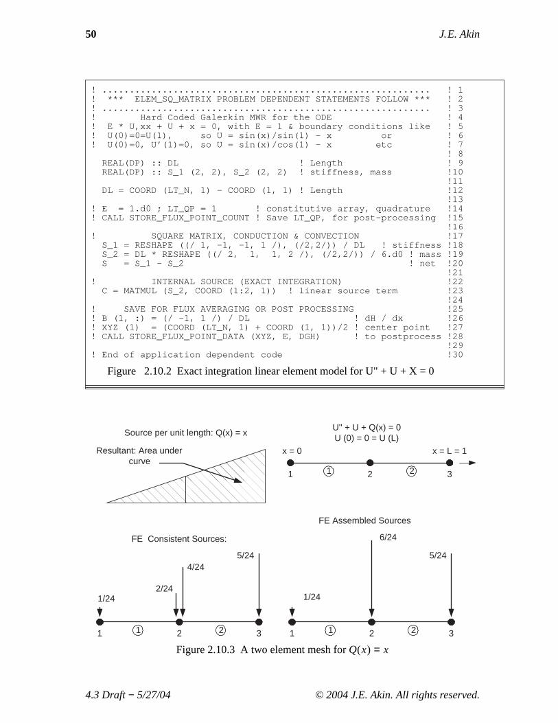
information is needed. Thus it is relatively easy to hard-code the source for this modelproblem. Figure 2.10.2 gives such an implementation as well as including commentstatements that look ahead to saving data typically needed for post-processing operationsto be introduced later. The element square matrices are defined at lines 18-20 and thematrix multiplication to formCe is carried out at line 23, using the nodal values ofxwhich happens in this example to be the nodal values ofQ(x). Two optional lines appearas comments at lines 15 and 28. They can be used to save data that can be used later inan error estimate or post-processing. Alternatively, those data could simply be re-computed in a later phase of the program.
4.3 Draft− 5/27/04 © 2004 J.E. Akin. All rights reserved.
50 J. E. Akin
! ............................................................ ! 1! *** ELEM_SQ_MATRIX PROBLEM DEPENDENT STATEMENTS FOLLOW *** ! 2! ............................................................ ! 3! Hard Coded Galerkin MWR for the ODE ! 4! E * U,xx + U + x = 0, with E = 1 & boundary conditions like ! 5! U(0)=0=U(1), s o U = sin(x)/sin(1) - x or ! 6! U(0)=0, U’(1)=0, so U = sin(x)/cos(1) - x etc ! 7
! 8REAL(DP) :: DL ! Length ! 9REAL(DP) :: S_1 (2, 2), S_2 (2, 2) ! stiffness, mass !10
!11DL = COORD (LT_N, 1) - COORD (1, 1) ! Length !12
!13! E = 1.d0 ; LT_QP = 1 ! constitutive array, quadrature !14! CALL STORE_FLUX_POINT_COUNT ! Save LT_QP, for post-processing !15
!16! SQUARE MATRIX, CONDUCTION & CONVECTION !17
S_1 = RESHAPE ((/ 1, -1, -1, 1 /), (/2,2/)) / DL ! stiffness !18S_2 = DL * RESHAPE ((/ 2, 1, 1, 2 /), (/2,2/)) / 6.d0 ! mass !19S = S_1 - S_2 ! net !20
!21! INTERNAL SOURCE (EXACT INTEGRATION) !22
C = MATMUL (S_2, COORD (1:2, 1)) ! linear source term !23!24
! SAVE FOR FLUX AVERAGING OR POST PROCESSING !25! B (1, :) = (/ -1, 1 /) / DL ! dH / dx !26! XYZ (1) = (COORD (LT_N, 1) + COORD (1, 1))/2 ! center point !27! CALL STORE_FLUX_POINT_DATA (XYZ, E, DGH) ! to postprocess !28
!29! End of application dependent code !30
Figure 2.10.2 Exact integration linear element model for U" + U + X = 0
U'' + U + Q(x) = 0U (0) = 0 = U (L)
x = 0 x = L = 1
1 2 31 2
Source per unit length: Q(x) = x
Resultant: Area undercurve
1 2 31 2
FE Consistent Sources:
1/242/24
4/245/24
1 2 31 2
1/24
5/24
6/24
FE Assembled Sources
Figure 2.10.3 A two element mesh forQ(x) = x
4.3 Draft− 5/27/04 © 2004 J.E. Akin. All rights reserved.
Finite Elements, Preliminaries 51
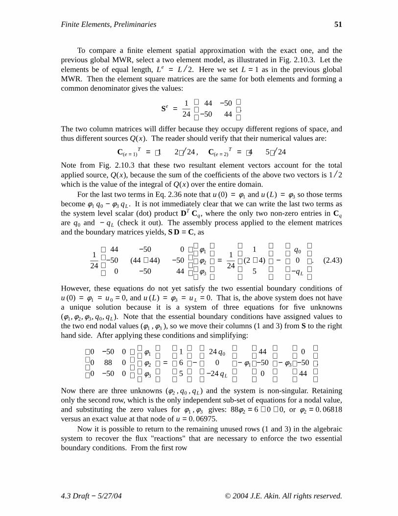
To compare a finite element spatial approximation with the exact one, and theprevious global MWR, select a two element model, as illustrated in Fig. 2.10.3. Let theelements be of equal length,Le = L / 2. Here we setL = 1 as in the previous globalMWR. Then the element square matrices are the same for both elements and forming acommon denominator gives the values:
Se =1
24
44
−50
−50
44
.
The two column matrices will differ because they occupy different regions of space, andthus different sourcesQ(x). The reader should verify that their numerical values are:
C(e = 1)T = 1 2 / 24, C(e = 2)
T = 4 5 / 24
Note from Fig. 2.10.3 that these two resultant element vectors account for the totalapplied source,Q(x), because the sum of the coefficients of the above two vectors is 1/ 2which is the value of the integral ofQ(x) over the entire domain.
For the last two terms in Eq. 2.36 note thatu (0) = φ1 andu (L) = φ3 so those termsbecomeφ1 q0 − φ3 qL . It is not immediately clear that we can write the last two terms asthe system level scalar (dot) productDT Cq, where the only two non-zero entries inCq
are q0 and − qL (check it out). The assembly process applied to the element matricesand the boundary matrices yields,S D = C, as
(2.43)1
24
44
−50
0
−50
(44 + 44)
−50
0
−50
44
φ1
φ2
φ3
=1
24
1
(2 + 4)
5
−
q0
0
−qL
.
However, these equations do not yet satisfy the two essential boundary conditions ofu (0) = φ1 = u0 = 0, andu (L) = φ3 = uL = 0. That is, the above system does not havea unique solution because it is a system of three equations for five unknowns(φ1,φ2,φ3, q0, qL). Note that the essential boundary conditions have assigned values tothe two end nodal values (φ1 ,φ3 ), so we move their columns (1 and 3) fromS to the righthand side. After applying these conditions and simplifying:
0
0
0
−50
88
−50
0
0
0
φ1
φ2
φ3
=
1
6
5
−
24q0
0
−24qL
− φ1
44
−50
0
− φ3
0
−50
44
.
Now there are three unknowns (φ2 , q0 , qL) and the system is non-singular. Retainingonly the second row, which is the only independent sub-set of equations for a nodal value,and substituting the zero values forφ1 ,φ3 gives: 88φ2 = 6 + 0 + 0, or φ2 = 0. 06818versus an exact value at that node ofu = 0. 06975.
Now it is possible to return to the remaining unused rows (1 and 3) in the algebraicsystem to recover the flux "reactions" that are necessary to enforce the two essentialboundary conditions. From the first row
4.3 Draft− 5/27/04 © 2004 J.E. Akin. All rights reserved.
52 J. E. Akin
title "Two L2 solution of U,xx + U + X = 0" ! begin keywords ! 1nodes 3 ! Number of nodes in the mesh ! 2elems 2 ! Number of elements in the system ! 3dof 1 ! Number of unknowns per node ! 4el_nodes 2 ! Maximum number of nodes per element ! 5bar_chart ! Include bar chart printing in output ! 6exact_case 9 ! Analytic solution for list_exact, etc ! 7list_exact ! List given exact answers at nodes, etc ! 8remarks 3 ! Number of user remarks ! 9quit ! keyword input, remarks follow !101 U,xx + U + X = 0, U(0)=0=U(1), U = sin(x)/sin(1) - x !112 Here we use two linear (L2) line elements. !123 Defaults to 1-D space, and line element !13
1 1 0. ! node, bc_flag, x !142 0 0.5 ! node, bc_flag, x !153 1 1.00 ! node, bc_flag, x !16
1 1 2 ! elem, two nodes !172 2 3 ! elem, two nodes !18
1 1 0. ! node, dof, essential BC value !193 1 0. ! end of data !20
Figure 2.10.4 Data for a two L2 element Galerkin model
TITLE: "Two L2 solution of U,xx + U + x = 0" ! 1! 2
*** INPUT SOURCE RESULTANTS *** ! 3ITEM SUM POSITIVE NEGATIVE ! 4
1 5.0000E-01 5.0000E-01 0.0000E+00 ! 5! 6
*** REACTION RECOVERY *** ! 7NODE, PARAMETER, REACTION, EQUATION ! 8
1, DOF_1, 1.8371E-01 1 ! 93, DOF_1, -3.5038E-01 3 !10
!11*** RESULTS AND EXACT VALUES IN NODAL ORDER *** !12
NODE, X-Coord, DOF_1, EXACT1, !131 0.0000E+00 0.0000E+00 0.0000E+00 !142 5.0000E-01 6.8182E-02 6.9747E-02 !153 1.0000E+00 0.0000E+00 0.0000E+00 !16
Figure 2.10.5 Selected two L2 simple Galerkin model results
0 − 50φ2 + 0 = 1 − 24q0 − 44φ1 − 0
or −4. 4091= − 24q0, so thatq0 = 0. 1837 which compares to the exact flux (slope) valueof q0 = 0. 1884 atx = 0. Likewise, the third row of the system yields the reaction0 − 50φ2 + 0 = 5 + 24qL + 0 − 44φ3 so that the second reaction isqL = − 0. 3504 versusthe exactqL = − 0. 3579 atx = L. Note that the reduced equations would allow anyvalues to be assigned toφ1 andφ3 and that the required reaction flux values would changein proportion. Several finite element codes compute the boundary fluxes by computingthe gradients in those elements that are adjacent to the boundary where the essentialboundary conditions are applied. Getting those fluxes from the integral form, as doneabove, is usually much more accurate. This will be demonstrated in the typical post-
4.3 Draft− 5/27/04 © 2004 J.E. Akin. All rights reserved.
Finite Elements, Preliminaries 53
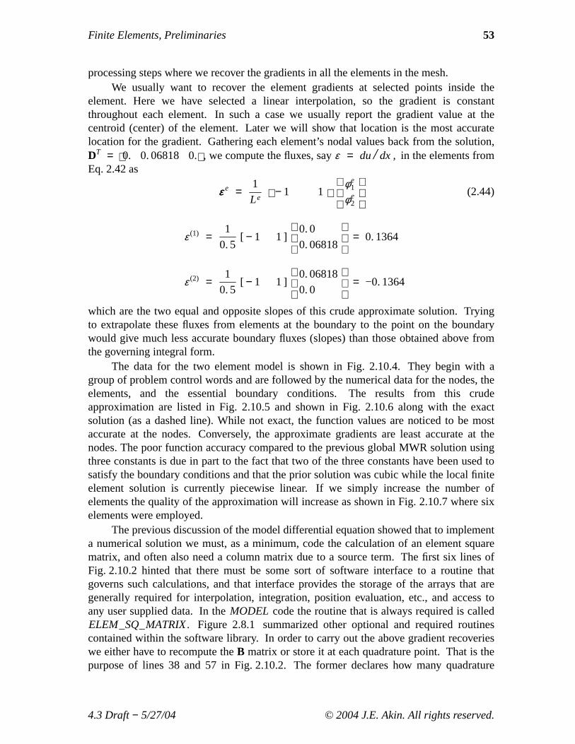
processing steps where we recover the gradients in all the elements in the mesh.We usually want to recover the element gradients at selected points inside the
element. Here we have selected a linear interpolation, so the gradient is constantthroughout each element. In such a case we usually report the gradient value at thecentroid (center) of the element. Later we will show that location is the most accuratelocation for the gradient. Gathering each element’s nodal values back from the solution,DT = 0. 0. 06818 0. , we compute the fluxes, sayε = du/ dx , in the elements fromEq. 2.42 as
(2.44)εε e =1
Le − 1 1
φ e1
φ e2
ε (1) =1
0. 5[ − 1 1 ]
0. 0
0. 06818
= 0. 1364
ε (2) =1
0. 5[ − 1 1 ]
0. 06818
0. 0
= −0. 1364
which are the two equal and opposite slopes of this crude approximate solution. Tryingto extrapolate these fluxes from elements at the boundary to the point on the boundarywould give much less accurate boundary fluxes (slopes) than those obtained above fromthe governing integral form.
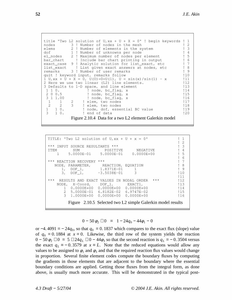
The data for the two element model is shown in Fig. 2.10.4. They begin with agroup of problem control words and are followed by the numerical data for the nodes, theelements, and the essential boundary conditions. The results from this crudeapproximation are listed in Fig. 2.10.5 and shown in Fig. 2.10.6 along with the exactsolution (as a dashed line). While not exact, the function values are noticed to be mostaccurate at the nodes. Conversely, the approximate gradients are least accurate at thenodes. The poor function accuracy compared to the previous global MWR solution usingthree constants is due in part to the fact that two of the three constants have been used tosatisfy the boundary conditions and that the prior solution was cubic while the local finiteelement solution is currently piecewise linear. If we simply increase the number ofelements the quality of the approximation will increase as shown in Fig. 2.10.7 where sixelements were employed.
The previous discussion of the model differential equation showed that to implementa numerical solution we must, as a minimum, code the calculation of an element squarematrix, and often also need a column matrix due to a source term. The first six lines ofFig. 2.10.2 hinted that there must be some sort of software interface to a routine thatgoverns such calculations, and that interface provides the storage of the arrays that aregenerally required for interpolation, integration, position evaluation, etc., and access toany user supplied data. In theMODEL code the routine that is always required is calledELEM_SQ_MATRIX. Figure 2.8.1 summarized other optional and required routinescontained within the software library. In order to carry out the above gradient recoverieswe either have to recompute theB matrix or store it at each quadrature point. That is thepurpose of lines 38 and 57 in Fig. 2.10.2. The former declares how many quadrature
4.3 Draft− 5/27/04 © 2004 J.E. Akin. All rights reserved.

54 J. E. Akin
0 0.1 0.2 0.3 0.4 0.5 0.6 0.7 0.8 0.9 10
0.01
0.02
0.03
0.04
0.05
0.06
0.07
X, Node number at 45 deg, Element number at 90 deg
Exact (dash) & FEA Solution Component_1: 2 Elements, 3 Nodes
Com
pone
nt 1
(m
ax =
0.0
6818
2, m
in =
0)
(1
)
(2
)
1
2
3
−−−min
−−−max
U’’ + U + X = 0, Two L2 elements
Figure 2.10.6 Results from exact (-) and two linear elements (solid)
0 0.1 0.2 0.3 0.4 0.5 0.6 0.7 0.8 0.9 10
0.01
0.02
0.03
0.04
0.05
0.06
0.07
X, Node number at 45 deg, Element number at 90 deg
Exact (dash) & FEA Solution Component_1: 6 Elements, 7 Nodes
Com
pone
nt 1
(m
ax =
0.0
6956
8, m
in =
0)
(1
)
(2
)
(3
)
(4
)
(5
)
(6
)
1
2
3
4
5
6
7
−−−min
−−−max
U’’ + U + X = 0. Six L2 Elements
Figure 2.10.7 Results from exact (-) and six linear elements (solid)
4.3 Draft− 5/27/04 © 2004 J.E. Akin. All rights reserved.
Finite Elements, Preliminaries 55
! ... Partial Global Access Arrays ! 1REAL(DP) :: C (LT_FREE), S (LT_FREE, LT_FREE) ! Results ! 2REAL(DP) :: PT (LT_PARM, LT_QP), WT (LT_QP) ! Quadratures ! 3REAL(DP) :: H (LT_N), DGH (N_SPACE, LT_N) ! Solution & deriv ! 4REAL(DP) :: COORD (LT_N, N_SPACE) ! Elem coordinates ! 5REAL(DP) :: XYZ (N_SPACE) ! Pt coordinates ! 6
! 7! ... Partial Notations List ! 8! COORD = SPATIAL COORDINATES OF ELEMENT’S NODES ! 9! DGH = GLOBAL DERIVATIVES SCALAR INTERPOLATION FUNCTIONS !10! H = SCALAR INTERPOLATION FUNCTIONS !11! LT_FREE = NUMBER OF DEGREES OF FREEDOM !12! LT_PARM = DIMENSION OF PARAMETRIC SPACE !13! LT_QP = NUMBER OF QUADRATURE POINTS !14! LT_N = NUMBER OF NODES PER ELEMENT !15! N_SPACE = DIMENSION OF PHYSICAL SPACE !16! PT = QUADRATURE COORDINATES !17! WT = QUADRATURE WEIGHTS !18! XYZ = PHYSICAL POINT !19
!20! .......................................................... !21! ** ELEM_SQ_MATRIX PROBLEM DEPENDENT STATEMENTS FOLLOW ** !22! .......................................................... !23! Define new array or variable types, then give statements !24! !25! APPLICATION DEPENDENT Galerkin MWR via Gauss quadratures !26! U,xx + U + X = 0, with boundary conditions like !27! U(0)=0=U(1), s o U = sin(x)/sin(1) - x or !28! U(0)=0,U’(1)=0, so U = sin(x)/cos(1) - x etc !29
!30REAL(DP) :: DL, DX_DR ! Length, Jacobian !31INTEGER :: IQ ! Loops !32
!33DL = COORD (LT_N, 1) - COORD (1, 1) ! LENGTH !34DX_DR = DL / 2. ! CONSTANT JACOBIAN !35E = 1.d0 ! CONSTANT E !36
!37CALL STORE_FLUX_POINT_COUNT ! Save LT_QP for post-process !38
!39DO IQ = 1, LT_QP ! LOOP OVER QUADRATURES !40
!41! GET INTERPOLATION FUNCTIONS, AND X-COORD !42
H = GET_H_AT_QP (IQ) !43XYZ = MATMUL (H, COORD) ! ISOPARAMETRIC !44
!45! LOCAL AND GLOBAL DERIVATIVES, B = DGH !46
DLH = GET_DLH_AT_QP (IQ) ; DGH = DLH / DX_DR !47!48
! SOURCE VECTOR WITH Q(X) = X = XYZ (1) !49C = C + H * XYZ (1) * WT (IQ) * DX_DR !50
!51! SQUARE MATRIX !52
S = S + ( MATMUL (TRANSPOSE(DGH), DGH) & !53- OUTER_PRODUCT (H, H) ) * WT (IQ) * DX_DR !54
!55! SAVE FOR FLUX AVERAGING OR POST PROCESSING, B == DGH !56
CALL STORE_FLUX_POINT_DATA (XYZ, E, DGH) ! for post-proc !57END DO ! QUADRATURE !58
! End of application dependent code !59
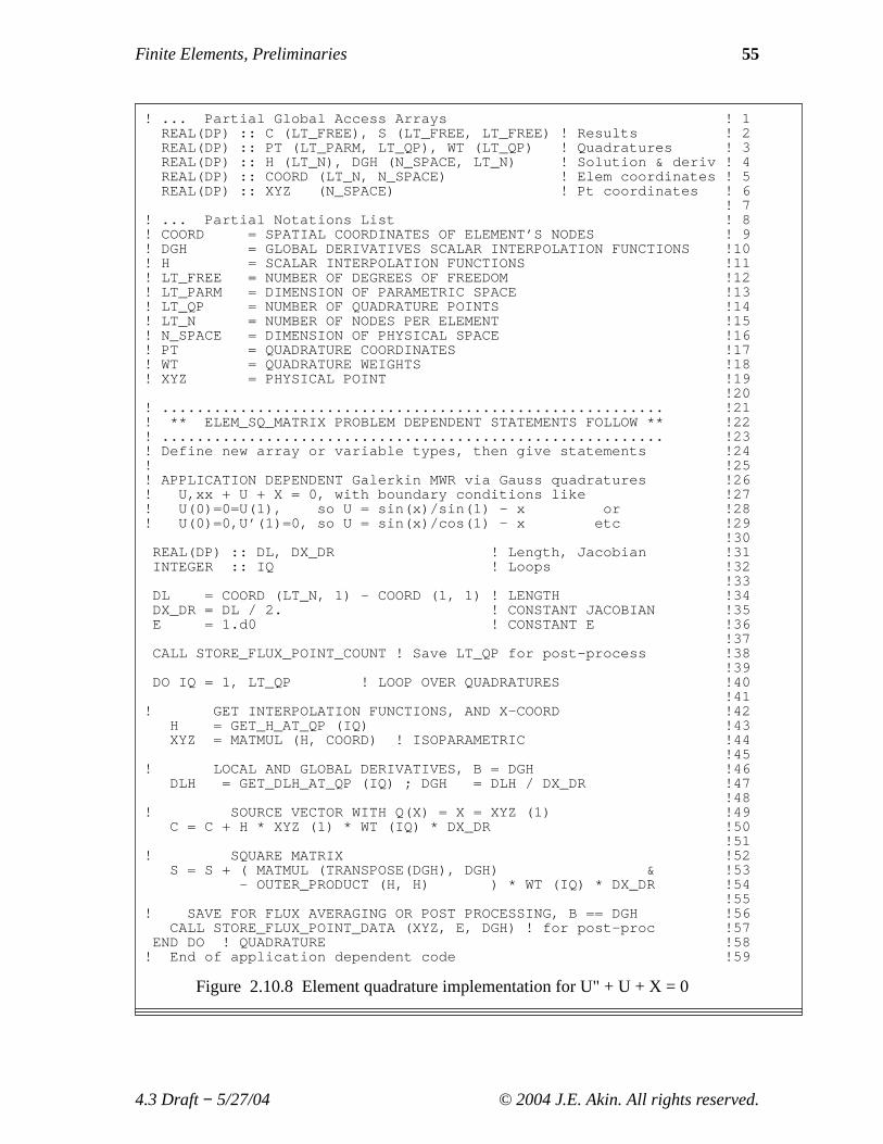
Figure 2.10.8 Element quadrature implementation for U" + U + X = 0
4.3 Draft− 5/27/04 © 2004 J.E. Akin. All rights reserved.
56 J. E. Akin
points are being used by this element type, and later line saves theB matrix and thespatial coordinate(s) of the point. (In this example, the "constitutive data" are simplyunity and are not really needed.) Thus, the post-processing loop has a similar pair ofoperations to gather those data and carry out the matrix products used above.
A typical subroutine segment for implementing any one-dimensional finite elementby numerical integration is shown in Fig. 2.10.8. The coding is valid for any line elementin the library of interpolation functions (currently linear through cubic) and the selectionof element type is set in the control data, as noted later. For a linear element a one pointquadrature rule would exactly integrate the first square matrix contribution, but a twopoint quadrature rule would be needed for the second square matrix contribution and forthe column matrix. Clearly higher degree elements require a corresponding increase inthe quadrature rule employed. The first 20 lines of that figure relate to an interface thathas not yet been described. Only lines 26 and on change with each new application class.Lines 38 and 57 are optional for later post-processing uses. Line 36 accounts for the unitcoefficient multiplying thed2u/ dx2 term in the differential equation. Usually it has someother assigned user input value.
2.11 Continuous Nodal Flux Recovery
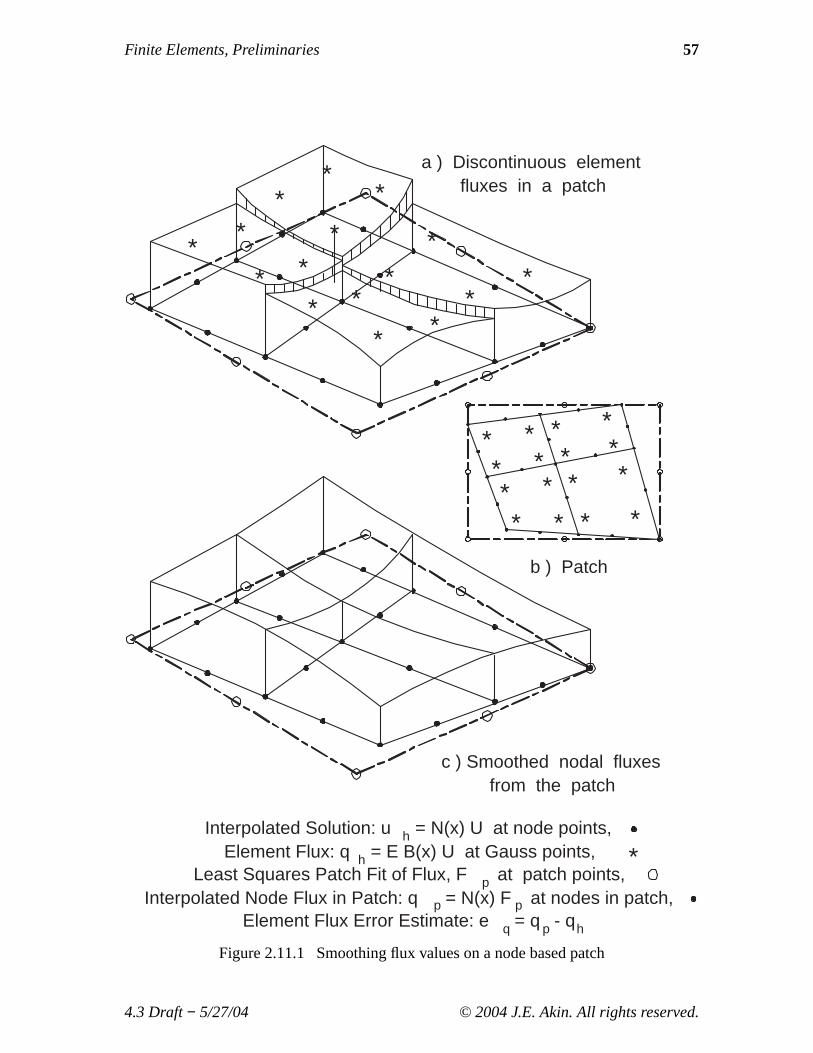
Zienkiewicz and Zhu [28, 31, 32] developed the concept of utilizing a local patchof elements, sampled at their super-convergent points, to yield a smooth set of leastsquare fit nodal gradients or fluxes. As noted earlier, the super-convergent points of anelement are the special interior locations where the gradients of the element are mostaccurate. That is, those gradient locations match those of polynomials of one or moredegrees higher. Numerous minor improvements to their original process have shown theSCP recovery process to be a practical way to get continuous nodal fluxes,σσ * . They hav edemonstrated numerically that one can generate super-convergence estimates forσσ * at anode by employing patches of elements surrounding the node. These concepts areillustrated in Fig. 2.11.1.
A local least squares fit is generated over the patch of elements in the following way.Assume a polynomial approximation of the form
(2.45)σσ * = P ( φ , η ) a
whereP denotes a polynomial (in a local parametric coordinate system selected for eachpatch) that is of the same degree and completeness that was used to approximate theoriginal solution,uh. That is,P is similar or identical to the solution interpolation arrayH. Here a represents a rectangular array that contains the nodal values of the flux.Since ˆσσ was computed using the physical derivatives ofH, σσ = EeBeφφ e. To compute theestimate forσσ * at the nodes inside the patch, we minimize the function
F (a) =n
j= 1Σ ( σσ *
j − σσ j ) 2 → min
wheren is the total number of integration points (or super-convergent points) used in theelements that define the patch andσσ j is the flux evaluated at pointx j . Substituting thetwo different interpolation functions gives
4.3 Draft− 5/27/04 © 2004 J.E. Akin. All rights reserved.
Finite Elements, Preliminaries 57
a ) Discontinuous elementfluxes in a patch
b ) Patch
c ) Smoothed nodal fluxesfrom the patch
**
**
* ***
***
*
****
*
**
***
* *
** *
* *
***
Interpolated Solution: u h = N(x) U at node points, Element Flux: q h = E B(x) U at Gauss points,
Least Squares Patch Fit of Flux, F p at patch points,Interpolated Node Flux in Patch: q p = N(x) F p at nodes in patch,
Element Flux Error Estimate: e q = q p - qh
*
Figure 2.11.1 Smoothing flux values on a node based patch
4.3 Draft− 5/27/04 © 2004 J.E. Akin. All rights reserved.

58 J. E. Akin
a ) Mesh with nodeor element
b ) Adjacent elements patch
c ) Facing elementspatch
d ) Patch of elementsat node
Figure 2.11.2 Examples of element based and node based patches
(2.46)F (a) =npe
e=1Σ
nq
j= 1Σ
P j a − Ee Be
j φφ e
2
where npe denotes the number of elements in the patch andnq is the number ofintegration points used to form ˆσσ e. That is, we are seeking a least squares fit through the
n =npe
e=1Σ
nq
j= 1Σ
data points to compute the unknown coefficients,a, which is a rectangular matrix of fluxcomponents at each node of the patch. Note that the number rows in the least squaressystem will be equal to the number of nodes defining the patch "element". Thus theabove value ofn sampling points must be equal to or greater than the number of nodes onthe patch "element" (i.e., the number of coefficients inP). The standard least squaresminimization gives the local algebraic problemS a = C where
(2.47)S =npe
e=1Σ
nq
j= 1Σ PT ( φ j , η j ) P( φ j , η j ) , C =
npe
e=1Σ
nq
j= 1Σ PT
j Ee Bej ΦΦe .
This is solved for the coefficientsa of the local patch fit. It is the cost of solving thissmall system of equations, for each patch, that we must pay in order to obtain the
4.3 Draft− 5/27/04 © 2004 J.E. Akin. All rights reserved.

Finite Elements, Preliminaries 59
continuous nodal values for the fluxes. To avoid ill-conditioning common to leastsquares, the local patch fitting parametric space (φ , η ) is mapped to enclose the patch ofelements while using a constant Jacobian for the patch. The use of the constant Jacobianis the key to the efficient conversion of the physical stress location,x j , to thecorresponding patch location,φφ j . Here the implementation actually employs a diagonalconstant Jacobian to map the patch onto the physical domain.
Zienkiewicz and Zhu have verified numerically that the derivatives estimated in thisway hav e an accuracy of at least orderO ( hp+1 ), whereh is the size of the element andpis the degree of the interpolation,N, used for the solution. There is a theorem that statesthat if theσσ * are super-convergent of orderO ( hp+α ) for α > 0, then the error estimatorwill be asymptotically exact. That is, the effectivity index should approach unity,Θ → 1.This means that we have the ability to accurately estimate the error and, thus, to get themaximum accuracy for a given number of degrees of freedom. There is not yet atheoretical explanation for the "hyperconvergent" convergence (two orders higher)reported in some of the SCP numerical studies. It may be because the least square fitdoes not go exactly through the given Barlow points. Thus, they are really samplingnearby. In Sec. 3.8 we showed that derivative sampling points for a cubic are at± 0. 577,while those for the quartic are at± 0. 707. The patch smoothing may effectively bepicking up those quartic derivative estimates and jumping to a higher degree of precision.
It is also possible to make other logical choices for selecting the elements that willconstitute a patch. Figure 2.11.2 shows two types of element based patches as well as theabove node based patch. Regardless of the types of patches selected they almost alwaysoverlap with other patches which means that the mesh nodes receive sev eral differentestimates for the continuous nodal flux value. They should be quite close to each otherbut they need to be averaged to get the final values for the continuous nodal fluxes. It ispossible to weight that averaging by the size of the contributing patch but it is simpler tojust employ a straight numerical average. The implementation of the SCP recoverymethod will be given in full detail in the next chapter after considering other errorindicator techniques.
2.12 A One-Dimensional Example Error Analysis
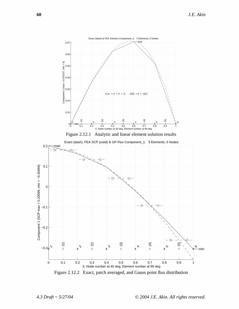
As a simple example of the process for recovering estimates of the continuous nodalflux values we will return to one of the one-dimensional models considered earlier.Figure 2.12.1 shows a five element model for a second order ODE, while thecorresponding analytic, Gauss point (o), and patch averaged flux estimates are shown inFig. 2.12.2. The piecewise linear flux estimate (solid line) in the latter figure wasobtained by using the SCP process described above. It is the relation that will be used todescribeσσ * (x) for general post-processing or for use as in the stress error estimate.
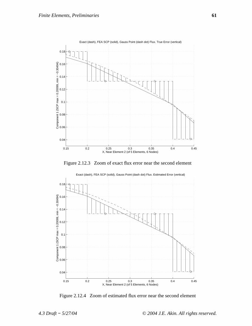
For linear interpolation elements we recall that the gradients in each element isconstant. The elements used two Gaussian quadrature points (in order to exactlyintegrate the "mass" matrix). In Figs. 2.11.3 and 4 we see a zoomed view of the variousflux representations near element number 2 (in a 5 element mesh). The horizontal dash-dot line through the quadrature point flux values represents the standard finite elementspatial distribution,Be φφ e, of the flux in that element. Again, the solid line is the spatialform of an averaged flux from a set of patches, and the dashed line is the exact flux
4.3 Draft− 5/27/04 © 2004 J.E. Akin. All rights reserved.
60 J. E. Akin
0 0.1 0.2 0.3 0.4 0.5 0.6 0.7 0.8 0.9 10
0.01
0.02
0.03
0.04
0.05
0.06
0.07
X, Node number at 45 deg, Element number at 90 deg
Exact (dash) & FEA Solution Component_1: 5 Elements, 6 Nodes
Com
pone
nt 1
(m
ax =
0.0
7075
7, m
in =
0)
(1
)
(2
)
(3
)
(4
)
(5
)
1
2
3
4
5
6
−−−min
−−−max
U,xx + U + X = 0, U(0) = 0 = U(1)
Figure 2.12.1 Analytic and linear element solution results
0 0.1 0.2 0.3 0.4 0.5 0.6 0.7 0.8 0.9 1
−0.3
−0.2
−0.1
0
0.1
0.2
X, Node number at 45 deg, Element number at 90 deg
Exact (dash), FEA SCP (solid) & GP Flux Component_1: 5 Elements, 6 Nodes
Com
pone
nt 1
(S
CP
max
= 0
.200
99, m
in =
−0.
3049
4)
(1
)
(2
)
(3
)
(4
)
(5
)
1
2
3
4
5
6
−−−min
−−−max
Figure 2.12.2 Exact, patch averaged, and Gauss point flux distribution
4.3 Draft− 5/27/04 © 2004 J.E. Akin. All rights reserved.
Finite Elements, Preliminaries 61
0.15 0.2 0.25 0.3 0.35 0.4 0.45
0.04
0.06
0.08
0.1
0.12
0.14
0.16
0.18
X, Near Element 2 (of 5 Elements, 6 Nodes)
Exact (dash), FEA SCP (solid), Gauss Point (dash dot) Flux. True Error (vertical)
Com
pone
nt 1
(S
CP
max
= 0
.200
99, m
in =
−0.
3049
4)
Figure 2.12.3 Zoom of exact flux error near the second element
0.15 0.2 0.25 0.3 0.35 0.4 0.45
0.04
0.06
0.08
0.1
0.12
0.14
0.16
0.18
X, Near Element 2 (of 5 Elements, 6 Nodes)
Exact (dash), FEA SCP (solid), Gauss Point (dash dot) Flux. Estimated Error (vertical)
Com
pone
nt 1
(S
CP
max
= 0
.200
99, m
in =
−0.
3049
4)
Figure 2.12.4 Zoom of estimated flux error near the second element
4.3 Draft− 5/27/04 © 2004 J.E. Akin. All rights reserved.
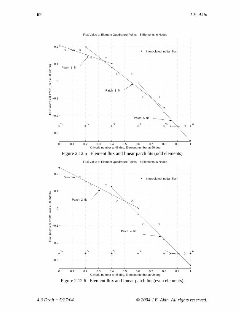
62 J. E. Akin
0 0.1 0.2 0.3 0.4 0.5 0.6 0.7 0.8 0.9 1
−0.3
−0.2
−0.1
0
0.1
0.2
X, Node number at 45 deg, Element number at 90 deg
Flux Value at Element Quadrature Points: 5 Elements, 6 Nodes
Flu
x (
max
= 0
.179
81, m
in =
−0.
2615
6)
1
2
3
4
5
6
−−−min
−−−max +
+
+
++
+
+
+
+
+
+
Patch 1 fit
Patch 3 fit
Patch 5 fit
Interpolated nodal flux
Figure 2.12.5 Element flux and linear patch fits (odd elements)
0 0.1 0.2 0.3 0.4 0.5 0.6 0.7 0.8 0.9 1
−0.3
−0.2
−0.1
0
0.1
0.2
X, Node number at 45 deg, Element number at 90 deg
Flux Value at Element Quadrature Points: 5 Elements, 6 Nodes
Flu
x (
max
= 0
.179
81, m
in =
−0.
2615
6)
1
2
3
4
5
6
−−−min
−−−max +
+
+
+
+
+
+
+
+
+
Patch 2 fit
Patch 4 fit
Interpolated nodal flux
Figure 2.12.6 Element flux and linear patch fits (even elements)
4.3 Draft− 5/27/04 © 2004 J.E. Akin. All rights reserved.
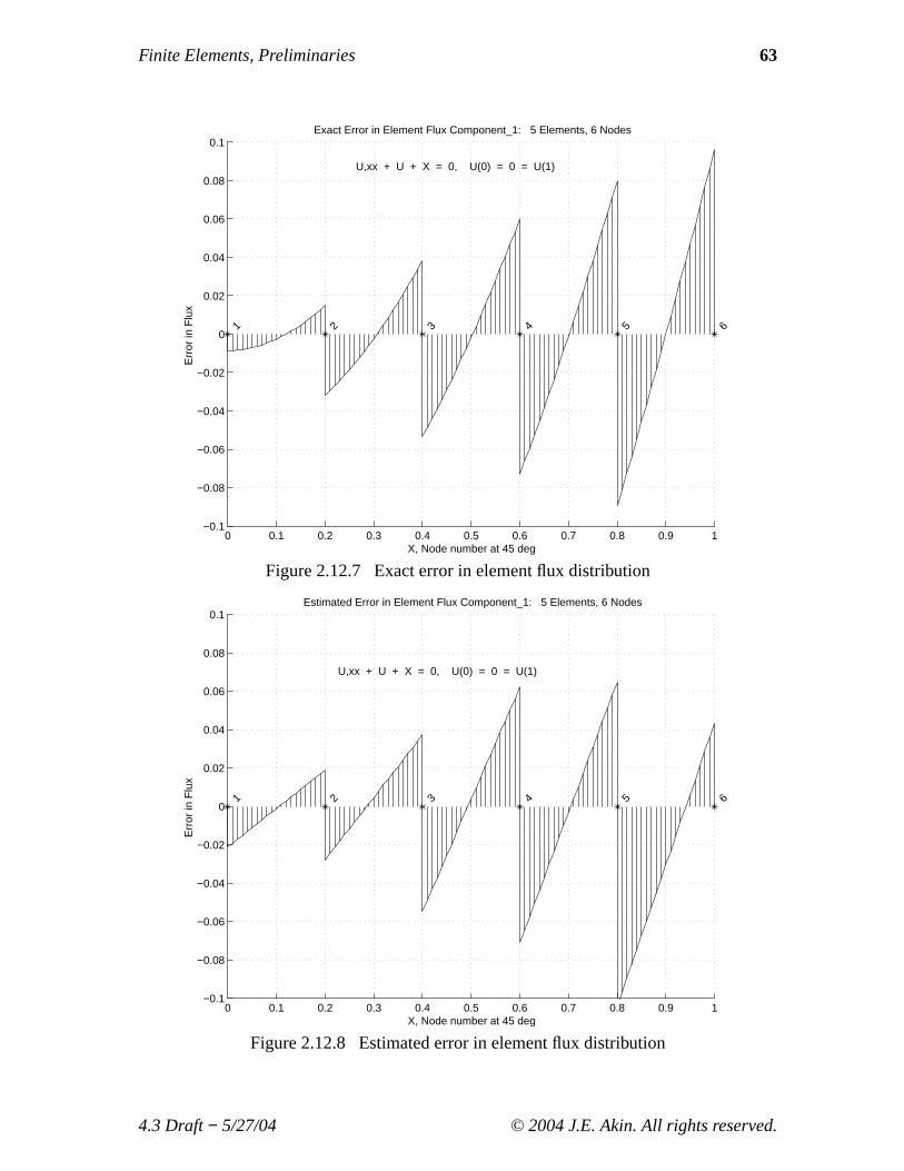
Finite Elements, Preliminaries 63
0 0.1 0.2 0.3 0.4 0.5 0.6 0.7 0.8 0.9 1−0.1
−0.08
−0.06
−0.04
−0.02
0
0.02
0.04
0.06
0.08
0.1
X, Node number at 45 deg
Exact Error in Element Flux Component_1: 5 Elements, 6 Nodes
Err
or in
Flu
x
1
2
3
4
5
6
U,xx + U + X = 0, U(0) = 0 = U(1)
Figure 2.12.7 Exact error in element flux distribution
0 0.1 0.2 0.3 0.4 0.5 0.6 0.7 0.8 0.9 1−0.1
−0.08
−0.06
−0.04
−0.02
0
0.02
0.04
0.06
0.08
0.1
X, Node number at 45 deg
Estimated Error in Element Flux Component_1: 5 Elements, 6 Nodes
Err
or in
Flu
x
1
2
3
4
5
6
U,xx + U + X = 0, U(0) = 0 = U(1)
Figure 2.12.8 Estimated error in element flux distribution
4.3 Draft− 5/27/04 © 2004 J.E. Akin. All rights reserved.
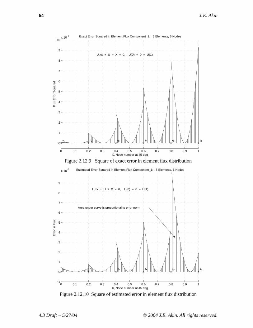
64 J. E. Akin
0 0.1 0.2 0.3 0.4 0.5 0.6 0.7 0.8 0.9 1
0
1
2
3
4
5
6
7
8
9
10x 10
−3
X, Node number at 45 deg
Exact Error Squared in Element Flux Component_1: 5 Elements, 6 Nodes
Flu
x E
rror
Squ
ared
1
2
3
4
5
6
U,xx + U + X = 0, U(0) = 0 = U(1)
Figure 2.12.9 Square of exact error in element flux distribution
0 0.1 0.2 0.3 0.4 0.5 0.6 0.7 0.8 0.9 1−1
0
1
2
3
4
5
6
7
8
9
x 10−3
X, Node number at 45 deg
Estimated Error Squared in Element Flux Component_1: 5 Elements, 6 Nodes
Err
or in
Flu
x
1
2
3
4
5
6
U,xx + U + X = 0, U(0) = 0 = U(1)
Area under curve is proportional to error norm
Figure 2.12.10 Square of estimated error in element flux distribution
4.3 Draft− 5/27/04 © 2004 J.E. Akin. All rights reserved.
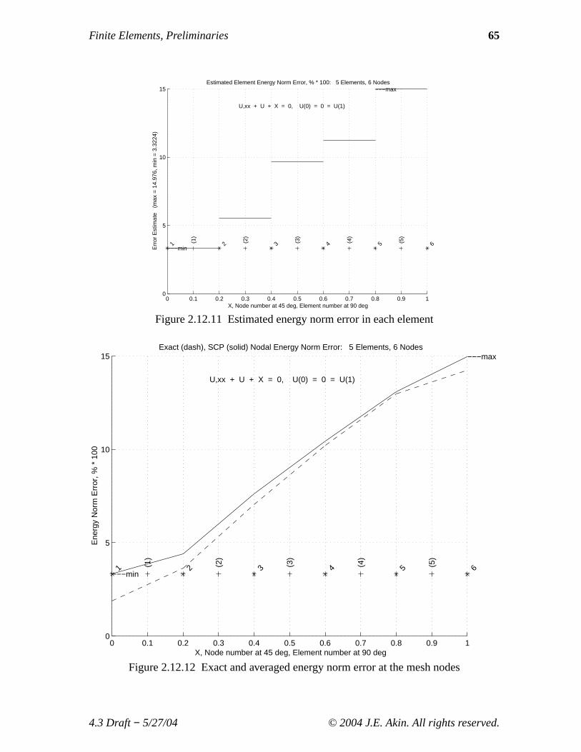
Finite Elements, Preliminaries 65
0 0.1 0.2 0.3 0.4 0.5 0.6 0.7 0.8 0.9 10
5
10
15
X, Node number at 45 deg, Element number at 90 deg
Estimated Element Energy Norm Error, % * 100: 5 Elements, 6 Nodes
Err
or E
stim
ate
(m
ax =
14.
976,
min
= 3
.322
4)
(1
)
(2
)
(3
)
(4
)
(5
)
1
2
3
4
5
6
−−−min
−−−max
U,xx + U + X = 0, U(0) = 0 = U(1)
Figure 2.12.11 Estimated energy norm error in each element
0 0.1 0.2 0.3 0.4 0.5 0.6 0.7 0.8 0.9 10
5
10
15
X, Node number at 45 deg, Element number at 90 deg
Exact (dash), SCP (solid) Nodal Energy Norm Error: 5 Elements, 6 Nodes
Ene
rgy
Nor
m E
rror
, % *
100
(1
)
(2
)
(3
)
(4
)
(5
)
1
2
3
4
5
6
−−−min
−−−max
U,xx + U + X = 0, U(0) = 0 = U(1)
Figure 2.12.12 Exact and averaged energy norm error at the mesh nodes
4.3 Draft− 5/27/04 © 2004 J.E. Akin. All rights reserved.
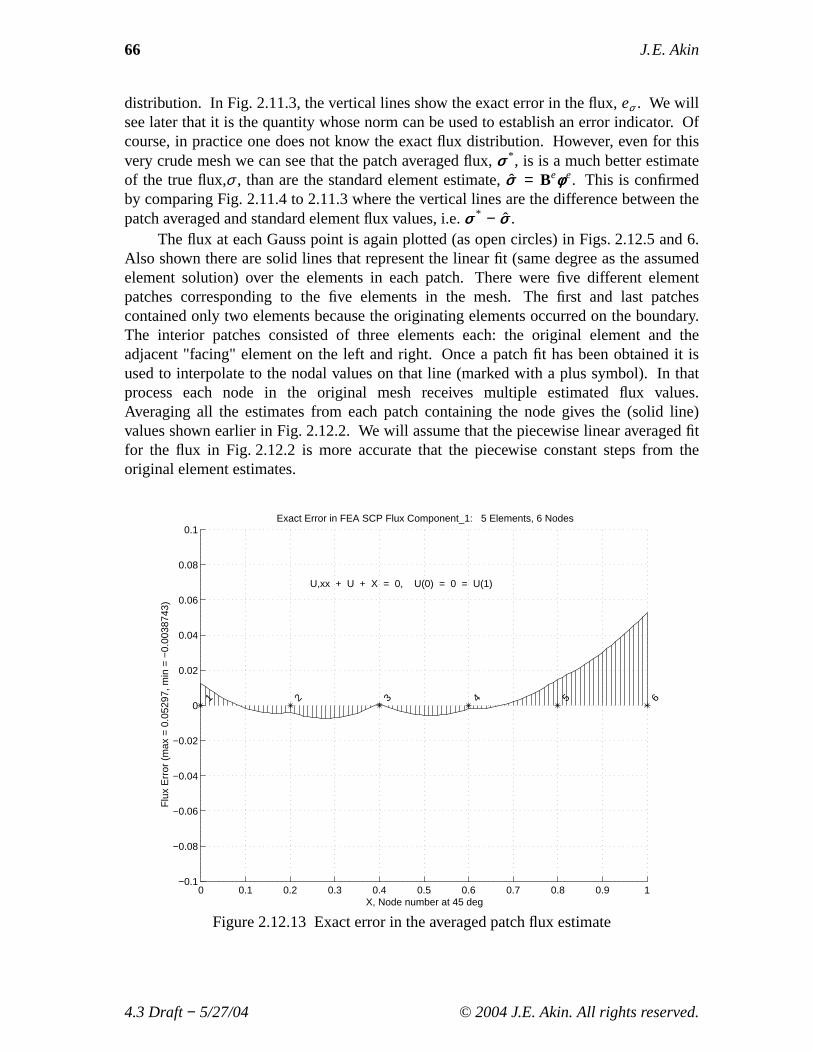
66 J. E. Akin
distribution. In Fig. 2.11.3, the vertical lines show the exact error in the flux,eσ . We willsee later that it is the quantity whose norm can be used to establish an error indicator. Ofcourse, in practice one does not know the exact flux distribution. However, even for thisvery crude mesh we can see that the patch averaged flux,σσ * , is is a much better estimateof the true flux,σ , than are the standard element estimate, ˆσσ = Beφφ e. This is confirmedby comparing Fig. 2.11.4 to 2.11.3 where the vertical lines are the difference between thepatch averaged and standard element flux values, i.e.σσ * − σσ .
The flux at each Gauss point is again plotted (as open circles) in Figs. 2.12.5 and 6.Also shown there are solid lines that represent the linear fit (same degree as the assumedelement solution) over the elements in each patch. There were five different elementpatches corresponding to the five elements in the mesh. The first and last patchescontained only two elements because the originating elements occurred on the boundary.The interior patches consisted of three elements each: the original element and theadjacent "facing" element on the left and right. Once a patch fit has been obtained it isused to interpolate to the nodal values on that line (marked with a plus symbol). In thatprocess each node in the original mesh receives multiple estimated flux values.Av eraging all the estimates from each patch containing the node gives the (solid line)values shown earlier in Fig. 2.12.2. We will assume that the piecewise linear averaged fitfor the flux in Fig. 2.12.2 is more accurate that the piecewise constant steps from theoriginal element estimates.
0 0.1 0.2 0.3 0.4 0.5 0.6 0.7 0.8 0.9 1−0.1
−0.08
−0.06
−0.04
−0.02
0
0.02
0.04
0.06
0.08
0.1
X, Node number at 45 deg
Exact Error in FEA SCP Flux Component_1: 5 Elements, 6 Nodes
Flu
x E
rror
(m
ax =
0.0
5297
, min
= −
0.00
3874
3)
1
2
3
4
5
6
U,xx + U + X = 0, U(0) = 0 = U(1)
Figure 2.12.13 Exact error in the averaged patch flux estimate
4.3 Draft− 5/27/04 © 2004 J.E. Akin. All rights reserved.
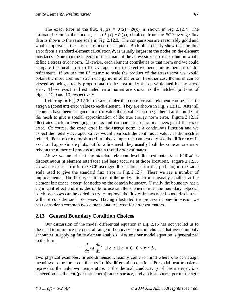
Finite Elements, Preliminaries 67
The exact error in the flux,eσ (x) ≡ σσ (x) − σσ (x), is shown in Fig. 2.12.7. Theestimated error in the flux,eσ ≈ σσ * (x) − σσ (x), obtained from the SCP average fluxdata is shown to the same scale in Fig. 2.12.8. The comparisons are reasonably good andwould improve asthe mesh is refined or adapted. Both plots clearly show that the fluxerror from a standard element calculation, ˆσσ , is usually largest at the nodes on the elementinterfaces. Note that the integral of the square of the above stress error distribution woulddefine a stress error norm. Likewise, each element contributes to that norm and we couldcompare the local error to the average error to select elements for refinement or de-refinement. If we use theEe matrix to scale the product of the stress error we wouldobtain the more common strain energy norm of the error. In either case the norm can beviewed as being directly proportional to the area under the curve defined by the stresserror. Those exact and estimated error norms are shown as the hatched portions ofFigs. 2.12.9 and 10, respectively.
Referring to Fig. 2.12.10, the area under the curve for each element can be used toassign a (constant) error value to each element. They are shown in Fig. 2.12.11. After allelements have been assigned an error value those values can be gathered at the nodes ofthe mesh to give a spatial approximation of the true energy norm error. Figure 2.12.12illustrates such an averaging process and compares it to a similar average of the exacterror. Of course, the exact error in the energy norm is a continuous function and weexpect the nodally averaged values would approach the continuous values as the mesh isrefined. For the crude mesh used in this example one can actually see the differences inexact and approximate plots, but for a fine mesh they usually look the same an one mustrely on the numerical process to obtain useful error estimates.
Above we noted that the standard element level flux estimate, ˆσσ = EeBeφφ e isdiscontinuous at element interfaces and least accurate at those locations. Figure 2.12.13shows the exact error in the SCP averaged flux estimates for this problem, to the samescale used to give the standard flux error in Fig. 2.12.7. There we see a number ofimprovements. The flux is continuous at the nodes. Its error is usually smallest at theelement interfaces, except for nodes on the domain boundary. Usually the boundary has asignificant effect and it is desirable to use smaller elements near the boundary. Specialpatch processes can be added to try to improve the flux estimates near boundaries but wewill not consider such processes. Having illustrated the process in one-dimension wenext consider a common two-dimensional test case for error estimators.
2.13 General Boundary Condition Choices
Our discussion of the model differential equation in Eq. 2.15 has not yet led us tothe need to introduce the general range of boundary condition choices that we commonlyencounter in applying finite element analysis. Assume our model equation is generalizedto the form
−d
dx(a
du
dx) + b u + c = 0, 0 < x < L .
Tw o physical examples, in one-dimension, readily come to mind where one can assignmeanings to the three coefficients in this differential equation. For axial heat transferurepresents the unknown temperature,a the thermal conductivity of the material,b aconvection coefficient (per unit length) on the surface, andc a heat source per unit length
4.3 Draft− 5/27/04 © 2004 J.E. Akin. All rights reserved.
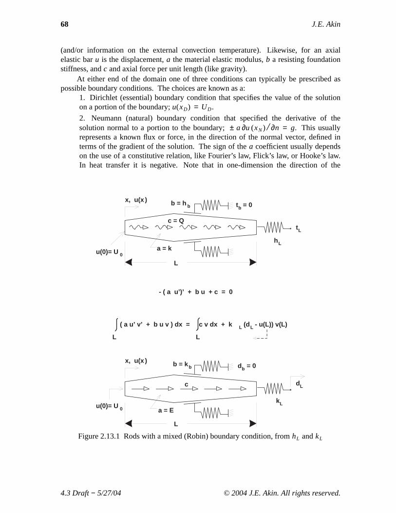
68 J. E. Akin
(and/or information on the external convection temperature). Likewise, for an axialelastic baru is the displacement,a the material elastic modulus,b a resisting foundationstiffness, andc and axial force per unit length (like gravity).
At either end of the domain one of three conditions can typically be prescribed aspossible boundary conditions. The choices are known as a:
1. Dirichlet (essential) boundary condition that specifies the value of the solutionon a portion of the boundary;u(xD) = UD.
2. Neumann (natural) boundary condition that specified the derivative of thesolution normal to a portion to the boundary;± a ∂u (xN) / ∂n = g. This usuallyrepresents a known flux or force, in the direction of the normal vector, defined interms of the gradient of the solution. The sign of thea coefficient usually dependson the use of a constitutive relation, like Fourier’s law, Flick’s law, or Hooke’s law.In heat transfer it is negative. Note that in one-dimension the direction of the
x, u(x )
L
a = ku(0)= U 0
x, u(x )
L
a = Eu(0)= U 0
c
b = k b
dL
kL
h L
tL
b = h b
c = Q
tb = 0
db = 0
( a u’ v’ + b u v ) dx = c v dx + k L (d L - u(L)) v(L)
L L
- ( a u’)’ + b u + c = 0
Figure 2.13.1 Rods with a mixed (Robin) boundary condition, fromhL andkL
4.3 Draft− 5/27/04 © 2004 J.E. Akin. All rights reserved.
Finite Elements, Preliminaries 69
outward normal reverses directions and∂ / ∂n = ± ∂ / ∂x.
3. Robin (mixed) boundary condition that specifies a linear combination of thenormal derivative and solution value on a portion of the boundary;± a ∂u(xR) / ∂n + f u(xR) = g. The mixed condition occurs often in heat transfer
as a convection boundary condition and sometimes as a linearized approximation toa radiation condition. In stress analysis it is less common and usually representsthe effect of an elastic support foundation, with settlement. The generalized mixedcondition notation here is:a ∂u(xR) / ∂n + r1 u(xR) + r2 = 0. The most commonexample of this type of boundary condition is heat convection from a surface wherethe normal flux is −kn(xR) ∂u(xR) / ∂n − h(xR) [u(xR) − u∞(xR)] = 0 so thatr1 = h andr2 = − hu∞, whereu(xR) is the unknown temperature on the convectingsurface,u∞(xR) is the known surrounding fluid temperature,h is the convectioncoefficient, andkn the thermal conductivity normal to the boundary.
In terms of the effects on the corresponding algebraic equation system a Dirichletcondition reduces the number of primary unknowns to be solved. That is, it reduces thesize of the effective algebraic system that must be solved (see the following section).However, it also introduces an unknown nodal reaction term in the RHS that canoptionally be recovered, as noted below. A Neumann condition does not change the sizeof the algebraic system; it simply adds known additional terms to the RHS. If that valueis zero then no action is required and it is then usually called a natural boundarycondition. A Robin, or mixed, condition likewise adds known additional terms to theRHS but, more importantly, it also adds a known symmetric square matrix contribution tothe LHS in the rows and columns that correspond to the Robin surface nodes (usuallyheat convection nodes). For the one-dimensional problems considered in this chapter theRobin, or mixed condition can only occur at an end point ( a single dof). For that nodenumber the value ofr1 is added to the diagonal of the system square matrix, and the valueof − r2 is added to the corresponding row on the RHS (or for the common convectioncase addhb Ab and hb Ab ub
∞, respectively for a convecting areaA at the point). Thecorresponding Robin boundary contributions in 2-D will be covered in Section 4.3.Figure 2.13.1 illustrates a thermal (top) and stress problem, in 1-D, with a Dirichletcondition on the left (x = 0) end and a Robin condition on the right end (x = L).
2.14 General Matrix Partitions
The above small example has lead to the most general form of the algebraic systemthat results from satisfying the required integral form: a singular matrix system with moreunknowns that equations. That is because we chose to apply the essential boundaryconditions last and there is not a unique solution until that is done. The algebraic systemcan be written in a general matrix form that more clearly defines what must be done toreduce the system to a solvable form by utilizing essential boundary condition values.Note that the system degrees of freedom,D, and the full equations could always be re-arranged in the following partitioned matrix form
(2.48)
Suu
Sk u
Su k
Sk k
Du
Dk
=
Cu
Ck + Pk
4.3 Draft− 5/27/04 © 2004 J.E. Akin. All rights reserved.
70 J. E. Akin
where Du represents the unknown nodal parameters, andDk represents the knownessential boundary values of the other parameters. The sub-matricesSuu and Sk k aresquare, whereasSu k andSk u are rectangular, in general. In a finite element formulationall of the coefficients in theS and C matrices are known. ThePk term represents thatthere are usually unknown generalized reactions associated with essential boundaryconditions. This means that in general after the essential boundary conditions (Dk) areprescribed the remaining unknowns areDu and Pk. Then the net number of unknownscorresponds to the number of equations, but they must be re-arranged before all theremaining unknowns can be computed.
Here, for simplicity, it has been assumed that the equations have been numbered in amanner that places the prescribed parameters (essential boundary conditions) at the endof the system equations. The above matrix relations can be rewritten as
Suu Du + Su k Dk = Cu
Sk u Du + Sk k Dk = Ck + Pk
so that the unknown nodal parameters are obtained by inverting the non-singular squarematrixSuu in the top partitioned rows. That is,
Du = S−1uu ( Cu − Su k Dk ) .
Most books on numerical analysis assume that you have reduced the system to the non-singular form given above where the essential conditions,Du, hav e already been movedto the right hand side. Many authors use examples with null conditions (Dk is zero) sothe solution is the simplest form,Du = S−1
uu Cu. If desired, the values of the necessaryreactions,Pk, can now be determined from
Pk = Sk u Du + Sk k Dk − Ck
In nonlinear and time dependent applications the reactions can be found from similarcalculations. In most applications the reaction data have physical meanings that areimportant in their own right, or useful in validation the solution. However, this part of thecalculations is optional. If one formulates a finite element model that satisfies theessential boundary conditions in advance then the second row of the partitioned systemSmatrix is usually not generated and one can not recover reaction data.
2.15 Elliptic Boundary Value Problems
2.15.1 One-Dimensional EquationsSince the previous model equation had an exact solution that was trigonometric our
approximation with polynomials could never giv e an exact solution (but could reach aspecified level of accuracy). Here we will consider an example where the finite elementsolution can be nodally exact and possibly exact everywhere. The following one-dimensional (ns = 1) model problem which will serve as an analytical example:
(2.49)kd2φdx2
+ Q = 0
on the closed domain,x ∈ ] 0, L [ , and is subjected to the boundary conditions
4.3 Draft− 5/27/04 © 2004 J.E. Akin. All rights reserved.
Finite Elements, Preliminaries 71
φ ( L ) = φ L , and k dφ / dx (0) = q0. Note that we have dropped the second term in theprevious ODE. The corresponding governing integral statement to be used for the finiteelement model is obtained from theGalerkin weighted residual method, followed byintegration by parts and is very similar to the first example. In this case, it states that thefunction,φ , which satisfies the essential condition,φ ( L ) = φ L , and satisfies
(2.50)I = ∫L
0
k (dφ / dx)2 − φ Q
dx + q0 φ ( 0 ) − qL φ ( L ) = 0 ,
also satisfies the new ODE. A typical element contribution is:
(2.51)I e = DeTSe De − DeT
Ce ,
where
Se ≡Le∫ ke dHeT
dx
dHe
dxdx =
Le∫ BeT
ke Be dx , Ce ≡Le∫ Qe HeT
dx .
The system of algebraic equations from the weak form isS D = C where
S =ne
e = 1Σ ββ eT
Se ββ e , C =ne
e = 1Σ ββ eT
Ce +nb
b=1Σ ββ bT
Cb ,
and where, as before,ββ denotes a set of symbolic bookkeeping operations. If we select alinear element with the interpolation relations given previously the element matrices are:
Se =ke
Le
1
−1
−1
1
, Ce =
Le∫
Qe
Le
(x2e − x)
(x − x1e)
d x .
Assuming thatQ = Q0 , a constant, this simplifies toCeT= 1 1 Q0 Le / 2. The exact
solution of the original problem for constantQ = Q0 is
(2.52)k φ (x) = k φ L + q(x − L) + Q0 ( L2 − x2 ) / 2 .
Since forQ0 ≠ 0 the exact value is quadratic and the selected element is linear, our finiteelement model can give only an approximate solution. However, for the homogeneousproblemQ0 = 0 , the model can (and does) give an exact solution. To compare a finiteelement spatial approximation with the exact one, select a two element model. Let theelements be of equal length,Le = L / 2. Then the element matrices are the same for bothelements. The assembly process (including boundary effects) yields,S D = C :
2k
L
1
−1
0
−1
(1 + 1)
−1
0
−1
1
φ1
φ2
φ3
=Q0 L
4
1
(1 + 1)
1
−
q0
0
−qL
.
However, these equations do not yet satisfy the essential boundary condition ofφ (L) = φ3 = φ L . That is,S is singular and can not be inverted. After applying thisessential boundary condition, the reduced equations are
2k
L
1
−1
− 1
2
φ1
φ2
=Q2 L
4
1
2
−
q
0
+2ktL
L
0
1
,
or Sr Dr = Cr . Inv ertingSr and solving forDr = S−1r Cr yields
4.3 Draft− 5/27/04 © 2004 J.E. Akin. All rights reserved.
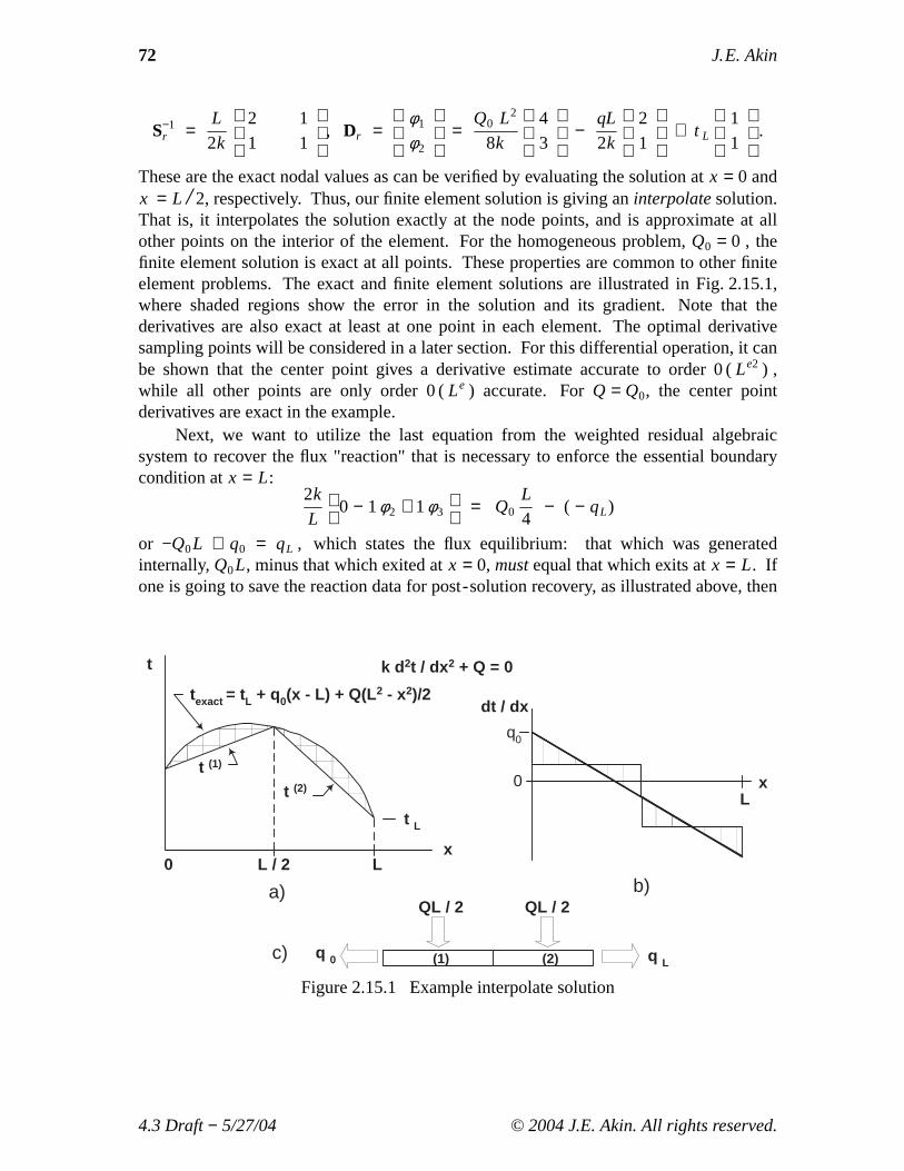
72 J. E. Akin
S−1r =
L
2k
2
1
1
1
, Dr =
φ1
φ2
=Q0 L2
8k
4
3
−qL
2k
2
1
+ t L
1
1
.
These are the exact nodal values as can be verified by evaluating the solution atx = 0 andx = L / 2, respectively. Thus, our finite element solution is giving aninterpolatesolution.That is, it interpolates the solution exactly at the node points, and is approximate at allother points on the interior of the element. For the homogeneous problem,Q0 = 0 , thefinite element solution is exact at all points. These properties are common to other finiteelement problems. The exact and finite element solutions are illustrated in Fig. 2.15.1,where shaded regions show the error in the solution and its gradient. Note that thederivatives are also exact at least at one point in each element. The optimal derivativesampling points will be considered in a later section. For this differential operation, it canbe shown that the center point gives a derivative estimate accurate to order 0 (Le2 ) ,while all other points are only order 0 (Le ) accurate. ForQ = Q0, the center pointderivatives are exact in the example.
Next, we want to utilize the last equation from the weighted residual algebraicsystem to recover the flux "reaction" that is necessary to enforce the essential boundarycondition atx = L:
2k
L
0 − 1φ2 + 1φ3
= Q0L
4− ( − qL)
or −Q0L + q0 = qL , which states the flux equilibrium: that which was generatedinternally,Q0L, minus that which exited atx = 0, mustequal that which exits atx = L. Ifone is going to save the reaction data for post-solution recovery, as illustrated above, then
k d 2t / dx 2 + Q = 0
x
t
texact = tL + q0(x - L) + Q(L 2 - x2)/2
t (1)
t (2)
0 L / 2 L
t L
dt / dx
x
0L
q0
QL / 2
q Lq 0
QL / 2
(1) (2)
a) b)
c)
Figure 2.15.1 Example interpolate solution
4.3 Draft− 5/27/04 © 2004 J.E. Akin. All rights reserved.
Finite Elements, Preliminaries 73
one could use programs likeSYSTEM_ROW_SAVEandGET_REACTIONSto store andlater recover the associated rows of the square matrix. It is not necessary to save thesedata when they are first generated since they can clearly be recomputed in a post-processing segment if desired. In the later examples we will invoke functions to savethese data as they are created.
2.15.2 Two-Dimensional EquationsAs an example of the utilization of Galerkin’s method in higher dimensions,
consider the following model transient linear operator:
(2.53)L(u) =∂
∂x
kx∂u
∂x
+∂
∂y
ky∂u
∂y
− Q − ζ∂u
∂t= 0 .
We get the weak form by multiplying by a test function,w(x), and setting the integral tozero. The last two terms are simply
IQ = ∫ΩQ w dΩ , Iζ = ∫Ω
ζ w∂u
∂td Ω .
Our main interest is with the first two terms
I k =Ω∫
w∂
∂x
kx∂u
∂x
+ w∂
∂y
ky∂u
∂y
d Ω
which involve the second order partial derivatives. We can remove them by invokingGreen’s theorem
Ω∫
∂Ψ∂x
−∂γ∂y
d Ω =Γ∫
γ dx + Ψ dy
where we defineΨ = w kx ∂u/ ∂x , and γ = −w ky ∂u/ ∂y . We note that an alternateform of I k is
I k =Ω∫
∂∂x
w kx∂u
∂x
+∂
∂y
w ky∂u
∂y
d Ω
−Ω∫
∂w
∂xkx
∂u
∂x+
∂w
∂yky
∂u
∂y
d Ω .
The first term is re-written by Green’s theorem
I k =Γ∫
−
w ky∂u
∂y
dx +
w kx∂u
∂x
dy
−Ω∫
kx∂w
∂x
∂u
∂x+ ky
∂w
∂y
∂u
∂y
d Ω .
For a contour integral with a unit normal vector,n, with components [nx ny ], we notethe geometric relationships are that (see Fig. 2.15.2) −dx = dsCos θ y = ds ny , and that
4.3 Draft− 5/27/04 © 2004 J.E. Akin. All rights reserved.
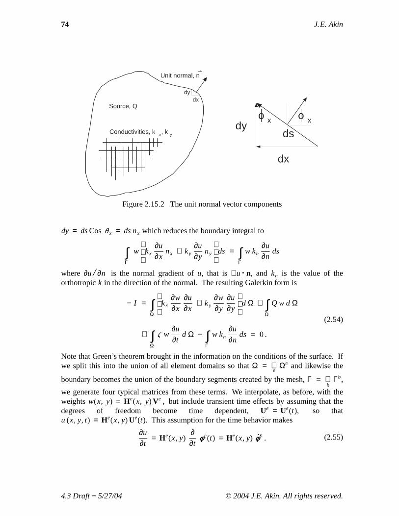
74 J. E. Akin
Source, Q
Unit normal, n
Conductivities, k x, k y
dydx
dx
dyds
o x o x
Figure 2.15.2 The unit normal vector components
dy = dsCos θ x = ds nx which reduces the boundary integral to
Γ∫ w
kx∂u
∂xnx + ky
∂u
∂yny
ds =Γ∫ w kn
∂u
∂nds
where ∂u / ∂n is the normal gradient ofu, that is ∇u.n, and kn is the value of theorthotropick in the direction of the normal. The resulting Galerkin form is
(2.54)
− I =Ω∫
kx∂w
∂x
∂u
∂x+ ky
∂w
∂y
∂u
∂y
d Ω +Ω∫ Q w dΩ
+Ω∫ ζ w
∂u
∂td Ω −
Γ∫ w kn
∂u
∂nds = 0 .
Note that Green’s theorem brought in the information on the conditions of the surface. Ifwe split this into the union of all element domains so thatΩ =
e∪ Ωe and likewise the
boundary becomes the union of the boundary segments created by the mesh,Γ =b∪ Γb,
we generate four typical matrices from these terms. We interpolate, as before, with theweightsw(x, y) = He(x, y) Ve , but include transient time effects by assuming that thedegrees of freedom become time dependent,Ue = Ue(t), so thatu (x, y, t) = He(x, y) Ue(t). This assumption for the time behavior makes
(2.55)∂u
∂t= He(x, y)
∂∂t
φφ e(t) = He(x, y) φφ e .
4.3 Draft− 5/27/04 © 2004 J.E. Akin. All rights reserved.
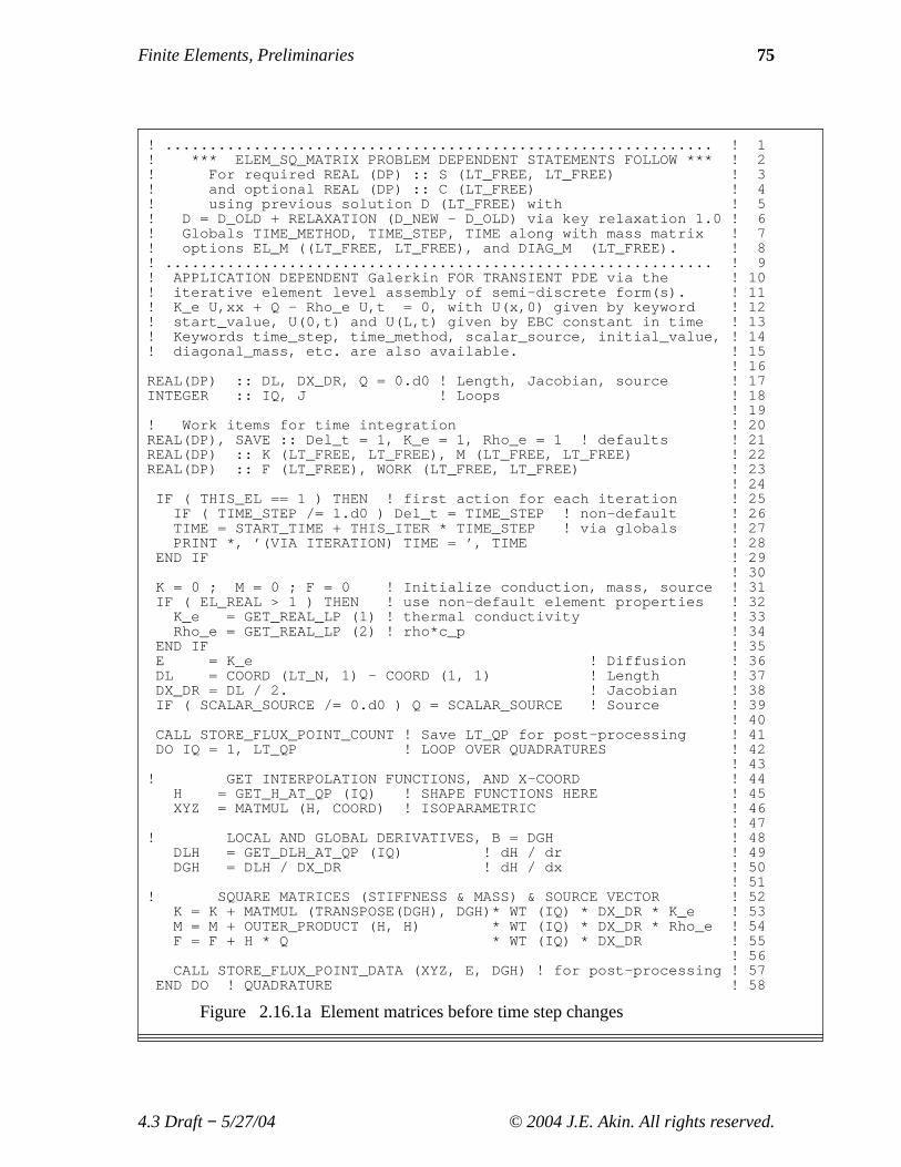
Finite Elements, Preliminaries 75
! .............................................................. ! 1! *** ELEM_SQ_MATRIX PROBLEM DEPENDENT STATEMENTS FOLLOW *** ! 2! For required REAL (DP) :: S (LT_FREE, LT_FREE) ! 3! and optional REAL (DP) :: C (LT_FREE) ! 4! using previous solution D (LT_FREE) with ! 5! D = D_OLD + RELAXATION (D_NEW - D_OLD) via key relaxation 1.0 ! 6! Globals TIME_METHOD, TIME_STEP, TIME along with mass matrix ! 7! options EL_M ((LT_FREE, LT_FREE), and DIAG_M (LT_FREE). ! 8! .............................................................. ! 9! APPLICATION DEPENDENT Galerkin FOR TRANSIENT PDE via the ! 10! iterative element level assembly of semi-discrete form(s). ! 11! K_e U,xx + Q - Rho_e U,t = 0, with U(x,0) given by keyword ! 12! start_value, U(0,t) and U(L,t) given by EBC constant in time ! 13! Keywords time_step, time_method, scalar_source, initial_value, ! 14! diagonal_mass, etc. are also available. ! 15
! 16REAL(DP) :: DL, DX_DR, Q = 0.d0 ! Length, Jacobian, source ! 17INTEGER :: IQ, J ! Loops ! 18
! 19! Work items for time integration ! 20REAL(DP), SAVE :: Del_t = 1, K_e = 1, Rho_e = 1 ! defaults ! 21REAL(DP) :: K (LT_FREE, LT_FREE), M (LT_FREE, LT_FREE) ! 22REAL(DP) :: F (LT_FREE), WORK (LT_FREE, LT_FREE) ! 23
! 24IF ( THIS_EL == 1 ) THEN ! first action for each iteration ! 25
IF ( TIME_STEP /= 1.d0 ) Del_t = TIME_STEP ! non-default ! 26TIME = START_TIME + THIS_ITER * TIME_STEP ! via globals ! 27PRINT *, ’(VIA ITERATION) TIME = ’, TIME ! 28
END IF ! 29! 30
K = 0 ; M = 0 ; F = 0 ! Initialize conduction, mass, source ! 31IF ( EL_REAL > 1 ) THEN ! use non-default element properties ! 32
K_e = GET_REAL_LP (1) ! thermal conductivity ! 33Rho_e = GET_REAL_LP (2) ! rho*c_p ! 34
END IF ! 35E = K_e ! Diffusion ! 36DL = COORD (LT_N, 1) - COORD (1, 1) ! Length ! 37DX_DR = DL / 2. ! Jacobian ! 38IF ( SCALAR_SOURCE /= 0.d0 ) Q = SCALAR_SOURCE ! Source ! 39
! 40CALL STORE_FLUX_POINT_COUNT ! Save LT_QP for post-processing ! 41DO IQ = 1, LT_QP ! LOOP OVER QUADRATURES ! 42
! 43! GET INTERPOLATION FUNCTIONS, AND X-COORD ! 44
H = GET_H_AT_QP (IQ) ! SHAPE FUNCTIONS HERE ! 45XYZ = MATMUL (H, COORD) ! ISOPARAMETRIC ! 46
! 47! LOCAL AND GLOBAL DERIVATIVES, B = DGH ! 48
DLH = GET_DLH_AT_QP (IQ) ! dH / dr ! 49DGH = DLH / DX_DR ! dH / dx ! 50
! 51! SQUARE MATRICES (STIFFNESS & MASS) & SOURCE VECTOR ! 52
K = K + MATMUL (TRANSPOSE(DGH), DGH)* WT (IQ) * DX_DR * K_e ! 53M = M + OUTER_PRODUCT (H, H) * WT (IQ) * DX_DR * Rho_e ! 54F = F + H * Q * WT (IQ) * DX_DR ! 55
! 56CALL STORE_FLUX_POINT_DATA (XYZ, E, DGH) ! for post-processing ! 57
END DO ! QUADRATURE ! 58
Figure 2.16.1a Element matrices before time step changes
4.3 Draft− 5/27/04 © 2004 J.E. Akin. All rights reserved.
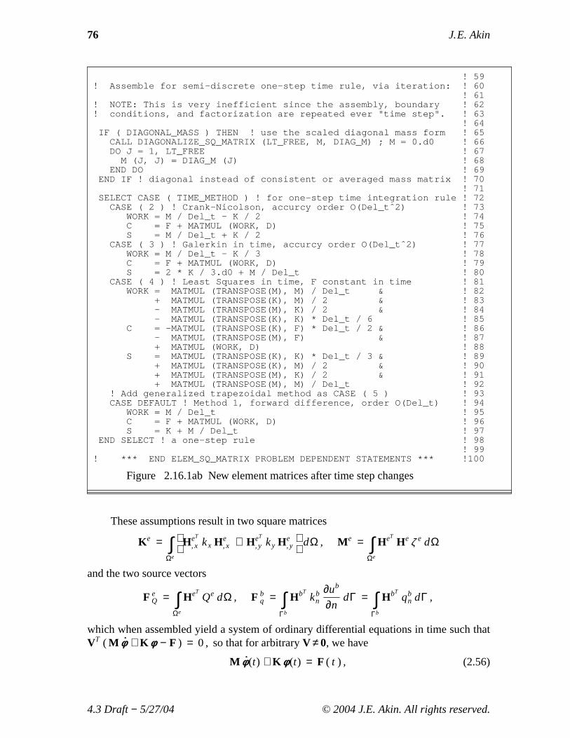
76 J. E. Akin
! 59! Assemble for semi-discrete one-step time rule, via iteration: ! 60
! 61! NOTE: This is very inefficient since the assembly, boundary ! 62! conditions, and factorization are repeated ever "time step". ! 63
! 64IF ( DIAGONAL_MASS ) THEN ! use the scaled diagonal mass form ! 65
CALL DIAGONALIZE_SQ_MATRIX (LT_FREE, M, DIAG_M) ; M = 0.d0 ! 66DO J = 1, LT_FREE ! 67
M (J, J) = DIAG_M (J) ! 68END DO ! 69
END IF ! diagonal instead of consistent or averaged mass matrix ! 70! 71
SELECT CASE ( TIME_METHOD ) ! for one-step time integration rule ! 72CASE ( 2 ) ! Crank-Nicolson, accurcy order O(Del_tˆ2) ! 73
WORK = M / Del_t - K / 2 ! 74C = F + MATMUL (WORK, D) ! 75S = M / Del_t + K / 2 ! 76
CASE ( 3 ) ! Galerkin in time, accurcy order O(Del_tˆ2) ! 77WORK = M / Del_t - K / 3 ! 78C = F + MATMUL (WORK, D) ! 79S = 2 * K / 3.d0 + M / Del_t ! 80
CASE ( 4 ) ! Least Squares in time, F constant in time ! 81WORK = MATMUL (TRANSPOSE(M), M) / Del_t & ! 82
+ MATMUL (TRANSPOSE(K), M) / 2 & ! 83- MATMUL (TRANSPOSE(M), K) / 2 & ! 84- MATMUL (TRANSPOSE(K), K) * Del_t / 6 ! 85
C = -MATMUL (TRANSPOSE(K), F) * Del_t / 2 & ! 86- MATMUL (TRANSPOSE(M), F) & ! 87+ MATMUL (WORK, D) ! 88
S = MATMUL (TRANSPOSE(K), K) * Del_t / 3 & ! 89+ MATMUL (TRANSPOSE(K), M) / 2 & ! 90+ MATMUL (TRANSPOSE(M), K) / 2 & ! 91+ MATMUL (TRANSPOSE(M), M) / Del_t ! 92
! Add generalized trapezoidal method as CASE ( 5 ) ! 93CASE DEFAULT ! Method 1, forward difference, order O(Del_t) ! 94
WORK = M / Del_t ! 95C = F + MATMUL (WORK, D) ! 96S = K + M / Del_t ! 97
END SELECT ! a one-step rule ! 98! 99
! *** END ELEM_SQ_MATRIX PROBLEM DEPENDENT STATEMENTS *** !100
Figure 2.16.1ab New element matrices after time step changes
These assumptions result in two square matrices
K e =Ωe
∫ HeT
, x kx He, x + HeT
, y ky He, y
dΩ , M e =Ωe
∫ HeTHe ζ e dΩ
and the two source vectors
F eQ =
Ωe
∫ HeTQe dΩ , F b
q =Γb
∫ HbTkb
n
∂ub
∂ndΓ =
Γb
∫ HbTqb
n dΓ ,
which when assembled yield a system of ordinary differential equations in time such thatVT ( M φφ + K φφ − F ) = 0 , so that for arbitraryV ≠ 0, we hav e
(2.56)M φφ (t) + K φφ (t) = F ( t ) ,
4.3 Draft− 5/27/04 © 2004 J.E. Akin. All rights reserved.
Finite Elements, Preliminaries 77
which is an initial value problem to be solved from the initial condition state atφφ (x, y, t = 0). Here we will note thatM e and M are usually called theelementandsystem mass(or capacity) matrices, respectively. By making assumptions about how toapproximate the time dependent vectorφφ (t) this system can be rearranged to yield alinear systemSφφ (t) = C(t) to be solved at each time step for the current value ofφφ (t).For the steady state case,∂ / ∂t = 0, this reduces to the system of algebraic equationsSφφ = C considered earlier. The same procedure is easily carried out in threedimensions. MatrixK e changes by having a third term involvingz and forFb
q we thinkof dΓ as a surface area instead of a line segment.
We also note in passing that in addition to using classical finite differences in timethere are two other choices for methods to treat time dependence. One is to do aseparation of variables and also interpolate the element behavior over one or more timesteps withu (x, y, t) = He(x, y) he(t) φφ e. [30] That allows one to carry out weightedresidual methods in time also. These first two choices are usually referred to as "semi-discrete" methods for time integration. Another approach is to carry out a full space-timeinterpolation withu (x, y, t) = He(x, y, t) φφ e [6, 7] and include three-dimensional spacevia four-dimensional elements [26]. The 4-D element solutions have very large memoryrequirements (by todays standards), and are usually restricted to a time slab (a constanttime step) which simplifies the 4-D elements and the associated 4-D mesh generation.Like the above example, most 4-D models begin with the classical mechanics laws in 3-Dspace and then interpolate through time also. It is also possible to begin the formulationusing relativity physics laws in a 4-D space-time and to form the 4-D elementstherein [16]. Such an approach is not required unless the velocities involved are not smallrelative to the speed of light.
If we had also included a second time derivative term, we could then see byinspection that it would simply introduce another mass matrix (with a differentcoefficient) times the second time derivative of the nodal degrees of freedom. This wouldthen represent thewave equationwhose solution in time could be accomplished bytechniques to be presented later. If the time derivative terms are not present, and if theterm c u is included in the PDE and if the coefficientc is an unknown global constant,then this reduces to aneigen-problem.That is, we wish to determine a set ofeigenvalues,ci , and a corresponding set ofeigenvectors,or mode shapes.
2.16 Initial Value ProblemsMany applications, like Eq. 2.53, involve the first partial derivative with respect to
time and get converted through the finite element process to a matrix system of ordinarydifferential equations in time, like Eq. 2.56. These are known as initial value problems,or parabolic problems, and require the additional description of the spatial value ofφφ atthe starting time (known as the initial condition). There are hundreds of ways tonumerically integrate these matrices in time. One has to be concerned about the relativecosts (storage and operation counts), stability, and accuracy of the chosen method. Thesetopics are covered in many books on numerical methods and we will not go into themhere. Instead we will simply give some insight to a few approaches.
If one assumes that Eq. 2.56 is valid at an element level for timets one could write
4.3 Draft− 5/27/04 © 2004 J.E. Akin. All rights reserved.
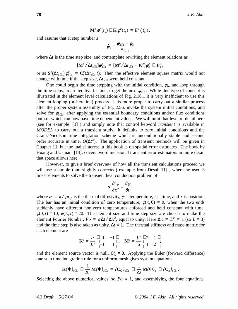
78 J. E. Akin
M e φφ e(ts) + K φφ e(ts) = Fe ( ts ) ,
and assume that at step numbers
φφ s =φφ s+1 − φφ s
∆ts+1
where∆t is the time step size, and contemplate rewriting the element relations as
[M e / ∆ts+1]φφes+1 = [M e / ∆ts+1 − K e]φφ e
s + Fes ,
or asSe(∆ts+1) φφ es+1 = Ce
s(∆ts+1,t). Then the effective element square matrix would notchange with time if the step size,∆ts+1 were held constant.
One could begin the time stepping with the initial condition,φφ0, and loop throughthe time steps, in an iterative fashion, to get the nextφφ s+1. While this type of concept isillustrated in the element level calculations of Fig. 2.16.1 it is very inefficient to use thiselement looping (or iteration) process. It is more proper to carry out a similar processafter the proper system assembly of Eq. 2.56, invoke the system initial conditions, andsolve for φφ s+1, after applying the essential boundary conditions and/or flux conditionsboth of which can now hav e time dependent values. We will omit that level of detail here(see for example [3] ) and simply note that control ketwordtransient is available inMODEL to carry out a transient study. It defaults to zero initial conditions and theCrank-Nicolson time integration scheme which is unconditionally stable and secondorder accurate in time,O(∆t2). The application of transient methods will be given inChapter 11, but the main interest in this book is on spatial error estimates. The book byHuang and Usmani [13], covers two-dimensional transient error estimators in more detailthat space allows here.
However, to giv e a brief overview of how all the transient calculations proceed wewill use a simple (and slightly corrected) example from Desai [11] , where he used 3linear elements to solve the transient heat conduction problem of
α∂2φ∂x2
=∂φ∂t
,
whereα = k / ρcp is the thermal diffusivity,φ is temperature,t is time, andx is position.The bar has an initial condition of zero temperature,φ (x, 0) = 0, when the two endssuddenly have different non-zero temperatures enforced and held constant with time,φ (0, t) = 10, φ (L, t) = 20. The element size and time step size are chosen to make theelement Fourier Number,Fo = α ∆t / ∆x2, equal to unity. Here∆x = Le = 1 (soL = 3)and the time step is also taken as unity,∆t = 1. The thermal stiffness and mass matrix foreach element are
K e =αLe
1
−1
−1
1
, M e =
Le
6
2
1
1
2
,
and the element source vector is null,CeQ = 00. Applying the Euler (forward difference)
one step time integration rule for a uniform mesh gives system equations
K ΦΦs+1 +1
∆tM ΦΦs+1 = CQs+1 +
1
∆tM ΦΦs + Cqs+1 .
Selecting the above numerical values, soFo = 1, and assemblying the four equations,
4.3 Draft− 5/27/04 © 2004 J.E. Akin. All rights reserved.
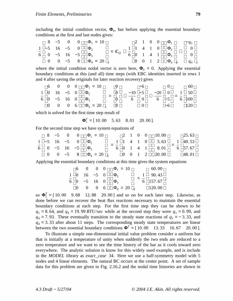
Finite Elements, Preliminaries 79
including the initial condition vector,ΦΦ0, but before applying the essential boundaryconditions at the first and last nodes gives:
1
6
8
−5
0
0
−5
16
−5
0
0
−5
16
−5
0
0
−5
8
Φ1 = 10
Φ2
Φ3
Φ4 = 20
1
= CQ +1
6
2
1
0
0
1
4
1
0
0
1
4
1
0
0
1
2
Φ1
Φ2
Φ3
Φ4
0
+
−q1
0
0
q4
1
where the initial condition nodal vector is zero here,ΦΦ0 = 0. Applying the essentialboundary conditions at this (and all) time steps (with EBC identities inserted in rows 1and 4 after saving the originals for later reaction recovery) gives
1
6
6
0
0
0
0
16
−5
0
0
−5
16
0
0
0
0
6
Φ1 = 10
Φ2
Φ3
Φ4 = 20
1
=
0
0
0
0
+−10
6
−6
−5
0
0
+−20
6
0
0
−5
−6
=1
6
60
50
100
120
which is solved for the first time step result of
ΦΦT1 = [ 10. 00 5. 63 8. 01 20. 00 ].
For the second time step we have system equations of
1
6
8
−5
0
0
−5
16
−5
0
0
−5
16
−5
0
0
−5
8
Φ1 = 10
Φ2
Φ3
Φ4 = 20
2
=1
6
2
1
0
0
1
4
1
0
0
1
4
1
0
0
1
2
10. 00
5. 63
8. 01
20. 00
=1
6
25. 63
40. 53
57. 67
48. 01
.
Applying the essential boundary conditions at this time gives the system equations
1
6
6
0
0
0
0
16
−5
0
0
−5
16
0
0
0
0
6
Φ1 = 10
Φ2
Φ3
Φ4 = 20
2
=1
6
60. 00
90. 43
157. 67
120. 00
,
so ΦΦT2 = [ 10. 00 9. 68 12. 88 20. 00 ] and so on for each later step. Likewise, as
done before we can recover the heat flux reactions necessary to maintain the essentialboundary conditions at each step. For the first time step they can be shown to beq1 = 8. 64, andq4 = 19. 99BTU/secwhile at the second step they wereq1 = 0. 99, andq4 = 7. 93. These eventually transition to the steady state reactions ofq1 = − 3. 33, andq4 = 3. 33 after about 11 steps. The corresponding steady state temperatures are linearbetween the two essential boundary conditionsΦΦT = [ 10. 00 13. 33 16. 67 20. 00 ].
To illustrate a simple one-dimensional initial value problem consider a uniform barthat is initially at a temperature of unity when suddenly the two ends are reduced to azero temperature and we want to see the time history of the bar as it cools toward zeroev erywhere. The analytic solution is know for this widely used example, and is includein the MODEL library asexact_case 34. Here we use a half-symmetry model with 5nodes and 4 linear elements. The natural BC occurs at the center point. A set of sampledata for this problem are given in Fig. 2.16.2 and the nodal time histories are shown in
4.3 Draft− 5/27/04 © 2004 J.E. Akin. All rights reserved.

80 J. E. Akin
x = 1
U (x, 0) = 1
x = 0U (1, t) = 0U (0, t) = 0
U,xx - 4 U,t = 0
1 2 3 4 5
x = 0 x = 0.5
1 4
title "L2 Solution K_e U,xx - Rho_e U,t = 0, Myers values" ! 1example 122 ! Application source code library number ! 2exact_case 34 ! Analytic solution for list_exact ! 3list_exact ! List given exact answers at nodes, etc ! 4transient ! Problem is first order in time ! 5save_pt_ans ! Create node_results.tmp for matlab ! 6save_exact ! Save exact result to exact_node_solution.tmp ! 7save_1248 ! Save after steps 1, 2, 4, 8, 16 ... ! 8time_groups 1 ! Number of groups of constant time_steps ! 9time_method 3 ! 1-Euler, 2-Crank-Nicolson, 3-Galerkin, 4-L Sq ! 10time_steps 64 ! Number of time steps ! 11start_value 1. ! Initial value of transient scalar everywhere ! 12time_step 1.d-2 ! Time step size for time dependent solution ! 13diagonal_mass ! Use diagonalized mass matrix ! 14# average_mass ! Average consistent & diagonal mass matrices ! 15bar_chart ! Include bar chart printing in output ! 16no_scp_ave ! Do NOT get superconvergent patch averages ! 17no_error_est ! Do NOT compute SCP element error estimates ! 18nodes 5 ! Number of nodes in the mesh ! 19elems 4 ! Number of elements in the system ! 20dof 1 ! Number of unknowns per node ! 21el_nodes 2 ! Maximum number of nodes per element ! 22el_real 2 ! Number of real properties per element ! 23el_homo ! Element properties are homogeneous ! 24space 1 ! Solution space dimension ! 25b_rows 1 ! Number of rows in the B (operator) matrix ! 26shape 1 ! Element shape, 1=line, 2=tri, 3=quad, 4=hex ! 27gauss 2 ! Maximum number of quadrature points ! 28remarks 5 ! Number of user remarks ! 29quit ! keyword input, remarks follow ! 30APPLICATION DEPENDENT Galerkin FOR TRANSIENT SOLUTION ! 31
K U,xx - R U,t = 0, with U(x,0)=1, U(0,t)=0, U(L,t)=0 ! 32Myers/Akin time integration example, Fig 17.2.3 , L_e = 1/8 ! 33Time integrations: 1-Euler, 2-Crank-Nicolson, 3-Galerkin in time ! 34K, R default to 1 else real el properties 1 & 2, R= 1/(16 L_eˆ2) ! 35
1 1 0. ! node, bc_flag, x ! 362 0 0.125 ! node, bc_flag, x ! 373 0 0.25 ! node, bc_flag, x ! 384 0 0.375 ! node, bc_flag, x ! 395 0 0.5 ! natural BC at this center node ! 40
1 1 2 ! elem, two nodes ! 412 2 3 ! elem, two nodes ! 423 3 4 ! elem, two nodes ! 434 4 5 ! elem, two nodes ! 44
1 1 0. ! node, dof, essential value ! 451 1. 4.0 ! el, K_e, Rho_e ! 46
Figure 2.16.2 Data for sudden cooling of a bar
4.3 Draft− 5/27/04 © 2004 J.E. Akin. All rights reserved.

Finite Elements, Preliminaries 81
0 0.05 0.1 0.15 0.2 0.25 0.3 0.35 0.4 0.45 0.50
0.1
0.2
0.3
0.4
0.5
0.6
0.7
0.8
0.9
1
X
Com
pone
nt 1
(m
ax =
1, m
in =
0)
Steps 1, 4, 16, 64 Component_1: 4 Elements, 5 Nodes, (2 per Element)
Step 1 Step 4 Step 16Step 64
0 0.05 0.1 0.15 0.2 0.25 0.3 0.35 0.4 0.45 0.50
0.1
0.2
0.3
0.4
0.5
0.6
0.7
0.8
0.9
1
X
Com
pone
nt 1
(m
ax =
1, m
in =
0)
Steps 1, 4, 16, 64 Exact Component_1: 4 Elements, 5 Nodes, (2 per Element)
Step 1 Step 4 Step 16Step 64
Figure 2.16.3 Cooling bar finite element and exact nodal time-histories
4.3 Draft− 5/27/04 © 2004 J.E. Akin. All rights reserved.

82 J. E. Akin
Fig. 2.16.3 from this crude model and from the exact soultion (evaluated only at thenodes). The early time history of the temperature at the center (symmetry) point is givenin Fig. 2.16.4 for a diagonal mass matrix option. The default finite element formulationemployes the full consistent mass matrix. In this example we have used a diagonal form(see line 14 of Fig. 2.16.2). The average of the two approaches has been demonstrated tobe better for some element families, like the L2 element used here. The example used thenumerically integrated element matrices and thus could have used quadratic or cubicelements as well.
0 0.1 0.2 0.3 0.4 0.5 0.6
0.3
0.4
0.5
0.6
0.7
0.8
0.9
1
Time
FEA Time−History for Component_1 at Node 5
Com
pone
nt 1
(m
ax =
1, m
in =
0.2
6821
)
Figure 2.16.4 Cooling bar center point early time history
2.17 Equivalent Forms*Analysis problems can be stated in different formats or forms. In finite element
methods, we do not deal with the original differential equation (which is called thestrongform). Instead, we convert to some equivalent integral form. In this optional section, wego through some mathematical manipulations in the one-dimensional case to assure thereader that they are, indeed, mathematically equivalent approaches to the solution. Herewe will consider equivalent forms of certain model differential equations. For mostelliptic Boundary Value Problems (BVP) we will find that there are three equivalentforms; the original strong form (S) , the variational form (V), and the weak form, (W) .The latter two integral forms will be reduced to a matrix form, (M) . Consider the one-
4.3 Draft− 5/27/04 © 2004 J.E. Akin. All rights reserved.
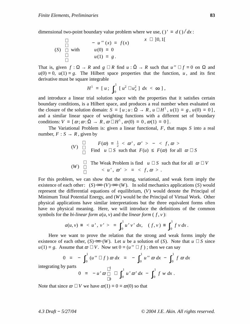
Finite Elements, Preliminaries 83
dimensional two-point boundary value problem where we use, ( )′ = d ( ) / dx :
(S)
with
− u ′′ (x) = f (x)
u(0) = 0
u(1) = g .
x ∈ ]0, 1[
That is, given f : Ω → R and g ∈ R find u : Ω → R such thatu ′′ + f = 0 on Ω andu(0) = 0, u(1) = g. The Hilbert space properties that the function,u , and its firstderivative must be square integrable
H1 = [ u ; ∫1
0[ u2 + u2
x ] dx < ∞ ] ,
and introduce a linear trial solution space with the properties that it satisfies certainboundary conditions, is a Hilbert space, and produces a real number when evaluated onthe closure of the solution domain:S = [ u ; u : Ω → R , u ∈ H1 , u(1) = g , u(0) = 0 ] ,and a similar linear space of weighting functions with a different set of boundaryconditions:V = [ ω ; ω : Ω → R , ω ∈ H1 , ω (0) = 0 , ω (1) = 0 ] .
The Variational Problem is: given a linear functional,F , that mapsS into a realnumber,F : S → R , giv en by
(V)
F(ω ) = 12 < ω ′ , ω ′ > − < f , ω >
Find u ∈ S such thatF(u) ≤ F(ω ) for all ω ∈ S
(W)
The Weak Problem is findu ∈ S such that for allω ∈ V
< u ′ , ω ′ > = < f , ω > .
For this problem, we can show that the strong, variational, and weak form imply theexistence of each other: (S)<===>(V)<===>(W). In solid mechanics applications (S) wouldrepresent the differential equations of equilibrium, (V) would denote the Principal ofMinimum Total Potential Energy, and (W) would be the Principal of Virtual Work. Otherphysical applications have similar interpretations but the three equivalent forms oftenhave no physical meaning. Here, we will introduce the definitions of the commonsymbols for thebi-linear form a(u, v) and thelinear form( f , v ):
a(u, v) ≡ < u ′ , v ′ > = ∫1
0u ′ v ′ dx, ( f , v ) ≡ ∫
1
0f v dx.
Here we want to prove the relation that the strong and weak forms imply theexistence of each other, (S)<===>(W). Let u be a solution of (S). Note thatu ∈ S sinceu(1) = g. Assume thatω ∈ V. Now set 0= (u ′′ + f ) ; then we can say
0 = − ∫1
0(u ′′ + f ) ω dx = − ∫
1
0u ′′ ω dx − ∫
1
0f ω dx
integrating by parts
0 = − u ′ ω
1
0
+ ∫1
0u ′ ω ′ dx − ∫
1
0f w dx .
Note that sinceω ∈ V we haveω (1) = 0 = ω (0) so that
4.3 Draft− 5/27/04 © 2004 J.E. Akin. All rights reserved.
84 J. E. Akin
u ′ ω
1
0
= u ′ (1) ω (1) − u ′ (0)ω (0) ≡ 0 ,
and finally0 = ∫
1
0u ′ ω ′ dx − ∫
1
0f ω dx .
Thus, we conclude thatu(x) is a solution of the weak problem, (W) . That is,a (u, ω ) = ( f , ω ) for all ω ∈ V . Next, we want to verify that the weak solution alsoimplies the existence of the strong form, (W)<===>(S). Assume thatu(x) ∈ S so thatu(0) = 0, u(1) = g, and assume thatω ∈ V :
∫1
0u ′ ω ′ dx = ∫
1
0f ω dx for all ω ∈ V .
Integrating by parts
− ∫1
0( u ′′ + f ) ω dx + u ′ ω
1
0
= 0
but,
u ′ ω
1
0
= u ′ (1) ω (1) − u ′ (0) ω (0) ≡ 0 ,
sinceω ∈ V, and thus
0 = ∫1
0( u ′′ + f ) ω (x) dx , for all ω ∈ V .
Now we pickω (x) ≡ φ (x) (u ′′ + f ) such thatφ produces a real positive number whenevaluated on the domain,φ : Ω → R, and φ (x) > 0, when x ∈ ]0, 1[ andφ (0) = φ (1) = 0. Isω ∈ V? Sinceω (0) = 0 andω (1) = 0, we see that it is and proceedwith that substitution,
0 = ∫1
0( u ′′ + f )2 φ (x) dx = ∫ ( ≥ 0 ) ( > 0 )dx
which implies (u ′′ + f ) ≡ 0. Thus, the weak form does imply the strong form,(W)<===>(S) and combining the above two results we find (S)<===>(W).
Next, we will consider the proposition that the variational form implies the existenceof the weak form, (V)<===>(W). Assumeu ∈ S is a solution to the weak form (W) andnote thatv (1) = ω (1) + u (1) = 0 + g. Therefore,v ∈ S. Now setω = v − u suchthatv = ω + u, andω ∈ V. Giv enF(v) = 1
2 < v ′, v ′ > − < f , v > and expanding
F(v) = F(u + ω ) = 12 < ( u ′ + ω ′ ) , ( u ′ + ω ′ ) > − < f , u + ω >
= 12 < u ′ , u ′ > + < u ′ , ω ′ > + 1
2 < ω ′ , ω ′ > .
But, sinceu is a solution to (W) we hav e <u ′ ,ω ′ > − < f , ω > ≡ 0 , and theabove simplifies toF(v) = F(u) + 1
2 < ω ′, ω ′ > so thatF(v) ≥ F(u) for all v ∈S since< ω ′, ω ′ > ≥ 0. This shows thatu is also a solution of the variational form, (V) . Thatis, (W)<===>(V), which is what we wished to show. Finally, we verify the uniqueness ofthe weak form, (W) . Assume that there are two solutionsu1 andu2 that are both in thespaceS. Then we have botha ( u1 , v ) = ( f , v) , and a ( u2 , v ) = ( f , v) for all v ∈Vand subtracting the second from the first result yieldsa ( u1 − u2 , v ) = 0 , so< ( u1 ′ − u2 ′ ), v ′ > = 0 for all v ∈V . Consider the choicev(x) ≡ u1 (x) − u2 (x) .
4.3 Draft− 5/27/04 © 2004 J.E. Akin. All rights reserved.
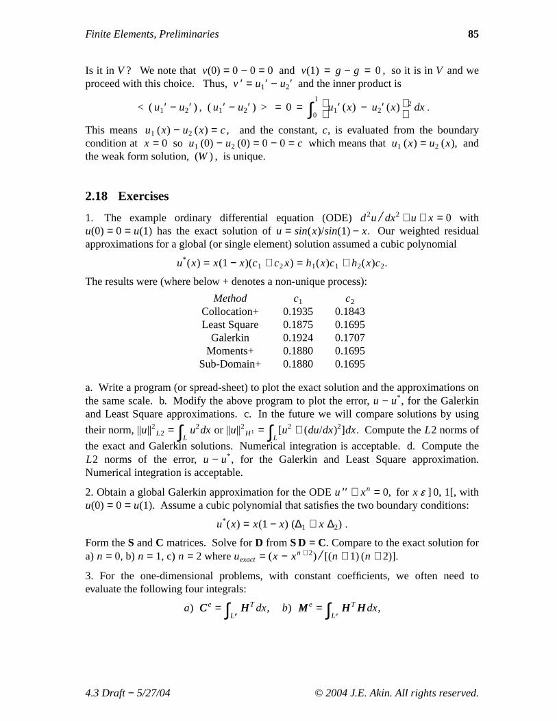
Finite Elements, Preliminaries 85
Is it in V ? We note thatv(0) = 0 − 0 = 0 and v(1) = g − g = 0 , so it is inV and weproceed with this choice. Thus,v ′ = u1′ − u2′ and the inner product is
< ( u1′ − u2′ ) , ( u1′ − u2′ ) > = 0 = ∫1
0
u1′ (x) − u2′ (x)
2 dx .
This meansu1 (x) − u2 (x) = c, and the constant,c, is evaluated from the boundarycondition at x = 0 so u1 (0) − u2 (0) = 0 − 0 = c which means thatu1 (x) = u2 (x), andthe weak form solution, (W) , is unique.
2.18 Exercises
1. The example ordinary differential equation (ODE)d2u/ dx2 + u + x = 0 withu(0) = 0 = u(1) has the exact solution ofu = sin(x)/sin(1) − x. Our weighted residualapproximations for a global (or single element) solution assumed a cubic polynomial
u* (x) = x(1 − x)(c1 + c2x) = h1(x)c1 + h2(x)c2.
The results were (where below + denotes a non-unique process):
Method c1 c2
Collocation+ 0.1935 0.1843Least Square 0.1875 0.1695
Galerkin 0.1924 0.1707Moments+ 0.1880 0.1695
Sub-Domain+ 0.1880 0.1695
a. Write a program (or spread-sheet) to plot the exact solution and the approximations onthe same scale. b. Modify the above program to plot the error,u − u* , for the Galerkinand Least Square approximations. c. In the future we will compare solutions by using
their norm, ||u||2L2 = ∫Lu2dx or ||u||2H1 = ∫L
[u2 + (du/dx)2]dx. Compute theL2 norms of
the exact and Galerkin solutions. Numerical integration is acceptable. d. Compute theL2 norms of the error,u − u* , for the Galerkin and Least Square approximation.Numerical integration is acceptable.
2. Obtain a global Galerkin approximation for the ODEu ′′ + xn = 0, for x ε ] 0, 1[, withu(0) = 0 = u(1). Assume a cubic polynomial that satisfies the two boundary conditions:
u* (x) = x(1 − x) (∆1 + x ∆2) .
Form theS andC matrices. Solve forD from S D = C. Compare to the exact solution fora) n = 0, b)n = 1, c)n = 2 whereuexact = (x − xn + 2) / [(n + 1) (n + 2)].
3. For the one-dimensional problems, with constant coefficients, we often need toevaluate the following four integrals:
a) CCe = ∫LeHHT dx, b) MMe = ∫Le
HHT HH dx,
4.3 Draft− 5/27/04 © 2004 J.E. Akin. All rights reserved.
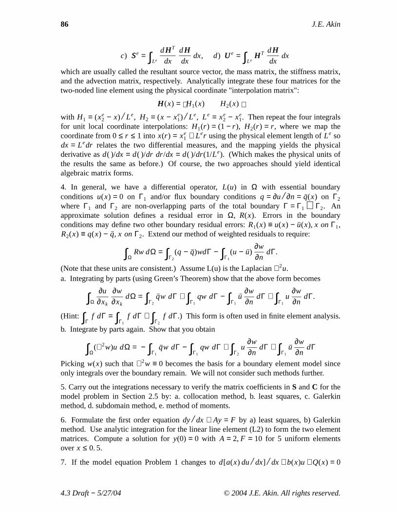
86 J. E. Akin
c) SSe = ∫Le
dHHT
dx
dHH
dxdx , d) UUe = ∫Le
HHT dHH
dxdx
which are usually called the resultant source vector, the mass matrix, the stiffness matrix,and the advection matrix, respectively. Analytically integrate these four matrices for thetwo-noded line element using the physical coordinate "interpolation matrix":
HH(x) = H1(x) H2(x) with H1 = (xe
2 − x) / Le, H2 = (x − xe1) / Le, Le = xe
2 − xe1. Then repeat the four integrals
for unit local coordinate interpolations:H1(r ) = (1 − r ), H2(r ) = r , where we map thecoordinate from 0≤ r ≤ 1 into x(r ) = xe
1 + Ler using the physical element length ofLe sodx = Ledr relates the two differential measures, and the mapping yields the physicalderivative asd( )/dx = d( )/dr dr/dx = d( )/dr(1/Le). (Which makes the physical units ofthe results the same as before.) Of course, the two approaches should yield identicalalgebraic matrix forms.
4. In general, we have a differential operator,L(u) in Ω with essential boundaryconditions u(x) = 0 on Γ1 and/or flux boundary conditionsq = ∂u/ ∂n = q(x) on Γ2
where Γ1 and Γ2 are non-overlapping parts of the total boundaryΓ = Γ1 ∪ Γ2. Anapproximate solution defines a residual error inΩ, R(x). Errors in the boundaryconditions may define two other boundary residual errors:R1(x) ≡ u(x) − u(x), x on Γ1,R2(x) ≡ q(x) − q, x onΓ2. Extend our method of weighted residuals to require:
∫ΩRw dΩ = ∫Γ2
(q − q)wdΓ − ∫Γ1
(u − u)∂w
∂ndΓ.
(Note that these units are consistent.) Assume L(u) is the Laplacian∇2u.a. Integrating by parts (using Green’s Theorem) show that the above form becomes
∫Ω
∂u
∂xk
∂w
∂xkdΩ = ∫Γ2
qw dΓ + ∫Γ1
qw dΓ − ∫Γ1
u∂w
∂ndΓ + ∫Γ1
u∂w
∂ndΓ.
(Hint: ∫Γf dΓ = ∫Γ1
f dΓ + ∫Γ2
f dΓ.) This form is often used in finite element analysis.
b. Integrate by parts again. Show that you obtain
∫Ω(∇2w)u dΩ = − ∫Γ1
qw dΓ − ∫Γ1
qw dΓ + ∫Γ2
u∂w
∂ndΓ + ∫Γ1
u∂w
∂ndΓ
Picking w(x) such that∇2w ≡ 0 becomes the basis for a boundary element model sinceonly integrals over the boundary remain. We will not consider such methods further.
5. Carry out the integrations necessary to verify the matrix coefficients inS andC for themodel problem in Section 2.5 by: a. collocation method, b. least squares, c. Galerkinmethod, d. subdomain method, e. method of moments.
6. Formulate the first order equationdy/ dx + Ay = F by a) least squares, b) Galerkinmethod. Use analytic integration for the linear line element (L2) to form the two elementmatrices. Compute a solution fory(0) = 0 with A = 2,F = 10 for 5 uniform elementsover x ≤ 0. 5.
7. If the model equation Problem 1 changes tod[a(x) du/ dx] / dx + b(x)u + Q(x) = 0
4.3 Draft− 5/27/04 © 2004 J.E. Akin. All rights reserved.
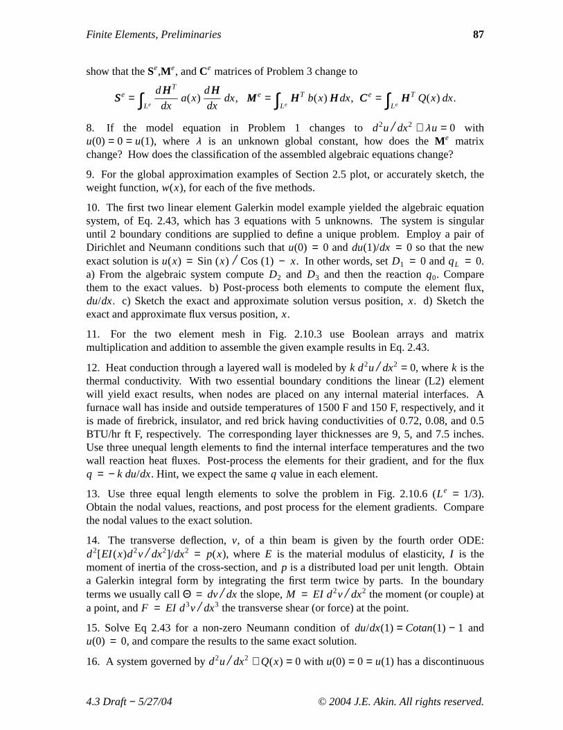
Finite Elements, Preliminaries 87
show that theSe,M e, andCe matrices of Problem 3 change to
SSe = ∫Le
dHHT
dxa(x)
dHH
dxdx , MMe = ∫Le
HHT b(x) HH dx, CCe = ∫LeHHT Q(x) dx.
8. If the model equation in Problem 1 changes tod2u/ dx2 + λu = 0 withu(0) = 0 = u(1), where λ is an unknown global constant, how does theM e matrixchange? How does the classification of the assembled algebraic equations change?
9. For the global approximation examples of Section 2.5 plot, or accurately sketch, theweight function,w(x), for each of the five methods.
10. The first two linear element Galerkin model example yielded the algebraic equationsystem, of Eq. 2.43, which has 3 equations with 5 unknowns. The system is singularuntil 2 boundary conditions are supplied to define a unique problem. Employ a pair ofDirichlet and Neumann conditions such thatu(0) = 0 anddu(1)/dx = 0 so that the newexact solution isu(x) = Sin (x) / Cos (1) − x. In other words, setD1 = 0 andqL = 0.a) From the algebraic system computeD2 and D3 and then the reactionq0. Comparethem to the exact values. b) Post-process both elements to compute the element flux,du/dx. c) Sketch the exact and approximate solution versus position,x. d) Sketch theexact and approximate flux versus position,x.
11. For the two element mesh in Fig. 2.10.3 use Boolean arrays and matrixmultiplication and addition to assemble the given example results in Eq. 2.43.
12. Heat conduction through a layered wall is modeled byk d2u/ dx2 = 0, wherek is thethermal conductivity. With two essential boundary conditions the linear (L2) elementwill yield exact results, when nodes are placed on any internal material interfaces. Afurnace wall has inside and outside temperatures of 1500 F and 150 F, respectively, and itis made of firebrick, insulator, and red brick having conductivities of 0.72, 0.08, and 0.5BTU/hr ft F, respectively. The corresponding layer thicknesses are 9, 5, and 7.5 inches.Use three unequal length elements to find the internal interface temperatures and the twowall reaction heat fluxes. Post-process the elements for their gradient, and for the fluxq = − k du/dx. Hint, we expect the sameq value in each element.
13. Use three equal length elements to solve the problem in Fig. 2.10.6 (Le = 1/3).Obtain the nodal values, reactions, and post process for the element gradients. Comparethe nodal values to the exact solution.
14. The transverse deflection,v, of a thin beam is given by the fourth order ODE:d2[EI (x)d2v / dx2]/dx2 = p(x), whereE is the material modulus of elasticity,I is themoment of inertia of the cross-section, andp is a distributed load per unit length. Obtaina Galerkin integral form by integrating the first term twice by parts. In the boundaryterms we usually callΘ = dv/ dx the slope,M = EI d2v / dx2 the moment (or couple) ata point, andF = EI d3v / dx3 the transverse shear (or force) at the point.
15. Solve Eq 2.43 for a non-zero Neumann condition ofdu/dx(1) = Cotan(1) − 1 andu(0) = 0, and compare the results to the same exact solution.
16. A system governed byd2u/ dx2 + Q(x) = 0 with u(0) = 0 = u(1) has a discontinuous
4.3 Draft− 5/27/04 © 2004 J.E. Akin. All rights reserved.

88 J. E. Akin
source value ofQ = 1 for x ≤ 1/2 and 0 forx > 1/2. a) Explain why it is preferable foran element end to be placed atx = 1/2. b) If you used 3 linear (L2) elements explain whyit is better to place the two smaller elements in the left half of the domain. c) If you usethat mesh verify that the (exact) interior nodal values are 5/72 and 1/24. d) If instead youuse 3 elements of constant length (Le = 1/3) verify that the source vector for the secondelement isCeT = [3 1]/24 and that the (exact) interior nodal values are each 1/16.
17. Obtain a Galerkin solution ofy′′ − 2y′x / g + 2y / g = g, for g = (x2 + 1), on0 ≤ x ≤ 1 with the boundary conditionsy(0) = 2, y(1) = 5 / 3.
18. For the differential equation in Problem 2.17 if we have one essential boundarycondition ofy(0) = 1 and one Neumann flux boundary condition ofdy/dx(1) = − 4/3 theexact solution is unchanged. Obtain a Galerkin finite element solution and compare it tothe exact result.
19. The Couette steady flow velocity,u, of an incompressible viscous fluid between twoparallel plates, with a constant pressure gradient ofdP/ dx, is: µd2u/ dy2 = dP/ dx,whereu(0) = 0 andu(H) = UH describe a lower (y = 0) fixed plate and an upper plate(y = −h) moving with a speed ofUH . One can obtain a finite element solution for theinterior nodal velocites across the fluid. The associated volume flow, per unitz thickness,
is Q = ∫H
0u(y)dy. Describe how you would post-process the elements to obtain it.
20. For the above Couette flow would you expect to obtain the exactu(y) andQ valuesfor a) one quadratic element, b) two quadratic elements, c) two linear elements? Explainwhy.
21. Differences between Galerkin and least squares finite element procedures are_______: a) Galerkin allows integration by parts, b) least squares always yield symmetricalgebraic equations, c) least squares requiresC1 continuity for second order differentialequations, d) all of the above.
22. Repeat the graphical source assembly shown in Fig. 2.10.3 using three elementsinstead of two.
23. Burnett presents detailed studies of a symmetric bi-material bar with not-symmetricalboundary conditions. The total bar length isL = 100cm with the center-most 20cmsection being constructed out of copper (kc = 0. 92cal / sec− cm− C, ρ = 8. 5gm/ cm3,cp = 0. 092cal / gm− C) while the other two ends of the bar are made of 40cm of steel(kc = 0. 12cal / sec− cm− C, ρ = 7. 8gm/ cm3, cp = 0. 11cal / gm− C). The circularbar has a radius of 2cm. Along its full length it convects to surrounding air atU∞ = 20C. The end area atx = 0 receives a flux ofq = 0. 1cal / sec− cm2 and the endat x = 100 has a temperature ofU100 = 0C. Obtain: a) a steady state solution with 5equal length elements, b) a transient solution assuming an initial condition ofU(x, 0) = 20C. Note that the two end "thermal shocks" will require a finer mesh at theends if the early time history is important. Would the steady state solution also need thatmesh feature?
4.3 Draft− 5/27/04 © 2004 J.E. Akin. All rights reserved.
Finite Elements, Preliminaries 89
2.19 Bibliography
[1] Adams, R.A.,Sobolev Spaces, New York: Academic Press (1975).[2] Ainsworth, M. and Oden, J.T.,A Posteriori Error Estimation in Finite Element
Analysis, New York: John Wiley (2000).[3] Akin, J.E., Finite Elements for Analysis and Design, London: Academic
Press (1994).[4] Axelsson, O. and Baker, V.A.,Finite Element Solution of Boundary Value Problems,
Philadelphia, PA: SIAM (2001).[5] Aziz, A.K., The Mathematical Foundations of the Finite Element Method with
Applications to Partial Differential Equations, New York: Academic Press (1972).[6] Bonnerot, R. and Jamet, P., "Numerical Computation of the Free Boundary for the
Tw o-Dimensional Stefan Problem by Space-Time Finite Elements,"J.Computational Physics, 25, pp. 163−181 (1977).
[7] Bruch, J.C. Jr. and Zyvoloski, G., "Transient Two - Dimensional Heat ConductionProblems Solved by the Finite Element Method,"Int. J. Num. Meth. Eng., 8,pp. 481−494 (1974).
[8] Buchanan, G.R.,Finite Element Analysis, New York: McGraw-Hill (1995).[9] Ciarlet, P.G.,The Finite Element Method for Elliptical Problems, Philadelphia, PA:
SIAM (2002).[10] DeBoor, C., ed.,Mathematical Aspects of Finite Elements in Partial Differential
Equations, London: Academic Press (1974).[11] Desai, C.S., Elementary Finite Element Method, Englewood Cliffs:
Prentice-Hall (1979).[12] Heinrich, J.C. and Pepper, D.W.,Intermediate Finite Element Method, Philadelphia,
PA: Taylor & Francis (1999).[13] Huang, H.C. and Usmani, A.S., inFinite Element Analysis for Heat Transfer,
London: Springer-Verlag (1994).[14] Hughes, T.J.R., The Finite Element Method, Englewood Cliffs:
Prentice-Hall (1987).[15] Liusternik, L.A. and Sobolev, V.J.,Elements of Functional Analysis, New York:
Frederick Ungar (1961).[16] Meier, D.L., "Multi-Dimensional Astrophysical Structural and Dynamical Analysis,
Development of a Nonlinear Finite Element Approach,"Astrophysics J., 518,pp. 788−813 (1999).
[17] Mitchell, A.R. and Wait, R.,The Finite Element Method in Partial DifferentialEquations, London: John Wiley (1977).
[18] Nowinski, J.L.,Applications of Functional Analysis in Engineering, New York:Plenum Press (1981).
[19] Oden, J.T. and Reddy, J.N.,An Introduction to the Mathematical Theory of FiniteElements, New York: John Wiley (1976).
4.3 Draft− 5/27/04 © 2004 J.E. Akin. All rights reserved.

90 J. E. Akin
[20] Oden, J.T.,Applied Functional Analysis, Englewood Cliffs: Prentice-Hall (1979).[21] Oden, J.T. and Carey, G.F.,Finite Elements: Mathematical Aspects, Prentice
Hall (1983).[22] Oden, J.T., "The Best FEM,"Finite Elements in Analysis and Design, 7,
pp. 103−114 (1990).[23] Reddy, J.N. and Gartling, D.K.,The Finite Element Method in Heat Transfer and
Fluid Dynamics, Boca Raton: CRC Press (2001).[24] Strang, W.G. and Fix, G.J.,An Analysis of the Finite Element Method, Englewood
Cliffs: Prentice-Hall (1973).[25] Szabo, B. and Babuska, I.,Finite Element Analysis, New York: John Wiley (1991).[26] Tezduyar, T.E. and Ganjoo, D.K., "Petrov-Galerkin Formulations with Weighting
Functions Dependent Upon Spatial and Temporal Discretization,"Comp. Meth.Appl. Mech. Eng., 59, pp. 47−71 (1986).
[27] Whiteman, J.R., "Some Aspects of the Mathematics of Finite Elements," pp. 25−42in The Mathematics of Finite Elements and Applications, Vol. II, ed. J.R. Whiteman,London: Academic Press (1976).
[28] Zhu, J.Z. and Zienkiewicz, O.C., "Superconvergence Recovery Techniques andA PosterioriError Estimators,"Int. J. Num. Meth. Eng., 30, pp. 1321−1339 (1990).
[29] Zienkiewicz, O.C. and Morgan, K.,Finite Elements and Approximation, Chichester:John Wiley (1983).
[30] Zienkiewicz, O.C. and Taylor, R.L.,The Finite Element Method,4th Edition, NewYork: McGraw-Hill (1991).
[31] Zienkiewicz, O.C. and Zhu, J.Z., "Superconvergent Patch Recovery Techniques andAdaptive Finite Element Refinement,"Comp. Meth. Appl. Mech. Eng., 101,pp. 207−224 (1992).
[32] Zienkiewicz, O.C. and Zhu, J.Z., "The Superconvergent Patch Recovery anda PosterioriError Estimates. Part 2: Error Estimates and Adaptivity,"Int. J. Num.Meth. Eng., 33, pp. 1365−1382 (1992).
4.3 Draft− 5/27/04 © 2004 J.E. Akin. All rights reserved.