Embed Size (px)
Citation preview
1 Mathematical Preliminaries
We shall go through in this first chapter all of the mathematics needed for reading the rest of this
book.
The reader is expected to have taken a one‐year course in differential and integral calculus.
1.1 Mean‐Value Theorems of Integral Calculus
First mean‐value theorem of integral calculus
Let be continuous on , and 0 (or 0) in , .
Then,
,
where is in , .
Proof
We shall prove the case for 0; the case for 0 is entirely analogous.
Since is continuous on , , it is bounded, i.e., there exist and such that
for all in , .
We further have for all in , since 0 for all in
, .
Hence,
.
1; . 1
Since is continuous on , , it must evolve continuously between and .
Hence, for any satisfying , there exists an in , such that .
Now, apply the above statement to 1 .
Let
1.
1
Since , there exists in , such that .
Hence,
1.
That is,
.
∎
In particular, if 1, we have
.
Second mean‐value theorem of integral calculus
Let be monotonically increasing (or decreasing) on , and be integrable on , .
Then,
,
where is in , .
Proof
We assume first that is monotonically increasing, implying that 0 on , .
Let
^ ^ .
Hence, is differentiable and thus continuous on , .
|
By first mean‐value theorem
2 Chapter 1
.
∎
1.2 The Delta Function
Definition
We define the delta function, denoted conventionally as , to be the limit of a sequence of
functions in the sense that, if
lim⟶
12, 0
or
lim⟶
12, 0,
then
lim⟶
.
Claim
lim⟶
0,
where 0 or 0.
Proof
For 0 ,
lim⟶
lim⟶
lim⟶
12
12
0.
The case for 0 can be proved in a similar way.
∎
1.2.1 Representations of the delta function
1.)
One representation of the delta function is
Mathematical Preliminaries 3

sin, ⟶ ∞.
We use instead of as the index of the sequence of functions since it is not restricted to
integers.
This is because
lim⟶
sinlim⟶
1 sin ^
^^
1 sin ^
^^
12
12.
The evaluation of the last integral is detailed in Appendix 1.1.
To show the reader this trend, we plot the representation for from 1 (blue) to 5 (red) in steps
of 1, as shown in Fig. 1.2‐1.
2.)
Another representation of the delta function is
√, ⟶ ∞.
This is because
lim⟶ √
lim⟶
1
√^ ^
1
√^ ^
1
√
√2
12.
Figure 1.2‐1
4 Chapter 1
3.)
Still another representation of the delta function is
12
, ⟶ ∞.
This is because, by performing the integration
12
12
sin,
we can reduce it to the first representation above.
4.)
Our final example of the representation of the delta function is the following sequence of
polynomials:
1 , | | 1; 0, | | 1, 1, 2, 3,⋯,
where is a normalization factor defined by
112, 1, 2, 3,⋯.
Proof
When 0 1, consider the following integral
1
1 1
12
1 .
On one hand,
1≡ 2 1 2 1 2
11
21;
12
.
On the other hand,
Mathematical Preliminaries 5
1 1 1 1 .
Hence,
11
21 ⟶ 0, ⟶ ∞.
Then,
12.
When 1,
112
by the definition of and .
Therefore,
lim⟶
112, 0,
which means , ⟶ ∞ is indeed a representation of the function.
∎
1.2.2 Properties of the delta function
1.)
Sifting
When 0, if is continuous on 0, and | ⟶ 0 , then
12
0 .
Similarly, when 0, if is continuous on , 0 and | ⟶ 0 , then
12
0 .
In particular,
6 Chapter 1

12
0 0 ,
which is equal to 0 if is continuous at 0.
Proof
We first prove the case of 0.
Since is continuous, there exists a small enough such that is monotonic on 0, .
We then apply the second mean‐value theorem of integral calculus and get
lim⟶
lim⟶
0 lim⟶
0 ∗12
∗ 0.
For 0 in general, we write
12
0 .
Next, we divide , into several sub‐intervals in which is monotonic.
Let one such sub‐interval be , .
Then,
lim⟶
lim⟶
lim⟶
∗ 0 ∗ 0.
Hence, adding up all such integrals, we have
0.
Therefore, when 0,
12
0 .
Mathematical Preliminaries 7
Similarly, when 0,
12
0 .
If is continuous at 0,
12
0 0 0 .
∎
Letting in the above equation , we have
.
By change of variable ^, we obtain
^ ^ ^ .
The above expression is the most common form for expressing the sifting property of the delta
function.
2.)
Scaling
1| |
0 .
Proof
If 0,
^⁄ ^^
10 .
If 0,
^⁄ ^^
1^⁄ ^ ^
8 Chapter 1
10 .
∎
3.)
Functional
1| |
.
Proof
is non‐trivial only in the neighborhood of 0.
Thus, for , we can only focus on those tiny intervals centered at ’s where 0, and
on each such interval, approximate by a linear function, i.e.,
.
Hence,
.
1| |
.
We may then state, equivalently,
1| |
.
∎
4.)
Differentiation
.
Proof
lim⟶
Δ 2⁄ Δ 2⁄
Δ
lim⟶
Δ 2⁄ Δ 2⁄
Δ
lim⟶
Δ 2⁄ Δ 2⁄Δ
.
Mathematical Preliminaries 9
1.3 Weierstrass’ Approximation Theorem
Weierstrass’ approximation theorem states that any function which is continuous in an interval can
be approximated uniformly by polynomials, i.e., 1, , , …, in this interval.
Weierstrass’ approximation theorem can be explained by employing the sifting property of the delta
function we have just proved.
Assume that is continuous in , .
Then,
lim⟶
1 ,
by employing the polynomial representation of the delta function.
Here, .
Why is the integration domain , larger than , ?
If we integrate over , , then at the boundary, e.g., at , we only get 2⁄ , not .
After performing the integration in the above equation, we obtain a polynomial of order 2 .
We need to choose a proper to meet the required error tolerance.
For an explicit proof of Weierstrass’ approximation theorem, see Appendix 1.2.
1.4 Fourier Transform
We define the Fourier transform as
≡
and the inverse Fourier transform as
≡2.
and are called Fourier transform pairs.
The functions and are generally complex; however, the variables and are
always real unless otherwise stated.
10 Chapter 1
1.4.1 Fourier transform theorems
1.)
Fourier integral theorem
.
Proof
2
2
^
.
If is discontinuous at , replace by in the second‐to‐last equation
and let ⟶∞.
We see that the newly obtained is the average of in the neighborhood of .
∎
2.)
Linearity theorem
.
3.)
Scaling theorem
1| |
⁄ .
Proof
If 0,
Mathematical Preliminaries 11
1
1⁄ .
If 0,
1
1⁄ .
∎
4.)
Shift theorem
. Proof
.
∎
12 Chapter 1
5.)
Rayleigh’s (Parseval’s) theorem
| |2.
Proof
| |2 2
∗
2 2∗
2 2∗ 2
2.
∎
6.)
Convolution theorem
The convolution of two functions is defined as
⨂ ≡
⨂ .
Then,
⨂
Mathematical Preliminaries 13
^
. Besides,
2 2
2 2
2 22
either
2
⨂
or
2.
⨂ .
7.)
Complex conjugate
∗ ∗
∗
14 Chapter 1
∗
∗
∗
∗.
That is, the operations of the Fourier transform and complex conjugate do not commute unless
, i.e., for functions with inversion symmetry.
8.)
Autocorrelation theorem
⨂ ∗ ∗ ∗ .
In addition,
| | ∗ ⨂ ∗ ⨂ ∗ .
1.4.2 Useful Fourier transform pairs
1.)
Fourier transform of the rectangle function
The rectangle function in the real space of width is defined as
Rect ⁄1, | | 2⁄
1 2⁄ , | | 2⁄0, | | 2⁄ .
Finding its Fourier transform is straightforward:
Rect ⁄
⁄
⁄
⁄
⁄
⁄ ⁄
2 sin 2⁄
Mathematical Preliminaries 15
sin 2⁄
2⁄
Sinc 2⁄ .
The rectangular function in the frequency space may be employed more frequently.
Similarly, it can be shown that
Rect ⁄2
Sinc 2⁄ .
2.)
Fourier transform of the comb function
The comb function is defined as
,
which is a periodic function of period .
We want to compute its Fourier transform.
∗ ∗
∗ ∗
∗ ∗ is a periodic function of period 2 ⁄ . ∗ ∗ is a periodic function of period 2 2⁄ , which is also a periodic function of period 2 ⁄ .
…
Therefore, is also a periodic function of period 2 ⁄ .
lim⟶
lim⟶
11
lim⟶ 1
⁄ ⁄ ⁄
16 Chapter 1
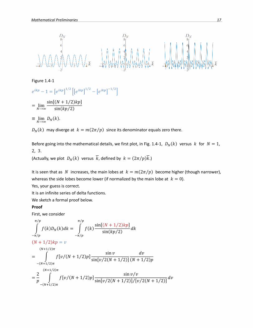
Figure 1.4‐1
1⁄ ⁄ ⁄
lim⟶
sin 1 2⁄sin 2⁄
≡ lim⟶
.
may diverge at 2 ⁄ since its denominator equals zero there.
Before going into the mathematical details, we first plot, in Fig. 1.4‐1, versus for 1,
2, 3.
(Actually, we plot versus , defined by 2 ⁄ .)
It is seen that as increases, the main lobes at 2 ⁄ become higher (though narrower),
whereas the side lobes become lower (if normalized by the main lobe at 0).
Yes, your guess is correct.
It is an infinite series of delta functions.
We sketch a formal proof below.
Proof
First, we consider
⁄
⁄
sin 1 2⁄
sin 2⁄
⁄
⁄
1 2⁄
1 2⁄⁄sin
sin 2 1 2⁄⁄ 1 2⁄
⁄
⁄
21 2⁄⁄
sin ⁄
sin 2 1 2⁄⁄ 2 1 2⁄⁄⁄
⁄
⁄
Mathematical Preliminaries 17
lim⟶
sin 2 1 2⁄⁄
2 1 2⁄⁄lim⟶
sin1
⟶2
0sin
, ⟶ ∞
40
sin
sin2
20 .
Since is a periodic function of period 2 ⁄ ,
lim⟶
22 ⁄ .
∎
Computing the inverse Fourier transform of the above equation, we obtain
2
12 ⁄
1 ∗ ∗.
In summary,
1 ∗ ∗;
∗ ∗ 22 ⁄ . 1
18 Chapter 1