1

Chapter 1 Structure of Power Systems

1.1 Power Systems

Generation, Transmission and Distribution systems are the

main components of an electric power system. Generating

stations and distribution systems are connected through

transmission lines. Normally, transmission lines imply the

bulk transfer of power by high-voltage links between main load

centers. On the other hand, distribution system is mainly

responsible for the conveyance of this power to the consumers

by means of lower voltage networks. Electric power is

generated in the range of 11 kV to 25 kV, which is increased

by stepped up transformers to the main transmission voltage.

At sub-stations, the connections between various components

are made, for example, lines and transformers and switching of

these components is carried out. Transmission level voltages are

in the range of 66 kV to 400 kV (or higher). Large amounts of

power are transmitted from the generating stations to the load

centers at 220 kV or higher. In USA it is at 345 kV, 500 kV and

765 kV, in Britain, it is at 275 kV and 400 kV and in Egypt it is

at 500 kV and 750 kV. The network formed by these very high

2

voltage lines is sometimes called as the super grid. This grid, in

turn, feeds a sub-transmission network operating at 132 kV or

less. In Egypt, networks operate at 132 kV, 66 kV, 33 kV, 11

kV or 6.6 kV and supply the final consumer feeders at 380 volt

three phase, giving 220 volt per phase.

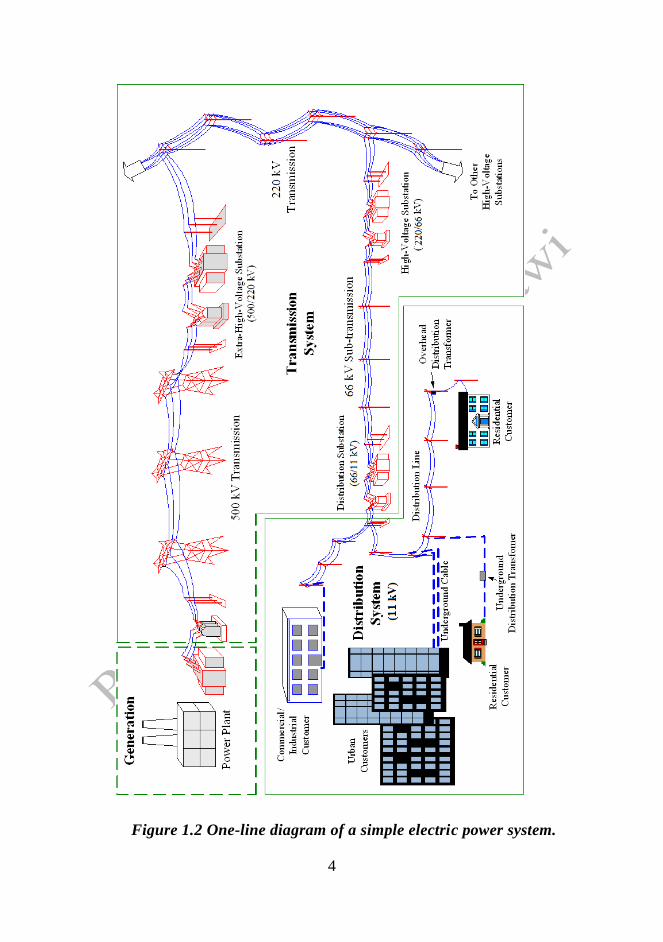
Figure 1.1 and Figure 1.2 shows the schematic diagram of a

power supply network. The power supply network can be

divided into two parts, i.e., transmission and distribution

systems. The transmission system may be divided into primary

and secondary (sub-transmission) transmission system.

Distribution system can be divided into primary and

secondary distribution system. Most of the distribution

networks operate radially for less short circuit current and

better protective coordination.

Distribution networks are different than transmission networks

in many ways, quite apart from voltage magnitude. The general

structure or topology of the distribution system is different and

the number of branches and sources is much higher. A

typical distribution system consists of a step-down

transformer (e.g., 132/11 kV or 66/11 kV or 33/11 kV) at a bulk

supply point feeding a number of lines with varying length

from a few hundred meters to several kilometers. Several

three-phase step-down transformers, e.g., 11 kV/400 V are

spaced along the feeders and from these, three-phase four-wire

3

networks of consumers are supplied which give 220 volt

single-phase supply to houses and similar loads. Figure 1.3

shows part of a typical power system.

Figure 1.1 Schematic diagram of a power supply system.

4

Figure 1.2 One-line diagram of a simple electric power system.

5

Figure 1.3: Part of a typical power system.

1.2 Reasons for Interconnection

Generating stations and distribution systems are connected

through transmission lines. The transmission system of a

particular area (e.g., state) is known as a grid. Different grids

are interconnected through tie-lines to form a regional grid

(also called power pools). Different regional grids are further

connected to form a national grid. Cooperative assistance is

one of the planned benefits of interconnected operation.

6

Interconnected operation is always economical and reliable.

Generating stations having large MW capacity are available to

provide base or intermediate load. These generating stations

must be interconnected so that they feed into the general

system but not into a particular load. Economic advantage of

interconnection is to reduce the reserve generation capacity in

each area. If there is sudden increase of load or loss of

generation in one area, it is possible to borrow power from

adjoining interconnected areas. To meet sudden increases in

load, a certain amount of generating capacity (in each area)

known as the "spinning reserve" is required. This consists of

generators running at normal speed and ready to supply power

instantaneously.

It is always better to keep gas turbines and hydro

generators as "spinning reserve". Gas turbines can be started

and loaded in 3 minutes or less. Hydro units can be even

quicker. It is more economical to have certain generating

stations serving only this function than to have each station

carrying its own spinning reserve. Interconnected operation

also gives the flexibility to meet unexpected emergency loads.

1.3 Load Types

Total load demand of an area depends upon its population

and the living standards of people. General nature of load is

characterized by the load factor, demand factor, diversity

7

factor, power factor and utilization factor. In general, the

types of load can be divided into the following categories:

(1) Domestic (2) Commercial (3) Industrial (4) Agriculture.

Domestic Load: Domestic load mainly consists of lights, fans,

refrigerators, air-conditioners, mixer, grinders, heaters, ovens,

small pumping motors etc.

Commercial Load: Commercial load mainly consists of

lighting for shops, offices, advertisements etc., fans, heating, air-

conditioning and many other electrical appliances used in

commercial establishments such as market places, restaurants

etc.

Industrial Loads: Industrial loads consist of small-scale

industries, medium-scale industries, large-scale industries,

heavy industries and cottage industries.

Agriculture Loads: This type of load is mainly motor pump-

sets load for irrigation purposes. Load factor for this load is

very small, e.g., 0.15-0.20.

1.4 Load Curves

The curve showing the variation of load on the power

station with reference to time is known as a load curve.

The load on a power station is never constant; it varies

from time to time. These load variations during the whole day

(i.e. 24 hours) are recorded half-hourly or hourly and are

plotted against time on the graph. The curve thus obtained is

8

known as daily load curve as it shows the variations of load

with reference to time during the day. Fig. 1.4 shows a typical

daily load curve of a power station. It is clear that load on the

power station is varying, being maximum at 6 P.M. in this

case. It may be seen that load curve indicates at a glance the

general character of the load that is being imposed on the

plant. Such a clear representation cannot be obtained from

tabulated figures.

Fig. 1.4 daily load curve

The monthly load curve can be obtained from the daily

load curves of that month. For this purpose, average values of

power over a month at different times of the day are calculated

and then plotted on the graph. The monthly load curve is

generally used to fix the rates of energy. The load curve is

obtained by considering the monthly load curves of that

particular year. The yearly load curve is generally used to

9

determine the annual load factor.

Important Notes:

The daily load curves have attained a great importance in

generation as they supply the following information readily:

i. The daily load curve shows the variations of load on the

power station during different hours of the day.

ii. The area under the load curve gives the number of units

generated in the day.

Units generated/day = Area (in kWh) under daily load curve.

iii. The highest point on the load curve represents the

maximum demand on the station on that day.

iv. The area under the load curve divided by the total

number of hours gives the average load on the station.

v. The ratio of the area under the load curve to the total

area of rectangle in which it is contained gives the load

factor.

vi. The load curve helps in selecting the size number of

generating units.

10

1.5 Units Generated per Annum

It is often required to find the kWh generated per annum

from maximum demand and load factor.

1.6. Base Load and Peak Load on Power Station

The changing load on the power station makes its load

curve of variable nature. Figure 1.4, shows the typical load

curve of a power station. It is clear that load on the power

station varies from time to time. The load curve shows that

load on the power station can be considered in two parts,

namely; (i) Base load (ii) Peak load

Base load: The unvarying load which occurs almost the

whole day on the station. Referring to the load curve of

Fig. 1.5, it is clear that 20 MW of load has to be supplied

by the station at all times of day and night i.e. throughout

24 hours. Therefore, 20 MW is the base load of the

station. As base load on the station is almost of constant

nature, therefore, it can be suitably supplied (as discussed

in the next Article) without facing the problems of

variable load.

11

Peak load: The various peak demands of load over and

above the base load of the station. Referring to the load

curve of Fig. 1.5, it is clear that there are peak demands

of load excluding base load. These peak demands of the

station generally form a small part of the total load and

may occur throughout the day.

Fig. 1.5

1.7. Method of Meeting the Load

The total load on a power station consists of two parts:

base load and peak load. In order to achieve overall economy,

the best method to meet load is to interconnect different power

stations. The more efficient plants are used to supply the base

load and are known as base load power stations. The less

efficient plants are used to supply the peak loads and is known

12

as peak load power stations. There is no hard and fast rule for

selection of base load and peak load stations as it would

depend upon the particular situation. For example, both hydro-

electric and steam power stations are quite efficient and can be

used as base load as well as peak load station to meet a

particular load requirement.

Illustration: The interconnection of steam and hydro

plants is a beautiful illustration to meet the load. When water

is available in sufficient quantity as in summer and rainy

season, the hydroelectric plant is used to carry the base load

and the steam plant supplies the peak load as shown in

Fig 1.6 (i). However, when the water is not available in

sufficient quantity as in winter, the steam plant carries the

base load, whereas the hydro-electric plant carries the peak

load as shown in Fig. 1.6 (ii)

Fig. 1.6 Load division on Hydro-steam system

13

1.8 Load duration Curve

When the load elements of a load curve are arranged in the

order of descending magnitudes, the curve thus obtained is

called a load duration curve.

The load duration curve is obtained from the same data as

the load curve but the ordinates are arranged in the order of

descending magnitudes. In other words, the maximum load is

represented to the left and decreasing loads are represented to

the right in the descending order. Hence the area under the

load duration curve and the area under the load curve are

equal. Fig. 1.7 (i) shows the daily load curve. The daily load

duration curve can be readily obtained from it.

Fig.1.7 Daily load duration curve

It is clear from daily load curve [See Fig. 1.7. (i)], that load

elements in order of descending magnitude are : 20 MW for 8

hours; 15 MW for 4 hours and 5 MW for 12 hours. Plotting

14

these loads in order of descending magnitude, we get the daily

load duration curve as shown in Fig. 1.7 (ii).

Here are some important points about load duration curve:

The load duration curve gives the data in a more

presentable form. In other words, it readily shows the

number of hours during which the given load has

prevailed.

The area under the load duration curve is equal to that of

the corresponding load curve. Obviously, area under

daily load duration curve. Obviously, area under daily

load duration curve (in kWh) will give the units

generated on that day.

The duration curve can be extended to include any

period of time. By laying out the abscissa from 0 hour to

8760 hours, the variation and distribution of demand for

an entire year can be summarized in one curve. The

obtained curve is called the annual load duration curve.

1.9 Basic Definitions of Commonly Used Terms

Electrical engineers use the following terms and factors to

describe energy flow in power systems:

Connected load: It is the sum of continuous ratings of all

the equipment connected to supply system.

A power station supplies load to thousands of consumers.

15

Each consumer has certain equipment installed in his

premises. The sum of the continuous ratings of all the

equipments in the consumer’s premises is the “connected

load‖ of the consumer. For instance, if a consumer has

connections of five 100-watt lamps and a power point of 500

watts, then connected load of the consumer is 5 x 100 + 500 =

1000 watts. The sum of the connected loads of all the

consumers is the connected load to the power station.

Maximum demand: It is the greatest demand of load on the

power station during a given period.

The load on the power station varies from time to time.

The maximum of all the demands that have occurred during a

given period (say a day) is the maximum demand. Thus

referring back to the load curve of Fig. 1.4 the maximum

demand on the power station during the day is 6 MW and it

occurs at 6 P.M. Maximum demand is generally less than the

connected load because all the consumers do not switch on

their connected load to the system at a time. The knowledge of

maximum demand is very important as it helps in determining

the installed capacity of the station. The station must be

capable of meeting the maximum demand.

16

Demand factor. It is the ratio of maximum demand on the

power station to its connected load i.e.

The value of demand factor is usually less than 1. It is

expected because maximum demand on the power station

generally less than the connected load. If the maximum

demand on the power station is 80 MW and the connected load

is 100 MW, then demand factor = 80/100 = 0.8. The

knowledge of demand factor is vital in determining the

capacity of the plant equipment.

Average load. The average of loads occurring on the power

station in a given period (day or month or year) is known as

average load or average demand.

Load factor. The ratio of average load to the maximum

demand during a given period is known as load factor.

17

If the plant is in operation for T hours,

The load factor may be daily load factor, monthly load

factor or annual load factor if the time period considered is a

day or month or year. Load factor is always less than 1

because average load is smaller than the maximum demand.

The load factor plays key role in determining the overall cost

per unit generated. Higher the load factor of the power

station, lesser will be the cost per unit generated (It is because

higher load factor means lesser maximum demand. The station

capacity is so selected that it must meet the maximum

demand. Now, lower maximum demand means lower capacity

of the plant which, therefore, reduces the cost of the plant).

Diversity factor. The ratio of the sum of individual

maximum demands to the maximum demand on power

station is known as diversity factor i.e.

A power station supplies load to various types of

consumers whose maximum demands generally do not occur

at the same time. Therefore, the maximum demand on the

18

power station is always less than the sum of individual

maximum demands of the consumers. Obviously, diversity

factor will always be greater than 1. The greater the diversity

factor, the lesser is the cost of generation of power (Greater

diversity factor means lesser maximum demand. This in turn

means that lesser plant capacity is required. Thus, the capital

investment on the plant is reduced).

Capacity factor. It is the ratio of actual energy produced to

the maximum possible energy that could have been

produced during a given period i.e.

Suppose the period is T hours then:

Thus if the considered period is one year,

The plant capacity factor is an indication of the reserve

capacity of the plant. A power station is so designed that it has

some reserve capacity for meeting the increased load demand

in future.

19

Therefore, the installed capacity of the plant is always

somewhat greater than the maximum demand on the plant.

Reserve capacity = Plant capacity - Max. demand.

It is interesting to note that difference between load factor

and capacity factor is an indication of reserve capacity. If the

maximum demand on the plant is equal to the plant capacity,

then load factor and plant capacity factor will have the same

value. In such a case, the plant will have no reserve capacity.

Plant use factor. It is the ratio of kWh generated to the

product of plant capacity and the number of hours for which

the plant was in operation i.e.

Suppose a plant having installed capacity of 20 MW produces

annual output of 7.35 x 106 kWh and remains in operation for

2190 hours in year. Then:

20

Solved Examples

Example 1.1: A diesel station supplies the following loads to

various consumers:

Industrial consumer=1500 kW; Commercial establishment = 750 kW

Domestic power = 100 kW; Domestic light = 450 kW

If the maximum demand on the station is 2500 kW and the

number of kWh generated per year is 45 × 105, determine

(i) the diversity factor and (ii) annual load factor.

Solution:

(i) Diversity factor = (1500 + 750 + 100 + 450)/2500 = 1·12

(ii) Average demand = yearly kWh generated/Hours in a year

= 45×105/8760 = 513.7 kW

Load factor = Average load/Max. demand = 513.7/2500

= 0·205 = 20·5%

Example 1.2: A power station supplies the following load

Time (hours) Load (MW)

6 AM — 8 AM 1.2

8 AM — 9 AM 2.0

9 AM — 12 Noon 3.0

12 Noon — 2 PM 1.50

2 PM — 6 PM 2.50

6 PM — 8 PM 1.80

8 PM — 9 PM 2.0

9 PM — 11 PM 1.0

11 PM — 5 AM 0.50

5 AM — 6 AM 0.80

21

(a) Plot the load curve and find out the load factor.

(b) Determine the proper number and size of generating

units to supply this load.

(c) Find the reserve capacity of the plant and capacity

factor.

(d) Find out the operating schedule of the generating units

selected.

Solution:

(a) The following figure shows the plot of load curve

Units generated during 24 hours =(2x1.2 +1x2+3x3+2 x 1.5+

4x2.5 + 2x1.8 + 1x2 + 2x1 + 6x0.5 + 1x0.8) = 37.80 MWhr

Average load = Units generated / Time in hours

Average load = 37.80 / 24 = 1.575 MW.

Load factor (LF) = Maximum load / Maximum load

Maximum load = 3 MW LF = 1.575/3 = 0.525

(b) Maximum demand = 3 MW. Therefore, 4 generating units

of rating 1.0 MW each may be selected. During the period of

22

maximum demand 3 units will operate and 1 unit will remain

as stand by.

(c) Plant capacity = 4 x 1.0 = 4.0 MW

Reserve capacity = 4 - 3 = 1 MW

From eqn. (1.3),

Actual energy produced = 37.80 MWhr

Maximum plant rating = 4 MW

Time duration T = 24 hours

Plant Capacity Factor = 37.80/(4 x 24) = 0.39375.

(d) Operating schedule will be as follows:

One generating unit of 1 MW: — 24 hours

Second generating unit of 1 MW: — 6 AM — 9 PM

(15 hours)

Third generating unit of 1 MW: — 9 AM — 12 Noon

2 PM — 6 PM

(7 hours)

Example 1.3: A generating station has the following daily

load cycle:

Time (Hours) 0 —6 6—10 10 —12 12 —16 16 —20 20 —24

Load(M W) 40 50 60 50 70 40

Draw the load curve and find (i) maximum demand (ii) units

generated per day (iii) average load and (iv) load factor.

23

Solution:

Daily curve is drawn by taking the load along Y-axis and

time along X-axis and is shown in Figure.

(i) It is clear from the load curve that maximum demand on

the power station is 70 MW and occurs during the period 16-

20 hours. ∴ Maximum demand = 70 MW

(ii) Units generated/day = Area (in kWh) under the load curve

= 103 [40×6 + 50×4 + 60×2 + 50×4 + 70×4 + 40×4]

= 12 × 105 kWh

(iii) Average load = Units generated per day/24 hours

=12 ×105/ 24 = 50,000 kW

(iv) Load factor =Average load/Max. demand = 50 000/70×103

= 0·714

Example 1.4: A power station has to meet the following

demand: Group A : 200 kW between 8 A.M. and 6 P.M.

Group B : 100 kW between 6 A.M. and 10 A.M.

Group C : 50 kW between 6 A.M. and 10 A.M.

Group D: 100 kW between 10 A.M. and 6 P.M.

and then between 6 P.M. and 6 A.M.

24

Plot the daily load curve and determine (i) diversity factor (ii)

units generated per day (iii) load factor

Solution:

The given load cycle can be tabulated as under:

Plotting the load on power station versus time, we get the

daily load curve as shown in Figure. It is clear from the curve

that maximum demand on the station is 350 kW and occurs

from 8 A.M. to 10 A. M. i.e.,

Maximum demand = 350 kW

Sum of individual maximum demands of groups

= 200 + 100 + 50 + 100 = 450 kW

(i) Diversity factor = 450/350 = 1.286

(ii) Units generated/day = Area (in kWh) under load curve

= 100×6 + 150×2 + 350×2 + 300×8 + 100×6 = 4600 kWh

(iii) Average load = 4600/24 = 191.7 kW

∴ Load factor = 191.7/350 = 0.548

25

EXERCISE-1

1. A generating station has a maximum demand of 25MW, a

load factor of 60%, a plant capacity factor of 50% and a

plant use factor of 72%. Find (i) the reserve capacity of the

plant (ii) the daily energy produced and (iii) maximum

energy that could be produced daily if the plant while

running as per schedule, were fully loaded.

Ans.: 5 MW, 360 MWh, 500 MWh/day

2. A power supply is having the following loads:

Type of load Max. demand(kW) Diversity of group Demand factor

Domestic 1500 1·2 0·8

Commercial 2000 1·1 0·9

Industrial 10,000 1·25 1

If the overall system diversity factor is 1.35, determine

(i) the maximum demand and (ii) connected load of each

type. Ans.: 10,000, 2250, 2444, 12,500 kW

3. The daily demands of three consumers are given below:

Time Consumer 1 Consumer 2 Consumer 3

12 midnight to 8 A.M. No load 200 W No load

8 A.M. to 2 P.M. 600 W No load 200 W

2 P.M. to 4 P.M. 200 W 1000 W 1200 W

4 P.M. to 10 P.M. 800 W No load No load

10 P.M. to midnight No load 200 W 200 W

26

Plot the load curve and find (i) maximum demand of

individual consumer (ii) load factor of individual consumer

(iii) diversity factor and (iv) load factor of the station.

Ans.: DF = 1.25, LF= 29.1%

4. A power station has a daily load cycle as under:

260 MW for 6 hours; 200 MW for 8 hours; 160 MW for 4

hours; and 100 MW for 6 hours.

If the power station is equipped with 4 sets of 75 MW each,

calculate (i) daily load factor (ii) plant capacity factor and

(iii) daily requirement if the calorific value of oil used were

10,000 kcal/kg and the average heat rate of station were

2860 kcal/kWh. Ans.: 70.5%, 61.1 %, 1258.4 tons

5. A base load station having a capacity of 18 MW and a

standby station having a capacity of 20 MW share a common

load. Find the annual load factors and plant capacity factors of

two power stations from the following data:

Annual standby station output = 7·35 × 106 kWh

Annual base load station output = 101·35 × 106 kWh

Peak load on standby station = 12 MW

Hours of use by standby station/year = 2190 hours

Ans.: 28%, 4.2%, 64.2%

27

Chapter 2 Economics of Power Generation

Introduction

A power station is required to deliver power to a large number of

consumers to meet their requirements. While designing and

building a power station, efforts should be made to achieve overall

economy so that the per unit cost of production is as low as

possible. This will enable the electric supply company to sell

electrical energy at a profit and ensure reliable service. The

problem of determining the cost of production of electrical energy

is highly complex and poses a challenge to power engineers.

There are several factors which influence the production cost such

as cost of land and equipment, depreciation of equipment, interest

on capital investment etc. Therefore, a careful study has to be

made to calculate the cost of production. In this chapter, we shall

focus our attention on the various aspects of economics of power

generation.

2.1 Economics of Power Generation

The art of determining the per unit (i.e., one kWh) cost of

production of electrical energy is known as economics of power

28

generation. The economics of power generation has assumed a

great importance in this fast developing power plant engineering.

A consumer will use electric power only if it is supplied at

reasonable rate.

Therefore, power engineers have to find convenient methods to

produce electric power as cheap as possible so that consumers are

tempted to use electrical methods. Before passing on to the subject

further, it is desirable that the readers get themselves acquainted

with the following terms much used in the economics of power

generation:

(i) Interest. The cost of use of money is known as interest.

A power station is constructed by investing a huge capital. This

money is generally borrowed from banks or other financial

institutions and the supply company has to pay the annual interest

on this amount. Even if company has spent out of its reserve

funds, the interest must be still allowed for, since this amount

could have earned interest if deposited in a bank. Therefore, while

calculating the cost of production of electrical energy, the interest

payable on the capital investment must be included. The rate of

interest depends upon market position and other factors, and may

vary from 4% to 8% per annum.

(ii) Depreciation. The decrease in the value of the power plant

equipment and building due to constant use is known as

depreciation.

29

If the power station equipment were to last forever, then interest

on the capital investment would have been the only charge to be

made. However, in actual practice, every power station has a

useful life ranging from fifty to sixty years. From the time the

power station is installed, its equipment steadily deteriorates due

to wear and tear so that there is a gradual reduction in the value of

the plant.

This reduction in the value of plant every year is known as annual

depreciation. Due to depreciation, the plant has to be replaced by

the new one after its useful life. Therefore, suitable amount must

be set aside every year so that by the time the plant retires, the

collected amount by way of depreciation equals the cost of

replacement. It becomes obvious that while determining the cost

of production, annual depreciation charges must be included.

There are several methods of finding the annual depreciation

charges and are discussed in sec. 2.4.

2.2 Cost of Electrical Energy

The total cost of electrical energy generated can be divided into

three parts, namely;

(i) Fixed cost;

(ii) Semi-fixed cost;

(iii) Running or operating cost.

30

(i) Fixed cost. It is the cost which is independent of maximum

demand and units generated.

The fixed cost is due to the annual cost of central organization,

interest on capital cost of land and salaries of high officials. The

annual expenditure on the central organization and salaries of high

officials is fixed since it has to be met whether the plant has high

or low maximum demand or it generates less or more units.

Further, the capital investment on the land is fixed and hence the

amount of interest is also fixed.

(ii) Semi-fixed cost. It is the cost which depends upon maximum

demand but is independent of units generated. The semi-fixed cost

is directly proportional to the maximum demand on power station

and is on account of annual interest and depreciation on capital

investment of building and equipment, taxes, salaries of

management and clerical staff. The maximum demand on the

power station determines its size and cost of installation. The

greater the maximum demand on a power station, the greater is its

size and cost of installation. Further, the taxes and clerical staff

depend upon the size of the plant and hence upon maximum

demand.

(iii) Running cost. It is the cost which depends only upon the

number of units generated.

The running cost is on account of annual cost of fuel, lubricating

31

oil, maintenance, repairs and salaries of operating staff. Since

these charges depend upon the energy output, the running cost is

directly proportional to the number of units generated by the

station. In other words, if the power station generates more units,

it will have higher running cost and vice-versa.

2.3 Expressions for Cost of Electrical Energy

The overall annual cost of electrical energy generated by a power

station can be expressed in two forms viz three part form and two

part form.

(i) Three part form. In this method, the overall annual cost of

electrical energy generated is divided into three parts viz fixed

cost, semi-fixed cost and running cost i.e.

where

a = annual fixed cost independent of maximum demand and

energy output. It is on account of the costs mentioned in sec.

2.2.

b = constant which when multiplied by maximum kW demand on

the station gives the annual semi-fixed cost.

c = a constant which when multiplied by kWh output per annum

gives the annual running cost.

32

(ii) Two part form. It is sometimes convenient to give the annual

cost of energy in two part form. In this case, the annual cost of

energy is divided into two parts viz., a fixed sum per kW of

maximum demand plus a running charge per unit of energy. The

expression for the annual cost of energy then becomes :

where

A = a constant which when multiplied by maximum kW

demand on the station gives the annual cost of the first part

B = a constant which when multiplied by the annual kWh

generated gives the annual running cost.

It is interesting to see here that two-part form is a simplification of

three-part form. A little reflection shows that constant ―a‖ of the

three part form has been merged in fixed sum per kW maximum

demand (i.e. constant A) in the two-part form.

2.4 Methods of Determining Depreciation

There is reduction in the value of the equipment and other

property of the plant every year due to depreciation. Therefore, a

suitable amount (known as depreciation charge) must be set aside

annually so that by the time the life span of the plant is over, the

collected amount equals the cost of replacement of the plant.

The most commonly used methods for determining the annual

depreciation charge are: Straight line method; and Diminishing

value method;

33

(i) Straight line method. In this method, a constant depreciation

charge is made every year on the basis of total depreciation and

the useful life of the property. Obviously, annual depreciation

charge will be equal to the total depreciation divided by the useful

life of the property. Thus, if the initial cost of equipment is LE

1,00,000 and its scrap value is LE 10,000 after a useful life of 20

years, then,

In general, the annual depreciation charge on the straight line

method may be expressed as:

Where

P = Initial cost of equipment

n = Useful life of equipment in years

S = Scrap or salvage value after the useful life of the plant.

The straight line method is extremely simple and is easy to apply

as the annual depreciation charge can be readily calculated from

the total depreciation and useful life of the equipment. Fig. 2.1

shows the graphical representation of the method. It is clear that

initial value P of the equipment reduces uniformly, through

34

depreciation, to the scrap value S in the useful life of the

equipment.

Fig. 2.1

The depreciation curve (PA) follows a straight line path,

indicating constant annual depreciation charge. However, this

method suffers from two defects. Firstly, the assumption of

constant depreciation charge every year is not correct. Secondly, it

does not account for the interest which may be drawn during

accumulation.

(ii) Diminishing value method. In this method, depreciation

charge is made every year at a fixed rate on the diminished value

of the equipment. In other words, depreciation charge is first

applied to the initial cost of equipment and then to its diminished

value. As an example, suppose the initial cost of equipment is LE

35

10,000 and its scrap value after the useful life is zero. If the annual

rate of depreciation is 10%, then depreciation charge for the first

year will be 0·1 × 10,000 = LE 1,000. The value of the equipment

is diminished by LE 1,000 and becomes LE 9,000. For the second

year, the depreciation charge will be made on the diminished

value (i.e. LE 9,000) and becomes 0·1× 9,000 = LE 900. The

value of the equipment now becomes 9000 − 900 = LE 8100. For

the third year, the depreciation charge will be 0·1 × 8100 = LE

810 and so on.

Mathematical treatment

Let: P = Capital cost of equipment

n = Useful life of equipment in years

S = Scrap value after useful life

It is desired to find the value of x in terms of P, n and S. Suppose

the annual unit depreciation is x (If annual depreciation is 10%,

then we can say that annual unit depreciation is 0·1).

36

But the value of equipment after n years (i.e., useful life) is equal

to the scrap value S.

From the last equation, the annual depreciation can be easily

found. For the first year the depreciation is given by:

Similarly, annual depreciation charge for the subsequent years can

be calculated.

This method is more rational than the straight line method. Fig.

2.2 shows the graphical representation of diminishing value

method. The initial value P of the equipment reduces, through

depreciation, to the scrap value S over the useful life of the

equipment. The depreciation curve follows the path PA. It is clear

from the curve that depreciation charges are heavy in the early

years but decrease to a low value in the later years.

The main advantage of this method lies in that the low

depreciation charges are made in the late years when the

maintenance and repair charges are quite heavy. Whereas the

disadvantage of it is that the depreciation charge is independent of

37

the rate of interest which it may draw during accumulation. Such

interest moneys, if earned, are to be treated as income.

Fig. 2.2

Example 2.1: A transformer costing LE 90,000 has a useful life of

20 years. Determine the annual depreciation charge using

straight line method. Assume the salvage value of the equipment

to be LE 10,000.

Solution:

Initial cost of transformer, P = LE 90,000; Useful life n = 20

years; Salvage value S = LE 10,000

Using straight line method:

Annual depreciation charge = (P – S)/n = LE 4000

38

Example 2.2: The equipment in a power station costs LE

15,60,000 and has a salvage value of LE 60,000 at the end of 25

years. Determine the depreciated value of the equipment at the

end of 20 years on the following methods:

(i) Straight line method (ii) Diminishing value method.

Solution:

Initial cost of equipment P = LE 15,60,000; Salvage value of

equipment S = LE 60,000; Useful life, n = 25 years

(i) Straight line method

Annual depreciation = (P – S)/n = LE 60,000

Value of equipment after 20 years = P −Annual depreciation × 20

= 15,60,000 − 60,000 × 20 = LE 3,60,000

(ii) Diminishing value method

Annual unit depreciation, x = 1 − (S/P)1/n

= 1 − 0·878 = 0·122

Value of equipment after 20 years = P(1 − x)20

= 15,60,000 (1 − 0·122)20

= LE 1,15,615

2.5 Importance of High Load Factor

The load factor plays a vital role in determining the cost of

energy. Some important advantages of high load factor are listed

below:

(i) Reduces cost per unit generated: A high load factor reduces

the overall cost per unit generated. The higher the load factor, the

39

lower is the generation cost. It is because higher load factor means

that for a given maximum demand, the number of units generated

is more. This reduces the cost of generation.

(ii) Reduces variable load problems: A high load factor reduces

the variable load problems on the power station. A higher load

factor means comparatively less variations in the load demands at

various times. This avoids the frequent use of regulating devices

installed to meet the variable load on the station.

Example 2.3: A generating station has a maximum demand of

50,000 kW. Calculate the cost per unit generated from the

following data:

Capital cost = LE 95 × 106; Annual load factor = 40%; Annual

cost of fuel and oil = LE 9 × 106; Taxes, wages and salaries etc. =

LE 7·5 × 106; Interest and depreciation = 12%

Solution:

Units generated/annum=max. demand × L.F. × hours in a year

= (50,000) × (0·4) × (8760) kWh = 17·52 × 107 kWh

Annual fixed charges

Annual interest and depreciation = 12% of capital cost

= LE 0·12 × 95 × 106 = LE 11·4 × 10

6

Annual Running Charges

Total annual running charges = Annual cost of fuel and oil +

Taxes, wages etc.

40

= LE (9 × 106 + 7·5 × 10

6) = LE 16·5 × 10

6

Total annual charges = 11·4×106 + 16·5×10

6 = LE 27·9 × 10

6

∴ Cost per unit = (27·9×106)/ (17·52×10

7) = LE 0·16

Example 2.4: A generating plant has a maximum capacity of 100

kW and costs LE 1,60,000. The annual fixed charges are 12%

consisting of 5% interest, 5% depreciation and 2% taxes. Find the

fixed charges per kWh if the load factor is (i) 100% and (ii) 50%.

Solution:

Maximum demand = 100 kW

Annual fixed charges = LE 0·12 × 1,60,000 = LE 19,200

(i) When load factor is 100%

Units generated/annum=Max. demand × L.F. × Hours in a year

= 100 × 1 × 8760 = 8,76,000 kWh

Fixed charges/kWh = 19200/ 876000 = LE 0·0219

(ii) When load factor is 50%

Units generated/annum = 100 × 0·5 × 8760 = 4,38,000 kWh

Fixed charges/kWh = 19200/ 438000 = LE 0·0438

It is interesting to note that by decreasing the load factor from

100% to 50%, the fixed charges/kWh have increased two-fold.

Incidentally, this illustrates the utility of high load factor

41

2.6 Tariff of Electricity

The electrical energy produced by a power station is delivered to a

large number of consumers. The consumers can be persuaded to

use electrical energy if it is sold at reasonable rates. The tariff i.e.,

the rate at which electrical energy is sold naturally becomes

attention inviting for electric supply company. The supply

company has to ensure that the tariff is such that it not only

recovers the total cost of producing electrical energy but also

earns profit on the capital investment. However, the profit must be

marginal particularly for a country like Egypt where electric

supply companies come under public sector and are always

subject to criticism. In this section, we shall deal with various

types of tariff with special references to their advantages and

disadvantages.

2.6.1 Tariff definition and objectives

The rate at which electrical energy is supplied to a consumer is

known as tariff.

Although tariff should include the total cost of producing and

supplying electrical energy plus the profit, yet it cannot be the

same for all types of consumers. It is because the cost of

producing electrical energy depends to a considerable extent upon

the magnitude of electrical energy consumed by the user and his

load conditions. Therefore, in all fairness, due consideration has to

42

be given to different types of consumers (e.g., industrial, domestic

and commercial) while fixing the tariff. This makes the problem

of suitable rate making highly complicated.

Objectives of tariff:

Like other commodities, electrical energy is also sold at such a

rate so that it not only returns the cost but also earns reasonable

profit. Therefore, a tariff should include the following items:

(i) Recovery of cost of producing electrical energy at the power

station.

(ii) Recovery of cost on the capital investment in transmission and

distribution systems.

(iii) Recovery of cost of operation and maintenance of supply of

electrical energy e.g., metering equipment, billing etc.

(iv) A suitable profit on the capital investment.

2.6.2 Desirable characteristics of a tariff

A tariff must have the following desirable characteristics:

(i) Proper return: The tariff should be such that it ensures the

proper return from each consumer. In other words, the total

receipts from the consumers must be equal to the cost of

producing and supplying electrical energy plus reasonable profit.

This will enable the electric supply company to ensure continuous

and reliable service to the consumers.

43

(ii) Fairness: The tariff must be fair so that different types of

consumers are satisfied with the rate of charge of electrical

energy. Thus a big consumer should be charged at a lower rate

than a small consumer. It is because increased energy

consumption spreads the fixed charges over a greater number of

units, thus reducing the overall cost of producing electrical

energy. Similarly, a consumer whose load conditions do not

deviate much from the ideal (i.e., non-variable) should be charged

at a lower rate than the one whose load conditions change

appreciably from the ideal.

(iii) Simplicity: The tariff should be simple so that an ordinary

consumer can easily understand it. A complicated tariff may cause

an opposition from the public which is generally distrustful of

supply companies.

(iv) Reasonable profit: The profit element in the tariff should be

reasonable. An electric supply company is a public utility

company and generally enjoys the benefits of monopoly.

Therefore, the investment is relatively safe due to non-competition

in the market. This calls for the profit to be restricted to 8% or so

per annum.

Efforts should be made to fix the tariff in such a way so that

consumers can pay easily.

44

2.6.3 Types of Tariff

There are several types of tariff. However, the following are the

commonly used types of tariff:

1. Simple tariff.

In this type of tariff, the price charged per unit is constant i.e., it

does not vary with increase or decrease in number of units

consumed. The consumption of electrical energy at the

consumer’s terminals is recorded by means of an energy meter.

This is the simplest of all tariffs and is readily understood by the

consumers.

Disadvantages

(i) There is no discrimination between different types of

consumers since every consumer has to pay equitably for the

fixed charges.

(ii) The cost per unit delivered is high.

(iii) It does not encourage the use of electricity.

2. Flat rate tariff.

In this type of tariff, the consumers are grouped into different

classes and each class of consumers is charged at a different

uniform rate. The advantage of such a tariff is that it is more fair

to different types of consumers and is quite simple in calculations.

Disadvantages

(i) Since the flat rate tariff varies according to the way the supply

is used, different meters are required for different types of

45

consumers. This makes the application of such a tariff

expensive.

(ii) A particular class of consumers is charged at the same rate

irrespective of the magnitude of energy consumed. However, a

big consumer should be charged at a lower rate as in his case

the fixed charges per unit are reduced.

3. Block rate tariff.

In this type of tariff, the energy consumption is divided into

blocks and the price per unit is fixed in each block. In some

countries the price per unit in the first block is the highest and it is

progressively reduced for the succeeding blocks of energy. In

other countries which suffer from electricity crisis, the first block

is the lowest and it is progressively increased for the succeeding

blocks of energy. In the last case, the first 30 units may be charged

at the rate of 30 piastres per unit; the next 25 units at the rate of 40

piastres per unit and the remaining additional units may be

charged at the rate of 60 piastres per unit.

The advantage of such a tariff is that the utility can control the

consumption of electricity. It can encourage the consumers to

consume more electrical energy. This increases the load factor of

the system and hence reduces the cost of generation. On other

hand the weak utilities can discourage the consumers to consume

more electrical energy to maintain the utility out of electricity

shortage.

46

4. Two-part tariff: When the rate of electrical energy is charged

on the basis of maximum demand of the consumer and the units

consumed, it is called a two-part tariff.

In two-part tariff, the total charge to be made from the consumer

is split into two components: fixed charges and running charges.

The fixed charges depend upon the maximum demand of the

consumer while the running charges depend upon the number of

units consumed by the consumer.

Thus, the consumer is charged at a certain amount per kW of

maximum demand (or connected load) plus a certain amount per

kWh of energy consumed i.e.

Total charges = LE (b × kW + c × kWh)

where,

b = charge per kW of maximum demand

c = charge per kWh of energy consumed

This type of tariff is mostly applicable to industrial consumers

who have appreciable maximum demand.

Advantages

(i) It is easily understood by the consumers.

(ii) It recovers the fixed charges which depend upon the

maximum demand of the consumer but are independent of

the units consumed.

47

Disadvantages

(i) The consumer has to pay the fixed charges irrespective of

the fact whether he has consumed or not consumed the

electrical energy.

(ii) There is always error in assessing the maximum demand of

the consumer.

There are other used tariff types, such as:

Maximum demand tariff.

Power factor tariff.

Three-part tariff.

Example 2.5: The maximum demand of a consumer is 20 A at 220

V and his total energy consumption is 8760 kWh. If the energy is

charged at the rate of 20 piastres per unit for 500 hours use of the

maximum demand per annum plus 10 piastres per unit for

additional units, calculate:

(i) annual bill (ii) equivalent flat rate.

Solution:

Assume the load factor and power factor to be unity.

∴ Maximum demand = (220 ×20 ×1)/1000 = 4.4 kW

(i) Units consumed in 500 hrs = 4·4× 500 = 2200 kWh

Charges for 2200 kWh = LE 0·2× 2200 = LE 440

Remaining units = 8760 − 2200 = 6560 kWh

Charges for 6560 kWh = LE 0·1× 6560 = LE 656

48

∴ Total annual bill = LE (440 + 656) = LE 1096

(ii) Equivalent flat rate=LE 1096/8760=LE 0.125=12.5 piastres

Example 2.6: A supply is offered on the basis of fixed charges of

LE 30 per annum plus 3 piastres per unit or alternatively, at the

rate of 6 piastres per unit for the first 400 units per annum and 5

piastres per unit for all the additional units. Find the number of

units taken per annum for which the cost under the two tariffs

becomes the same.

Solution:

Let x (> 400) be the number of units taken per annum for which

the annual charges due to both tariffs become equal.

Annual charges due to first tariff = LE (30 + 0·03x)

Annual charges due to second tariff = LE [(0·06× 400) + (x − 400)

× 0·05] = LE (4 + 0·05x)

As the charges in both cases are equal,

∴ 30 + 0·03x = 4 + 0·05x

Then x = 1300 kWh

49

Exercise 2

1. A distribution transformer costing LE 50,000 has a useful life

of 15 years. Determine the annual depreciation charge using

straight line method. Assume the salvage value of the

equipment to be LE 5,000. Ans. LE 3,000

2. Estimate the generating cost per kWh delivered from a

generating station from the following data:

Plant capacity = 50 MW; Annual load factor = 40%

Capital cost = 1·2 ×106;

Annual cost of wages, taxation etc. = LE 4 × 105;

Cost of fuel, lubrication, maintenance etc. = 0.01 LE/kWh

Interest = 5% per annum, depreciation 6% per annum of initial

value. Ans. LE 0.02

3. A hydro-electric plant costs LE 3000 per kW of installed

capacity. The total annual charges consist of 5% as interest;

depreciation at 2%, operation and maintenance at 2% and

insurance, rent etc. 1·5%. Determine a suitable two-part tariff

if the losses in transmission and distribution are 12·5% and

diversity of load is 1·25. Assume that maximum demand on

the station is 80% of the capacity and annual load factor is

40%. What is the overall cost of generation per kWh?

Ans. LE (210 × kW + 0·043 × kWh), LE 0.128

50

4. A power station having a maximum demand of 100 MW has a

load factor of30% and is to be supplied by one of the

following schemes:

(i) a steam station in conjunction with a hydro-electric station,

the latter supplying 100 × 106

kWh per annum with a

maximum output of 40 MW.

(ii) a steam station capable of supplying the whole load.

(iii) a hydro-station capable of supplying the whole load.

Compare the overall cost per kWh generated, assuming the

following data:

Item Steam Hydro

Capital cost/kW installed LE 1250 LE 2500

Interest and depreciation on

capital investment

12% 10%

Operating cost /kWh 5 piastre 1·5 piastre

Transmission cost/kWh negligible 0·2 piastre

Ans. 10·97, 10·71, 11·21 piastres

5. The maximum demand of a consumer is 25A at 220 V and his

total energy consumption is 9750 kWh. If energy is charged at

the rate of 20 piastres per kWh for 500 hours use of maximum

demand plus 5 piastres per unit for all additional units,

estimate his annual bill and the equivalent flat rate.

Ans. LE 900; 9·2 piastres

51

6. A consumer has a maximum demand of 200 kW at 40% load

factor. If the tariff is LE. 100 per kW of maximum demand

plus 10 piastres per kWh, find the overall cost per kWh.

Ans. 12.85 piastres

7. A consumer has an annual consumption of 2×105 units. The

tariff is LE 50 per kW of maximum demand plus 10 piastres

per kWh.

(i) Find the annual bill and the overall cost per kWh if the load

factor is 35%.

(ii) What is the overall cost per kWh if the consumption were

reduced by 25% with the same load factor?

(iii) What is the overall cost per kWh if the load factor were

25% with the same consumption as in (i)?

Ans. (i) LE 23,400; 11·7 pias. (ii) 11·7 pias. (iii) 12·28 pias.

8. Determine the load factor at which the cost of supplying a unit

of electricity from a Diesel and from a steam station is the

same if the annual fixed and running charges are as follows:

Station Fixed charges Running charges

Diesel LE 300 per kW 25 piastres /kWh

Steam LE 1200 per kW 6·25 piastres /kWh

Ans. 54·72%