Channel Estimation For OFDM Systems

Amir Tadayon

A Thesis

Presented to the Faculty

of Northeastern University

in Candidacy for the Degree

of Master of Science

Recommended for Acceptance

by the Department of

Electrical and Computer Engineering

Adviser: Professor Milica Stojanovic

September, 2016

c© Copyright by Amir Tadayon, 2016.

All rights reserved.

Abstract

This thesis focuses on advanced signal processing techniques for multicarrier modulation, in partic-

ular, orthogonal frequency division multiplexing (OFDM). OFDM promises a substantial increase

in data rate and robustness against the frequency selectivity of multipath channels. For coherent

detection, channel estimation is essential for receiver design. In this thesis, we will present a re-

ceiver design where the channel estimator exploits the sparse nature of the physical channel. We

present the most popular subspace algorithm from the array processing literature, namely root-

MUSIC, recent sparse identification algorithms in the form of orthogonal matching pursuit (OMP)

and basis pursuit (BP), and a hybrid method called path identification (PI) algorithm which is the

main contribution of this thesis. We also compare the performance of these estimators with that of

the conventional estimators such as least-squares (LS) estimator and linear minimum-mean-squares

estimator (LMMSE).

iii

Acknowledgements

I would like to thank all of my family, friends, and collaborators who have been a part of my life.

You have not only made it possible for me to complete graduate school and my thesis, but also

made it a personally and professionally rewarding part of my life.

My adviser, Milica Stojanovic, has dedicated enormous energy and countless hours to helping

me through every step of my graduate school career. Her advice and encouragement have been

unending and invaluable, guiding me to define the direction of my research. Her attention to detail

has helped me hone my ideas and improve the quality of my writing, including my dissertation.

My family members are of course the most important people in my life, and their support has

been continuous and significant. Loving thanks to my parents: Arham and Forough and my brother:

Ehsan.

iv

To my parents, my brother and my adviser.

v

Contents

Abstract . . . . . . . . . . . . . . . . . . . . . . . . . . . . . . . . . . . . . . . . . . . . . iii

Acknowledgements . . . . . . . . . . . . . . . . . . . . . . . . . . . . . . . . . . . . . . . iv

List of Tables . . . . . . . . . . . . . . . . . . . . . . . . . . . . . . . . . . . . . . . . . . viii

List of Figures . . . . . . . . . . . . . . . . . . . . . . . . . . . . . . . . . . . . . . . . . . ix

1 Introduction 1

1.1 Thesis Organization . . . . . . . . . . . . . . . . . . . . . . . . . . . . . . . . . . . . 3

2 Orthogonal Frequency Division Multiplexing (OFDM) 4

2.1 Principle of OFDM . . . . . . . . . . . . . . . . . . . . . . . . . . . . . . . . . . . 4

2.2 Data Transmission Using OFDM . . . . . . . . . . . . . . . . . . . . . . . . . . . . 6

3 Channel Estimation 10

3.1 Physical Channel and Discrete-Delay Models . . . . . . . . . . . . . . . . . . . . . 10

3.2 Channel Estimation Based on the Discrete-Delay Channel Model . . . . . . . . . . . 12

3.2.1 Linear Minimum Mean Square Error (LMMSE) and Least Squares (LS) Chan-

nel Estimators . . . . . . . . . . . . . . . . . . . . . . . . . . . . . . . . . . . 12

3.2.2 Sparse Channel Estimators: Orthogonal Matching Pursuit and Basis Pursuit 18

3.3 Channel Estimation Based on the Physical Channel Model . . . . . . . . . . . . . . 24

3.3.1 Relation between Direction Finding Problem and Channel Estimation Problem 24

3.3.2 Subspace Method: MUSIC . . . . . . . . . . . . . . . . . . . . . . . . . . . . 26

3.3.3 Path Identification (PI) Algorithm . . . . . . . . . . . . . . . . . . . . . . . 32

4 Conclusion 37

vi

Bibliography 39

vii

List of Tables

3.1 Simulation Parameters . . . . . . . . . . . . . . . . . . . . . . . . . . . . . . . . . . 14

3.2 OMP Algorithm . . . . . . . . . . . . . . . . . . . . . . . . . . . . . . . . . . . . . . 20

3.3 PI Algorithm . . . . . . . . . . . . . . . . . . . . . . . . . . . . . . . . . . . . . . . 35

viii

List of Figures

2.1 Overlapping spectra of carriers. . . . . . . . . . . . . . . . . . . . . . . . . . . . . . 5

2.2 OFDM Transmitter. . . . . . . . . . . . . . . . . . . . . . . . . . . . . . . . . . . . 7

2.3 OFDM Receiver. . . . . . . . . . . . . . . . . . . . . . . . . . . . . . . . . . . . . . 7

3.1 Spillage between taps for the physical channel h(τ) = δ(τ − 0.5 TK

) + δ(τ − 7.5 TK

). . 12

3.2 General structure of the LS and LMMSE estimators. . . . . . . . . . . . . . . . . . 13

3.3 LMMSE and LS performance in terms of NMSE and computation time: (a) NMSE

(b) computation time. . . . . . . . . . . . . . . . . . . . . . . . . . . . . . . . . . . 14

3.4 Modified structure. . . . . . . . . . . . . . . . . . . . . . . . . . . . . . . . . . . . . 16

3.5 Effect of sparsification in the time domain on the performance of LMMSE and LS

estmators(a) NMSE (b) computation time. . . . . . . . . . . . . . . . . . . . . . . . 17

3.6 Eigenvalues of Rbb for the special simulated channel. . . . . . . . . . . . . . . . . . 17

3.7 Effects of sparsification in the time domain and in the eigenvalue domain on the

performance of LR-LMMSE estimator (a) NMSE (b) computation time. . . . . . . . 18

3.8 Effect of the resolution factor I on the channel tap sparsity of the physical channel

h(τ) = δ(τ − 0.5 TK

) + δ(τ − 7.5 TK

). . . . . . . . . . . . . . . . . . . . . . . . . . . . 19

3.9 OMP performance in terms of NMSE and computation time of two implementations

of OMP: (a) NMSE (b) computation time. . . . . . . . . . . . . . . . . . . . . . . . 22

3.10 BP performance in terms of NMSE and computation time: (a) NMSE (b) computa-

tion time. . . . . . . . . . . . . . . . . . . . . . . . . . . . . . . . . . . . . . . . . . 23

3.11 Sub-array frequential smoothing. . . . . . . . . . . . . . . . . . . . . . . . . . . . . 28

ix

3.12 MUSIC performance in terms of NMSE and computation time: (a) NMSE (b) com-

putation time. . . . . . . . . . . . . . . . . . . . . . . . . . . . . . . . . . . . . . . . 31

3.13 Signature waveform. . . . . . . . . . . . . . . . . . . . . . . . . . . . . . . . . . . . 33

3.14 Demonstration of the PI algorithm applied to estimate the channel whose channel

path delays and amplitudes are hp = {1.25, 1.1, 0.95} and τp = {0, 2.125, 7.0625},

respectively: (a) magnitude of r(φ) (b) magnitude of channel impulse response (c)

magnitude of channel frequency response. . . . . . . . . . . . . . . . . . . . . . . . . 34

3.15 PI performance in terms of NMSE and computation time: (a) NMSE(b) computation

time. . . . . . . . . . . . . . . . . . . . . . . . . . . . . . . . . . . . . . . . . . . . . 36

4.1 Performance of channel estimators: (a) NMSE(b) computation time. . . . . . . . . . 38

x

Chapter 1

Introduction

Multicarrier modulation in the form of orthogonal frequency division multiplexing (OFDM) has

prevailed in wireless communications due to its high rate transmission capability with high band-

width efficiency and its robustness with regard to multi-path fading and long delay [1, 2, 3, 4].

In an OFDM scheme, a (large) number of orthogonal, overlapping, narrowband sub-channels or

sub-carriers, transmitted in parallel, divide the available transmission bandwidth. The separation

of the sub-carriers is theoretically minimal such that there is a very compact spectral utilization.

The attraction of OFDM is mainly due to how the system handles the multi-path interference at

the receiver. Multi-path channels generates two impairments: frequency-selective fading and inter-

symbol interference (ISI). The flatness perceived by a narrowband channel overcomes the former,

and modulating at a very low symbol rate, which makes the symbols much longer than the channel

delay spread, diminishes the latter. The insertion of an extra guard interval between consecutive

OFDM symbols, realized by zero-padding, can reduce the effects of ISI even more and preserve

orthogonality of the sub-carriers. Another reason that OFDM as a specific type of multicarrier

modulation has been widely used for high-data-rate transmissions in delay-dispersive environments

is that it has significant advantages over time-domain equalization. In particular, the number of

taps required for an equalizer with good performance in a high-data-rate system is typically large.

Thus, these equalizers are quite complex. Moreover, it is difficult to maintain accurate weights for a

large number of equalizer taps in a rapidly varying channel. For these reasons, most emerging high

rate communication systems use OFDM instead of single-carrier modulation to compensate for ISI.

1

To eliminate the need for channel estimation and tracking, differential demodulation can be used

in OFDM systems, at the expense of a 3-4 dB loss in signal-to-noise ratio (SNR) compared with

coherent demodulation. Accurate channel estimation can be used in OFDM systems to improve

their performance by allowing for coherent demodulation. Furthermore, for systems with receiver

diversity, optimum combining can be obtained by means of channel estimators.

Channel estimation techniques for OFDM systems can be grouped into two main categories:

tap-based channel estimation methods and path-based channel estimation methods. The tap-

based channel estimation methods such as the conventional least-squares (LS) estimator exploit

the discrete-delay (sample-spaced) channel model. Although these methods have low complexity,

their performance suffers when the channel is not sample-spaced, as is the case in most practical

situations. In [5], a tap-based channel estimator for OFDM systems has been proposed based on

the singular-value decomposition (SVD) or frequency-domain filtering. While this estimator is op-

timal in the sense of mean-squared error (MSE), it requires a-priori information about the channel

statistics, which is not usually available in practice. With the advent of sparse estimation, focus

has come to the sparse nature of physical multi-path channels, as it can be leveraged to improve

channel estimation to either work with fewer pilot symbols or to achieve better noise suppression.

In [4, 6], a sparse tap-based channel estimator based on the greedy orthogonal matching pursuit

(OMP) using dictionaries with finer delay resolution (sub-sample spacing) has been addressed. The

improvement in the performance of sparse tap-based channel estimation which results from using

finer, over-complete dictionaries comes at increased computational complexity, and further studies

revealed a strongly diminishing return for finer dictionaries [7].

The path-based channel estimators employ the physical channel model which is amenable to

explicit channel estimation where the channel is parameterized by a number of distinct path each

characterized by a pair of delay and complex amplitude. The physical channel model strongly

reflects the fact that the channel path delays have a continuum of values. The path identification

method proposed in this thesis focuses on explicit estimation of delays and complex amplitudes of

the channel paths. Not only does it operate in a continuous estimation space, but it also eliminates

the need to know the statistics of the channel which is crucial for the SVD-based channel estimation.

We also relate the problem of channel estimation to that of direction finding in the array processing

2

literature which enables us to apply the subspace methods such as MUSIC to explicitly estimate the

channel path delays [8, 9, 10]. However, numerical results show that our proposed path identification

outperforms the MUSIC-based chnanel estimator.

1.1 Thesis Organization

This thesis is organized as follows. In Chapter 2, we briefly discuss the principle of an OFDM system

and obtain the OFDM input-output relationship. In Chapter 3, we first present the physical, path-

based channel model along with the discrete-delay (tap-based) channel model. In this chapter, we

then detail the tap-based channel estimation methods such as the linear minimum mean square error

(LMMSE) estimator, least squares (LS) estimators and the low-rank LMMSE estimator. Chapter 3

also discusses the tap-based sparse channel algorithms such as orthogonal matching pursuit (OMP)

and basis pursuit (BP) which are based on the sub-sample-spaced channel model. In Chapter 3,

we also relate the problem of channel estimation to that of direction finding. After showing how

to apply the subspace method called multiple signal classification (MUSIC) to explicitly estimate

delays of channel paths using the path-based channel model, in Chapter 3, we present our path

identification (PI) algorithm which is also deemed as a path-based channel estimation algorithm.

We summarize our conclusion in Chapter 4.

3

Chapter 2

Orthogonal Frequency Division

Multiplexing (OFDM)

OFDM is a multi-carrier modulation technique where data symbols modulate a parallel collection of

regularly spaced carriers. The carriers have the minimum frequency separation required to maintain

orthogonality of their corresponding time domain waveforms, yet the signal spectra corresponding to

the different carriers overlap in frequency. The spectral overlap results in a waveform that uses the

available bandwidth with a very high bandwidth efficiency. OFDM is simple to use on channels that

exhibit time delay spread or, equivalently, frequency selectivity. Frequency-selective channels are

characterized by either their delay spread or their channel coherence bandwidth which measures the

channel decorrelation in frequency. The coherence bandwidth is inversely proportional to the delay

spread. By choosing the carrier spacing properly in relation to the channel coherence bandwidth,

OFDM can be used to convert a frequency-selective channel into a parallel collection of frequency-

flat sub-channels. Techniques that are appropriate for flat-fading channels can then be applied in a

straight forward fashion.

2.1 Principle of OFDM

OFDM splits a high-rate data stream into K parallel streams, which are then transmitted by

modulating K distinct carriers. In order for the receiver to be able to separate signals carried by

4

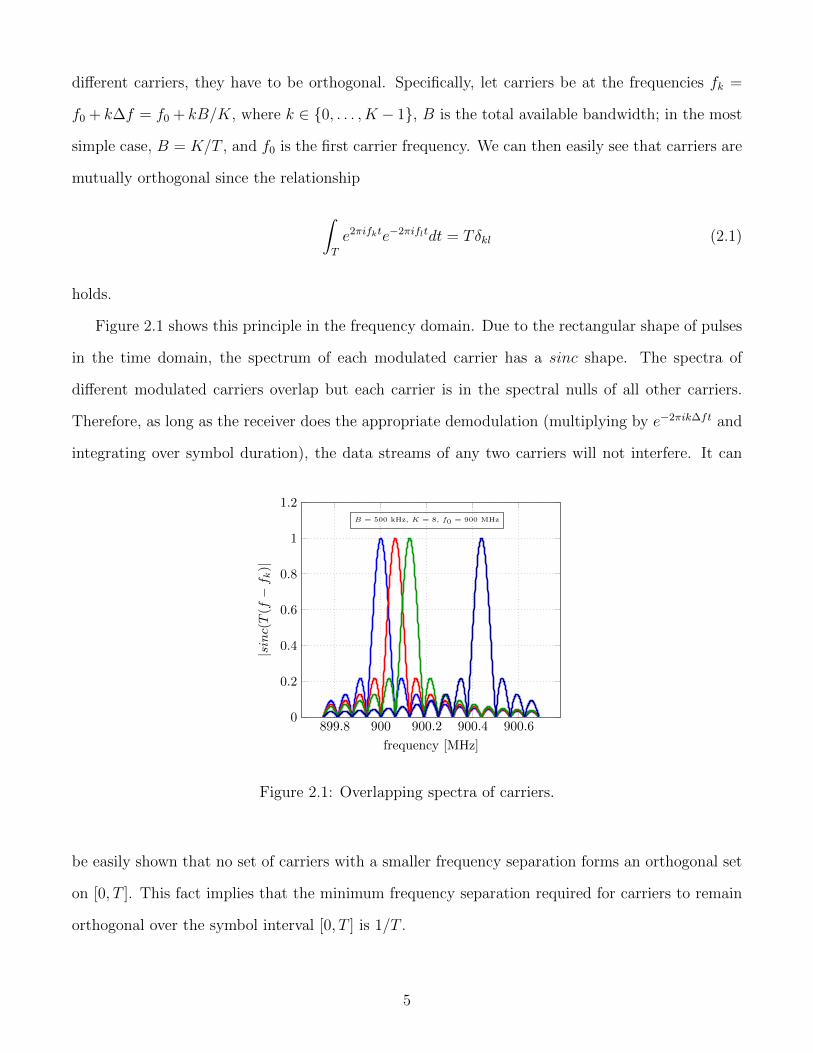
different carriers, they have to be orthogonal. Specifically, let carriers be at the frequencies fk =

f0 + k∆f = f0 + kB/K, where k ∈ {0, . . . , K − 1}, B is the total available bandwidth; in the most

simple case, B = K/T , and f0 is the first carrier frequency. We can then easily see that carriers are

mutually orthogonal since the relationship

∫T

e2πifkte−2πifltdt = Tδkl (2.1)

holds.

Figure 2.1 shows this principle in the frequency domain. Due to the rectangular shape of pulses

in the time domain, the spectrum of each modulated carrier has a sinc shape. The spectra of

different modulated carriers overlap but each carrier is in the spectral nulls of all other carriers.

Therefore, as long as the receiver does the appropriate demodulation (multiplying by e−2πik∆ft and

integrating over symbol duration), the data streams of any two carriers will not interfere. It can

899.8 900 900.2 900.4 900.60

0.2

0.4

0.6

0.8

1

1.2B = 500 kHz, K = 8, f0 = 900 MHz

frequency [MHz]

|sinc(T(f−

f k)|

Figure 2.1: Overlapping spectra of carriers.

be easily shown that no set of carriers with a smaller frequency separation forms an orthogonal set

on [0, T ]. This fact implies that the minimum frequency separation required for carriers to remain

orthogonal over the symbol interval [0, T ] is 1/T .

5

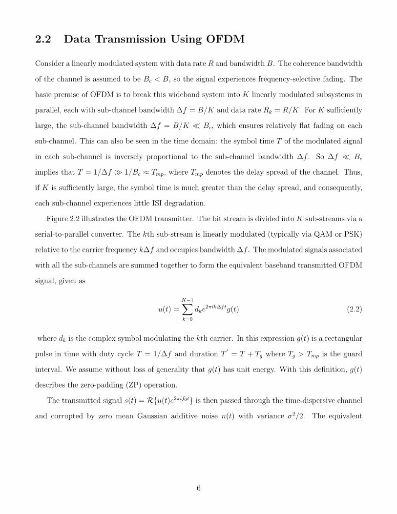
2.2 Data Transmission Using OFDM

Consider a linearly modulated system with data rate R and bandwidth B. The coherence bandwidth

of the channel is assumed to be Bc < B, so the signal experiences frequency-selective fading. The

basic premise of OFDM is to break this wideband system into K linearly modulated subsystems in

parallel, each with sub-channel bandwidth ∆f = B/K and data rate Rk = R/K. For K sufficiently

large, the sub-channel bandwidth ∆f = B/K � Bc, which ensures relatively flat fading on each

sub-channel. This can also be seen in the time domain: the symbol time T of the modulated signal

in each sub-channel is inversely proportional to the sub-channel bandwidth ∆f . So ∆f � Bc

implies that T = 1/∆f � 1/Bc ≈ Tmp, where Tmp denotes the delay spread of the channel. Thus,

if K is sufficiently large, the symbol time is much greater than the delay spread, and consequently,

each sub-channel experiences little ISI degradation.

Figure 2.2 illustrates the OFDM transmitter. The bit stream is divided into K sub-streams via a

serial-to-parallel converter. The kth sub-stream is linearly modulated (typically via QAM or PSK)

relative to the carrier frequency k∆f and occupies bandwidth ∆f . The modulated signals associated

with all the sub-channels are summed together to form the equivalent baseband transmitted OFDM

signal, given as

u(t) =K−1∑k=0

dke2πik∆ftg(t) (2.2)

where dk is the complex symbol modulating the kth carrier. In this expression g(t) is a rectangular

pulse in time with duty cycle T = 1/∆f and duration T′

= T + Tg where Tg > Tmp is the guard

interval. We assume without loss of generality that g(t) has unit energy. With this definition, g(t)

describes the zero-padding (ZP) operation.

The transmitted signal s(t) = R{u(t)e2πif0t} is then passed through the time-dispersive channel

and corrupted by zero mean Gaussian additive noise n(t) with variance σ2/2. The equivalent

6

serialto

parallel(S/P)

R [bps]

symbolmapper

RK [bps]

symbolmapper

RK [bps]

...

×d0

e2πi0∆ft

×dK−1

e2πi(K−1)∆ft

...Σ ×

g(t)

×

e2πif0t

u(t)R{.}

s(t)

Figure 2.2: OFDM Transmitter.

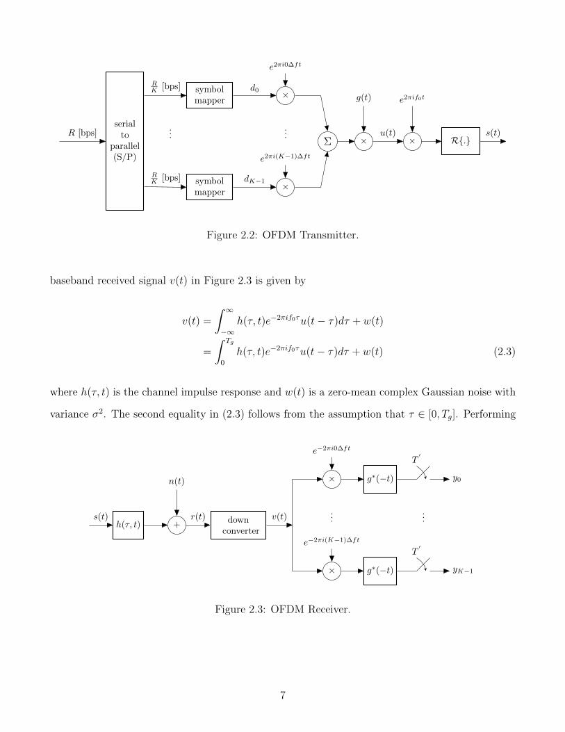
baseband received signal v(t) in Figure 2.3 is given by

v(t) =

∫ ∞−∞

h(τ, t)e−2πif0τu(t− τ)dτ + w(t)

=

∫ Tg

0

h(τ, t)e−2πif0τu(t− τ)dτ + w(t) (2.3)

where h(τ, t) is the channel impulse response and w(t) is a zero-mean complex Gaussian noise with

variance σ2. The second equality in (2.3) follows from the assumption that τ ∈ [0, Tg]. Performing

h(τ, t)s(t)

+

n(t)

downconverter

r(t) v(t)

×

e−2πi0∆ft

×

e−2πi(K−1)∆ft

...

g∗(−t)

g∗(−t)

T′

T′

...

y0

yK−1

Figure 2.3: OFDM Receiver.

7

ZP-OFDM demodulation, we obtain the output on the kth carrier as follows

yk =

∫ T′

0

v(t)e−2πik∆ftg(t)dt

=

∫ T′

0

(∫ Tg

0

h(τ, t)e−2πif0τ

K−1∑l=0

dle2πil∆f(t−τ)g(t− τ)dτ + w(t)

)e−2πik∆ftg(t)dt (2.4)

Assuming that the channel is not time-varying over each OFDM block, i.e., h(τ, t) = h(τ), t ∈

[0, T′], we have

yk =K−1∑l=0

dl

∫ T′

0

(∫ Tg

0

h(τ)e−2πi(f0+l∆f)τg(t− τ)dτ

)e2πi(k−l)∆ftg(t)dt+

∫ T′

0

w(t)e−2πik∆ftg(t)dt

(a)=

1

T

K−1∑l=0

dl

∫ T

0

(∫ Tg

0

h(τ)e−2πiflτdτ

)e2πi(k−l)∆ftdt+ zk

(b)=

K−1∑l=0

dlHlδlk + zk

= dkHk + zk (2.5)

where fl = f0+l∆f , Hk =∫ Tg

0h(τ)e−2πifkτdτ is the sampled channel frequency response at frequency

fk = f0 + k∆f and zk is a complex Gaussian random variable with zero mean and variance σ2z =

σ2. The equality (a) immediately follows from the definition of g(t) and the fact that the guard

interval must be less than the OFDM symbol interval in order for carriers to experience flat-fading

channels. The equality (b) stems from the orthonormality property of carriers in interval [0, T ]. The

expression (2.5) describes an OFDM system in the frequency domain and accentuates the fact that

the OFDM system effectively decomposes the wideband channel into a set of narrowband orthogonal

sub-channels with a different symbol sent over each sub-channel. Defining a stacked received vector

y, data matrix D, and noise vector z across all carriers, we can write the following input-output

relationship:

y = DH + z (2.6)

where D = diag(d0, d1, . . . , dK−1) and H is the channel vector with its kth entry given by Hk =∫ Tg0h(τ)e−2πifkτdτ . The noise vector z is a complex Gaussian random vector with zero mean and

8

covariance matrix σ2zI. In the next chapter, we extensively use this relationship to estimate the

channel vector H from the observation y, given the transmitted symbols D.

9

Chapter 3

Channel Estimation

Channel estimation is an indispensable part of a coherent OFDM system. With channel estimation,

OFDM systems can use coherent detection to obtain a 3 dB signal-to-noise ratio (SNR) gain over

differential detection. For OFDM systems with multiple transmit and/or receive antennas for sys-

tem capacity or performance improvement, channel information is essential to diversity combining,

interference suppression, and signal detection. In summary, the accuracy of channel state infor-

mation greatly influences the overall system performance. Therefore, in this chapter, we present

channel parameter estimation in OFDM systems.

In Section 3.1, we first introduce the physical, path-based channel model as an alternative to the

conventional discrete-delay (sample-spaced) channel model. Based on these two channel models, we

categorize the channel estimators into the discrete-delay (tap-based) channel estimators discussed

in Section 3.2 and path-based channel estimators which are investigated in Section 3.3.

3.1 Physical Channel and Discrete-Delay Models

To tackle the challenging problem of channel estimation, we firstly need to model the channel.

We propose two channel models; namely, path-based and discrete-delay (sample-spaced) channel

models. In the former model, we assume that a channel is composed of a number of physical paths

each of which is parameterized by a pair of path amplitude and path delay, (hp, τp). Hence, we can

10

write the channel impulse response as

h(τ) =∑p

hpδ(τ − τp) (3.1)

where the path delays τp have a continuum of values, i.e., they are not discrete and the path

amplitude hp is modeled as a complex zero-mean Gaussian random variable whose variance is a

function of e−τp . At the carrier frequencies fk = f0 + k∆f , we have

Hk = H(fk) =∑p

hpe−2πifkτp =

∑p

cpe−2πik∆fτp (3.2)

where cp = hpe−2πif0τp .

A baseband discrete-delay model with delay spacing ∆τ is given by

Hk =∑l

ble−2πik∆fl∆τ (3.3)

where bl’s are the channel taps. If we choose ∆τ = T/K and T = 1/∆f , then (3.3) becomes the

conventional DFT relationship,

H = FKb (3.4)

where H is the channel vector which appeared in (2.6) and FK is a K-point DFT matrix. In this

expression, b is the channel tap vector with its lth entry given by

bl =1

K

∑p

hpe−2πif0τpe−πi(K−1)(

τpT− lK

) sin(πK( τp

T− l

K))

sin(π( τp

T− l

K)) (3.5)

From (3.5), we can see that if the channel path delay τp is not an integer multiple of the delay

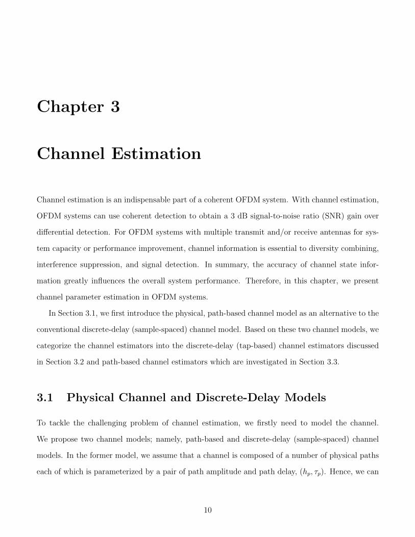
spacing, then the channel path amplitude hp will leak to all the taps, bl. Figure 3.1 illustrates this

leakage for a special case of a two-path equal-amplitude channel. We also observe that the most

significant taps are those in the neighborhood of the original impulse location.

11

0 10 20 30 40 50 60

0

0.2

0.4

0.6

tap number, l

|b l|

Figure 3.1: Spillage between taps for the physical channel h(τ) = δ(τ − 0.5 TK

) + δ(τ − 7.5 TK

).

3.2 Channel Estimation Based on the Discrete-Delay

Channel Model

3.2.1 Linear Minimum Mean Square Error (LMMSE) and Least

Squares (LS) Channel Estimators

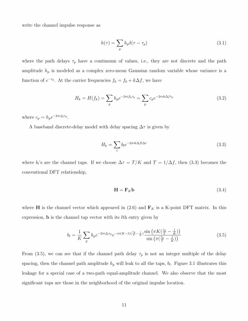
We will derive several estimators presented in [5, 11, 12]. These estimation techniques have the

general structure depicted in Figure 3.2. Based on the OFDM system model discussed in the

previous chapter and the discrete-delay channel model, we have

y = DFKb + z (3.6)

where the noise vector z ∼ CN (0, σ2zI) is uncorrelated with the channel taps. If we assume without

loss of generality that the receiver knows the data symbols D (training data symbols or decided

data symbols in the decision-directed-mode channel estimation), then we can obtain the linear-

minimum-mean-squared-error (LMMSE) estimate of channel taps as

blmmse = RbyR−1yy y (3.7)

12

frquency time frequency

IDFT

×

×

y0

d∗0

...

yK−1

d∗K−1

TDFT

H0

HK−1

Figure 3.2: General structure of the LS and LMMSE estimators.

where Rby = RbbFHKDH and Ryy = DFKRbbF

HKDH + σ2

zI are the cross-covariance matrix between

b and y and the auto-covariance matrix of y, respectively. The channel tap auto-covariance matrix

Rbb is assumed to be a-priori known which rarely happens in practice. Because of the orthonormal

property of the K-point Fourier matrix we also have

Hlmmse = FKblmmse

= FK Rbb

(Rbb + σ2

z

(FHKDHDFK

)−1)−1 (

FHKDHDFK

)−1︸ ︷︷ ︸Tlmmse

FHK

(DHy

)(3.8)

The conventional least-squares (LS) estimator for b minimizes ‖y −DFKb‖22 and generates

Hls = FK

(FHKDHDFK

)−1︸ ︷︷ ︸Tls

FHK

(DHy

)= D−1y (3.9)

Figure 3.3, which results from simulating an OFDM system with parameters shown in Table 3.1,

compares the performances of LMMSE and LS estimators in terms of normalized mean-squares error

NMSE , 1KE{‖H − H‖2

2} and computation time. We use 50000 realizations of the channel to

obtain the sample correlation matrix Rbb. The LMMSE estimator outperforms the LS estimator

but it requires more computations.

13

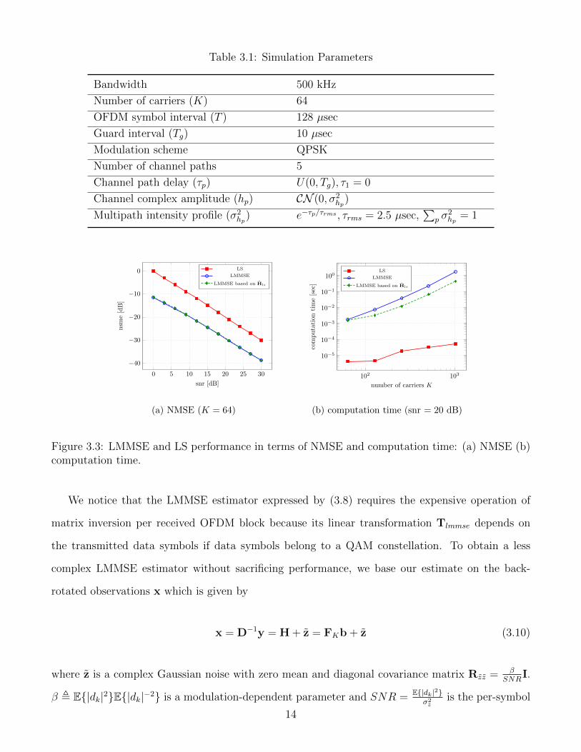
Table 3.1: Simulation Parameters

Bandwidth 500 kHz

Number of carriers (K) 64

OFDM symbol interval (T ) 128 µsec

Guard interval (Tg) 10 µsec

Modulation scheme QPSK

Number of channel paths 5

Channel path delay (τp) U(0, Tg), τ1 = 0

Channel complex amplitude (hp) CN (0, σ2hp

)

Multipath intensity profile (σ2hp

) e−τp/τrms , τrms = 2.5 µsec,∑

p σ2hp

= 1

0 5 10 15 20 25 30

−40

−30

−20

−10

0

snr [dB]

nsm

e[dB]

LS

LMMSE

LMMSE based on Hls

(a) NMSE (K = 64)

102 103

10−5

10−4

10−3

10−2

10−1

100

number of carriers K

computation

time[sec]

LS

LMMSE

LMMSE based on Hls

(b) computation time (snr = 20 dB)

Figure 3.3: LMMSE and LS performance in terms of NMSE and computation time: (a) NMSE (b)computation time.

We notice that the LMMSE estimator expressed by (3.8) requires the expensive operation of

matrix inversion per received OFDM block because its linear transformation Tlmmse depends on

the transmitted data symbols if data symbols belong to a QAM constellation. To obtain a less

complex LMMSE estimator without sacrificing performance, we base our estimate on the back-

rotated observations x which is given by

x = D−1y = H + z = FKb + z (3.10)

where z is a complex Gaussian noise with zero mean and diagonal covariance matrix Rzz = βSNR

I.

β , E{|dk|2}E{|dk|−2} is a modulation-dependent parameter and SNR = E{|dk|2}σ2z

is the per-symbol

14

signal-to-noise ratio. Based on back-rotated observations x, the LMMSE estimate of H becomes

Hlmmse = FKRbb

(KRbb +

β

SNRI

)−1

FHKx (3.11)

= RHH

(RHH +

β

SNRI

)−1

x (3.12)

where RHH = FKRbbFHK is the covariance matrix of the channel vector H. The explicit expression

for the NMSE of this estimator is given by

NMSElmmse =1

Ktrace

(E{(

H− Hlmmse

)(H− Hlmmse

)H})=

1

K

β

SNR

K−1∑k=0

Kλk

Kλk + βSNR

(3.13)

where λk’s are the eignevalues of Rbb. As Figure 3.3a illustrates, the difference between NMSE of

this estimator and the one expressed by (3.8) is negligible. However, as shown in Figure 3.3b, this

new LMMSE estimator needs less computation because, based on (3.11), its linear transformation

Tlmmse = Rbb

(KRbb + β

SNRI)−1

is data-independent.

Further reduction in complexity can be done by capitalizing on the fact that the multipath

spread Tmp is within LTK

. This essentially means that we can write

H = FKLbL (3.14)

where only the first L columns of the Fourier matrix FK and the first L elements of the channel tap

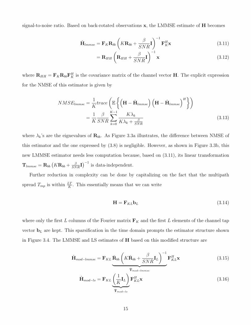
vector bL are kept. This sparsification in the time domain prompts the estimator structure shown

in Figure 3.4. The LMMSE and LS estimates of H based on this modified structure are

Hmod−lmmse = FKL Rbb

(KRbb +

β

SNRIL

)−1

︸ ︷︷ ︸Tmod−lmmse

FHKLx (3.15)

Hmod−ls = FKL

(1

KIL

)︸ ︷︷ ︸Tmod−ls

FHKLx (3.16)

15

frquency time frequency

IDFT

×Hls,0

×Hls,K−1

y0

d−10

...

yK−1

d−1K−1

T

bls,0

bls,L−1 DFT0

0

H0

HK−1

Figure 3.4: Modified structure.

where Rbb is the L × L auto-covariance matrix of bL and IL is an L × L identity matrix. These

modified estimators experience an error floor due to K − L excluded taps. The explicit expression

for the NMSE of these estimators are given by

NMSEmod−lmmse =1

K

β

SNR

L−1∑l=0

Kλl

Kλl + βSNR

+K−1∑l=L

σ2bl

(3.17)

NMSEmod−ls =L

K

β

SNR+

K−1∑l=L

σ2bl

(3.18)

where λl’s are the eignevalues of Rbb and σ2bl

is the lth channel tap power.

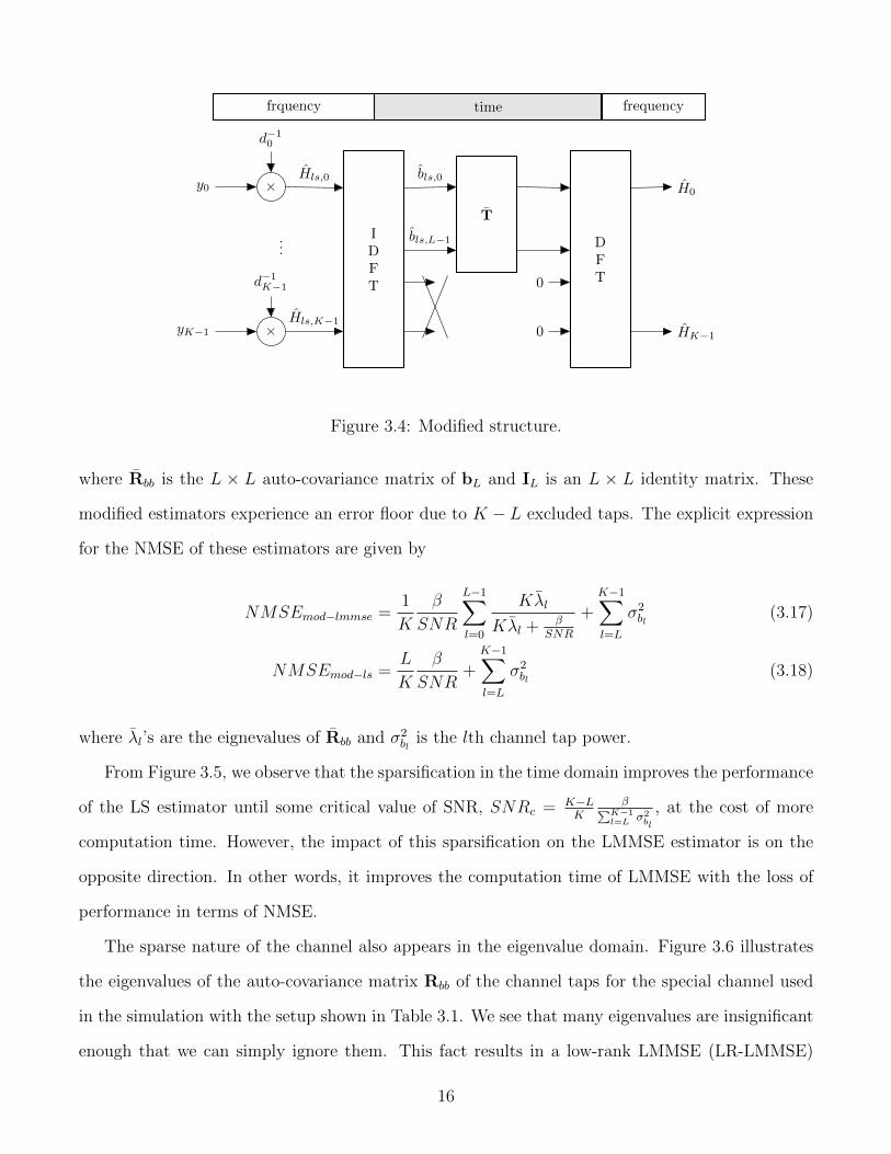
From Figure 3.5, we observe that the sparsification in the time domain improves the performance

of the LS estimator until some critical value of SNR, SNRc = K−LK

β∑K−1l=L σ2

bl

, at the cost of more

computation time. However, the impact of this sparsification on the LMMSE estimator is on the

opposite direction. In other words, it improves the computation time of LMMSE with the loss of

performance in terms of NMSE.

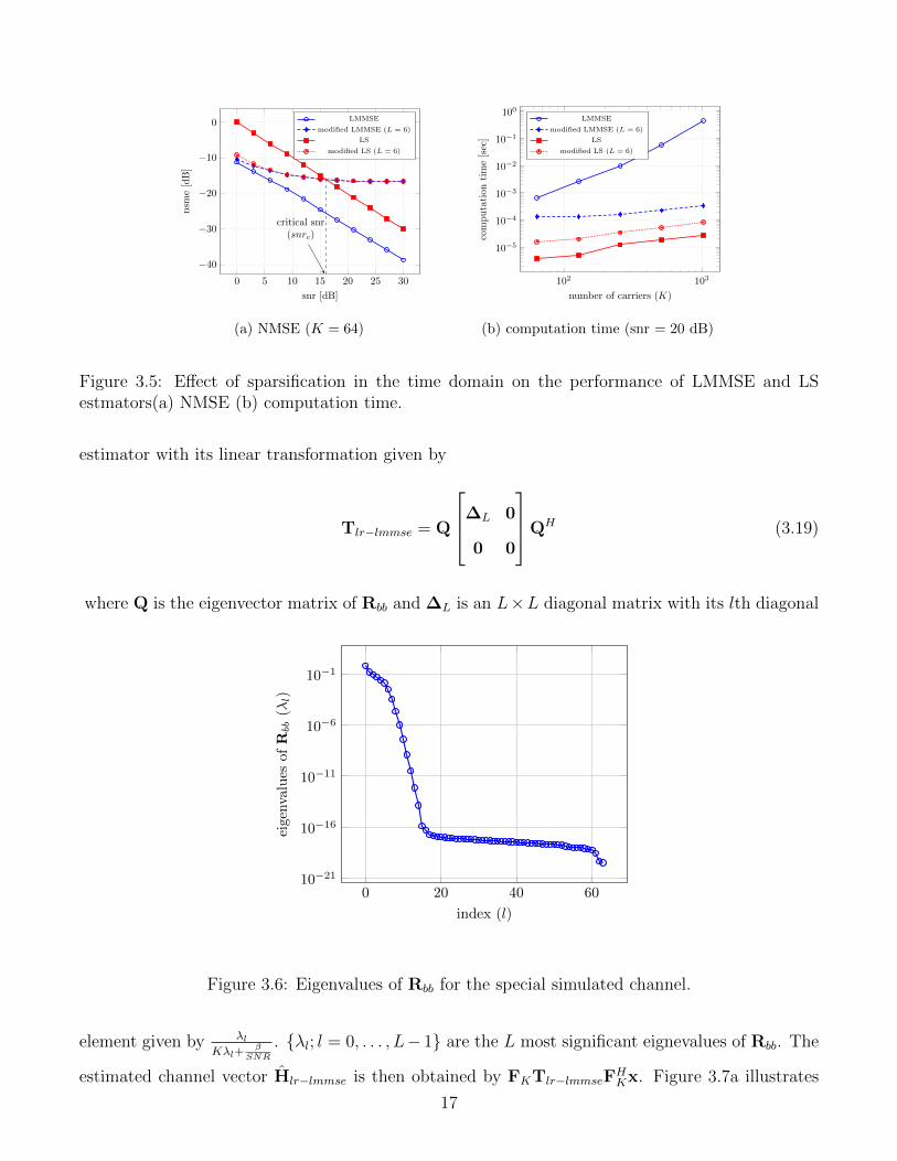
The sparse nature of the channel also appears in the eigenvalue domain. Figure 3.6 illustrates

the eigenvalues of the auto-covariance matrix Rbb of the channel taps for the special channel used

in the simulation with the setup shown in Table 3.1. We see that many eigenvalues are insignificant

enough that we can simply ignore them. This fact results in a low-rank LMMSE (LR-LMMSE)

16

0 5 10 15 20 25 30

−40

−30

−20

−10

0

critical snr(snrc)

snr [dB]

nsm

e[dB]

LMMSE

modified LMMSE (L = 6)

LS

modified LS (L = 6)

(a) NMSE (K = 64)

102 103

10−5

10−4

10−3

10−2

10−1

100

number of carriers (K)

computationtime[sec]

LMMSE

modified LMMSE (L = 6)

LS

modified LS (L = 6)

(b) computation time (snr = 20 dB)

Figure 3.5: Effect of sparsification in the time domain on the performance of LMMSE and LSestmators(a) NMSE (b) computation time.

estimator with its linear transformation given by

Tlr−lmmse = Q

∆L 0

0 0

QH (3.19)

where Q is the eigenvector matrix of Rbb and ∆L is an L×L diagonal matrix with its lth diagonal

0 20 40 6010−21

10−16

10−11

10−6

10−1

index (l)

eigenvalues

ofR

bb(λ

l)

Figure 3.6: Eigenvalues of Rbb for the special simulated channel.

element given by λlKλl+

βSNR

. {λl; l = 0, . . . , L− 1} are the L most significant eignevalues of Rbb. The

estimated channel vector Hlr−lmmse is then obtained by FKTlr−lmmseFHKx. Figure 3.7a illustrates

17

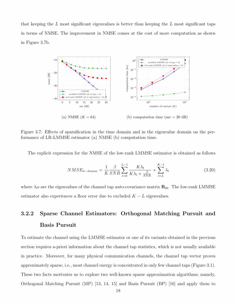
that keeping the L most significant eigenvalues is better than keeping the L most significant taps

in terms of NMSE. The improvement in NMSE comes at the cost of more computation as shown

in Figure 3.7b.

0 5 10 15 20 25 30

−40

−30

−20

−10

snr [dB]

nsm

e[dB]

LMMSE

modified LMMSE (# of taps = 6)

low-rank LMMSE (# of eigenvalues = 6)

(a) NMSE (K = 64)

102 103

10−4

10−3

10−2

10−1

100

number of carriers (K)

computationtime[sec]

LMMSE

modified LMMSE (# of taps = 6)

low-rank LMMSE (# of eignevalues = 6)

(b) computation time (snr = 20 dB)

Figure 3.7: Effects of sparsification in the time domain and in the eigenvalue domain on the per-formance of LR-LMMSE estimator (a) NMSE (b) computation time.

The explicit expression for the NMSE of the low-rank LMMSE estimator is obtained as follows

NMSElr−lmmse =1

K

β

SNR

L−1∑l=0

Kλl

Kλl + βSNR

+K−1∑l=L

λl (3.20)

where λls are the eigenvalues of the channel tap auto-covariance matrix Rbb. The low-rank LMMSE

estimator also experiences a floor error due to excluded K − L eigenvalues.

3.2.2 Sparse Channel Estimators: Orthogonal Matching Pursuit and

Basis Pursuit

To estimate the channel using the LMMSE estimator or one of its variants obtained in the previous

section requires a-priori information about the channel tap statistics, which is not usually available

in practice. Moreover, for many physical communication channels, the channel tap vector proves

approximately sparse, i.e., most channel energy is concentrated in only few channel taps (Figure 3.1).

These two facts motivates us to explore two well-known sparse approximation algorithms; namely,

Orthogonal Matching Pursuit (MP) [13, 14, 15] and Basis Pursuit (BP) [16] and apply them to

18

the channel estimation problem. These algorithms basically eliminate the need of knowledge about

the statistical characteristics of the channel and rely only on the sparse nature of the multipath

channels.

The channel model which we employ herein to present OMP and BP is a “super-resolution”

version of the model described in (3.3) with T = 1/∆f , ∆τ = T/IK where I ∈ Z+ accounts for

an increased resolution in the delay domain. By increasing the resolution factor I, the amount of

spillage between the taps decreases and sparsity of b becomes more conspicuous as illustrated in

Figure 3.8.

0 0.2 0.4 0.6 0.8 1 1.2

·10−4

0

0.2

0.4

0.6

delay (τ)

|b l|

I = 1

I = 2

Figure 3.8: Effect of the resolution factor I on the channel tap sparsity of the physical channelh(τ) = δ(τ − 0.5 T

K) + δ(τ − 7.5 T

K).

Based on the super-resolution discrete-delay channel model, the channel estimation problem

becomes the problem of identifying the approximately-sparse channel tap vector b in

x = Fb︸︷︷︸H

+z (3.21)

where the rows of the K × IK matrix F are the first K rows of a IK × IK DFT matrix and the

noise vector z ∼ CN (0, σ2zI) is uncorrelated with the channel taps. In compressive sensing literature,

when I > 1, the matrix F is called an overcomplete dictionary and its columns are called atom.

19

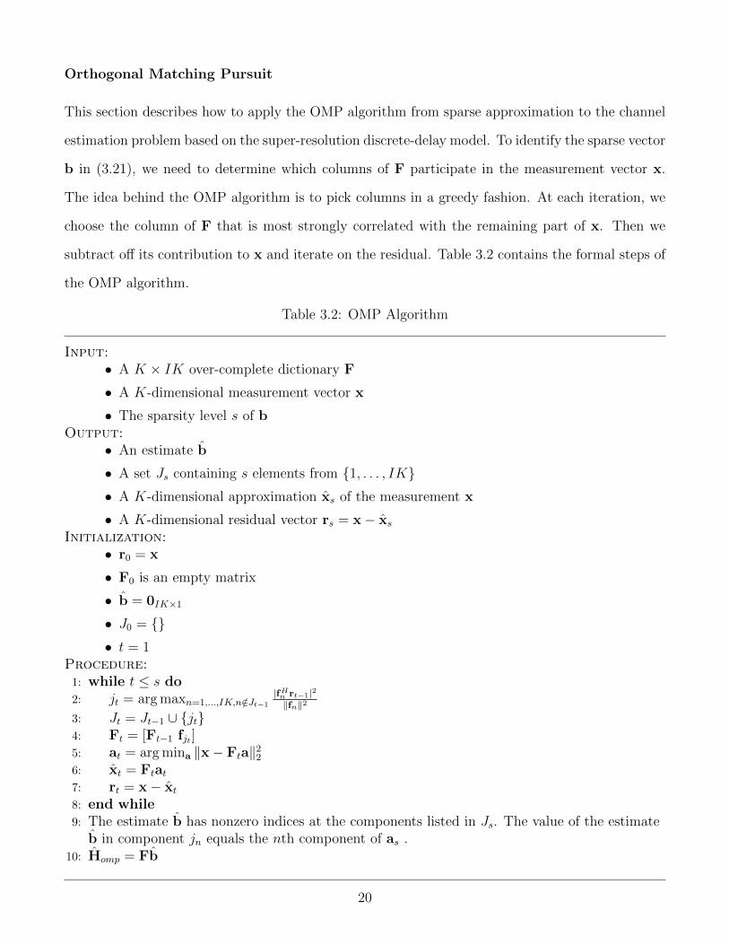
Orthogonal Matching Pursuit

This section describes how to apply the OMP algorithm from sparse approximation to the channel

estimation problem based on the super-resolution discrete-delay model. To identify the sparse vector

b in (3.21), we need to determine which columns of F participate in the measurement vector x.

The idea behind the OMP algorithm is to pick columns in a greedy fashion. At each iteration, we

choose the column of F that is most strongly correlated with the remaining part of x. Then we

subtract off its contribution to x and iterate on the residual. Table 3.2 contains the formal steps of

the OMP algorithm.

Table 3.2: OMP Algorithm

Input:• A K × IK over-complete dictionary F

• A K-dimensional measurement vector x

• The sparsity level s of bOutput:

• An estimate b

• A set Js containing s elements from {1, . . . , IK}• A K-dimensional approximation xs of the measurement x

• A K-dimensional residual vector rs = x− xsInitialization:

• r0 = x

• F0 is an empty matrix

• b = 0IK×1

• J0 = {}• t = 1

Procedure:1: while t ≤ s do2: jt = arg maxn=1,...,IK,n/∈Jt−1

|fHn rt−1|2‖fn‖2

3: Jt = Jt−1 ∪ {jt}4: Ft = [Ft−1 fjt ]5: at = arg mina ‖x− Fta‖2

2

6: xt = Ftat7: rt = x− xt8: end while9: The estimate b has nonzero indices at the components listed in Js. The value of the estimate

b in component jn equals the nth component of as .10: Homp = Fb

20

Steps 5, 6, 7, and 9 have been written to emphasize the conceptual structure of the OMP

algorithm; they can be implemented more efficiently. It is important to recognize that the residual

rt is always orthogonal to the columns of Ft. Provided that the residual rt−1 is non-zero, the

algorithm selects a new column at iteration m and the matrix Ft has full column rank. In which

case the solution at to the least squares problem in step 5 is unique. The running time of the OMP

algorithm is dominated by Step 2, whose total cost is O(sIK2). At iteration t, the least squares

problem can be solved with marginal cost O(tIK). To do so, we maintain a QR factorization of Ft.

Our implementation uses the Modified Gram-Schmidt (MGS) algorithm. The book [17] provides

extensive details and a survey of alternate approaches.

Since OMP is an iterative algorithm, we must supply a method for deciding when to halt the

iteration. There are three obvious possibilities:

(1) Stop the algorithm after a fixed number s of iterations.

(2) Wait until the norm of the residual declines to a level ε, i.e., ‖rt‖2 < ε.

(3) Halt the algorithm when the maximum total correlation between a column of F and the

residual drops below a threshold ξ, i.e., ‖FHrt‖∞ < ξ.

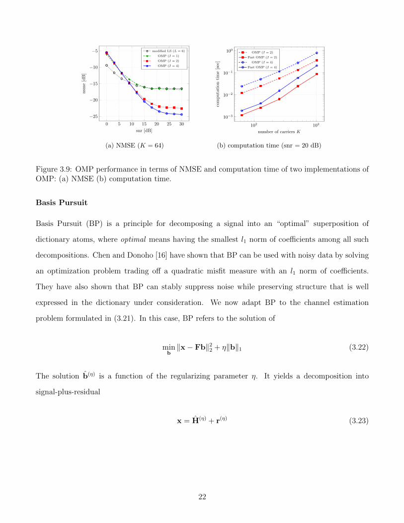
Figure 3.9a demonstrates the performance of the OMP algorithm for three different values of

the resolution factor I and compares their performance with the benchmark modified LS algorithm.

The simulation setup to obtain Figure 3.9 is the same as the setup in Table 3.1. In the simulation,

we use the number of path as the stopping criterion (first item in the list above). As shown

in Figure 3.9a, increasing the resolution factor improves the performance of the OMP. However,

the improvement in performance comes at increased computational complexity as illustrated in

Figure 3.9b. Furthermore, Figure 3.9a reveals that there is a strongly diminishing return for larger

resolution factor [6]. Figure 3.9b also compares the computation time of two implementations of

the OMP algorithm; namely, OMP and fast OMP. In the fast OMP implementation, we use the

MGS algorithm to solve the least squares problem in Step 5.

21

0 5 10 15 20 25 30

−25

−20

−15

−10

−5

snr [dB]

nsm

e[dB]

modified LS (L = 6)

OMP (I = 1)

OMP (I = 2)

OMP (I = 4)

(a) NMSE (K = 64)

102 103

10−3

10−2

10−1

100

number of carriers K

computationtime[sec]

OMP (I = 2)

Fast OMP (I = 2)

OMP (I = 4)

Fast OMP (I = 4)

(b) computation time (snr = 20 dB)

Figure 3.9: OMP performance in terms of NMSE and computation time of two implementations ofOMP: (a) NMSE (b) computation time.

Basis Pursuit

Basis Pursuit (BP) is a principle for decomposing a signal into an “optimal” superposition of

dictionary atoms, where optimal means having the smallest l1 norm of coefficients among all such

decompositions. Chen and Donoho [16] have shown that BP can be used with noisy data by solving

an optimization problem trading off a quadratic misfit measure with an l1 norm of coefficients.

They have also shown that BP can stably suppress noise while preserving structure that is well

expressed in the dictionary under consideration. We now adapt BP to the channel estimation

problem formulated in (3.21). In this case, BP refers to the solution of

minb‖x− Fb‖2

2 + η‖b‖1 (3.22)

The solution b(η) is a function of the regularizing parameter η. It yields a decomposition into

signal-plus-residual

x = H(η) + r(η) (3.23)

22

where H(η) = Hbp = Fb(η). Assuming the atoms of the dictionary F has unit norm, we set η to the

value

η = σz√

2 log card(F) (3.24)

where card(F) is the number of atoms in the dictionary F.

Figure 3.10 shows the performance of the Basis Pursuit technique in terms of NMSE and com-

putation time. This figure is the result of a simulation with parameters in Table 3.1. Figure 3.10a

illustrates that the BP technique outperforms the least squares method. This figure also accen-

tuates the facts that increasing the resolution in the sample-spaced delay domain improves the

BP performance and that there is a strongly diminishing return for finer dictionaries. According

0 5 10 15 20 25 30

−30

−20

−10

0

snr [dB]

nsm

e[dB]

LS

BP (I = 1)

BP (I = 2)

BP (I = 4)

(a) NMSE (K = 64)

101.8 102 102.2 102.4

10−0.4

10−0.2

100

100.2

100.4

number of carriers K

computation

time[sec]

BP (I = 1)

BP (I = 2)

BP (I = 4)

(b) computation time (snr = 20 dB)

Figure 3.10: BP performance in terms of NMSE and computation time: (a) NMSE (b) computationtime.

to [14, 18], there are algorithms that can solve BP in time O(I3/2K7/2). Figure 3.10b illustrates the

computation time of the BP algorithm using the CVX software package [19, 20] with the MOSEK

solver.

We show that using finer over-completer dictionaries improves the performance of both the

OMP and BP channel estimators because the dictionaries with higher delay resolution can explain

the channel with fewer non-zero taps. We also show that the improvement in the performance of

channel estimation saturates quickly.

23

3.3 Channel Estimation Based on the Physical Channel

Model

In this section, we focus on the physical, path-based channel model which is amenable to explicit

channel estimation, where the channel is parameterized by a number of distinct path, each character-

ized by a pair of complex amplitude and delay. We first relate the problem of channel estimation to

that of direction finding in the array processing literature. This relationship enables us to estimate

the path delays using the most widely-used array processing subspace method; namely, MUltiple

SIgnal Classification (MUSIC) [21, 22, 8, 9, 10, 23, 24]. Then, we propose our Path Identification

(PI) algorithm [25]. The PI algorithm is a greedy algorithm like the OMP algorithm and operates

in the continuous estimation space like MUSIC.

3.3.1 Relation between Direction Finding Problem and Channel Esti-

mation Problem

The problem of direction finding can be summarized as follows. Consider a uniform linear array

composed of K identical sensors. Let P < K narrowband plane waves, centered at frequency

f0, impinge on the array from directions {θ1, . . . , θP} relative to the broadside of the array. The

equivalent baseband received signal at the kth sensor can be expressed as

vk(t) =P∑p=1

up(t)e−2πif0(k−1) d

csin(θp) + wk(t) k = 1, . . . , K (3.25)

where up(t) is the signal of the pth wavefront, d is the spacing between the sensors, c is the propa-

gation speed of the wavefronts and wk(t) is the additive zero-mean complex Gaussian noise at the

kth sensor. The noises are assumed to be uncorrelated with the signals and uncorrelated between

themselves and to have identical variance σ2. Rewriting (3.25) in vector notation, we obtain

v(t) =

[a(θ1) · · · a(θP )

]︸ ︷︷ ︸

A

u(t) + w(t) (3.26)

24

where v(t) is a K × 1 array observation vector and a(θp) is the steering vector of the array in the

direction θp

a(θp) =

[1 e−2πif0

dc

sin(θp) · · · e−2πif0(K−1) dc

sin(θp)

]T(3.27)

In the direction finding problem, the P angles of arrival θp are unknown. We want to utilize the

array observation vector v(t) to estimate the signal subspace and utilize this information to estimate

the angles of arrival.

To make the link between the problem of direction finding and that of channel estimation, we

revisit the path-based channel model expressed in (3.2). Stacking the channel frequency responses

at carrier frequencies fk = f0 + k∆f for k = 0, . . . , K − 1, we obtain

H =∑p

hpe−2πif0τp︸ ︷︷ ︸cp

s(2π∆fτp) (3.28)

where hp and τp are the path complex amplitude and the path delay, respectively, and the K × 1

channel steering vector s(2π∆fτp) is given by

s(2π∆fτp) =

[1 e−2πi∆fτp · · · e−2πi(K−1)∆fτp

]T(3.29)

Assuming that the OFDM receiver operates in the decision-directed mode, the problem of channel

estimation based on the path-based model can be formulated as

x =

[s(2π∆fτ1) · · · s(2π∆fτP )

]︸ ︷︷ ︸

S

c + z (3.30)

where x is the noisy channel observation, c is a P × 1 vector of path complex amplitudes and

z ∼ CN (0, σ2zI) is the noise vector. In the sequel, for the sake of simplicity of notation, 2π∆fτp is

denoted by φp. We refer to φp as the path delay angle. In the channel estimation problem, both

the path delays τp (or equivalently the path delay angles φp) and path complex amplitudes cp need

to be estimated which makes the channel estimation problem be a non-linear estimation problem.

25

Problems expressed in (3.26) and (3.30) are mathematically identical if 2π∆fτp = 2πf0dc

sin(θp)

which makes a(θp) and s(φp) have the same Vandermonde structure1. Therefore, we can utilize the

direction finding methods to estimate the channel path delays. After finding the estimates of the

path delays angles estimates, φp, using one of the subspace algorithms presented in the next section,

we can obtain the estimates of the path complex amplitudes through

c = (SHS)−1SHx (3.31)

where S =

[s(φ1) · · · s(φP )

]and φp = 2π∆f τp.

3.3.2 Subspace Method: MUSIC

Subspace techniques have been advanced as a means of estimating the direction of arrivals of signals

incident on an array. The subspace methods hinge on the eigendecomposition of the correlation

matrix of the channel observation, x. From (3.30) it follows that

Rx = E{xxH} = SRcSH + σ2

zI (3.32)

where Rc = E{ccH} is the P × P correlation matrix of path amplitudes.

From the fact that channel path delays are different, it follows that the columns of the matrix

S are all different, and hence, because of their Vandermonde structure, linearly independent. In

addition, if the channel path amplitudes are uncorrelated or even partially correlated, then the

correlation matrix of channel path amplitudes Rc is non-singular and we have

rank(SRcSH) = P (3.33)

Let

{λ1 ≥ λ2 ≥ · · ·λP ≥ λP+1 ≥ · · · ≥ λK} and {q1,q2, . . .qP ,qP+1, . . . ,qK} (3.34)

1An m×n matrix A is called to have the Vandermonde structure if [A]i,j = αi−1j ,∀i = 1, . . . ,m and j = 1, . . . , n

where αj ∈ C, ∀j.

26

be the eigenvalues and the corresponding eigenvectors of Rx, then the rank property (3.33) implies

that

1. the minimal eigenvalue of Rx is equal to σ2z with multiplicity K − P

λP+1 = λP+2 = · · · = λK = σ2z (3.35)

2. the eigenvector corresponding to the minimal eigenvalue are orthogonal to the columns of the

matrix S; namely, to the steering vectors of the channel

{qP+1,qP+1, . . . ,qK} ⊥ {s(φ1), s(φ2), . . . , s(φP )} (3.36)

In array processing literature, the subspace spanned by the eigenvectors corresponding to the small-

est eigenvalue is referred to as the “noise” subspace. The orthogonal complement of the noise sub-

space is spanned by the steering vectors and is called the “signal” subspace. The theory of subspace

processing is based on the exploitation of (3.35) and (3.36). We first find the eigenvectors of Rx that

span the noise subspace QN =

[qP+1 · · · qK

]then project s(φ) onto QN for allowable values of

φ. The P values of φ where the projection is zero are the desired φ1, φ2, . . . , φP .

In practice, we do not know the correlation matrix Rx and must estimate it from the observation.

To estimate Rx, we need to observe a number of OFDM symbols to obtain the sample correlation

matrix Rx. Since we assume that the OFDM receiver operates in a block-by-block fashion, we

obtain the smoothed correlation matrix Rx based on one OFDM symbol only using the frequential

smoothing pre-processing scheme. Moreover, the number of channel paths P is rarely known in

practice. To estimate the number of channel paths, we use the widely-used Minimum Description

Length (MDL) source enumeration technique [26].

The Frequential Smoothing Pre-processing Scheme

We use the frequential smoothing pre-processing technique, introduced in [27, 28], to obtain the

smoothed correlation matrix which is structurally identical to the sample correlation matrix Rx, and

27

hence, we can successfully apply the eigenstructure method, MUSIC, to this smoothed correlation

matrix.

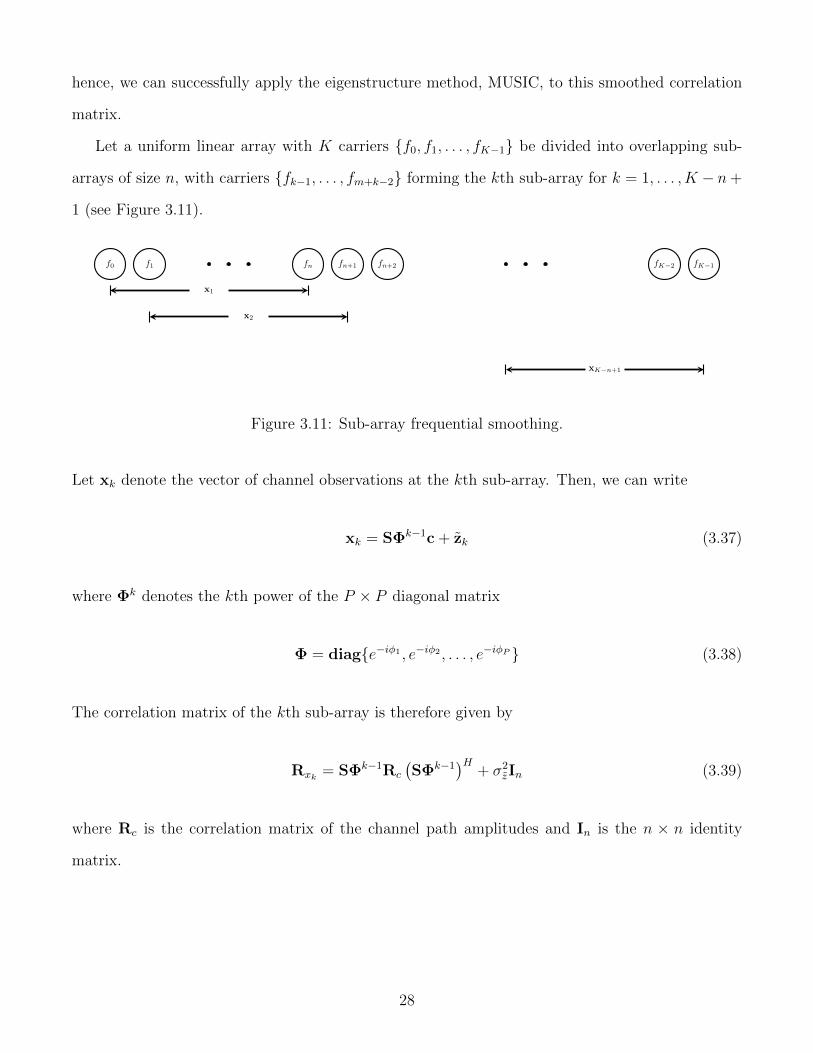
Let a uniform linear array with K carriers {f0, f1, . . . , fK−1} be divided into overlapping sub-

arrays of size n, with carriers {fk−1, . . . , fm+k−2} forming the kth sub-array for k = 1, . . . , K − n+

1 (see Figure 3.11).

f0 f1 fn fn+1 fn+2 fK−2 fK−1

x1

x2

xK−n+1

Figure 3.11: Sub-array frequential smoothing.

Let xk denote the vector of channel observations at the kth sub-array. Then, we can write

xk = SΦk−1c + zk (3.37)

where Φk denotes the kth power of the P × P diagonal matrix

Φ = diag{e−iφ1 , e−iφ2 , . . . , e−iφP } (3.38)

The correlation matrix of the kth sub-array is therefore given by

Rxk = SΦk−1Rc

(SΦk−1

)H+ σ2

zIn (3.39)

where Rc is the correlation matrix of the channel path amplitudes and In is the n × n identity

matrix.

28

The frequentially smoothed correlation matrix is defined as the sample mean of the sub-array

correlations

Rx =1

N

N∑k=1

Rxk (3.40)

where N = K − n+ 1 is the number of sub-arrays.

Using (3.39), we can rewrite (3.40) as

Rx = SRcSH + σ2

zIn (3.41)

where Rc is the modified correlation matrix of the channel path amplitudes, given by

Rc =1

N

N∑k=1

Φk−1Rc

(Φk−1

)H(3.42)

MUSIC

To estimate the path delays’ angles using the MUSIC algorithm [21], we first compute the null

spectrum given by

fmu(φ) = ‖s(φ)HQN‖22 = s(φ)HQNQH

Ns(φ) (3.43)

where the columns of QN are the eigenvectors of Rx corresponding to the minimal eigenvalue.

Determination of the estimates of the P path delay angles via the spectral MUSIC requires the

identification and accurate localization of multiple minima of the 1-d null spectrum, i.e., a nonlinear

search over a 1-d multimodal surface. Since the carriers in an OFDM system form an equispaced

array, we can use a polynomial representation. The steering polynomial vector is defined as

s(z) =

[1 z · · · zK−1

]T(3.44)

29

where z = e−iφ. Then (3.43) can be written as

fmu(z) = sTz (1

z)QNQH

Nsz(z) (3.45)

where fmu,z(z) is the conventional root-MUSIC polynomial [22]. We can simply show that the P

roots of fmu(z) on the unit circle correspond to the location in φ-space of the P channel paths. In

practice, we compute the roots of fmu(z) and choose the P roots that are inside the unit circle and

closest to the unit circle. Let zp, p = 1, 2, . . . , P denote these roots, then we have

φp = − arg zp, p = 1, . . . , P (3.46)

For a uniform linear array, the performance of the root-MUSIC algorithm can be improved by

using Forward-Backward (FB) averaging of the array observation to obtain the sample correlation

matrix

Rx,fb =1

2

(Rx + JR∗xJ

)(3.47)

where J is the exchange matrix with ones on its anti-diagonal and zeros elsewhere, and (.)∗ stands

for complex conjugate. The FB root-MUSIC polynomial is given by

fmu,fb(z) = sT (1

z)QN,fbQ

HN,fbs(z) (3.48)

The forward-backward root-MUSIC can be implemented with real computation by using a unitary

transformation. This approach is due to [23] and is called unitary root-MUSIC.

We define a real-valued sample correlation matrix as

Rx,re = UHRx,fbU (3.49)

30

where U can be any unitary, column conjugate symmetric matrix, i.e., JU∗ = U. For example, the

following sparse matrices

U =1√2

I iI

J −iJ

and U =1√2

I 0 iI

0T√

2 0T

J 0 −iJ

(3.50)

can be chosen for arrays with an even and odd number of array elements, respectively, where 0 =[0 0 · · · 0

]T. Interestingly, the matrix (3.49) can also be obtained via

Rx,re =1

2

(UHRxU + UHJRxJU

)=

1

2

(UHRxU + (U∗)H R∗xU

∗)

= R{UHRxU

}(3.51)

where R{z} denotes the real part of z.

The FB root-MUSIC polynomial in (3.48) can be written as

fmu,fb(z) = sT (1

z)UUHQN,fbQ

HN,fbUUHs(z)

(a)= sT (

1

z)UQN,reQ

TN,reU

Hs(z)

= sT (1

z)QN,reQ

TN,res(z) = fmu,u(z) (3.52)

0 5 10 15 20 25 30

−30

−25

−20

−15

−10

−5

snr [dB]

nsm

e[dB]

root-MUSIC

FB root-MUSIC

unitary root-MUSIC

unitary root-MUSIC with MDL

(a) NMSE (K = 64)

102 10310−3

10−2

10−1

100

101

number of carriers K

computation

time[sec]

FB root-MUSIC

unitary root-MUSIC

(b) computation time (snr = 20 dB)

Figure 3.12: MUSIC performance in terms of NMSE and computation time: (a) NMSE (b) com-putation time.

31

where the equality (a) follows from the facts that qre = UH qfb and λRx,re= λRx,fb

, s(z) = UHs(z)

and fmu,u(z) is the unitary root-MUSIC polynomial.

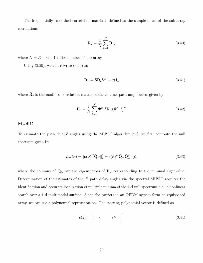
Using the same simulation parameters as shown in Table 3.1, Figure 3.12 illustrates the per-

formances of different versions of the MUSIC algorithm. We use sub-arrays with K/2 carrier to

perform the frequential smoothing pre-processing scheme. As shown in Figure 3.12b, the advantage

of unitary root-MUSIC is that it provides a significant reduction in computational complexity while

it has the same performance as FB root-MUSIC as illustrated in Figure 3.12a. In order to achieve

this reduction, we use an efficient root-finding algorithm developed by Lang and Frensel [29]. Fig-

ure 3.12a also shows the performance of the unitary root-MUSIC in which the number of channel

paths is estimated by the MDL technique.

3.3.3 Path Identification (PI) Algorithm

In this section, we propose our Path Identification (PI)algorithm [25]. The PI algorithm focuses

on explicit estimation of delays and complex amplitudes of the channel paths and is based on the

physical, path-based channel model

H =∑p

cps(φp) , φp = 2π∆fτp (3.53)

where

s(φ) =

[1 e−iφ · · · e−i(K−1)φ

]T(3.54)

represents the steering vector corresponding to an angle φ.

Consider now the following steering operation performed on the noisy channel observation x:

r(φ) =1

KsH(φ)x =

1

KsH(φ)

(∑p

cps(φp) + z

)(3.55)

32

This newly formed signal can be expressed as

r(φ) =∑p

cpg(φ− φp) + n(φ) (3.56)

where

g(φ) =1

K

K−1∑k=0

eikφ (3.57)

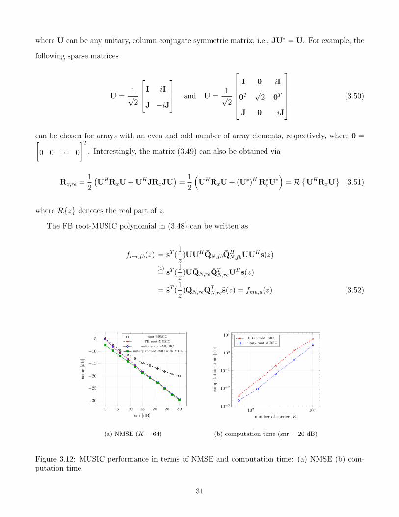
is the signature waveform and n(φ) is the complex Gaussian noise with variance 1Kσ2z . The signature

waveform (magnitude) is depicted in Figure 3.13. The fact that the signature waveform is known

can be exploited to estimate the channel parameters explicitly. When we say explicitly, we mean

that we are targeting directly both the path gains cp and the path delays τp (or more precisely the

angles φp), unlike in the conventional estimation where the delay axis is discretized to avoid the

non-linear problem of delay estimation.

−π −π2

0 π2

π0

0.2

0.4

0.6

0.8

1

1.2K = 64, ∆φ = 0.001π

φ

|g(φ)|

Figure 3.13: Signature waveform.

Joint estimation of the parameters cp and φp can be performed as follows. We start by setting

r1(φ) = r(φ) (3.58)

33

and evaluate this function for a pre-set range of angles φ with an arbitrary resolution ∆φ in the angle

domain. The range can be determined in accordance with the multipath spread Tmp. An iterative

procedure now follows over the path indices p = 1, . . . , P . In the p-th iteration, we estimate φp as

φp = arg maxφ|rp(φ)| (3.59)

and the path coefficient as

cp = rp(φ) (3.60)

We then subtract this path’s contribution from the current signal, so as to form the signal for the

next iteration

rp+1(φ) = rp(φ)− cpg(φ− φp) (3.61)

The procedure ends according to a pre-defined criterion such as an a-priori set number of paths,

or when the power in the residual reaches a certain threshold or stops to change significantly.

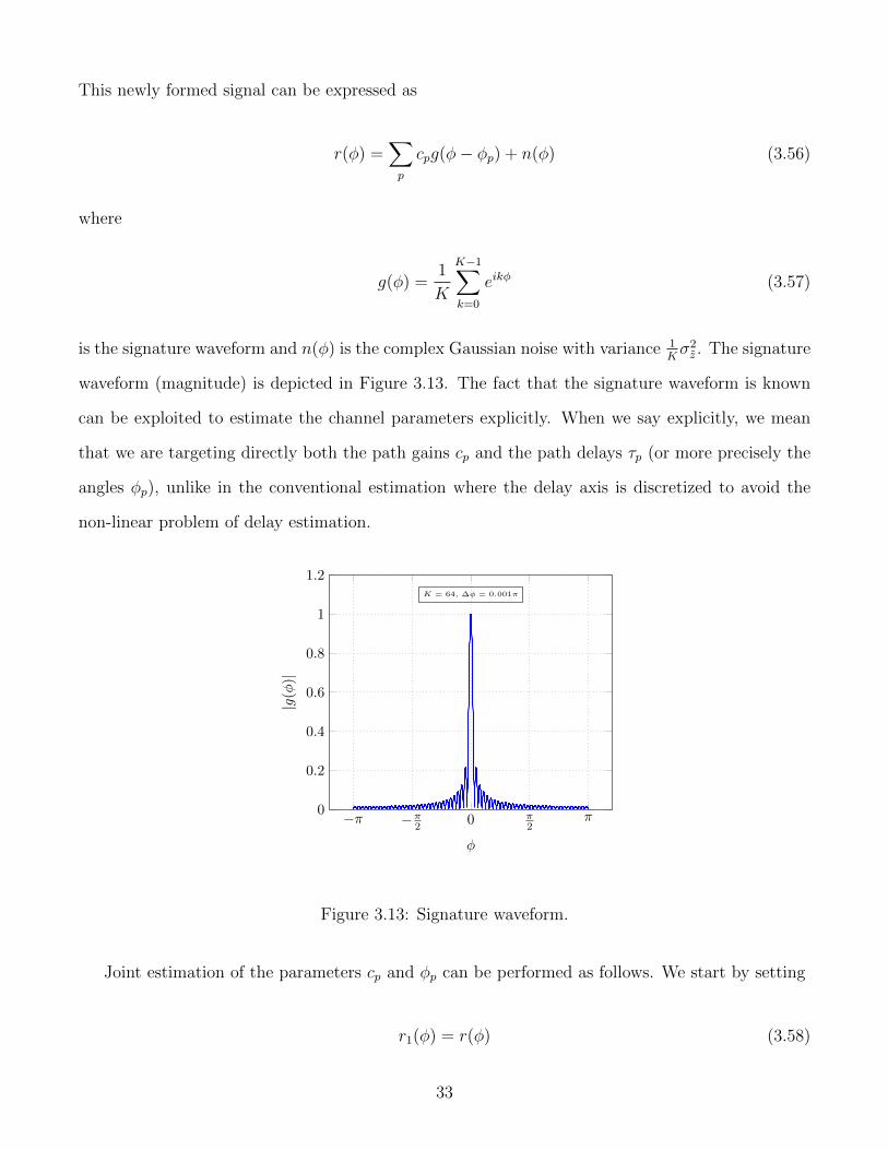
Figure 3.14 demonstrates the algorithm performance on one OFDM block with the SNR of 5 dB.

0 0.1 0.2 0.3 0.4 0.5

0

0.5

1

1.5

φ

|r(φ)|

(a) r(φ)

0 2 4 60

0.5

1

1.5

delay (τ) [µsec]

magnitude

true

PI estimates

(b) channel impulse response

0 15 31 47 63

1

2

3

carrier index (k)

magnitude

true

PI estimates

(c) channel frequency response

Figure 3.14: Demonstration of the PI algorithm applied to estimate the channel whose channelpath delays and amplitudes are hp = {1.25, 1.1, 0.95} and τp = {0, 2.125, 7.0625}, respectively: (a)magnitude of r(φ) (b) magnitude of channel impulse response (c) magnitude of channel frequencyresponse.

34

An extension to the above algorithm can also be applied to improve the quality of the estimates

cp. Once the algorithm has been executed, the path coefficients cp generated in the process are

discarded, but the angles φp are kept. The angles are used to form the matrix

S =

[s(φ1) · · · s(φP )

](3.62)

The channel coefficients are thus estimated as

c =(SHS

)−1

SHx (3.63)

Unlike with the estimates (3.59), which are obtained sequentially (one after another), these estimates

are obtained jointly, and hence offer a potential improvement. The PI algorithm is summarized in

Table 3.3.

Table 3.3: PI Algorithm

Input:• Channel observation x

• Number of channel paths (P ) (or a pre-defined threshold η)Output:

• Estimates φp, cpInitialization:

• r1(φ) = 1K

sH(φ)x

• p = 1Procedure:1: while p ≤ P (or 〈rp(φ), rp(φ)〉1 ≤ η) do

2: φp = arg maxφ |rp(φ)|3: cp = r(φp)

4: rp+1(φ) = rp(φ)− cpg(φ− φp)5: end while6: S =

[s(φ1) · · · s(φP )

]7: c =

(SHS

)−1

SHx

1〈rp(φ), rp(φ)〉 ,∫rp(φ)r

∗p(φ)dφ

35

0 5 10 15 20 25 30

−30

−20

−10

snr [dB]

nsm

e[dB]

PI (∆φ = 2π/K)

PI (∆φ = π/K)

PI (∆φ = π/2K)

PI with LS (∆φ = π/2K)

(a) NMSE (K = 64)

102 103

10−3

10−2.5

number of carriers K

computationtime[sec]

PI (∆φ = 2π/K)

PI (∆φ = π/K)

PI (∆φ = π/2K)

PI with LS (∆φ = π/2K)

(b) computation time

Figure 3.15: PI performance in terms of NMSE and computation time: (a) NMSE(b) computationtime.

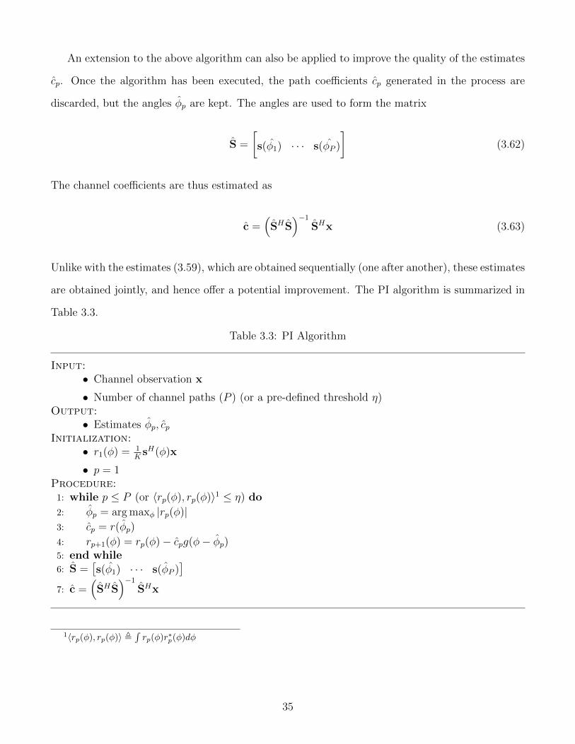
Figure 3.15 illustrates the performance of the PI algorithm for three different values of the

resolution ∆φ ∈ {2π/K, π/K, π/2K} which corresponds to the resolution factor I = {1, 2, 4}. We

use the simulation parameters shown in Table 3.1 and terminate the PI algorithm after 10 iterations.

As shown in Figure 3.15a, the performance of the PI algorithm does not saturate as quickly as the

tap-based channel estimators with over-complete dictionaries such as OMP and BP. This figure also

illustrates the fact that refining the estimates of cp in Step 7 improves the performance of the PI

algorithm without causing a significant increase in computation cost of the PI algorithm as depicted

in Figure 3.15b.

36

Chapter 4

Conclusion

We addressed the issue of channel estimation in OFDM systems, targeting explicitly the actual,

physical propagation paths, rather than the equivalent taps of a discrete-delay impulse response

model. The basic difference between the two approaches is that the former allows the path delays

to have a continuum of values, while the latter restricts the taps to a pre-defined quantization grid.

In pursuing the physical model, our goal was to reduce the total number of channel coefficients

(there are fewer paths than taps), and thus improve the system performance in the presence of

noise.

By employing a transformation of the signal received on a (large) number of OFDM carriers,

the channel estimation problem was cast into a framework where path delays and gains are to be

identified in a manner analogous to identifying angles of arrival in a typical beamforming (array

processing) framework. The major benefit of explicit tracking stems from the fact that its resolu-

tion in the delay domain can be increased arbitrarily, without a penalty on performance. Numerical

results indicate superiority of the proposed method over the standard sparse estimation techniques.

In Figure 4.1, we compare the performance of channel estimators in terms of NMSE and compu-

tation time. As must be obvious from Figure 4.1a, our proposed algorithm, Path Identification,

outperforms the modified LS, OMP, BP and unitary root-MUSIC. In terms of computation time,

the PI algorithm is more efficient than OMP, BP and unitary root-MUSIC.

37

0 5 10 15 20 25 30

−30

−20

−10

0

snr [dB]

nsm

e[dB]

PI with LS (∆φ = π/2K)

unitary root-MUSIC

modified LS (L = 6)

fast OMP (I = 4)

BP(I = 2)

(a) NMSE (K = 64)

102 10310−5

10−4

10−3

10−2

10−1

100

101

102

number of carriers K

computation

time[sec]

PI with LS (∆φ = π/2K)

unitary root-MUISC

modified LS (L = 6)

fast OMP (I = 4)

BP (I = 2)

(b) computation time

Figure 4.1: Performance of channel estimators: (a) NMSE(b) computation time.

38

Bibliography

[1] M. Salehi and J. Proakis, Digital Communications. McGraw-Hill Education, 2007.

[2] Y. G. Li and G. L. Stuber, Orthogonal frequency division multiplexing for wireless communi-cations. Springer Science & Business Media, 2006.

[3] O. Edfors, M. Sandell, J.-J. van de Beek, D. Landstrom, and F. Sjoberg, “An introduction toorthogonal frequency-division multiplexing,” Div. of Signal Processing, Research Report, 1996.

[4] B. Li, S. Zhou, M. Stojanovic, L. Freitag, and P. Willett, “Multicarrier communication overunderwater acoustic channels with nonuniform doppler shifts,” IEEE Journal of Oceanic En-gineering, vol. 33, no. 2, pp. 198–209, 2008.

[5] O. Edfors, M. Sandell, J.-J. Van De Beek, S. K. Wilson, and P. O. Borjesson, “OFDM channelestimation by singular value decomposition,” IEEE Transactions on Communications, vol. 46,no. 7, pp. 931–939, 1998.

[6] C. R. Berger, S. Zhou, J. C. Preisig, and P. Willett, “Sparse channel estimation for multicarrierunderwater acoustic communication: From subspace methods to compressed sensing,” IEEETransactions on Signal Processing, vol. 58, no. 3, pp. 1708–1721, 2010.

[7] C. R. Berger, Z. Wang, J. Huang, and S. Zhou, “Application of compressive sensing to sparsechannel estimation,” IEEE Communications Magazine, vol. 48, no. 11, pp. 164–174, 2010.

[8] T. Lo, J. Litva, and H. Leung, “A new approach for estimating indoor radio propagationcharacteristics,” IEEE Transactions on Antennas and Propagation, vol. 42, no. 10, pp. 1369–1376, 1994.

[9] S. E. Bensley and B. Aazhang, “Subspace-based channel estimation for code division multi-ple access communication systems,” IEEE Transactions on Communications, vol. 44, no. 8,pp. 1009–1020, 1996.

[10] B. H. Fleury, M. Tschudin, R. Heddergott, D. Dahlhaus, and K. I. Pedersen, “Channel pa-rameter estimation in mobile radio environments using the sage algorithm,” IEEE Journal onSelected Areas in Communications, vol. 17, no. 3, pp. 434–450, 1999.

[11] O. Edfors, M. Sandell, J.-J. Van De Beek, S. K. Wilson, and P. O. Borjesson, “Analysis ofDFT-based channel estimators for OFDM,” Wireless Personal Communications, vol. 12, no. 1,pp. 55–70, 2000.

[12] J.-J. Van de Beek, O. Edfors, M. Sandell, S. K. Wilson, and P. O. Borjesson, “On channelestimation in OFDM systems,” in Vehicular Technology Conference, 1995 IEEE 45th, vol. 2,pp. 815–819, IEEE, 1995.

39

[13] S. G. Mallat and Z. Zhang, “Matching pursuits with time-frequency dictionaries,” IEEE Trans-actions on Signal Processing, vol. 41, no. 12, pp. 3397–3415, 1993.

[14] J. A. Tropp and A. C. Gilbert, “Signal recovery from random measurements via orthogonalmatching pursuit,” IEEE Transactions on Information Theory, vol. 53, no. 12, pp. 4655–4666,2007.

[15] W. Li and J. C. Preisig, “Estimation of rapidly time-varying sparse channels,” IEEE Journalof Oceanic Engineering, vol. 32, no. 4, pp. 927–939, 2007.

[16] S. S. Chen, D. L. Donoho, and M. A. Saunders, “Atomic decomposition by basis pursuit,”SIAM review, vol. 43, no. 1, pp. 129–159, 2001.

[17] A. Bjorck, Numerical methods for least squares problems. Siam, 1996.

[18] Y. Nesterov and A. Nemirovskii, Interior-point polynomial algorithms in convex programming,vol. 13. SIAM, 1994.

[19] M. Grant and S. Boyd, “CVX: Matlab software for disciplined convex programming, version2.1.” http://cvxr.com/cvx, Mar. 2014.

[20] M. Grant and S. Boyd, “Graph implementations for nonsmooth convex programs,” in RecentAdvances in Learning and Control (V. Blondel, S. Boyd, and H. Kimura, eds.), Lecture Notesin Control and Information Sciences, pp. 95–110, Springer-Verlag Limited, 2008. http://

stanford.edu/~boyd/graph_dcp.html.

[21] R. Schmidt, “Multiple emitter location and signal parameter estimation,” IEEE Transactionson Antennas and Propagation, vol. 34, no. 3, pp. 276–280, 1986.

[22] B. D. Rao and K. Hari, “Performance analysis of root-MUSIC,” IEEE Transactions on Acous-tics, Speech, and Signal Processing, vol. 37, no. 12, pp. 1939–1949, 1989.

[23] M. Pesavento, A. B. Gershman, and M. Haardt, “Unitary root-MUSIC with a real-valuedeigendecomposition: A theoretical and experimental performance study,” IEEE Transactionson Signal Processing, vol. 48, no. 5, pp. 1306–1314, 2000.

[24] H. L. Van Trees, Detection, estimation, and modulation theory, optimum array processing.John Wiley & Sons, 2004.

[25] M. Stojanovic and S. Tadayon, “Estimation and tracking of time-varying channels in OFDMsystems,” in Communication, Control, and Computing (Allerton), 2014 52nd Annual AllertonConference on, pp. 116–122, IEEE, 2014.

[26] M. Wax and T. Kailath, “Detection of signals by information theoretic criteria,” IEEE Trans-actions on Acoustics, Speech, and Signal Processing, vol. 33, no. 2, pp. 387–392, 1985.

[27] T.-J. Shan, M. Wax, and T. Kailath, “On spatial smoothing for direction-of-arrival estimationof coherent signals,” IEEE Transactions on Acoustics, Speech, and Signal Processing, vol. 33,no. 4, pp. 806–811, 1985.

[28] S. U. Pillai and B. H. Kwon, “Forward/backward spatial smoothing techniques for coherentsignal identification,” IEEE Transactions on Acoustics, Speech, and Signal Processing, vol. 37,no. 1, pp. 8–15, 1989.

40

[29] M. Lang and B.-C. Frenzel, “Polynomial root finding,” IEEE Signal Processing Letters, vol. 1,no. 10, pp. 141–143, 1994.

41