CHANNEL ESTIMATION AND SYNCHRONIZATION FOR OFDM … · CHANNEL ESTIMATION AND SYNCHRONIZATION FOR OFDM SYSTEM ... (wireless) channel The ... choose the channel estimation technique

International Journal of Engineering Technology and Scientific Innovation

Volume:01,Issue:01

www.ijetsi.org

www.ijetsi.org Page 14

CHANNEL ESTIMATION AND SYNCHRONIZATION FOR

OFDM SYSTEM

Said Elkassimi1, Said Safi1

1Equipe de traitement de l’information et de télécommunications, facultés des sciences et Techniques,

USMS, Béni Mellal, Maroc

B.Manout2

2Laboratoire Interdisciplinaire de Recherche en Science et Technique (LIRST),

USMS Béni Mellal, Maroc

ABSTRACT

The OFDM system carries the message data on orthogonal subcarriers for parallel transmission,

combating the distortion caused by the frequency selective channel or equivalently, the inter-

symbol-interference in the multi-path fading channel. However, the advantage of the OFDM can

be useful only when the orthogonality is maintained, thus In an OFDM system, the transmitter

modulates the message bit sequence into PSK/QAM symbols, performs IFFT on the symbols to

convert them into time domain signals, and sends them out through a (wireless) channel The

received signal is usually distorted by the channel characteristics. In order to recover the

transmitted bits, the channel effect must be estimated and compensated in the receiver. First we

will discuss synchronization techniques to manage the STO and CFO potential problems in OFDM

systems, and the use of DFT technique for estimating the mobile radio channel response. Finally,

we simulate the synchronization technique STO, and LS-linear, LS-spline and MMSE with DFT

method for estimating the mobile radio channel parameters Bran A, thus a comparison of

performance of LS-linear, LS-spline and MMSE with DFT method.

Keywords: OFDM, STO, CFO, LS-linear, LS-spline, MMSE, DFT, BRAN A.

INTRODUCTION

The advantage of the OFDM can be useful

only when the orthogonality is maintained.

In case the orthogonality is not sufficiently

warranted by any means, its performance

may be degraded due to inter-symbol

interference (ISI) and inter-channel


Volume:01,Issue:01

www.ijetsi.org


interference (ICI) [1]. Thus, the transmitted

signal can be recovered by estimating the

channel response just at each subcarrier. In

general, the channel can be estimated by

using a preamble or pilot symbols known to

both transmitter and receiver, which employ

various interpolation techniques to estimate

the channel response of the subcarriers

between pilot tones. In general, data signal

as well as training signal, or both, can be

used for channel estimation. In order to

choose the channel estimation technique for

the OFDM system under consideration,

many different aspects of implementations,

including the required performance,

computational complexity and time-

variation of the channel must be taken into

account. In this article we discuss and

simulate the synchronization OFDM system

by STO technique, and the estimation

mobile radio channel response BRAN A [2]

by LS-linear, LS-spline and MMSE with

DFT method.

I. SYNCHRONISATION FOR OFDM

In this part, we will analyze the effects of

symbol time offset (STO) and carrier

frequencies offset (CFO), and then discuss

the synchronization techniques to handle the

potential STO and CFO problems in OFDM

systems. The received baseband signal under

the presence of CFO and STO can be

expressed as:

𝑦[𝑛] = 𝐼𝐷𝐹𝑇{𝑌[𝑛]}

= 𝐼𝐷𝐹𝑇{𝐻[𝑘]𝑋[𝑘] + 𝑍[𝑘]}

=1

𝑁∑𝐻[𝑘]𝑋[𝑘]𝑒𝑗2𝜋(𝑘+ )(𝑛+𝛿)𝑁

𝑁−1

𝑘=0

+ 𝑧[𝑛] (1)

Where 𝑧[𝑛] = 𝐼𝐷𝐹𝑇{𝑍[𝑘]} and 휀, 𝛿 the

normalized CFO and STO, respectively.

1. Estimation Techniques for STO

STO may cause not only phase distortion

(that can be compensated by using an

equalizer) but also ISI (that cannot be

corrected once occurred) in OFDM systems.

In order to warrant its performance,

therefore, the starting point of OFDM

symbols must be accurately determined by

estimating the STO with a synchronization

technique at the receiver. We discuss how to

estimate the STO. In general, STO

estimation can be implemented either in the

time or frequency domain.

1.1 Time-Domain Estimation Techniques

for STO

Consider an OFDM symbol with a cyclic

prefix (CP) of 𝑁𝐺 samples over 𝑇𝐺 seconds

and effective data of 𝑁𝑠𝑢𝑏 samples over

𝑇𝑠𝑢𝑏 seconds. In the time domain, STO can

be estimated by using CP or training

symbols. In the sequel, we discuss the STO

estimation techniques with CP or training

symbols.

a) STO Estimation Techniques Using

Cyclic Prefix (CP)

Recall that CP is a replica of the data part in

the OFDM symbol. It implies that CP and


Volume:01,Issue:01

www.ijetsi.org


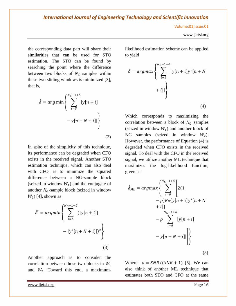
the corresponding data part will share their

similarities that can be used for STO

estimation. The STO can be found by

searching the point where the difference

between two blocks of 𝑁𝐺 samples within

these two sliding windows is minimized [3],

that is,

𝛿 = 𝑎𝑟𝑔min{ ∑ |𝑦[𝑛 + 𝑖]

𝑁𝐺−1+𝛿

𝑖=𝛿

− 𝑦[𝑛 + 𝑁 + 𝑖]|}

(2)

In spite of the simplicity of this technique,

its performance can be degraded when CFO

exists in the received signal. Another STO

estimation technique, which can also deal

with CFO, is to minimize the squared

difference between a NG-sample block

(seized in window 𝑊1) and the conjugate of

another 𝑁𝐺-sample block (seized in window

𝑊2) [4], shown as

𝛿 = 𝑎𝑟𝑔𝑚𝑖𝑛 { ∑ (|𝑦[𝑛 + 𝑖]|

𝑁𝐺−1+𝛿

𝑖=𝛿

− |𝑦∗[𝑛 + 𝑁 + 𝑖]|)2}

(3)

Another approach is to consider the

correlation between those two blocks in 𝑊1

and 𝑊2. Toward this end, a maximum-

likelihood estimation scheme can be applied

to yield

𝛿 = 𝑎𝑟𝑔𝑚𝑎𝑥 { ∑ |𝑦[𝑛 + 𝑖]𝑦∗[𝑛 + 𝑁

𝑁𝐺−1+𝛿

𝑖=𝛿

+ 𝑖]|}

(4)

Which corresponds to maximizing the

correlation between a block of 𝑁𝐺 samples

(seized in window 𝑊1) and another block of

NG samples (seized in window 𝑊2).

However, the performance of Equation (4) is

degraded when CFO exists in the received

signal. To deal with the CFO in the received

signal, we utilize another ML technique that

maximizes the log-likelihood function,

given as:

𝛿𝑀𝐿 = 𝑎𝑟𝑔𝑚𝑎𝑥 { ∑ [2(1

𝑁𝐺−1+𝛿

𝑖=𝛿

− 𝜌)𝑅𝑒{𝑦[𝑛 + 𝑖]𝑦∗[𝑛 + 𝑁

+ 𝑖]}

− 𝜌 ∑ |𝑦[𝑛 + 𝑖]

𝑁𝐺−1+𝛿

𝑖=𝛿

− 𝑦[𝑛 + 𝑁 + 𝑖]|]}

(5)

Where 𝜌 = 𝑆𝑁𝑅 (𝑆𝑁𝑅 + 1)⁄ [5]. We can

also think of another ML technique that

estimates both STO and CFO at the same


Volume:01,Issue:01

www.ijetsi.org


time as derived in [6]. In this technique, the

STO is estimated as:

𝛿𝑀𝐿 = 𝑎𝑟𝑔𝑚𝑎𝑥{|𝛾[𝛿]| − 𝜌𝜙[𝛿]} (6)

𝛾[𝑚] = ∑ 𝑦[𝑛]𝑦∗[𝑛 + 𝑁],

𝑚+𝐿−1

𝑛+𝑚

And

𝜙[𝑚] =1

2∑ {|𝑦[𝑛]|2

𝑚+𝐿−1

𝑛=𝑚

+ |𝑦[𝑛 + 𝑁]|2} (7)

Using 𝐿 to denote the actual number of

samples used for averaging in windows.

Taking the absolute value of the correlation

[𝑚] , STO estimation in Equation (6) can be

robust even under the presence of CFO.

b) STO Estimation Techniques Using

Training Symbol

Training symbols can be transmitted to be

used for symbol synchronization in the

receiver. In contrast with CP, it involves

overhead for transmitting training symbols,

but it does not suffer from the effect of the

multi-path channel. Once the transmitter

sends the repeated training signals over two

blocks within the OFDM symbol, the

receiver attempts to find the CFO by

maximizing the similarity between these two

blocks of samples received within two

sliding windows. The similarity between

two sample blocks can be computed by an

autocorrelation property of the repeated

training signal. As in the STO estimation

technique using CP, for example, STO can

be estimated by minimizing the squared

difference between two blocks of samples

received in 𝑊1 and 𝑊2 [7,8], such that

𝛿 = 𝑎𝑟𝑔𝑚𝑖𝑛

{

∑ |𝑦[𝑛 + 𝑖]

𝑁2−1+𝛿

𝑖=𝛿

− 𝑦∗ [𝑛 +𝑁

2+ 𝑖]|

2

}

(8)

Or by maximizing the likelihood function

[109], that is,

𝛿

= 𝑎𝑟𝑔𝑚𝑎𝑥

{

|∑ 𝑦[𝑛 + 𝑖]𝑦∗ [𝑛 +

𝑁2 + 𝑖]

𝑁2−1+𝛿

𝑖=𝛿|

2

|∑ 𝑦 [𝑛 +𝑁2 + 𝑖]

𝑁2−1+𝛿

𝑖=𝛿|

2

}

(9)

The difficulty in locating STO due to the flat

interval can be handled by taking the

average of correlation values over the length

of CP [103], shown as

𝛿 = 𝑎𝑟𝑔𝑚𝑎𝑥 (1

𝑁𝐺 + 1∑ 𝑠[𝑛 +𝑚]

𝑖

𝑚=−𝑁𝐺+𝑖

)

(10)

Where


Volume:01,Issue:01

www.ijetsi.org


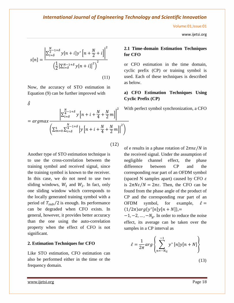
𝑠[𝑛] =

|∑ 𝑦[𝑛 + 𝑖]𝑦∗ [𝑛 +𝑁2 + 𝑖]

𝑁2−1+𝛿

𝑖=𝛿|

2

(12 |∑ 𝑦[𝑛 + 𝑖]𝑁−1+𝛿𝑖=𝛿 |

2)2

(11)

Now, the accuracy of STO estimation in

Equation (9) can be further improved with

𝛿

= 𝑎𝑟𝑔𝑚𝑎𝑥

|∑ 𝑦 [𝑛 + 𝑖 +𝑁4 +

𝑁2 𝑚]

𝑁4−1+𝛿

𝑖=𝛿|

2

(∑ ∑ |𝑦 [𝑛 + 𝑖 +𝑁4 +

𝑁2 𝑚]|

2𝑁4−1+𝛿

𝑖=𝛿1𝑚=0 )

(12)

Another type of STO estimation technique is

to use the cross-correlation between the

training symbol and received signal, since

the training symbol is known to the receiver.

In this case, we do not need to use two

sliding windows, 𝑊1 and 𝑊2. In fact, only

one sliding window which corresponds to

the locally generated training symbol with a

period of 𝑇𝑠𝑢𝑏 2⁄ is enough. Its performance

can be degraded when CFO exists. In

general, however, it provides better accuracy

than the one using the auto-correlation

property when the effect of CFO is not

significant.

2. Estimation Techniques for CFO

Like STO estimation, CFO estimation can

also be performed either in the time or the

frequency domain.

2.1 Time-domain Estimation Techniques

for CFO

or CFO estimation in the time domain,

cyclic prefix (CP) or training symbol is

used. Each of these techniques is described

as below.

a) CFO Estimation Techniques Using

Cyclic Prefix (CP)

With perfect symbol synchronization, a CFO

of e results in a phase rotation of 2𝜋𝑛휀 𝑁⁄ in

the received signal. Under the assumption of

negligible channel effect, the phase

difference between CP and the

corresponding rear part of an OFDM symbol

(spaced N samples apart) caused by CFO 휀

is 2𝜋𝑁휀 𝑁⁄ = 2𝜋휀. Then, the CFO can be

found from the phase angle of the product of

CP and the corresponding rear part of an

OFDM symbol, for example, 휀̂ =

(1 2𝜋⁄ )𝑎𝑟𝑔{𝑦∗[𝑛]𝑦[𝑛 + 𝑁]},=

−1,−2, … , −𝑁𝑔. In order to reduce the noise

effect, its average can be taken over the

samples in a CP interval as

휀̂ =1

2𝜋𝑎𝑟𝑔 { ∑ 𝑦∗

−1

𝑛=−𝑁𝐺

[𝑛]𝑦[𝑛 + 𝑁]}

(13)


Volume:01,Issue:01

www.ijetsi.org


Since the argument operation arg() is

performed by using tan-1(), the range of CFO

estimation in Equation (13) is [– 0.5, 0.5] so

that |휀̂| < 0.5 and consequently, integral

CFO cannot be estimated by this technique.

Note that 𝑦∗[𝑛]𝑦[𝑛 + 𝑁] becomes real only

when there is no frequency offset. This

implies that it becomes imaginary as long as

the CFO exists. In fact, the imaginary part of

𝑦∗[𝑛]𝑦[𝑛 + 𝑁] can be used for CFO

estimation [9]. In this case, the estimation

error is defined as:

𝑒 =1

𝐿∑ 𝐼𝑚{𝑦∗[𝑛]𝑦[𝑛 + 𝑁]}

𝐿

𝑛=1

(14)

Where 𝐿 denotes the number of samples

used for averaging. Note that the expectation

of the error function in Equation (14) can be

approximated as

𝐸{𝑒 } =𝜎𝑑2

𝑁𝑠𝑖𝑛 (

2𝜋휀

𝑁)

∑ |𝐻𝑘|2

𝐿

𝑘 𝑐𝑜𝑟𝑟𝑒𝑠𝑝𝑜𝑛𝑑𝑖𝑛𝑔 𝑡𝑜 𝑢𝑠𝑒𝑓𝑢𝑙 𝑐𝑎𝑟𝑟𝑖𝑒𝑟𝑠

≈ 𝐾휀

(15)

Where 𝜎𝑑2 is the transmitted signal power,

𝐻𝑘 is the channel frequency response of the

𝑘𝑡ℎ subcarrier, and 𝐾 is a term that

comprises transmit and channel power.

b) CFO Estimation Techniques Using

Training Symbol

We have seen that the CFO estimation

technique using CP can estimate the CFO

only within the range{|휀| ≤ 0.5}. Since CFO

can be large at the initial synchronization

stage, we may need estimation techniques

that can cover a wider CFO range. The

range of CFO estimation can be increased

by reducing the distance between two blocks

of samples for correlation. This is made

possible by using training symbols that are

repetitive with some shorter period. Let D be

an integer that represents the ratio of the

OFDM symbol length to the length of a

repetitive pattern. Let a transmitter send the

training symbols with D repetitive patterns

in the time domain, which can be generated

by taking the IFFT of a comb-type signal in

the frequency domain given as:

𝑋[𝑘]

= {𝐴𝑚, 𝑖𝑓 𝑘 = 𝐷. 𝑖, 𝑖 = 0,1, … , (𝑁 𝐷 − 1⁄ )

0 𝑜𝑡ℎ𝑒𝑟𝑤𝑖𝑠𝑒

(16)

Where 𝐴𝑚 represents an M-ary symbol and

𝑁 𝐷⁄ is an integer. As 𝑥[𝑛] and 𝑥[𝑛 + 𝑁 𝐷⁄ ]

are identical (i.e.,𝑦∗[𝑛]𝑦[𝑛 + 𝑁 𝐷⁄ ] =

|𝑦[𝑛]|2𝑒𝑗𝜋 , a receiver can make CFO

estimation as follows [7,8]:

휀̂ =1

2𝜋𝑎𝑟𝑔 { ∑ 𝑦∗

−1

𝑛=−𝑁𝐺

[𝑛]𝑦[𝑛 + 𝑁 𝐷⁄ ]}

(17)

The CFO estimation range covered by this

technique is {|휀| ≤ 𝐷 2⁄ }, which becomes

wider as 𝐷 increases. Note that the number


Volume:01,Issue:01

www.ijetsi.org


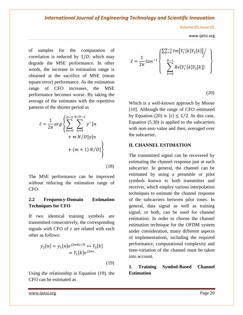
of samples for the computation of

correlation is reduced by 1/𝐷, which may

degrade the MSE performance. In other

words, the increase in estimation range is

obtained at the sacrifice of MSE (mean

square error) performance. As the estimation

range of CFO increases, the MSE

performance becomes worse. By taking the

average of the estimates with the repetitive

patterns of the shorter period as

휀̂ =1

2𝜋𝑎𝑟𝑔 {∑ ∑ 𝑦∗

𝑁 𝐷⁄ −1

𝑛=0

[𝑛

𝐷−2

𝑚=0

+𝑚𝑁 𝐷⁄ ]𝑦[𝑛

+ (𝑚 + 1)𝑁 𝐷⁄ ]}

(18)

The MSE performance can be improved

without reducing the estimation range of

CFO.

2.2 Frequency-Domain Estimation

Techniques for CFO

If two identical training symbols are

transmitted consecutively, the corresponding

signals with CFO of 휀 are related with each

other as follows:

𝑦2[𝑛] = 𝑦1[𝑛]𝑒𝑗2𝜋𝑁 𝑁⁄ ↔ 𝑌2[𝑘]

= 𝑌1[𝑘]𝑒𝑗2𝜋

(19)

Using the relationship in Equation (19), the

CFO can be estimated as

휀̂ =1

2𝜋𝑡𝑎𝑛−1

{

∑ 𝐼𝑚[𝑌1

∗[𝑘]𝑌2[𝑘]]𝑁−1𝑘=0 ⁄

∑𝑅𝑒[𝑌1∗[𝑘]𝑌2[𝑘]]

𝑁−1

𝑘=0 }

(20)

Which is a well-known approach by Moose

[10]. Although the range of CFO estimated

by Equation (20) is |휀| ≤ 1 2⁄ . In this case,

Equation (5.30) is applied to the subcarriers

with non-zero value and then, averaged over

the subcarrier.

II. CHANNEL ESTIMATION

The transmitted signal can be recovered by

estimating the channel response just at each

subcarrier. In general, the channel can be

estimated by using a preamble or pilot

symbols known to both transmitter and

receiver, which employ various interpolation

techniques to estimate the channel response

of the subcarriers between pilot tones. In

general, data signal as well as training

signal, or both, can be used for channel

estimation. In order to choose the channel

estimation technique for the OFDM system

under consideration, many different aspects

of implementations, including the required

performance, computational complexity and

time-variation of the channel must be taken

into account.

1. Training Symbol-Based Channel

Estimation


Volume:01,Issue:01

www.ijetsi.org


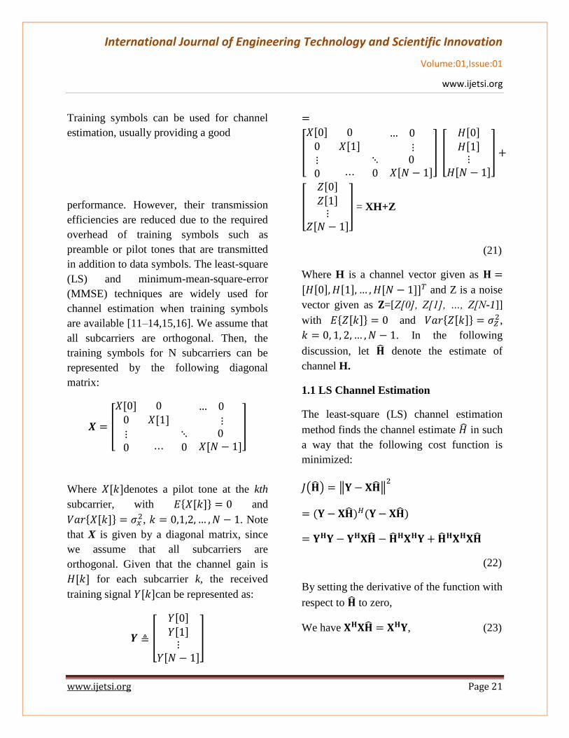
Training symbols can be used for channel

estimation, usually providing a good

performance. However, their transmission

efficiencies are reduced due to the required

overhead of training symbols such as

preamble or pilot tones that are transmitted

in addition to data symbols. The least-square

(LS) and minimum-mean-square-error

(MMSE) techniques are widely used for

channel estimation when training symbols

are available [11–14,15,16]. We assume that

all subcarriers are orthogonal. Then, the

training symbols for N subcarriers can be

represented by the following diagonal

matrix:

𝑿 = [

𝑋[0] 0 … 00 𝑋[1] ⋮⋮0 ⋯

⋱0

0𝑋[𝑁 − 1]

]

Where 𝑋[𝑘]denotes a pilot tone at the kth

subcarrier, with 𝐸{𝑋[𝑘]} = 0 and

𝑉𝑎𝑟{𝑋[𝑘]} = 𝜎𝑥2, 𝑘 = 0,1,2, … ,𝑁 − 1. Note

that X is given by a diagonal matrix, since

we assume that all subcarriers are

orthogonal. Given that the channel gain is

𝐻[𝑘] for each subcarrier k, the received

training signal 𝑌[𝑘]can be represented as:

𝒀 ≜ [

𝑌[0]

𝑌[1]⋮

𝑌[𝑁 − 1]

]

=

[

𝑋[0] 0 … 00 𝑋[1] ⋮⋮0 ⋯

⋱0

0𝑋[𝑁 − 1]

] [

𝐻[0]

𝐻[1]⋮

𝐻[𝑁 − 1]

] +

[

𝑍[0]

𝑍[1]⋮

𝑍[𝑁 − 1]

] = XH+Z

(21)

Where H is a channel vector given as 𝐇 =

[𝐻[0], 𝐻[1], … , 𝐻[𝑁 − 1]]𝑇 and Z is a noise

vector given as 𝐙=[Z[0], Z[1], …, Z[N-1]]

with 𝐸{𝑍[𝑘]} = 0 and 𝑉𝑎𝑟{𝑍[𝑘]} = 𝜎𝑍2,

𝑘 = 0, 1, 2, … ,𝑁 − 1. In the following

discussion, let �̂� denote the estimate of

channel H.

1.1 LS Channel Estimation

The least-square (LS) channel estimation

method finds the channel estimate �̂� in such

a way that the following cost function is

minimized:

𝐽(�̂�) = ‖𝐘 − 𝐗�̂�‖2

= (𝐘 − 𝐗�̂�)𝐻(𝐘 − 𝐗�̂�)

= 𝐘𝐇𝐘 − 𝐘𝐇𝐗�̂� − �̂�𝐇𝐗𝐇𝐘 + �̂�𝐇𝐗𝐇𝐗�̂�

(22)

By setting the derivative of the function with

respect to �̂� to zero,

We have 𝐗𝐇𝐗�̂� = 𝐗𝐇𝐘, (23)


Volume:01,Issue:01

www.ijetsi.org


which gives the solution to the LS channel

estimation as:

�̂�𝐋𝐒 = (𝐗𝐇𝐗)−𝟏𝐗𝐇𝐘 = 𝐗−𝟏𝐘

(24)

Let us denote each component of the LS

channel estimate �̂�𝐋𝐒 by �̂�𝐿𝑆[𝑘], k=0, 1, 2,

…, N-1.

Since X is assumed to be diagonal due to the

ICI-free condition, the LS channel estimate

�̂�𝐋𝐒 can be written for each subcarrier as:

�̂�𝐿𝑆[𝑘] =𝑌[𝑘]

𝑋[𝑘], 𝑘 = 0, 1, 2, … ,𝑁 − 1

(25)

The mean-square error (MSE) of this LS

channel estimate is given as

𝑀𝑆𝐸𝐿𝑆 = 𝐸{(𝐻 − �̂�𝐿𝑆)𝐻(𝐻 − 𝐻𝐿𝑆)}

= 𝐸{(𝐻 − 𝑋−1𝑌)𝐻(𝐻 − 𝑋−1𝑌)}

= 𝐸{(𝑋−1𝑍)𝐻(𝑋−1𝑍)}

= 𝐸{𝑍𝐻(𝑋𝑋𝐻)−1𝑍}

=𝜎𝑧2

𝜎𝑥2

(26)

Note that the MSE in Equation (26) is

inversely proportional to the SNR 𝜎𝑥2

𝜎𝑧2, which

implies that it may be subject to noise

enhancement, especially when the channel is

in a deep null. Due to its simplicity,

however, the LS method has been widely

used for channel estimation.

1.2 MMSE Channel Estimation

Consider the LS solution in Equation (24),

�̂�𝐋𝐒 = 𝐗−𝟏𝐘 ≜ �̃�. Using the weight matrix

W, define

�̂� ≜ 𝐖�̃�, which corresponds to the MMSE

estimate. MSE of the channel estimate �̂� is

given as

𝐽(�̂�) = 𝐸{‖𝑒‖2} = 𝐸 {‖𝐻 − �̂�‖2}

(27)

Then, the MMSE channel estimation method

finds a better (linear) estimate in terms of W

in such a way that the MSE in Equation (27)

is minimized. The orthogonality principle

states that the estimation error vector 𝐞 =

𝐇 − �̂� is orthogonal to �̃�, such that

𝐸{𝐞�̃�𝐇} = 𝐸{(𝐇 − �̂�)�̃�𝐇}

= 𝐸{(𝐇 −𝐖�̃�)�̃�𝐇}

= 𝐸{𝐇�̃�𝐇} −𝐖𝐸{�̃��̃�𝐇}

= 𝐑𝐇�̃� −𝐖𝐑�̃��̃� = 0

(28)

Where RAB is the cross-correlation matrix of

N x N matrices A and B (i.e., RAB =

𝐸[𝐀𝐁𝐻]), and �̃� is the LS channel estimate

given as

�̃� = 𝐗−𝟏𝐘 = 𝐇 + 𝐗−𝟏𝐙

(29)

Solving Equation (28) for W yields


Volume:01,Issue:01

www.ijetsi.org


𝐖 = 𝐑𝐇�̃�𝐑�̃��̃�−𝟏

(30)

Where 𝐑�̃��̃� is the autocorrelation matrix of

�̃� given as

𝐑�̃��̃� = 𝐸 {�̃��̃�𝐑}

= 𝐸{𝐑−𝐑𝐑(𝐑−𝐑𝐑)𝐸}

= 𝐸{(𝐑+𝐑−𝐑𝐑)(𝐑+𝐑−𝐑𝐑)𝐸}

= 𝐸{𝐑𝐑𝐸 +𝐑−𝐑𝐑𝐑𝐸

+𝐑𝐑𝐸(𝐑−𝐑)𝐸

+𝐑−𝐑𝐑𝐑𝐸(𝐑−𝐑)𝐸)}

(31)

= 𝐸{𝐑𝐑𝐸} +𝐸{𝐑−𝐑𝐑𝐑𝐸(𝐑−𝐑)𝐸}

= 𝐸{𝐑𝐑𝐸} +𝐸𝐸

2

𝐸𝐸2𝐑

And 𝐑𝐑�̃� is the cross-correlation matrix

between the true channel vector and

temporary channel estimate vector in the

frequency domain. Using Equation (31), the

MMSE channel estimate follows as

�̂� = 𝐑�̃� = 𝐑𝐑�̃�𝐑�̃��̃�−𝐑�̃�

= 𝐑𝐑�̃� (𝐑𝐑𝐑 +𝐸𝐸

2

𝐸𝐸2𝐑)

−𝐑

�̃�

(32)

The elements of 𝐑𝐑�̃� and 𝐑𝐑𝐑 in Equation

(6.14) are

𝐸{𝐸𝐸,𝐸�̃�𝐸′,𝐸′∗

} = 𝐸 {𝐸𝐸,𝐸𝐸𝐸′,𝐸′∗ }

= 𝐸𝐸[𝐸−𝐸′]𝐸 𝐸[𝐸−𝐸′]

(33)

Where k and l denote the subcarrier

(frequency) index and OFDM symbol (time)

index, respectively. In an exponentially-

decreasing multipath PDP (Power Delay

Profile), the frequency-domain correlation

𝐸𝐸[𝐸] is given as

𝐸𝐸[𝐸]

=1

1+𝐸2𝐸𝐸𝐸𝐸𝐸𝐸∆𝐸 (34)

where ∆𝐸 = 1 𝐸𝐸𝐸𝐸⁄ is the subcarrier

spacing for the FFT interval length of 𝐸𝐸𝐸𝑏.

Meanwhile, for a fading channel with the

maximum Doppler frequency 𝐸𝐸𝐸𝐸 and

Jake’s spectrum, the time-domain

correlation 𝐸 𝐸[𝐸] is given as

𝐸 𝐸[𝐸] = 𝐸0(2𝐸 𝐸𝐸𝐸𝐸 𝐸𝐸𝐸𝐸⁄ )

(35)

Where 𝐸𝐸𝐸𝐸 = 𝐸𝐸𝐸𝐸 +𝐸𝐸 for guard

interval time of 𝐸𝐸 and 𝐸0(𝐸) is the first

kind of 0th-order Bessel function. Note that

𝐸 𝐸[0] = 𝐸0(𝐸) =1.

To estimate the channel for data symbols,

the pilot subcarriers must be interpolated.

Popular interpolation methods include linear

interpolation, second-order polynomial

interpolation, and cubic spline interpolation

[13,14,17,18].

2. DFT-Based Channel Estimation


Volume:01,Issue:01

www.ijetsi.org


The DFT-based channel estimation

technique has been derived to improve the

performance of LS or MMSE channel

estimation by eliminating the effect of noise

outside the maximum channel delay. Let

�̂�[𝐸]denote the estimate of channel gain at

the kth subcarrier, obtained by either LS or

MMSE channel estimation method. Taking

the IDFT of the channel estimate

{�̂�[𝐸]}𝐸=0𝐸−1,

IDFT{�̂�[𝐸]} = 𝐸[𝐸]} +𝐸[𝐸] ≜ �̂�[𝐸],

𝐸 = 0, 1, 2, … ,𝐸− 1

(36)

Where z[n] denotes the noise component in

the time domain. Ignoring the coefficients

�̂�[𝐸] that contain the noise only, define the

coefficients for the maximum channel delay

L as

�̂�𝐸𝐸𝐸[𝐸]

= {𝐸[𝐸] +𝐸[𝐸], 𝐸 = 0, 1, 2, … ,𝐸− 1

0, 𝐸𝐸𝐸𝐸𝐸𝐸𝐸𝐸𝐸

(37)

And transform the remaining L elements

back to the frequency domain as follows

[19–22]:

�̂�𝐸𝐸𝐸[𝐸] = DFT{�̂�𝐸𝐸𝐸[𝐸]}

(38)

III. SIMULATION RESULTS

1. STO Estimation

In the simulation we test the performance of

CP-based STO estimation with the Number

of samples corresponding to STO is

nSTO=[-3 -3 3 3] and CFO= [0.00 0.50].

Fig.1: Performance of CP-based STO

estimation for nSTO=-3 and CFO=0.00:

maximum correlation-based vs minimum

difference-based estimation.


estimation for nSTO=-3 and CFO=0.50:




Volume:01,Issue:01

www.ijetsi.org



estimation for nSTO=3 and CFO=0.00:




estimation for nSTO=3 and CFO=0.50:



Fig.5: Performance of STO estimation from

difference between CP (cyclic prefix) and

rear part of OFDM symbol

Fig.5: Performance of STO estimation from

difference between CP (cyclic prefix) and

rear part of OFDM symbol

the results obtained by STO estimation using

CP, in which CFO is located at the point of

minimizing the difference between the

sample blocks of CP and that of data part or

maximizing their correlation.

2. Channel Estimation

In this part, we will test the performance of

LS-linear, LS-spline and MMSE with DFT


Volume:01,Issue:01

www.ijetsi.org


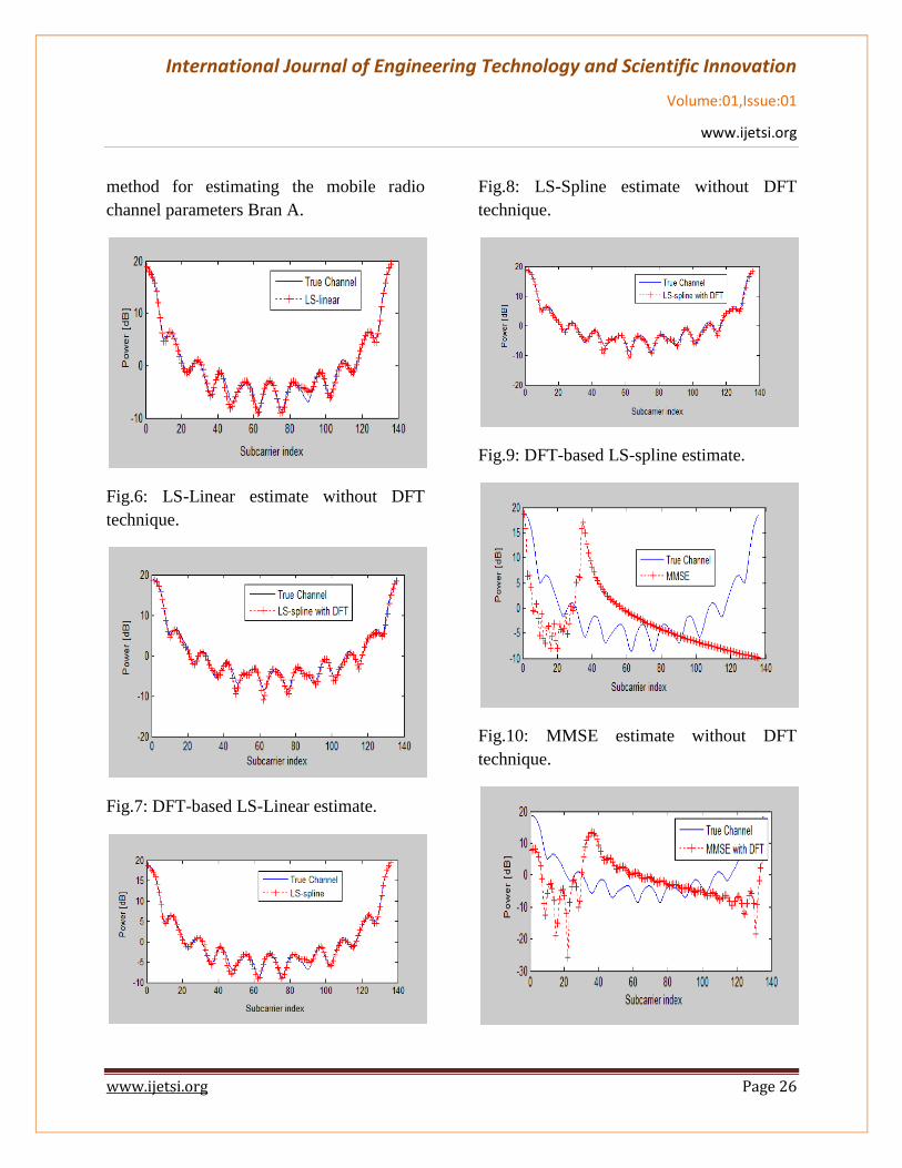
method for estimating the mobile radio

channel parameters Bran A.

Fig.6: LS-Linear estimate without DFT

technique.

Fig.7: DFT-based LS-Linear estimate.

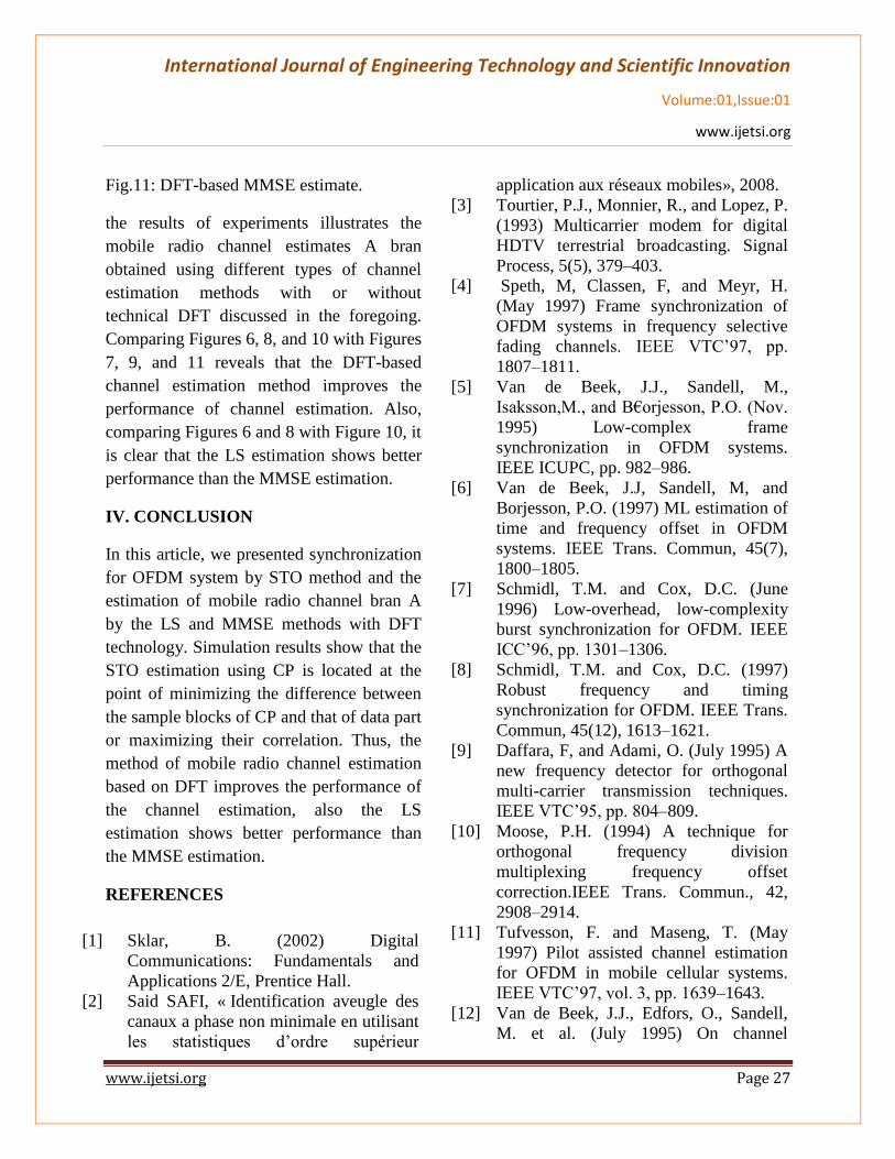
Fig.8: LS-Spline estimate without DFT

technique.

Fig.9: DFT-based LS-spline estimate.

Fig.10: MMSE estimate without DFT

technique.


Volume:01,Issue:01

www.ijetsi.org


Fig.11: DFT-based MMSE estimate.

the results of experiments illustrates the

mobile radio channel estimates A bran

obtained using different types of channel

estimation methods with or without

technical DFT discussed in the foregoing.

Comparing Figures 6, 8, and 10 with Figures

7, 9, and 11 reveals that the DFT-based

channel estimation method improves the

performance of channel estimation. Also,

comparing Figures 6 and 8 with Figure 10, it

is clear that the LS estimation shows better

performance than the MMSE estimation.

IV. CONCLUSION

In this article, we presented synchronization

for OFDM system by STO method and the

estimation of mobile radio channel bran A

by the LS and MMSE methods with DFT

technology. Simulation results show that the

STO estimation using CP is located at the

point of minimizing the difference between

the sample blocks of CP and that of data part

or maximizing their correlation. Thus, the

method of mobile radio channel estimation

based on DFT improves the performance of

the channel estimation, also the LS

estimation shows better performance than

the MMSE estimation.

REFERENCES

[1] Sklar, B. (2002) Digital

Communications: Fundamentals and

Applications 2/E, Prentice Hall.

[2]

Said SAFI, « Identification aveugle des

canaux a phase non minimale en utilisant

les statistiques d’ordre supérieur

[3]

application aux réseaux mobiles», 2008.

Tourtier, P.J., Monnier, R., and Lopez, P.

(1993) Multicarrier modem for digital

HDTV terrestrial broadcasting. Signal

Process, 5(5), 379–403.

[4]

Speth, M, Classen, F, and Meyr, H.

(May 1997) Frame synchronization of

OFDM systems in frequency selective

fading channels. IEEE VTC’97, pp.

1807–1811.

[5] Van de Beek, J.J., Sandell, M.,

Isaksson,M., and B€orjesson, P.O. (Nov.

1995) Low-complex frame

synchronization in OFDM systems.

IEEE ICUPC, pp. 982–986.

[6] Van de Beek, J.J, Sandell, M, and

Borjesson, P.O. (1997) ML estimation of

time and frequency offset in OFDM

systems. IEEE Trans. Commun, 45(7),

1800–1805.

[7] Schmidl, T.M. and Cox, D.C. (June

1996) Low-overhead, low-complexity

burst synchronization for OFDM. IEEE

ICC’96, pp. 1301–1306.

[8] Schmidl, T.M. and Cox, D.C. (1997)

Robust frequency and timing

synchronization for OFDM. IEEE Trans.

Commun, 45(12), 1613–1621.

[9] Daffara, F, and Adami, O. (July 1995) A

new frequency detector for orthogonal

multi-carrier transmission techniques.

IEEE VTC’95, pp. 804–809.

[10] Moose, P.H. (1994) A technique for

orthogonal frequency division

multiplexing frequency offset

correction.IEEE Trans. Commun., 42,

2908–2914.

[11] Tufvesson, F. and Maseng, T. (May

1997) Pilot assisted channel estimation

for OFDM in mobile cellular systems.

IEEE VTC’97, vol. 3, pp. 1639–1643.

[12]

Van de Beek, J.J., Edfors, O., Sandell,

M. et al. (July 1995) On channel


Volume:01,Issue:01

www.ijetsi.org


[13]

[14]

[15]

[16]

[17]

[18]

[19]

[20]

[21]

estimation in OFDM systems. IEEE

VTC’95, vol. 2, pp. 815–819.

Coleri, S., Ergen, M., Puri, A., and

Bahai, A. (2002) Channel estimation

techniques based on pilot arrangement in

OFDM systems. IEEE Trans. on

Broadcasting, 48(3), 223–229.

Heiskala, J. and Terry, J. (2002) OFDM

Wireless LANs: A Theoretical and

Practical Guide, SAMS.

van Nee, R. and Prasad, R. (2000)

OFDM for Wireless Multimedia

Communications, Artech House

Publishers.

Lau, H.K. and Cheung, S.W. (May 1994)

A pilot symbol-aided technique used for

digital signals in multipath

environments. IEEE ICC’94, vol. 2, pp.

1126–1130.

Van de Beek, J.J, Edfors, O, Sandell, M.

et al. (July 1995) On channel estimation

in OFDM systems. IEEE VTC’95, vol.

2, pp. 815–819.

Yang, W.Y., Cao, W., Chung, T.S., and

Morris, J. (2005) Applied Numerical

Methods Using MATLAB, John Wiley

& Sons, Inc., New York.

Minn, H. and Bhargava, V.K. (1999) An

investigation into time-domain approach

for OFDM channel estimation. IEEE

Trans. on Broadcasting, 45(4), 400–409.

Fernandez-Getino Garcia, M.J., Paez

[22]

Borrallo, J.M., and Zazo, S. (May 2001)

DFT-based channel estimation in 2D-

pilot-symbol-aided OFDM wireless

systems. IEEE VTC’01, vol. 2, pp. 810–

814.

van de Beek, J.J., Edfors, O., Sandell, M.

et al. (2000) Analysis of DFT-based

channel estimators for OFDM. Personal

Wireless Commun., 12(1), 55–70.

Zhao, Y. and Huang, A. (May 1998) A

novel channel estimation method for

OFDM mobile communication systems

based on pilot signals and transform-

domain processing. IEEE VTC’98, vol.

46, pp.931–939.

Documents

CHANNEL ESTIMATION AND SYNCHRONIZATION FOR OFDM … · CHANNEL ESTIMATION AND SYNCHRONIZATION FOR OFDM SYSTEM ... (wireless) channel The ... choose the channel estimation technique