Embed Size (px)
Citation preview

Simplified Channel Estimation
Techniques for OFDM Systems with
Realistic Indoor Fading Channels
by
Jake Hwang
A thesis
presented to the University of Waterloo
in fulfillment of the
thesis requirement for the degree of
Master of Applied Science
in
Electrical and Computer Engineering
Waterloo, Ontario, Canada, 2009
c©Jake Hwang, 2009

I hereby declare that I am the sole author of this thesis. This is a true copy of the thesis,
including any required final revisions, as accepted by my examiners.
I understand that my thesis may be made electronically available to the public.
Jake Hwang
ii
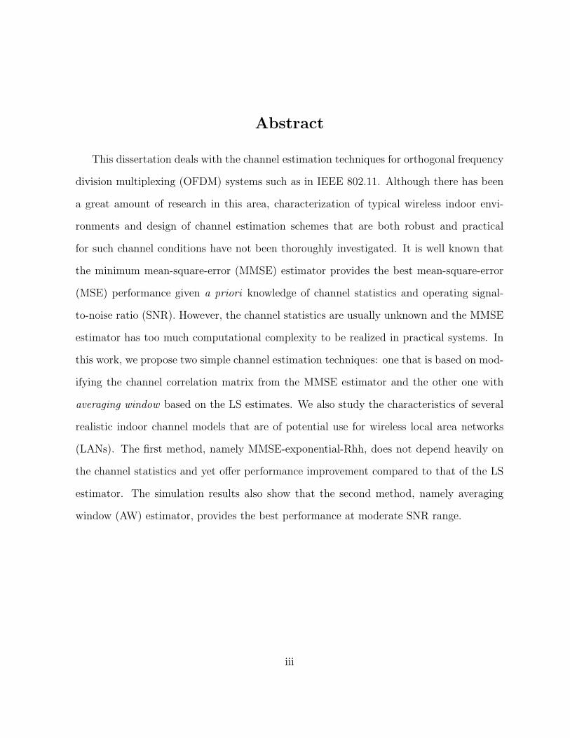
Abstract
This dissertation deals with the channel estimation techniques for orthogonal frequency
division multiplexing (OFDM) systems such as in IEEE 802.11. Although there has been
a great amount of research in this area, characterization of typical wireless indoor envi-
ronments and design of channel estimation schemes that are both robust and practical
for such channel conditions have not been thoroughly investigated. It is well known that
the minimum mean-square-error (MMSE) estimator provides the best mean-square-error
(MSE) performance given a priori knowledge of channel statistics and operating signal-
to-noise ratio (SNR). However, the channel statistics are usually unknown and the MMSE
estimator has too much computational complexity to be realized in practical systems. In
this work, we propose two simple channel estimation techniques: one that is based on mod-
ifying the channel correlation matrix from the MMSE estimator and the other one with
averaging window based on the LS estimates. We also study the characteristics of several
realistic indoor channel models that are of potential use for wireless local area networks
(LANs). The first method, namely MMSE-exponential-Rhh, does not depend heavily on
the channel statistics and yet offer performance improvement compared to that of the LS
estimator. The simulation results also show that the second method, namely averaging
window (AW) estimator, provides the best performance at moderate SNR range.
iii

Acknowledgments
I would like to thank my supervisor, Prof. Amir K. Khandani, for his valuable guidance
and support throughout the course of my graduate studies. His passion towards research
and care for his student have made this work possible. I would like to thank my readers,
Prof. Boumaiza and Prof. Safavi, for their valuable reviews, insights, and suggestions.
I would also like to thank my colleagues at CST lab for their insightful discussions and
supports.
I would like to thank my family for their unconditional love and belief in me. Lastly,
my special thank goes to the love of my life, Hyaewon Jeon. Without her love, I would
have not been where I am.
iv
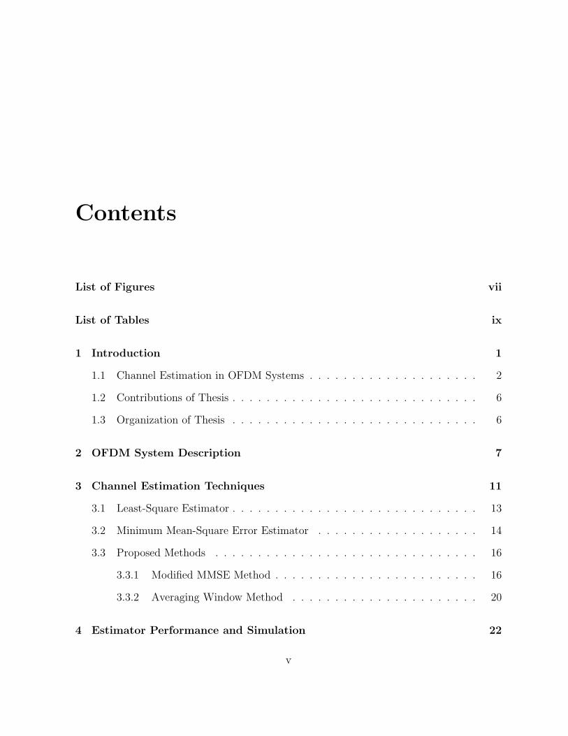
Contents
List of Figures vii
List of Tables ix
1 Introduction 1
1.1 Channel Estimation in OFDM Systems . . . . . . . . . . . . . . . . . . . . 2
1.2 Contributions of Thesis . . . . . . . . . . . . . . . . . . . . . . . . . . . . . 6
1.3 Organization of Thesis . . . . . . . . . . . . . . . . . . . . . . . . . . . . . 6
2 OFDM System Description 7
3 Channel Estimation Techniques 11
3.1 Least-Square Estimator . . . . . . . . . . . . . . . . . . . . . . . . . . . . . 13
3.2 Minimum Mean-Square Error Estimator . . . . . . . . . . . . . . . . . . . 14
3.3 Proposed Methods . . . . . . . . . . . . . . . . . . . . . . . . . . . . . . . 16
3.3.1 Modified MMSE Method . . . . . . . . . . . . . . . . . . . . . . . . 16
3.3.2 Averaging Window Method . . . . . . . . . . . . . . . . . . . . . . 20
4 Estimator Performance and Simulation 22
v
4.1 Channel Models and Scenarios . . . . . . . . . . . . . . . . . . . . . . . . . 22
4.1.1 Measurement Setup . . . . . . . . . . . . . . . . . . . . . . . . . . . 23
4.1.2 Measurement Environments . . . . . . . . . . . . . . . . . . . . . . 26
4.1.3 Measured Channel Frequency Responses . . . . . . . . . . . . . . . 28
4.2 Simulation Settings . . . . . . . . . . . . . . . . . . . . . . . . . . . . . . . 36
4.3 MSE Performance . . . . . . . . . . . . . . . . . . . . . . . . . . . . . . . . 38
4.3.1 Significance of ρ in MMSE-Exponential-Rhh Method . . . . . . . . 46
4.3.2 Significance of the Averaging Window Size in AW Method . . . . . 47
4.4 BER Performance . . . . . . . . . . . . . . . . . . . . . . . . . . . . . . . . 48
5 Conclusion and Future Work 51
A BER Performance for All Channel Models 53
References 54
vi
List of Figures
2.1 Baseband OFDM . . . . . . . . . . . . . . . . . . . . . . . . . . . . . . . . 8
2.2 The OFDM system, modeled as parallel Gaussian channels . . . . . . . . . 10
3.1 Two different types of pilot arrangement: (a) block-type pilot arrangement
and (b) comb-type pilot arrangement . . . . . . . . . . . . . . . . . . . . . 11
3.2 The channel correlation of the attenuation at m = 1 with the rest of atten-
uations in case where N = 64, τrms = 15ns, τmax = 80ns, and ρ = 0.98 . . . 20
4.1 The WARP board as the IEEE 802.11 interface . . . . . . . . . . . . . . . 24
4.2 The OFDM packet structure for WARP implementation . . . . . . . . . . 24
4.3 The equipment setup for channel measurement . . . . . . . . . . . . . . . . 25
4.4 Layout of the channel scenarios at South-East wing of DC building . . . . 27
4.5 Channel frequency response for channel model (a) A1, (b) A2, (c) B1, (d)
B2, (e) C1, (f) C2, (g) D1, (h) D2, (i) E1, and (j) E2 . . . . . . . . . . . . 33
4.6 Variance of channel frequency response over time . . . . . . . . . . . . . . 35
4.7 Normalized MSE for channel model A1 . . . . . . . . . . . . . . . . . . . . 39
4.8 Normalized MSE for channel model A2 . . . . . . . . . . . . . . . . . . . . 40
4.9 Normalized MSE for channel model B1 . . . . . . . . . . . . . . . . . . . . 40
vii
4.10 Normalized MSE for channel model B2 . . . . . . . . . . . . . . . . . . . . 41
4.11 Normalized MSE for channel model C1 . . . . . . . . . . . . . . . . . . . . 41
4.12 Normalized MSE for channel model C2 . . . . . . . . . . . . . . . . . . . . 42
4.13 Normalized MSE for channel model D1 . . . . . . . . . . . . . . . . . . . . 42
4.14 Normalized MSE for channel model D2 . . . . . . . . . . . . . . . . . . . . 43
4.15 Normalized MSE for channel model E1 . . . . . . . . . . . . . . . . . . . . 43
4.16 Normalized MSE for channel model E2 . . . . . . . . . . . . . . . . . . . . 44
4.17 Effects of averaging window size for channel model C1 . . . . . . . . . . . . 45
4.18 Correlation parameter ρ for each channel model . . . . . . . . . . . . . . . 46
4.19 Influence of ρ in MMSE-exponential-Rhh estimator for channel model A1 . 47
4.20 Relationship between the averaging window size and the frequency selectivity 48
4.21 BER performance for channel model A1 . . . . . . . . . . . . . . . . . . . 49
4.22 BER performance for channel model C2 . . . . . . . . . . . . . . . . . . . 50
A.1 BER performance for channel model A1 . . . . . . . . . . . . . . . . . . . 53
A.2 BER performance for channel model A2 . . . . . . . . . . . . . . . . . . . 54
A.3 BER performance for channel model B1 . . . . . . . . . . . . . . . . . . . 55
A.4 BER performance for channel model B2 . . . . . . . . . . . . . . . . . . . 55
A.5 BER performance for channel model C1 . . . . . . . . . . . . . . . . . . . 56
A.6 BER performance for channel model C2 . . . . . . . . . . . . . . . . . . . 56
A.7 BER performance for channel model D1 . . . . . . . . . . . . . . . . . . . 57
A.8 BER performance for channel model D2 . . . . . . . . . . . . . . . . . . . 57
A.9 BER performance for channel model E1 . . . . . . . . . . . . . . . . . . . 58
A.10 BER performance for channel model E2 . . . . . . . . . . . . . . . . . . . 58
viii
List of Tables
4.1 TGn Channel Model by the IEEE 802.11 . . . . . . . . . . . . . . . . . . . 23
4.2 Description of channel scenarios . . . . . . . . . . . . . . . . . . . . . . . . 26
4.3 OFDM system parameters . . . . . . . . . . . . . . . . . . . . . . . . . . . 36
4.4 Indoor channel models using tapped delay line . . . . . . . . . . . . . . . . 37
ix
Chapter 1
Introduction
Multimedia wireless services require high data-rate transmission over mobile radio channels.
Orthogonal Frequency Division Multiplexing (OFDM) is widely considered as a promising
choice for future wireless communications systems due to its high-data-rate transmission
capability with high bandwidth efficiency. In OFDM, the entire channel is divided into
many narrow subchannels, converting a frequency-selective channel into a collection of
frequency-flat channels. Moreover, intersymbol interference (ISI) is avoided by the use of
cyclic prefix (CP), which is achieved by extending an OFDM symbol with some portion
of its head or tail [16]. In fact, OFDM has been adopted in digital audio broadcasting
(DAB), digital video broadcasting (DVB), digital subscriber line (DSL), and wireless local
area network (WLAN) standards such as the IEEE 802.11a/b/g/n [1–4]. It has also been
adopted for wireless broadband access standards such as the IEEE 802.16e [5], and as the
core technique for the fourth-generation (4G) wireless mobile Communications [26].
To eliminate the need for channel estimation and tracking, differential phase-shift keying
(DPSK) can be used in OFDM systems. However, this results in a 3 dB loss in signal-
1
2 Introduction
to-noise ratio (SNR) compared with coherent demodulation such as phase-shift keying
(PSK) [37]. The performance of OFDM systems can be improved by allowing for coherent
demodulation when an accurate channel estimation technique is used.
1.1 Channel Estimation in OFDM Systems
Channel estimation techniques for OFDM systems can be grouped into two categories:
blind and non-blind. The blind channel estimation method exploits the statistical be-
haviour of the received signals, while the non-blind channel estimation method utilizes
some or all portions of the transmitted signals, i.e., pilot tones or training sequences,
which are available to the receiver to be used for the channel estimation.
The main advantage of the blind channel estimation is the possible elimination of train-
ing sequences, which decrease the system bandwidth efficiency [18, 45]. Additionally, due to
the time-varying nature of the channel in some wireless applications, the training sequence
needs to be transmitted periodically, causing further loss of channel throughput. Due to
these reasons, reducing the number of training symbols becomes a major concern, and
the blind channel estimation algorithms have received considerable attention [18]. There
are several types of blind channel estimation techniques found in literature. For example,
the subspace-based algorithms using redundant linear precoding are considered in [40, 54]
and nonredundant linear precoding in [6, 36]. In these methods, a linear block precoder
is applied at the transmitter and the channel information is extracted by exploiting the
covariance matrix of the received signals. Other subspace-based blind channel estimators
make use of the cyclostationarity inherent in OFDM signal due to CP [11, 15, 19, 33, 51].
Specifically, the authors in [19] proposed a method based on the cyclostationarity property
1.1 Channel Estimation in OFDM Systems 3
of the time-varying correlation of the received data samples caused by the CP insertion at
the transmitter. Cai et al. [11], on the other hand, developed a noise subspace method by
utilizing the time-invariant correlation of the received data vector. Other than the use of
CP, the subspace-based blind channel estimation using virtual carriers in OFDM symbols
is also proposed in [29]. Although these blind channel estimation techniques may be a
desirable approach as they do not require training or pilot signals to increase the system
bandwidth and the channel throughput, they require, however, a large amount of data in
order to make a reliable stochastic estimation. Therefore, they suffer from high computa-
tional complexity and severe performance degradation in fast fading channel [8, 50, 53].
On the other hand, the non-blind channel estimation can be performed by either in-
serting pilot tones into all of the subcarriers of OFDM symbols with a specific period or
inserting pilot tones into some of the subcarriers for each OFDM symbol [39]. In the first
case, an OFDM symbol with pilot tones in all the subcarriers is often called a training
sequence and this type of pilot arrangement is referred to as block-type pilot arrangement.
Block-type channel estimation is usually developed under the assumption of slow fading
channel, where the channel is assumed to be constant over one or more OFDM symbol
periods. The channel estimation for this block-type pilot arrangement can be based on
Least Square (LS) or Minimum Mean-Square Error (MMSE) [22, 34, 52]. It is well known
that the MMSE estimator has good performance but suffers from a high computational
complexity. On the other hand, the LS estimator has low complexity, but its performance
is not as good as that of the MMSE estimator. In [22], the MMSE estimate has been
shown to give up to 4 dB gain in SNR over the LS estimate for the same mean square
error (MSE) of the channel estimation. To reduce the complexity of the MMSE estimator,
4 Introduction
Edfors et al. [34] applied the theory of optimal rank-reduction to linear MMSE estimator
by using the singular value decomposition (SVD) [41] and the frequency correlation of the
channel.
In the latter case of the non-blind channel estimation, the pilot tones are multiplexed
with the data within an OFDM symbol and it is referred to as comb-type pilot arrangement.
The comb-type channel estimation is performed to satisfy the need for the channel equal-
ization or tracking in fast fading scenario, where the channel changes even in one OFDM
period. The main idea in comb-type channel estimation is to first estimate the channel
conditions at the pilot subcarriers and then estimate the channel at the data subcarriers by
means of interpolation. The estimation of the channel at the pilot subcarriers can be based
on LS, MMSE or Least Mean-Square (LMS). Once channel coefficients are estimated at
the pilot subcarriers, they are tracked by using adaptive Wiener filters such as Normalized
Least Mean-Square (NLMS) and Recursive Least Square (RLS) [14]. In these methods,
the channel impulse response (CIR) taps are updated based on the cost functions defined
for NLMS and RLS. Although NLMS is less complex and less accurate compared to RLS,
care must be taken in RLS algorithm for oversampled systems, as the performance can be
faulty due to implicit matrix inversion needed during update operation [44]. In [20, 39], a
variety of interpolation schemes are investigated and compared, including linear interpo-
lation, second-order interpolation, low-pass interpolation, spline cubic interpolation, and
time domain interpolation. The authors showed that the performance among these inter-
polation techniques range from the best to the worst, as follows: low-pass, spline cubic,
time domain, second-order and linear interpolation. Regardless of the use of interpolation
scheme, the performance of the channel estimation using comb-type pilot arrangement is
1.1 Channel Estimation in OFDM Systems 5
directly influenced by the number and/or locations of pilot subcarriers used for the initial
estimation [35]. In other words, the number of pilot subcarriers needs to be high enough
such that the frequency spacing between the pilot subcarriers is smaller than the channel
coherence bandwidth in order to obtain a reliable estimation. Therefore, the comb-type
channel estimation may not be suitable for some applications, such as the wireless LANs
[1–4] where the number of pilot tones is too small compared to the number of data tones
and their locations are fixed.
Another type of non-blind channel estimation technique is called a Decision Directed
Channel Estimation (DDCE). The main idea behind DDCE is to use the channel estimation
of a previous OFDM symbol for the data detection of the current estimation, and thereafter
using the newly detected data for the estimation of the current channel [27, 32]. Once
the data at the subcarriers is detected, any methods described above can be used to
estimate the current channel. The major benefit of the DDCE scheme is that in contrast
to purely pilot assisted channel estimation methods, both the pilot symbols as well as all
the information symbols are utilized for channel estimation [9]. On the other hand, the
DDCE inherently introduces two basic problems: the use of outdated channel estimates,
and the assumption of correct data detection. The use of outdated channel estimates
does not pose a serious issue when the channel is varying very slowly. However, when the
channel starts varying faster, then the outdated channel estimates for the previous OFDM
symbol are no longer valid for the use of the data detection in the current OFDM symbol.
Hence, the error in the channel estimation and data detection build up to make the system
performance unacceptable [12]. In addition, this error propagation can be also amplified
by any discrepancies in the system, which limits its use in practical systems.
6 Introduction
1.2 Contributions of Thesis
This thesis focuses on the non-blind channel estimation techniques that are based on the
block-type pilot arrangement. Once we establish reliable and practical channel estimation
schemes for this type of pilot arrangement, we expect that our proposed schemes can
be simply applied to the systems with comb-type pilot arrangement (or DDCE) and use
the interpolation methods discussed previously. A second objective of this thesis is to
investigate the characteristics of the typical indoor environments in which actual wireless
network such as WLAN is deployed. Having understood the behaviour of radio propagation
in such environments, we then present the performance analysis of our proposed techniques.
1.3 Organization of Thesis
The remainder of this thesis is organized as follows. In Chapter 2, the OFDM system model
under investigation is described. In Chapter 3, we present the LS and MMSE estimator,
along with our proposed methods. We also remark on some interesting aspects of the
estimators. In Chapter 4, we investigate the realistic indoor channel models and analyze the
mean-square-error (MSE) and bit-error-rate (BER) performance of the proposed methods.
Design considerations and trade offs are also discussed in this chapter. Lastly, conclusions
and future research are presented in Chapter 5.
Chapter 2
OFDM System Description
The basic idea underlying OFDM systems is the division of the available frequency spec-
trum into several subcarriers, converting a frequency-selective channel into a parallel col-
lection of frequency flat subchannels [42]. To obtain a high spectral efficiency, the signal
spectra corresponding to the different subcarriers overlap in frequency, and yet they have
the minimum frequency separation to maintain orthogonality of their corresponding time
domain waveforms [17]. The use of a CP both preserves the orthogonality of the tones and
eliminates ISI between consecutive OFDM symbols.
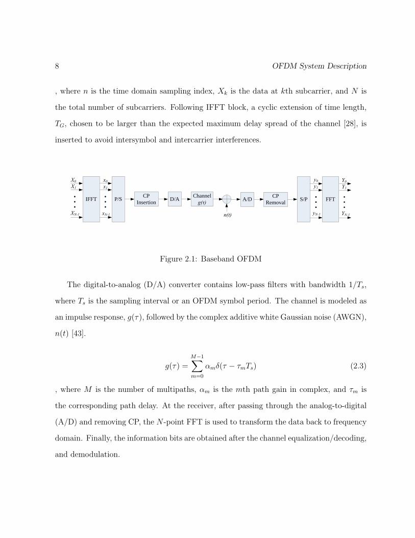
A block diagram of a baseband OFDM system is shown in Figure 2.1. After the
information bits are grouped, coded and modulated, they are fed into N -point inverse fast
Fourier transform (IFFT) to obtain the time domain OFDM symbols, i.e.,
xn = IFFTN {Xk} (2.1)
=N−1∑k=0
Xkej2πnk/N , 0 ≤ n, k ≤ N − 1 (2.2)
7
8 OFDM System Description
, where n is the time domain sampling index, Xk is the data at kth subcarrier, and N is
the total number of subcarriers. Following IFFT block, a cyclic extension of time length,
TG, chosen to be larger than the expected maximum delay spread of the channel [28], is
inserted to avoid intersymbol and intercarrier interferences.
IFFT
X0X1
XN-1
P/S CP Insertion D/A Channel
g(τ)
n(t)
A/D CP Removal S/P FFT
x0x1
xN-1
y0y1
yN-1
Y0Y1
YN-1
Figure 2.1: Baseband OFDM
The digital-to-analog (D/A) converter contains low-pass filters with bandwidth 1/Ts,
where Ts is the sampling interval or an OFDM symbol period. The channel is modeled as
an impulse response, g(τ), followed by the complex additive white Gaussian noise (AWGN),
n(t) [43].
g(τ) =M−1∑m=0
αmδ(τ − τmTs) (2.3)
, where M is the number of multipaths, αm is the mth path gain in complex, and τm is
the corresponding path delay. At the receiver, after passing through the analog-to-digital
(A/D) and removing CP, the N -point FFT is used to transform the data back to frequency
domain. Finally, the information bits are obtained after the channel equalization/decoding,
and demodulation.
9
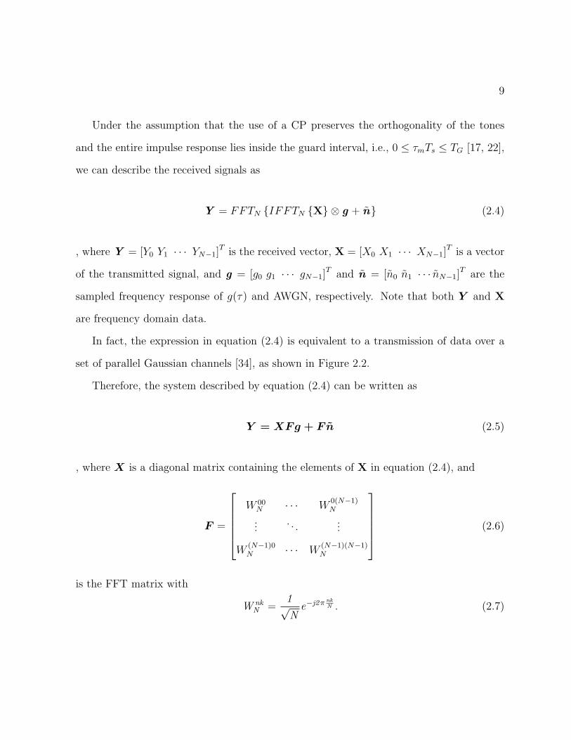
Under the assumption that the use of a CP preserves the orthogonality of the tones
and the entire impulse response lies inside the guard interval, i.e., 0 ≤ τmTs ≤ TG [17, 22],
we can describe the received signals as
Y = FFTN {IFFTN {X} ⊗ g + n} (2.4)
, where Y = [Y0 Y1 · · · YN−1]T is the received vector, X = [X0 X1 · · · XN−1]
T is a vector
of the transmitted signal, and g = [g0 g1 · · · gN−1]T and n = [n0 n1 · · · nN−1]
T are the
sampled frequency response of g(τ) and AWGN, respectively. Note that both Y and X
are frequency domain data.
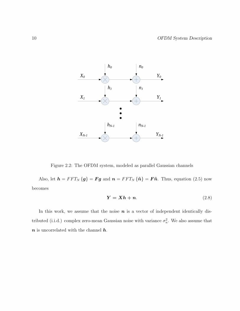
In fact, the expression in equation (2.4) is equivalent to a transmission of data over a
set of parallel Gaussian channels [34], as shown in Figure 2.2.
Therefore, the system described by equation (2.4) can be written as
Y = XFg + F n (2.5)
, where X is a diagonal matrix containing the elements of X in equation (2.4), and
F =
W 00N · · · W
0(N−1)N
.... . .
...
W(N−1)0N · · · W
(N−1)(N−1)N
(2.6)
is the FFT matrix with
W nkN =
1√N
e−j2π nkN . (2.7)
10 OFDM System Description
X0
h0 n0
Y0
X1
h1 n1
Y1
XN-1
hN-1 nN-1
YN-1
Figure 2.2: The OFDM system, modeled as parallel Gaussian channels
Also, let h = FFTN {g} = Fg and n = FFTN {n} = F n. Thus, equation (2.5) now
becomes
Y = Xh + n. (2.8)
In this work, we assume that the noise n is a vector of independent identically dis-
tributed (i.i.d.) complex zero-mean Gaussian noise with variance σ2n. We also assume that
n is uncorrelated with the channel h.
Chapter 3
Channel Estimation Techniques
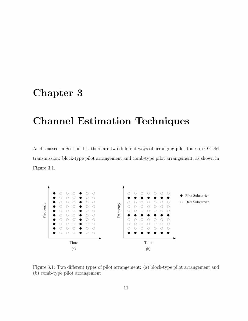
As discussed in Section 1.1, there are two different ways of arranging pilot tones in OFDM
transmission: block-type pilot arrangement and comb-type pilot arrangement, as shown in
Figure 3.1.
Time
Freq
uenc
y
Time
Freq
uenc
y Data Subcarrier
Pilot Subcarrier
(a) (b)
Figure 3.1: Two different types of pilot arrangement: (a) block-type pilot arrangement and(b) comb-type pilot arrangement
11
12 Channel Estimation Techniques
For the channel estimation based on block-type pilot arrangement, the spacing between
consecutive training sequences needs to be determined carefully. When the channel varies
across OFDM symbols in time, the training sequence must be inserted at a ratio that is
determined by the coherence time or Doppler spread. In [38], a quantitative expression,
based on the Nyquist sampling theorem for the maximum spacing of training sequence in
time, Nt,max, is given by
Nt,max ≤1
2nfD,maxTs(3.1)
, where n is the oversampling factor, fD,max, is the maximum Doppler spread, and Ts is
the OFDM symbol duration. Therefore, if the training sequence is inserted at the start of
the packet or block similar to those in WLAN, the packet length should be smaller than
Nt,maxTs in time.
Similarly, the spacing of pilot tones within an OFDM symbol, in the case of comb-type
channel estimation, should also be small enough so that the variations of the channel in
frequency can be captured. That is,
Nf,max ≤1
nτmax∆f(3.2)
, where τmax is the maximum delay spread and ∆f is the subcarrier spacing in OFDM
symbol. Here, the pilot spacing should be smaller than Nf,max∆f in frequency or simply
Nf,max subcarrier spacings in order to be able to perform an interpolation.
Regardless of which pilot arrangement scheme is used for the non-blind channel esti-
mation, the basic channel estimation technique is the same for both schemes. That is,
the comb-type pilot channel estimation can be treated as a special case of the block-type
3.1 Least-Square Estimator 13
pilot channel estimation, where the channel estimation technique is performed only at the
pilot subcarriers, followed by the interpolation at the data subcarriers. In this work, we
only consider the frequency domain initial channel estimation techniques based on the
block-type pilot arrangement, assuming equation (3.1) is satisfied.
In this chapter, the LS estimation technique is presented as it is needed by many
estimation techniques as an initial estimation, followed by the MMSE estimator. Then,
the modified MMSE estimator is proposed in an attempt to reduce the computational
complexity and eliminate the need for a priori knowledge of the channel statistics. We
also propose another simple and effective channel estimator which is based on the LS
estimate.
3.1 Least-Square Estimator
From equation (2.8), the LS estimator minimizes the following cost function [47]
minh
(Y − Xh)H
(Y − Xh) (3.3)
, where [·]H is the Hermitian (conjugate) transpose operator. Then, the LS estimation of
h is given by
hLS =Y
X=
[YkXk
]T(3.4)
, where [·]T is the transpose operator and k = 0, 1, · · · , N − 1. This LS estimator is
equivalent to what is also referred to as the zero-forcing estimator [22, 30] since it can also
be obtained from the time domain LS estimator with no assumption on the number of CIR
14 Channel Estimation Techniques
taps or length. That is,
hLS = FQLSFHXHY (3.5)
, where
QLS =(F HXHXF
)−1. (3.6)
Note that this simple LS estimator does not exploit the correlation of channel across
subcarriers in frequency and across the OFDM symbols in time. Without using any knowl-
edge of the statistics of the channel, the LS estimator can be calculated with very low
complexity, but it has a high mean-square error since it does not take into account of the
effect of noise on the signal.
3.2 Minimum Mean-Square Error Estimator
The minimum mean-square error is widely used in the OFDM channel estimation since it
is optimum in terms of mean square error (MSE) in the presence of AWGN [7]. In fact, it
is observed in [35] that many channel estimation techniques are indeed a subset of MMSE
channel estimation technique. The MMSE estimator employs the second-order statistics
of the channel, channel correlation function, and the operating SNR.
Let us define Rgg, Rhh, and RY Y as the autocovariance matrix of g, h, and Y , re-
spectively. We also define RgY as the crosscovariance matrix between g and Y . Assuming
the channel vector, h, and the noise vector, n, are uncorrelated, we derive that
Rhh = E{HHH
}= E
{(Fg)(Fg)H
}= FRggF
H , (3.7)
3.2 Minimum Mean-Square Error Estimator 15
RgY = E{gY H
}= E
{g(XFg + n)H
}= RggF
HXH (3.8)
, and
RY Y = E{Y Y H
}= XFRggF
HXH + σ2nIN (3.9)
where σ2n is the noise variance, E
{|n|2
}, and IN is the N ×N Identity matrix. Assuming
the channel correlation matrix, Rhh, and the operating SNR, σ2n, are known at the receiver,
the MMSE estimator of g is given by [22, 34, 39, 49]
gMMSE = RgY R−1Y Y Y . (3.10)
Finally, combining the above equations, the frequency domain MMSE estimator can be
calculated by
hMMSE = F gMMSE
= F [(FHXH)−1R−1gg σ
2n + XF ]−1Y
= FRgg[(FHXHXF )−1σ2n + Rgg]F −1hLS
= Rhh[Rhh + σ2n(XXH)−1]−1hLS. (3.11)
The above MMSE estimator yields much better performance than LS estimator, espe-
cially under the low SNR scenarios. However, a major drawback of the MMSE estimator
is its high computational complexity, since the matrix inversion of size N × N is needed
each time data in X changes.
Another drawback of this estimator is that it requires one to know the correlation of the
channel and the operating SNR in order to minimize the MSE between the transmitted and
16 Channel Estimation Techniques
received signals. However, in wireless links, the channel statistics depend on the particular
environment, for example, indoor or outdoor, Line-Of-Sight (LOS) or Non-Line-Of-Sight
(NLOS), and changes with time [52]. Therefore, MMSE estimator may not be feasible in
a practical system.
3.3 Proposed Methods
As discussed in the previous section, the channel estimation based on MMSE is the best
estimator in terms of MSE performance at a cost of high computational complexity. In
this section, we propose two different channel estimation techniques with low complexity
and robustness against channel conditions.
3.3.1 Modified MMSE Method
In addition to a high computational complexity, the MMSE estimator requires a priori
knowledge of the second-order statistics of the channel condition, i.e., the channel corre-
lation function across the frequency tones. Such information is embedded in the channel
correlation matrix Rhh from equation (3.11), which plays a critical role in reducing noise
that is added on top of the LS estimation.
First, we examine the expression of Rhh, proposed by Edfors et al. [34]:
Rhh = E{hhH
}= [rm,n] (3.12)
and
rm,n =1− e−τmax((1/τrms)+2πj(m−n)/N)
τrms(1− e−(τmax/τrms))( 1τrms
+ j2πm−nN
)(3.13)
3.3 Proposed Methods 17
, where m,n = 0, 1, · · · , N − 1, τrms is a root-mean square (rms) delay spread, and τmax
is the maximum delay spread. Here, it is assumed that an exponentially decaying power-
delay profile θ(τm) = Ce−τm/τrms and delays τm from equation (2.3) are uniformly and
independently distributed over the length of the maximum delay spread.
In practice, however, the true channel information and the corresponding delay spread
values are not known. Hence, as pointed out in [52], it is not robust to design a MMSE
estimator that tightly matches the channel statistics. It is also computationally very heavy
that it is not feasible to update Rhh every time the channel changes. Therefore, we propose
a different approach of modeling the channel correlation matrix, which is described in the
following section.
Exponential Rhh Model
Here, we adopt a concept of first-order finite-state Markov chain [10, 13] to represent the
channel correlation matrix Rhh, such that it eliminates the need for a priori knowledge of
the channel (rms/maximum delay spread and assumptions imposed on multipath delays)
and reduces the computational complexity, while it closely follows the behaviour of the
true channel correlation matrix. In general, a first-order Markov chain is widely used to
represent a slowly time-varying channel and defined by its initial-state occupancy prob-
abilities and its transition probabilities [25]. As stated in [48], the first-order Markovian
assumption implies that, given the information on the state immediately preceding the
current one, any other previous state should be independent of the current state. In our
case, we assume that the channel correlation matrix depends only on the correlation of two
consecutive channel attenuations (having a memory of 1), with such correlation parameter
18 Channel Estimation Techniques
being analogous to state in Markovian model. The correlation parameter ρ is modeled as
a magnitude of the channel autocorrelation function where the distance between the tones
is 1. For example,
ρ =∣∣E {hp+qh∗p}∣∣ =
∣∣∣∣∣N−q−1∑p=0
hp+qh∗p
∣∣∣∣∣ , q = 1. (3.14)
Then, a new channel correlation matrix Rhh is constructed such that its elements are
the exponential series of ρ. That is,
<{rm,n} =[ρ|m−n|
]
=
1 ρ ρ2 · · · ρN−1
ρ 1 ρ · · · ρN−2
......
...
ρN−1 ρN−2 ρN−3 · · · 1
(3.15)
and
={rm,n} =
[1− ρ|m−n|
], m ≤ n[
−(1− ρ|m−n|
)], otherwise
=
0 1− ρ 1− ρ2 · · · 1− ρN−1
−(1− ρ) 0 1− ρ · · · 1− ρN−2
......
...
−(1− ρN−1) −(1− ρN−2) −(1− ρN−3) · · · 0
(3.16)
, where m,n = 0, 1, · · · , N − 1. Combining equation (3.15) and equation (3.16), we have
3.3 Proposed Methods 19
Rhh as a form of symmetric or Hermitian Toeplitz matrix, same as Rhh. In this modi-
fication, we aim to remodel Rhh using properties of first-order Markov chain, such that
the new channel correlation matrix Rhh has similar properties as the true channel corre-
lation matrix Rhh, which is a correlation between the channel attenuations hm and hn,
not the data subcarriers Xm and Xn. The analytical comparison between Rhh and Rhh is
discussed in the following section.
Analysis of Channel Correlation Matrices
To illustrate the characteristics of the channel correlation matrices, Rhh and Rhh, let us
assume a system with N = 64 tones and a channel with τrms = 15ns and τmax = 80ns.
Since they are both Hermitian Toeplitz matrices, we will consider the elements on the first
row, which represent the correlation of the channel attenuation at the first tone m = 1
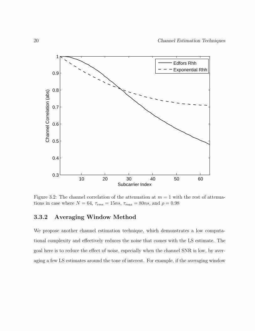
against the channel attenuations at the rest of the tones. As can be seen from Figure 3.2,
the correlation decreases as the distance of the tones m− n increases for Rhh (labeled as
Edfors Rhh).
For Rhh (labeled as Exponential Rhh), it behaves similarly to that of Rhh as the
correlation of channel attenuations decreases while the distance of the tones increases.
However, its correlation curve levels out for the second half of the tones. This can be
interpreted as the channel correlation being more or less the same for the tones with a
distance larger than N/2.
20 Channel Estimation Techniques
10 20 30 40 50 600.3
0.4
0.5
0.6
0.7
0.8
0.9
1
Subcarrier Index
Cha
nnel
Cor
rela
tion
(abs
)
Edfors RhhExponential Rhh
Figure 3.2: The channel correlation of the attenuation at m = 1 with the rest of attenua-tions in case where N = 64, τrms = 15ns, τmax = 80ns, and ρ = 0.98
3.3.2 Averaging Window Method
We propose another channel estimation technique, which demonstrates a low computa-
tional complexity and effectively reduces the noise that comes with the LS estimate. The
goal here is to reduce the effect of noise, especially when the channel SNR is low, by aver-
aging a few LS estimates around the tone of interest. For example, if the averaging window
3.3 Proposed Methods 21
size is M , the final estimate at the kth subcarrier can be expressed as
hAW ;k =1
M
∑i
hLS;i , k −⌊M
2
⌋≤ i ≤ k +
⌊M
2
⌋(3.17)
, where hLS;i is the LS estimate at the ith subcarrier. This method can be viewed as
an averaging window sliding across the tones that are circularly arranged. The size of
averaging window, M , should be carefully selected such that the Averaging Window (AW)
method minimizes the MSE for a given operating SNR, i.e., M should be large in the low
SNR range and small in the high SNR range. It should also depend on how much the
channel fluctuates across the tones (frequency selectivity). That is, the more frequency-
selective channel is, the smaller the averaging window should be. The relationship between
the averaging window size and frequency selectivity (along with SNR) is studied in the next
chapter.
Chapter 4
Estimator Performance and
Simulation
4.1 Channel Models and Scenarios
There has been much effort in indoor channel modeling by many different groups, such as
ETSI BRAN [23], ITU-R [31], and the IEEE 802.11 Working Group [46]. For example,
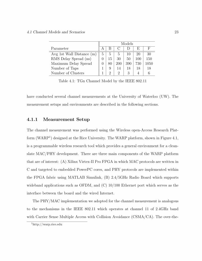
the popular TGn channel models developed by the IEEE 802.11 for indoor WLAN are
described in Table 4.1.
Although the channel models proposed by these institutes try to generalize the channel
statistics for different environments, they lack details about the measurement settings,
such as the shape or dimensions of the environment, physical orientation of obstacles, and
the whereabouts of Tx/Rx. In addition, none of these models investigates the channel
behaviour in other typical indoor environments, e.g., small/large office, corridor, or a large
open space like foyer. To understand the channel behaviour in such environments, we
22
4.1 Channel Models and Scenarios 23
ModelsParameter A B C D E F
Avg 1st Wall Distance (m) 5 5 5 10 20 30RMS Delay Spread (ns) 0 15 30 50 100 150Maximum Delay Spread 0 80 200 390 730 1050Number of Taps 1 9 14 18 18 18Number of Clusters 1 2 2 3 4 6
Table 4.1: TGn Channel Model by the IEEE 802.11
have conducted several channel measurements at the University of Waterloo (UW). The
measurement setups and environments are described in the following sections.
4.1.1 Measurement Setup
The channel measurement was performed using the Wireless open-Access Research Plat-
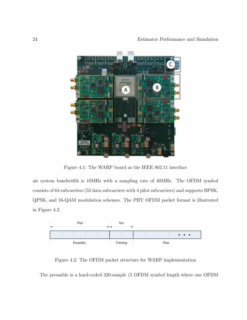
form (WARP1) designed at the Rice University. The WARP platform, shown in Figure 4.1,
is a programmable wireless research tool which provides a general environment for a clean-
slate MAC/PHY development. There are three main components of the WARP platform
that are of interest: (A) Xilinx Virtex-II Pro FPGA in which MAC protocols are written in
C and targeted to embedded PowerPC cores, and PHY protocols are implemented within
the FPGA fabric using MATLAB Simulink, (B) 2.4/5GHz Radio Board which supports
wideband applications such as OFDM, and (C) 10/100 Ethernet port which serves as the
interface between the board and the wired Internet.
The PHY/MAC implementation we adopted for the channel measurement is analogous
to the mechanisms in the IEEE 802.11 which operates at channel 11 of 2.4GHz band
with Carrier Sense Multiple Access with Collision Avoidance (CSMA/CA). The over-the-
1http://warp.rice.edu
24 Estimator Performance and Simulation
Figure 4.1: The WARP board as the IEEE 802.11 interface
air system bandwidth is 10MHz with a sampling rate of 40MHz. The OFDM symbol
consists of 64 subcarriers (52 data subcarriers with 4 pilot subcarriers) and supports BPSK,
QPSK, and 16-QAM modulation schemes. The PHY OFDM packet format is illustrated
in Figure 4.2.
20μs 8μs
Preamble Training Data
Figure 4.2: The OFDM packet structure for WARP implementation
The preamble is a hard-coded 320-sample (5 OFDM symbol length where one OFDM
4.1 Channel Models and Scenarios 25
symbol duration is 8 µs) sequence used by the receiver for AGC, carrier frequency offset
estimation and symbol timing estimation. This field is analogous to that of Short Training
Field (STF) in the IEEE 802.11a standard. The training field consists of a fixed sequence
repeated one after another (2 OFDM symbol length) and it is mainly used for channel
estimation, similar to Long Training Field (LTF) in the IEEE 802.11a. The channel es-
timation is performed such that the receiver independently estimates the channel using
the LS method (refer to Section 3.1) for each training period and averages them out to
produce a smoother channel estimate. This estimated channel is used for equalization and
decoding in the data part until the next packet arrives.
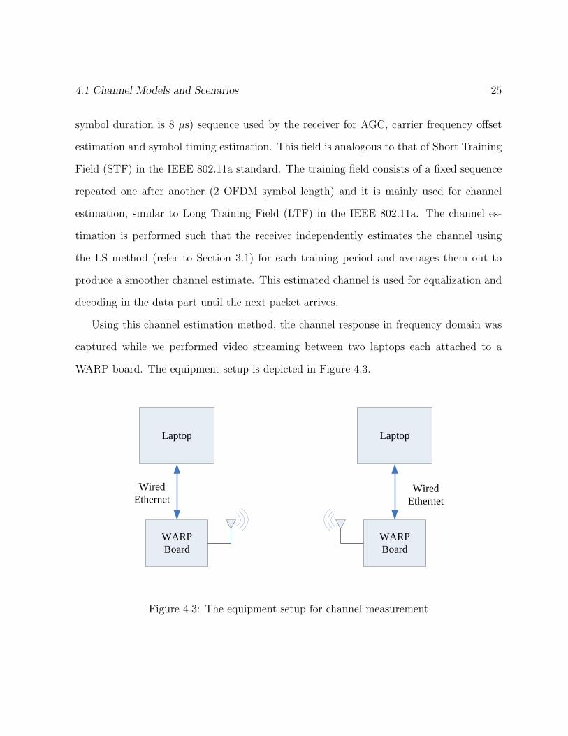
Using this channel estimation method, the channel response in frequency domain was
captured while we performed video streaming between two laptops each attached to a
WARP board. The equipment setup is depicted in Figure 4.3.
Laptop Laptop
WARPBoard
WARPBoard
WiredEthernet
WiredEthernet
Figure 4.3: The equipment setup for channel measurement
26 Estimator Performance and Simulation
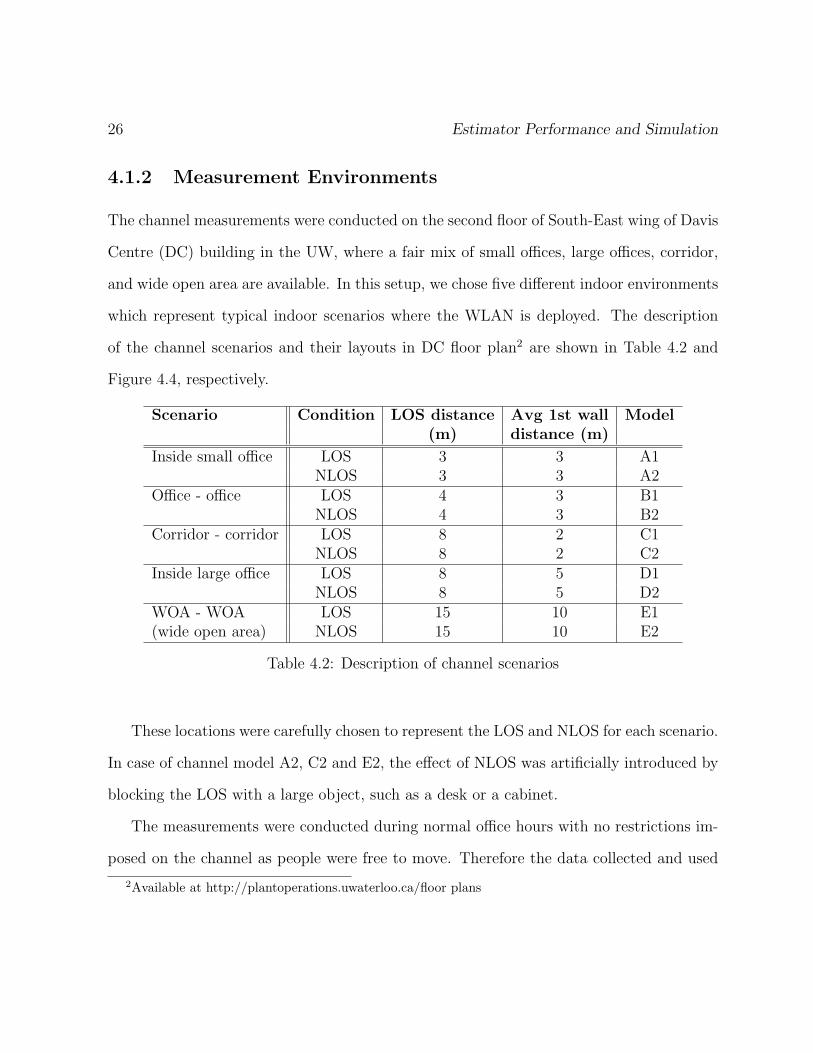
4.1.2 Measurement Environments
The channel measurements were conducted on the second floor of South-East wing of Davis
Centre (DC) building in the UW, where a fair mix of small offices, large offices, corridor,
and wide open area are available. In this setup, we chose five different indoor environments
which represent typical indoor scenarios where the WLAN is deployed. The description
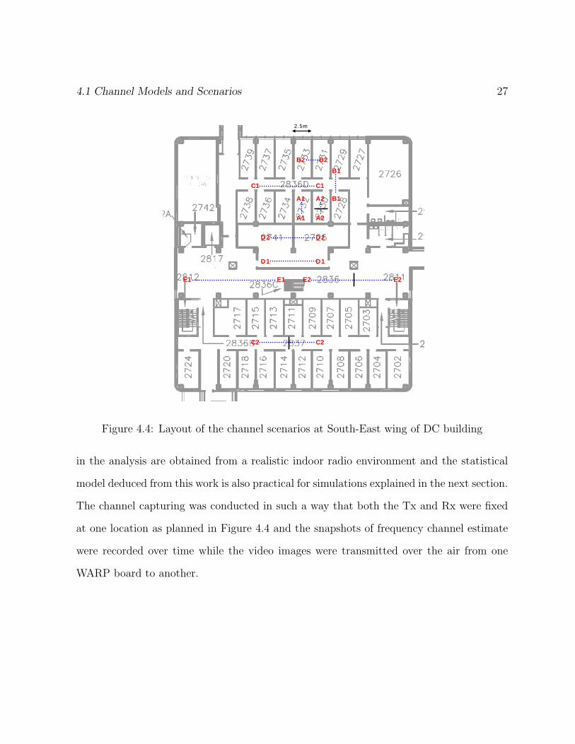
of the channel scenarios and their layouts in DC floor plan2 are shown in Table 4.2 and
Figure 4.4, respectively.
Scenario Condition LOS distance Avg 1st wall Model(m) distance (m)
Inside small office LOS 3 3 A1NLOS 3 3 A2
Office - office LOS 4 3 B1NLOS 4 3 B2
Corridor - corridor LOS 8 2 C1NLOS 8 2 C2
Inside large office LOS 8 5 D1NLOS 8 5 D2
WOA - WOA LOS 15 10 E1(wide open area) NLOS 15 10 E2
Table 4.2: Description of channel scenarios
These locations were carefully chosen to represent the LOS and NLOS for each scenario.
In case of channel model A2, C2 and E2, the effect of NLOS was artificially introduced by
blocking the LOS with a large object, such as a desk or a cabinet.
The measurements were conducted during normal office hours with no restrictions im-
posed on the channel as people were free to move. Therefore the data collected and used
2Available at http://plantoperations.uwaterloo.ca/floor plans
4.1 Channel Models and Scenarios 27
A2
A2
B1
B1
A1
A1
B2 B2
C1C1
D2D2
E2E2E1E1
D1D1
C2C2
2.5m
Figure 4.4: Layout of the channel scenarios at South-East wing of DC building
in the analysis are obtained from a realistic indoor radio environment and the statistical
model deduced from this work is also practical for simulations explained in the next section.
The channel capturing was conducted in such a way that both the Tx and Rx were fixed
at one location as planned in Figure 4.4 and the snapshots of frequency channel estimate
were recorded over time while the video images were transmitted over the air from one
WARP board to another.
28 Estimator Performance and Simulation
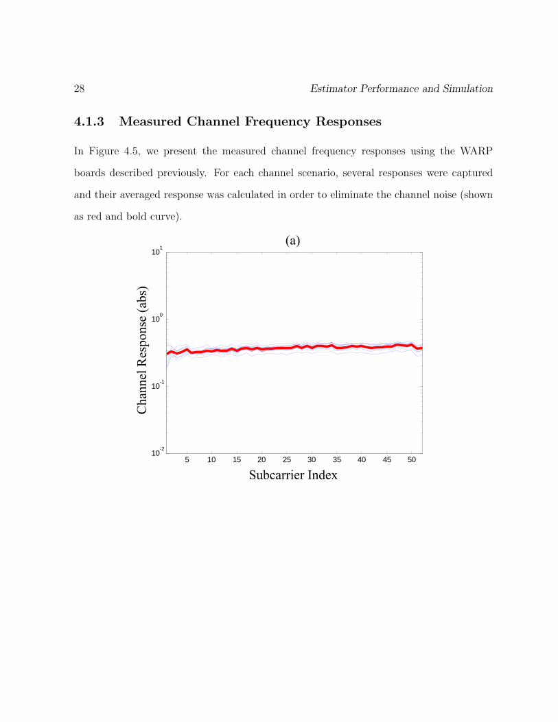
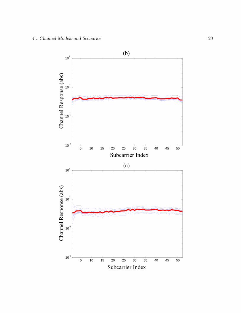
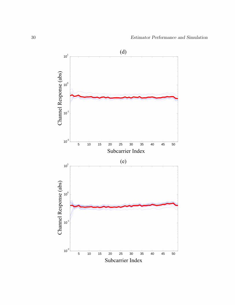
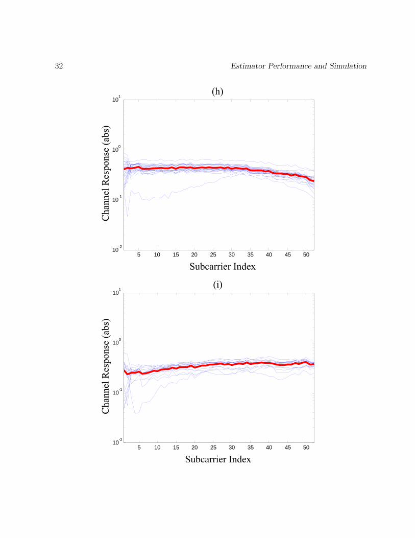
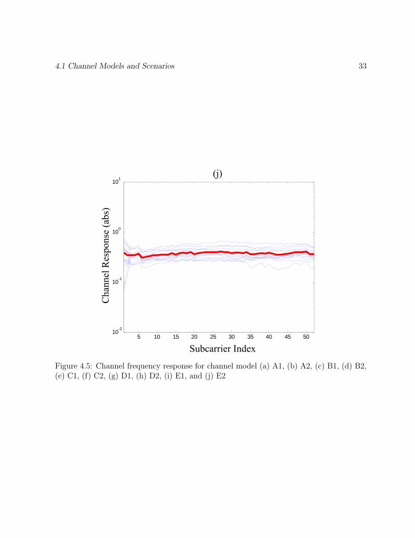
4.1.3 Measured Channel Frequency Responses
In Figure 4.5, we present the measured channel frequency responses using the WARP
boards described previously. For each channel scenario, several responses were captured
and their averaged response was calculated in order to eliminate the channel noise (shown
as red and bold curve).
5 10 15 20 25 30 35 40 45 5010-2
10-1
100
101
4.1 Channel Models and Scenarios 29
5 10 15 20 25 30 35 40 45 5010-2
10-1
100
101
5 10 15 20 25 30 35 40 45 5010-2
10-1
100
101
30 Estimator Performance and Simulation
5 10 15 20 25 30 35 40 45 5010-2
10-1
100
101
5 10 15 20 25 30 35 40 45 5010-2
10-1
100
101

4.1 Channel Models and Scenarios 31
5 10 15 20 25 30 35 40 45 5010-2
10-1
100
101
5 10 15 20 25 30 35 40 45 5010-2
10-1
100
101
32 Estimator Performance and Simulation
5 10 15 20 25 30 35 40 45 5010-2
10-1
100
101
5 10 15 20 25 30 35 40 45 5010-2
10-1
100
101
4.1 Channel Models and Scenarios 33
5 10 15 20 25 30 35 40 45 5010-2
10-1
100
101
Figure 4.5: Channel frequency response for channel model (a) A1, (b) A2, (c) B1, (d) B2,(e) C1, (f) C2, (g) D1, (h) D2, (i) E1, and (j) E2
34 Estimator Performance and Simulation
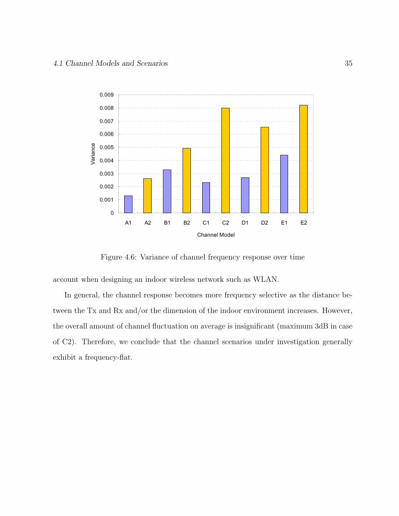
As shown in Figure 4.5, it is observed that the channel variations between consecutive
packets increase as the dimensions of indoor environment are increased. In other words,
the amount of variation from one channel response to another is increased over time.
For example, most of the channel responses in scenario A1 are concentrated around the
averaged response whereas many of responses deviating from the averaged response are
observed in scenario E1. This is an interesting observation as the channel exhibits a time
selectivity even though both Tx and Rx were set stationary for the entire time. Also, a
theoretical coherence time is much larger than the time difference between capturing each
consecutive responses. This can be explained by the fact that there are more traffic by
people and changes in environment in a large office (D) or wide open area (E) than an
area like a small office (A or B). To illustrate the finding more quantitatively, the variance
per subcarrier of all the channel responses is calculated and then they are averaged out
to represent the time variance for each channel scenario. In Figure 4.6, we see that the
time variance increases proportionally with the size of the indoor environment, and this
relationship is more evident in the NLOS cases. It is also observed that the variation is
larger in case of LOS than of NLOS for a given channel scenario. We can then conclude
that NLOS not only introduces frequency selectivity but also time selectivity in a wireless
radio channel.
Another interesting finding is observed in the channel model C2. The radio propagation
in a long and narrow indoor environment with very short distance to the surrounding
walls exhibits a similar behaviour as in wide-open-area environment, when there is no
dominant multipath component. This illustrates that the statistics of the channel are also
significantly affected by the specific indoor settings and these factors should be taken into
4.1 Channel Models and Scenarios 35
0
0.001
0.002
0.003
0.004
0.005
0.006
0.007
0.008
0.009
A1 A2 B1 B2 C1 C2 D1 D2 E1 E2
Channel Model
Varia
nce
Figure 4.6: Variance of channel frequency response over time
account when designing an indoor wireless network such as WLAN.
In general, the channel response becomes more frequency selective as the distance be-
tween the Tx and Rx and/or the dimension of the indoor environment increases. However,
the overall amount of channel fluctuation on average is insignificant (maximum 3dB in case
of C2). Therefore, we conclude that the channel scenarios under investigation generally
exhibit a frequency-flat.
36 Estimator Performance and Simulation
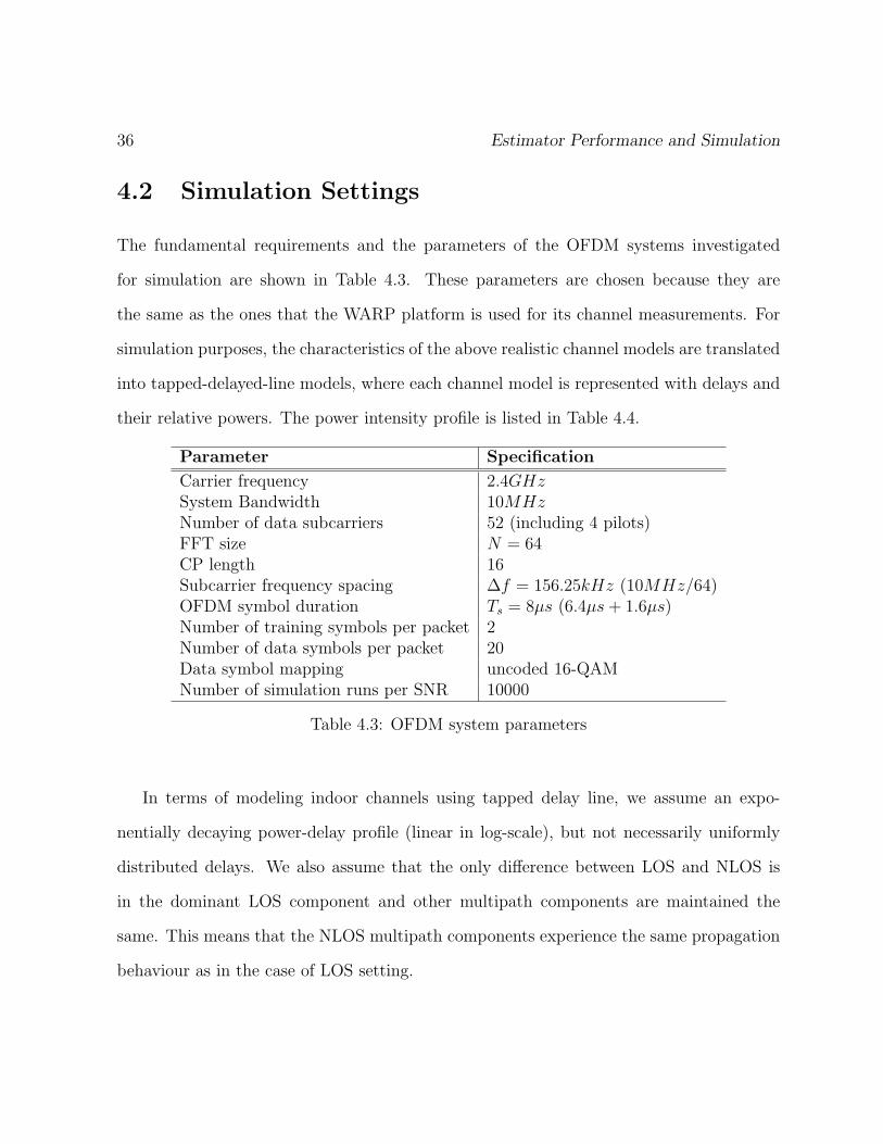
4.2 Simulation Settings
The fundamental requirements and the parameters of the OFDM systems investigated
for simulation are shown in Table 4.3. These parameters are chosen because they are
the same as the ones that the WARP platform is used for its channel measurements. For
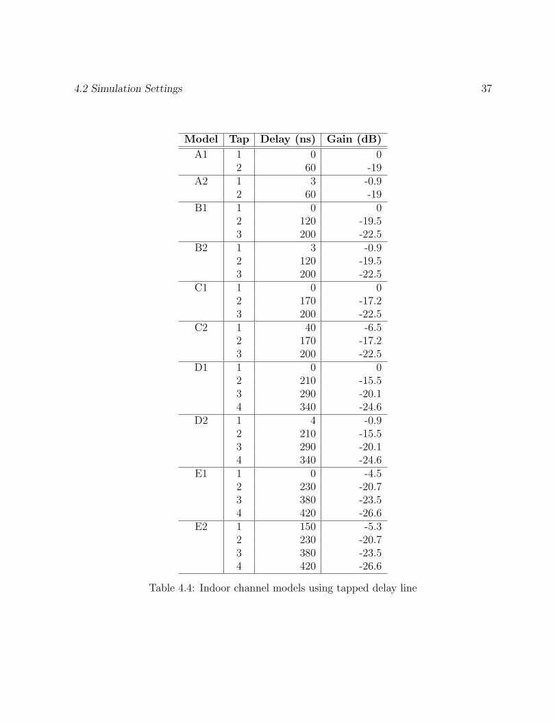
simulation purposes, the characteristics of the above realistic channel models are translated
into tapped-delayed-line models, where each channel model is represented with delays and
their relative powers. The power intensity profile is listed in Table 4.4.
Parameter Specification
Carrier frequency 2.4GHzSystem Bandwidth 10MHzNumber of data subcarriers 52 (including 4 pilots)FFT size N = 64CP length 16Subcarrier frequency spacing ∆f = 156.25kHz (10MHz/64)OFDM symbol duration Ts = 8µs (6.4µs+ 1.6µs)Number of training symbols per packet 2Number of data symbols per packet 20Data symbol mapping uncoded 16-QAMNumber of simulation runs per SNR 10000
Table 4.3: OFDM system parameters
In terms of modeling indoor channels using tapped delay line, we assume an expo-
nentially decaying power-delay profile (linear in log-scale), but not necessarily uniformly
distributed delays. We also assume that the only difference between LOS and NLOS is
in the dominant LOS component and other multipath components are maintained the
same. This means that the NLOS multipath components experience the same propagation
behaviour as in the case of LOS setting.
4.2 Simulation Settings 37
Model Tap Delay (ns) Gain (dB)
A1 1 0 02 60 -19
A2 1 3 -0.92 60 -19
B1 1 0 02 120 -19.53 200 -22.5
B2 1 3 -0.92 120 -19.53 200 -22.5
C1 1 0 02 170 -17.23 200 -22.5
C2 1 40 -6.52 170 -17.23 200 -22.5
D1 1 0 02 210 -15.53 290 -20.14 340 -24.6
D2 1 4 -0.92 210 -15.53 290 -20.14 340 -24.6
E1 1 0 -4.52 230 -20.73 380 -23.54 420 -26.6
E2 1 150 -5.32 230 -20.73 380 -23.54 420 -26.6
Table 4.4: Indoor channel models using tapped delay line
38 Estimator Performance and Simulation
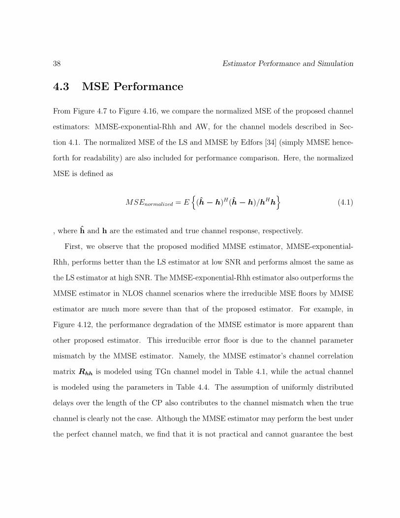
4.3 MSE Performance
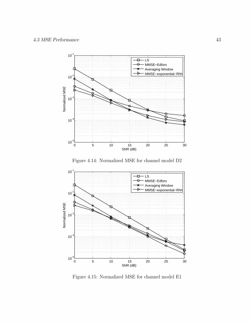
From Figure 4.7 to Figure 4.16, we compare the normalized MSE of the proposed channel
estimators: MMSE-exponential-Rhh and AW, for the channel models described in Sec-
tion 4.1. The normalized MSE of the LS and MMSE by Edfors [34] (simply MMSE hence-
forth for readability) are also included for performance comparison. Here, the normalized
MSE is defined as
MSEnormalized = E{
(h − h)H(h − h)/hHh}
(4.1)
, where h and h are the estimated and true channel response, respectively.
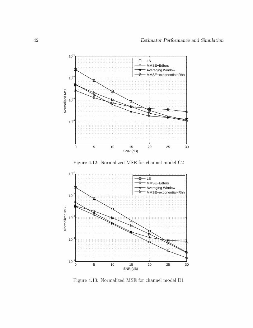
First, we observe that the proposed modified MMSE estimator, MMSE-exponential-
Rhh, performs better than the LS estimator at low SNR and performs almost the same as
the LS estimator at high SNR. The MMSE-exponential-Rhh estimator also outperforms the
MMSE estimator in NLOS channel scenarios where the irreducible MSE floors by MMSE
estimator are much more severe than that of the proposed estimator. For example, in
Figure 4.12, the performance degradation of the MMSE estimator is more apparent than
other proposed estimator. This irreducible error floor is due to the channel parameter
mismatch by the MMSE estimator. Namely, the MMSE estimator’s channel correlation
matrix Rhh is modeled using TGn channel model in Table 4.1, while the actual channel
is modeled using the parameters in Table 4.4. The assumption of uniformly distributed
delays over the length of the CP also contributes to the channel mismatch when the true
channel is clearly not the case. Although the MMSE estimator may perform the best under
the perfect channel match, we find that it is not practical and cannot guarantee the best
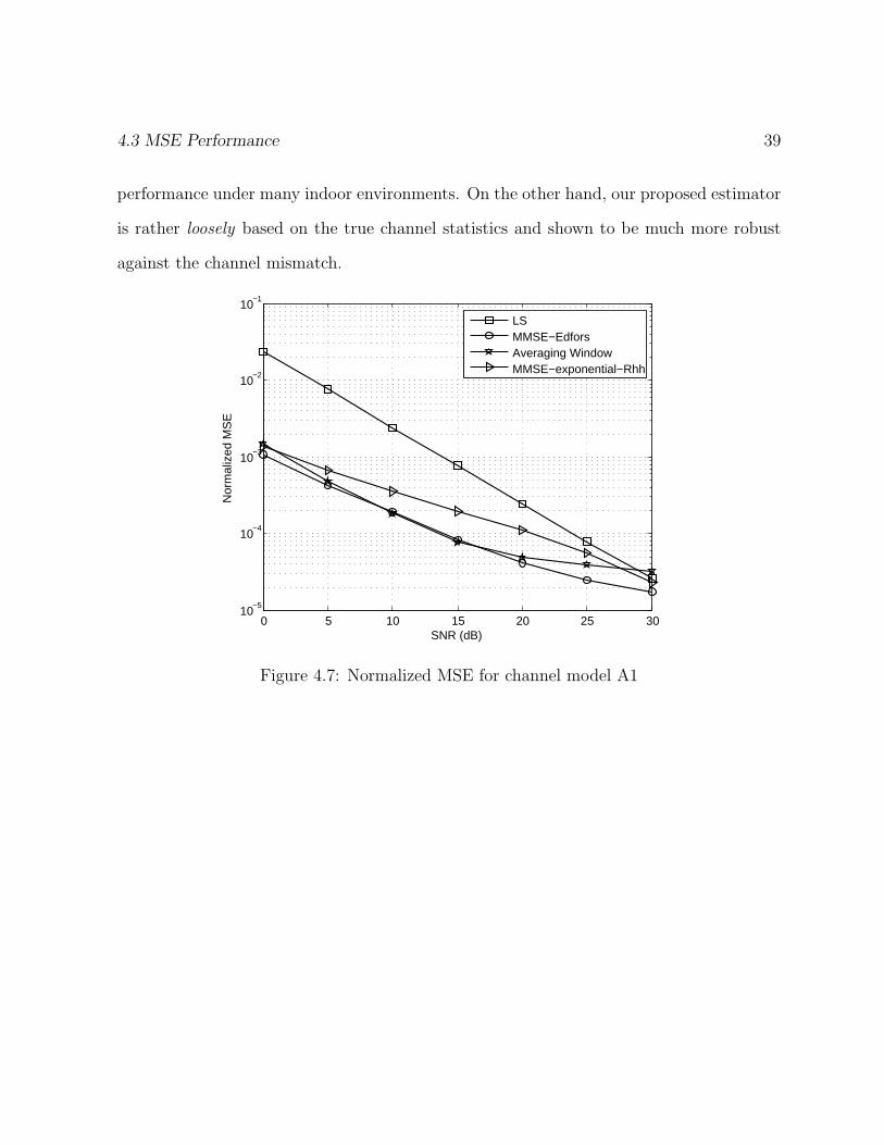
4.3 MSE Performance 39
performance under many indoor environments. On the other hand, our proposed estimator
is rather loosely based on the true channel statistics and shown to be much more robust
against the channel mismatch.
0 5 10 15 20 25 3010
−5
10−4
10−3
10−2
10−1
SNR (dB)
Nor
mal
ized
MS
E
LSMMSE−EdforsAveraging WindowMMSE−exponential−Rhh
Figure 4.7: Normalized MSE for channel model A1
40 Estimator Performance and Simulation
0 5 10 15 20 25 3010
−5
10−4
10−3
10−2
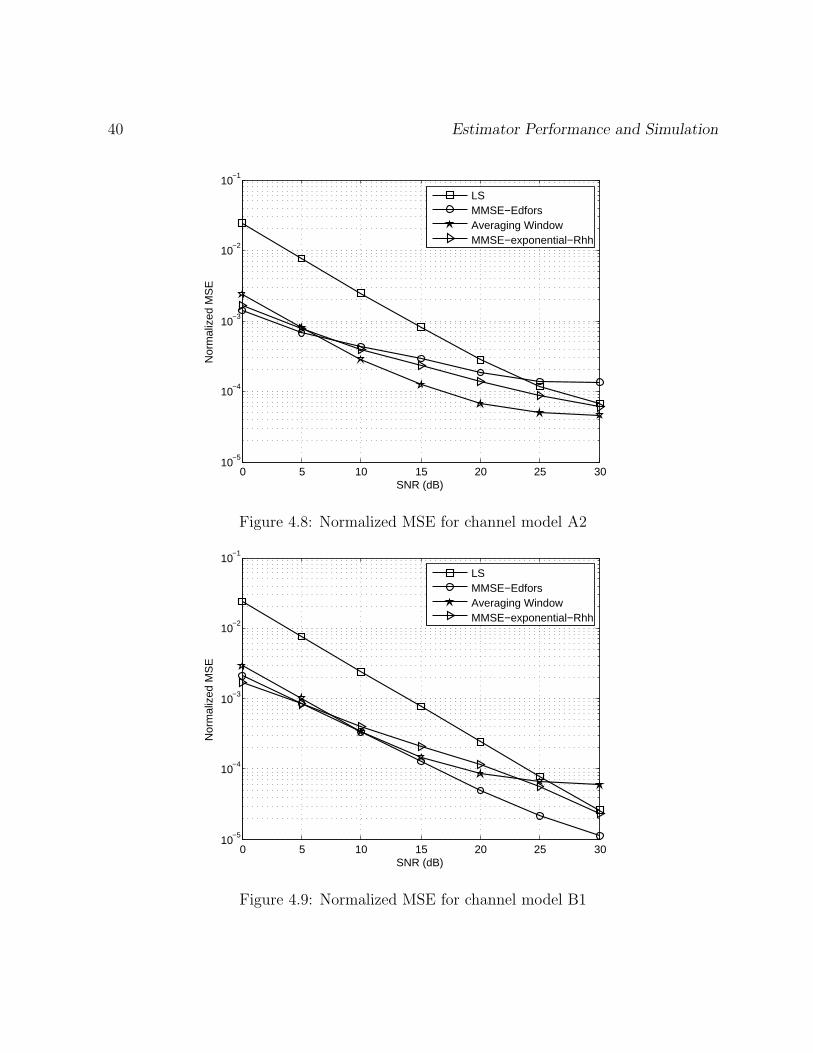
10−1
SNR (dB)
Nor
mal
ized
MS
E
LSMMSE−EdforsAveraging WindowMMSE−exponential−Rhh
Figure 4.8: Normalized MSE for channel model A2
0 5 10 15 20 25 3010
−5
10−4
10−3
10−2
10−1
SNR (dB)
Nor
mal
ized
MS
E
LSMMSE−EdforsAveraging WindowMMSE−exponential−Rhh
Figure 4.9: Normalized MSE for channel model B1

4.3 MSE Performance 41
0 5 10 15 20 25 3010
−5
10−4
10−3
10−2
10−1
SNR (dB)
Nor
mal
ized
MS
E
LSMMSE−EdforsAveraging WindowMMSE−exponential−Rhh
Figure 4.10: Normalized MSE for channel model B2
0 5 10 15 20 25 3010
−5
10−4
10−3
10−2
10−1
SNR (dB)
Nor
mal
ized
MS
E
LSMMSE−EdforsAveraging WindowMMSE−exponential−Rhh
Figure 4.11: Normalized MSE for channel model C1
42 Estimator Performance and Simulation
0 5 10 15 20 25 30
10−4
10−3
10−2
10−1
SNR (dB)
Nor
mal
ized
MS
E
LSMMSE−EdforsAveraging WindowMMSE−exponential−Rhh
Figure 4.12: Normalized MSE for channel model C2
0 5 10 15 20 25 3010
−5
10−4
10−3
10−2
10−1
SNR (dB)
Nor
mal
ized
MS
E
LSMMSE−EdforsAveraging WindowMMSE−exponential−Rhh
Figure 4.13: Normalized MSE for channel model D1
4.3 MSE Performance 43
0 5 10 15 20 25 3010
−5
10−4
10−3
10−2
10−1
SNR (dB)
Nor
mal
ized
MS
E
LSMMSE−EdforsAveraging WindowMMSE−exponential−Rhh
Figure 4.14: Normalized MSE for channel model D2
0 5 10 15 20 25 3010
−5
10−4
10−3
10−2
10−1
SNR (dB)
Nor
mal
ized
MS
E
LSMMSE−EdforsAveraging WindowMMSE−exponential−Rhh
Figure 4.15: Normalized MSE for channel model E1
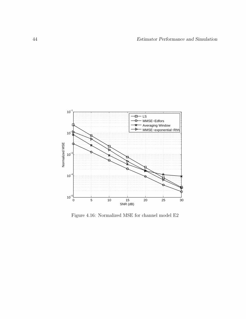
44 Estimator Performance and Simulation
0 5 10 15 20 25 3010
−5
10−4
10−3
10−2
10−1
SNR (dB)
Nor
mal
ized
MS
E
LSMMSE−EdforsAveraging WindowMMSE−exponential−Rhh
Figure 4.16: Normalized MSE for channel model E2
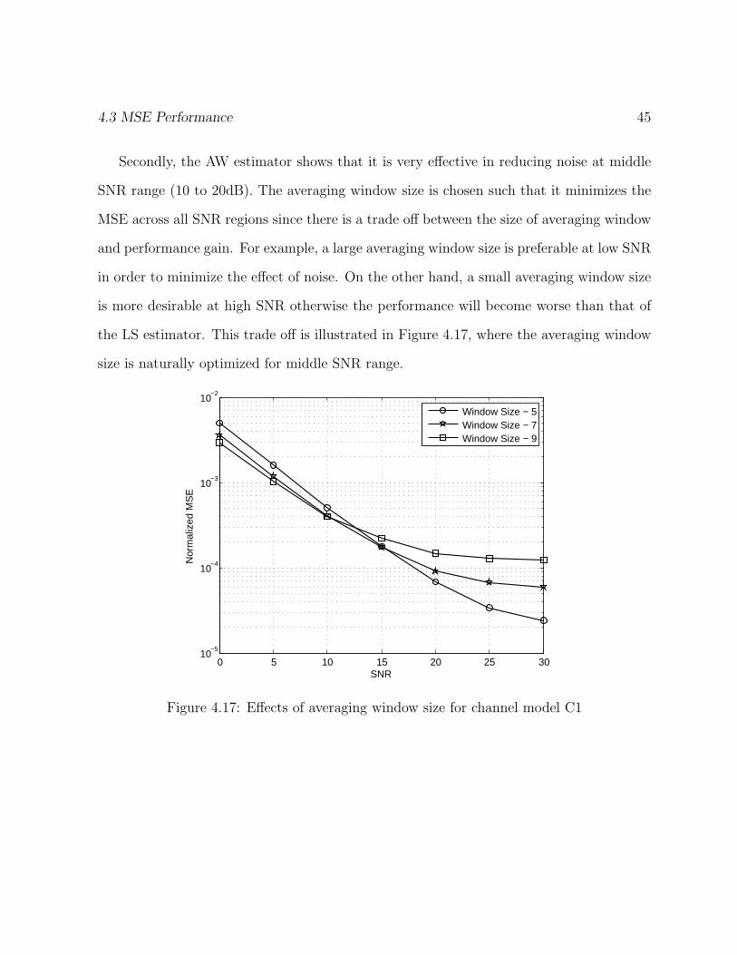
4.3 MSE Performance 45
Secondly, the AW estimator shows that it is very effective in reducing noise at middle
SNR range (10 to 20dB). The averaging window size is chosen such that it minimizes the
MSE across all SNR regions since there is a trade off between the size of averaging window
and performance gain. For example, a large averaging window size is preferable at low SNR
in order to minimize the effect of noise. On the other hand, a small averaging window size
is more desirable at high SNR otherwise the performance will become worse than that of
the LS estimator. This trade off is illustrated in Figure 4.17, where the averaging window
size is naturally optimized for middle SNR range.
0 5 10 15 20 25 3010
−5
10−4
10−3
10−2
SNR
Nor
mal
ized
MS
E
Window Size − 5Window Size − 7Window Size − 9
Figure 4.17: Effects of averaging window size for channel model C1
46 Estimator Performance and Simulation
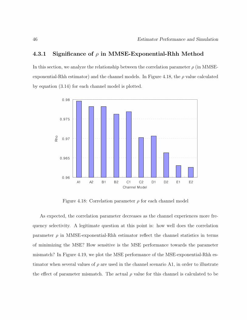
4.3.1 Significance of ρ in MMSE-Exponential-Rhh Method
In this section, we analyze the relationship between the correlation parameter ρ (in MMSE-
exponential-Rhh estimator) and the channel models. In Figure 4.18, the ρ value calculated
by equation (3.14) for each channel model is plotted.
0.96
0.965
0.97
0.975
0.98
A1 A2 B1 B2 C1 C2 D1 D2 E1 E2
Channel Model
Rho
Figure 4.18: Correlation parameter ρ for each channel model
As expected, the correlation parameter decreases as the channel experiences more fre-
quency selectivity. A legitimate question at this point is: how well does the correlation
parameter ρ in MMSE-exponential-Rhh estimator reflect the channel statistics in terms
of minimizing the MSE? How sensitive is the MSE performance towards the parameter
mismatch? In Figure 4.19, we plot the MSE performance of the MSE-exponential-Rhh es-
timator when several values of ρ are used in the channel scenario A1, in order to illustrate
the effect of parameter mismatch. The actual ρ value for this channel is calculated to be
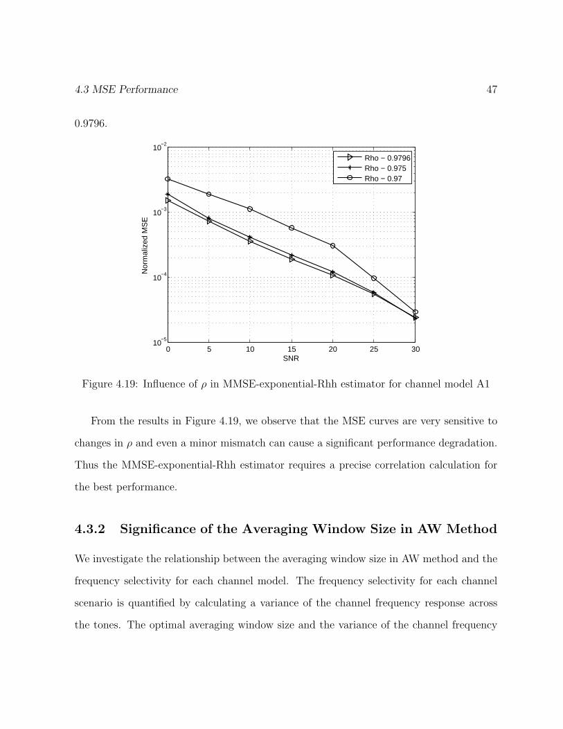
4.3 MSE Performance 47
0.9796.
0 5 10 15 20 25 3010
−5
10−4
10−3
10−2
SNR
Nor
mal
ized
MS
E
Rho − 0.9796Rho − 0.975Rho − 0.97
Figure 4.19: Influence of ρ in MMSE-exponential-Rhh estimator for channel model A1
From the results in Figure 4.19, we observe that the MSE curves are very sensitive to
changes in ρ and even a minor mismatch can cause a significant performance degradation.
Thus the MMSE-exponential-Rhh estimator requires a precise correlation calculation for
the best performance.
4.3.2 Significance of the Averaging Window Size in AW Method
We investigate the relationship between the averaging window size in AW method and the
frequency selectivity for each channel model. The frequency selectivity for each channel
scenario is quantified by calculating a variance of the channel frequency response across
the tones. The optimal averaging window size and the variance of the channel frequency
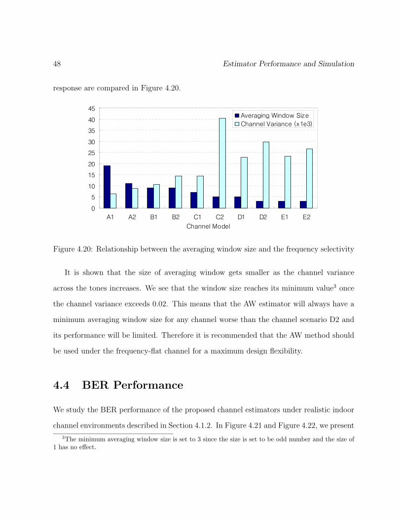
48 Estimator Performance and Simulation
response are compared in Figure 4.20.
0
5
10
15
20
25
30
35
40
45
A1 A2 B1 B2 C1 C2 D1 D2 E1 E2
Channel Model
Averaging Window Size
Channel Variance (x1e3)
Figure 4.20: Relationship between the averaging window size and the frequency selectivity
It is shown that the size of averaging window gets smaller as the channel variance
across the tones increases. We see that the window size reaches its minimum value3 once
the channel variance exceeds 0.02. This means that the AW estimator will always have a
minimum averaging window size for any channel worse than the channel scenario D2 and
its performance will be limited. Therefore it is recommended that the AW method should
be used under the frequency-flat channel for a maximum design flexibility.
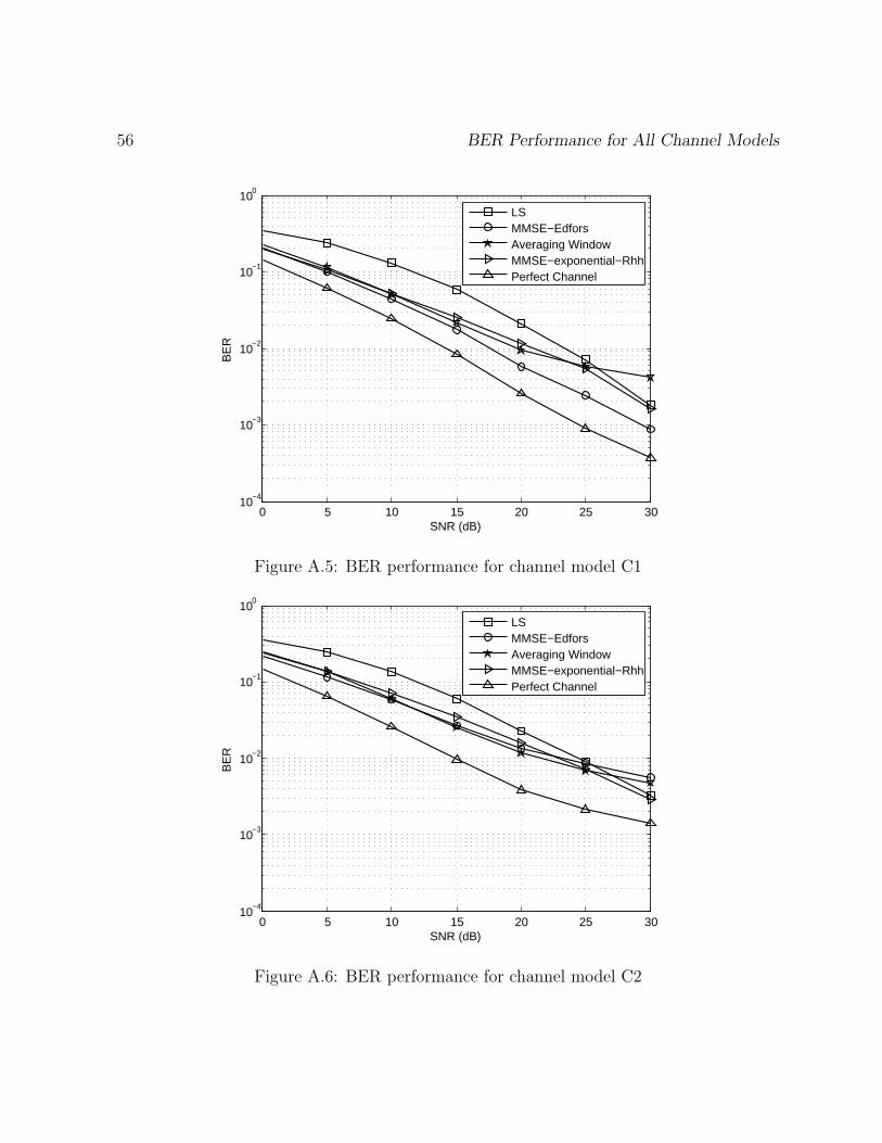
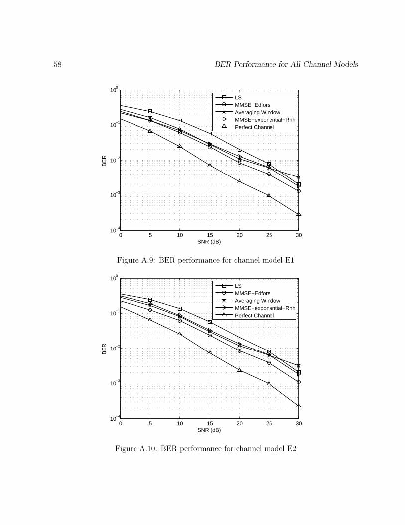
4.4 BER Performance
We study the BER performance of the proposed channel estimators under realistic indoor
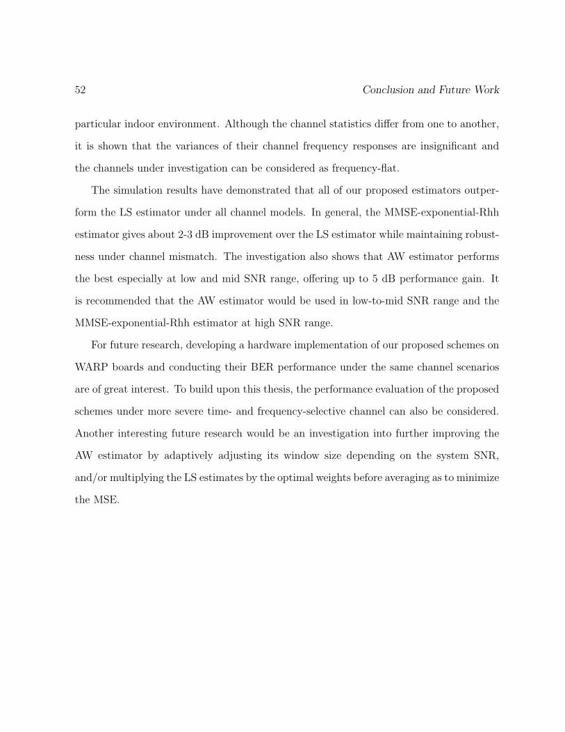
channel environments described in Section 4.1.2. In Figure 4.21 and Figure 4.22, we present
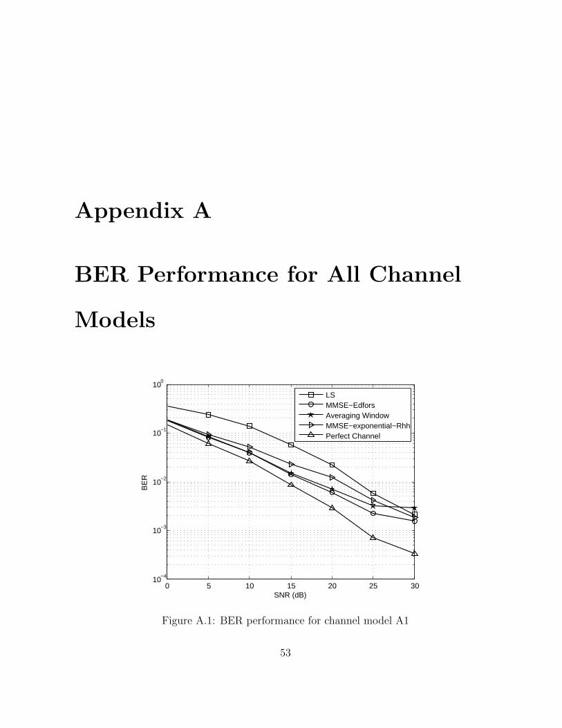
3The minimum averaging window size is set to 3 since the size is set to be odd number and the size of1 has no effect.
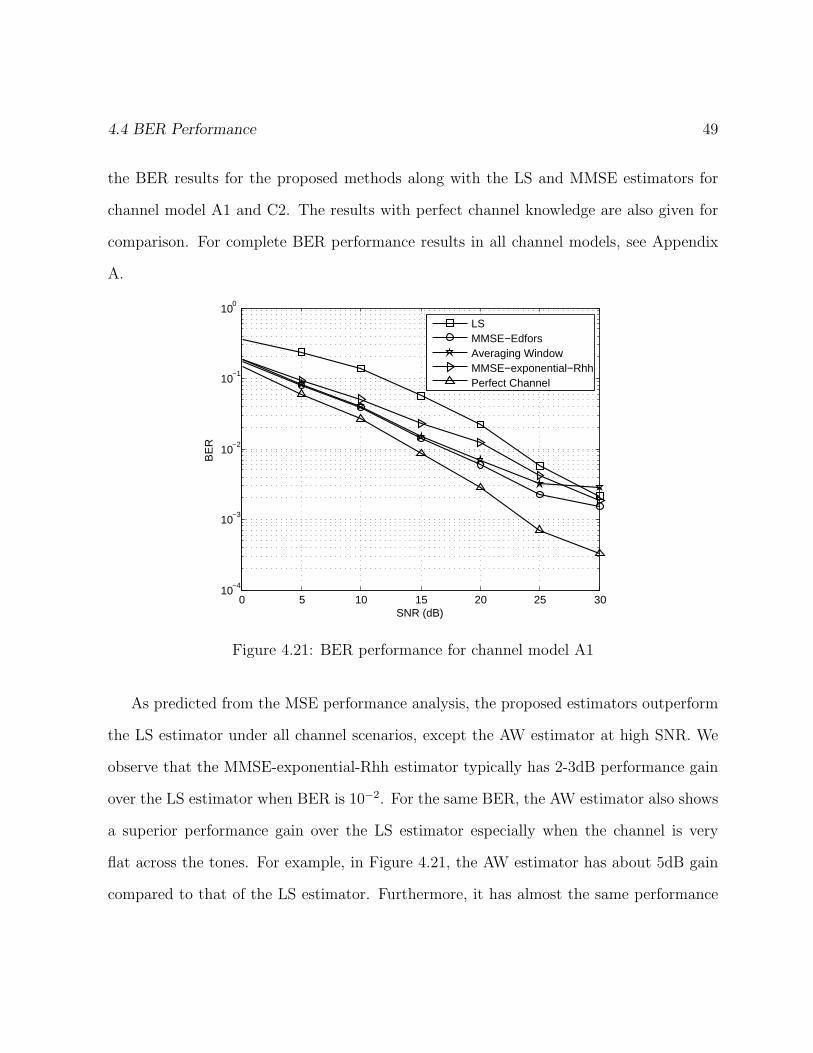
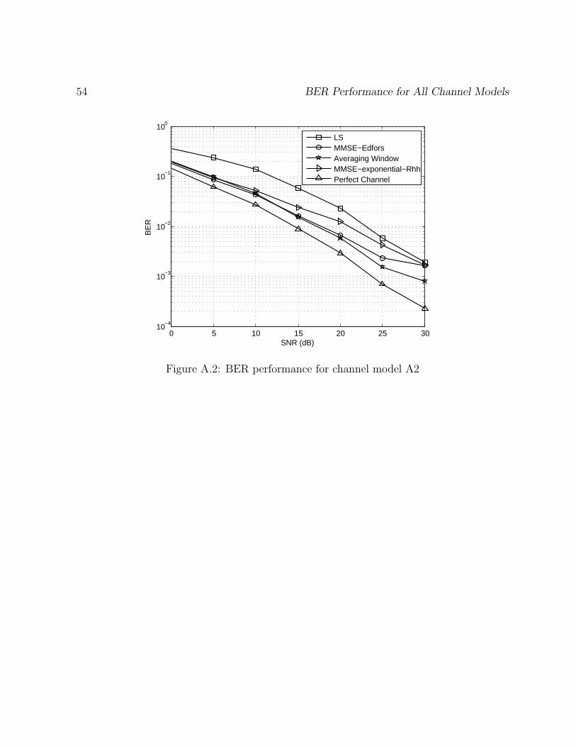
4.4 BER Performance 49
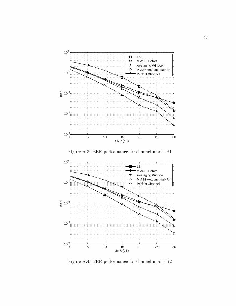
the BER results for the proposed methods along with the LS and MMSE estimators for
channel model A1 and C2. The results with perfect channel knowledge are also given for
comparison. For complete BER performance results in all channel models, see Appendix
A.
0 5 10 15 20 25 3010
−4
10−3
10−2
10−1
100
SNR (dB)
BE
R
LSMMSE−EdforsAveraging WindowMMSE−exponential−RhhPerfect Channel
Figure 4.21: BER performance for channel model A1
As predicted from the MSE performance analysis, the proposed estimators outperform
the LS estimator under all channel scenarios, except the AW estimator at high SNR. We
observe that the MMSE-exponential-Rhh estimator typically has 2-3dB performance gain
over the LS estimator when BER is 10−2. For the same BER, the AW estimator also shows
a superior performance gain over the LS estimator especially when the channel is very
flat across the tones. For example, in Figure 4.21, the AW estimator has about 5dB gain
compared to that of the LS estimator. Furthermore, it has almost the same performance
50 Estimator Performance and Simulation
0 5 10 15 20 25 3010
−4
10−3
10−2
10−1
100
SNR (dB)
BE
R
LSMMSE−EdforsAveraging WindowMMSE−exponential−RhhPerfect Channel
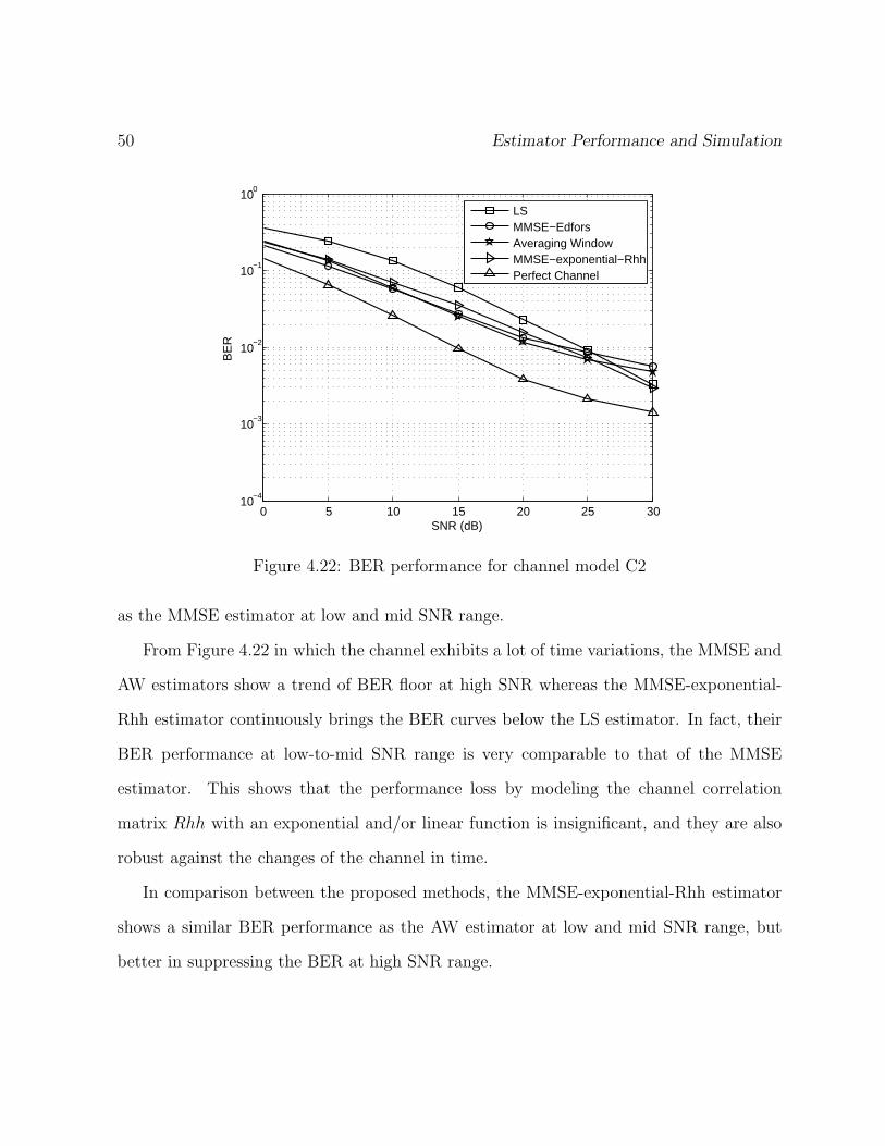
Figure 4.22: BER performance for channel model C2
as the MMSE estimator at low and mid SNR range.
From Figure 4.22 in which the channel exhibits a lot of time variations, the MMSE and
AW estimators show a trend of BER floor at high SNR whereas the MMSE-exponential-
Rhh estimator continuously brings the BER curves below the LS estimator. In fact, their
BER performance at low-to-mid SNR range is very comparable to that of the MMSE
estimator. This shows that the performance loss by modeling the channel correlation
matrix Rhh with an exponential and/or linear function is insignificant, and they are also
robust against the changes of the channel in time.
In comparison between the proposed methods, the MMSE-exponential-Rhh estimator
shows a similar BER performance as the AW estimator at low and mid SNR range, but
better in suppressing the BER at high SNR range.

Chapter 5
Conclusion and Future Work
With ever-increasing interest in OFDM and its adoption in many wireless communication
systems such as the IEEE 802.11, channel estimation becomes one of the most essential
tasks in compensating distortion from the channel. Although active investigation in this
area has resulted in a variety of research, there has been very little effort in understanding
typical indoor environments and designing channel estimation schemes that are both robust
and practical for such channel conditions.
In this work, we have proposed two simple channel estimation techniques: MMSE-
exponential-Rhh that is based on the traditional MMSE estimator with the channel corre-
lation matrix modeled by exponential function, and AW estimator which is based on the
sliding window averaging the LS estimate across the frequency tones. We have also mea-
sured the channel frequency responses under 10 different typical indoor channel scenarios
and translated their information into tapped-delayed-line models for simulation purposes.
The channel measurements have shown that the statistics of the channel are affected
not only by the distance between Tx and Rx, but also by the physical orientation of the
51
52 Conclusion and Future Work
particular indoor environment. Although the channel statistics differ from one to another,
it is shown that the variances of their channel frequency responses are insignificant and
the channels under investigation can be considered as frequency-flat.
The simulation results have demonstrated that all of our proposed estimators outper-
form the LS estimator under all channel models. In general, the MMSE-exponential-Rhh
estimator gives about 2-3 dB improvement over the LS estimator while maintaining robust-
ness under channel mismatch. The investigation also shows that AW estimator performs
the best especially at low and mid SNR range, offering up to 5 dB performance gain. It
is recommended that the AW estimator would be used in low-to-mid SNR range and the
MMSE-exponential-Rhh estimator at high SNR range.
For future research, developing a hardware implementation of our proposed schemes on
WARP boards and conducting their BER performance under the same channel scenarios
are of great interest. To build upon this thesis, the performance evaluation of the proposed
schemes under more severe time- and frequency-selective channel can also be considered.
Another interesting future research would be an investigation into further improving the
AW estimator by adaptively adjusting its window size depending on the system SNR,
and/or multiplying the LS estimates by the optimal weights before averaging as to minimize
the MSE.
Appendix A
BER Performance for All Channel
Models
0 5 10 15 20 25 3010
−4
10−3
10−2
10−1
100
SNR (dB)
BE
R
LSMMSE−EdforsAveraging WindowMMSE−exponential−RhhPerfect Channel
Figure A.1: BER performance for channel model A1
53
54 BER Performance for All Channel Models
0 5 10 15 20 25 3010
−4
10−3
10−2
10−1
100
SNR (dB)
BE
R
LSMMSE−EdforsAveraging WindowMMSE−exponential−RhhPerfect Channel
Figure A.2: BER performance for channel model A2
55
0 5 10 15 20 25 3010
−4
10−3
10−2
10−1
100
SNR (dB)
BE
R
LSMMSE−EdforsAveraging WindowMMSE−exponential−RhhPerfect Channel
Figure A.3: BER performance for channel model B1
0 5 10 15 20 25 3010
−4
10−3
10−2
10−1
100
SNR (dB)
BE
R
LSMMSE−EdforsAveraging WindowMMSE−exponential−RhhPerfect Channel
Figure A.4: BER performance for channel model B2
56 BER Performance for All Channel Models
0 5 10 15 20 25 3010
−4
10−3
10−2
10−1
100
SNR (dB)
BE
R
LSMMSE−EdforsAveraging WindowMMSE−exponential−RhhPerfect Channel
Figure A.5: BER performance for channel model C1
0 5 10 15 20 25 3010
−4
10−3
10−2
10−1
100
SNR (dB)
BE
R
LSMMSE−EdforsAveraging WindowMMSE−exponential−RhhPerfect Channel
Figure A.6: BER performance for channel model C2

57
0 5 10 15 20 25 3010
−4
10−3
10−2
10−1
100
SNR (dB)
BE
R
LSMMSE−EdforsAveraging WindowMMSE−exponential−RhhPerfect Channel
Figure A.7: BER performance for channel model D1
0 5 10 15 20 25 3010
−4
10−3
10−2
10−1
100
SNR (dB)
BE
R
LSMMSE−EdforsAveraging WindowMMSE−exponential−RhhPerfect Channel
Figure A.8: BER performance for channel model D2
58 BER Performance for All Channel Models
0 5 10 15 20 25 3010
−4
10−3
10−2
10−1
100
SNR (dB)
BE
R
LSMMSE−EdforsAveraging WindowMMSE−exponential−RhhPerfect Channel
Figure A.9: BER performance for channel model E1
0 5 10 15 20 25 3010
−4
10−3
10−2
10−1
100
SNR (dB)
BE
R
LSMMSE−EdforsAveraging WindowMMSE−exponential−RhhPerfect Channel
Figure A.10: BER performance for channel model E2
References
[1] IEEE Standard 802.11a 1999. Wireless LAN Medium Access Control (MAC) and
Physical Layer (PHY) Specifications: High-speed Physical Layer in the 5GHz Band.
IEEE, September 1999.
[2] IEEE Standard 802.11b 1999. Wireless LAN Medium Access Control (MAC) and
Physical Layer (PHY) Specifications: High-speed Physical Layer in the 2.4GHz Band.
IEEE, September 1999.
[3] IEEE Standard 802.11g 2003. Wireless LAN Medium Access Control (MAC) and
Physical Layer (PHY) Specifications: Future Higher Data Rate Extension in the 2.4
GHz Band. IEEE, September 2003.
[4] IEEE Standard 802.11nD2.00 2007. Wireless LAN Medium Access Control (MAC) and
Physical Layer (PHY) Specifications: Enhancements for Higher Throughput. IEEE,
September 2007.
[5] IEEE Standard 802.16e 2005. Local and Metropolitan Area Networks - Part 16, Air
Interface for Fixed Broadband Wireless Access Systems. IEEE, September 2005.
59
60 BER Performance for All Channel Models
[6] R. Zhang A. P. Petropulu and R. Lin. Blind ofdm channel estimation through simple
linear precoding. IEEE Trans. Wireless Commun., 3(2):647–655, Mar. 2004.
[7] C. R. N. Athaudage and A. D. S. Jayalath. Enhanced mmse channel estimation using
timing error statistics for wireless ofdm systems. IEEE Trans. Broadcast., 50(4), Dec.
2004.
[8] X. You J. Wang B. Han, X. Gao and E. Costa. An iterative joint channel estimation
and symbol detection algorithm applied in OFDM system with high data to pilot power
ratio. In Proc. IEEE Int’l. Conf. Commun., volume 3, pages 2076–2080, Anchorage,
AK, May 2003.
[9] L. Hanzo B. J. Choi, T. Keller and M. Munster. OFDM and MC-CDMA for Broadband
Multi-User Communications, WLANs and Broadcasting. Wiley-IEEE Press, Aug.
2003.
[10] N. C. Beaulieu C. C. Tan. On first-order markov modeling for the rayleigh fading
channel. IEEE Trans. Commun., 48(12), Dec. 2000.
[11] X. Cai and A. N. Akansu. A subspace method for blind channel identification in
OFDM systems. In Proc. ICC, pages 929–933, New Orleans, LA, Jul. 2000.
[12] J. Cho. A novel channel estimation method for ofdm in high-speed mobile system. In
Proc. IEEE Int’l. Symp.Ind. Electron., volume 1, pages 571–74, Pusan, Korea, Jun.
2001.
[13] R. H. Clarke. A statistical theory of mobile-radio reception. In Bell Syst. Tech. J.,
volume 47, pages 957–1000, 1968.
61
[14] G. Matz D. Schafhuber and F. Hlawatsch. Adaptive wiener filters for time-varying
channel estimation in wireless OFDM systems. In Proc. IEEE Int’l Conf. Acoust.,
Speech, and Signal Processing, volume 4, pages 688–91, Hong Kong, China, Apr.
2003.
[15] J. Cardoso E. Moulines, P. Duhamel and S. Mayrargue. Subspace methods for the
blind identification of multichannel fir filters. IEEE Trans. Signal Process., 43(2):516–
525, Feb. 1995.
[16] M. Engels. Wireless OFDM Systems: How to Make Them Work? Kluwer Academic
Publishers, 2002.
[17] S. W. McLanughln Y. Li M. A. Ingram G. L. Stuber, J. R. Barry and T. G. Pratt.
Broadband mimo-ofdm wireless communications. Proceedings of the IEEE, 92(2), Feb.
2004.
[18] F. Gao and A. Nallanathan. Blind channel estimation for ofdm systems via a gener-
alized precoding. IEEE Trans. Vehicular Technol., 56(3):1155–1164, May 2007.
[19] R. W. Heath and G. B. Giannakis. Exploiting input cyclostationarity for blind channel
identification in ofdm systems. IEEE Trans. Signal Process., 47:848–856, Mar 1999.
[20] M. Hsieh and C. Wei. Channel estimation for ofdm systems based on comb-type pilot
arrangement in frequency selective fading channels. IEEE Trans. Consumer Electron.,
44(1), Feb. 1998.
[21] Eur. Telecommun. Stand. Inst. Broadband Radio Access Networks (BRAN): High
62 BER Performance for All Channel Models
Performance Radio Local Area Networks (HYPERLAN), Type 2; Systems Overview.
ETR 101 683 114, 1999.
[22] M. Sandell S. K. Wilson J. J. van de Beek, O. Edfors and P. O. Borjesson. On channel
estimation in OFDM systems. In Proc. IEEE Vehicular Technology Conf., volume 2,
pages 815–819, Chicago, IL., July 1995.
[23] P. Schramm H. Asplund J. Medbo, H. Andersson and J. E. Berg. Channel models
for hiperlan/2 in different indoor scenarios. Technical report, COST 259 TD(98)070,
1998.
[24] Z. Jianhua and Z. Ping. An improved 2-dimensional pilot-symbols assisted channel
estimation in OFDM systems. In Proc. IEEE Vehicular Technology Conf., volume 3,
pages 1595–99, Jeju, Korea, Apr. 2003.
[25] J. G. Kemeny and J. L. Snell. Finite Markov Chains. Princeton, NJ: Van Nostrand,
1960.
[26] I. Koffman and V. Roman. Broadband wireless access solutions based on ofdm access
in ieee 802.16. EEE Commun. Mag., 51(6):96–103, June 2002.
[27] A. F. Kurpiers. Improved channel estimation and demodulation for OFDM on Hf
ionospheric channels. In Proc. IEEE Int’l Conf. HF radio systems and techniques,
volume 1, pages 65–69, Guildford, UK, Jul. 2000.
[28] C. Li and S. Roy. Subspace-based blind channel estimation for ofdm by exploiting
virtual carriers. IEEE Trans. Wireless Commun., 2(1), Jan. 2003.

63
[29] C. Li and S. Roy. Subspace-based blind channel estimation for ofdm by exploiting
virtural carriers. IEEE Trans. Wireless Commun., 2(1):141–150, Jan. 2003.
[30] D. Lowe and X. Huang. Adaptive low-complexity MMSe channel estimation for
OFDM. In Proc. ISCIT, pages 638–643, Sept. 2006.
[31] ITU-R Recommendation M.1225. Guidelines for evaluation of radio transmission
technologies for IMT-2000. 1997.
[32] H. H. Mmimy. Channel estimation based on coded pilot for OFDM. In Proc. IEEE
Vehic. Tech. Conf., volume 3, pages 1375–79, Phoenix, AZ, May 1997.
[33] B. Muquet and M. de Courville. Blind and semi-blind channel identification methods
using second order statistics for OFDM systems. In Proc. SPAWC, volume 5, pages
170–173, Annapolis, MD, May 1999.
[34] J. J. van de Beek S. K. Wilson O. Edfors, M. Sandell and P. O. Borjesson. Ofdm
channel estimation by singular value decomposition. IEEE Trans. Commun., 46(7),
July 1998.
[35] M. K. Ozdemir and H. Arslan. Channel estimation for wireless ofdm systems. IEEE
Commun. Surveys Tutorials, 9(2), 2007.
[36] A. P. Petropulu and R. Zhang. Blind channel estimation for OFDM systems. In Proc.
DSP/SPE, Atlanta, GA, pages 366–370, Oct. 2002.
[37] J. Proakis. Digital Communications. McGraw-Hill, 1989.
64 BER Performance for All Channel Models
[38] J. Ran E. Bolinth R. Grunheid, H. Rohling and R. Kern. Robust channel estimation
in wireless LANs for mobile environments. In Proc. IEEE Vehicular Technology Conf.
VTC 2002, volume 3, pages 1545–1549, Sept. 2002.
[39] M. Ergen S. Coleri and A. Bahai. Channel estimation techniques based on pilot
arrangement in ofdm systems. IEEE Trans. Broadcast., 48(3):223–229, Sept. 2002.
[40] B. Muquet S. Zhou and G. B. Giannakis. Subspace-based (semi-) blind channel esti-
mation for block precoded space-time ofdm. IEEE Trans. Signal Process., 50(5):1215–
1228, May 2002.
[41] L. L. Scharf. Statistical Signal Processing: Detection, Estimation, and Time Series
Analysis. Reading, MA: Addison-Wesley, 1991.
[42] Y. Shen and E. Martinez. Channel estimation in ofdm systems. Technical Report
AN3059, Freescale Semiconductor, Inc., 2006.
[43] R. Steele. Mobile Radio Communications. New York: Wiley, 1974.
[44] P. Strobach. Bi-iteration svd subspace tracking algorithms. IEEE Trans. Signal Pro-
cessing, 45(5):1222–40, May 1996.
[45] L. Tong and S. Perreau. Multichannel blind identification: From subspace to maximum
likelihood methods. In Proc. IEEE, volume 86, pages 1951–1968, Oct. 1998.
[46] P. Kyritsi A. Molisch D. S. Baum A. Y. Gorokhov C. Oestges Q. Li K. Yu N. Tal B.
D. Dijkstra A. Jagannatham C. Lanzl V. J. Rhodes J. Medbo D. Michelson V. Erceg,
L. Schumacher and M. Webster. TGn Channel Models. May 2004.

65
[47] K. H. Paik W. G. Jeon and Y. S. Cho. An efficient channel estimation technique
for OFDM systems with transmitter diversity. In Proc. IEEE Int’l. Symp. Personal,
Indoor and Mobile Radio Commun., volume 2, pages 1246–1250, London, UK, Sept.
2000.
[48] H. S. Wang and P. C. Chang. On verifying the first-order markovian assumption for
a rayleigh fading channel model. IEEE Trans. Vehicular Technol., 45(2), May 1996.
[49] J. Wu and W. Wu. A comparative study of robust channel estimations for OFDM
system. In Proc. ICCT, pages 1932–1935, 2003.
[50] S. Wu and Y. Bar-Ness. OFDM channel estimation in the presence of frequency offset
and phase noise. In Proc. IEEE Int’l. Conf. Commun., pages 3366–70, May 2003.
[51] Z. Ding X. Zhuang and A. L. Swindlehurst. A statistical subspace method for blind
channel identification in OFDM communications. In Proc. ICASSP, volume 5, pages
2493–2496, 2000.
[52] L. J. Cimini Y. Li and N. R. Sollenberger. Robust channel estimation for ofdm systems
with rapid dispersive fading channels. IEEE Trans. Commun., 46(7), July 1998.
[53] S. Roy Y. Song and L. A. Akers. Joint blind estimation of channel and data symbols
in OFDM. In Proc. IEEE VTC 2000, volume 1, pages 46–50, Tokyo, 2000.
[54] R. Zhang. Blind OFDM channel estimation through linear precoding: A subspace
approach. In Proc. 36th Asilomar Conf., Pacific Grove, CA., pages 631–633, Nov.
2002.