Embed Size (px)
Citation preview
Change Points in Affine Term-StructureModels: Pricing, Estimation and
Forecasting∗
Siddhartha Chib†
Kyu Ho Kang‡
(Washington University in St. Louis)
April 2009, October 2009
Abstract
In this paper we theoretically and empirically examine structural changes in adynamic term-structure model of zero-coupon bond yields. To do this, we de-velop a new arbitrage-free one latent and two macro-economics factor affine modelto price default-free bonds when all model parameters are subject to change atunknown time points. The bonds in our set-up can be priced straightforwardlyonce the change point model is formulated in the manner of Chib (1998) as aspecific unidirectional Markov process. We consider five versions of our generalmodel - with 0, 1, 2, 3 and 4 change points - to a collection of 16 yields measuredquarterly over the period 1972:I to 2007:IV. Our empirical approach to inferenceis fully Bayesian with priors set up to reflect the assumption of a positive term-premium. The use of Bayesian techniques is particularly relevant because themodels are high-dimensional and non-linear, and because it is more straightfor-ward to compare our different change point models from the Bayesian perspective.Our estimation results indicate that the model with 3 change points is most sup-ported by the data and that the breaks occurred in 1980:II, 1985:IV and 1995:II.These dates correspond (in turn) to the time of a change in monetary policy, theonset of what is termed the great moderation, and the start of technology drivenperiod of economic growth. We also utilize the Bayesian framework to derive the
∗We thank Taeyoung Doh, Ed Greenberg, Wolfgang Lemke, Hong Liu, James Morley, SrikanthRamamurthy, Myung Hwan Seo, Yongs Shin, Guofu Zhou, the participants of the 2009 EconometricSociety summer meeting, the 2009 Seminar on Bayesian Inference in Econometrics and Statistics, andthe 2009 Midwest Econometrics Group meeting, and the referees and the Associate editor of this journal,for their thoughtful and useful comments on the paper. Kang acknowledges support from the Center forResearch in Economics and Strategy at the Olin Business School, Washington University in St. Louis.†Address for correspondence: Olin Business School, Washington University in St. Louis, Campus
Box 1133, 1 Bookings Drive, St. Louis, MO 63130. E-mail: [email protected].‡Address for correspondence: Department of Economics, Washington University in St. Louis, Cam-
pus Box 1208, 1 Bookings Drive, St. Louis, MO 63130. E-mail: [email protected].
1

out-of-sample predictive densities of the term-structure. We find that the fore-casting performance of the 3 change point model is substantially better than thatof the other models we examine. (JEL G12, C11, E43)
1 Introduction
In this paper we theoretically and empirically examine structural changes in a dynamic
term-structure model of zero-coupon bond yields. We do our analysis in the setting of
arbitrage-free multi-factor affine models of the type developed in Duffie and Kan (1996)
and Dai and Singleton (2000) though we allow for both latent and macro-economic
factors along the lines of Ang and Piazzesi (2003), Ang, Dong, and Piazzesi (2007) and
Chib and Ergashev (2009). We depart from the existing modeling of structural changes,
however, by relying on a change point process rather than the Markov switching process
of Dai, Singleton, and Yang (2007), Bansal and Zhou (2002), and Ang, Bekaert, and
Wei (2008).
The model we develop and estimate provides a new perspective on the dynamics of
zero-coupon bond prices and yields. One reason is because our change-point approach
reflects a different view of regime-changes. In a change point specification, a regime once
occupied and vacated is never visited again. In contrast, in a Markov switching model,
the regimes recur, which implies that a regime occupied in the past (whether distant or
near) can occur in the future. The latter assumption may not be germane if one believes
that the confluence of conditions that determine a regime are unique and not repeated.
Another reason is because we derive bond prices under the assumption that all pa-
rameters in the model can change whereas in previous work some parameters are assumed
to be constant across regimes. Thus, in our formulation, we do not have to decide which
parameters are constant and which break. As we show, bond prices can be obtained
straightforwardly once the change point process is formulated in the manner of Chib
(1998) as a specific unidirectional Markov process.
A third reason is because in our empirical analysis we deal with a larger set of
maturities than in previous work. This allows us to get finer view of the term-structure
than is possible with a smaller set of maturities. In particular, we apply our model to 16
yields of US T-bills measured quarterly between 1972:I and 2007:IV. An added benefit
of working with these many yields is that (in comparison with models with fewer yields)
the model with 16 yields produces the best forecasts of the term-structure. The reason
for this, which apparently has not been documented or exploited before, is that the
addition of new yields introduces only the parameters that represent the pricing error
variances, but because the parameters are subject to several cross-equation restrictions,
the additional outcomes are helpful in estimation and, hence, in predictive inferences.
A notable aspect of our approach is that the prior distribution is motivated by
economic considerations. In particular, our prior on the parameters reflects the assump-
tion of a positive term-premium, following Chib and Ergashev (2009). Another aspect
is that our estimation approach which is implemented by tuned Markov chain Monte
Carlo methods, is both feasible and reliable. We apply this approach successfully to fit
a model that has 209 parameters. Models of this size in this context would be difficult
to fit by non-Bayesian methods because of the severe non-linearities and the potential
multi-modality of the likelihood function. Our Bayesian approach is also relevant in this
context because it offers a straightforward way to compare different change point models
through marginal likelihoods and Bayes factors.
Our empirical analysis is organized around 5 different versions of the general model.
These models, which we label as M0, M1, M2, M3 and M4, contain 0, 1, 2, 3 and
4 change-points, respectively. Our main findings are as follows. The 3 change point
model, M3, is the one that is most supported by the data (in comparison with models
with 0, 1, 2 and 4 change-points) and that the breaks occurred in 1980:II, 1985:IV and
1995:II. These change-points can be attributed, in turn, to changes in monetary policy,
the onset of what is termed the great moderation, and the start of the technology driven
period of economic growth. Thus, the most recent break occurs in 1995, not 1985, as is
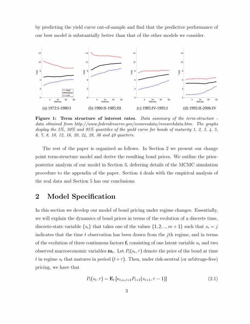
commonly believed. That the underlying distribution of the term-structure is different in
the regimes isolated by these change-points can be seen in Figure 1 where we display the
5%, 50% and 95% quantiles of the yield curve data categorized by regime. As we discus
below, the model estimation reveals that the parameters across regimes are substantially
different, which provides support to our approach of letting all the parameters vary
across regimes. We find, for instance, that the mean-reversion parameters in the factor
dynamics and the factor loadings are regime-specific. We conclude our empirical analysis
2
by predicting the yield curve out-of-sample and find that the predictive performance of
our best model is substantially better than that of the other models we consider.
4 24 40 600
3
6
9
12
15
Maturity
Yie
ld
HighMedianLow
4 24 40 600
3
6
9
12
15
Maturity
Yie
ld
4 24 40 600
3
6
9
12
15
Maturity
Yie
ld
4 24 40 600
3
6
9
12
15
Maturity
Yie
ld
(a) 1972:I-1980:I (b) 1980:II-1985:III (c) 1985:IV-1995:I (d) 1995:II-2006:IV
Figure 1: Term structure of interest rates. Data summary of the term-structure -data obtained from http://www.federalreserve.gov/econresdata/researchdata.htm. The graphsdisplay the 5%, 50% and 95% quantiles of the yield curve for bonds of maturity 1, 2, 3, 4, 5,6, 7, 8, 10, 12, 16, 20, 24, 28, 36 and 40 quarters.
The rest of the paper is organized as follows. In Section 2 we present our change
point term-structure model and derive the resulting bond prices. We outline the prior-
posterior analysis of our model in Section 3, deferring details of the MCMC simulation
procedure to the appendix of the paper. Section 4 deals with the empirical analysis of
the real data and Section 5 has our conclusions.
2 Model Specification
In this section we develop our model of bond pricing under regime changes. Essentially,
we will explain the dynamics of bond prices in terms of the evolution of a discrete time,
discrete-state variable st that takes one of the values 1, 2, ..,m+ 1 such that st = j
indicates that the time t observation has been drawn from the jth regime, and in terms
of the evolution of three continuous factors ft consisting of one latent variable ut and two
observed macroeconomic variables mt. Let Pt(st, τ) denote the price of the bond at time
t in regime st that matures in period (t+τ). Then, under risk-neutral (or arbitrage-free)
pricing, we have that
Pt(st, τ) = Et [κt,st,t+1Pt+1(st+1, τ − 1)] (2.1)
3

where Et is the expectation over (ft+1, st+1), conditioned on (ft, st), under the physical
measure, and κt,st,t+1 is the stochastic discount factor (SDF) that converts a time (t+ 1)
payoff into a payoff at time t in regime st.
Our goal now is to characterize the stochastic evolution of st and the factors ft and
describe our model of the SDF κt,st,t+1 in terms of the short-rate process and the market
price of factor risks. Given these ingredients, we then derive the prices of our default-free
zero coupon bonds that satisfy the preceding condition.
2.1 Change Point Process
We assume that the process of regime-changes is governed by st ∈ 1, 2, ...,m + 1.When st = j, the tth observation is assumed to be drawn from regime j. We refer to
the times t1, t2, ..., tm at which st jumps from one value to the next as the change-
points. We will suppose that the parameters in the (m + 1) regimes induced by these
m change-points are different. As mentioned in Section 1, we describe the stochastic
evolution of st in terms of a change point instead of a Markov switching process. In
this we follow Chib (1998). We suppose that from one time period to the next st can
either stay at the current value j or jump to the next higher value (j + 1). In this sense
st can be viewed as a unidirectional process. Thus, in this formulation, return visits
to a previously occupied state are not possible. Then, it follows that the jth change
point occurs at time (say) tj when stj−1 = j and stj = j + 1 (j = 1, 2, ..,m). We further
assume that st follows a Markov process with transition probabilities given by
P =
p11 1− p11 0 · · · 00 p22 1− p22 · · · 00 0 p33 0...
.... . .
0 0 0 pm+1,m+1
(2.2)
where pjk = Pr[st+1 = k|st = j] and, pjk = 1 − pjj, k = j + 1 and pm+1,m+1 = 1
(j = 1, 2, ..,m).
A feature of this specification is an absorbing terminal state. This is intentional
because in any setting with a finite observation window one must have an upper limit on
the number of change-points (equivalently, the number of possible regimes). An upper
limit on the number of change-points does not rule out, however, the possibility of breaks
4
beyond the observation window. Although such breaks can occur it is not possible to
make inferences about them from the sample data without making consequential and
unverifiable assumptions.
An interesting point is that we can assume that the (infinitely lived) economic agents
face a possible infinity of change-points. Regardless of the number of change points,
however, as is typical in finance and economic theorizing, we assume that these agents
know the parameters in the various regimes. Furthermore, in the asset pricing context,
we assume that these agents know the current value of the state variable. The central
uncertainty from the perspective of these agents is that the state of the next period is
random - either the current regime continues or the next possible regime emerges.
This formulation of the change point model in terms of a restricted unidirectional
Markov process facilitates bond pricing (as we show below). It also makes obvious
how the change point assumption differs from the Markov-switching regime process in
Dai et al. (2007), Bansal and Zhou (2002) and Ang et al. (2008) where the transition
probability matrix is unrestricted and previously occupied states can be revisited. As
we have argued above, there are strong reasons for looking at the term structure from
the change point perspective.
2.2 Factor Process
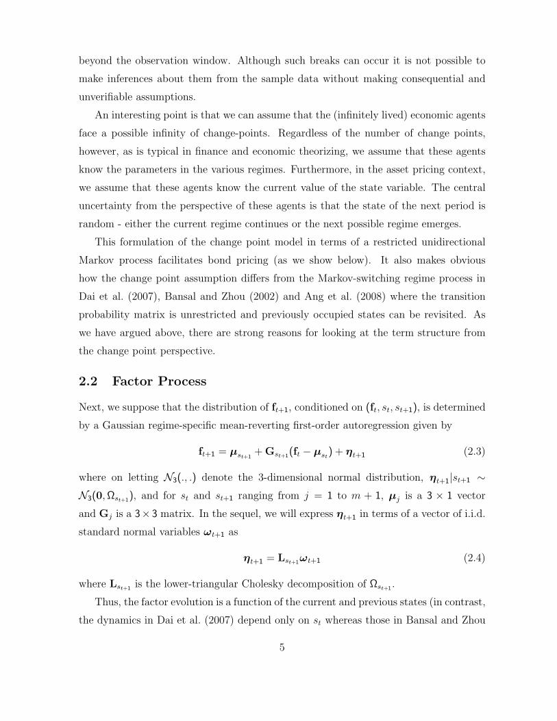
Next, we suppose that the distribution of ft+1, conditioned on (ft, st, st+1), is determined
by a Gaussian regime-specific mean-reverting first-order autoregression given by
ft+1 = µst+1+ Gst+1(ft − µst
) + ηt+1 (2.3)
where on letting N3(., .) denote the 3-dimensional normal distribution, ηt+1|st+1 ∼N3(0,Ωst+1), and for st and st+1 ranging from j = 1 to m + 1, µj is a 3 × 1 vector
and Gj is a 3× 3 matrix. In the sequel, we will express ηt+1 in terms of a vector of i.i.d.
standard normal variables ωt+1 as
ηt+1 = Lst+1ωt+1 (2.4)
where Lst+1 is the lower-triangular Cholesky decomposition of Ωst+1 .
Thus, the factor evolution is a function of the current and previous states (in contrast,
the dynamics in Dai et al. (2007) depend only on st whereas those in Bansal and Zhou
5
(2002) and Ang et al. (2008) depend only on st+1). This means that the expectation
of ft+1 conditioned on (ft, st = j, st+1 = k) is a function of both µj and µk. The
appearance of µj in this expression is natural because one would like the autoregression
at time (t+ 1) to depend on the deviation of ft from the regime in the previous period.
Of course, the parameter µj can be interpreted as the expectation of ft+1 when regime
j is persistent. The matrices Gj can also be interpreted in the same way as the
mean-reversion parameters in regime j.
2.3 Stochastic Discount Factor
We complete our modeling by assuming that the SDF κt,st,t+1 that converts a time (t+1)
payoff into a payoff at time t in regime st is given by
κt,st,t+1 = exp
(−rt,st −
1
2γ ′t,st
γt,st− γ ′t,st
ωt+1
)(2.5)
where rt,st is the short-rate in regime st, γt,stis the vector of time-varying and regime-
sensitive market prices of factor risks and ωt+1 is the i.i.d. vector of regime independent
factor shocks in (2.4). The SDF is independent of st+1 given st as in the model of Dai
et al. (2007).
We suppose that the short rate is affine in the factors and of the form
rt,st = δ1,st + δ′2,st(ft − µst
) (2.6)
where the intercept δ1,st varies by regime to allow for shifts in the level of the term
structure. The multiplier δ2,st : 3× 1 is also regime-dependent in order to capture shifts
in the effects of the macroeconomic factors on the term structure. This is similar to
the assumption in Bansal and Zhou (2002) but a departure from both Ang et al. (2008)
and Dai et al. (2007) where the coefficient on the factors is constant across regimes.
A consequence of our assumption is that the bond prices that satisfy the risk-neutral
pricing condition can only be obtained approximately. The same difficulty arises in the
work of Bansal and Zhou (2002).
We also assume that the dynamics of γt,stare governed by
γt,st= γst
+ Φst(ft − µst) (2.7)
6

where γst: 3 × 1 is the regime-dependent expectation of γt,st
and Φst : 3 × 3 is a
matrix of regime-specific parameters. We refer to the collection (γst, Φst) as the factor-
risk parameters. Note that in this specification γt,stis the same across maturities but
different across regimes. A point to note is that negative market prices of risk have the
effect of generating a positive term premium. This is important to keep in mind when
we construct the prior distribution on the risk parameters.
It is easily checked that E [κt,st,t+1|ft, st = j] is equal to the price of a zero coupon
bond with τ = 1:
E [κt,st,t+1|ft, st = j] =
j+1∑st+1=j
pjst+1E [κt,st,t+1|ft, st = j, st+1] (2.8)
= exp (−rt,j) , j ∈ 1, 2, ..,m
In other words, the SDF satisfies the intertemporal no-arbitrage condition (Dai et al.
(2007)).
We note that regime-shift risk is equal to zero in our version of the SDF. We make
this assumption because it is difficult to identify this risk from our change-point model
where each regime-shift occurs once. Regime risk cannot also be isolated in the models
of Ang et al. (2008) and Bansal and Zhou (2002) for the reason that it is confounded
with the market price of factor risk.
2.4 Bond Prices
Under these assumptions, we now solve for bond prices that satisfy the risk-nuetral
pricing condition
Pt(st, τ) = Et [κt,st,t+1Pt+1(st+1, τ − 1)] (2.9)
Following Duffie and Kan (1996), we assume that Pt(st, τ) is a regime-dependent expo-
nential affine function of the factors taking the form
Pt(st, τ) = exp(−τRτt) (2.10)
where Rτt is the continuously compounded yield given by
Rτt =1
τast(τ) +
1
τbst(τ)′(ft − µst
) (2.11)
7
and ast(τ) is a scalar function and bst(τ) is a 3× 1 vector of functions, both depending
on st and τ .
We find the expressions for the latter functions by the method of undetermined
coefficients. By the law of the iterated expectation, the risk-neutral pricing formula in
(2.9) can be expressed as
1 = Et
Et,st+1
[κt,st,t+1
Pt+1(st+1, τ − 1)
Pt(st, τ)
](2.12)
where the inside expectation Et,st+1 is conditioned on st+1, st and ft. Subsequently, as
discussed in Appendix A, one now substitutes Pt(st, τ) and Pt+1(st+1, τ − 1) from (2.10)
and (2.11) into this expression, and integrate out st+1 after a log-linearization. We
match common coefficients and solve for the unknown functions. When j ∈ 1, ..,mand k = j + 1, this procedure produces the following recursive system for the unknown
functions
aj(τ) =(pjj pjk
)( δ1,j − γjL′jbj(τ − 1)− bj(τ − 1)′LjL′jbj(τ − 1)/2 + aj(τ − 1)
δ1,j − γjL′kbk(τ − 1)− bk(τ − 1)′LkL′kbk(τ − 1)/2 + ak(τ − 1)
)bj(τ) =
(pjj pjk
)( δ2,j + (Gj − LjΦj)′ bj(τ − 1)
δ2,j + (Gk − LkΦj)′ bk(τ − 1)
)(2.13)
where τ runs over the positive integers. These recursions are initialized by setting
ast(0) = 0 and bst(0) = 03×1 for all st. It is readily seen that the resulting intercept and
factor loadings are determined by the weighted average of the two potential realizations
in the next period where the weights are given by the transition probabilities pjj and
(1 − pjj), respectively. Thus, the bond prices in regime st = j (j ≤ m) incorporate
the expectation that the economy in the next period will continue to stay in regime j,
or that it will switch to the next possible regime k = j + 1, each weighted with the
probabilities pjj and 1− pjj, respectively.
Note that when we consider inference with a given sample of data, and the number
of change points m is a finite number, the above recursions are supplemented by the
expressions
aj(τ) = δ1,j − γjL′jbj(τ − 1)− bj(τ − 1)′LjL′jbj(τ − 1)/2 + aj(τ − 1)
bj(τ) = δ2,j + (Gj − LjΦj)′ bj(τ − 1) (2.14)
for j = m + 1.
8
Θt Θt+1Θt−1
ft+1ftft−1
st−1 st st+1
Rt+1RtRt−1
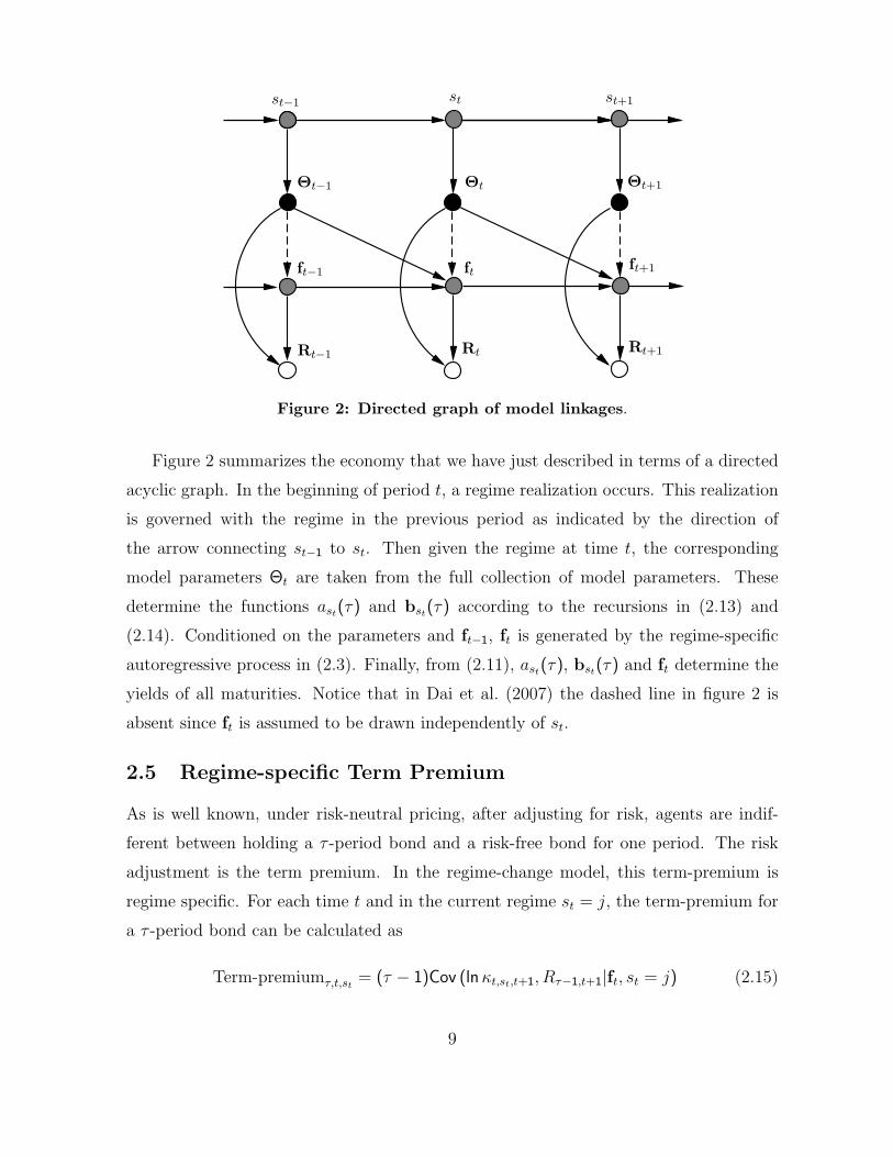
Figure 2: Directed graph of model linkages.
Figure 2 summarizes the economy that we have just described in terms of a directed
acyclic graph. In the beginning of period t, a regime realization occurs. This realization
is governed with the regime in the previous period as indicated by the direction of
the arrow connecting st−1 to st. Then given the regime at time t, the corresponding
model parameters Θt are taken from the full collection of model parameters. These
determine the functions ast(τ) and bst(τ) according to the recursions in (2.13) and
(2.14). Conditioned on the parameters and ft−1, ft is generated by the regime-specific
autoregressive process in (2.3). Finally, from (2.11), ast(τ), bst(τ) and ft determine the
yields of all maturities. Notice that in Dai et al. (2007) the dashed line in figure 2 is
absent since ft is assumed to be drawn independently of st.
2.5 Regime-specific Term Premium
As is well known, under risk-neutral pricing, after adjusting for risk, agents are indif-
ferent between holding a τ -period bond and a risk-free bond for one period. The risk
adjustment is the term premium. In the regime-change model, this term-premium is
regime specific. For each time t and in the current regime st = j, the term-premium for
a τ -period bond can be calculated as
Term-premiumτ,t,st= (τ − 1)Cov (lnκt,st,t+1, Rτ−1,t+1|ft, st = j) (2.15)
9
= −pjjbj(τ − 1)′Ljγt,j − pjkbk(τ − 1)′Lkγt,j
where k = j + 1. One can see that if Lj, which quantifies the size of the factor shocks
in the current regime st = j, is large, or if γt,j, the market prices of factor risk, is highly
negative, then the term premium is expected to be large. Even if Lj in the current
regime is small, one can see from the second term in the above expression that the
term premium can be big if the probability of jumping to the next possible regime is
high and Lk in that regime is large. In our empirical implementation we calculate this
regime-specific term premium for each time period in the sample.
3 Estimation and Inference
In this section we consider the empirical implementation of our yield curve model. In
order to get a detailed perspective of the yield curve and its dynamics over time we
operationalize our pricing model on a data set of 16 yields of US T-bills measured
quarterly between 1972: I and 2007: IV on the maturities given by
1, 2, 3, 4, 5, 6, 7, 8, 10, 12, 16, 20, 24, 28, 36, 40
quarters. As far as we know, this is the largest number of yields that have been considered
in the setting of affine yield curve models. For these data, we consider five versions of
our general model, with 0, 1, 2, 3 and 4 change points and denoted by Mm4m=0.
The largest model that we fit, namely M4, has a total of 209 free parameters. We fit
these various models by tuned Bayesian methods as we discuss below and then compare
the competing models through marginal likelihoods, Bayes factors and the predictive
performance out of sample.
To begin, let the 16 yields under study be denoted by
(R1t, R2t, .., R16t)′ , t = 1, 2, ..., n, (3.1)
where Rit = Rτi,t and τi is the ith maturity (in quarters), and let the two macro factors
be denoted by
mt = (m1t, m2t) , t = 1, 2, ..., n
where m1t is the inflation rate and m2t is the real GDP growth rate. We also let
Sn = stnt=1
10
denote the sequence of (unobserved) regime indicators.
We now specify the set of model parameters to be estimated. First, the unknown
elements of Gst and Φst are denoted by
gst = Gij,sti,j=1,2,3 and φst= Φjj,stj=1,2,3
where Gij,st and Φij,st denote the (i, j)th element of Gst and Φst , respectively. The
unknown elements of Ωst are defined as
λst = l21,st , l∗22,st
, l31,st , l32,st , l∗33,st
where these are obtained from the decomposition Ωst = LstL′st
with Lst expressed as 1/400 0 0l21,st exp(l∗22,st
) 0l31,st l32,st exp(l∗33,st
)
(3.2)
The elements of λst are unrestricted. Next, the parameters of the short-rate equation
are expressed as δst = (δ1,st × 400, δ′2,st)′ and those in the transition matrix P by
p = pjj, j = 1, 2, ..,m. Finally, the unknown pricing error variances σ2i,st
are collected
in reparameterized form as
σ∗2 = σ∗2i,st= diσ
2i,st, i = 1, .., 7, 8, .., 16 and st = 1, 2, ..,m + 1
where d1 = 30, d2 = d16 = 40, d3 = d12 = 200, d4 = 350, d5 = d6 = d11 = 500, d7 = 3000,
d9 = 1500, d10 = 1000, d13 = d14 = d15 = 200. These positive multipliers are introduced
to increase the magnitude of the variances.
Under these notations, for any given model with m change-points, the parameters of
interest can be denoted as ψ = (θ,σ∗2, u0) where
θ = gst , µm,st, δst , γst
, φst, λst , pm+1
st=1
and u0 is the latent factor at time 0. Note that to economize on notation, we do not
index these parameters by a model subscript.
3.1 Joint distribution of the yields and macro factors
We now derive the joint distribution of the yields and the macro factors conditioned on
Sn and ψ. This joint distribution can be obtained without marginalization over utnt=1
11
if we assume (following, for example, Chen and Scott (2003) and Dai et al. (2007)) that
one of the yields is priced exactly without error. This is the so-called basis yield. Under
this assumption the latent factor can be expressed in terms of the observed variables
and eliminated from the model, as we now describe.
Assume that R8t (the eighth yield in the list above) is the basis yield which is priced
exactly by the model. Let Rt denote the remaining 15 yields (which are measured with
pricing error). Define ai,st = ast(τi)/τi and bi,st = bst(τi)/τi where ast(τi) and bst(τi)
are obtained from the recursive equations in (2.13) - (2.14). Also let a8,st (ast) and
b8,st (bst) be the corresponding intercept and factor loadings for R8t (Rt), respectively.
Then, since the basis yield is priced without error, if we let
b8,st =
(b8,u,st
b8,m,st
)(3.3)
we can see from (2.11) that R8t is given by
R8t = a8,st + b8,u,stut + b′8,m,st(mt − µm,st
) (3.4)
On rewriting this expression, it follows that ut is
ut =(b8,u,st
)−1 (R8t − a8,st − b′8,m,st
(mt − µm,st))
(3.5)
Conditioned on mt and st, this represents a one-to-one map between R8t and ut. If we
let
zt =
(R8t
mt
),
αst =
( (b8,u,st
)−1b′8,m,st
µm,st−(b8,u,st
)−1a8,st
02×1
), and (3.6)
Ast =
( (b8,u,st
)−1 −(b8,u,st
)−1b′8,m,st
02×1 I2
)then one can check that ft can be expressed as
ft = αst + Astzt (3.7)
It now follows from equation (2.11) that conditioned on zt (equivalently ft), st and the
model parameters ψ, the non-basis yields Rt in our model are generated according to
the process
Rt = ast + bst(ft − µst) + εt, εt ∼ iidN (0,Σst) (3.8)
12
where
Σst = diag(σ21,st, σ2
2,st, .., σ2
7,st, σ2
9,st, .., σ2
16,st).
In other words,
p(Rt|zt, st,ψ) = p(Rt|ft, st,ψ) (3.9)
= N15(Rt|ast + bst(ft − µst),Σst)
In addition, the distribution of zt conditioned on zt−1, st and st−1 is obtained straight-
forwardly from the process generating ft given in equation (2.3) and the linear map
between ft and zt given in equation (3.7). In particular,
p(zt|zt−1, st, st−1,ψ) = p(ft|ft−1, st, st−1,ψ) det (Ast) (3.10)
= N3(µst+ Gst(ft−1 − µst−1
),Ωst)|(b8,u,st
)−1 |
If we let
yt = (Rt, zt) and y = ytnt=1
it follows that the required joint density of y conditioned on (Sn,ψ) is given by
p(y|Sn,ψ) =n∏t=1
N15(Rt|ast + bst(ft − µst),Σst) (3.11)
×N3(µst+ Gst(ft−1 − µst−1
),Ωst)|(b8,u,st
)−1 | (3.12)
3.2 Prior Distribution
Because of the size of the parameter space, and the complex cross-maturity restrictions
on the parameters, the formulation of the prior distribution can be a challenge. Chib
and Ergashev (2009) have tackled this problem and shown that a reasonable approach
for constructing the prior is to think in terms of the term structure that is implied by the
prior distribution. The implied yield curve can be determined by simulation: simulating
parameters from the prior and simulating yields from the model given the parameters.
The prior can be adjusted until the implied term structure is viewed as satisfactory on
a priori considerations. Chib and Ergashev (2009) use this strategy to arrive at a prior
distribution that incorporates the belief of a positive term premium and stationary but
persistent factors. We adapt their approach for our model with change-points, ensuring
13
that the yield curve implied by our prior distribution is upward sloping. We assume, in
addition, that the prior distribution of the regime specific parameters is identical across
regimes. We arrive at our prior distribution in this way for each of the five models we
consider - with 0, 1, 2, 3 and 4 change-points.
We begin by recalling the identifying restrictions on the parameters. First, we set
µu,st= 0 which implies that the mean of the short rate conditional on st is δ1,st . Next,
the first element of δ2,st , namely δ21,st , is assumed to be non-negative. Finally, to enforce
stationarity of the factor process, we restrict the eigenvalues of Gst to lie inside the unit
circle. Thus, under the physical measure, the factors are mean reverting in each regime.
These constraints are summarized as
R = Gj, δ21,j|δ21,j ≥ 0, 0 ≤ pjj ≤ 1, |eig(Gj)| < 1 for j = 1, 2, ..,m + 1 (3.13)
All the constraints in R are enforced through the prior distribution.
The free parameters in θ and σ∗2 are assumed to be mutually independent. Our prior
distribution on θ is normal N (θ, Vθ) truncated by the restrictions in R. In particular,
the N (θ, Vθ) distribution has the form
m∏st=1
N (pstst |pstst , Vpstst)
×m+1∏st=1
N (gst |gst , Vgst
)N (µm,st|µm,st
, Vµm,st)N (δst |δst , Vδst
)
×m+1∏st=1
N (γst
|γst, Vγst
)N (φst|φst
, Vφst)N (λst |λst , Vλst
)
which we explain as follows.
First, the prior on pjj (j = 1, ..,m) is normal with a standard deviation of 0.33,
truncated to the interval (0, 1). The mean of these distributions is model-specific. For
example, in theM1 model, the mean is 0.986, so that the a priori expected duration of
stay in regime 1 is about 70 quarters in relation to a sample period of 140 quarters. In
theM2, M3 and M4 models, the prior mean of the transition probabilities is specified
to imply 50, 40 and 33 quarters of expected duration in each regime. It is important
to note that we work with a truncated normal prior distribution on these transition
probabilities instead of the more conventional beta distribution because ast and bst in
14

the equation (3.8) are a function of pjj, which eliminates any benefit from the use of a
beta functional form. Second, we construct gst from the matrix
Gst = diag(0.95, 0.8, 0.4)
and let Vgstbe a diagonal matrix with each diagonal element equal to 0.1. This choice of
prior incorporates the prior belief that the latent factor is more persistent than the macro
factors. Third, we assume that µm,st× 400 = (4, 3)′ and Vµm,st
× 4002 = diag(25, 1).
Thus, the prior mean of inflation is assumed to be 4% and that of real GDP growth rate
to be 3%. The standard deviations of 5% and 1% produces a distribution that covers
the most likely values of these rates. Fourth, based on the Taylor rule intuition that
the response of the short rate to an increase of inflation and output growth tend to be
positive, we let
δst = (6, 0.8, 0.4, 0.4)
and the let the prior standard deviations be (5, 0.4, 0.4, 0.4). Fifth, we assume that
γst= (−0.5,−0.5,−0.5) and Vγst
= diag(0.1, 0.1, 0.1)
where the prior mean of γstis negative in order to suggest an upward sloping average
yield curve in each regime. Sixth, we assume that
φst= (1, 1, 1) and Vφst
= diag(1, 1, 1)
where the positive prior is justified from the intuition that positive shocks to macroeco-
nomic fundamentals should tend to decrease the overall risk in the economy. Seventh,
we let
λst = (0, 0, 0, 0, 1) and Vλst= diag(4, 4, 4, 4, 4)
which tends to imply reasonable prior variation in the implied yield curve.
Next, we place the prior on the 15×m free parameters of σ∗2. Each σ∗2i,stis assumed
to have an inverse-gamma prior distribution IG(v, d) with v = 4.08 and d = 20.80 which
implies a mean of 10 and standard deviation of 14.
Finally, we assume that the latent factor u0 at time 0 follows the steady-state distri-
bution in regime 1
u0 ∼ N (0, Vu) (3.14)
15
where Vu =(1−G2
11,1
)−1.
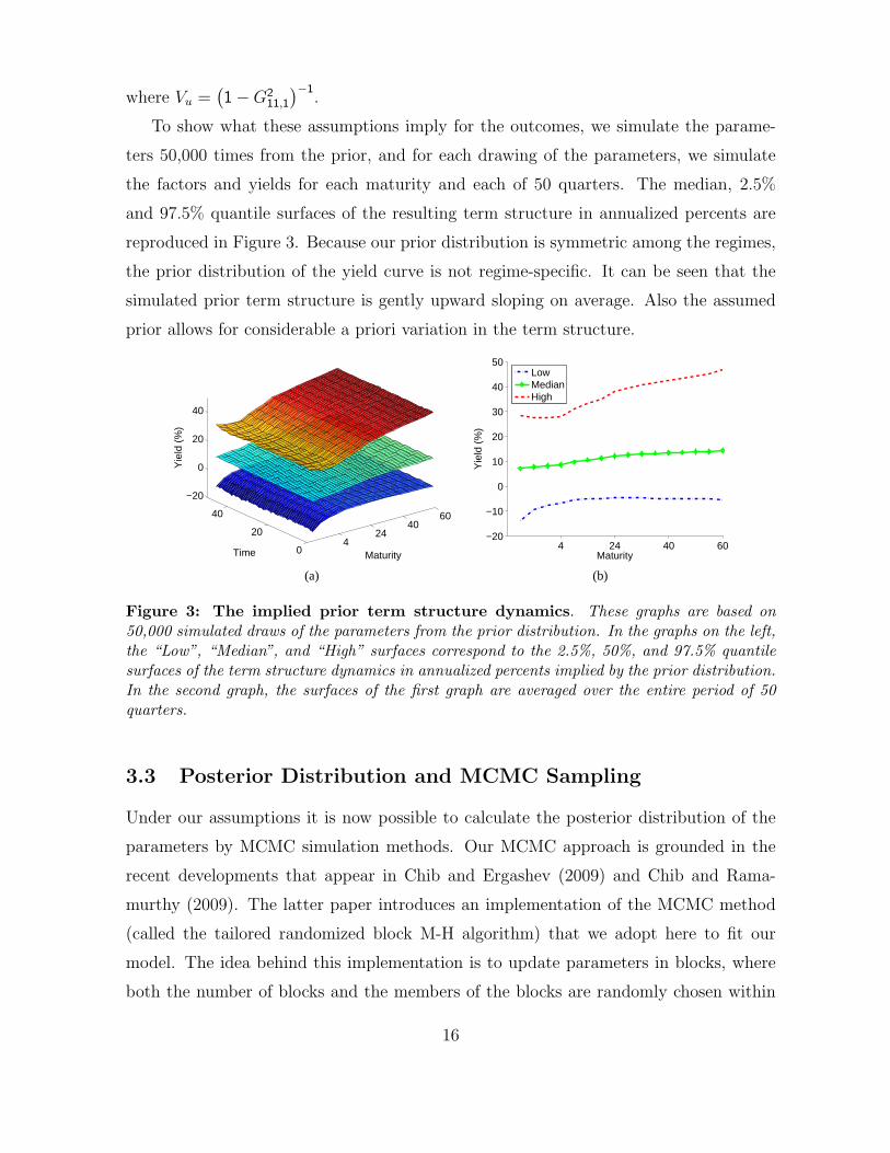
To show what these assumptions imply for the outcomes, we simulate the parame-
ters 50,000 times from the prior, and for each drawing of the parameters, we simulate
the factors and yields for each maturity and each of 50 quarters. The median, 2.5%
and 97.5% quantile surfaces of the resulting term structure in annualized percents are
reproduced in Figure 3. Because our prior distribution is symmetric among the regimes,
the prior distribution of the yield curve is not regime-specific. It can be seen that the
simulated prior term structure is gently upward sloping on average. Also the assumed
prior allows for considerable a priori variation in the term structure.
424
4060
0
20
40
−20
0
20
40
MaturityTime
Yie
ld (
%)
4 24 40 60−20
−10
0
10
20
30
40
50
Maturity
Yie
ld (
%)
LowMedianHigh
(a) (b)
Figure 3: The implied prior term structure dynamics. These graphs are based on50,000 simulated draws of the parameters from the prior distribution. In the graphs on the left,the “Low”, “Median”, and “High” surfaces correspond to the 2.5%, 50%, and 97.5% quantilesurfaces of the term structure dynamics in annualized percents implied by the prior distribution.In the second graph, the surfaces of the first graph are averaged over the entire period of 50quarters.
3.3 Posterior Distribution and MCMC Sampling
Under our assumptions it is now possible to calculate the posterior distribution of the
parameters by MCMC simulation methods. Our MCMC approach is grounded in the
recent developments that appear in Chib and Ergashev (2009) and Chib and Rama-
murthy (2009). The latter paper introduces an implementation of the MCMC method
(called the tailored randomized block M-H algorithm) that we adopt here to fit our
model. The idea behind this implementation is to update parameters in blocks, where
both the number of blocks and the members of the blocks are randomly chosen within
16

each MCMC cycle. This strategy is especially valuable in high-dimensional problems
and in problems where it is difficult to form the blocks on a priori considerations.
The posterior distribution that we would like to explore is given by
π(Sn,ψ|y) ∝ p(y|Sn,ψ)p(Sn|ψ)π(ψ) (3.15)
where p(y|Sn,ψ) is the distribution of the data given the regime indicators and the
parameters, p(Sn|ψ) is the density of the regime-indicators given the parameters and the
initial latent factor, and π(ψ) is the joint prior density of u0 and the parameters. Note
that by conditioning on Sn we avoid the calculation of the likelihood function p(y|ψ)
whose computation is more involved. We discuss the computation of the likelihood
function in the next section in connection with the calculation of the marginal likelihood.
The idea behind the MCMC approach is to sample this posterior distribution iter-
atively, such that the sampled draws form a Markov chain with invariant distribution
given by the target density. Practically, the sampled draws after a suitably specified
burn-in are taken as samples from the posterior density. We construct our MCMC sim-
ulation procedure by sampling various blocks of parameters and latent variables in turn
within each MCMC iteration. The distributions of these various blocks of parameters
are each proportional to the joint posterior π(Sn,ψ|y). In particular, after initializing
the various unknowns, we go through 4 iterative steps in each MCMC cycle. Briefly, in
Step 2 we sample θ from the posterior distribution that is proportional to
p(y|Sn,ψ)π(u0|θ)π(θ) (3.16)
The sampling of θ from the latter density is done by the TaRB-MH method of Chib
and Ramamurthy (2009). In Step 3 we sample u0 from the posterior distribution that
is proportional to
p(y|Sn,ψ)p(Sn|ψ)π(u0|θ) (3.17)
In Step 4, we sample Sn conditioned on ψ in one block by the algorithm of Chib (1996).
We finish one cycle of the algorithm by sampling σ∗2 conditioned on (Sn,θ) from the
posterior distribution that is proportional to
p(y|Sn,ψ)π(σ∗2) (3.18)
Our algorithm can be summarized as follows.
17

Algorithm: MCMC sampling
Step 1 Initialize (Sn,ψ) and fix n0 (the burn-in) and n1 (the MCMC sample size)
Step 2 Sample θ conditioned on (y,Sn, u0,σ∗2)
Step 3 Sample u0 conditioned on (y,θ,Sn)
Step 4 Sample Sn conditioned on (y,θ, u0,σ∗2)
Step 5 Sample σ∗2 conditioned on (y,θ,Sn)
Step 6 Repeat Steps 2-6, discard the draws from the first n0 iterations and save the
subsequent n1 draws.
Full details of each of these steps are given in appendix B.
3.4 Marginal Likelihood Computation
One of our goals is to evaluate the extent to which the regime-change model is an im-
provement over the model without regime-changes. We are also interested in determining
how many regimes best describe the sample data. Specifically, we are interested in the
comparison of 5 models which in the introduction were named as M0, M1, M2, M3
and M4. The most general model is M4 that has 4 possible change points, 1 latent
factor and 2 macro factors. We do the comparison in terms of marginal likelihoods and
their ratios which are called Bayes factors. The marginal likelihood of any given model
is obtained as
m(y) =
∫p(y|Sn,ψ)p(Sn|ψ)π(ψ)d(Sn,ψ) (3.19)
This integration is obviously infeasible by direct means. It is possible, however, by the
method of Chib (1995) which starts with the recognition that the marginal likelihood
can be expressed in equivalent form as
m(y) =p(y|ψ∗)π(ψ∗)
π(ψ∗|y)(3.20)
where ψ∗ = (θ∗,σ∗∗2, u∗0) is some specified (say high-density) point of ψ = (θ,σ∗2, u0).
Provided we have an estimate of posterior ordinate π(ψ∗|y) the marginal likelihood can
18
be computed on the log scale as
ln m(y) = ln p(y|ψ∗) + ln π(ψ∗)− ln π(ψ∗|y) (3.21)
Notice that the first term in this expression is the likelihood. It has to be evaluated
only at a single point which is highly convenient. The calculation of the second term is
straightforward. Finally, the third term is obtained from a marginal-conditional decom-
position following Chib (1995). The specific implementation in this context requires the
technique of Chib and Jeliazkov (2001) as modified by Chib and Ramamurthy (2009)
for the case of randomized blocks.
As for the calculation of the likelihood, the joint density of the data y = (y1, ...,yn)
is, by definition,
p(y|ψ) =n−1∑t=0
ln p (yt+1|It,ψ) (3.22)
where
p (yt+1|It,ψ) =m+1∑st+1=1
m+1∑st=1
p (yt+1|It, st, st+1,ψ) Pr[st, st+1|It,ψ]
is the one-step ahead predictive density of yt+1, and It consists of the history of the
outcomes Rt and zt up to time t. On the right hand side, the first term is the density of
yt+1 conditioned on (It, st, st+1,ψ) which is given in equation (3.11), whereas the second
term can be calculated from the law of total probability as
Pr[st = j, st+1 = k|It,ψ] = pjk Pr[st = j|It,ψ] (3.23)
where Pr[st = j|It,ψ] is obtained recursively starting with Pr[s1 = 1|I0,ψ] = 1 by the
following steps. Once yt+1 is observed at the end of time t + 1, the probability of the
regime Pr[st+1 = k|It,ψ] from the previous step is updated to Pr[st+1 = k|It+1,ψ] as
Pr[st+1 = k|It+1,ψ] =m+1∑j=1
Pr[st = j, st+1 = k|It+1,ψ] (3.24)
where
Pr[st = j, st+1 = k|It+1,ψ] =p [yt+1|It, st = j, st+1 = k,ψ] Pr[st = j, st+1 = k|It,ψ]
p [yt+1|It,ψ](3.25)
This completes the calculation of the likelihood function.
19
4 Results
We apply our modeling approach to analyze US data on quarterly yields of sixteen US
T-bills between 1972:I and 2007:IV. These data are taken from Gurkaynak, Sack, and
Wright (2007). We consider zero-coupon bonds of maturities 1, 2, 3, 4, 5, 6, 7, 8, 10, 12,
16, 20, 24, 28, 36, and 40 quarters. We let the basis yield be the 8 quarter (or 2 year)
bond which is the bond with the smallest pricing variance. Our macroeconomic factors
are the quarterly GDP inflation deflator and the real GDP growth rate. These data are
from the Federal reserve bank of St. Louis.
We work with 16 yields because our tuned Bayesian estimation approach is capable
of handling a large set of yields. The involvement of these many yields also tends to
improve the out-of-sample predictive accuracy of the yield curve forecasts. To show this,
we also fit models with 4, 8, and 12 yields to data up to 2006. The last 4 quarters of 2007
are held aside for the validation of the predictions of the yields and the macro factors.
These predictions are generated as described in Section 4.4. We measure the predictive
accuracy of the forecasts in terms of the posterior predictive criterion (PPC) of Gelfand
and Ghosh (1998). For a given model with λ number of the maturities, PPC is defined
as
PPC = D + W (4.1)
where
D =1
λ + 2
λ+2∑i=1
T∑t=1
Var (yi,t|y,M) , (4.2)
W =1
λ + 2
λ+2∑i=1
T∑t=1
[yi,t − E (yi,t|y,M)]2 (4.3)
ytt=1,2,..,T are the predictions of the yields and macro factors ytt=1,2,..,T under model
M, and yi,t and yi,t are the ith components of yt and yt, respectively. The term D is
expected to be large in models that are restrictive or have redundant parameters. The
term W measures the predictive goodness-of-fit. As can be seen from Table 1, the model
with 16 maturities outperforms the models with fewer maturities. The reason for this
behavior is simple. The addition of a new yield introduces only one parameter (namely
the pricing error variance) but because of the many cross-equation restrictions on the
20

The number No change point modelof maturities(λ) D W PPC
4 6.293 4.821 11.1148 5.827 4.758 10.58512 4.621 4.191 8.81216 4.011 3.520 7.531
Table 1: Posterior predictive criterion. PPC is computed by 4.1 to 4.3. We use the datafrom the most recent break time point, 1995:II to 2006:IV due to the regime shift, and out ofsample period is 2007:I-2007:IV. Four yields are of 2, 8, 20 and 40 quarters maturity bonds(used in Dai et al. (2007)). Eight yields are of 1, 2, 3, 4, 8, 12, 16 and 20 quarters maturitybonds( used in Bansal and Zhou (2002)). Twelve yields are of 1, 2, 3, 4, 5, 6, 8, 12, 20, 28,32 and 40 quarters maturity bonds. Sixteen yields are of 1, 2, 3, 4, 5, 6, 7, 8, 10, 12, 16, 20,24, 28, 32 and 40 quarters maturity bonds.
parameters, the additional outcome helps to improve inferences about the common model
parameters, which translates into improved predictive inferences.
4.1 Sampler Diagnostics
We base our results on 50,000 iterations of the MCMC algorithm beyond a burn-in of
5,000 iterations. We measure the efficiency of the MCMC sampling in terms of the
metrics that are common in the Bayesian literature, in particular, the acceptance rates
in the Metropolis-Hastings steps and the inefficiency factors (Chib (2001)) which, for
any sampled sequence of draws, are defined as
1 + 2K∑k=1
ρ(k), (4.4)
where ρ(k) is the k-order autocorrelation computed from the sampled variates and K is
a large number which we choose conservatively to be 500. For our biggest model, the
average acceptance rate and the average inefficiency factor in the M-H step are 72.9%
and 174.1, respectively. These values indicate that our sampler mixes well. It is also
important to mention that our sampler converges quickly to the same region of the
parameter space regardless of the starting values.
21

4.2 The Number and Timing of Change Points
Table 2 contains the marginal likelihood estimates for our 5 contending models. As can
be seen, the M3 is most supported by the data. We now provide more detailed results
for this model.
Model lnL lnML n.s.e. Pr[Mm|y] change pointM0 -1488.1 -1215.5 1.39 0.00M1 -1279.4 -955.5 1.77 0.00 1986:IIM2 -935.1 -665.4 1.92 0.00 1985:IV, 1995:IIM3 -473.4 -256.1 2.27 1.00 1980:II, 1985:IV, 1995:IIM4 -313.8 -281.4 2.62 0.00 1980:II, 1985:IV, 1995:II, 2002:III
Table 2: Log likelihood (lnL), log marginal likelihood (lnML), posterior probabilityof each model (Pr[Mm|y]) under the assumption that the prior probability of eachmodel is 1/5, and change point estimates.
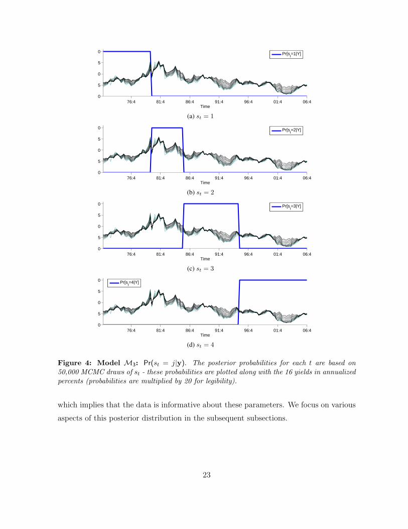
Our first set of findings relate to the timing of the change-points. Information about
the change-points is gleaned from the sampled sequence of the states. Further details
about how this is done can be obtained from Chib (1998). Of particular interest are
the posterior probabilities of the timing of the regime changes. These probabilities are
given in Figure 4. The figure reveals that the first 32 quarters (the first 8 years) belong
to the first regime, the next 23 quarters (about 6 years) to the second, the next 38
quarters (about 9.5 years) to the third, and the remaining quarters to the fourth regime.
Rudebusch and Wu (2007) also find a change point in the year of 1985. The finding of a
break point in 1995 is striking as it has not been isolated from previous regime-change
models.
We would like to emphasize that our estimates of the change points from the models
without macro factors are exactly the same as those from the change point models with
macro factors. We do not report those results in the interest of space. In addition, the
results are not sensitive to our choice of 16 maturities, as we have confirmed.
4.3 Parameter Estimates
Table 3 summarizes the posterior distribution of the parameters. One point to note is
that the posterior densities are generally different from the prior given in section 3.2,
22
76:4 81:4 86:4 91:4 96:4 01:4 06:40
5
10
15
20
Time
Pr[st=1|Y]
(a) st = 1
76:4 81:4 86:4 91:4 96:4 01:4 06:40
5
10
15
20
Time
Pr[st=2|Y]
(b) st = 2
76:4 81:4 86:4 91:4 96:4 01:4 06:40
5
10
15
20
Time
Pr[st=3|Y]
(c) st = 3
76:4 81:4 86:4 91:4 96:4 01:4 06:40
5
10
15
20
Time
Pr[st=4|Y]
(d) st = 4
Figure 4: Model M3: Pr(st = j|y). The posterior probabilities for each t are based on50,000 MCMC draws of st - these probabilities are plotted along with the 16 yields in annualizedpercents (probabilities are multiplied by 20 for legibility).
which implies that the data is informative about these parameters. We focus on various
aspects of this posterior distribution in the subsequent subsections.
23

Regime 1 Regime 2 Regime 3 Regime 4
0.90 0.07 0.15 0.95 -0.01 0.03 0.92 0.15 0.31 0.93 0.04 0.23(0.06) (0.10) (0.15) (0.03) (0.07) (0.06) (0.06) (0.21) (0.17) (0.04) (0.17) (0.29)
G -0.24 0.67 -0.07 -0.07 0.73 -0.10 0.15 0.35 0.08 0.02 0.91 0.01(0.26) (0.23) (0.12) (0.05) (0.05) (0.03) (0.06) (0.14) (0.08) (0.02) (0.13) (0.06)-0.06 -0.16 0.26 0.09 -0.35 0.52 -0.04 0.00 0.34 -0.03 -0.37 0.19(0.25) (0.23) (0.17) (0.17) (0.24) (0.17) (0.09) (0.21) (0.13) (0.08) (0.26) (0.15)
µ 0.00 4.99 3.54 0.00 5.88 2.63 0.00 2.56 2.62 0.00 1.49 3.22×400 (2.17) (0.90) (0.41) (1.00) (0.41) (0.49) (0.80) (0.53)
1.00 1.00 1.00 1.00
L 0.11 1.72 0.10 1.48 0.11 0.74 -0.47 0.82×400 (0.40) (0.19) (0.44) (0.13) (0.34) (0.13) (0.59) (0.12)
-0.67 -0.62 4.28 0.24 0.27 4.58 -0.55 -0.18 2.00 -0.13 -0.20 2.03(0.88) (0.39) (0.14) (0.62) (0.41) (0.17) (0.56) (0.14) (0.12) (0.89) (0.14) (0.11)
δ1 9.23 2.78 4.42 4.34×400 (1.69) (1.60) (1.18) (1.00)
δ2 1.16 0.09 0.17 1.29 0.25 0.16 0.72 0.31 0.26 0.57 0.56 0.10(0.13) (0.23) (0.22) (0.16) (0.23) (0.15) (0.09) (0.26) (0.21) (0.07) (0.37) (0.25)
γ -0.28 -0.40 -0.22 -0.34 -0.65 -0.21 -0.58 -0.56 -0.05 -0.34 -0.25 -0.19(0.28) (0.30) (0.26) (0.25) (0.21) (0.26) (0.28) (0.33) (0.24) (0.25) (0.25) (0.27)
Φ 0.99 0.98 0.93 0.53 0.89 0.65 0.91 0.94 0.98 0.98 0.93 0.98(1.08) (1.09) (1.08) (1.07) (1.08) (1.12) (1.08) (1.09) (1.09) (1.09) (1.10) (1.09)
p00 0.934(0.028)
p11 0.986(0.004)
p22 0.987(0.003)
Table 3: Model M3: Parameter estimates. This table presents the posterior meanand standard deviation based on 50,000 MCMC draws beyond a burn-in of 5,000. The 95%credibility interval of parameters in bold face does not contain 0. Standard deviations are inparenthesis. The yields are of 1, 2, 3, 4, 5, 6, 7, 8, 10, 12, 16, 20, 24, 28, 36 and 40 quartersmaturity bonds. Values without standard deviations are fixed by the identification restrictions.
4.3.1 Factor Process
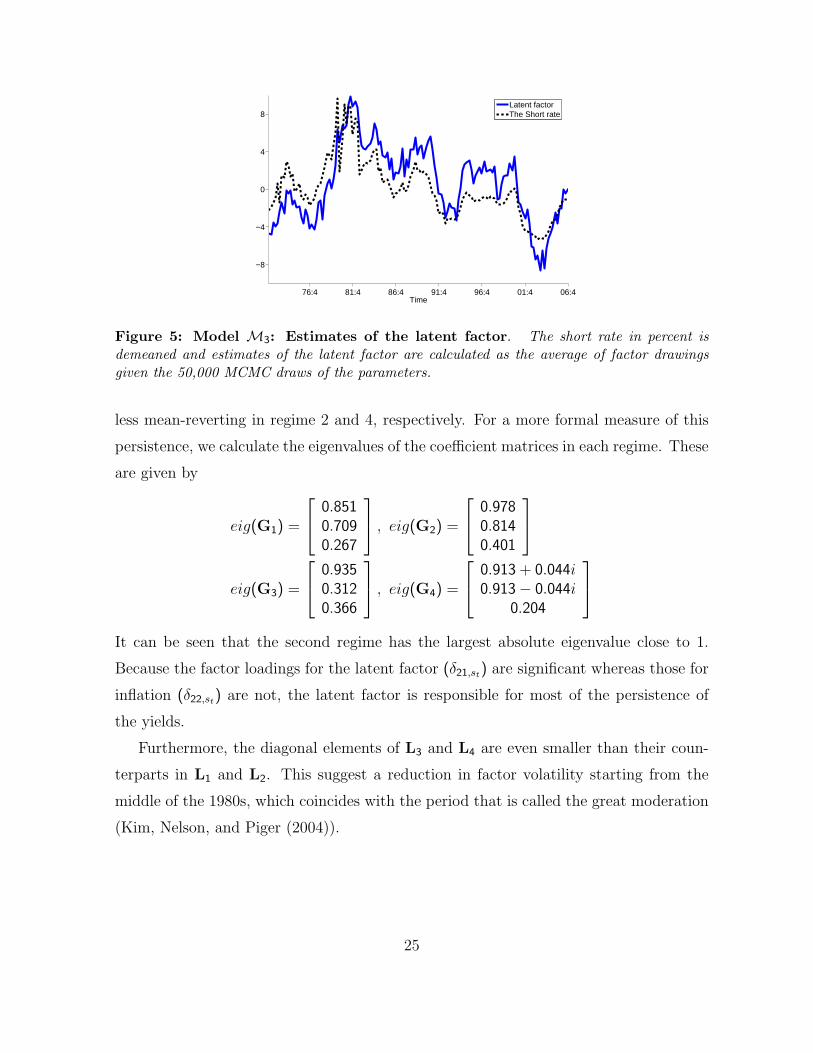
Figure 5 plots the average dynamics of the latent factors along with the short rate.
This figure demonstrates that the latent factor movements are very close to those of the
short rate. The estimates of the matrix G for each regime show that the mean-reversion
coefficient matrix is almost diagonal. The latent factor and inflation rate also display
different degrees of persistence across regimes. In particular, the relative magnitudes
of the diagonal elements indicates that the latent factor and the inflation factor are
24
76:4 81:4 86:4 91:4 96:4 01:4 06:4
−8
−4
0
4
8
Time
Latent factorThe Short rate
Figure 5: Model M3: Estimates of the latent factor. The short rate in percent isdemeaned and estimates of the latent factor are calculated as the average of factor drawingsgiven the 50,000 MCMC draws of the parameters.
less mean-reverting in regime 2 and 4, respectively. For a more formal measure of this
persistence, we calculate the eigenvalues of the coefficient matrices in each regime. These
are given by
eig(G1) =
0.8510.7090.267
, eig(G2) =
0.9780.8140.401
eig(G3) =
0.9350.3120.366
, eig(G4) =
0.913 + 0.044i0.913− 0.044i
0.204
It can be seen that the second regime has the largest absolute eigenvalue close to 1.
Because the factor loadings for the latent factor (δ21,st) are significant whereas those for
inflation (δ22,st) are not, the latent factor is responsible for most of the persistence of
the yields.
Furthermore, the diagonal elements of L3 and L4 are even smaller than their coun-
terparts in L1 and L2. This suggest a reduction in factor volatility starting from the
middle of the 1980s, which coincides with the period that is called the great moderation
(Kim, Nelson, and Piger (2004)).
25
4.3.2 Factor Loadings
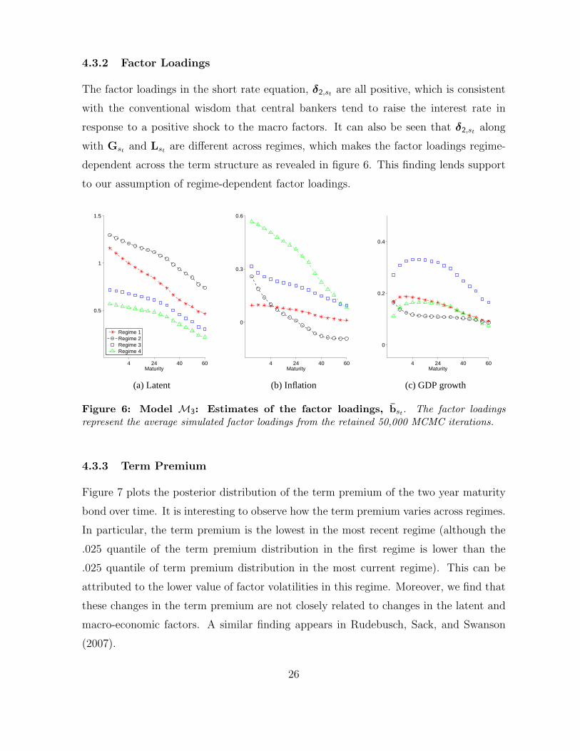
The factor loadings in the short rate equation, δ2,st are all positive, which is consistent
with the conventional wisdom that central bankers tend to raise the interest rate in
response to a positive shock to the macro factors. It can also be seen that δ2,st along
with Gst and Lst are different across regimes, which makes the factor loadings regime-
dependent across the term structure as revealed in figure 6. This finding lends support
to our assumption of regime-dependent factor loadings.
4 24 40 60
0.5
1
1.5
Maturity
Regime 1Regime 2Regime 3Regime 4
4 24 40 60
0
0.3
0.6
Maturity4 24 40 60
0
0.2
0.4
Maturity
(a) Latent (b) Inflation (c) GDP growth
Figure 6: Model M3: Estimates of the factor loadings, bst . The factor loadingsrepresent the average simulated factor loadings from the retained 50,000 MCMC iterations.
4.3.3 Term Premium
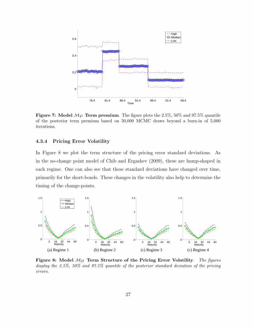
Figure 7 plots the posterior distribution of the term premium of the two year maturity
bond over time. It is interesting to observe how the term premium varies across regimes.
In particular, the term premium is the lowest in the most recent regime (although the
.025 quantile of the term premium distribution in the first regime is lower than the
.025 quantile of term premium distribution in the most current regime). This can be
attributed to the lower value of factor volatilities in this regime. Moreover, we find that
these changes in the term premium are not closely related to changes in the latent and
macro-economic factors. A similar finding appears in Rudebusch, Sack, and Swanson
(2007).
26
76:4 81:4 86:4 91:4 96:4 01:4 06:4
0
0.2
0.4
0.6
Time
HighMedianLow
Figure 7: ModelM3: Term premium. The figure plots the 2.5%, 50% and 97.5% quantileof the posterior term premium based on 50,000 MCMC draws beyond a burn-in of 5,000iterations.
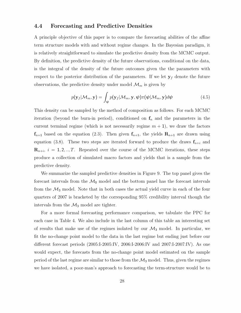
4.3.4 Pricing Error Volatility
In Figure 8 we plot the term structure of the pricing error standard deviations. As
in the no-change point model of Chib and Ergashev (2009), these are hump-shaped in
each regime. One can also see that these standard deviations have changed over time,
primarily for the short-bonds. These changes in the volatility also help to determine the
timing of the change-points.
3 16 32 44 600
0.5
1
1.5
Maturity
HighMedianLow
3 16 32 44 600
0.5
1
1.5
Maturity3 16 32 44 60
0
0.5
1
1.5
Maturity3 16 32 44 60
0
0.5
1
1.5
Maturity
(a) Regime 1 (b) Regime 2 (c) Regime 3 (c) Regime 4
Figure 8: Model M3: Term Structure of the Pricing Error Volatility. The figuresdisplay the 2.5%, 50% and 97.5% quantile of the posterior standard deviation of the pricingerrors.
27
4.4 Forecasting and Predictive Densities
A principle objective of this paper is to compare the forecasting abilities of the affine
term structure models with and without regime changes. In the Bayesian paradigm, it
is relatively straightforward to simulate the predictive density from the MCMC output.
By definition, the predictive density of the future observations, conditional on the data,
is the integral of the density of the future outcomes given the the parameters with
respect to the posterior distribution of the parameters. If we let yf denote the future
observations, the predictive density under model Mm is given by
p(yf |Mm,y) =
∫ψ
p(yf |Mm,y,ψ)π(ψ|Mm,y)dψ (4.5)
This density can be sampled by the method of composition as follows. For each MCMC
iteration (beyond the burn-in period), conditioned on fn and the parameters in the
current terminal regime (which is not necessarily regime m + 1), we draw the factors
fn+1 based on the equation (2.3). Then given fn+1, the yields Rn+1 are drawn using
equation (3.8). These two steps are iterated forward to produce the draws fn+i and
Rn+i, i = 1, 2, .., T . Repeated over the course of the MCMC iterations, these steps
produce a collection of simulated macro factors and yields that is a sample from the
predictive density.
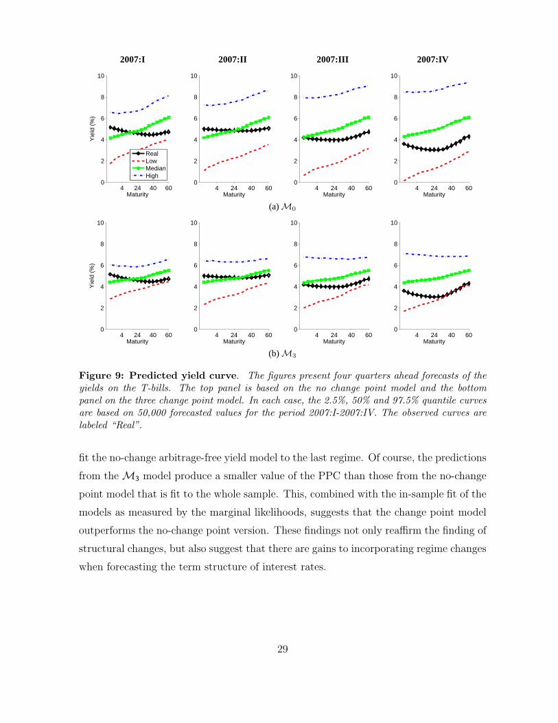
We summarize the sampled predictive densities in Figure 9. The top panel gives the
forecast intervals from the M0 model and the bottom panel has the forecast intervals
from the M3 model. Note that in both cases the actual yield curve in each of the four
quarters of 2007 is bracketed by the corresponding 95% credibility interval though the
intervals from the M3 model are tighter.
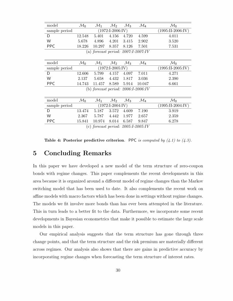
For a more formal forecasting performance comparison, we tabulate the PPC for
each case in Table 4. We also include in the last column of this table an interesting set
of results that make use of the regimes isolated by our M3 model. In particular, we
fit the no-change point model to the data in the last regime but ending just before our
different forecast periods (2005:I-2005:IV, 2006:I-2006:IV and 2007:I-2007:IV). As one
would expect, the forecasts from the no-change point model estimated on the sample
period of the last regime are similar to those from theM3 model. Thus, given the regimes
we have isolated, a poor-man’s approach to forecasting the term-structure would be to
28
2007:I 2007:II 2007:III 2007:IV
4 24 40 600
2
4
6
8
10
Maturity
Yie
ld (
%)
RealLowMedianHigh
4 24 40 600
2
4
6
8
10
Maturity4 24 40 60
0
2
4
6
8
10
Maturity4 24 40 60
0
2
4
6
8
10
Maturity
(a)M0
4 24 40 600
2
4
6
8
10
Maturity
Yie
ld (
%)
4 24 40 600
2
4
6
8
10
Maturity4 24 40 60
0
2
4
6
8
10
Maturity4 24 40 60
0
2
4
6
8
10
Maturity
(b)M3
Figure 9: Predicted yield curve. The figures present four quarters ahead forecasts of theyields on the T-bills. The top panel is based on the no change point model and the bottompanel on the three change point model. In each case, the 2.5%, 50% and 97.5% quantile curvesare based on 50,000 forecasted values for the period 2007:I-2007:IV. The observed curves arelabeled “Real”.
fit the no-change arbitrage-free yield model to the last regime. Of course, the predictions
from theM3 model produce a smaller value of the PPC than those from the no-change
point model that is fit to the whole sample. This, combined with the in-sample fit of the
models as measured by the marginal likelihoods, suggests that the change point model
outperforms the no-change point version. These findings not only reaffirm the finding of
structural changes, but also suggest that there are gains to incorporating regime changes
when forecasting the term structure of interest rates.
29
model M0 M1 M2 M3 M4 M0
sample period (1972:I-2006:IV) (1995:II-2006:IV)D 12.548 5.401 4.156 4.720 4.599 4.011W 5.678 4.896 4.201 3.415 2.902 3.520PPC 18.226 10.297 8.357 8.126 7.501 7.531
(a) forecast period: 2007:I-2007:IV
model M0 M1 M2 M3 M4 M0
sample period (1972:I-2005:IV) (1995:II-2005:IV)D 12.606 5.799 4.157 4.097 7.011 4.271W 2.137 5.658 4.432 1.817 3.036 2.390PPC 14.743 11.457 8.589 5.914 10.047 6.661
(b) forecast period: 2006:I-2006:IV
model M0 M1 M2 M3 M4 M0
sample period (1972:I-2004:IV) (1995:II-2004:IV)D 13.474 5.187 3.572 4.609 7.190 3.919W 2.367 5.787 4.442 1.977 2.657 2.359PPC 15.841 10.974 8.014 6.587 9.847 6.278
(c) forecast period: 2005:I-2005:IV
Table 4: Posterior predictive criterion. PPC is computed by (4.1) to (4.3).
5 Concluding Remarks
In this paper we have developed a new model of the term structure of zero-coupon
bonds with regime changes. This paper complements the recent developments in this
area because it is organized around a different model of regime changes than the Markov
switching model that has been used to date. It also complements the recent work on
affine models with macro factors which has been done in settings without regime changes.
The models we fit involve more bonds than has ever been attempted in the literature.
This in turn leads to a better fit to the data. Furthermore, we incorporate some recent
developments in Bayesian econometrics that make it possible to estimate the large scale
models in this paper.
Our empirical analysis suggests that the term structure has gone through three
change points, and that the term structure and the risk premium are materially different
across regimes. Our analysis also shows that there are gains in predictive accuracy by
incorporating regime changes when forecasting the term structure of interest rates.
30
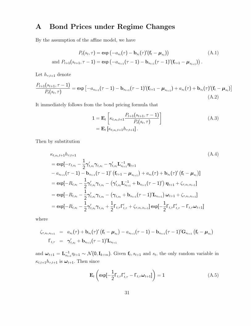
A Bond Prices under Regime Changes
By the assumption of the affine model, we have
Pt(st, τ) = exp(−ast(τ)− bst(τ)′(ft − µst
))
(A.1)
and Pt+1(st+1, τ − 1) = exp(−ast+1(τ − 1)− bst+1(τ − 1)′(ft+1 − µst+1
)).
Let hτ,t+1 denote
Pt+1(st+1, τ − 1)
Pt(st, τ)= exp
[−ast+1(τ − 1)− bst+1(τ − 1)′(ft+1 − µst+1
) + ast(τ) + bst(τ)′(ft − µst)]
(A.2)
It immediately follows from the bond pricing formula that
1 = Et
[κt,st,t+1
Pt+1(st+1, τ − 1)
Pt(st, τ)
](A.3)
= Et [κt,st,t+1hτ,t+1] .
Then by substitution
κt,st,t+1hτ,t+1 (A.4)
= exp[−rt,st −1
2γ ′t,st
γt,st− γ ′t,st
L−1st+1ηt+1
− ast+1(τ − 1)− bst+1(τ − 1)′(ft+1 − µst+1
)+ ast(τ) + bst(τ)′
(ft − µst
)]
= exp[−Rt,st −1
2γ ′t,st
γt,st−(γ ′t,st
L−1st+1
+ bst+1(τ − 1)′)ηt+1 + ζτ,st,st+1]
= exp[−Rt,st −1
2γ ′t,st
γt,st−(γt,st
+ bst+1(τ − 1)′Lst+1
)ωt+1 + ζτ,st,st+1]
= exp[−Rt,st −1
2γ ′t,st
γt,st+
1
2Γt,τΓ′t,τ + ζτ,st,st+1] exp[−1
2Γt,τΓ′t,τ − Γt,τωt+1]
where
ζτ,st,st+1 = ast(τ) + bst(τ)′(ft − µst
)− ast+1(τ − 1)− bst+1(τ − 1)′Gst+1
(ft − µst
)Γt,τ = γ ′t,st
+ bst+1(τ − 1)′Lst+1
and ωt+1 = L−1st+1
ηt+1 ∼ N (0, Ik+m). Given ft, st+1 and st, the only random variable in
κt,t+1hτ,t+1 is ωt+1. Then since
Et
(exp[−1
2Γt,τΓ′t,τ − Γt,τωt+1]
)= 1 (A.5)
31
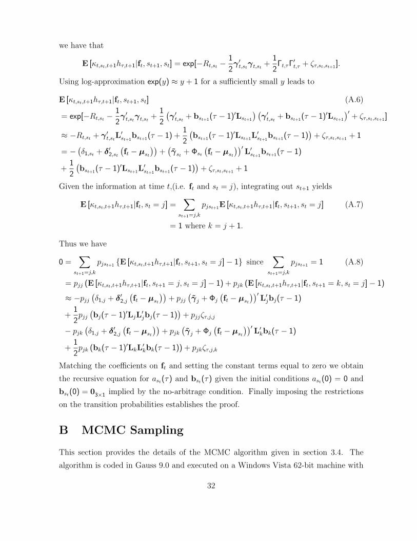
we have that
E [κt,st,t+1hτ,t+1|ft, st+1, st] = exp[−Rt,st −1
2γ ′t,st
γt,st+
1
2Γt,τΓ′t,τ + ζτ,st,st+1].
Using log-approximation exp(y) ≈ y + 1 for a sufficiently small y leads to
E [κt,st,t+1hτ,t+1|ft, st+1, st] (A.6)
= exp[−Rt,st −1
2γ ′t,st
γt,st+
1
2
(γ ′t,st
+ bst+1(τ − 1)′Lst+1
) (γ ′t,st
+ bst+1(τ − 1)′Lst+1
)′+ ζτ,st,st+1]
≈ −Rt,st + γ ′t,stL′st+1
bst+1(τ − 1) +1
2
(bst+1(τ − 1)′Lst+1L
′st+1
bst+1(τ − 1))
+ ζτ,st,st+1 + 1
= −(δ1,st + δ′2,st
(ft − µst
))+(γst
+ Φst
(ft − µst
))′L′st+1
bst+1(τ − 1)
+1
2
(bst+1(τ − 1)′Lst+1L
′st+1
bst+1(τ − 1))
+ ζτ,st,st+1 + 1
Given the information at time t,(i.e. ft and st = j), integrating out st+1 yields
E [κt,st,t+1hτ,t+1|ft, st = j] =∑
st+1=j,k
pjst+1E [κt,st,t+1hτ,t+1|ft, st+1, st = j] (A.7)
= 1 where k = j + 1.
Thus we have
0 =∑
st+1=j,k
pjst+1 E [κt,st,t+1hτ,t+1|ft, st+1, st = j]− 1 since∑
st+1=j,k
pjst+1 = 1 (A.8)
= pjj (E [κt,st,t+1hτ,t+1|ft, st+1 = j, st = j]− 1) + pjk (E [κt,st,t+1hτ,t+1|ft, st+1 = k, st = j]− 1)
≈ −pjj(δ1,j + δ′2,j
(ft − µst
))+ pjj
(γj + Φj
(ft − µst
))′L′jbj(τ − 1)
+1
2pjj(bj(τ − 1)′LjL
′jbj(τ − 1)
)+ pjjζτ,j,j
− pjk(δ1,j + δ′2,j
(ft − µst
))+ pjk
(γj + Φj
(ft − µst
))′L′kbk(τ − 1)
+1
2pjk (bk(τ − 1)′LkL
′kbk(τ − 1)) + pjkζτ,j,k
Matching the coefficients on ft and setting the constant terms equal to zero we obtain
the recursive equation for ast(τ) and bst(τ) given the initial conditions ast(0) = 0 and
bst(0) = 03×1 implied by the no-arbitrage condition. Finally imposing the restrictions
on the transition probabilities establishes the proof.
B MCMC Sampling
This section provides the details of the MCMC algorithm given in section 3.4. The
algorithm is coded in Gauss 9.0 and executed on a Windows Vista 62-bit machine with
32
a 2.66 GHz Intel Quad Core2 CPU. About 12 days are needed to generate 50,000 MCMC
draws in the 3 change-point model. In contrast, a random-walk M-H algorithm takes
about 2 days to complete 1 million iterations but with unknown reliability and much
less efficient exploration (Chib and Ramamurthy (2009)).
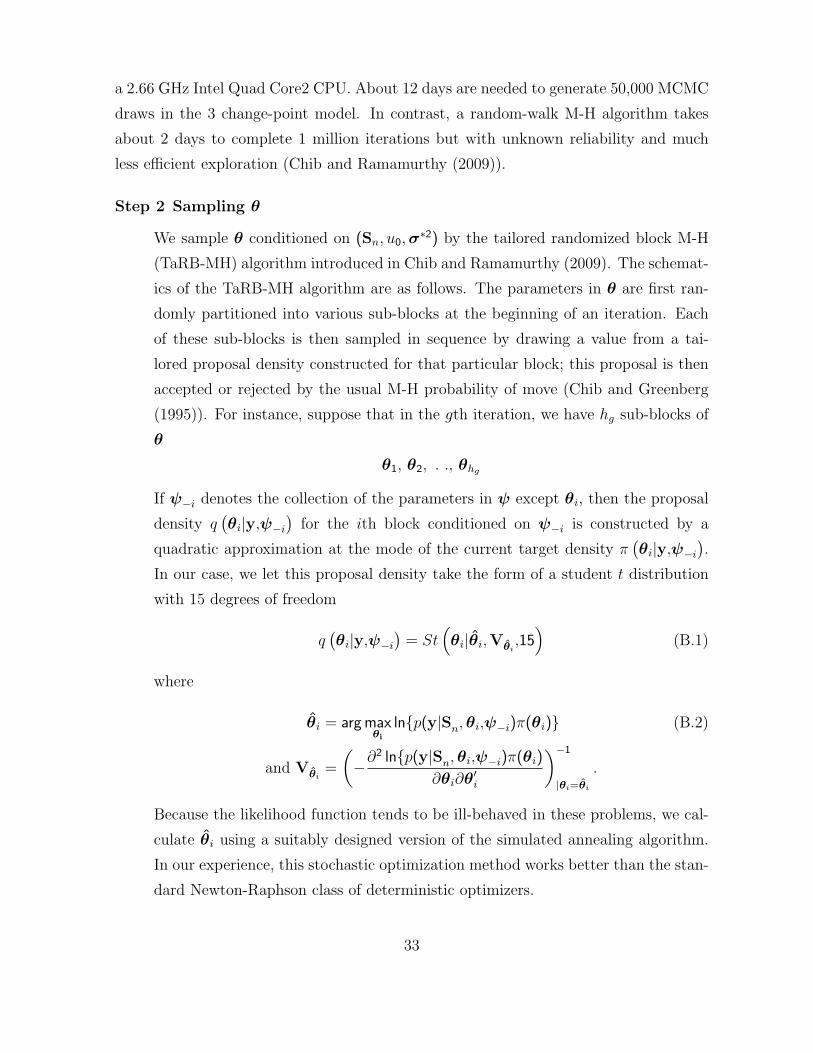
Step 2 Sampling θ
We sample θ conditioned on (Sn, u0,σ∗2) by the tailored randomized block M-H
(TaRB-MH) algorithm introduced in Chib and Ramamurthy (2009). The schemat-
ics of the TaRB-MH algorithm are as follows. The parameters in θ are first ran-
domly partitioned into various sub-blocks at the beginning of an iteration. Each
of these sub-blocks is then sampled in sequence by drawing a value from a tai-
lored proposal density constructed for that particular block; this proposal is then
accepted or rejected by the usual M-H probability of move (Chib and Greenberg
(1995)). For instance, suppose that in the gth iteration, we have hg sub-blocks of
θ
θ1, θ2, . ., θhg
If ψ−i denotes the collection of the parameters in ψ except θi, then the proposal
density q(θi|y,ψ−i
)for the ith block conditioned on ψ−i is constructed by a
quadratic approximation at the mode of the current target density π(θi|y,ψ−i
).
In our case, we let this proposal density take the form of a student t distribution
with 15 degrees of freedom
q(θi|y,ψ−i
)= St
(θi|θi,Vθi
,15)
(B.1)
where
θi = arg maxθi
lnp(y|Sn,θi,ψ−i)π(θi) (B.2)
and Vθi=
(−∂
2 lnp(y|Sn,θi,ψ−i)π(θi)
∂θi∂θ′i
)−1
|θi=θi
.
Because the likelihood function tends to be ill-behaved in these problems, we cal-
culate θi using a suitably designed version of the simulated annealing algorithm.
In our experience, this stochastic optimization method works better than the stan-
dard Newton-Raphson class of deterministic optimizers.
33

We then generate a proposal value θ†i which, upon satisfying all the constraints, is
accepted as the next value in the chain with probability
α(θ(g−1)i ,θ†i |y,ψ−i) (B.3)
= min
p(y|Sn,θ†i ,ψ−i)π(θ†i )
p(y|Sn,θ(g−1)i ,ψ−i)π(θ
(g−1)i )
St(θ(g−1)i |θi,Vθi
,15)
St(θ†j|θi,Vθi,15)
, 1
.
If θ†i violates any of the constraints inR, it is immediately rejected. The simulation
of θ is complete when all the sub-blocks
π(θ1|y,Sn,ψ−1
), π(θ2|y,Sn,ψ−2
), . . . , π(θhg |y,Sn,ψ−hg
) (B.4)
are sequentially updated as above.
Step 3 Sampling the initial factor
Given the prior in equation (3.14), u0 is updated conditioned on θ,m0 and f1 = (u1
m′1)′, where m0 is given by data and u1 is obtained from the equation (3.5). In
the following, it is assumed that all the underlying coefficients are those in regime
0. Then
u0|f1,θ∼N1 (u0,U0) (B.5)
where
u0 = U0
(Σ−1u +H∗′Ω∗11,0u
∗1
), U0 =
(Σ−1u +H∗′Ω∗11,1H
∗)and on letting
G0 =
(G11,1 G12,1
G21,1 G22,1
), Ω1 =
(Ω11,1 Ω12,1
Ω21,1 Ω22,1
)H∗ = G11,1−Ω12,1Ω−1
22,1G21,1, Ω∗11,1 = Ω11,1−Ω12,1Ω−122,1Ω21,1
u∗1 = u1 − Ω12,1Ω−122,1(m1 − µm,1) +
(Ω12,1Ω−1
22,1G22,1−G12,1
)(m0 − µm,1)
Step 4 Sampling regimes
In this step one samples the states from p[Sn|In,ψ] where In is the history of the
outcomes up to time n. This is done according to the method of Chib (1996) and
Chib (1998) by sampling Sn in a single block from the output of one forward and
backward pass through the data.
34
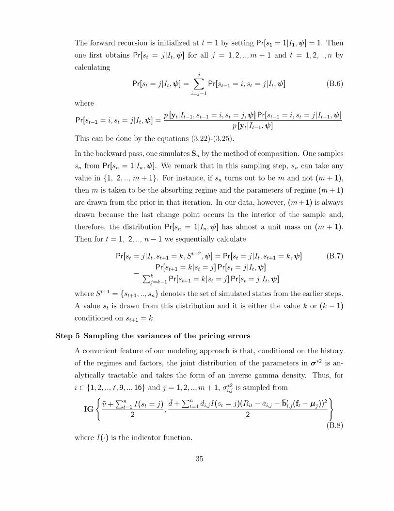
The forward recursion is initialized at t = 1 by setting Pr[s1 = 1|I1,ψ] = 1. Then
one first obtains Pr[st = j|It,ψ] for all j = 1, 2, ..,m + 1 and t = 1, 2, .., n by
calculating
Pr[st = j|It,ψ] =
j∑i=j−1
Pr[st−1 = i, st = j|It,ψ] (B.6)
where
Pr[st−1 = i, st = j|It,ψ] =p [yt|It−1, st−1 = i, st = j,ψ] Pr[st−1 = i, st = j|It−1,ψ]
p [yt|It−1,ψ]
This can be done by the equations (3.22)-(3.25).
In the backward pass, one simulates Sn by the method of composition. One samples
sn from Pr[sn = 1|In,ψ]. We remark that in this sampling step, sn can take any
value in 1, 2, .., m + 1. For instance, if sn turns out to be m and not (m + 1),
then m is taken to be the absorbing regime and the parameters of regime (m+ 1)
are drawn from the prior in that iteration. In our data, however, (m+ 1) is always
drawn because the last change point occurs in the interior of the sample and,
therefore, the distribution Pr[sn = 1|In,ψ] has almost a unit mass on (m + 1).
Then for t = 1, 2, .., n− 1 we sequentially calculate
Pr[st = j|It, st+1 = k, St+2,ψ] = Pr[st = j|It, st+1 = k,ψ] (B.7)
=Pr[st+1 = k|st = j] Pr[st = j|It,ψ]∑k
j=k−1 Pr[st+1 = k|st = j] Pr[st = j|It,ψ]
where St+1 = st+1, .., sn denotes the set of simulated states from the earlier steps.
A value st is drawn from this distribution and it is either the value k or (k − 1)
conditioned on st+1 = k.
Step 5 Sampling the variances of the pricing errors
A convenient feature of our modeling approach is that, conditional on the history
of the regimes and factors, the joint distribution of the parameters in σ∗2 is an-
alytically tractable and takes the form of an inverse gamma density. Thus, for
i ∈ 1, 2, .., 7, 9, .., 16 and j = 1, 2, ..,m + 1, σ∗2i,j is sampled from
IG
v +
∑nt=1 I (st = j)
2,d +
∑nt=1 di,jI (st = j)(Rit − ai,j − b′i,j(ft − µj))2
2
(B.8)
where I (·) is the indicator function.
35
References
Ang, A., Bekaert, G., and Wei, M. (2008), “The term structure of real rates and expected
inflation,” Journal of Finance, 63, 797–849.
Ang, A., Dong, S., and Piazzesi, M. (2007), “No-arbitrage Taylor rules,” Columbia
University working paper.
Ang, A. and Piazzesi, M. (2003), “A no-arbitrage vector autoregression of term structure
dynamics with macroeconomic and latent variables,” Journal of Monetary Economics,
50, 745–787.
Bansal, R. and Zhou, H. (2002), “Term structure of interest rates with regime shifts,”
Journal of Finance, LVII, 463–473.
Chen, R. and Scott, L. (2003), “ML estimation for a multifactor equilibrium model of
the term structure,” Journal of Fixed Income, 27, 14–31.
Chib, S. (1995), “Marginal likelihood from the Gibbs output,” Journal of the American
Statistical Association, 90, 1313–1321.
— (1996), “Calculating posterior distributions and modal estimates in Markov mixture
models,” Journal of Econometrics, 75, 79–97.
— (1998), “Estimation and comparison of multiple change-point models,” Journal of
Econometrics, 86, 221–241.
— (2001), “Markov chain Monte Carlo methods: computation and inference,” in Hand-
book of Econometrics, eds. Heckman, J. and Leamer, E., North Holland, Amsterdam,
vol. 5, pp. 3569–3649.
Chib, S. and Ergashev, B. (2009), “Analysis of multi-factor affine yield curve models,”
Journal of the American Statistical Association, forthcoming.
Chib, S. and Greenberg, E. (1995), “Understanding the Metropolis-Hastings algorithm,”
American Statistician, 49, 327–335.
36

Chib, S. and Jeliazkov, I. (2001), “Marginal likelihood from the Metropolis-Hastings
output,” Journal of the American Statistical Association, 96, 270–281.
Chib, S. and Ramamurthy, S. (2009), “Tailored randomized block MCMC methods with
application to DSGE models,” Journal of Econometrics, forthcoming.
Dai, Q. and Singleton, K. J. (2000), “Specification analysis of affine term structure
models,” Journal of Finance, 55, 1943–1978.
Dai, Q., Singleton, K. J., and Yang, W. (2007), “Regime shifts in a dynamic term
structure model of U.S. treasury bond yields,” Review of Financial Studies, 20, 1669–
1706.
Duffie, G. and Kan, R. (1996), “A yield-factor model of interest rates,” Mathematical
Finance, 6, 379–406.
Gelfand, A. E. and Ghosh, S. K. (1998), “Model choice: A minimum posterior predictive
loss approach,” Biometrika, 85, 1–11.
Gurkaynak, R. S., Sack, B., and Wright, J. H. (2007), “The U.S. treasury yield curve:
1961 to the present,” Journal of Monetary Economics, 54, 2291–2304.
Kim, C. J., Nelson, C. R., and Piger, J. (2004), “The less volatile U.S. economy: a
Bayesian investigation of timing, breadth, and potential explanations,” Journal of
Business and Economic Statistics, 22, 80–93.
Rudebusch, G. D., Sack, B. P., and Swanson, E. T. (2007), “Macroeconomic implications
of changes in the term premium,” Federal Reserve Bank of St Louis Review, 89, 241–
269.
Rudebusch, G. D. and Wu, T. (2007), “Accounting for a shift in term structure behavior
with no-arbitrage and macro-finance models,” Journal of Money, Credit and Banking,
39, 395–422.
37