Internal Documents

INDUSTRY AND ENERGY DEPARTMENT WORKING PAENERGY SERIES PAPER No. 52

Electricity Pricing:Conventional Views and New Concepts

March 1992

ji,(r, .- 4 . .. . . .~~~ .- 0 .

The World Bank Industry and Energy Department, PRE

s SE g -o °ILE.COPY

Pub

lic D

iscl

osur

e A

utho

rized

Pub

lic D

iscl

osur

e A

utho

rized

Pub

lic D

iscl

osur

e A

utho

rized

Pub

lic D

iscl

osur

e A

utho

rized

ELECTRICITY PRICING: CONVENTIONAL VIEWS AND NEW CONCEPTS

by

Witold Teplitz-Sembitzky

Energy Development DivisionIndustry and Energy Department

Sector and Operations Policy

March 1992

Copyright (c) 1992The World Bank1818 H Street, N.W.Washington, D.C. 20433U.S.A.

T. s report is one of a series issued by the Industry and Energy Departnent for theinformation and guidance of Bank staff. The report may not be published or quoted asrepresenting the views of the Bank Group, nor does the Bank Group accept responsibilityfor its accuracy or completeness.

The author is grateful to Mr. Amadou Cisse for valuable discussions, critique, andsuggestions. Helpful comments on an earlier draft of the paper were also provided byMr. John Besant-Jones.

Execufive Summary

Both in theory and practice, electricity pricing is a difficult and complex subject. This paperfocuses on the theoretical aspects of electricity pricing and thus neither resolves the manypractical problems of designing electricity tariffs nor offers an agenda for immediate action.Instead, it attempts to clarify the debate over conventional and new theories of electricitypricing by examining the rationales of some basic assumptions about pricing, includingmarginal cost (MC) pricing, Ramsey-pricing, sustainable pricing, axiomatic pricing, averagecost pricing, priority service pricing, and price capping. The analysis suggests thatdoctrinaire adherence to marginal cost and efficiency principles may be inappropriate andinsufficiendy responsive to the uneveiu, rapidly changing, and often financially shaky powersectors of developing countries.

Electricity pricing is fraught with a number of complications that reflectessential technical characteristics of the power sector. To simplify matters, this paperdisregards spatial aspects of power transmission and distribution (i.e., restricts its focus tothe generation end). This still leaves the analysis to cope with key features that distinguishe!ectricity pricing from putting a price tag on, say, office supplies:

1. Electricity is nonstorable; it is generated at different times to serve loads of differentsize at different priority levels. Thus, power generation is a multiproduct industry inwhich the outputs can be indexed by time of use and priority of service.

2. Power generation is an exarnple of joint production that exhibits economies of scopefrom horizontal integration and, thus, is cheaper than separate production. Putanother way, generating capacity qualifies as a public input (i.e., an input that canproduce several outputs or loads on a nonrival and nonexcludable basis).

3. Economies of scope entail multiproduct economies of scale (i.e., total costs exceedthe weighted average of marginal costs defined along a ray from the origin). By thesame token, the incremental costs of generating a particular load fall short of thecorresponding stand-alone generation costs. In addition, there may existproduct/load-specific scale economies.

4. Power sector investments are to a significant extent transaction-specific and,therefore, sunk (i.e., the worth of the sector's assets cannot be recovered entirelyupon exit.

These features have several implications:

1. Allocating costs and setting prices across different outputs becomes a complex taskthat eludes single-product reasoning.

2. In the presence of sunk costs, the mechanics of competition cannot be expected toimnplicitly .egulate or discipline the sector in an efficient and reliable manner. Someform of explicit regulation will be needed to ensure that sector performance ingeneral and tariff setting in particular live up to the standards ascribed to areasonably compeddve market.

3. Under economies of scope, the competitive ideal of independent, atomistic suppliersis at variance with the requirements of an efficient industry structure. At theminimum, efficiency calls for central coordination (merit order dispatch) of a limitednumber of suppliers. It may even warrant a structure based on a single supplier

- ii -

(natural monopoly). The latter case would apply if a monopoly enjoyed costadvantages with respect to any conceivable combination of outputs that the marketcan absorb.

The distinguishing features of the power sector notwithstanding, standardeconomic arguments suggest that in a multiproduct industry marginal costs (MC) are asvalid a benchmark for static efficiency pricing as in a single-product context. In fact,tailored to the characteristics of power generation, the ideal of multiproduct MC pricingassumes the form of time-of-use pricing, often referred to as peak-load pricing, or spotpricing, an upbeat variant of the MC principle that defines time in terms of instants.

The rationale for MC pricing is that it is necessary for an efficient allocationof resources that maximizes aggregate welfare. For that matter, efficient prices need to clearthe market and, as the notion of "spot pricing" emphasizes, should be based on short-runmarginal costs. Frequent disclaimers to the contrary, these requirements will not be met byprices based on long-run marginal cost (unless demand and supply are poised in a long-runeq"s'iium), let alone long-run average (incremental) costs. To make matters worse, inpractical applications the long-run approach to pricing of electricity usually is confined to ascalar measure of system costs that blurs the multiproduct nature of power generation.

MC pricing, however, is *n general not sufficient for economic efficiency. Itmay even be inefficient. For instance, if the electric -tility uses oublic funds that havepositive shadow costs, prices should exceed MC. Likewise, if MC pricing does not recovertotal costs, it may be better to charge financially viable prices iather than to balance theutility's accounts through indirect transfers.

Moreover, MC pricing can be rejected on equity grounds. Prices departingfrom MC may be justified as a substitute for imperfect taxation to redistribute income.Also, a switch to time-of-use pricing that improves on aggregate welfare but makes peak-load customers worse off may be considered unacceptable to the extent that it violates thePareto-principle.

Finally, the incentive framework may not be conducive to MC pricing, and aregulatory authority may not be in a position to successfully enforce MC prices. In fact, thelack of commitment on the part of the utility to charge efficient tariffs is pervasive in theabsence of disciplining market forces. Therefore, electric utility regulation is commonlydeemed a prerequisite for efficient pricing. Regulatory hierarchies, however, tend to beinefficient, too. In particular, utilities have an informational edge over the regulator and,thus, may evade agreed duties and covenants.

In short, although MC pricing is necessary for maximal welfare, real worldconditions rarely lend themselves to first-best solutions. If technical, institutional, oreconomic impediments spoil the decisionmakers' environment, a responsive pricing seategythat explicitly accounts for constraints is more likely to be efficient than is a doctrinaireadherence to the yardstick of marginal costs.

When MC pricing involves financial losses that the utility is required toavert, multiproduct Ramsey-pricing, which calls for markups over MC inverselyproportional to the elasticities of demand, ranks second from the viewpoint of economicefficiency. (In fact, it is first-rate with respect to the break-even constraint.) This is becauseit minimizes the partial equilibrium deadweight loss that financially viable prices departingfrom marginal costs tend to incur. Regrettably, however, the Ramsey rule-like the MCyardstick-only provides a necessary condition for second-best optimality. Whether or notRamsey pricing leads to a second-best outcome is an entirely different question. Applying

- iii -

the rule may be of no avail ir. the struggle for break-even constrained efficiency unlessdemand and supply are "well-behaved."

Another problem with Ramsey-pricing is that it may entail cross-subsidiesamong outputs and, thus, cross-subsidies among consumers. In this event, a utility acting asa second-best welfare maximizer is vulnerable to profitable, but inefficient entry (i.e., someconsumers have an incentive to defect to rival suppliers even though this would reduce thelevel of aggregate welfare). By the same token, Ramsey-pricing may be at odds withpolicies designed to instill competition in the power sector, because increased competitionreduces the scope for the large markups the Ramsey rule advocates in inelastic markets.

An alternative approach that counts on the merits ascribed to competitionwhile seeking to protect the incumbent udlity against inefficient entry has been suggested bythe "contestability" literature. The idea is that an efficient industry structure may besustainable with the aid of financially viable prices that keep customers satisfied and deterentry. By definition, sustainable prices must clear the market, recover costs, and rule outcross-subsidies. Unfortunately, such prices may be elusive that is, it may not be feasible tosafeguard an efficient industry structure with the help pricing policies alone. Apart fromthat, unsustainable Ramsey prices are welfare-superior to sustainable prices. Thus, one hasto trade off the virtues of sustainable prices against the potential welfare gains from strictRamsey-pricing.

Notwithstanding the doubts abo&. the feasibility and welfare properties ofsustainable pricing, the contestability literature h _ 4;Žawn attention to the crucial question ofwhe ther and to what extent a utility can be obliga ,- or impelled to put a particular pricingpolity into place. In this rega.d, the argument raised by the contestable market concept isthat the forces of potential entry bring prices on a path toward sustainability. Is there asimilar built-in mechanism that would induce a utility to adopt prices that are close toRamsey levels? The answer is no. Analogous to the case in which MC pricing is called forin the absence of reasonably competitive markets, there is no incentive mechanism thatwould prompt the utility to self-select Ramsey prices. Rather, Ramsey pricing, like MCpricing without competition, needs to be enforced through regulatory arrangements.Clearly, in practice, the disciplining forces behind sustainable prices may turn out to be asweak as is the incentive to implement Ramsey prices. The contestability literaturenevertheless made a strong point in highlighting the need to assess pricing rules in terms ofthe regulatory and incentive framework required for their implementation.

Interestingly enough, another line of argument, the axiomatic pricingapproach, does not focus on the contestability of markets, but reaches at a multiproduct costallocation procedure that may closely match the properties of sustainable prices. Theapproach hinges on the claim that prices, to be desirable, should satisfy a number ofconditions defined in terms of fairly plausible rules for cost accounting, including theprinciple of cost recovery. In the special case when costs are separable across outputs, theonly cost-based pricing mechanism that complies with this particular set of desiderata boilsdown to average cost (AC) pricing. In the context of power generation, this solution isequivalent to load-specific average cost pricing or time-of-use pricing, with the peak-loadprice based on average stand alone costs and off-peak prices set equal to the averageincremental costs of serving off-peak demand. Moreover, under economies of scope, load-specific average cost prices will be sustainable.

Apart from its affinity to the concept of sustainability, axiomatic pricing hasother appealing features. It "rationalizes" the debate over the desirability of pricing rules tothe extent that it can be derived as a conclusion from transparent premises. Its informationalrequirements are less demanding than are those of Ramsey-pricing. And if the

- lv -

decisionmaking process within the utility is decentralized along cost of profit centers, it isthe only mechanism that unambiguously rewards or penalizes good or bad performance.

On the other hand, axiomatic pricing has the disadvantage of forgoingpotential welfare gains that could be captured by discriminating across outputs/markets inthe style of Ramsey-pricing. And a weakness shared with MC, Ramsey-, and sustainablepricing is its lack of commitment. That is, there is no a priori reason why a utility should bekeen on axiomatic pricing (or AC-pricing) and at the same time pursue the goal of costminimization.

Ramsey-pricing, on the other hand, pinpoints a simple but pivotal pc' toolfor improvements on welfare that cost-based pricing strategies are unat ,o acco. .lish.By placing the focus on demand characteristics that may vary across markets -onsu- , o,both, the Ramsey approach increases the decisionmaker's degree of freedom in settir.,tariffs. Even though the inverse elasticity rule of Ramsey pricing is designed as a device forconstrained welfare-maximization, the logic underlying the approach can just as well beused to pursue the less zealous goal of making improvements in welfare feasible. In fact, inthe presence of consumers with diverse preferences, any uniform price charged per unit ofoutput and exceedir g marginal costs can be Pareto-dominated by an additional optionaltwo-part tariff, consisting of a fixed entry fee and a usage charge. This is because anincrease in the scope for choice, if properly designed, can make some consumers better offwithout making others, including the utility, worse off.

From a practical viewpoint, the main advantage of the optional pricingapproach to enhancing welfare is that it can be implemented without a comprehensiveknowledge of the consumers' demand functions. Clearly, the more information is availableto the decisionmaker, the better are the opportunities to fine-tune the options. In the extremecase, with perfect informnation, this strategy would result in the design of an optimalnonlinear tariff schedule that maximizes total welfare, subject to the utility's break-evenconstraint. By dint of discriminating continously across consumer classes in each market,such schedules Pareto-dominate linear Ramsey-pricing. Also, they will involve quantitydiscounts when (1) the elasticity of demand for an additional kWh (usage) increases withthe number of kWhs purchased, and (2) the excess willingness to pay for usage issufficiently large to justify the provision of additional capacity. Needless to say, theinformational requirements for achieving a constrained optimum with the help of nonlinearprices are even more forbidding than in the case of ordinary Ramsey-pricing. The principlemessage, though, remains valid: Flexibility, -that is, increasing the degree of freedom inpricing-is a means of improving both the consumers' well-being and the utility's accounts.

As it affects industry structure and sector performance, nonlinear pricing hasboth advantages and drawbacks. If the utility qualifies as a natural monopoly and ispermitted to charge nonlinear (discriminatory) tariffs, it may be able to foreclose entry andat the same time earn positive profits. Hence, it is conceivable that an inefficient utility willsurvive in contestable markets. By the same token, however, nonlinear pricing may help anotherwise unsustainable but efficient utility to withstand the threat of entry. This impliesthat even in the typical case in which the disciplining force of potential entry or intermodalcompetition is weak, nonlinear pricing may be ber,eficial rather than harmful or ruthless.

Priority service pricing is another example of how the mechL.aism of self-selection can improve on welfare and efficiency. Because outages at the generation end areunavoidable, even though the likelihood of their occurrence can be influenced through byproviding reserve capacity, the utility has to decide on reliability design targets and theallocation of shortfalls. By offering service contracts that charge a premium on electricity inlimited supply, the utility can encourage consumers to choose their preferred orders of

t ~~~~~~~~~~~~~~~~~~~- v -

priority in obtaining service. Moreover, by inducing consumers to reveal their willingnessto pay for "reliability," priority service pricing renders the separate calculation (estimatiop)of nutage costs-often tenuously derived-superfluous and thus eases tne task ofde m-rmining the optimal size of capacity. Again, because of informational and technical"0oA3-aints, optimal priority scrvice pricing will not be feasible hli practice. However, evenim,perfectly designed service conmacts are likely to improve welfare compared with theE .rnaave of random rationing.

In discerning and comparing the virtues of alternative pricing policies, oneshoulc not 1.,se sight of the fundamental dilemma mentioned before. In the power sectorthere is no "invisible hand," not even a workably efficient one. The analogy of a perfectlycompetitive r. .rket in which firms minimize costs and maximize welfare in the quest ofprofits is misplaced. On the other hand, regulatory authorities that are supposed to control,reward, or penalize sector performance more often than not have little or no knowledge ofthe sector's cost and demand functions. Thus, regulatory failures are likely to occur andmay cause as much grief as do market imperfections. This dilemma has prompted thequestion of whether and how utilities can be induced to adopt pricing strategies with animplicit commitment to cut costs and benefit consumers.

An interesting and promising answer to this problem is the price cappingapproach. The basic idea behind price capping is that utilities should be allowed tomaximize profits (and thus minimize costs) subject to a price constraint. Simply put, aslong as it does not raise prices above a fixed or indexed level, a utility with a money-makingspirit should do what it likes to do. Under ideal conditions, this would trigger an iterativeprocess with amazingly appealing convergence properties. It goes without saying that inpra_tical applications the prospects for price capping are less advantageous than in theory.The problems besetting the design and implementation of prices caps notwithstanding, theapproach is likely to score better on efficiency than clumsy price regulation-provided thatthe utility generally follows the line of conduct attributed to the profession of entrepreneurs.

What conclusions can be drawn with respect to electricity pricing indeveloping countries? The paper suggests the follow:ng:

Worshipping the principle of MC pricing may do as great a disservice to economicefficiency as does the politiciz .tion of pricing issues. In particular, when manyelectric utilities in developing countries are on the verge of a financial collapse,pricing policies guided by the first-order conditions of global welfare maximum aremisplaced. Rather than requiring the utilities to pine for an optimum optimorum,emphasis should be placed on strategies that help restore the solvency of the powersector. For that matter, pricing has to be relieved of sacrosant efficiency objectivesand should come to grips with more mundane and immediate commercial ends.

* The power sectors of developing countries are typified by lumpy investments incapacity required to meet rapidly growing demand accompanied by changes in boththe shape of the load duration curve and the merit order dispatch. Thus, pricinggenerally takes place in a system disequilibrium. Consequently, pricing rules tunedtoward conditions under which the supply mix matches the pattern of lemand willbeflawed.

* Long-run marginal costs (LRMC) are a misleading benchmark for electricitypricing. Unless the power sector invests and operates on a steady-state equilibrium,LRMC pricing cannot be justified on efficiency grounds. Frequent disclaimers tothe contrary, it would in fact be inefficient. For all practical purposes, LRMCs oftenare treated as a scalar measure defined as a ratio of annuities. This measure not only

- vi -

is a far cry from the concept of marginal costs but it aiso is useless for the design ofmultiproduct tariffs.

Generally speaking, responsive pricing or "profane yet intelligent pricing" tends torate better than strict or ro'itine use of inflexibie or unwieldy formulas that serveelusive efficiency goals or rest on ill-conceived arguments such as price stability. Inthe same vein, welfare-enhancing pricing policies often are more to the point thanprescriptions governed by the scholastcism of welfare maximization. For instance,load-specific average cost prices are apt to Pareto-dominate an arbitrary anagementof tariffs that are clustered around system average incremental costs and purport totake account of unknown demand characteristics. Likewise, in terns of welfare, amenu of optional discriminatory tariffs tends to gain more ground than doesRamsey pricing based on tedious but shaky estimates of price elasticities.

Finally, from a regulatory viewpoint, guidance, supervision, well-defined rules of thegame, and arm's-length obligations (which should not be confused with armchairregulation) make more sense than putting the utilitv into the straitjacket of aparticular pricing policy.

- vii -

ELECTRICITY PRICING: CON'VENTIQNAL VIEWS AND NEW CONCEPTS

Table of Contents

Executive Summary .............. , i

Table of Contents .vii

List of Figures .viii

1. Introduction. 1

2. Basic Cost Concepts ............. ........................ 42.1 Introduction ............. 42.2 The Single-Product Case ................................... 52.3 The Multiproduct Case .................................. 72.4 Cost Allocations ................................... 12

3. Marginal Cost Pricing ................................... 193.1 The Single Product Case .................................. 203.1.1 SRMC versus LRMC in a Static Setting ........ ................ 203.1.2 MC-Pricing in a Dynamic Setting ............................ 293.1.3 First-Best Optimality and Second-Best Fallacies .................... 333.1.4 Practical Approximations to Single Product MC-Pricing .... ........... 363.2 The Multiproduct Case . ................................... 393.2.1 Peak Load Pricing with Single Technology ....................... 393.2.2 Peak Load Pricing with Diverse Technology ...................... 463.2.3 Avoided Cost Pricing . ................................... 493.2.4 Capacity Cost Responsibility in the Face of LOLP .................. 563.2.5 Real Time Pricing ...................................... 59

4. Lir, Leak-Even Pricing . ................................. 614.1 W. Pricing ................ 614.2 Sl.. idnable Prices and Efficient Industry Structure ...... ............ 674.3 Sustainability and Financial Viability under Alternative

Linear Pricing Regimes ......................... 71

5. Nonlinear Pricing ......................... 745.1 Two-Part Tariffs ......................... 755.2 Optimal Nonlinear Tariffs ......... ................ 805.3 Priority Service Pricing ......................... 865.4 Sustainability and Nonlinear Pricing ......................... 89

6. Summary and Conclusions ......... ................ 91

References .. 99

- viii -

List of Figure

Page No.-

Figure 3.1 Demand and Supply Equilibrium under MC-Pricing .... ........ 20Figure 3.2 Welfare Improvement from MC-Pricing under

Decreasing AC ..................... 24Figure 3.3 LRMC under Constant Returns p.., qc3le............... 26Figure 3.4 LRMC under Increasing Rt... to Sale .27Figure 3.5 Capacity Additions and MC-Pricin ............ ............ 28Figure 3 6 The Shifting Peak Case . .............................. 41Figure 3.7 Price-Isoprofit Locus: The Firm Peak Case ..... ........... 43Figure 3.8 Price-Isoprofit Locus: The Shifting Peak Case ..... .......... 45Figure 3.9 Load Duration Curve with Given Rates of Usage ..... ......... 48Figure 3.10 Linear Load Duration Curve .51Figure 3.11 Base-Biased Load Shift .......... ............. 53Figure 3.12 Composite Load Duration Curves ....................... 57Figure 4.1 Single Product Monopoly Violating the Anonymous

Equity Condition . 69Figure 5.1 Welfare Improving Optional Two-Part Tariff with

Two Consumer Classes .............................. 77Figure 5.2 Declining Block Rates and Two-Part Tariffs ..... ............ 79Figure 5.3 Consumer Participation in a Differential Market ..... ......... 83Figure 5.4 Optimal Profit-Maximizing Tariff Schedule ..... ............ 85Figure 5.5 Sustainable Multiple Tariffs ............ ............... 90

i. Ainioauct:o

Ever since electric power was generated, pricing of electricity proved to be a thornyissue. thanks to the inputs of professionai economists who did not enter the debate until the 191(s(Hausmann and Neufeld, 1984), there are two lines of argument that have shaped the orthodox viewabout rate setting in the power sector. One 7s related to the categorical imperative that marginal cost(MC) pricing is first best on ecoiiomic effPciency grounds. The other hinges on the problem that ifa profit maximizing electric utility enjoys (rightly or wrongly) the status of a monopoly, it cannotbe expected to base prices on marginal costs.

In fact, economic analysis tells that %ader certain conditions MC-pricing is necessaryfor an optimal allocation of resources, whereby optimality is defined in the sense that relative to agiven initial distribution of resource endowments, no one can be made better off without makingsomeone worse off. Moreover, it has been shown that any MC-pricing equilibrium can be achievedby means of perfectly competitive markets, with profit maximizing firms and utility maximizinghouseholds as participants. Accordingly, if the competitive market paradigm is distorted by a naturalmonopoly, - an industry structure that electric utilities were considered to conform with -, thenecessary conditions for efficiency can only be fulfilled by requiring the monopoly to charge (marketclearing) MC-prices. This explains why MC-pricing of electricity often is discussed as a prescribedrule for conduct, rather dhan as a strategy that utilities would not hesitate to choose in the quest ofprofits. Put differently, in policy terms there is a correspondence between MC-pricing and (public)utility regulation.

The rationale for MC-pricing notwithstanding, fact is that there persists the tendencyto water down the principle of MC-pricing by blending it with other objectives. Strict adherence tothe ideal of MC-pricing has been and is being rejected on account of

- cost allocation procedures,- financial requirements,- fairness and equity considerations,- distortionary impacts stemming from the rest of the economy,- market imperfections, notably nonconvexities (e.g. increasing returns to scale),- informational impediments, measurements difficulties, and implementation

problems,- etc.

So the debate over electricity tariffs is kept alive not only by fervent proponents ofthe principle of MC-pricing; there continue to prevail divergent views, including the agnostic oneaccording to which there should be no committment to a particular pricing dogma.

A compromising stance has been advocated by the World Bank. In the OMS No. 2.25of March 1977, it is argued that in the power sector "efficiency pricing should normally be thestarting point, with financial objectives... an equally important consideration; income distributionis generally not an important factor ---, but there may well be scope for indirect taxation fallinglargely on higher income groups".

It seems that the above directive by and large has guided the Bank's policy towardselectricity pricing in practice. Based on a sample of tariff studies and appraisal reports, Blake (1990)

reckons that "financial requirements figure prominently", while (long-run) marginal costs play therole of a benchmark. In the same breath, he critisizes that marginal costs have not always beendefined in a way consistent with the efficiency objective, and asserts that the thrust of "economicanalysis of tariffs must be on efficiency first and foremost" (p. 44).

Thus, while a strong case can be made for MC-pricing, accomplishing th-. "first best"does not seem to be an overriding concern in practical applications. Furthermore, on the theoreticalfront, "public utility pricing" in general and MC-pricing in particular are far from being a doctrinalmatter. Rather, there is a wide spectrum of ideas and concepts, ranging from refined andsophisticated versions of MC-pricing to alternative approaches that depart from the MC-pricing ruleand/or deal with issues less fuzzy and less elusive than that of social welfare maximization.

The purpose of the present paper is to provide an outline of, and comment on bothstandard analytical problems and new concepts relevant to electricity pricing. To simplify matters,the focus is on the generation end, i.e., the emergent and highly controversial issue of transmissionpricing will be neglected. The paper maintains the view that on economic grounds pricing ofelectricity is essentially different from attaching price tags to, say, furniture. (If not it would befutile to agotfze over a pricing problem that may be distinctive in degree, but not in kind). A keyto the difference lies in cost characteristics. Power generation is an example of joint production witheconomies of scope (which can be captured through merit c:der dispatch); the power sector issaddled with substantial fixed costs, and there may exist scale and network economies. Thesefeatures, which are discussed in Chapter 2, have a strong bearing on the efficient industry structureand the way in which multiproduct pricing policies can sustain efficient production and investmentplans. Needless to say, single product reasoning is likely to preempt wrong judgements about pricingin this contexi.

Th7 above caveat notwithstanding, the paper makes use of the single-product-partial-equilibrium framework to highlight the subject matter of MC-pricing. The static short-run versuslong-run controversy is addressed in Section 3.1.1, while Section 3.1.2 presents a dynamic versionof single product MC-pricing, with due consideration given to the treatment of capacity costs.Practical approximations to MC-pricing as well as their shortcomings are discussed in Section 3.1.4.

However, pertinent to the power sector and analytically more interesting is the casewhere multiple outputs (loads) are produced jointly with the help of a "public input". A pivotalquestion that emerges in this connection is how to allocate costs and set prices across outputs andconsumer classes. Depending on the attributes that cost allocation schemes are desired to possessand contingent on the irformational and regulatory leeway for tariff setting, there are a number ofstrategies to choose from.

The standard peak-load (time-of-use) pricing solution is presented in the Sections3.2.1-3.2.2. Reconciling this solution with revenue requirements leads to second-best Ramseypricing that is dealt with in Section 4.1.

Peak-load and Ramsey pricing already enjoy the status of textbook wisdom, at leastamong interested experts. However, there is variety of arguments and concepts, most of themdeveloped during the 1980s, which are relevant or contribute to the debate over tariff setting, but

- 3 -

have received little or no attention so far (except among specialists). The paper attempts to closethis gap. Due regard is given to

- the axiomatic pricing approach (Section 2.4) which, if applied to power generation,may vindicate load-specific average cost pricing (Section 3.2.1), and which is the onlycost allocation procWture that is incentive compatible within a context of decentralizeddecision making (Section 2.4);

- the concept of sustainable pricing (Section 4.2) which became prominent in the wakeof the contestability literature and features tariff attributes that are not (necessarily)captured by MC or Ramsey pricing (Sections 4.3 and 5.4);

- the measurement of avoided costs (Section 3.2.3);

- the idea of real time pricing (Section 3.2.5), a "technocratic" extension of time-of-usepricing to spot markets, that has gained momentum in the discussion of deregulationpolicies in the US and UK power sector;

- reliability and priority service pricing (Sections 5.3 and 3.2.4);

- optimal nonlinear tariffs (Section 5.2) which can improve on linear Ramsey pric? -gby discriminating across consumers with different preferences;

- welfare improving pricing strategies with low-key informational and regulatoryrequirements such as price capping (Section 4.1) and optional two-part tariffs (Section5.1).

In addition, the paper draws attention to second best considerations that can beinferred from a general equilibrium framework (Section 3.1.3), with a special focus placed on scaleeconomies and their impact on the attainability of an optimum through MC-pricing, or, as the casemay be, a second-best outcome through Ramsey pricing.

In short, the paper puts the issue of electricity pricing into a broader perspective.While MC-pricing is necessary for an efficient (economy-wide) allocation of resources, it may notbe workable. It is difficult to design, enforce, or foist. Informational/financial/accountingconstraints, distortions in the incentive framework, regulatory puzzles or political/institutionalobstacles tend to thwart first best pricing strategies, let alone rules of thumb which allude to therespectable, albeit equivocal, goal of social welfare maximization. Stated differently, under second-best circumstances, allocative efficiency and, thus, strict MC-pricing may cease to be the bottomline. This does not justify the dismissal of efficiency considerations. Rather, the usefulness of aparticular pricing policy has to be evaluated with respect to the suitability and attainability of theobjectives it is supposed to serve. Also, the pruning of both objectives and policies becomes moreimportant than scholastic rule making. Economic analysis has a good deal to say on these matters,as will be shown in the following chapters.

-4 -

2. Basic Cost Concepts

2.1 Introduction

The structure and behavior of cost functions that typify power generation, transmissionand distribution systems have a strong bearing on sector organization and management in general andelectricity pricing in particular. First and foremost, cost properties decide upon whether sectorfacilities have a natural monopoly status and, consequently what is the most efficient industry/marketstructure. Secondly, the level and composition of costs play a crucial role in determining revenuerequirements and cost allocation rules. Thirdly, the way in which costs are shared or accounted forby prices not only effects economic efficiency in the large, but also creates incentives/disincentiveswithin the sector (utilities). Finally, the "fairness" properties of prices charged for utility servicesto a considerable degree depend on cost-related matters.

Understanding the cost characteristics, i.e. the "shape of the cost surface" of electricutilities therefore is at the heart of both sector management and pricing decisions. In this context,conceptual clarity and a bit of analytical rigor are needed to lay the groundwork for a number ofarguments which will be raised in the following chapters. To simplify matters, the focus is restrictedto the generation level (which typically accounts for more than 70% of total electricity supply costsin LDCs). Having in mind that power generation essentially is multiproduct, we begin with the moretractable single-product case and after that extend the analysis to cover various issues o' jointproduction (sections 2.2 and 2.3). Among other things, the focus will be on economies of scale andscope, the concepts of subadditive costs and cost complementarities, and on cost allocationprocedures. It should also be mentioned that the present chapter is confined to a static setting.Dynamic aspects of power generation will be addressed in Chapter 3 (Section 3.1.2).

Readers who are not interested in the technical details presented in the followingsections may skip Chapter 2 and continue with Chapter 3.

In the following lines a cost function, denoted by C(X), is defined -relative to giveninput prices - as the minimum cost of producing output X which can be a single product or a vectorof n products. A long-run cost function refers to a minimum cost figuration which can be achievedby (instantaneously) adjusting all inputs. In particular, we assume (unless otherwise stated) that inthe long-run there are no fixed costs in the sense that it is feasible to cease production at no cost,i.e. C(O) = 0. In the short-run, however, some of the costs tend to be fixed, i.e. do not change asoutput varies. This inflexibility may be due to contractual commitments or indivisibilities andirreversibilities of investments. In fact, some of the costs may prove sunk, i.e. cannot be recoveredeven in the long-run so that C(O) > 0.

Accordingly, a short-run cost function in general contains a fixed cost component andcoincides with the long-run cost schedule only if the actual output level is that associated with a long-run cost minimum. As a consequence, if, due to fixed costs, the short-run costs are above the levelthat would prevail in a long-run cost minimum, the fixed costs need to be allocated directly throughthe short-run cost function rather than under long-run cost considera.ions. On the other hand, if allinputs are free to vary (e.g. if investment in now capacity is required to produce output X), the long-run cost function will govern the allocation of short-run costs.

Also, a cost fiu ion is said to be additive if it can be broken down into differentcomponents, say labor (CI) and fuel (C2), such that

C(X) = C1(X) + C2(X)

On the other hand, a multiproduct cost function is said to be additively separable across outputs ifthe outputs, say, XI and X2 can be produced independently, say, at costs D(X,) and E(X2), such that

C(X) = D(Xj) + E(X2), with X = (XI, X2)

Separable cost functions have the advantage that each output can be held "responsible" for aparticular portion of the total costs (or, as the case may, net revenues). Unfortunately, though, costfunctions cannot in general be assumed to be separable. For instance, the function

C ,X 2) =X + X2 + (X + X2) 1/2

is non-separable across the outputs XI and X2. Another class of non-separable cost functions arethose which contain non-attributable fixed costs. The problem of apportioning non-separable costswill be discussed comprehensively in Section 2.4.

2.2 The Single-Product Case

Irrespective of whether decisions are made with a view towards the short-run or thelong-run, in the single-product case the properties of cost functions are typically discussed in termsof the behavior of average costs (AC) and marginal costs (MC). While the former measure the ostsper unit of output, the latter refer to the instantaneous rate of change in costs with respect to changesin output. In fact, marginal costs are equal to the incremental average costs evaluated at the limitwhere the change in output approaches zero, i.e.

MC = dC/dX = lim [C(X+ AX) - C(X)1/AXAX- O

(Note that we assume that there is no discontinuity in the cost function).

Clearly, the area under the average cost curve up to X measures the total costs ofproducing output X, while the area under the marginal cost curve is equivalent to the total variablecosts of producing output X.

Moreover, if average costs deviate from marginal costs there will be economies(diseconomies) of scale. The degree of single product scale economies can be defined as the ratioof AC to MC

(2.1) S6 = AC(X)/MC(X)P'1.

- 6 -

As can easily be verified, there will be increasing (decreasing) returns to scale if and only if averagecosts are decreasing (increasing). For instance, average costs are decreasing everywhere if and onlyif

(2.2) C(XX) <AC(X) , A > 1.

Differentiating (2.2) with respect to X for a given X yields (dC/dx)x < C which is equivalent to S.> 1 (increasing returns to scale).

In the single-product context, there are only two reasons why AC may decline: Inthe absence of fixed costs, decreasing variable unit costs will be sufficient for AC to decline; andwith nondecreasing variable unit costs, the presence of fixed costs is necessary for AC to decline.

The case of decreasing AC has gained prominence since traditionally it was considereda prerequisite for a monopoly to figure as a natural one. In fact, under decreasing AC or, whatcomes to the same thing, increasing returns to scale, a single producer enjoys a cost advantage overany group of two or more firms that produce the same quantity of a given product. Stateddifferently, declining AC imply strict subadditivity:

A single-product cost function is said to be strictly subadditive at output X if for anylist of outputs Xj > 0, i = 1,2, ... , k, that add up to X, the inequality(2.3) C(X) < E C(Xi)holds.

In fact, it is the concept of subadditive costs rather than scale economies that specifiesthe conditions a firm has to fulfill in order to qualify as a natural monopoly. That the requirementsof declining AC are much stronger than those implied in subadditivity can be shown with the aid ofthe cost function

C(X) = 1 +x 2 .

Obviously, with the above cost function, a single producer enjoys decreasing averagecosts (increasing returns to scale) up to output X = YPI = 1 at which the average cost minimum isachieved. Beyond this threshold average costs will increase. Now, if the output is shared betweentwo firms they must produce X/2 each, and their combined costs will exceed the costs of a singleproducer if

1 + X2 < 2 [1 + (X/2)21, which is equivalent to X < VFThus, there is an output range 1 < X < r2 where the single producer's cost function continues tobe subadditive even though average costs increase, reflecting the fact that in the single product casedeclining AC are sufficient, but not necessary for the cost function to be subadditive.

Unfortunately, though, the single product world bears little resemblance to the powersector. Power generation essentially is multiproduct. Outputs may differ in terms of reliability,generation technology, time of use, etc. Single product reasoning therefore blurs a variety of

features that distinguish the properties of multiproduct cost functions. The subsequent section showshow familiar concepts that readily apply to single product cost schedules can be extended to capturethe behavior of costs in a multiproduct industry. For a more thorough treatment of multiproduct costschedules the interested reader is referred to Baumol et.al. (1988), Chapter 4.

2.3 The Multiproduct Case

In what follows the focus is on a multiproduct firm (utility) that produces a vector ofn outputs, denoted by X = (XI, X2, ... , X.). Consequently, there no longer exists a scalar unit ofmeasurement in terms of which outputs can be expressed. However, what one can do is to fix outputproportions and let the size of a given output bundle, the "standard commodity", vary along a rayBX from the origin. This leads to the concept of ray average costs (RAC) which is the multiproductcounterpart of the single product average cost function.

Clearly, ray average costs C(BX)/B increase (decrease) as

(2.4) )[C(13X)/81l/B = [1B Xi MC, - C(BX)j/B2l,0,

where MC; = C/ IXY.

Accordingly, for a given output bundle X, with X = BX, the degree of multiproduct scale economiescan be defined as

C(X(2.5) SN (X) X 1, N = {1, 2, ... , n).

EX; MCj

Multiplying (2.4) by B/C(BX) and solving for SN yields

(2.5') SN (X) 1[+' eW 1 as e$O,

where e denotes the elasticity of RAC with respect to B, evaluated at X = BX. Thus, there areincreasing (decreasing) returns to scale at output X as the elasticity of RAC is negative (positive).

While RAC measure proportional changes in a set of outputs, they do not cope withchanges in the composition of the vector X. Changes in the output mix, however, can be addressedwith the concept of incremental costs (IC). The incremental costs of the i-th output measure thedifference between the total costs of producing the bundle X and the costs that would be incurredif the i-th output were deleted:

(2.6) ICj(X) m C(X) - C(XN.),

where XN.j is equal to the vector X, with a zero component in place of X,.

- 8 -

Likewise, the incremental costs of any subset of N, say T, are:

(2.6') ICT(X = C(X) - C(XN.T)

Also, average incremental costs (AIC) of output X; can be defined as

(2.7) AIC,(X) =: ICj/X;

Furthermore, the AIC of the i-th output are strictly decreasing (DAIC) up to Xi if

(2.8) IC; (X) < [ICi (BX)]/B, 0< 1 < 1.

By definition, under DAIC the right-hand side of (2.8) is a decreasing function of B on 0 < B <1. Thus

Y., MCi - ICj < O,

which means that in the presence of declining average incremental costs. marginal costs will fallshort of incremental costs.

Since product-specific returns to scale are defined as the ratio of average incremental costs tomarginal costs, i.e.

(2.9) Si (X) = AIC1/MC;C.1,

it can also be concluded that declining average incremental costs are equivalent to increasing product-specific returns to scale.

With the help of (2.9) and (2.7), definition (2.5) can be rewritten as

(2.5") SN = E aiS/t[[E ICJ/C(X)} 81

where the weights c; denote the ratios of Xi MC; to E X; MC;

Equation (2.5") states that the degree of multiproduct scale economies is equal to

the weighted average of product-specific economies of scale, divided by

the ratio of total incremental costs to total costs.

The denominator of (2.5") can be viewed as an indicator of the economies of joint productiondisplayed by a multiproduct technology. In fact, if the denominator were equal to unity, the costsof producing the output bundle X wouid amount to the sum of the stand alone costs of itscomponents. In this event, there would be no gains from producing the outputs XY, i = 1, 2, ....n, jointly, regardless of whether or not there are product specific returns to scale. Thus, theincremental costs must fall short of its stand-alone costs in order to justify joint production in terms

- 9 -

of cost savings. Otherwise, a multiproduct firm could be broken down into several specialized firmswithout any increase in costs.

Indeed, the rationale underlying the cost savings resulting from the simultaneousproduction of several (different) outputs can be captured with the concept of economies of scope.Strong economies of scope are said to exist with respect to a product set N = {1, 2, ... , n} if thecondition

(2.10) C(X) < E C(X)

is fulfilled. Hence, the degree of economies of scope at X relative to output Xi can be defined as

CM() - ICi(X)(2.11) SC; - __ 0.

C(X)

According to (2.11), the degree of economies of scope with respect to output X; is a measure of therelative increase in costs that would result from producing this output separately. (Note that wedisregard the case of a negative increase in costs).

Clearly, if all outputs have positive incremental costs, we obtain

SC,(X) < 1,

and

E ICi/C = 1-SCi.

lherefore, Equation (2.5") can be rewritten as

(2.5"') SN = [ E cvi SJ/[1-SC;J.

Equation (2.5"') reveals that economies of scope, i.e. the cost savings from joint production amplifythe impact which product-specific returns to scale have on the overall scale economies. In particular,economies of scope may generate overall scale economies even if the product-specific returns to scaleare non-increasing.

Basically, economies of scope are a result of cost complementarities and/or subadditiveftxed costs. A cost function that is twice differentiable exhibits (weak) cost complementarities overa given set of joint products if the increased production of one output does not raise the marginalcosts of the other outputs, but lowers the marginal costs of the other outputs over some output range.Formally this condition can be stated as

(2.12) tC/ baXa, % 0, i*+ j.

- 10 -

If the differentiability assumption does not hold, cost complementarity requires that the cost functionsatisfies the condition (Sharkey, 1981)

(2.12') C(X + XT + XR) - C(X + XT) < C(X + XR) - C(X)

for all outputs X, XT, and XR (where S, T, and R are disjoint subsets of N). Condition (2.12')means that the incremental costs of any subset of outputs (say, XR) do not increase with the numberof outputs to which the subset is added.

If all outputs are produced under cost complementarities the multiproduct cost functionis subadditive. Subadditivity in the multiproduct context requires that

(2.13) C( EX) < E C(X;)

for any set of vectors X', X2, ... , XI. For instance, if a two-product cost function C(X) is strictlysubadditive at output bundle X = (2,2), we must have

(i) C(2,2) < C(1,1) + C(1,1)

(ii) C(2,2) < C(2,1) + C(0,1)

(iii) C(2,2) < C(1,2) + C(1,0)

(iv) C(2,2) < C(2,0) + C(0,2)

Note that the last inequality (iv) states that there must be economies of scope. In fact,cost complementarities imply subadditivity, and subadditive costs imply the presence of economiesof scope. However, as the above example indicates, subadditivity is not necessary for economiesof scope to exist. Stated differently, a cost function that fails to be subadditive (and, consequently,does not exhibit cost complementarities) may nonetheless exhibit economies of scope.

When there are no cost complementarities, subadditive fixed costs will be necessaryfor economies of scope to prevail. Moreover, if the savings in fixed costs rendered feasible by jointproduction prove sufficiently large, economies of scope may occur even in the presence of (local)cost anticomplementarities. On the other hand, when there are no fixed costs, the absence of (weak)cost complementarities and anticomplementarities is both necessary and sufficient for the absence ofeconomies of scope (Gorman, 1985).

The pivotal role that economies of scope play in the multiproduct context is obvious:When there are cost savings from joint production, the efficient, cost-minimizing industry structurecannot be established on the basis of specialized, single-product firms. Stated differently, with(strict) economies of scope, the efficient industry structure requires, at the minimum, the presenceof some multiproduct firms. Consider, for instance, an industry in which n different outputs can beproduced by n+ 1 firm types; one diversified firm that produces all outputs jointly, and n specializedfirms that produce a particular output each. If there are economies of scope, then in an equilibriumthere will be at most n firm types supplying the market of which one must be the diversified firm

- II -

type (for a more detailed discussion see Baumol et.al. 1988, and Eaton and Lemche, 1991). Clearly,the limiting case is that of a single multiproduct monopoly which qualifies as the most efficientindustry structure if the industry's cost function proves to be subadditive.

In the same vein, with economies of scope, the impact of scale economies on coststends to be less crucial than in a single-product world: Product-specific scale economies are neithernecessary nor sufficient for economies of scope to exist. And while economies of scope arenecessary for subadditivity (and cost complementarities), subadditivity does not imply scaleeconomies, nor are scale economies sufficient for the cost function to be subadditive.

As an illustration consider first the cost function

(2.14) C(X1, X2) = XI + X2 + (XIX2 )"3.

By applying Equation (5), we obtain

SN = (XI + X2 + (XIX2)"3)/(XI + X2 + (2/3) (XIX2)1"3) > 1,

i.e. there are overall economies of scale (and, thus, decreasing RAC). In addition, the product-specific returns to scale are increasing for both outputs, as can be easily verified by applyingEquation (9). However, the cost function exhibits diseconomies of scope and, thus, fails to besubadditive. For instance, if X = (1,1), we have

C(1,1) = 3 > C(1,0) + C(O,1) = 2,

i.e. the costs of producing the two outputs separately are less than the costs of producing theproducts in combination.

On the other hand, consider a long-run (single-product) cost function of the type

(2.15) C(X) = , X + cX

where 6 denotes the constant (annuitized) unit capacity costs and c stands for the constant unitoperating costs (defined per unit of time, say, per month). Clearly, the above function exhibitsconstant returns to scale. Now, let X,, X2, and X3, with X, 2 X2 > X3, denote peak load,intermediate load and base load demand, and assume that the capacity can be adjusted to any levelof demand (e.g. investments in capacity are perfectly divisible). Moreover, let the load durationcycles be identically equal to one year (a more comprehensive discussion of this case is given inSection 3.2.1). Clearly, under these circumstances, a single firm that meets aggregate demand attotal costs

(2.16) C(XI, X2, X3) = (i XI + C[XI + X2 + X31

is placed at an advantage over three firms that provide the different loads separately with stand-alonecosts adding up to

- 12 -

C(XI) + C(X2) + C(X3 ) = [W + cl [XI + X2 + X3].

In other words, joint production of XI, X2 and X3 involves economies of scope at any load profilethat satisfies XI > X2 > X3 . Furthermore, as can easily be verified, the incremental costs of anysubset of outputs meet condition (2.12') without violating the weak inequality. In particular, theincremental costs of producing output 2 jointly with output 3 exceed the incremental costs ofproducing output 2 in combination with the outputs 3 and 1; i.e., we have

BX2 + cIX2+X3] - [c+B]X3 > BXI+c[XI+X2+X3 ] - BXI-c[X1+X3 ]

since B[X2-X3] > 0. Therefore, the case under consideration is one of joint production that exhibitsconstant returns to scale, yet enjoys cost complementarities.

In light of the above arguments it can be concluded that agonizing over the presenceor absence of scale economies may be entirely beside the point if the matter in dispute is the efficientstructure and regulatory outfit of a multiproduct industry that is blessed with economies of scope,let alone subadditive costs. At least, policy conclusions read into the (alleged) obsolence of scaleeconomies are prone to error in a multiproduct context.

A question that remains to be addressed is whether there are more general costcharacteristics from which subadditivity can be inferred. Unfortunately, analytically simpleconditions for subadditivity tend to be much stronger than necessary, while less rigid conditions aremore complex and difficult to interpret. To get an idea about the problems involved in detectingsubadditivity it suffices to mention that overall economies of scale in tandem wieh economies of scopedo not ensure that costs are subadditive (Baumol et.al., 1988, p. 173).

Among the conditions for subadditivity that are weaker than the assumption of costcomplementarities, two are of special interest (for details, see Baumol et.al., 1988):

- The multiproduct cost function C(X) will be subadditive if there are economies ofscope at X and if the AIC of each output decline up to X.

i [.y cost function that contains fixed costs and is linear in variable outputs will besubadditive if and only if the fixed costs are subadditive.

In summary, it has been argued that in the multiproduct context costwmplementarities, subadditivity and economies of scope are likely to prove pervasive features thatelude single-product reasoning. Moreover, these cost properties not only have an influence on theefficient industry structure, but also affect the way in which different pricing policies contribute tothe fulfillment of sector objectives such as financial viability, productive efficiency or the consumers'well being. In the subsequent chapters, these issues will be addressed in greater detail.

2.4 Cost Allocations

A legitimate approach to the problem of multiproduct pricing is to ask what are thespecific costs incurred by the different outputs under consideration. Another, closely related question

- 13 -

is what costs should be allocated to different outputs. Clearly, if each output could be held"responsible" for a distinct fraction of the costs, one might argue that the outputs should bearprecisely the costs they impose on the production program. From an accounting point of view,however, it may not be possible to fully attribute total costs to the outputs produced. And accoutingproblems aside, the reason why outputs should precisely bear the costs they incur is far fromobvious. Both issues will be addressed below.

Basically, cost apportioning turns out to be a problem when the cost function is non-separable. A case in point is the presence of common fixed costs. Unsurprisingly, the allocationof joint fixed costs has become a major concern of accountants and financial analysts. The problem,however, used to receive little attention among economists, for two reasons: Economists oftenmaintain that a -priori rules for cost apportioning are irrelevant. What matters is a system ofefficient prices. And once these prices have been determined, the allocation of costs becomes asecondary problem. The other argument is that rules for assigning non-separable costs are arbitrary.At least, it is a widespread belief that no economically convincing case can be made for ai yparticular cost allocation scheme.

The claim that the objective of efficient pricing should not be confused with the taskof allocating costs is in fact valid. However, a system of efficient prices may fail to share totalcosts. In this event the problem of cost accounting reappears in the form of the question of how toallocate losses. Moreover, if first-best pricing policies do not prove feasible, cost allocation rulesmay contribute to second-best solutions. At the minimum, concerns about the allocation of costs maybe a useful starting point for second-best pricing policies. Therefore, alluding to the ideal ofefficiency pricing does not necessarily remove the need to cope with the mercenary problem ofapportioning costs.

Nonetheless, the argument that there is no compelling economic reason to resort toa particular rule for assigning joint costs at first glance appears to be plausible, especially when thesecosts are fixed. Indeed, there are a number of rules for fully distributing costs (FDC) of which noneseems to be particularly desirable on economic grounds. Consider, for instance, the cost function

(2.17) C(X) = E Vi(X;) + F,

where Vi(Xj) stands for the variable costs associated with the i-th output and F denotes the common(fixed) costs. The problem with (2.17) is that, while the variable costs can be directly attributed tothe different outputs, there are various ways of apportioning fixed costs across outputs. Let C, bethe costs borne by the i-th *,utput, and let f, denote the share of common costs assigned to output isuch that

f. = 1.

Then any allocation of fixed costs satisfying the condition

(2.18) E C; = E V1 + E f,F = C(X)

- 14 -

will recover total costs. For instance, if the common fixed costs are allocated in proportion to therelative outputs, we have

(2.19) f; = X,/:X, i = 1, 2, ..., n.

Alternatively, one can assign the fixed costs in proportion the relative variable costs, i.e.

(2.20) f = V1 / s V1, i = 1, ,...,n.

Or one may charge a single output with total common costs. So it seems that if only the coststructure and the vtctor of outputs are known, there is no economic-illy convincing precept forchoosing among different procedures for allocating non-separable costs.

Nevertheless, the view (still widely held) that the so-called FDC rules are essentiallyarbitrary can be questioned. The challenge comes from a new branch of economic reasoning thatcan be lumped under the notion of ax.omatic pricing. The salient feature of the axiomatic pricingapproach is that it defines a set of "desiderata" cost allocation procedures should satisfy in order tobecome acceptable. The approach a!so shows that relative to the properties which are deemeddesirable for cost allocation schemes (or prices that replicate the cost allocation) and are laid out inthe form of axioms, there exists only a single procedure that is compatible with the predeterminedaxiomatic framework. In this context, a cost allocation procedure is a function which, on a per unitbasis, assigns to each outupt a share of costs. The properties which the allocation procedure isrequired to meet are usually specified in terms of the following five axioms:

(a) Cost Recovery Axiom: Outputs should share total costs.

This requirement is certainly desirable from the producer's point of view since itensures that the operations are financially viable. However, it rules out prices basedon marginal costs if MC fall short of AC or do not sum to total costs.

(b) Rescalin2 Axiom: The relative shares in costs should be independent of the units interms of which outputs are measured.

This property is intuitively plausible. It means, for instance, that the question ofwhether electricity is measu,red kWhs or MWhs should not affect the way in whichcosts are apportioned between peak load and base load.

(c) Consister. y Axiom: Outputs that play the same role in the cost function should sharethe same portion of costs.

Clearly, this axiom is desirable from a cost accounting point of view. It implies, forinstance, that time-of-day considerations should not guide the allocation of capacitycosts if unit capacity costs do not vary over time. However, one may object that inrestricting the focus to cost characteristics, the axiom pushes out potentially decisivefactors such as consumer preferences.

- 15 -

(d) Positiv!V Axigm: If increasing the production of an output results in higher costs,the share of costs assigned to this output should not be reduced.

There seems nothing wrong with this axiom. The following, apparently innocent,requirement pays special attention to the way in which accounts may typify costs:

(e) Additivity Axiom: If total costs can be decomposed into different categories, thiscategorization should not affect the allocation of costs across outputs.

New, if the cost function, is continuously differentiable and contains no fixed costs,it can be shown (Mirman and Tauman, 1982; Billera and Heath, 1982) that the only cost allocationprocedure which obeys the five axioms (a)-(e) is the Aumann-Shapley (AS) price mechanism definedas

IC(2.21) ASi(C,X) f I dax, i = 1, 2, ... , n, C = C(aX).

oJ X

The above result is equivalent to the Aumann-Shapley value for non-atomic gamnes (Aumann anciShapley, 1974). It states that the per-unit costs assigned to each output should be equal to theaverage of the output's marginal costs along the ray X. Obviously, in the special and easilytractable case of a separable cost function, the Aumann-Shapley procedure boils down to average costpricing; for separability implies

C(X) = CI(X,) + C2(X2) + ... + C (Xn)

so that dC,'!do = [aCi/aXjX;, i = 1, 2, ... , n.

Consequenitly,

XC dCi C(XASN= l - da = Xi' f1 da = _

oJ Yx. oJ doa Xi

Moreover, if there are constant returns to scale, marginal costs do not change along the ray aX.Thius

AS; = aC/bX1,

i.e., under constant returns to scale, the Aumann-Shapley mechanism is equivalent to marginal costpricing. B'it in general, MC-pricing which is compatible with the axioms (b)-(e) cannot be expectedto meet the cost recovery postulate (axiom (a)).

It is worth highlighting the significance of the above findings: For a large class ofcost functions, average cost pricing (in the presence of separable costs) or, as the case may be,

- 16-

marginal cost pricing (under constant returns to scale) can be justified in terms of cost-relatedallocative properties specified by the axioms (a)-(e). In other words, the axiomatic pricing approachdemonstrates that the allocation of costs among the outputs of a multiproduct firm may not bearbitrary; rather it will have to follow a well-defined procedure if the way in which costs are imputedis subjected to a set of fairly weak, yet plausible/acceptable "desiderata".

To illustrate how the Aumann-Shapley mechanism works in the case of non-separablecosts, conside- the function

E(X) = XI + X2 + (XI + X2)'8

Total costs can be broken down into components that are linear in each output, and a jointcomponent that reflects the common use of a facility.

Obviously,

lAS,X; = [1+(X1+X2 )-2'3 1X1 + ll+(X1+X2)-2'3]X2 = E(X).

Marginal cost pricing, on the other hand, will entail losses since

IEs:_ Xi = X,+X 2 +(1/3) (X,+X2)1/3 < E(X).

i )Xi

Clearly, cost recovery by allocating total costs in direct proportion to product-specificMC will be feasible. It can be accomplished through a mark-up over MC such that the costs per unitof output amount to

MC; [C(X))/ E MCj Xj].

The above cost allocation formula is referred to as "proportionally adjusted MC-pricing". However, the problem with proportionally adjusted MC-pricing is that it may not beincentive compatible. (Note that the argument applies to ; cost allocation rule that deviates fromthe Aumann-Shapley mechanism). Incentive compatibility means that decentralized decisions whichreduce (increase) the utility's total costs should be rewarded (penalized). Stated differently, if aparticular output is produced in a more cost efficient way - as measured by the MC of producing thisoutput -, the unit costs charged to the output should not increase.

For instance, let there be a cost-saving measure that changes the cost function E(X)used in the above example to

D(X) = XI + X2 + (O.5XI + X2)113.

Clearly, under D(X) total costs are lower than with E(X), and the savings areattributable to output XI. As can easily be verified, the AS-mechanism will impute lower unit coststo output XI. Assume that XI = X2 = 1.

- 17 -

Then

ASI(E,X) 1 1.630,

while

AS, (D,X) X 1.382.

On the other hand, marginal costs work out at

16E/AXI X 1.210 and aD1/ X1 X 1.382.

Consequently, proportionally adjusted MC pricing vill penalize output XI.

The above finding has important practical implications. If the multiproduct utilityrelies on decentralized decision making and for that reason fully distributes costs on the basis of unitcharges, then the Aumann-Shapley cost allocation procedure "is the only method that attaches nopenalty to diligence, and no reward to negligence" (Young, 1985, p. 764).

It is also worth noting that in the special case where the cost function is homogeneousof degree r>0 and thus

MC;(caX) = a"r MC;(X)

holds, we have

dC(X)(2.22) AS; = 1_ f1 arl da = [1/r] MCi.

ax oJ

Consequently,

(2 22') AS/MC; = 1/rjl1 for r i 1.

Equation (2.22'), which applies to homogenous cost functions only, is the multiproduct extension offormula (2.1) which - unlike formula (2.9) - defines scale economies in terms of the ratio of AC toMC.

However, a major shortcoming of the Aumann-Shapley solution is that it cannot bereadily applied to cost functions that include fixed costs. To show this, consider the cost function(2.17). Allocating the non-attributable fixed costs to a single output (or a subset of outputs) wouldviolate the consistency axiom. Setting the unit cost equal to marginal costs is compatible with theconsistency axiom, but contradicts the principle of cost recovery. Similar problems arise if oneapplies conventional FDC-rules. For instance, if the fixed costs are assigned in proportion to the

- 18 -

relative outputs (Equation 2.19), this runs counter to the consistency postulate. Thus, apportioningfixed costs requires the axioms (a)-(e) to be modified in some way.

Thus, altering or abandoning some of the axioms means that one has to trade-off thedesirability of allocative properties against the desirability of strict, cost-based allocation procedures.For instance, if the consistency axiom is given up, this opens the door for a variety of allocationsthat no longer depend on costs and outputs alone. In particular, characteristics of the demandfunction or socioeconomic considerations may become a decisive factor. So if one prefers the focusbe restricted to cost-based allocation procedures, the consistency axiom must be retained. On theother hand, the decision to weaken the cost recovery axiom would drastically change the axiomaticsetting by rendering losses at the firm level feasible. At least, cost recovery can be considered acrucial, if not essential requirement that should not be dismissed out of hand. Also, there is noreason to discard the rescaling and positivity axioms which are both weak and plausible. Therefore,it appears that the additivity axiom is the most appropriate candidate for a change. In fact, in orderto cope with fixed costs Mirman et.al. (1983) have proposed to replace the additivity postulate withthe following weaker version:

(f) Modified Additivity Axiom: If the cost function C(X) contains a fixed cost F and ifthe variable costs can be broken down into Vi(X), i = 1, ... , k, the fixed cost should be split amongthe variable cost components such that

C(X) = C(Vi+fiF) = V(X) + F, with V(X)= Vi,f. A

where f, denotes the relative share of the fixed cost that it added to Vj(X). Moreover, f; should beat least as large as fj, i*j, whenever V; is at least as large as Vi.

Mirman et.al. (1983) have shown that in the presence of fixed costs there exists aunique modified Aumann-Shapley (MAS) cost allocation procedures that satisfies the axioms (a), (b),(c), (d), and (f). The procedure is given by the formula

4aC(2.23) MAS; = [l+f(X)] f I da = [1 + f(X)] AS;,

oJ ax1

where f(X) = F/V(X) and C = C(coX).

Equation (2.23) states that the fixed costs should be allocated proportionally to the perunit variable costs that the AS-procedure assignes to the different outputs. Thus, the MAS-allocationof total costs is a scalar multiple of the AS-allocation imputed on the variable costs.

Clearly, if the variable costs are separable across outputs, the fixed cost should beallocated in direct proportion to the average variable costs. And if the latter are constant, the totalcosts to be borne by a unit of output will be a scalar multiple of the output's marginal costs.

Formula (2.23) completes the discussion of axiomatic cost allocation rules. Whatremains to be answered is whether there exist prices based on Aumann-Shapley cost allocations that

- 19 -

clear the market. Demand-compatible AS-allocations have a particularly appealing property: Theycan be derived without any knowledge about the individuals' demand curves. The only informationrequired for determining the equilibrium solution is the cost structure and aggregate demand.

Mirman and Tauman (1982) have shown for the no-fixed-cost case that in generalthere exist Aumann-Shapley prices relative to which supply is matched by demand. Withnonattributable fixed costs, the result also holds if variable costs are separable across outputs. Theexistence of demand-compatible AS prices notwithstanding, in ordinary practice it may prove difficultto strike such prices. But clearing the market is a problem that also applies to MC-pricing, let alonepricing formulas which rely on data about disaggregate demand.

In sum it can be stated that the axiomatic approach to allocating costs not only"solves" the problem of how to share costs, but also provides an alternative approach to calculatingcost-based prices. If pricing decisions are distorted because of politically motivated interference orshaky welfare reasoning so that a case can be made for greater reliance oni cost-based guidance inprice setting, the AS-procedure has something to tell.

3. Marginal Cost Pricing

Since Hotelling's (1938) seminal paper on the welfare implications of public utilityrates, much lip service has been paid to the principle of marginal cost pricing. But the praise ofmarginal cost pricing conveyed by the rhetoric of policy makers often goes hand in hand withtenuously derived arguments set forth to justify that in practical applications prices deviate frommarginal costs. Also, there is a continuing and sometimes confusing debate over the significanceof short-run and long-run marginal costs. Different views are being held with respect to theclassification of c0sts and, in particular, the treatment of capital costs. It has also been proposed toabandon measuring strict marginal costs and instead use marginal cost surrogates such as long-runincremental costs. And apart from the skepticism fueled by a number of practical difficulties withMC-pricing, general equilibrium second-best reasoning has been advanced to downplay theimportance of marginal optimality conditions.

In short, despite its prominence as a policy device, there is also an element of mysteryand scholasticism associated with the principle of marginal cost pricing. The subsequent sections aretherefore intended to outline the conceptual background of marginal cost pricing and to shed somelight on major issues that have become a matter of controversy. Starting with the single-productcase, Section 3.1.1 highlights the rationale underlying the marginal cost approach within a static,partial equilibrium setting. Section 3.1.2 extends the analysis to a dynamic context. While Section3.1.3 re-assesses the marginal cost principle from a general equilibriun point of view, practicalapproaches to measuring marginal costs are discussed in Section 3.1.4. Sections 3.2.1-3.2.3 dealwith problems of multiproduct marginal cost pricing. The analysis centers on the concept of peakload or time of use pricing (Sections 3.2.1 - 3.2.2), avoided cost pricing (Section 3.2.2), and itsmodification in the presence of loss-of-load probability (LOLP) design targets(Section 3.2.4). Anoutline of real time pricing is given in Section 3.2.5.

- 20 -

3.1 The Single Product Case

3.1.1 SRMC versus LRMC in a Static Setting

The rationale underlying marginal cost pricing is the maximization of social welfare.The reason why pricing at marginal costs maximizes social welfare is frequently set forth under anumber of simplifying assumptions. First, it has become common to argue in favor of MC-pricingfrom the perspective of a partial equilibrium framework, assuming that the rest of the economy hasalready adjusted to marginal cost prices. So the focus is on a single market with a single good(electricity). Second, welfare is measured in terms of the consumers' and producers' surplus.Third, the consumer surplus is equivalent to the area under the individuals' uncompensated(Marshallian) demand curve. In fact, as has been demonstrated by Willig (1976), this measure is"usually a very good approximation" to the consumers' welfare. Fourth, the producers' surplus isrepresented by the industry's profits. Fifth, for any output, profits are measured by the area to theleft of the industry's (increasing) marginal cost curve. This requires that there are no fixed costs andthat the industry's output is supplied along the marginal cost curve.

Given these assumptions, welfare, i.e. the sum of the consumers' and producers'surplus is maximized at a price that (i) equals marginal costs and (ii) clears the market. Figure 3.1illustrates the result. Obviously at MC = PI the aggregate surplus of the consumers (area ACB) andproducers (area BCD) is highest. On the other hand, if, for instance, the price were equal to P2 ($MC), there would be a deadweight loss equivalent to the area ECF.

Figure 3.1: Demand and Supply Equilibrium Under MC-Pricing

Price

A

Marg. Revenues

P2 1c

PI- Demand

0 X1 Output0 ~~~~xl

Several remarks are in order:

First, the reasoning behind Figure 3.1 is purely static, i.e. the focus is restricted to a single pointin time. Second, no distinction is made between long-run and short-run costs. Third, for pricing

- 21 -

at marginal costs to be welfare-optimal it has to clear the market. Fourth, marginal cost pricing doesnot maximize the consumers' surplus; nor does it enable the industry to maximize profits. Asregards the latter point, it is worth recalling that in a profit maximum marginal costs would be equalto marginal revenues. In Figure 3.1 such a configuration corresponds to price P2, and, thus involvesa welfare loss (area ECF). Fifth, both the market clearing condition and the concern for theconsumers' well-being require MC-pricing to explicitly take account of the demand side. In fact,as will be shown below, there may be conditions under which the entire demand curve needs to beknown in order to make a case for MC-pricing.

A simple example may help to illustrate some of the points raised in the lastparagraph. Consider the (single-product) short-run cost function

(3.1) C(X) = F + cX

where c denotes the (constant) unit operating costs which are equal to marginal costs, and F standsfor fixed capacity costs. Moreover, suppose that demand is given by the linear (inverse) demandfunction

(3.2) p = a - bX

where p denotes the unit price and a, b are parameters.

Now, at any output X, total welfare, i.e. the sum of the (net) consumers' and producers' surplus(total surplus = TS), is determined by

(3.3) TS = p(X)dx - px + px -C(X)

which, in view of (3.1) and (3.2), yields

(3.4) TS = aX - bX2/2 - cX - F.

While it is often taken for granted that the total surplus is positive, our example showsthat this may not be the case. Indeed, as can easily be verified, the quadratic equation (3.4) has twosolutions for X (i.e. two real roots) provided the condition

(3.5) (a-c)2 > F2b

is satisfied. The meaning of (3.5) becomes obvious in the light of the necessary condition for awelfare maximum. Differentiating (3.4) with respect to X and setting the derivative equal to zeroyields X = (a-c)/b, which implies that demand should be met at a price equal to marginal costs. Sothe left-hand side of inequality (3.5) represents the consumers' surplus net of variable costs. Sincepricing at marginal costs does not recoup the fixed cost component and, therefore, results in anegative producers' surplus (loss), investing in the plant and selling the output at a price equal to MCwill only be welfare-optimal if the net consumers' surplus is greater than the filxed costs. Condition

- 22 -

(3.5) reflects this requirement. It states that in order to socially justify the construction and operationof the plant, the consumers' willingness to pay for its output should exceed the sum of fixed capacitycosts and variable production costs.

Coase (1946) was the first who stressed the importance of condition (3.5). He madethe point that the willingness to pay the marginal cost of a product is a too "narrow view of thequalifications required of those allowed to consume this product" (p. 176). Rather, "wise socialpolicy" should be based on "whether consumers are willing to pay the total cost of the product" (p.175).

Hence, the principle of MC-pricing is not simply a rule for setting prices. Pricing atmarginal costs is a trivial exercise when the variable unit costs are constant. In this case the"efficiency price" can be readily inferred from the cost function without any information aboutdemand. However, the welfare rationale underlying the marginal cost approach is that output(capacity) should be increased to the point where the willingness to pay for an additional unit is equalto the change in costs that results from supplying this unit. So at least the demand of the marginalconsumer should be known. Furthermore, if pricing at marginal costs entails losses, -or, what comesto the same thing, if demand is subsidized-, one needs a picture of the entire demand function inorder to decide on the social desirability of an increase in supply (or an investment in additionalsupply). Consequently, the informational requirements involved in a strict application of the MC-principle may be quite exacting.

Since strict MC-pricing may incur losses it has been argued that in practicalapplications tariffs should be set so as to render the utility financially viable. In fact, whenevermarginal cost pricing would entail financial losses in a socially warranted project it will be feasibleto recover total costs at the expense of the consumers' surplus. Alternatively, the losses could beborne out of tax revenues. But allocating the fixed costs across tax payers may have redistributiveand, thus, distortionary impacts. So direct (rather than indirect) transfer payments from theconsumers to the producer may be a better solution. In addition, tariffs that recover total costsescape the problem that consumers not willing to pay the total costs of supply might be served undera policy of MC-pricing. (A more detailed discussion of these problems follows in Section 3.1.3).

The most natural way of avoiding the financial losses is to charge a (linear) averagecost (AC) price that is compatible with demand. Interestingly enough, though, an AC-price thatclears the market may not exist. To see this, note that in view of the equations (3.1) and (3.2)demand compatible AC-prices have to satisfy the condition

(3.6) AC = F/X + c = a-bX = p

which can be rewritten as

(3.6') bX2 + (c-a)X + F = 0

Thus, for a positive output to exist (two real roots) we must have

- 23 -

(3.7) (a -c)2 > F4b

Condition (3.7) states that the fixed cost component should be smaller than half the(net) consumers' surplus. Thus, even when the requirement (3.5) is met, the (stronger) condition(3.7) may not hold, implying that there does not exist a market clearing average cost price. In otherwords, if (3.5) holds, but (3.7) is violated, other than (linear) AC-prices (namely multi-part tariffs)are called for to enable the producers to break even (i.e. to cover the fixed costs). We return to thisissue in Section 3.13 and Chapter 4.

Let us assume, though, that condition (3.7) can be met. Then the deadweight lossassociated with market-clearing average cost pricing will account for less than 50% of the totalsurplus rendered feasible by MC-pricing. This result follows immediately from condition (3.7). Inparticular, if XI denotes the output that is matched by demand under AC-pricing, the demand-compatible average cost price will exceed (constant) marginal costs at a rate equal to F/cX,.Therefore, the deadweight loss (DL) amounts to

DL = F[XO - X,I/2XI

where XO is the demand met under MC-pricing (see Figure 3.2). On the other hand, in view ofcondition (3.7), the total surplus from MC-pricing, i.e. the consumers' surplus (CS) net of variableand fixed costs, can be considered as a scalar multiple (=m> 1) of the fixed costs. Consequently,the ratio of deadweight losses (DL) to the total surplus (TS) that would be obtainable from MC-pricing can be expressed as

DL 1 X.-XI I 1 1 - 2/(l+m)(3.8)

TS 2m 1 +I /i-2/(1+m)'

where m= (CS-F)/F. Note that X, = (X0/2) (1 + Y2C`-S)is a solution to Equation (3.4).

For instance, if the ratio of the total surplus to fixed costs (m) works out at 1.1, thewelfare loss induced by the market-clearing average cost price is equal to 29.2 % of the total surplusrendered feasible by MC-pricing. For m=2, average cost pricing will forego 6.7% of the totalsurplus; and if m = 10, only 0.25% of the total surplus gets lost under AC-pricing. Thus, one istempted to conclude that when the total surplus is reasonably large, -say, at least twice as large asthe fixed costs-, the relative welfare- superiority of MC-pricing over AC-pricing tends to benegligible. Needless to say, the deadweight loss from AC-pricing is always smaller than the financiallosses which MC-pricing incurs under decreasing average costs (increasing returns to scale). So itmay well be the case that the trade-off between the costs of raising (e.g. via taxation) andtransferring the funds required to cover these losses on the one hand, and, on the other, the welfaregains which pricing at marginal costs renders feasible, lends itself to a solution that favors averagecost pricing (see also Coase (1946), p. 181).

- 24 -

For comparison, let us assume that the utility behaves like a profit-maximizingmonopolist and, thus, charges a price where marginal revenues are equal to marginal costs. Witha linear demand curve, it will then supply only half the output that would be produced under MC-prices. As can easily be verified, in this case the ratio of deadweight losses (from monopoly pricing)to the total surplus obtainable under MC-pricing (net of fixed costs) is given by

XL = (1 + l/m) (1 - 1/2)2.TS

Consequently, if m=1.1, one will forego 47.7% of the potential surplus. If m=2, the loss amountsto 37.5%, and 25% of the surplus is lost if m approaches infinity. Unsurprisingly, the welfare lossesfrom monopoly pricing will be significantly higher than in the case of AC-pricing.

Figure 3.2: Welfare Improvement from MC-Pricing Under Decreasing AC

p

a

FixedCosts p Deadweight Loss

AC

I ~~~~-s.x0 Xl XO a/b

It should be noted in this connection that we disregard the option to recover coststhrough a multipart tariff which includes a per unit price based on marginal costs. As will be shownin Section 5.1 this option may be welfare superior to AC-pricing.

At any rate, one mav argue that the property of increasing returns to scale displayedby the cost function (3.1) rests on the assumption that the installed capacity exceeds demand. In fact,if the capacity were allowed to vary at the margin, marginal costs would have to reflect any changein capacity costs. Stated differently, in the long-run, cap2zity costs cannot be considered a fixedcomponent. So there is the question of whether prices should be based on short-run marginal costs(SRMC) or long-run marginal costs (LRMC).

Recalling our discussion in Section 2. 1, the economist's notion of the long-run refersto the limiting case in which a (marginal) change in output requires all inputs to adjust. Anotherpoint worth mentioning in this connection is that the economist's definition of long-run and short-run

- 25 -

cost functions usually refers to a static setting. This means that time is not explicitly taken into account.Consequently, the static long-run is no longer than the static short-run; both cases represent a single pointin time (or along a steady state). There would be no difficulty with the static approach if the conditionsprevailing in the short-run resemble those that are optimal in the long-run. However, this equilibriumcondition will hardly be met in practice. Clearly one could redefine costs in an intertemporal framework.(A simple dynamic model is presented in the subsequent Section 3.1.2). But modelling real-worlddynamics is a daunting task. Static reasoning therefore remains an indispensable analytical tool inhighlighting thae rationale underlying different pricing approaches. And as long as the analysis is confinedto a static world, arguments or definitions that allude to a different conceptual framework will bemisplaced. For instance, the distinction between transitory and permanent changes in output (Walters,1987) is irrelevant to the static context. Likewise, the length of the planning horizon does not play anyrole in determining static LRMC. In brief, what constitutes the difference between short-run and long-runMC in a strictly static setting, should not be confused with short-, medium-, or long-term considerationsthat follow a different logic.

There is, though, considerable confusion surrounding the controversy over whether short-or long-run marginal costs should be the benchmark of static efficiency pricing. In fact, much of thedebate is saddled with mistaken (but not necessarily wrong) arguments that blur the pretty clear pictureone can draw along comparative-static lines. To see this, consider the long-run counterpart of the short-run cost function described by Equation (3.1), namely

(3.9) C(X) = cX + B(X)X,

where B(X) denotes the unit capacity costs that may vary with the size of the capacity installed. Inparticular, if the capacity construction costs exhibit economies of scale we have 8' < 0 (a prime denotesthe derivative with respect to the independent variable). Since the cost function (3.9) is assumed to becontinuous, the plant (capacity) must be perfectly divisible, at least ex-ante. Ex-post divisibility andreversibility, however, are not required, i.e., capacity that is installed becomes a parameter (i.e. it nolonger makes sense to differentiate the cost function with respect to capacity unless new capacity isadded).

Clearly, at output X, long-run marginal costs are defined (ex ante) as

(3.9) LRMC = c + a(X) + n'X,

while long-run average costs are given by

(3.10) LRAC = c + 8(X).

Once the capacity is in place (with, say, F = 8(X)X), short-run costs become relevant to decision makingat the margin (until new investments in capacity enter the picture). Short-run average costs are given byc + F/X, X 5 <, while short-run marginal costs are defined as

(3.11) SRMC =c if X < X,{p*ifX 2 X

where p* denotes the price that clears the market. Occasionally, p* is interpreted as marginal exclusioncosts or, what comes to the same thing, the foregone benefits of the marginally excluded consumer.

- 26 -

Obviously, the latter are equivalent to the market clearing price (because it makes no economic sense toexclude consumers that are willing to pay more than the market clearing price).

Now, in the special case where actual demand is met at a price equal to LRMC, SRMCwill coincide with LRMC. By the same token, SRAC will be as low as LRAC. This constellation isdepicted in Figure 3.3, with demand given by DOD,. Note also that in Figure 3.3 the returns to scale areassumed to be constant.

If the installed capacity XO is in excess of demand (DID,), pricing at SRMCO (< LRMC)will be welfare optimal. Cost-recovery, though, calls for a price equal to SRAC (>LRAC).

Figure 3.3: LRMC under Constant Returns to Scale

SRAC0

PQ2~~~D, s cD> x

(=SRMC). i RMC

p*

2~~~~~~~~~X

Finally, if the installed capacity to falls short of demand (D2D2),SRMC-pricing that clearsthe market (=p*2) will be first-best from a welfare point of view. Moreover, since SRMCo>LRMC,investment in additional capacity will be warranted. But once the capacity has been increased to itsoptimal level e2, welfare maximization requires the price to be adjusted downwards to LRMC(= SRMC2).

Three observations c-an be made at this point:

- Basically, the concept relevant to welfare optimal pricing is that of short-run marginalcosts. LRMC only matter if they coincide with SRMC. Thus, advocates of LRMC-pricing have to assume that the capacity is always optimally sized (long-run equilibrium).But even when the equivalency SRMC=LRMC holds, LRMC-pricing can be viewed asa special case of SRMC-pricing.

- Pricing at LRMC may fail to recover costs, but it tends to keep financial losses at a lowerlevel than does SRMC-pricing. This is always true in the presence of excess capacity.But even under an optimal capacity figuratiorn LRMC-pricing will incur financial lossesif the (long-run) cost function exhibits economics of scale. (See Figure 3.4). Note that

- 27 -

if the unit capacity costs are a decreasing function of the plant size, the degree of scale-economies involved in the cost function (3.9) is given by (see Equation (2.1)):

S. 1/[ I + B'X/(c + B)] > 1 forl)' < 0

Figure 3.4: LRMC under Increasing Returns to Scalec

SRAC

SRMC

LRAC

LRMC

x~~~~~

Under non-decreasing returns to scale, cost-recovery calls for SRAC-pricing. Since theLRAC-curve is the lower envelope of the SRAC-curves, this includes LRAC-pricing asa special case.

So it seems that no particularly strong case can be made for LRMC-pricing. If welfaremaximization is the majoi concern, prices should be based on SRMC. And if the objective is to ensurethat the producers do not suffer financial losses, LRMC-pricing, - even though it comes closer to the idealof full cost recovery -, will be inferior to SRAC-pricing (unless scale economies are absent and the plantsize is optimal). So what has led to the popularity enjoyed by the concept of LRMC-pricing?

Clearly, the arguments advanced in favor of LRMC-pricing must be based onconsiderations that elude the analytical framework used above. In fact, most of the arguments rest onpragmatic reasoning put forth in the guise of efficiency rhetoric. Typically, it is maintained that, sincedemand is volatile and investments in capacity are lumpy, SRMC-pricing would deprive consumers ofa stable signal for medium-to long-term decision making (e.g. purchase of end-use equipment/appliances).At first glance, the stability argument looks persuasive since it purports to improve efficiency byproviding consumers with "smoothed" information about future prices. On second thought, however,it can be questioned why electricity consumers should oe protected against volatile tariffs, when in otherenergy markets (e.g. oil) prices are allowed to fluctuate "randomly". In fact, with fluctuating prices foralternative sources of energy, stable (nominal) electricity tariffs may convey erroneous information eitherbecause consumers succumb to the "money illusion" involved or because the relative price of electricity(say, in terms of oil) becomes distorted.

Moreover, if stable electricity prices are really a concern, then, on average, short-runmarginal costs may prove a more robust reference point than LRMC. The protagonists of LRMC-pricing, however, restrict their focus to the potentially disruptive impacts that SRMC may have as arationing device. Their argument is that, due to the lumpiness of investments in capacity, SRMC-pricing

- 28 -

at the capacity limit would result in price fluctuations that "are unacceptable for any economy'(Munasinghe and Schramm, 1983, p. 108). But the question whether frequent and lengthy pricing at thecapacity limit tends to be a pervasive prcbPkm, is empirical in nature. In particular, large fluctuationswould only occur if demand were highly inelastic and/or the capacity additions lagged behind significantshifts in the demand curve (see Figure 3.5). But the larger are the shifts in demand, the less frequentwill be the additions. Likewise, the more rapid demand grows, the stronger a case can be made foranticipatory investments in capacity.

Figure 3.5: Capacity Additions and MC-Pricing

sMC

LRC SSAC

. x~

However, let us assume that strict SRMC-pricing would introduce an "unacceptable"degree of price uncertainty. Then, mny stable price which substitutes for a sequence of fluctuatingSRMC-prices no longer qualifies as a first-best solution that maximizes social welfare (in a partialequilibrium context). At best, this price can be optimal in the sense that it maximizes social welfaresubject to the price stability constraint. But it is not this kind of second-best optimality that the advocatesof LRMC-pricing have in mind. Rather, what they claim is that LRMC-pricing ensures that prices areboth stable and first-best. As Munasinghe (1985) puts it, "adopting a long-run marginal cost approach(...) provides the required price stability while retaining the basic principle of matching willingness topay and incremental supply costs" (p. 14).

Munasinghe's contention is right in the trivial case where scale economies are neglegibleand the capacity expansion program follows a steady-state along which long-run marginal costs are equalto constant short-run marginal costs, i.e. when there is no problem of price instability. But his argumentdoes not apply if the system expands along a sub-optimal path. Moreover, while it is certainly true that"a smoothing of short-run fluctuations can be obtained by calculating LRMCs and averaging them overtime" (Albouy, 1984, p.3), it can hardly be expected that the resulting allocation of long-run marginalcosts yields a price that is welfare-optimal relative to the stability constraint. Finally, the notion of"averaged" LRMC needs a convincing analytical foundation. Averaging costs over time calls fordiscounting and, thus, is beyond the scope of static reasoning.

In fact, those who advocate "averaged" LRMC-pricing usually refer to a concept ofLRMC in which costs are already transformed into (constant) annuities. But they fail to outline theconditions under which prices that are based on annuitized (capital) costs can be considered the dynamiccounterpart of static efficiency pricing. Munasinghe and Schramm (1983) make an attempt to redefinethe principles of MC-pricing within an intertemporal framework (pp.141-143). Their conclusions,though, do not arrive at an annuitized version of LRMC. Albouy (1984, p.28), on the other hand, argues

- 29 -

that (constant) annuity-based payments to capital are a special solution to the problem of asset depreciationwhich can be obtained when the price per unit of output remains constant over time; yet he does notdiscuss this result from a welfare-theoretical perspective. The following Section 3.12 puts the claimsmade by Munasinghe/Schramm and Albouy on a common analytical ground. It will be shown that therein fact exists a dual relationship between inter-temporal pricing and depreciation decisions, includingannuity-based LRMC-pricing as a special case which, under steady-state conditions, is consistent with theprinciples of cost recovery and welfare optimization.

3.1.2 MC-Pricing in a Dynamic Setting

In a dynamic world, time becomes a determining factor of pricing, demand, andproduction decisions. In particular, with investments in durable capital goods, there is the problem thatprices, outputs and the allocation of costs are intertemporally interdependent. From an accounting pointof view, this prompts the question of how the costs of long-lived assets should be charged against theprofits (cash flow) that accrue over the assets' working lives. While there are a number of rules forcalculating and allocating asset depreciation charges, the relationship between depreciation and pricingdecisions is unequivocal in the sense that if accelerated depreciation is called for, outputs produced in anearly stage of the economic lifetime of durable inputs have to command a higher price (relative to the unitvariable costs) than those supplied at some later time. To realize this, consider the accounting identity

(3.12) PC(t) = iV(t) + D(t),

where

PC(t) = payment to capital in period t,V(t) = value of the capital asset in period t, with V(o) = I (= initial investment)D(t) = depreciation charge in period t,i = rate of interest (= rate of return)

Clearly, in every period the payments to capital have to be matched by the cash-flow, i.e.

(3.13) PC(t) = [p(t) - c]X(t),

where

p(t) = price per unit of output in period t

X(t) = output in period t

c = constant unit operating (variable) costs.

On the other hand, the value of the capital asset in period t can be expressed as the presentvalue of the future payments made to capital

1-t(3.14) V(t) = E PC(t)q6+",

s 0

- 30 -

wherc q = I + i and T denotes the asset's economic working live. Note that in a continuous time-setting, formula (3.14) can be rewritten as

r-t(3.14') V(t) = f PC(t)e"ds.

Multiplying formula (3.14) with q and subtracting V(t+ 1) yields

(3.15) PC(t) = iV(t) + V(t)-V(t+l).

Likewise, the continuous time counterpart of (3.15) can be written as

(3.15') PC(t) = iV(t) - V(t),.

with V(t) = d"7t)/dt < 0. To simplify notation, the following analysis will be conducted in terms ofthe continuous time approach.

From (3.12) and (3.15') it follows that

(3.16) D(t) = -V(t).

Integrating (3.16) over the interval (O,T) yieldsr T .

(3.17) f D(t)dt = - f V(t)dt = V(o) = I.

Equation (3.17) states that my undiscounted (!) stream of depreciation charges adds upto the initial investment costs if the valuation of assets correctly reflects the future payments to capital.On the other hand, equation (3.14') states that the payments to capital can be financed out of my streamof cash-flows which, on a present value basis, are equal to the initial investment. Thus, there is a dualrelationship between pricing (i.e. cash flow generation) and depreciation rules.

In particular, if prices and outputs are kept constant over time (or, what comes to the samething, if the difference between sales revenues and variable costs does not change over time), it foliowsfrom (3.13) and (3.14') that, upon integration by parts,

r(3.18) V(O) = I = [p-c]X f e-i' dt = [p-c]X [l-e'TJ/i.

Clearly, the term i/[1-e7iT] is the continuous time version of the capital recovery factorwhich in a discrete time context is known as i/il-q or, equivalently, iqT/[qT-1]. Thus, by applying thecapital recovery factor to the initial investment, one obtains a (constant) annuity determining the(stationary) price which has to be selected in order to meet the resulting revenue requirements (cashflow). Stated differently, annuity-based pricing is a special case that satisfies the duality relationshipbetween pricing and depreciation decisions. But what remains an open question is whether annuity-based(LRMC) pricing is also welfare optimal.

- 31 -

In order to derive the rules for an optimal dynamic pricing strategy, it suffices to considera simple model of intertemporal welfare maximization that is akin to Equation (3.3). Therefore, let totalwelfare (consumers' plus producers' surplus) at date t be defined as

x(3.19) TS(t) = f p(x)dx - cX(t) - B1(t)

Jo

where p(X) is the inverse demand function, I(t) denotes the gross capacity additions at date t, and n standsfor the (constant) unit costs of investment in capacity. Also, suppose that capacity, denoted by K, needsto be replaced at a constant rate r. This assumption can easily be relaxed, but helps simplify ourargument. With no indivisibilities, gross investments in capacity at date t can thus be described in termsof the differential equation

(3.20) I(t) = [K(t) + rK(t)].

Moreover, let the output be a fraction of the installed capacity such that X = uK, 0 < u < 1. Suppose thatu = 1. Then, the present value of the infinite stream of welfare can be expressed as

.0 x

(3.21) H = f {[ f pdX - cX(t) - B[X(t) + rX(t)IIei'} dt.

Clearly, maximizing total welfare is an optimal control problem with investments as thecontrol variable. Rather than elaborating on the Hamiltonian of (3.21), we can directly infer theproperties of a steady-state welfare maximum from the Euler necessary condition

'a H ddbH(3.22) - = [p-c-r8]e-' = -, = iBei't

.X dtbX

assuming that X=K (i.e. u= 1). Equation (3.22) implies

(3.23) B = (p-c)/(r+i)

Condition (3.23) tells that under the price prevailing in a steady-state (long-run equilibrium) the unitcapacity costs will be equal to the capitalized cash-flow per unit of output. Since (3.23) can be rewrittenas

(3.23') inl = (p-c)/(l +r/i)

this is equivalent to saying that in a steady state the interest on a unit of capacity should be equal to thediscounted interest on the cash flow per unit of output.

Hence, for annuity-based LRMC-pricing to qualify as welfare-optimal, it has to satisfycondition (3.23'). In order to show that the condition in fact is compatible with annuitized cost pricing,let us assume that the assets are replaced every T years. Then, the rate of depreciation is r= 1/T so that

co1 + r/i = I + 1/iT 13 + ! (I+ilTY-

nfl'

- 32 -

Clearly, if there are m interest payments over a period of T years, the discount factor works out at

(1 + iT/m)-"' .

Thus, with continuous interest payments i.e. for m -oo, we have

OO iT o1 + r/i = 1 + lim [ E (1 + ) E"1 = s e* = 1/[1-e"J.

m -o nk=1 m "to

Substituting the above solution into (3.23') yields

(3.24) p = c v ii/(l1-e`").

Equation (3.24) states that in a long-run equilibrium the price should be equal to the sumof short-run marginal costs and annuitized capacity costs. This is exactly Munasinghe's definition ofLRMC (1985, p.4). Or, as Schramm (1985) puts it: LRMC per unit of output are equal to the "capitalcosts, annuitized at the appropriate interest rate, (and) divided by the energy units supplied per year andadded to the marginal operating costs" (p.98). Note that the discrete-time counterpart of (3.24) can beobtained by assuming that there are T interest payments over a period of T years.

What should be kept in mind, though, is that the pricing rule (3.24) only applies if

- the capacity is fully utilized (u= 1) and

- there are no economies of scale.

However, if u < 1, i.e. if there is excess capacity, the optimal level of investment (whichis a "bang-bang" solution) will be zero. In this event, Equation (3.20) implies that K(t) = -rK(t), and,consequently, prices should be equated to SRMC, i.e. p =c. Thus, the rules for intertemporally optimalpricing closely resemble the rules for static efficiency pricing: Along a steady state with optimal plantcapacity and constant returns to scale, welfare will be maximized under a stationary price that is equalto annuity-based LRMC, while pricing at SRMC will be warranted on welfare grounds when there isovercapacity (which is almost always the case).

Finally, let us assume that there are increasing returns to scale because unit capacity costsdecrease with plant size. Then, by the same procedure that has led to Equation (3.24), we obtain thesteady-state pricing rule

(3.25) p = c + i8l/(1-e") + B'X/T

Equation (3.25) is the steady-state counterpart of Equation (3.9). It says that in the presence ofeconomies of scale long-run equilibrium prices should be set equal to

- SRMC, plus

- annuitized capacity costs, less (since 8' < 0)

- 33 -

- the savings in lifetime average capacity costs that could be obtained if the capacity wereto be increased marginally.

Thus, the right-hand side of Equation (3.24) essentially represents annuitized average costswhich, under constant returns to scale, are equal to annuity-based LRMC. With economies of scale,though, correct marginal cost pricing, as stipulated by Equation (3.25), will entail financial losses becauseprices have to be set balow the level of average costs.

3.1.3 First-Best Optimality and Second-Best Fallacies

In Section 3.1 welfare arguments raised in favor of marginal cost pricing were based onpartial equilibrium reasoning. A crucial assumption underlying this approach is that the rest of theeconomy meets the conditions necessary for first-best optimality. As is well known, in a generalequilibrium, first-best optimality requires that for any pair of outputs the marginal rate of transformation(MRT) is equal to the marginal rate of substitution (MRS). Moreover, production efficiency requires thatoutputs are supplied at marginal costs. Thus, if the rest of the economy produces good 2, while good1 represents electricity, a top-level (Pareto) optimum in terms of production efficiency and the consumers'well-being has to satisfy the condition

(3.26) MRS2,1 = P1/P2 = MRT2,1 = MCI/MC2.

Since in an optimum we must have P2 = MC2 condition (3.26) implies that P, = P2MRT2 1 = MC,.

Since MRT2.1 measures the amount of good 2 which, at the margin, has to be given up in order toproduce an additional unit of electricity, in an economy-wide optimum electricity pricing will reflect thevalue of good 2 the economy must forgo in order to increase electricity production. The same argumentapplies to the pricing of good 2.

If, for some reason, good 2 is priced above or below marginal costs, the first bestcondition for an overall optimum is violated, and electricity pricing becomes a second-best problem. Yetin a second-best world, partial equilibrium reasoning may be misleading. In fact, the partial equilibriumapproach would require electricity to be priced at marginal costs (i.e. p, = MCI). The theory of thesecond-best, however, tells that the price of electricity should be determined by explicitly taking intoaccount the constraint that causes the rest of the economy to violate the principle of MC-pricing. Theimplied (second-best) solution therefore requires the electricity price to depart from marginal costs.

In other words, MC-pricing is necessary, but not sufficient for obtaining an economy-widePareto-optimum. As is well known, a number of assumption have to be made in order to defend theoptimality of MC-pricing, including the abser.ce of externalities, uncertainty, distortionary taxes, ortechnological non-convexities (e.g. increasing return to scale, - a special case which will be discussed atthe end of this section). And there are a number of reasons why these assumptions may not hold inreality. But once prices deviate from MC in one sector, it may be better to abandon MC-pricing in theother sectors. Moreover, while the second-best solutions are easy to calculate in the two-sector case, ina multisectoral, interdependent economy the informational requirements for computing second-best(shadow) prices tend to be forbidding. Indeed, since the conditions for second-best optimality dependon the degrees of complementarity or substitutability between the output of the constrained sector and theoutputs of the unconstrained sectors as well as on the feedback effects that take place within the

- 34 -

unconstrained part of the economy, consistent second-best solutions may be impossible to define (Ng,1979).

The policy conclusion suggested by the theory of the second-best notwithstanding, it isfrequently argued that electric utilities should seek to put their own house in order, no matter whetherthe rest of the economy satisfies the conditions of first-best optimality. This view not only reflects thepolicy makers' discomfort with the potential "absenteeism" implied in a purist interpretation of second-best welfare economics. It also rests on the belief that distortions prevailing in the rest of the economyeither fail to effect the power sector or, if they spill over, can be easily dealt with on the basis of"shadow prices". In fact, this belief may be bailed out by special conditions referring to the structureof the economy and the nature of second-best constraints under which simple policy adjustments provea feasible approach. To identify these conditions, consider the case where there are n goods (sectors),a social welfare function U = U (XI, X2, ..., X,), and an aggregate production function F = F(XJ,X.) = 0, with the equality between MRS and MRT expressed as

(3.27) UifUj = F1/Fj, i, j = 1, 2, ..., n.

An index, say, i denotes the partial derivative with respect to good Xi. If the first sector is subject to theconstraint

(3.28) U1 - kF1 = 0,

first-best optimalit' requires (Ne, 1979) that for all pairs i, j

(3.29) Ui/Uj = Fi/Fj [I + (al/6F) (U,1 -kFJ1)I[I +

holds, where 6 and a are Lagrange multipliers associated with the production constraint F=O and thesecond-best constraint (3.28). Thus, the second-best optimality requirements deviate from their first-bestcounterparts unless the bracketed expressions in Equation (3.29) happen to equal unity. Clearly, thesecond-order cross-partial derivatives in Equation (3.29) reflect the degrees of complementarity andsubstitutability across the n outputs. What becomes obvious as well is that whenever it proves impossibleto meet the entire set of second-best condition, it may not be desirable to meet as many conditions aspossible. This is because any second-best condition that cannot be satisfied becomes an additionalconstraint and, therefore, tends to complicate the resulting "second-stage" second-best conditions.

For instance, consider the case where coal is used for power generation by the electricutility, and for direct combustion in the rest of the economy. Let electricity be a perfect substitute forcoal in the rest of the economy and assume that the other cross-price elasticities are zero. Moreover,suppose first that a change in the price of electricity only affects the structure, but not aggregate coaldemand in the rest of the economy. If coal were priced above MC, then the second-best response wouldbe to set electricity tariffs above MC. However, if electricity prices would change the level of aggregatecoal demand, the optimal response depends on the shadow price which coal has in power generation(which may be positive or negative). Clearly, the difficulty of determining the optimal c cotricity pricewould loom even larger if non-coal demand in the rest of the economy were sensitive to changes in theprice of electricity.

- 35 -

Thus, if the interdependencies between outputs captured by the cross-partial derivativesU.j and Fu are weak or cancel out, the second-best optimality requirements will come close to the first-best ideal. In particular, if both the social welfare function and production function are separable withrespect to outputs, the cross-partial derivatives will be zero for all output pairs that do not include the firstgood. Hence, in the case of separability we have

Ui/Uj = F,/Fj for i,j = 2,3...,n

while condition (3.29) should hold for the constrained sector, with i= 1 and j=2,3,...,n. In other words,if all outputs are independent in consumption and production, second-best optimality conditions are easyto establish and only apply to the constrained sector(s), while the rest of the economy should adhere tothe first-best rule of marginal cost pricing. Similar policy conclusions can be drawn when the distortivefactor is a simple quantity constraint imposed on inputs, outputs or other variables. For instance, if theoutput of the first sector is required not to exceed an upper limit, say, Xl • X,, the first-best optimalityconditions apply to all sectors except for the first one which has to fulfill the second-best condition

(3.30) Ul/Uj = F1IFj [1 +(a/6IF)], j = 2, ..., n.

In short, once the rest of the economy is subject to distortions, the formulation of second-best rules for electricity pricing may become a highly complex and informationally demanding exerciseunless the reallocation effects induced by a departure from MC-pricing are small or limited to ainsignificant number of subsectors. Strictly speaking, distortions will almost always exist simply becausenon-distortive taxes are an elusive policy instrument. Therefore, requiring the power sector to abide byMC-prices or, as the case may be, their more or less tenuously derived "shadows" frequently involvessome kind of elasticity optimism. This means that much of the argument for MC-pricing rests on thebelief (or evidence) that elasticities and interdependences are negligibly small and/or can easily beaccounted for, thus justifying the conduct of partial equilibrium reasoning that grossly neglects second-best general equilibrium considerations (see, for instance, Bonbright et.al., 1988, p. 434).

A final question worth considering in this context is what are the implications whichincreasing returns to scale in the power sector may have with respect to the optimality of MC-prices.As is well known, with increasing returns to scale, Pareto-optimal states can no longer be achievedthrough competitive markets. Thus, the so-called "First Welfare Theorem" fails to hold. Stateddifferently, profit maximization is inconsistent with the existence of an economy-wide equilibrium if thereare increasing returns to scale (or fixed costs). It was Hotelling (1938), however, who argued that MC-pricing would remain a necessary condition for a Pareto-optimal allocation of resources. The policyconclusion drawn from this argument is that a firm enjoying increasing returns to scale should be publiclymanaged or regulated, with prices set equal to marginal costs, while the other firms should continue tomaximize profits in competitive markets.

Some mechanism, though, will be needed to ensure that the losses accruing from MC-pricing in the face of scale economies will be made up through appropriate transfers. Hotellings' (1938)proposal was to cover the losses with the help of tax revenues. Coase (1946) objected, among otherthings, that taxes may be distortionary. He therefore argued in favor of a tw-.:part tgiff solution.Ideally, however, lump-sum taxes that do not change the consumers' and producers' incentive frameworkwill be preferable to a two-part tariff. (Note that unlike lump-sum taxes/subsidies, two-part tariffs - evenif they are personalized - can be avoided by not purchasing the output in question.) Unfortunately, theimposition of incentive-neutral lump-sum taxes/subsidies barely is a feasible option in practice. Another

- 36 -

approach frequently considered (notably in the tradi.i un of the Arrow-Debreu general equilibrium theory)is to assume that the initial distribution of resources includes the assignment of shares with unlimitedliability in every firm, including those firms that incur losses under MC-pricing.

Be that as it may, the point is whether MC-pricing leads to a Pareto-optimal overallequilibrium once the loss-covering transfer arrangement is specified. Recent contributions to the theoryof MC-pricing show that prices based on marginal costs may not be efficient if the transfer arrangemp:.'sare confined merely to cover the losses of increasing-returns-to-scale firms (Vohra, 1990). It should benoted that this result does not contradict the "Generalized Second Welfare Theorem" (see, for instance,Guesnerie, 1975) according to which any Pareto-optimal allocation can be achieved through MC-pricingprovided that arbitrary transfers are feasible. The crux is that the "Generalized Second WelfareTheorem" may require transfers that cannot be justified on account of the revenue requirements of theincreasing-returns-to-scale firms. In other words, with increasing-returns-to-scale, the desirability of MC-pricing may depend on distributional considerations. If so, it follows that a particular distribution ofresources can be rejected on efficiency grounds (Brown and Heal, 1979). This result markedly contrastswith the traditional view according to which MC-pricing is necessary for a Pareto-optimum irrespectiveof the initial distribution of income/endowments. This view is at the heart of the policy prescription thatthe price mechanism should not be misused to redistribute income. In the presence of scale-economies,however, redistributive measures may be required to render MC-pricing efficient!

Needless to say, what applies to (first-best) MC-pricing is also valid in the case of second-best pricing rules (i.e. Ramsey pricing, which is discussed in Section 4.1). Thus, with increasing returnsto scale, adherence to the necessary conditions for a second-best may fail to achieve the desired efficiencygoal (i.e. welfare maximization subject to the break-even constraint). Put differently, the outcome ofsecond-best pricing may be inefficient if there are scale economies and/or fixed costs (for details, seeDierker, 1991).

3.1.4 Practical Approximations to Single-Product MC-Pricing

In practical applications the lumpiness of investments is often considered a major obstacleto computing marginal costs. Technically speaking, with individibilities in investment, the definition ofderivative can no longer be used to calculate marginal capital (capacity) costs. And while the conceptof marginal exclusion costs is an analytical device to overcome this problem, pricing at exclusion costis frequently dismissed as an unacceptable approach because it would result in large tariff fluctuationsbefore and after lumpy investments in additional capacity take place (Munasinghe and Schramm, 1983,p. 108). Therefore, many experts seem to agree on the view that discontinuities in the cost functionshould to be "averaged out" over the long-run (Albouy, 1983, p. 121). This can be done in differentways. What the various "averaging out" approaches have in common, though, is their focus ondiscounted or annuitized average incremental costs.

Following Saunders et. al. (1977), there are three basic approaches to computing single-product unit costs in the presence of indivisible investments:

- "textbook long-run incremental costs" (TLRIC),

- "resent worth of incremental system costs" (PWISC), and

- 37 -

- "average incremental costs" (AIC1, an approach which is better known as "long-runaverage incremental costs (LRAIC) (Albouy, 1983, pp.125-127).

TLRIC are defined as the sum of short-run marginal (operating) costs and the "annualequivalent for the next lump of investme:it" (Saunders, et. al, 1977, p.25) required to sustain an increasein output, say, aX. To be more precise, let 1, = j AX denote the next investment in capacity which isplanned to take place after s years. Again, fl stands for the unit capacity costs, and c denotes the unitoperating costs. If the useful life of the investment covers a period of T years, the present value of theper-unit cost of acquiring and operating the additional capacity is given by

T

IcAXse` dt + 1* e0 iB(3.31) 0 _ = c + E3 "TLRIC".

[-LX veil dtl e-i" I-1e-'-r

(Note that the right-hand side of the above equation follows from integration by parts). Thus, "TLRIC"can be derived from present value considerations.

Two observations are in order: First, "textbook long-run incremental costs" are equivalentto Munasinghe's (1985) and Lchramm's (1985) definition of LRMC (see Equation (3.24)). However,as has already been pointed out in Section 3.1.2, Equation (3.24) essentially measures annuitized averagecosts which coincide with annuity-based LRMC if the system is in a long-run-constant-returns-to-scaleequilibrium. Second, while the concept of "TRLIC" in fact is forward looking, the exact date of the"next lump investment" is irrelevant to the definition of "TLRIC". The capacity addition may take placetoday, tomorrow or at some later date.

According to Saunders et. al. (1977), "PWISC" are defined as "the increment of systemcosts resulting from a permanent increment in consumption at the beginning of year t minus the presentworth of the increment of system costs resulting from the same permanent increment in consumptionstarting at the beginning of year t+ 1" (p. 25). The problem with this definition is that it is equivalentto "TLRIC". As is obvious from Equation (3.31), deferring both the increase in consumption and theincrease in costs incurred by sustaining the higher consumption level does not change the ratio ofdiscounted costs to discounted kWhs produced/consumed. Therefore, a necessary condition for "PWISC"to deviate from "TLRIC" is that the system is out of equilibrium. To illustrate this case let us make theassumption that incremental consumption can only be met on the basis of anticipatory investments incapacity. If the level of consumption increases in t=o by a rate *X, while the additional capacity AXmust be installed s years in advance, Equation (3.31) can be rewritten as

c-X 5e- dt+I,er i Be"(3.31') e = c + _3 "MTLRIC",

AX sTeh dt l-eiT

where "MTLRIC" stands for modified "TLRIC". Clearly, we have "TLRIC" < "MTLRIC", i.e. theout-of-equilibriun annuitized average costs exceed the costs associated with an "optimal" capacityexpansion program.

Now let us assume that the permanent incease In the level of consumption and, thus, theanticipatory investment in capacity can be delayed by an instant. The resulting savings in "MTLRIC"are given by

- 38 -

(3.32) -}[MTLRIC]j/s = - i2 Be" [I - e-TI '.

Trivially, postponing the asynchronous investment saves costs. Thus, "PWISC" take account of the extra-costs that will be incurred if anticipatory investments are brought forward in time.

While "TLRIC" and "MTLRIC" focus on a single investment in additional capacity,"LRAIC" are defined with respect to a sequence of investments in new capacity. Computationally,"LRAIC" are equal to the ratio of discounted costs to discounted outputs. In a discrete time context andwith a planning horizon of it years, we thus have

E (V,-VO)qt + E I,q'(3.33) t "LRAIC",

en (X,-XO)q4

whereV, = variable (operating) costs in period tIt = investment in new capacity in period tX, = output (= demand) in period t,q = 1+i

Usually it is assumed that the investment program leads to a stationary state so that fromperiod t=n onwards (until t= o0) output remains at the level X. (Albouy, 1984, p. 126). In this case,the denominator of Equation (3.33) can be rewritten as

vx i

(3.34) [ E AX, q- E q` = [1/i] E *X, q'::1 -t_o t-14

where AX, = X, - X,-,, t = 1, 2, ... , n. Accordingly, if the lifetime of the capacity additions isuniformly equal to T years, the numerator of Equation (3.33) can be transformed into

I nt I n(3.35) E AV, q' + E It q-t

it:1 1 qT twl

where AV, = V, - V, ,, t = 1,2,...,n. Note that the second term in the above equation is the sum of theinfinite (geometric) series of investments in capacity replacements.

In view of (3.34) and (3.35) we obtain the modified "LRAIC" - formula

,. ~~~~~1 E A Vq' + _ I, q t

(3.36) Ea "MLRAIC".

t:1

- 39 -

Moreover, if the increases in demand are matched by the capacity additions and if either(i) incremental demand is stationary or (ii) there are constant returns to scale, "MLRAIC" will reduceto "TLRIC". This is because in both cases unit costs will be constant over time and, thus, equal to theunit costs of serving the first demand increment.

In general, though, "MLRAIC" may be greater or smaller than "TLRIC" irrespective ofwhether there are increasing or decreasing returns to scale. For instance, if n=2 and if operating costsare constant while the unit investment costs decline with the size of capacity, then we obtain, bycomparing (3.31), redefined in a discrete-time context, and (3.36):

'TLRIC" )A -MLRAIC" if ,1- P2.

Clearly, under increasing returns to scale with respect to capacity additions, the condition1tj2 is equivalent to AX1 f AX2. Thus, if incremental demand/capacity is increasing (decreasing) overtime, "MLRAIC" will be smaller (greater) than "TLRIC".

What can be concluded is that both "TLRIC" and "MLRAIC" approximate average(incremental\. rather than marginal, costs. As a proxy for long-run average incremental costs, theconcepts are identical if incremental demand does not vary over time or scale economies are absent. Onlyin the special case of a long-run-constant-returns-to-scale equilibrium, both "TLRIC" and "MLRAIC" willbe equivalent to long-run marginal costs.

3.2 The MultiDroduct Case

3.2.1 Peak Load Pricine With Single Technology

The peak load pricing problem (frequently referred to as time-of-use pricing) arisesbecause demand for a nonstorable output varies across different time periods. Basically, the problem isto choose, ab initio, an optimal capacity size relative to the price-elastic time profile of demand and, atthe same time, structure the tariffs in such a way that they clear the market once the capacity is installed.In this context, demand may vary across different periods because there is a variety of consumer classeswith different time pattern of dematnd or because a given class of consumers has different preferencesover different periods.

In modelling (or estimating) peak and off-peak demand, though, there is the difficulty ofmeasuring the impact which the tariff structure has on demand. In fact, in the face of different loadfactors, the capacity constraint becomes an endogenous variable in the determination of market clearingtariffs. This means that demand for both capacity and usage has to be taken into account. Econometricstudies of demand as well as the literature on peak load pricing usually circumvent the problems resultingfrom a complementary treatment of capacity and usage by assuming that demand for usage is a fixedproportion of the demand for capacity (see, for instance, Berg and Sawides, 1983). In the followinglines we adopt this trick and suppose that the rate of usage is (exogenously) determined by a fixedcapacity utilization rate, with the length of the unit cycle set equal to one year. Accordingly, the notationis

-41 -

(Cas? B

0 < XI, X2 < X so that a, = a2= o and, thus, PI = P2 = c. In this situation there is excess capacitywith respect to both off-peak and peak demand. Unlike Case A, though, the conditions characterizingCase B are suboptimal in the long-run. Let TS denote the total surplus. By the Envelope Theorem

amrs)arx = -n.

Hence, a smaller capacity size will increase aggregate welfare.

Case C

XI = X2= X, which, in view of the conditions (iii) and (i), implies that

(3.41) 2; w; (PA-c) = B.A.

(3.41) is known as the solution to the shifting peak case (Steiner, 1957). It applies if peakdemand, served under a price covering the capacity costs 6/W,, would be smaller than is off-peak demandat zero capacity costs. In this situation off-peak demand needs to be rationed through the imposition ofan off-peak tariff that shares some of the capacity costs.

Figure 3.6 illustrates the shifting peak problem by assuming that w, = w2 = w. Notethat aggregate demand (willingness to pay) for capacity is the vertical sum of P,(X)-c and P2(X)-c. If thepricing rule (3.40) is used, off-peak demand exceeds peak demand, i.e. X2 > XI. At prices P*, and P*2,however, peak and off-peak demand bears part of the capacity costs. Note that P*I and P*2 satisfycondition (3.41). It should also be mentioned that the price regime P*, , P*2 will recover total costs,while the pricing rule (3.40) leads to financial losses which are equal to (X2 - XI) .s/,-

Figure 3.6: The Shifting Peak Casep

P1 (X)

tDemand

1 \2(X)\

Several remarks are in order: x >x

First, in the shifting peak case, optimal pricing is discriminatory, i.e. the price ratios Pi/Pjdeviate from relative marginal costs. If each consumer class purchases electricity during both periods,prices will discriminate across outputs. And if consumers differ in terms of time-of-use, the optimal tariffwill discrirninate across consumer classes. The latter case is usually refeffed to as 'third degree pricediscrimination'n.

-42 -

Second, since in the shifting peak case the firm peak solution P2 = c would be inconsistentwith the principle of cost recovery (i.e. ir 2 o), one is tempted to ask whether the price adjustmentsinvolved in the shifting peak solution bear any resemblance to the "inverse elasticity rule" that typifiesRamsey prices (i.e. prices which maximize the total surplus subject to the constraint that costs arerecovered). In fact, as will be shown in Section 4.3, under constant returns to scale both the firm andshifting peak (optimal) price regimes have the same properties as Ramsey prices. Stated differently,under constant returns to scale Ramsey prices qualify as first-best.

Third, the way in which peak and off-peak prices are derived implies that the optimaltariff structure is welfare superior to a uniform price. However, the switch from a uniform price to time-of-use pricing does not necessarily qualify as a Pareto improvement. Of course, there will always be apotential Pareto improvement in the sense that consumers who are better off under peak load pricingcould comp_nsate those who are worse off (comp'red with a uniform price). However, the peak loadpricing regime in itself does not entail the transfer payments required to compensate the losers which inmost cases will be the peak users. In fact, with constant returns to scale, the peak load price will alwaysexceed the uniform price provided that under a uniform price off-peak users would make a cont-ibutionto the capacity costs (Baumol, 1986, p. 162). Thus, a necessary condition for peak load pricing to involvea Pareto improvement is that a uniform tariff drives off-peak customers out of the market. Later in thissection it will be shown that such a constellation may occur if the unit capacity costs prove sufficientlyhigh.

Fourth, under product-specific constant returns to scale, firm peak load prices can beinterpreted in terms of the Aumann-Shapley (AS) price mechanism defined by formula (2.21) in Section2.4. In fact, the cost function C(X,, X2) is separable, i.e.

(3.42) C(X,, X2) = C1(XI) + C2(X2) = cw, XI + #X, + cw2 X2.

Therefore, we have

AS, = CI/wIX, = c + A/wIAS2 = C2/w2X2 = c, and

s AS1w; Xi = C(XI, X2),

which is equivalent to the firm peak solution (3.40). In other words, under product-specific constantreturns to scale, the (firm) peak load pricing solution calls for load-specific average cost prices that clearthe market, whereby average costs are defined with respect to a horizontally integrated productionstructure. Obviously, the welfare maximum achieved by peak load pricing refers to joint production witheconomies of scope from horizontal integration. By applying definition (2.11) in Section 2.3, the degreeof economies of scope which measures the percentage increase in costs that would result from producingthe outputs w,X, and w2X2 separately, works out at

8X 2SCi = - > ot0, i = 1, 2.

cwIXI + cw2 X2 + fIX1

Consequently, for both outputs the average incremental costs (AIC) are lower than the average standalone costs (ASAC). For instance, in the firm peak case we have

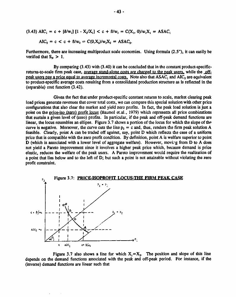
- 43 -

(3.43) AIC, = C + [I/wdJ [1 - X2/XI1 < c + 1/w, = C(X1, 0)/w1X, = ASAC,

AIC2 = c < c + B/W2 = C(O,X2 )/W2 X2 = ASAC2 .

Furthermore, there are increasing multiproduct scale economies. Using formula (2.5"), it can easily beverified that SN > 1.

By comparing (3.43) with (3.40) it can be concluded that in the constant product-specific-returns-to-scale firm peak case, average stand-alone costs are charged to the peak users! while the o.ff-peak users pay a price equal to average incremental costs. Note also that ASAC, and AIC2 are equivalentto product-specific average costs resulting from a consolidated production structure as is reflected in the(separable) cost function (3.42).

Given the fact that under product-specific constant returns to scale, market clearing peakload prices generate revenues that cover total costs, we can compare this special solution with other priceconfigurations that also clear the market and yield zero profits. In fact, the peak load solution is just apoint on the price-iso (zero) profit locus (l3aumol et.al., 1979) which represents all price combinationsthat sustain a given level of (zero) profits. In particular, if the peak and off-peak demand functions arelinear, the locus resembles an ellipse. Figure 3.7 shows a portion of the locus for which the slope of the.curve is negative. Moreover, the curve cuts the line P2 = c and, thus, renders the firm peak solution Afeasible. Clearly, point A can be traded off against, say, point D which reflects the case of a uniformprice that is compatible with the zero profit condition. By definition, point A is welfare superior to pointD (which is associated with a lower level of aggregate welfare). However, moviog from D to A doesnot yield a Pareto improvement since it involves a higher peak price which, because demand is priceelastic, reduces the welfare of the peak users. A Pareto improvement would require the realization ofa point that lies below and to the left of D; but such a point is not attainable without violating the zeroprofit constraint.

P2 Figure 3.7: PRICE-ISOPROFIT LOCUS-THE FIRM PEAK CASE

I4.01~~~*D

I EL

c*/w __ -1X2

AIC2 c _

F.

C AIC1 C+ $/9

Figure 3.7 also shows a line for which X1=X2 . The position and slope of this linedepends on the demand functions associated with the peak and off-peak period. For instance, if the(inverse) demand functions are linear such that

p, =a -bX,,P2 = a - bX2 ,

with a > a and bib, this line is defined by

PI = a - (i/b)(a - P2).

In particular, if 6 = b the line will cut P2 =c at P, = c + a - a. Hence, if the capacitycosts ,8/w, happened to equal the vertical difference between peak and off-peak demand (I - a), theX1=X2 line would go through point A in Figure 3.7. Note also that in this event AIC, = c = AIC2 .In general, though, the Xl = X2 line may intersect the line P2 =c to the left or, which is more likely thecase, to the right of point A. What should be kept in mind as well is that the peak load pricing solution(3.40) coincides with point A only because there are constant returns to scale. Under increasing returnsto scale, for example, the optimal tariff structure results in financial losses and, therefore, does not lieon the price-isoprofit locus.

It is now easy to interpret the firm peak solution in the light of the inequalities (3.43).Any price combination that satisfies the inequalities (3.43) and yields zero profits (i.e. all pricecombinations that lie on the locus segment AB) is subsidy-free across outputs in the sense that bothoutputs dc not require (cross) subsidies to render their joint production financially viable. This is becausethe prices cover at least the incremental costs of producing w,X, and w2X2. Moreover, since the pricesare not allowed to exceed the average stand-alone costs, no output generates revenue that could be usedto subsidize the production of any other output. What then distinguishes point A from, say, point B ?.The answer is that point A rules out subsidies across consumer classes. To see this let the demandfunction be linear, with a > a and b=b. The total net consumer surplus associated with the firm peaksolution is the sum of the net consumer suipluses

NCS, = [a - c - /w1j21/2b and NCS2 = [a - c]2/2b.

We have just shown that (a - a) must be greater than ,B/wI. This implies that NCSI >NCS2, and it also follows that the price elasticity of off-peak demand evaluated at P2 a c is lower thanthe peak demand at P1 = c + #/w. Consequently, raising the price P2 above AIC, and reducing the priceP, below the average stand-alone costs of output 2 not only reduces the aggregate net consumer surplus,but also implies that peak demand will cross-subsidize (in terms of consumer surplus transfers) off-peakdemand. This means that only the firm peak pricing solution is anonymously eguitable. We return tothe concept of anonymous equity in Section 4.2.

What remains to be discussed is the shifting peak case where X, = X2. In this connectionit is helpful to observe that, given the peak and off-peak demand curves, the location of the price-isoprofit:ocus can be regarded as a function of the unit capacity costs. In fact, the higher are the unit capacitycosts, the higher will be the off-peak price at which the price-isoprofit curve intersects the line alongwhich PI=P2 (or XI = X2). Thus, with sufficiently high capacity costs, the shifting peak problem mayoccur. This is depic .ed in the Figure 3.8.

- 45 -

Figure 3.8: Price-Isoprofit Locus - The Shiflling Peak Case

l 2

232 - -

2 -- - -

If, for instance, the price-isoprofit locus is given by er2 = o, the firm peak pricing solutionleads to losses. The correct cost-recovering shifting peak solution will be the price pair p2

2 / p12 for

which X,=X2. Furthermore, with sufficiently high unit capacity costs resulting in the locus ir3 = o, aswitch from a uniform price to an optimal peak and off-peak price structure entails a Pareto-improvement.Both peak and off-peak users will be better off under a shifting peak price regime P3

2 / P, (Baumol,1986). However, the shifting peak solution involves cross-subsidies and, therefore, fails to beanonymously equitable.

Hence, the results of this section can be summarized as follows:

The context of peak load or time-of-use pricing is an example of joint production thatexploits economies of scope from horizontal integration (merit order operation).

Under load-specific constant returns to scale, the single technology firm peak solution(involving the optimal choice of capacity) can be interpreted as an Aumann-Shapley priceallocation that clears the market. This allocation is subsidy-free and anonymouslyequitable.

Under increasing load-specific returns to scale, peak load pricing violates the costrecovery axiom and, therefore, fails to be sustainable without subsidies.

Peak-load pricing maximizes aggregate social welfare, but a switch from uniform to cn-peak/off-peak prices may not qualify as an actual Pareto-improvement.

The shifting peak case occurs if the on-peak and off-peak demand curves lie close togetherand/or the unit capacity costs are sufficiently high. A shifting peak solution is Pareto-optimal, but fails to be anonymously equitable. On the other hand, the shifting peaksituation is necess.-ry for peak load pricing to qualify as an actual Pareto improvement onuniform pricing.

- 46 -

3.2.2 Peak Load Pricing with Diverse Technology

In practice power can be generated with different technologies (heterogeneous plant) ratherthan with a single technology (homogeneous plant). Therefore, let us assume that the availabletechnologies are discrete and can be unambigously ranked in terms of unit capacity and operating/energycosts such that the type of plant with the highest unit capacity costs is least expensive in terms ofoperating costs, and vice versa. In the case of three technologies we thus have

11 < 02 < 03, cl > c2 > c3, and 61+c, >B 2+c 2 > 63+c3.

The above conditions are necessary for a choice of technology to be economically feasible.For instance, if B1 > %2 and cl > c2, the first technology would be economically irrelevant since its usewould always be more costly than that of the second technology.

Given the relative costs of inputs used by the different technologies, the ideal merit orderdispatch can be defined in terms of the rates of usage at which the utility is indifferent between marginalsubstitutions of the technologies. Assuming that the plant-specific rates of usage are fractions of a yearsuch that

WI < W2 < W3 = 1,

the costs of using plant type i will be equal to those of plant type i+ 1 if

Bi + w,ci = 8j+I + wici+,, i = 1, 2.

Solving for the optimal utilization rates yields

(3.44) wI* = [82- 1F]/CI - c2]W* = [113 - 6*]/[c 2 - C3

which implies that

(3.44') n1 = 13 - ,* [c 2 - c3] - w,* [cI -c2J.

Equation (3.44') is the so-called "peaker" pricing formula according to which in an optimally designedsystem the gross capacity (capital) costs of the least capital-intensive plant type should be equal to the netcapacity (capital) costs of the most capital-intensive (or a more capital-intensive) plant type. Net capacitycosts are defined as gross capacity costs, less the savings in operating/energy costs rendered feasible bydisplacing a more capital-intensive plant type.

Now suppose that there are three categories of (price elastic) demand, namely peak load,intermediate load, and base load demand, each with a given rate of usage denoted by wI, w2, and w3,with wI s W2 < W3 = 1 . The demand-related rates w, and W2 may deviate from the technically optimalusage fractions w,* and w2*. So the utility has to decide ab initio whether to install both or only one ofthe plant types that are suited to serve non base-load demand. In addition, it has to select an optimal sizeof each plant type installed. Finally, it has to design an optimal pricing and dispatch strategy for peakand off-peak users.

- 47 -

Again we make the assumption that the different demand function are independent. Thenthe total surplus from installing the three plant types, meeting demand at the levels Xi, X2, and X3, andcharging the prices P,, P2, and P3, can be expressed as

3 X- 3

(3.45) TS = s [w; - wj11] f Pi (X)dX - E Bi [Xi - Xi.,]

Jo

- E wjcj [Xi - X. :1,

where w0 = 0, w3 = 1, and X4 = 0.

In maximizing (3.45) with respect to Xi, the following necessary conditions have to be met:

(3.46) PI = c, + 13/w1 Peak load

P2 = lB2 - B, + w2c2 - w1c11/[w2 - wI] Intermediate load

P3 = [B3 -B2 + C3 - W2C21/1l - WJ Base load

Thus, unlike the single technology case, with diverse techno'ogy, welfare maximization may require thatcapacity costs enter the pricing formulas for off-peak user.. This result which was first derived byWenders (1976) is frequently interpreted as though all off-peak users should always bear part of thecapacity costs if the system is out of equilibrium. What is true is that no capacity charges should beimposed on off-peak users if the system is in equilibrium. In fact, if the optimal usage fractions are equalto the actual rates of usage, (3.46) reduces to

(3.46') P1 = cl + B1/w,* , P2 = c2, P3 = C3.

On the other hand, it is also true that in a disequilibrium all off-peak users shouldcontribute to the recovery of capacity costs if demand is served on the basis of an optimal plant mix. Thelatter condition will be fulfilled if, in particular, the utility is free to choose an optimal plant mix beforeit meets actual or expected demand. To see this, consider the load duration curve depicted in Figure 3.9where the actual (or projected) usage of both peak load and intermediate load is longer than in anoptimum. The curve is based on the assumption that demands are met at the levels XI, X2, and X3 andpower generation is consolidated on the basis of a total capacity X, which can be broken down into (Xl-X2) units of plant type 1, (X2-X3) units of plant type 2, and X3 units of plant type 3. Note that since therates of usage are given, the curve has the shape of a step function where the flat portions reflect theduration of different loads.

- 48 -

Figure 3.9: Load Duration Curve With Given Rates of Usage

kW

xi

x2

X3 -- q -'- - [ I ---

I I !

x4 wl ; w2 4 w 1

Clearly, it is economic to install a peak load plant with size (XI-X2) because w, < WI*.Moreover, the optimal (unit) price charged to peak load users should cover the unit operating costs plusthe peaker plant capacity costs per hour of actual peak load.

It is also economic to install the intermediate load plant with size (X2-X3) because w2 <w2*. Intermediate load prices should bear part of the capacity costs since the savings in operating costsrendered feasible by using the intermediate load plant during the peak period do not fully offset theintermediate load plant's higher capacity costs. Substituting wI*(cI-c2) for (82-71) in the intermediate loadpricing formula, yields

P 2 = [wI-wI*] [Cl - C,2/(W 2 -WlJ + C2 ,

Since w,* > w, and c, > c2, it follows that P2 > c2, i.e. the intermediate load price exceeds the unitoperating costs of the intermediate load technology.

By the same token, the users 0f base load capacity X3 (which is economic to install since w3 > w 2)

should also be charged with capacity costs. Substituting w2*(c2-c3) for (B3-12) in the base load pricingformula (3.46) yields

P3 = 1W2 *-WJ [C2 -c3]/[1-w 2J + C3 > C3 ,

since w2* > w2 and C2 > C3.

However, let us suppose that, for instance, w2* < w2. Clearly, in that case it would beeconomic to substitute base load plant for intermediate load plant and serve both base load andintermediate load demand with base load plant. Such a choice will be feasible at the outset; but once aparticular plant mix is installed, it may turn out that the actual rate of usage, say, of base load exceedsthe optimal one. In this event, base load users should be exempted from (positive) capacity charges. Infact, if w2* < w2, we obtain P3 < c3, i.e. base load users should pay less than the unit base loadoperating costs. One may interpret this "mark off" as a negative capacity charge, accounting for the factthat the savings in operating costs from using base load capacity during the intermediate load period morethan offset the higher base load capacity costs (for a more detailed discussion see the following Section3.3.3).

- 49 -

In sum it can be stated that the conventional peak load pricing model with diversetechnology does not support the claim that in a system disequilibrium off-peak users should routinely berequired to contribute to the recovery of capacity costs. Capacity cost sharing across the users ofdifferent loads may or may not be welfare optimal, depending on the demand curves, the cost functionsassociated with the available plant types, and the installed plant mix.

Finally, let us examine how the solutions (3.46) compare with Aumann-Shapley priceallocations. The cost function from consolidating the production of Xl, X2, and X3 can be written as

(3.47) C(X1, X2, X3) = [B1 -n1Jx1 + E [w1ci-w1.1cjlXj

Obviously, (3.47) exhibits economies of scope. Moreover, costs are separable withrespect to outputs. Therefore, Aumann-Shapley prices are equal to product-specific average costs definedas

8 j-B1 ,1 + w1ci-W*-1ci.i(3.48) ACi = i, = 1, 2, 3.

W., - Wi-i

Bearing in mind that w0 = 0 and w3 = 1, it can easily be verified that (3.48) is equal to (3.46).Alternatively, if we express the solutions (3.46) in terms of stand-alone and incremental costs, it turnsout that the peak load price is equal to average stand-alone costs while off-peak prices coincide withaverage incremental coats. Consequently, the solutions (3.46) are subsidy-free and anonymouslyequitable. Needless to say, the equivalency of marginal cost prices and Aumann-Shapley prices rests onthe assumption that costs are linear in outputs (load-specific constant returns to scale).

3.2.3 Avoided Cost Pricing

In countries like the US or the UK, recent changes in the power sector's regulatoryframework have increased the scope for power supplies from independent, (nonintegrated) nonutilitygenerators. Under these circumstances, utilities have the option (or, as is the case in the US, may berequired) to purchase power from independent producers as a substitute for supplies that the utilitieswould have to provide in the absence of independent producers. This raises the question of what tariffsshould apply to the utilities' power purchases. Purchase taeiffs that are 'too high" may encourage anexcessive amount of independent capacity to be installed and operated, while tariffs that are "too low'may impede the supply of power from less costly nonutility sources.

In this context, the commonly held view is that the appropriate purchase tariffs shouldreflect the costs which the utility can avoid by drawing upon independent power suppliers. In otherwords, the avoided-cost payments should be equal to the incremental costs of producing the amount ofelectricity that could be replaced with supplies from independent generators. Clearly, if evaluated at thelimit, the incremental costs per unit of avoided output will approach the utility's marginal (avoided) costsso that avoided cost pricing would result in the equalization of marginal costs across all producing units(utilities and nonutilities).

The most simple, albeit uninteresting, case is that of a utility which is stuck with excesscapacity. In this situation, the incremental (avoided) costs of a unit of output will be equal to the utility's

- 50 -

(variable) unit operating costs. However, with purchase power tariffs based on operating costs only,there will be hardly any incentive to invest in and run independent generating facilities.

Analytically more challenging is the case where independent generators would displaceadditional investments in capacity which the utility had to carry out in the absence of nonutility powerproducers. Then avoided costs need to be calculated so as to include both operating and capacity costs.While there are a number of practical difficulties of reaching a power purchase agreement in thesecircumstances, our focus will be on a technical problem: With diverse technology, power purchases fromindependent producers undertaken to meet incremental demand may affect the utility's merit orderdispatch. Therefore, avoided costs have to account for the savings or extra costs which accrue from achange in the merit order triggered by independent power supplies. As is shown below, measuring thesecosts may become a complicated task.

In order to develop the generalized avoided cost formula that captures changes in meritorder operation let us first examine the utility's choice of an optimal plant mix relative to a givenmonotonically decreasing load duration curve. For that matter, the subs, 4uent analysis generalizes theapproach used in Section 3.2.2 where the load duration curve was stylized as a step function. It shouldbe kept in mind, however, that the widely used assumption of a given load duration curve is at odds withthe economist's notion of welfare maximization. This is because in determining a welfare maximum, theload duration curve has to be treated as an endogenous variable. Strictly speaking, a continuous loadduration curve must be derived as a continuum of points across a continuum of demand curves fordifferent loads where each point represents a load-specific demand/supply equilibrium. Clearly, inpractical applications the informational requirements of this exercise tend to be forbidding. To simplifymatters, we have therefore assumed in the preceding sections that for each (discrete) load the rate ofusage is given while the load itself depends on price. With a continuous load duration curve, thisassumption is no longer tenable, let alone meaningful (unless demand for each load is price-inelastic).So while a given load duration curve may be derived from power sales observed in the past or mayrepresent the utility's view about the prospective sales during the next billing period, it should not beconfused with a power demand function.

Having these caveats in mind, let us assume, though, that the (annual) load profile isexogenously given by the function F(w) which assigns to each load (kW) a period of time (w) which isexpressed as a fraction of a year. Maximum load occurs at w=O, while minimum load is defined withrespect to w= 1. The special case of a linear load profile is depicted in Figure 10. We also assume thatin serving the given load profile the utility can install up to m=3 different plant types which are indexedin accordance with their merit order such that Bi > Bj and c; < cj for i > j, i, j = I, 2, 3 and .0 = qD= 0, where n denotes (constant) unit capacity costs and c stands for (constant) unit operating costs.Moreover, let X; denot5 the capacity capable of sustaining a load of duration wj, or any smaller load witha duration longer than w1.1, but not exceeding W3 = 1. Then the feasible set of plant mixes withcapacities K;, i = 1, 2, 3, that add up to X, = F(WO) can be defined in terms of condition

3 3(3.49) *E K; E I: [Xj-Xij = XI

with Xi =fF(wi-1) for i = 1, 2, 3|0 for i =4

-51 -

Figure 3.10: Linear Load Duration Curve

kW

x1

x2

-3 F(w)

X4 _------

wnO w w2 w31

Accordingly, for any feasible combination of plant types the total costs of serving F(w) are given by3 3 3

(3.50) C E ~ B Xj+.X] + E C1lwi.lX, - w1X,+11 + E c1H,~~':4 'L:~~ 1 iL:

where Hi = f F(w)dw.JW;,

In view of the load/capacity relationships defined by (3.49), the cost function (3.50) can be rewritten as

-3 .3 3(3.50') C = .E [(8-8.1JFj1 + E wj-I[c-ciJ,Fi. + E ciHi,L=4

where F1 = F(wi.1).

Clearly, in a cost minimum we must have

- = [B1+,-8JF1' + w1[c1+1-cJFi' + [ci+l - cjFi + c,F; - ci+1Fi = 0,

implying that

(3.51) wi* = _ _ , i = 1, 2 .c; - ci+,

(3.51) specifies the necessary conditions for an optimal plant mix in the face of a monotonicallydecreasing load duration curve. Note that the optimal rates of usage wi* are equal to the technicallyoptimal plant utilization rates defined by (3.44) in Section 3.2.2. Also, in the present context the actual,ab initio rates of usage can be adjusted to the optimal levels, whereas in Section 3.22 it was assumed thatthe rates of usage are discrete intervals and, thus, do not necessarily coincide with the optimal plantutilization rates.

- 52 -

By substituting (3.51) into (3.50'), one obtains the load-specific cost functions (note that F;., = X,)

(3.52) C' =1 B;X; + c1H1* for i=1lciH,* for i=2, 3

with E C' = C. Similarly, average load-specific costs can be defined as

(3.53) AC; = B,X,/H,* + c; for i=1i c; for i=2, 3

with E AC,H, = C. Again, it seems that capacity costs should be borne by peak users, while off-peakusers should ae charged with operating costs only. Note, however, that optimal prices would deviatefrom load-specific average costs if each point on the load duration curve - or each hour of the year -represented a distinct demand-supply equilibrium. If spot pricing were feasible, it would in fact clear themarket along the load-specific average cost schedule, i.e. the system lambda curve.

The above results hold as long as the utility is free to choose an optimal plant mix. Oncethe capacity is in place, however, the capacity costs are sunk because the utility has no or only limitedopportunities to disinvest. Consequently, in responding to a shift in the load duration curve the utilitywill be stuck with capacities installed in the past and, thus, may not be able to retain an optimal plantmix.

To see this, consider an outward shift in the load duration curve, with incremental demandbeing equal to AF(w). Depending on the nature of the incremental demand function, the shift will be

- neutral, if the load increments do not vary with w,

peak-biased, if the increments decrease with w, and

- base-biased, if the increments are an increasing function of w.

Hagen and Vincent (1989) argue that an equilibrium cannot be maintained if, and only if, the outwardshift in the load duration curve is base-biased. In our context, this result can be demonstrated to holdas follows:

If F(w) denotes the new load duration curve while K, represents the size of the i-th plant installed, thenthe cost function (3.50') has to be minimized subject to the constraints

(3.54) Xi - Xi, - Ki 2 0, i = 1, 2, 3,

where Xi is defined as in (3.49). Condition (3.54) states that disinvestments are not feasible, i.e. inserving the new load profile the utility cannot reduce the size of existing plant (unless the age of old plantmakes its use economically obsolete, a case which we neglect for the sake of convenience). As a result,the necessary conlitions for a cost minimum can be rewritten as

B, - f,+- w,lc,+, - c,j = cxi

- 53 -

so that

(3.51') w; = + ,= 1, 2Ci -ci+

where a; denotes the Lagrange multiplier associated with the i-th capacity constraint. Clearly, themultiplier a; measures the extra costs which would be incurred at the operational margin if plant type iwere in place of plant type i+ 1. Stated differently, a, is equal to the difference between t.e gross capitalcosts of a unit of plant type i and the net capital costs of a unit of plant type i+ 1 that is operated at themargin. Therefore, a positive a; implies that a unit of plant type i+ I is worth less than a unit of planttype i. Also, we have a, > 0 (=O) if the i-th constraint is binding (not binding). It is also obvious thatall constraints will be binding if, and only if, the load shift is base-biased. By the same token, a base-biased shift in the load profile will cause any plant, except the most capital-intensive one, to be used ata rate exceeding the optimal utilization level. In fact, it follows from (3.51) and (3.51') that

w; = [1 + a,/(fli+, - 83)] w,* , i = 1, 2

implying w; > w,* since fli+I > B;.

kW Figure 3.11: Base-Biased Load Shift

x

X3

X4 . .W 1 W2 w2

Figure 3.11 illustrates a base-biased shift in the load duration curve (from F° to F') where no capacityadditions are warranted since the level rf peak-load remains constant. The figure suggests that it maybecome profitable to entirely sink (i.e. scrap) the capacity costs of a plant already in place and to installa plant type with higher unit capacity costs resulting in lower unit operating costs. In fact, the utility willbe indifferent between using a unit of plant i and replacing it with plant i+ 1 if the (annuitized) capacitycosts of the new unit plus the (annuitized) sunk costs of the old plant (which can be considered asfinancial committinents made in the past) are equal to savings in operating costs rendered feasible bydisplacing of the old plant, i.e. when

Bj+, + 8, = w; [c; - ci+,], with w,* < w; S 1.

- 54 -

where %, denotes the critical utilization rate. Thus, if the load shift causes w; to exceed vi, thedisplacement of plant type i becomes a profitable option. It should be noted that the same effect mayoccur as a result of a change in relative input prices associated with the different technologies. Tosimplify matters, though, our analysis will be confined to disequilibrium configuration brought about bya shift in the load duration curve.

Substituting (3.51') into (3.50') gives the load-sDecific cost function resulting from a base-biased shiftin the load duration curve, i.e.

(3.52') C' = (BX, + c,Hi for i = 1(c,H, - a,., Xi for i =2, 3

Thus, peak-load demand will be charged with peak-load capacity-plus operating costs, while off-peakusers have to pay the operating costs incurred during the respective off-peak period i = 2, 3, less theextra costs which would occur at the operational margin if capacity Xi were provided by the !loss capital-intensive, but more-costly-to-operate plant type i-l.

Accordingly, the value of a unit of base load capacity is equal toB1, - a2 - aX1,while a unit of intermediate load capacity is worth1B, - a,.

Moreover, let Hi* denote tha areas under the load duration curve associated with optimalplant utilization rates wi*, i = 1, 2. Then the difference between total out-of-equilibrium costs and thecosts which would be incurred under an optimal plant mix works out at

(3.55) C(F) - C(F*) = E c,[H, - Hj, - :a , Xi

Thus, the cost differential is equal to

the difference in operating costs, net of

- the extra costs which, at the operational margin, would accrue from a switch towards aless-expensive-to-operate (but more capital-intensive) plant mix.

In view of the above observations it is now easy to define what are the costs that a utilitywill avoid if part of a load increment is served by an independent power producer. Let there be anoutward shift in the utility's load dutation curve from F° to Fl. If part of the load increment, say, F' -F2 is served by an independent producer, the utility's avoided costs can be expressed as

(3.56) AVOC = C() -C ) 3

= 8,AX, + c.c,&H. - E aii. (F')Xi'+ a1 (F),b"1 A2.&:

where &X, - Xi ' - X ,AH;- Hi' - H2,

- 55 -

and C(F') represents the minimum costs of serving Fi. Thus, avoided costs are equal to the differencein costs that the utility would face in the absence and in the presence of independent power production.The rationale underlying the avoided cost formula is that the utility will be indifferent between purchasingthe electricity needed to serve F' - F2 and paying C(F') - C(F) to the independent producer on the onehand, and, on the other, generating the same amount of electricity at additional costs C(F') - C(P).

The advantage of formula (3.56) is that it considerably simplifies the line of argument putforth by Hagen and Vincent (1989). In fact, formula (3.56) covers the following constellations:

CaeI: a(F') = c(i 2) = O, i = 1, 2

In this situation Equation (3.56) reduces to3

(3.56') AVOC = n,AX,* + E c,AHi*

so that avoided cost pricing is equivalent to peaker pricing as proposed by Joskow (1982). Therefore,the utility should pay the avoided operating costs plus the unit capacity costs of the peaker plant type foreach avoided unit of off-peak capacity. Note that under constant returns to scale exactly the samepayments will be obtained from average cost pricing.

Case II: &.(F') = ati(17) > 0, i = 1, 2

In this case where the shift in the load duration curve is base-biased, independent power production doesnot amplify or mitigate this bias. Consequentlv, (3.56) can be rewritten as

3 .(3.56') AVOC = 81A,X + E ci AHi - E ax., *Xi,

implying tihat out of equilibrium a unit of off-peak capacity is worth less than the capacity costs of a unitof peaker plant. Hence, the peaker pricing method would entail overpayments to the independent powerproducer. Case studies conducted by McKechnie (1985) show that the difference between peaker pricingand a correct out-of-equilibrium cost estimate may be substantial.

Case III: a&(F) > aj(F') 2 0, i = 1, 2

In this case, the independent producer's supply is peak-biased and results in a more base-biased load duration profile served by the utility. Therefore, the payment to the independent producershould be less than under a peaker pricing remuneration scheme or, what comes to the same thing, apricing scheme based on equilibrium average costs.

Case IV: aj(F') > cei(F) > 0, i = 1, 2

The above constellation implies that the independent producer's supply is base-biased.Two cases may occur. If cxi(F2) = 0, the utility saves more than equilibrium average costs. On thisscore, peaker pricing would lead to an underestimation of avoided costs. On the other hand, if o0(F2) >0, the avoided costs may be greater, smaller than, or equal to the payments that would result from thepeaker pricing method. This is because the savings from the reduced overutilization ef plant renderedfeasible by the independent producer's supply may be greater or smaller than, or may be just offset by

- 56 -

the extra costs involved in the disequilibrium (i.e. suboptimal plant mix) to which the utility remainsexposed notwithstanding the supply from independent producers.

The following points should be reemphasized:

First, in determining the utility's avoided costs there is no need for specifying or knowingthe technology used and costs incurred by the independent power producer. A profit maximizingindependent producer will supply electricity to the point where marginal revenues are equal to marginalcosts. Since marginal revenues are required to be equal to the utility's marginal costs savings (which maybe positive or negative), avoided cost pricing will equalize marginal costs across all producing units. Ifthere were no supplies from independent producers (if only because avoided cost-pricing would leaveindependent producers with losses), the same result would hold.

Second, avoided cost nricing presumes that prices are set on the basis of the utility's costs.Final consumers are charged with the same rates they would have to pay if the utility had not purchasedelectricity from independent producers. All savings or increases in utility's costs resulting from theindependent producers' supply are internalized by the independent producers, rather than passed on tofinal consumers. For instance, cost savings are captured by the independent producers in the form ofhigher profits. It has therefore been argued that avoided cost pricing is economically inefficient (Woo,1988). This objection is valid if the utility would set prices above marginal costs (e.g. because MC-pricing, due to economies of scale, is doomed to entail financial losses) and demand were sensitive toprice changes. In the preceding analysis we have assumed these complications away by ruling outincreasing returns to scale and treating the load duration curve as a given. Note also that we disregardregulatory impediments which require the utility to use suboptimal pricing strategies.

Third, we have shown that the utility's average (load-specific) costs may change as aresponse to an outward shift in the load duration curve even when relative input prices remain constantand there are constant returns to scale. This is because with irreversible investments, the utility may notbe able to retain or attain an optimal plant mix. In such a situation the principle of avoided cost pricinghighlights the fact that pricing rules based on single product analogies or multiproduct equilibriumconfigurations generally are misleading.

3.2.4 Capacity Cost Responsibility in the Face of LOLP

The rule that the entire capacity costs should be borne by peak-load users has severalexceptions. For instance, it has been shown in the previous sections that it may be efficient to chargeoff-peak users with capacity costs if the system is saddled with a suboptimal plant mix. There is, though,another argument which can be raised in favor of an allocation of capacity costs across different loadseven when the system is in equilibrium. The argument draws support from the fact that in practice itcannot be ruled out that at any time of the day, month, or year demand must be curtailed due to outagesof generating units. (To simplify matters, we disregard curtailments of electricity supply resulting fromtransmission and distribution failures.) Consequently, it may happen that peaker plant will be used toserve off-peak demand. This suggests that off-peak demand should share some of the capacity costs (see,for instance, Vardi et.al, 1977 , and McKechnie, 1985).

To illustrate the argument let us consider an optimal mix of three homogeneous generatingunits of uniform size, each with an outage rate of 5%. Generally, with n units, there will be 2"outage/availability combinations. In the simplified case in question, however, the number reduces to n+ I

- 57 -

combinations. As in the previous section, peak, shoulder-peak, and base-load capacity are denoted byXI, X2, and X3. Their availability depends on the outage probabilities. For instance, the probability thatthe peaker capacity is available amounts to (1-0.05)3 - 0.857. Moreover, let us conceive outages as anadditional demand for capacity that is not available. For instance, if one of the units is not operational,the additional demand is equal to X3, and total demand works out at Xl + X3. By the same token,outages can be regarded as an outward shift in the load duration curve (subject to the caveats mentionedin Section 3.2.3). The resulting "composite' load duration curves are depicted in Figure 3.12. Forexample, F, applies if the total installed capacity is available with probability 0.8574, while F4 refers tothe case where the total available capacity is zero with probability 0.0001.

Figure 3.12: Composite Load Duration Curves

0.001

#0.0024

XI N. ~F

installedcapacity X2 -i

X3

The horizontal line through the total installed capacity X, intersects the different compositeload duration curves at points that correspond to capacity utilization rates w; (fractions of a year) thatsubdivide the total billing period (I year) according to outage probabilities. In the special case underconsideration, these rates coincide with the optimal capacity utilization rates w3* determined by theoptimal plant mix since the generating units have a uniform size. In general, however, the number ofperiods determined by the outage probabilities will be greater than the number of load-specific utilizationintervals that would prevail in the absence of the risk of outages. In this respect, McKechnie (1985) isright in arguing that 'the traditional distinction of peak and off-peak is artificial in a world of (supply)uncertainty" (p. 17).

As is shown in Table 3.1, the outage probabilities A., i = 1, 2, 3, are symmetric to thecumulative occurrence probabilities of available capacity. What becomes obvious as well is that theoutage probability ui can be interpreted as the probability that capacity which in the absence of outageswould not be used in period z; = w; - w ,1, i = 1, 2, 3, w. = 0, will be called into operation duringperiod z;. Accordingly, ziui, which is the so-called loss-of-load probability (LOLP) associated with periodz;, can be viewed as the capacity cost responsibility of period z;. In the special case under considerationwhere the optimal rates wi* (at 100% reliability) are equal to wi, the purist's distinction between peak,intermediate, and base-load remains valid. Therefore, the principle of capacity cost responsibility impliesthat in the face of supply uncertainties off-peak users should share some of the system's capacity costs.Stated differently, peak load demand should no longer be charged with the entire capacity costs.

- 58 -

Table 3.1: Example of Outage Probabilities*

Available Probability of Cumulative Outage Length of CapacityCapacity Occurrence Prob. of Occ. Prob.(u;) Period(z;) in Outage

XI 0.8574 0.8574 0.1426 z,=w1 0X2 0.0451 0.9025 0.0975 Z2 =W2 -Wl X3

X3 0.0024 0.9049 0.0951 z3 =w3-w2 X20 0.0001 0.9050 0.0950 Z4 W3 XI

* homogeneous generation units of uniform size, each with an outage probability of 0.05.

Under the assumptions made in this section, capital cost apportioning relative to the outageprobabilities is a straightforward exercise. The system's LOLP, defined as the cumulative expectedduration of disruption in supply, is given by

3 3LOLP = E LOLP1 = E zu;,

where LOLP; denotes the loss-of-load probability for the i-th load interval. Thus, B,/LOLP is the lastpeaker unit's capacity costs per expected hour of operation per year. Substituting the responsibilityfactors

(3.57) R; = LOLP3/LOLP, i = 1, 2, 3

into (3.52), Section 3.2.3, yields

(3.58) Ci = B1X1R1 + cH., i = 1, 2, 3.

Thus, capital costs will be allocated across load intervals so as to reflect the outageprobability distribution over the total billing period. Obviously, the shares in the systems capital costsincrease along the merit order dispatch.

It should be noted, however, that in general the merit order determined by the outageprobability distribution will differ from that obtained in the absence of supply uncertainties. This impliesthat in general capital cost responsibility pricing leads to a departure from the peaker pricing principle.

What should be kept in mind as well is that in practice the level of LOLP is a pretermineddesign criterion for cystem planning. So it is the LOLP target (e.g. 1-day-in-10-years LOLP) whichimplicitly determines the outage probability distribution, the total installed capacity and, thus, the capitalcost responsibility associated with different load intervals. Clearly, the choice of a higher or lowerreliability target should be subject to economic considerations. In particular, the more reliable is thesystem, the more expensive will be the electricity that an additional generating unit can be expected toproduce, and the higher must be the willingness to pay to justify the increase in reliability (for a moredetailed discussion, see Telson, 1975). Moreover, once outages occur, the principle of capital cost

-59 -

responsibility will not ensure that outage costs are allocated efficiently. In fact, the efficient allocationof outage costs is an entirely different matter that has to be dealt with in the short-run, as opposed tolong-run adjustm,ents in plant mix and reserve margin. Ideally, spot pricing would be the most efficientapproach to rationing power supplies during shortfall situations. Technological limitations and prohibitivetransaction costs, however, may render spot markets difficult to establish and operate (see the followingSection 3.2.5). An alternative way of allocating outage costs is to offer priority service schemes thatallow customers to choose a merit order of being served (see, for instance, Wilson, 1989). Section 5.3provides a more detailed discussion of the priority pricing approach.

3.2.5 Real Time Pricing

In the conventional time-of-use pricing model (Section 3.2.1), optimal capacity and tariffsare selected ex ante; and since it is assumed that supply and demand can be predicted with certainty, thereis no need to revise the level and structure of tariffs ex post. In practice, however, both supply anddemand are stochastic and, thus, may not equalize. So if tariffs are predetermined, excess demand needsto be rationed through (indiscriminate) load shedding or voltage reductions once supply falls short ofdemand, while capacity 'will be idle in slack periods. Ideally, a more efficient allocation of services couldbe achieved by continuously adjusting the level and structure of tariffs so as to equate demand with supplyover time. This approach is known as "responsive pricing" or "spot pricing". Clearly, in the powersector, spot pricing amounts to instantaneous time of use pricing or, what comes to the same thing, "realtime pricing".

A simple example will suffice to highlight the rationale underlying the concept of spotpricing. (For a more comprehensive discussion of spot pricing in the power sector see Bohn et.al.,1984). Let us assume that at any point in time demand for electricity, X, is a function of price, p, andan independent, identically distributed random variable, e (e.g. temperature). Supply is certain (100%reliability), but constrained by the capacity installed in the past, i.e. X 5 K. Moreover, there areconstant unit operating and capacity costs, denoted by c and B, respectively.

Let E denote the expectation operator. The expected consumer surplus CS is given byx

(3.59) E{CS} = f I f p(x,O)dx - px)f(e)de,

)e Joand the expected profits can be expressed as

(3.60) E {ir) = f [p(x,e)-cJX) f(O)dO - BK.

Jo

It is assumed that the utility knows the consumers' preferences and the distributionfunction of 0, denoted by f(O). Moreover, the utility is committed to maximize the total expectedsurplus E{CS) + E(T) by [11 choosing the capacity ex ante and 121 setting the price ex post, dependingon the realization of 0 and subject to the capacity constraint. Clearly, the optimal choice of capacity (exante) and spot price (ex post) has to satisfy the conditions

(i) X[p-c-a 0 , p-c-ca 0

- 60 -

(ii) a[K-XJ= 0 ,K-X 2 0

(iii) K[a-8] = 0 , a-8 5 0,

where a is the Legrange multiplier associated with the capacity constraint. The above conditions implythe following decision rules:

- The capacity choice should be such that the expected price covers "long run marginalcosts", i.e. E{p*} = c + B.

- If there is excess capacity, the spot price should be equal to short run marginal costs, i.e.p* = c.

- If the capacity constraint is binding, the spot price should be set so as to bring demandin line with supply, i.e. [p*-c]X(p*) = BK.

As is easy to imagine, the analysis can be extended to cover a system with diversegenerating technology. In this more general setting, efficient spot prices would follow the system larmbdacurve reflecting the merit order of load dispatch. Likewise, one could take account of loss-of-loadprobabilities in which case the expected price would exceed long run marginal costs. At any rate, theline of argument advanced in favor of spot pricing does not break new ground. In essence, spot pricingboils down to continuous time peak load pricing defined in the face of stochastic demand and supply.

What comes somewhat as a surprise, though, is the recently awakening interest in thepotential for spot pricing of electricity (see, for instance, Weyman-Jones, 1988, and Sioshansi, 1990).It seems that the optimum optimorum referred to by the concept of real time pricing often serves as aromantic retreat for policy makers and energy planners dissatisfied with the inefficiencies of real worldtariffs. That is to say, one should not become oblivious to the institutional and technical difficulties thatare likely to hamper the implementation of efficient spot prices.

One shortcoming is that the utility has no incentive to follow the decision rules for optimalspot pricing. In particular, if SRMC-pricing were called for, the utility could gain (windfall profits) fromfalsely asserting that price should be set above SRMC. So without a perfectly informed regulatoryauthority that is in the position to compute and enforce optimal spot prices, the utility cannot be expectedto perform as though there were efficient spot markets. It has therefore been argued that due to theinformational restraints impairing the regulator's ability to control the utility, it would be more effectiveto horizontally disintegrate the industry into several generating companies that compete on price in thestyle of Bertrand oligopolists (Littlechild, 1988). As the UK-experiment on power sector restructuringshows (Green and Newbery, 1991), however, the generation capacity must be split among a large enoughnumber of suppliers to render a Bertrand MC-equilibrium feasible. Otherwise the conditions will beconducive to non-competitive pricing strategies that may end up in tacit collusion (Tircle, 1989).

Be that as it may, for power to be traded and priced in spot markets, an auctioneer willbe indispensible. Centralized dispatch, executed by an independent (regulated) transmission entity inaccordance with the suppliers' bids, would be a solution to this problem, provided the bids are placedin such a way that their ranking conforms with the system lambda curve. But there also are formidabletechnical obstacles to the implementation of instantaneous time-of-use pricing. What would be requiredis an information system that

-61 -

- unveils and monitors the consumers' perferences,

- facilitates a two-way communication between power generators, the transmission network,and the distributors/consumers, and

- includes a central unit capable of handling and processing the various flows ofinformation.

Sophisticated and affordable technologies that meet the requirements for metering,monitoring, billing, etc. and rendcr the communication and management of a huge amount of datafeasible, will not be available in the forsecable future. And even if these technologies could beimplemented at reasonable costs, many customers might find it impossible, too expensive, or notworthwhile to respond to the signals and service options that spot markets are supposed to provide. Atleast, there is no a-priori evidence that complex spot pricing would be considerably welfare superior toless sophisticated time-of-use pricing. Finally, if marginal costs lie below average costs, strict real timepricinig creates the same financial problems on account of which Ramsey pricing or other rules departingfrom the principle of MC-pricing can be justified. For that matter, real time pricing will not be immuneagainst challenges posed by "second-best" or "third best" reasoning.

In short, real time pricing (spot pricing) is a "high-end" variant of MC-pricing. It iscontingent on the availability of sophisticated information technologies and requires an industry structurethat permits electricity to be auctioned off. It remains to be seen whether and to what extent real timepricing, should it become practical, will outperform less ambitious pricing strategies. This will dependon (i) the intrusiveness of uncertainty, (ii) the transaction costs of acquiring and digesting a huge amountof information, (iii) the scope for, and gains from, a competitively driven merit order dispatch, and (iv)the presence of diverse and responsive demand.

4. Linear Break Even Pricing

If marginal cost pricing leads to financial losses and the utility is required to break evenwithout receiving any subsidies, there is no way but to charge discriminatory tariffs (which, by definition,depart from marginal costs). In the present chapter the focus is on (discrimil ;tory) linear prices thatrender the utility financially self-sufficient. Linear (or uniform) prices do lot vary with the kWhsproduced/sold/purchased, as opposed to nonlinear prices which will be discussed in Chapter 5.

The analysis of linear pricing rules is confined to two special cases: Ramsey prices whichare second-best, and so-called sustainable prices which, if they exist, rule out profitable entry in marketsserved by the utility. It is shown that Ramsey prices are not necessarily sustainable. In addition,attention is given to the idea of price cap constraints which under certain conditions may induce aniterative process that converges to a Ramsey-optimal solution.

4.1 Ramsey Pricing

As is well known, if the principle of cost recovery requires the utility to depart from MC-pricing, and given the restriction that nonlinear pricing strategies are not feasible, then the second-best(partial equilibrium) solution calls for linear Ramsey prices (see, for instance, Baumol and Bradford,

- 62 -

1970). In this context second-best means that the utility maximizes the sum of the consumers' andproducers' surplus subject to the break-even constraint. This is equivalent to minimizing the deadweightlosses resulting from a departure from MC-pricing. To illustrate the problem recall the diversetechnology model discussed in Section 3.2.2. The utility has to serve peak load, intermediate load andbase load demand which are assumed to be independent. Moreover, let the unit capacity costs of thedifferent plants be a decreasing function of the capacity size. As in Section 3.2.2, the objective is tochoose a plant mix and a set of prices such that the total surplus given by Equation (3.45) is maximized.In the present setting, however, the maximization problem is constrained by the condition that totalrevenues at least cover total costs, i.e.

3 31 [w1 - wi 11 Pi(X)Xi - E C'(X) a 0.

As can easily be "erified, a welfare maximum has to satisfy the necessary conditions

- lCi 1t a (4.1) Pi- - -- -' i = 1, 2, 3

Ui; [W; - Wj,]l (I+&) e;

_Pi

where e; = -(PI/X;) (ZX1IAP;) denotes the price elasticity of demand and a is the Lagrange multiplierassociated with the break-even constraint. The term a/(I +a), the "Ramsey number", is zero if thebreak-even constraint is not binding (constant returns to scale). If the constraint is binding, the "Ramseynumber" cannot exceed unity (monopoly pricing); so it may happen that there is no set of linear Ramseyprices that allows the utility to break even.

The left hand side of condition (4.1) measures the relative mark-up of price over marginalcosts and is inversely proportional to the price elasticity of demand. The more inelastic is demand, thehigher should be the mark-up (inverse elasticity rule). Thus, Ramsey pricing discriminates acrossoutputs. And if, as we have assumed, the different demand curves arc independent, there will also bediscrimination across consumer (load) categories.

With an optimal plant mix, (4.1) can be written as

(4.1') PI - cl - 61/w, - (38,/aX,) (1/w,) a I------------------ --- - (Peak)

Ph l+a e,

a 1(Pi -c)/P= --- , i = 2, 3 (Off-Peak)

I+a e;

Thus, unlike the peak load pricing solution (3.46'), Ramsey pricing, pursued under a binding break-evenconstraint, implies that off-peak tariffs exceed the level of the respective (constant) unit operating costs.If the break-even constraint is not binding, however, (4.1') boils down to the conventional peak loadpricing rule which is equivalent to the principle of average cost pricing if the utility's cost function is,as has been assumed, separable with respect to different loads.

- 63 -

Moreover, the Ramsey formula can easily be extended so as to account for social weightsattached to different consumer classes. For instance, if for social considerations the (net) consumersurplus of the i-th consumei class should not fall below a predetermined level, say, CS,', then totalwelfare must be maximized subject to the additional constraint

CS, 2 CS,° .

In this case the Ramsey nmmber for output i amounts to (ct-)/(l+qa) where 6b is thelagrange multiplier associated with the i-th surplus constraint. Consequently, if the i-tb surplus constraintis binding there will be a downward pressure on the i-th mark-up, while the mark-ups for the remainingoutputs are pushed upwards in order to recover the utility's costs.

Three observations can be made:

First, Ramsey prices, if they exist, will fully distribute the utility's costs across outputs. However, itshould be kept in mind that the allocation of costs is implicitly determined by the Ramsey pricing solutionand, thus, does not fol'ow an a-priori formula for the apportioning of (fixed) costs.

Second, in order to deduce the Ramsey solution one has to know the demand functions (unless returnsto scale are constant). Thus, when there is no information aoout the consumers' demand, second-bestpricing becomes an elusive goal.

Third, the inverse elasticity rule (4.1) has been derived by assuming (as in Chapter 3) that the load-specific demand functions are independent. Unlike compensated demand functions, this assumption doesnot necessarily hold for ordinary (Marshallian) demand curves on which our approach to measuring theconsumers' surplus has been based. The reason for this is that line integrals over curves inmultidimensional space in general are path-dependent, i.e. depend on the path that connects the curves.Economically speaking, this means that a change in the (uncompensated) demand for output i resultingfrom a change in the price of output j may be biased by income effects. The assumption of demandindependence requires that income effects are absent, i.e. that the cross-price derivatives of any twodemand functions are symmetric. While this assumption cannot hold economy-wide (otherwise the budgetconstraint would be violated), it may be justified for a subset of demand functions (e.g.telecommunications, electricity). For instance, one can expect that the demand for a long-distance callto city XI is not very sensitive to the price of a phone call to city X2. In the power sector, however, peakload demand may very well depend on the price charged to off-peak demand. In this event the inverseelasticity rule has to be modified so as to account for cross price effects (see, for instance, Crew andKleindorfer, 1986, pp. 18-21). In particular, if two outputs, say peak load and base 'oad, arecomplements, may happen thst one output needs to be priced below MC. Nonetheless, formula (4.1)provides a reasonably accurate approximation to a second-best pricing rule if substitution effects proveoverwhelming'v large relative to income effects (across the oLt1puts provided by the electric utility).

Be that as it may, the relevance of the Ramsey-pricing rule has frequently been questionedeither because the utility does not seek to maximize social welfare or because a regulatory authority whichis required to enforce Ramsey prices has little or no knowledge about the utility's cost and demandfunctions. Moreover, in a regulatory setting Ramsey pricing would come close to a (marginal) cost plus(zero profit) concept that fails to provide the utility with an incentive to cut costs. These problems haveprompted the question of whether utilities can be induced to adopt Ramsey-optimal pricing strategies

- 64 -

without an explicit or implicit commitment to the principle of welfare maximi7ation. An interestinganswer to this problem is the linear Brice capping approach.

The idea of price caps has been developed as a regulatory means of divorcing prices fromcosts. While there are different variants of price cap regulation, the common feature of price caps is thatthey dismiss the traditional concept of profit regulation and allow the utility to do what it likes (which,in an ideal world, would be to maximize profits by cutting costs) as long as it does not raise prices abovea fixed or indexed level. Furthermore, in setting and monitoring these price ceilings the regulator is notsupposed to have complete information about the utility's cost function and the consumers' preferences.

In this context, the behavioral assumptions underlying the linear price capping approachcan be considered as a case of reversed Ramsey pricing. In fact, let us assume that the utility maximizesprolits subject to the constraints that

- only uniform prices are feasible, and

- the aggregate (net) consumer surplus does not fall below a predetermined level, say, CS'.

Using the diverse technology model presented in Section 3.2.2, the problem can thus be stated as3 3

(4.2) Max E [w1-w-11 Pj(X)Xj - E CQ(X) S.T. CS 2 CS'

where CS = t[w1-w1.dl f Pi(X)dX - E PiX;4=i 1J A:I

(Note that in (4.2) tile demand functions are supposed to be independent). In a profit maximum, thenecessary conditions to be met are given by

pi - (8Ci/bx;) (1/Z,)(4.3) ------ (l-a)/e;, i = 1, 2, X

pi

where e; denotes the i-th price elasticity and ca is the Lagrange multiplier associated with the surplusconstraint. The term Z; stands for w1-w1 , and will be neglected henceforth.

As with Ramsey prices, the mark-ups will be inversely proportional to the (upwardadjusted) elasticities of demand. Also, (4.3) implies monopoly pricing if a=O. And for a= 1 prices arerequired to be equal to marginal costs.

Now let us assume that the surplus constraint renders non-negative profits, say, 1' ! 0feasible. Then the necessary conditions (4.3) would also apply if the utility were to maximize the netconsumer surplus subject to the profit constraint ir 2 7r'. Alternatively, one could permit the utility tomaximize profits subject to the constraint that prices do not exceed the levels determined by (4.3).

Unfortunately, in practice the utility cannot be expected to explicitly maximize welfare;nor will a regulator be in the position to compute and impose the set of tariffs which in a profit maximumwould yield the desired level of aggregate consumers' surplus. However, what a regulatory authority cando is to consider a particular set of prices (e.g. the currently prevailing prices) as "socially acceptable".

-65 -

In this case it would be a kind of minimum welfare requirement not to allow the utility to alter the pricestructure if this change would result in a level of aggregate consumer surplus lower than that implied bythe socially acceptable set of prices. One may argue that there is no way of measuring the change in theaggregate consumers' surplus induced by a change in prices. Computing these changes, though, isamazingly simple. In fact, a marginal departure from the socially acceptable price structure will notreduce the level of aggregate consumers' surplus if

.3 acsi 3(4.4) dCS = - dp; E X,dp; > 0.

4:1 api i-1

Note that the price-cap condition (4.4) does not exclude the possibility that a consumer class will be betteroff at the expense of another one. So condition (4.4) is only potentially, but not actually Pareto-optimal.It rules out that the consumers will be worse off in the aggregate.

Clearly, in practical applications where changes in prices are discrete rather thancontinuous, condition (4.4) needs to be approximated. Therefore, suppose that a change in the i-th price,i.e. Ap; = pit-pi' leads to a change in output from XN. to Xi'. Then the change in the aggregateconsumers' surplus will depend on whether the weighted average of the change in prices is expressed interms of previous period (pre change) quantities Xi' or current period (post change) quantities Xi'. Thisis equivalent to using a Laspeyres or a Paasche price index. If a Laspeyres index

_r X; P;/r X; P;j (2 1)

is applied, condition (4.4) can be approximated by

(4.5) ACS -I X,0[Pi1 - PiJ] 2 0a-1

from which it follows that3 3E P°0 X3

0 > E Pit Xi'.

Thus, condition (4.5) requires the Laspeyres price index not to exceed unity. By standard revealedpreference arguments (see, for instance, Varian, 1987, pp. 124-129) this implies that consumers will notbe worse off. (Note that income effects are assumed to be zero or negligibly small). Anotherinterpretation of the index condition is that the utility is allowed to choose a set of prices which, ifweighted by the last period's output, would at best generate the last period's average revenues.

Moreover, it can be shown that under certain conditions a price-cap regulated profitmaximizing utility will opt for a time path of prices and outputs that converges to a Ramsey optimum.To see this consider the single period constrained profit maximization problem

3Max 7r./X)) = E P; X;1 - C'(X1)

3S.T. E Pi0 Xi" - Pj1(X')X1

0 > 0

The necessary conditions to be met in a maximum are

- 66 -

Pi' JC'/bX aXyj 1(4.6) --- = [1 - ---- , i = 1, 2, 3,

pil Vj f

where ef is the price elasticity evaluated at Y.,. (Note that we neglect the term Z; = w,-wi l thatappears in Equation (4.1)). Thus, if the Laspeyres index constraint is not binding, i.e. if a = 0, theconditions (4.6) call for monopoly pricing. In this event the utility has no incentive to alter theprevious oeriod prices. On the other hand, if 0 < a s 1, the price cap requires the profitmaximizing utility to act as diough demand were more elastic. Furthermore, if Xj' = XY, and, thus,Pi' = Pi', (4.6) reduces to the Ramsey solution (4.3).

Now suppose that (4.6) differs from (4.3). Then price capping will induce aniterative process whereby in each period the quantities produced/sold in the previous period are usedto calculate the Laspeyres price index constraint. In the sin le product case it is intuitively plausiblethat this process will converge to the solution (4.3). This is because profits can only be increasedthrough a higher output sold at a lower price so that v, utility will move along its decreasingaverage cost curve. Brennan (1989) has shown that the same result will hold in the multiproductcase provided that the utility's cost and demand functions are stationary (in addition the assumptionof independent demands and the use of a Laspeyres index).

In the light of the convergence properties of the price capping mechanism it becomesobvious that once a set of prices is considered "socially acceptable", the implied level of utilityprofilts qualifies as "appropriate" or "just and reasonable". Then price capping induces the utilityto eventually choose a set of prices and outputs that maximizes the consumers' surplus relative tothe "appropriate" level of profits. Clearly, if a regulator knew the cost and demand curves at theoutset, he/she could require the utility to immediately move to the Ramsey optimum. If not, theprice capping is a means of shifting the workload of welfare optimization to the utility.

Several remarks are in order:

First, everything being equal and assuming that the utility's multiproduct cost function exhibitsdecreasing ray average costs (see Section 2.3), the price capping mechanism will ultimately resultin a zero-profit Ramsey optimum (4.1), if in every period the utility's choice options are restrictedto prices that would at best result in zero profits if the output bundle sold would be that of theprevious period (Vogelsang and Finsinger, 1979).

Second, using a Paaschie price index constraint will not ensure that the utility approaches a Ramseyoptimum. Moreover, a Paasche index requires forecasting of outputs, while the Laspeyre index canresort to observed outputs.

Third, disproportionate changes in demand for the different outputs require the regulator to knowcurrent demand in order to select the correct quantity weights. Moreover, by (correctly) anticipatingthe changes in demand the utility may exploit this informational advantage at the expense of theconsumers' surplus (Brennan, 1989).

- 67 -

Fourth, in practical applications (e.g. British Telecom) the price index constrainm. is often amendedby a "retail/wholesale/consumer price index minus X" formula. For instance, in the case of "RPI-X", the price constraints are multiplied by the difference between the retail price index and theexpected productivity gains.

Fifth, a Ramsey optimum based on linear prices may not exist so that nonlinear p,.cing strategiesare called for. In this case price caps can be implemented in the form of constrained optional multi-part tariffs. This issue will be discussed in Chapter 5.

Sixth, welfare improvements generated by price caps of the form (4.5) depend on the assumption thatthere are no income effects.

Seventh, the choice of base period prices should not be left to the utility because they determine thelevel of profits relative to which the consumers' surplus will be maximized.

4.2 Sustainable Prices and Efficient Industry Structure

The notion of sustainable prices has been developed in the context of the contestablemarkets theory (see Baumol et.al., 1988, and Teplitz-Sembitzky, 1990). Markets are said to becoestable if free entry and exit is feasible and competition is of the Bertrand type, i.e. potentialentrants evaluate the economics of entry relative to the set of pre-entry prices charged by theincumbent. Thus, in order to defer entry the incumbent has to select a set of prices that rule outprofitable entry. These prices, which may or may not exist, are said to be sustainable. Note thatour discussion of sustainability is confined to linear pricing strategies. Sustainability under nonlinearpricing is addressed to Section 5.4.

Contestability has particularly appealing implications in the case of a naturalmonopoly. If entry and exit does not face severe technical and economic obstacles (which requires,among other things, that the incumbent's technology is available to potential eptrants and there areno sunk costs), even a single potential entrant will induce the natural monopoly to pursue a pricingpolicy that deters entry. If the incumbent is not a truly natural monopoly he/she will not be able toresort to sustainable prices. So at least part of the market may have to be ceded to successful(profitable) entrants. On the other hand, if the monopoly qualifies as a natural one and supposed thatsustainable pricing is a feasible option, the threat of entry rather than regulatory measures willdiscipline the monopoly in the sense that it rules out monopoly pricing and instead enforces theimplementation of sustainable prices.

There are, though, two crucial questions. Can the natural monopoly be expected toalways have a set of sustainable prices at his/her disposal? And if so, what are the welfare propertiesof sustainable prices? These questions are of central importance because if sustainable prices wouldhave sufficiently attractive welfare characteristics, regulators might be keen on imposing these priceswhen markets fail to be contestable. Rega-ding the welfare implications of sustainable prices it isintuitively plausible that they do not permit positive profits. Thus, consumers will be significantlybetter off than under (unregulated) monopoly pricing. In the multiproduct context, another propertyof sustainable prices one may consider economically desirable is that they rule out subsidies across

- 68 -

both outputs and consumer classes. Before we address these issues in more detail, however, let usfirst consider the single product case.

As has been argued in Section 2.2, a single-product monopoly is a natural one if costsare subadditive. On the other hand, sustainability requires that the monopoly meets demand at a(linear) price that recovers total costs and forecloses profitable entry. Therefore, average costpricing is necessary for sustainability. Moreover, sufficient for the existence of a sustainable priceis that the average cost curve

(i) intersects the (downward sloping) demand curve from below,

(ii) is nonincreasing, and

(iii) lies above the demand curve for all prices smaller than the sustainable one.

Clearly, if the AC-curve intersects the demand curve from above, say, at point pI, itlies below the demand curve at p < p°, thus rendering profitable entry feasible. Moreover,subadditivity is compatible with an U-shaped average cost function. Thus, if the AC-curve intersectsthe demand curve from below and is increasing, partial entry will be profitable. Consequently, themonopoly would serve the market up to the point where average costs are in a minimum, whilerationing excess demand. The threat of entry would result in undersupply (welfare losses). Clearly,if the monopoly is sustainable against partial entry, i.e. if a potential entrant cannot expect to earnpositive profits by lowering the price and serving only a portion of demand, it will also besustainable against full entry (i.e., the entrant serves the entire market).

In a multiproduct context, the picture can become much more complex. Under certainconditions, however, the existence of sustainable multiproduct pricin is fairly obvious. Let us firstpinpoint some necessary conditions for multiproduct sustainab...~.. Clearly, costs must besubadditive, and total revenues must at least cover total costs. More importantly, sustainabilityrequires anonymous equity. A vector of prices p* is said to be anonymous equitable (Faulhaber andLevinson, 1981).

- if the prices clear the market and share the total costs of producing the correspondingdemand compatible vector of outputs X(p*), and

- if the revenues from selling any subset of outputs at the market clearing pric-es p*,with the quantities being identical to, or smaller than, those associated with X(p*), donot exceed the stand alone costs of producing this subset.

Prices satisfying the condition of anonymous equity have several properties. First,anonymously equitable prices must be equal to or exceed both average incremental costs andmarginal costs. Second, anonymously equitable prices will be subsidy-free across outputs becauseanonymous equity implies, as a special case, that any subset of outputs having the same size as thecorresponding components of vector X(p*) fails to generate revenues (under p*) exceeding the standalone costs of producing this subset. The converse, however, will not be true unless there are costcomplementarities (Mirman, et.al. 1985). Third, anonymously equitable prices must be subsidy-free

- 69 -

across consumers since no consumer will be served at prices that fall short of average incrementalcoQts. Consequently, consumers have no incentive to bypass the utility. Note that our presentationof the anonymous equity condition does not refer to disaggregated consumer demand. However,since the concept is defined in terms of any conceivable configuration of outputs, it automaticallycovers any conceivable pattern of demand. Fourth, anonymous equity implies that profitable entrycan only occur at prices lower than those at which the incumbent clears the market.

Figure 4.1 illustrates a (single product) case where a class of consumers, representedby demand curve D2, has an incentive to contract from a potential entrant output X2 at price P2. Thiswould leave the incumbent utility with having to serve demand DI at price Pl. Clearly, the aggregateconsumers' surplus would be highest if the utility supplied XO at price PO. The price PO, however,fails to be anonymously equitable. So unless consumers jointly maximize their welfare (or entry isrestricted), the optimal solution PO, XO will not be feasible.

Figure 4.1: Single Product Monopoly Violating the Anonymous Equity Condition

p

D D~~~ +

no- 2 \ 9 AC

P2- e 1 - -1

xX1 X2 XO

Another issue worth mentioning is that in the multiproduct context sustainabilityagainst partial entry may not be feasible unless the outputs are weak gross substitutes, i.e., unlessconsumers do not switch towards (away from) good i, say, peak load, when good j, say, base loadbecomes less (more) expensive. For instance, let base load and peak load be complementary outputsand suppose that there is a potential entrant with scale economies in the generation of peak load.Then the entrant can announce a major reduction in the price of base load and supply peak load ata price slightly less than that charged by the incumbent utility. As a result, peak load demand willincrease and thus allow the entrant to serve the market at lower unit production costs. If the entrantundercuts the utility's peak load price at a level exceeding his/her unit production costs, partial entryturns out to be profitable. The trick is that the entrant is not obliged to serve base load demand.So even a natural monopoly may only be sustainable if potential entrants are required to serve the

- 70 -

entire market. Thus, in cases where the outputs fail to be weak gross substitutes it may be desirableto impose a ban on partial entry.

Let us now focus on the conditions under which the utility can resort to sustainableprices such that partial entry a..d, therefore, full entry fails to be profitable. Matters are amazinglysimple if the utility's cost function is separable with respect to outputs. In fact, if (i) the cost anddemand functions are continuous and (ii) costs are separable, average cost pricing will be necessaryfor sustainability (Mirman et.al., 1986). To see this, it suffices to consider the case where the priceschosen by the utility render positive profits feasible. Then separability of costs implies that the priceof at least one output must be above average costs. Consequently, an entrant (using the incumbent'stechnology) can profitably contest the market for this good by marginally underpricing the utility.This result holds no matter what is the nature of the demand functions.

Moreover, supposed that (i) the cost function is separable and continuous and (ii) theproduct-specific average costs are nonincreasing, then average cost pricing is sustainable againstpartial entry if, and only if, demand for each joint product is below average costs whenever pricesare below the level at which AC-prices clear the market. Needless to say, this condition is alsosufficient for sustainability against full entry. And it will be necessary for sustainability against fullentry if the outputs are weak gross substitutes (Mirman et.al., 1986).

From the above proposition it immediately follows that in the case of a linearmuitiproduct cost function that exhibits no diseconomies of scope. market clearing AC-prices willalways be sustainable.

Unfortunately, these results do not easily carry over to the class of nonseparable costfunctions. There are, though, a number of sufficient conditions for sustainability in the presence ofnonseparable cost functions (Mirman et.al., 1985). For instance, a price vector p*(X*) that issubsidy-free will be sustainable against full entry if marginal profits (with respect to outputs) arenonpositive (1 wi/ IX • 0, Xi 2 Xi*), i.e. if a higher output does not increase profits.

In the single-product case, the requirement of nonpositive marginal profits is met ifdemand is price-inelastic (e 5 1). In the multiproduct context, however, supplying the inelasticportion of demand does not ensure that marginal profits are nonpositive. But when there are costcomplementarities and the outputs are (weak) gross substitutes, subsidy-free prices will be sustainableif demand is inelastic, i.e. if e; 5 1 for p* 2 p. This is because weak cross substitutability andinelastic demand imply that if a higher output of good i entails positive marginal profits, the increasein profits must be associated with a lower output/demand (i.e. higher price) for some good j, i $j. Cost complementarities, on the other hand, imply that sudsidy-free prices are anonymouslyequitable, and anonymous equity precludes profitable entry at higher prices. Thus, if costcomplementarities prevail and the joint products are gross substitutes, subsidy-free prices will besustainable against partial entry if e; s 1, i = 1, 2, ... , n.

Finally, it should be mentioned that sufficient condition for sustainability under anonseparable cost function can also be derived in terms of Aumann-Shapley (AS) cost allocations.Mirman et.al. (1986) have shown that in the presence of cost complementarities, a demand-compatible AS-price al.ocation will be sustainable against partial entry if for any lower price p1(X)

- 71 -

s p* (X*) demand is below the costs that the AS-mechanism assigns to the corresponding output.Clearly, with separable costs, the AS-solution boils down to (product-specific) average cost pricingin which case the above condition is also necessary for sustainability against partial entry.

However, the above condition which extends the notion of average cost pricing to theclass of nonseparable cost functions, is only applicable when the demand functions areinterdependent. This is because with interdependent demands, the change in the k-th AS-allocationthat results from a marginal change in the price of output j is given by

ZASk ASk 1Xi(p) IASk aXj=E - = 2i___ _ 0.

Zipj i .Xj api ai Pj

Typically, Xi/ pj < 0. Therefore, a decrease in the j-th price leading to a higherdemand for output j will reduce the unit costs allocated to the k-th output if IASk/bXj < 0. Inthis event, the above mentioned (sufficient) condition cannot be satisfied. Note that this difficultydoes not arise if the cost function is separable across outputs, i.e. if bASi(X)/YXJ =WAC, (X)/aXj-0.

In short, conditions which are both necessary and sufficient for sustainability aredifficult to establish, particularly if they were to cover a large variety of cost functions. A notableexception are separable (multiproduct) cost functions. Moreover, even if a sustainable pricingsolution fails to exist it may be desirable to retrench entry. For a natural monopoly, or, what comesto the same thing, an efficient industry structure may not be defendable with the aid of pricingpolicies only. Also, nonsustainable pricing strategies, if they were practically feasible, may bewelfare - superior to a set of sustainable prices. Indeed, nonsustainable Ramsey prices will alwaysachieve a higher level of welfare than sustainable prices. Moreover, as is shown in the followingsection 4.3, there will in general be a trade off between sustainability and second-best welfaremaximization a la Ramsey.

4.3 Sustainability and Financial Viability Under Linear Pricing Regimes

Pricing strategies that render the utility financially viable are necessary, but notsufficient for sustainability. In other words, sustainability is a much stronger requirement than thebreak-even constraint. The present section highlights this conclusion in terms of linear pricingexamples. The case of nonlinear pricing strategies will be discussed in Chapter 5.

Let us first consider the linear cost function (3.47) usoSd in Section 3.2.2. As has beenshown in Section 4. 1, Ramsey prices will be second-best in the sense that total welfare is maximizedsubject to the break-even constraint. With an optimal plant mix and independent demands, thenecessary condition for a welfare maximum that render the utility financially viable relative to costfunction (3.47) are given by

- 72 -

(4.1') [P, - cl - 81w(I' - 81' wI-'/pI = c/(1+a)e 1 (Peak)

[pi - cJ/p, = c/(1+a)e;, i = 2, 3, ... , n. (Off-peak)

Thus, if there are scale economies with respect to peak load capacity costs, i.e. if 8,' < 0, all pricesneed to be adjusted upwards in direct proportion to the inverse elasticity of demand associated withthe outputs (Note that index 1 refers to peak load).

On the other hand, since the cost function (3.47) is separable across outputs,sustainability requires that prices cover product-specific average costs. Therefore, a sustainablewelfare maximum will be achieved by maximizing the total surplus equation (3.45) subject to thecost-recovery constraints

(4.7) zipi(X)X; - Ci 2: 0, i = 1, 2, ... , n,

where z; = wi - w; ,.

With an optimal plant mix and independent demands, the corresponding necessary conditions are

(4.8) [p, - c, - B,w,-' - B,' w,']/p, = a,/(I +aI)eI

[pi - Ca /pi = UA1 (1+ 1)-ei, i = 2, 3, ... , n,

where oi is the Lagrange multiplier associated with the i-th cost-recovery constraint. Obviously,(4.1') will be equal to (4.8) if o; = a, i = 1, 2, ... , n. In general, however, this condition is notlikely to hold (unless there are constant returns to scale so that at = Ci = 0). In the particular caseunder consideration, for instance, the cost-recovery constraints are not binding during the off-peakperiods (since marginal operating costs are assumed to be constant). Thus

pi = ci, i = 2, 3, ... , n,

i.e. the necessary conditions (4.8) require off-peak demand to be charged with prices that are equalto average costs (= unit operating costs). Note that the conventional peak-load pricing solution(3.46') also calls for prices that cover (constant) unit operating costs of serving off-peak demand.

Also, (4.8) restricts the rnark-up over marginal peak load costs so as to just recoupthe financial losses which peak load sales at marginal costs would incur, i.e.

-% l °'l [PI

-ax, 1+ol 'El

Moreover, this mark up will exceed that involved in the Ramsey solution since the latter avertsfinancial losses by increasing all product prices inversely proportional to the price elasticities ofdemand.

- 73 -

lTus, it can be concluded that under a separable cost function, Ramsey prices will besustainable only by a fluke; i.e., in general the welfare-superiority of Ramsey prices, defined relativeto a separable cost function, will come at the expense of sustainability.

Regarding the class of nonseparable cost functions, let us examine the special casewhere there are fixed costs, i.e. C(o) > 0, while variable costs exhibit constant returns to scale.(Readers not interested in technical details may wish to skip the remainder of this Section). Themultiproduct cost function in question has the form

(4.9) C(X)= cXi + F,

where F> 0 denotes common fixed costs and c; stands for the variable costs. The fixed costs F areassumed to occur irrespective of the number (and size) of outputs produced. This implies that thefixed costs are subadditive. For the sake of simplicity, we omit the problem of choosing an optimalplant mix and assume that the rates of usage are uniform ac- ass different loads. Moreover, let pX= 1, i = 1, 2, ... , n. Then maximizing the total surplus subject to the break-even constraint

(4.10) n = E p*X; 2 C(X)

yields the necessary conditions

(4.11) [pi - cj/p, = M/e,, i = 1, 2, ... , n

where t> 0 denotes the Ramsey number. In addition, we have

c1X, = I - , /fj,

C(X) = (1-,u/e) + F = n,

and

A = F/ Ee-.

Now, it can easily be shown that Ramsey prices satisfying condition (4.11) will besubsidy-free. In fact, the stand-alone cost criterion

c,X1+F = -1ljei+F = I-,/ei+,de, 1 = 1 + E IA/Ej > I = pi;,, i = 1, 2, ... , n

is satisfied, i.e. the price of every joint product does not exceed its stand-alone costs. Given theabsence of subsidies across outputs it follows from a proposition stated in Section 4.2 that Ramseyprices will be sustainable if marginal profits are negative.Marginal profits with respect to output i amount to

(4.12) ir/bYX = pi + (bpi/Xj)QX - ci, i = 1, 2, ... , n.

- 74 -

Multiplying the right-hand side of (4.12) with Xi and substituting ei for -( pi/ X3)X,/p; yields

1 - l/ej - c,X1 = p/si - l/ei

Thus, marginal profits will be negative since A < 1. So there is no way to profitably enter themarkets by increasing the supply of any output.

Furthermore, if fj = 1, i = 1, 2, ... , n, Ramsey prices coincide with the modified Aumann-Shapley(MAS) cost allocation which has been discussed in Section 2.4. In this case, we have

A = F/n = f(X) < 1

and

MAS, = [1 + f(X)]AS1 = [1 + f(X)JciX,.

Clearly,

z MAS, = C(X) = n(1-p) + F = n,

and the prices pi = MAS1 will be sustainable.

Finally, let us construct a case with nonseparable costs where Ramsey-pricing is bound to beunsustainable. To this end, we assume that there are product-specific fixed costs F, 2 0, i = 1, 2,... , n, such that E F,/n : F + F3 holds for at least one i. The corresponding multiproduct costfunction is

(4.9') C(X) c,X + E F, + F,

and the Ramsey factor amounts to

A = [F + IE FJ/n.

Assuming that ef = 1, i = 1, 2, ... , n, Ramsey prices fail to be subsidy-free. This is because thestand-alone cost test yields

c,X + F1 + F = 1 - A + Fi + F < 1 = piXj

for at least one i. So at least one output will be priced above its stand-alone costs. Consequently,the prices cannot be sustainable.

5. Nonlinear Pricing

In the preceding chapters the focus was on linear pricing strategies under which forany particular output the utility's revenues or the consumers' expenditures are proportional to the

- 75 -

number of units sold or purchased. Clearly, linear prices are a sp.,cial case of the broader class ofnonlinear price structures. The latter are usually referred to 1s2 nonlinear outlay schedules in orderto emphasize the fact that from the customers' perspective nonlinear pricing drives a wedge betweenaverage and marginal outlays. Nonlinear tariff schedules may have the form of a two-part tariff,consisting of a fixed entry or access fee and a per unit or usage charge; they may also be designedas multipart tariffs, either with quantity discounts (declining block tariff) or with quantity premia(increasing block tariffs, or what comes to the same thing, inverted/lifeline rates). Nonlinear pricesmay be uniform across different consumer classes or can be tailored to the preferences ofheterogeneous consumers or consumer groups. Note that price discrimination across consumers oroutputs is feasible because power cannot be stored and resold.

Traditionally, nonlinear pricing was considered an alternative means of recoveringlosses which marginal cost pricing would incur in the presence of decreasing average costs. Forinstance, declining block rates charged by electric utilities often were justified on account of scaleeconomies. On the other hand, it has been argued that the dissipation of scale economies and/orgrowing concerns about energy conservation and end-use efficiency engineering weaken the case fordeclining block rates. Be that as it may, the desirability of nonlinear pricing stratc ,ies does not reston the extent to which they help recover or save costs. Nor are cost differentials involved in servingdifferent categories of consumers the sole rationale for nonlinear pricing poliies. U!timately, theargument for nonlinear pricing rests on the presence of consumers with diverse "tastes". In fact,whenever consumers differ in terms of their willingness to pay for a particular service, welfare canbe improved with the aid of nonlinear pricing strategies that take account of the variety of consumerpreferences.

Section 5.1 deals with two-part tariffs. It is shown that opticnal two-part tariffs canincrease total welfare without making someone worse off. While such tariffs may not be welfare-optimal, they have the advantage that their nformational requirements are significantly lessdemanding than in the case of optimal nonlinear tariff schedules. The latter are adressed in Section5.2. In particular, it is demonstrated that optimal linear tariff schedules can be interpreted asRamsey prices tailored o the preferences that diverse consumer classes have with respect to differentquantities of a homogeneous output. In Section 5.3, the rationale underlying nonlinear tariffschedules is applied to the problem of allocating outage costs. The section explains how servicereliability can be valued on the basis of the consumers' choices among optional service orders. Italso shows that (nonlinear) priority service pricing is a means of increasing welfare above andbeyond the level associated with random rationing. The final Section 5.4 resumes the discussion ofsustainability in contestable markets. It refers to the possibility that price discrimination may enablethe utility to deter entry and earn positive profits, a result that is at odds with the necessaryconditions for sustainable linear pricing policies.

5.1 Two-Part Tariffs

Typically, two-part tariffs are referred to in a context wh2re MC-pricing leaves theutility with a deficit. A standard case is that of a single-product utility saddled with the cost function

C(X) = F + cX,

- 76 -

where c denotes the (constant) unit (per kWh) operating costs and F represents a fixed costcomponent. To simplify matters, it is assumed that the consumers' peak load demands aresynchronized and do not respond to the utility's tariff policy. Most of the conclusions drawn in thepresent section and in Section 5.2 are subject to this caveat. We return to the issue of peak loaddemand and its implications for time-of-use pricing at the end of Section 5.2.

As has been shown in Section 3.1. 1, it would be socially desirable to sink F and letthe utility clear the market at MC-prices, provided the implied net consumer surplus exceeds thefixed costs. If indirect transfers that make up for the resulting deficit are ruled out, the utility canresort to average cost pricing. Alternatively, there is the option to recover total costs with the helpof nonlinear, two-part tariffs consisting of a fixed access or entry fee, A, and a per-unit charge, u.In fact, the utility may have no choice but to rely on nonlinear tariffs because a market-clearing priceequal to average costs will only be attainable if the consumers' surplus is sufficiently large (fordetails, see Section 3.1.1). Let us assume, however, that AC-pricing is a feasible strategy and hasbeen implemented by the utility. In this situation it will always be possible to design an optionaltwo-part tariff that induces an improvement in welfare. In fact, as Willig (1978) has shown, anylinear price exceeding marginal costs can be Pareto-dominated by an optimal nonlinear outlayschedule.

Willig's argument is straightforward if the consumers have identical demand functionsand income effects are absent. Consider a profit maximizing utility that confronts all consumers withan optional two-part tariff in addition to a uniform AC-price that has been charged in the past.Clearly, the consumers will stick to the AC-price unless the two-part tariff makes them better off.By the same token, the utility will not offer a two-part tariff that, if selected by the consumers,would squeeze its profits. Thus, the utility will seek to maximize profits subject to the constraint

CSi 2 CSi0

where CS,0 is the i-th consumer's surplus generated by AC-pricing and CSi stands for the i-thconsumer's surplus resulting from the choice between the optimal two-part tariff and the AC-price.In this case it is intuitively plausible that in a Pareto-optimal profit maximum, the unit charge mustbe equal to marginal costs.

In fact, with n identical consumers, the consumers' (aggregate) surplus brought aboutby a two-part tariff u, A, can be expressed as

xCS = n f u(X)dX - u(X)X - A].

Jo

Thus, the necessary conditions for a profit maximum are given by

n(l-a) = 0, and

nlu-c] = [l-a]',

- 77 -

where a is the Lagrange multiplier associated with the surplus constraint and e denotes the priceelasticity of demand. Since n > 0, we must have a = 1 so that u = c. Moreover, in an optimum,the profit-maximizing entry fee A must be set at a level such that the payments nA recover the fixedcosts F, plus the deadweight loss incurred by AC-pricing. Clearly, any two-part tariff with u = MCand a fixed fee A that fully recoupes F, but captures only part of the deadweight loss, will also bewelfare-optimal, even though it does not maximize the utility's profits.

The above argument can easily be extended to the less trivial case where there are ndistinct consumer classes, with each class being composed of k., i = 1, 2, ... , n, identical consumersthat actively buy under a uniform AC-price. To simplify matters, consider Figure 5.1 illustratinga market with two consumer classes represented by the inverse demand functions pl(X) and p 2 (X).Let p be the average cost price that recovers the total costs of supplying output X© = Xlff) +X2(0). If the utility offers the optional two-part tariff u = p*, A2 = X2(p) [p - p*j, the resultingchoices will increase welfare:

(i) Consumer class 2 will be better off by opting for the two-part tariff, with an additionalsurplus 0.5 [p-p*] [X2(p*) - X2(p)J, equivalent to the shaded triangle under the demandcurve p2(X).

(ii) Consumer class 1 will continue to buy X,(p) under the average cost price p since thesurplus incremental rendered feasible by the unit charge p* falls short of the entry fee A2.

(iii) The utility's profits will increase by an amount fp* - MC] [X2(p*) - X2(p)J.

Figure 5.1: Welfare-Improving Optional Two-Part Tariff withTwo Consumer Classes

p

(x)

p - - 1 ~~otal Demand

p

MC

(!P)

- 78 -

Note that in order to design the optimal two-part tariff, the utility only needs to know X2(p), i.e. thequantity which consumer class 2 has purchased under' AC-pricing.

Figure 5.1 also suggests (but does not depict) that the utility could further increasewelfare by introducing an additional two-part tariff option of the type

u = p, with p > p > p*,

Al = XI (P) 1P-P],

such that

rP-] [X2@P) - XI()] < 0.5 [pp*J [X2(p*) - X2(P)N.

The last condition ensures that the additional two-part tariff is "incentive-compatible'(Brown and Sibley, 1986). Incentive compatibility requires that if class 2 consumers would choosethe lower access fee option A, (rather than A2), they would not gain enough to offset the higherusage charges associated with p. So class 2 consumers must opt for the tariff A2, p*. Otherwisethe utility would not succeed in recovering total costs.

The reader may have sensed that in order to meet the incentive compatibilitycondition, the utili.y should be able to predidt what quantity consumer class 2 would buy under atariff D, Al. Stated differently, the utility needs to know the demand function of consumer class 2for prices less than p (and greater than p*).

Obviously, the reasoning applied to the case of two consumer classes carries over toa market with n consumer classes. If there are n types of actively buying consumers that can alreadychoose among m < n incentive-compatible two-part tariffs, it will be possible to induce an increasein total welfare (without making someone worse off) by offering additional n-m incentive-compatibletwo-part tariffs (Brown and Sibley, 1986). Moreover, if the demand functions and the identity ofthe consumers are known to the utility, a Pareto-optimum can be enforced by setting the unit chargesequal to marginal costs and mandating consumer-class-specific entry fees that maximize profits or,as the case may be, maximize the aggregate consumers' surplus net of fixed costs (Vogelsang, 1990).

Several remarks are in order:

First, a set of, say, n incentive-compatible two-part tariffs can always be replicatedas a fixed-fee-cum-n-part tariff that displays quantity discounts (declining block rates). In fact, theoutlay schedule associated with a multipart declining block tariff is equivalent to the lower envelopeof a corresponding set of self-selecting two-part tariffs. Figure 5.2 illustrates this aspect: Ratherthan letting the consumers choose among the two-part-tariffs ul, Al; u2, A2; and U3, A3, the utilitycan announce a tariff schedule consisting of a uniform entry fee Al in tandem with the 'anit charges

u, for 0 5 X < XI,u2 for X, S X < X2 ,u3 for X > X2.

- 79 -

Second, it should be noted that Pareto-improvements rendered feasible by optimal two-part tariffs in general will not result in a Pareto-optimum. For example, the set of two-part tariffsdepicted in Figure 5.2 Pareto-dominates averge cost pricing. However, total demand met with theoffered menu of two-part tariffs amounts to X, thus involving a deadweight loss equal to the areaof the shaded triangle.

Third, deadweight losses incurred by a multipart tariff could be eliminated (e.g.captured in the form of profits) by offering a uniform unit price based on marginal costs andmandating customer-class-specific entry fees that makes no one worse off. In principle,discriminatory entry fees that plact no consumer at a disadvantage will exist as long as there is aresidual deadweight loss. However, the informational requirements of calculating and implementingthese fees may be forbidding. For the utility not only needs to know the demand functions; it mustalso be able to identify the different types of customers. Otherwise higher demand customers couldavoid paying a comparatively large entry fee by pretending to be smaller demand customers. Bycontrast, designing optional two-part tariffs is far less exacting. The identity and the distribution ofconsumers (across different classes) do not matter. And only a portion of the consumers' demandcurves needs to be known to investigate the conditions for incentive compatibility.

Figure 5.2: Declining Block Rates and Two-Part Tariffs

: ~~~~~~~~~~~AC

u3-= M _c

XI Y2

Fourth, rather than offering a multipart tariff or charging dis:rirninatory entry feesin combination with a uniform unit price, the utility could impose a uniform two-part tariff. Thereare, though, two major difficulties with this approach. One problem is that a uniform two-part tariffdoes not Pareto-dominate average cost pricing. In fact, as is evident from Figure 5.2, a switch from

- 80 -

a linear AC-price to a tariff schedule consisting of a uniform entry fee and a uniform unit charge willmake some (lower demand) consumers worse off (except for the trivial case where the consumers'demand functions are identical). This result holds even when the aggregate surplus generated undera uniform two-part tariff exceeds that associated with AC-pricing. In particular, if the utility wouldseek to maximize total surplus subject to the break-even constraint (or if it maximized profits subjectto the condition that the aggregate consumers' surplus does not fall short of the level set by AC-pricing), then the two-part tariff solving this problem would yield a higher level of aggregate welfarethan does AC-pricing (except for a corner solution with a zero entry fee which will be discussed inthe next section). Yet without proper compensation payments some consumers would be providedwith less welfare than under AC-pricing.

The other difficulty is that a two-part tariff may be welfare-inferior to a multiparttariff. In fact, if the marginal consumers are sensitive to changes in the entry fee or unit charge,there is a potential for multipart tariffs to Pareto-dominate a uniform two-part tariff. We return tothis issue in the following Section 5.2.

5.2 Optimal Nonlinear Tariffs

Optimal nonlinear tariffs are second-best tariffs that maximize aggregate welfare ina context where linear pricing based on marginal costs is ruled out for some reason (e.g. becausestrict MC-pricing would expose the utility to financial losses). The design of such tariffs, though,may prove an arduous task, particularly when welfare is maximized across consumers with diversepreferences. Clearly, with perfect information about the various consumers' willingness to pay, thetariffs could be tailored to each consumer type. But in practice the utility or the regulator will lackthis knowledge. At best it may be posible to stratifv the consumers in terms of a single variablethat is correlated with their willingness to pay. For instance, consumers can be indexed on the basisof income if a higher (lower) level of income is associated with a higher (lower) level of demand orconsumer surplus. Factors other than income may also influence the choices made by consumers.So in general a vector of variables typifying the consumers wou!d be a better means of sorting outthe strata of the market. In the following lines, however, it is assumed that the consumers'preferences can be indexed by a scalar e such that the consumer surplus is increasing in 0. Thiswill simplify the analysis considerably (A more comprehensive discussion of the indexing approachcan be l3'!ud in Brown and Sibley, 1986).

One may argue that it will rarely be feasible to attach a particular value c '0 to eachconsumer. Fortunately, perfect information is not necessary for the design of an optimal tariffschedule. What must be known, though, is the (cumulative) distribution function of 0, expressedas G(O). Let 0 be a continuous variable and assume thrt G(O) is differentiable. Then thecorresponding density function is defined by g(O) = G'(0) over some range [Q, 01; and for any 0*,Q q 0* s G,the density g(O*) measures the number of type 0* consumers. Moreover, let G(O)= 1 for 0 2 0 and G(O) = 0 for 0 5 Q. Then 1-G(O*) measures the number of consumers withe > e*.

Now consider the case wlhire the -tility sells its services at a uniform two-part tariff.To simplify matters, we continue to assume C.., only a single output (usage) is offered. Then forany tariff u, A there will be a marginal consumer type, denoted by 0* (u, A), whose surplus is zero,

- 81 -

i.e. whose excess willingness to pay, evaluated at the unit charge, is equal to the entry fee. Bydefinition, the marginal consumer type would drop out of the market if the utility raised the entryfee or the unit charge. Accordingly, the change in the aggregate consumer surplus resulting froman increase in A or u can be expressed as

ECS e(5.1) _ - - f x(u, 0) g(O) dO e -Y, and

abu b#o

.ECS(5.2) _ = -[1 - G(O*)],

bA

-here x(u,O) denotes demand of consumer type e at a per-unit charge u, and Y is aggregate demandof the actively buying consumers.

(5.1) states that the welfare loss caused by an increase in the unit charge is equal tothe aggregate demand of the consumers participating in the market, while (5.2) means that anincrease in the access fee lowers welfare in direct proportion to the number of actively buyingconsumers.

Consequently for any pair u, A the utility's profit can be expressed as

(5.3) X = [u - cJY + A[1 - G(O*)] - F.

Let the utility maximize profits subject to the aggregate consumers' surplus constraint

(5.4) CS 2 CS°,

where CS' is a predetermined minimum level of welfare granted to the consumers at large. Notethat the constraint (5.4) does not prescribe the way in which the surplus is shared among consumerclasses. In particular, it does not rule out that some consumers become worse off or exit the market.At any rate, in a profit-maximum, thd.. necessary conditions to be met are

[u-cl x(u,O*) + A(5.5) -_1_-aJe_

A

andu-c

(5.6) _ = [1-al [I-x(u,O*)/yle- ,u

where a is the Lagrange multiplier, and

- 82 -

e = -g(O*) [O*/bA]A [1 - G(O*)]l

e = -U['Y/b UJ/Y

Y = Y[I-G(o*)1l'.

Note that b0lbu = [b0/bAJx(u,0). Conditions (5.5) and (5.6) can be obtained by setting thederivatives of the Lagrangian of the above maximization problem equal to zero and substituting (5.1)and (5.2).

The term e is the elasticity of market participation with respect to the entry fee, whilee denotes the elasticity of aggregate demand of the actively buying consumers with respect to the per-unit charge. Average demand (consumption) of the consumers who participate in the market is givenby Y.

Condition (5.5) states that the ratio of the marginal consumer's payments to the entryfee should be inversely proportional to the elasticity of market participation. Condition (5.6) requiresthe unit charge mark-up (or mark-off) over marginal costs to be inversely proportional to theelasticity that aggregate demand has with respect to the unit charge. Moreover, if the marginalconsumer's demand is less than average demand, the unit charge will exceed marginal costs; the term[1 - x/Y], however, requires the utility to act as if demand were more elastic. On the other hand,the optimal unit charge will fall short of marginal costs if the marginal consumer group consumesmore than the average consumer. In this event the utility would forgo profits by raising the unitcharge and lowering the entry fee.

Clearly, if the consumers are insensitive to both the entry fee and the unit charge, wehave G(O*) = 0, a 1, and u = c. Let CSM denote the aggregate consumers' surplus assoc atedwith marginal cost pricing. Then the profit maximizing entry fee amounts to A = CSM-CS°, andprofits are given by

X = A-F = CSM-CS° - F.

Needless to say, if no consumer is excluded, the solution will be Pareto-optimalirrespective of the size of CS' (5 CSM). In particular, if CS' = CSM - F, the solution will be azero-profit optimum that maximizes the consumers' surplus net of fixed costs.

However, if the consumers' participation depends on the two-part tariff charged bythe utility, profit maximization has to meet the conditions (5.5) and (5.6). In this connection, thereare two special cases worth mentioning. One refers to a situation where average consumption isequal to the marginal group's consumption, thus leading to the condition u = c. Consequently, (5.5)reduces to e = [1-cj. So if the optimal unit charge is required to equal marginal costs, the entryfee should be increased to the point where the elasticity of participation is equal to the adjustmentfactor imposed by the consumer surplus constraint.

The other case is constituted by a corner solution with a zero entry fee. If A=0,condition (5.5) can be rewritten as

- 83 -

u-c(5.7) _ = [1-aJ/e,

u

where a = -g(0*) [be*/bu) u [1 - G(e*)]rl.

Note that [1 - G(O*)] can be interpreted as aggregate demand in the differential market dx locatedat x(O*), i.e. aggregate demand for an additional unit of output evaluated at the marginal consumers'consumption level. Therefore, e is the elasticity which demand for dx has with respect to the unitcharge. Likewise, (5.7) states that if profits are maximized by dint of charging a uniform price, themark-up over marginal costs should be inversely proportional to the price elasticity of demand in theincremental market dx adjacent to the consumption level of the marginal consumer group.

Figure 5.3 illustrates the concept of market (or consumption) incremenrx Themarginal consumer is represented by the demand curve D1. At PI, her/his consumption level is equalto XI. However, PI exceeds tne marginal consumer's willingness to pay for the increment Ax. Soshe/he will drop out of the incremental market Ax, whereas the consumers represented by thedemand curves D2 and D3 can earn additional surplus on Ax and, thus, will buy in the differentialmarket. Clearly, the argument hinges on diverse consumers, rather than heterogeneous outputs. Itdefies the widely held view that "demand for a uniform type of output ... cannot be separated intointra-versus true marginal demand" (Schramn, 1991).

Figure 5.3: Consumer ParticiDation in a Differential Market

D 3

xl t-x

The rationale underlying the corner solution of a two-part tariff suggests that theaggregate consumers' surplus and/or profits can be increased by offering a continuous tariff schedule(rather than a single tariff) that takes account of the price elasticities across incremental markets.In fact, whenever the marginal consumers are sensitive '. a two-part tnriff, a continuous scheduleof different, quantity-dependent tariff options will Pareto-dominate a single two-part tariff. A simplecase in point is a profit-maximizing utility that is permitted to discriminate across incremental

- 84 -

markets (outputs) through self-selecting tariffs. This case will be discussed below; but note that littleadditional insight would be gained if we considered a constrained maximization problem,- e.g. themaximization of the consumers' welfare (profits) subject to a break-even (consumers' surplus)constraint-, because this would only introduce an adjustment factor reflecting the impact the contrainthas on the optimality conditions. What should be kept in mind as well is that discrimination basedon tariffs chosen by different consumer greups is distinct from first-degree price discrimination.Perfect price discrimination across consumer groups would deprive the consumers of any surplus,whereas optional tariffs have to strike a balance between the willingness to pay and the objective ofprofit maximization.

To illustrate the unconstrained decision problem of a profit maximizing utility, let usassume - without any loss of generality - that there are no fixed costs and that marginal costs areconstant (=c). Furthermore, it is supposed that demand is linear in output X and the consumer classindex e, i.e.

(5.8) p=a - bX + e.

For the sake of simplicity, we also assume that 0 is uniformly distributed on the unit interval 10, 1].Therefore, total profits obtainable along the incremental markets dx are defined by the doubleintegral

00 4 ~~~~00(5.9) i = f f [p(x) -ci dOdX =f [1-0o*J [p(X) -c]dX,

J0J0 z Jowhere p(X) is the optional tariff for the consumption level X. In a profit maximum, any change inprofits resulting from a infinitesimally small change in P has to satisfy the condition

au

(5.10) Ar = f ( [1 - 8*1 - [R0*/sP] [p(x) - c]} *PdX = 0.Jo

Since '30*/bP = 1 for a given X, (5.10) can be rewritten as

(5.11) p(x) = c + 1 - e*,

orp(x)-c 1-O* d In (1-0*)

(5.12) =_ = l/e.p p dlnP

Obviously, condition (5.12) is a generalization of condition (5.7), i.e. (5.12) definesa tariff schedule for alternative X(O*) over the range of consumer groups. Moreover, in theexample under consideration, the price elasticity e is rising with X, thus calling for quantity discounts(declining block rates) even thougb marginal and average costs are constant. Finally, from (5.11)it immediately follows that p(x) will decline from p(x) = 1 + c for 0* = 0 to p(x) = c for e* =1. The resulting optimal tariff schedule is illustrated in Figure 5.4.

- 85 -

IL; p Figure 5.4: Optimal Profit-Maximizing Tariff Schedule

a+1

a

c 4 ~ ,, ,,, ,,,,,, ,, ,,,,, -\ P (X)

I I. .I __> x

X(O) X(1) a/b (a+l)/b

In essence, condition (5.12) is an application of the inverse elasticity rule to a singleproduct market with diverse consumers. It reflects the fact that (second degree) price discriminationis economically efficient if the willingness to pay for additional units of a homogeneous output variesacross consumer classes. Consequently, (5.12) can easily be extended so as to comply with theprinciple of second-best Ramsey pricing. In fact, if the utility were to maximize the aggregateconsumers' surplus subject to a break even constraint, the right-hand-side of (5.12) would includea Ramsey (downward) adjustment factor (provided the constraint were binding). Consequentely, thepercentage deviation of price from marginal costs, multiplied by the corresponding price elasticity,will be uniform across differential markets. Needless to say, with heterogeneous consumers,nonlinear Ramsey pricing is welfare superior to linear Ramsey pricing.

Another feature of the optimal nonlinear tariff schedule is that it vindicates aecliningor increasing block rates on efficiency grounds. Quantity discounts will be economically desirableif the elasticity of demand for an additional unit of output increases with the number of unitspurchased. Conversely, if the elasticity is high for small outputs and tends to decrease for largeroutputs, increasing block rates will be called for. Interestingly enough, this puts the controversyover rising block rates into a new perspective. Traditionally, inverted or lifeline rates have beenadvocated in favor of small users who would be excluded under a tariff schedule with comparativelyhigh rates for small quantities purchased. More recently, it has also been argued that increasingblock rates are desirable because they would provide an incentive to conserve energy. Economicefficiency considerations, however, may militate against inverted block rates. In fact, ill-conceivedpricing or energy engineering policies that give small users a preferential treatment and inflict apenalty on large users may reduce the level of aggregate welfare, particularly when marginal costsfall short of average costs and the small users' demand is more price-elastic and less income-elasticthan that of large users. On the other hand, if concerns about equity or energy conservation aretaken care of in terms of increasing block rates, this will not be in conflict with efficiencyconsiderations if the price elasticity in differential markets declines as consumption increases.

- 86 -

The above arguments are subject to the caveat that, contrary to the assumptions madeat the outset of Section 5.2, the consumers' peak load demand may be sensitive to the utility'spricing policy. Therefore, let us consider the case where peak load demand is price-elastic. In sucha situation the analysis of optimal nonlinear tariff schedules can easily be extended so as to accountfor (marginal) capacity charges, provided the consumer-specific peak loads are additive (Oren et.al.,1985). Analogous zo the markets for usage (kWh), incremental markets for capacity can be deftnedin terms of marginal consumers who enjoy a net-surplus on usage that just offsets the costs ofproviding an increment of capacity (load). Given the additivity assumption, the resulting tariffs forcapacity (and usage) will be optimal.

Note that the additivity assumption is also applicable to the case of two-part tariffs.If consumer-specific loads are synchronized, entry fees that reflect the cost of serving these loadswill be optimal. Entry fees of this type are usually referred to as maximum "demand charges",whereby demand is defined with respect to capacity (kW).

However, in the presence of asynchronous peak loads, consumer-specific maximumdemand charges will be inefficient. While these charges can be expected to improve consumer-specific load factors, they fail to optimize the system's capacity utilization. With diverse and elasticdemand for capacity, time-of-use pricing therefore is welfare superior to tariffs that allocate capacitycosts across individual peak loads. A notable exception is the case where individual peak loads arestrongly correlated with the system peak, i.e. when the ratio of a change in system load to a changein the sum of individual loads is equal to unity (Schwarz and Taylor, 1987). This condition will holdif, for instance, the consumers have identical preferences.

5.3 Priority Service Pricing

In the preceding sections, the discussion of nonlinear tariff schedules centered on thespecial case where there are diverse consumer preferences for different quantities of a homogeneousoutput/service. Clearly, if the s;rvice can be made different in attributes other than quantity or,more generally speaking, if the utility supplies a variety of services/outputs, this will expand thescope for price differentiation. An additional output attribute that matters in this context isreliability, for its value tends to vary depending on the consumers' preferences. In fact, as has beenargued in Section 3.2.4, even with large reserve capacities, there will always be a non-zeroprobability of disruptions in puwer supply caused by outages at the generation end. (We disregardshortages that are due to failures in the transmission - and/or distribution system.) So if theconsumers differ in terms of their willingness to pay for "reliability" (=outage costs). any allocationof shortfalls that takes account of consumer preferences will be welfare - superior to randomrationing.

Under ideal conditions, efficient rationing could be accomplished by spot markets or,what comes to the same thing, real time pricing. In an imperfect world, though, the transaction costsassociated with these strategies may be prohibitive. In the more recent literature on efficientrationing, much attention has therefore been paid to the concept of priority service pricing as analternative to spot pricing (for a comprehensive overview, see Wilson, 1990).

- 87 -

The idea underlying the priority pricing approach is that the utility can inducecustomers to self-select the order of priority in obtaining service should supply falls short of demand.As a result, cwi;sumers will value reliability by paying a premium depending on the prioritv rankingthey select. Typically, the premium is paid in advance, irrespective of whether or not (or when) theservices have to rationed. The advantages of this scheme are obvious:

Compared to random rationing, the consumers will be better off because shortfalls areallocated in accordance with their willingness to pay for service reliability. Consumerswho would be severly hurt by an outage pay a higher premium than those who do notbother about service interruptions.

Service order contracts enable the utility to substitute low priority loads for capacityadditicns that would be required to provide a uniform level of service reliability.

Perfectly designed priority service contracts will call forth ex-ante choices that perfect spotmarkets would generate ex post. Stated differently, the premium that a customer paysunder an efficient system of forward contracts for priority service will be equal to theexpectation of the spot price for the same service (Wilson, 1990).

Priority service indicators may be one-dimensional such as the number of days peryear of interruption, say 20, 40, and 60 days. If the frequency of interruptions is unspecified (e.g.in the case of air conditioner cycling programs), the service order can be defined in -erms of thelength of the downtime, say 20, 30, and 40 minutes. Two-dimensional service orders, on the otherhand, would have to be defined in terms of both the downtime and the frequency of the shortfall.

A simple example may help to clarify the rationale underlying the priority pricingapproach. As in Section 5.3, e denotes the consumer index that ranks the willingness to pay forreliability. We assume that 0 is uniformly distributed on the unit interval. in particular, let 0represent the value ($) that type 0 consumers attach to a unit of output (kWh) supplied withprobability 1-s, where s denotes the supply (defined on the unit interval) that will be available perunit of demand (kWh) at some specified instant. Alternatively, s can be interpreted as a serviceorder in the sense that the consumer type 9 will be served first as long as supply exceeds s; i.e. thelower the service order, the higher is the priority in being served. This, efficient rationing on thebasis of priority service contracts requires that 0 = 1-s.

Moreover, let p(s) denote the price that consumers are induced to pay for serviceorder s. If reliability is costless, efficient priority service pricing requires that the class 0consumers' willingness to pay for service order s is large enough to make up for the outage costslower priority consumers would experience in the event of a shortfall (Wilson, 1990). This conditioncan be expressed as

4 4(5.13) p(s) = O Ods = f (1-s)ds = 0.5[1-si2 = 0.5 02.

Thus, the premium on reliability increases with the service priority.

- 88 -

In practice, though, reliability is a function of the capacity installed, say, K. As has been shown inSection 3.2.4, the costs of serving demand with the "last" peaker unit is equal to[B/LOLP(K)] + cl,

where

B = (constant) unit capacity costs of a peaker plant, assuming that the availability factor isequal to unity,

cl = (constant) unit operating costs of a peaker plant,

LOLP = loss of load probability (= cumulative expected duration of disruptions in supply).

Hence, in an optimum, tha capacity should be expanded to the point where the costsof an additional kWh which the "last" peaker unit is expected to generate are equal to the premiumthat the highest-priority consumers are willing to pay for reliability. If 0* is the index of the highestpriority group such that s* = 1-0*, the optimality condition can be stated as

(5.14) p(s*) = [B/LOLP(K)J + cl.

Several problems should be kept in mind, however:

- Condition (5.14) applies to the case where the consumers' preferences for reliability canbe indexed without discontinuities. With discrete billing intervals, the costs of anadditional kWh generated by the "last" unit in the merit order dispatch has to beapportioned in accordance with the load-specific contributions to the LOLP. This meansthat lower-priority consumers have to pay part of the costs that higher priority consumerswould be willing to pay under a continuous priority pricing schedule.

- Notwithstanding the above caveat, even "a few priority classes suffice to obtain most ofthe gains from priority service" (Wilson, 1990, p. 22). This proposition is akin the factthat discrete and, thus, imperfect time-of-use pricing considerably improves on aggregatewelfare compared to load-neutral pricing policies.

- Optimal priority service pricing will not be feasible if the distribution function of supplyand the distribution of consumer types are unknown. Nonetheless, even an imperfectlyinformed utility may well be able to design a menu of reliability options that is Pareto.superior to random rationing. So in practical applications, the more realistic goal ofpriority pricing will be to increase, rather than to maximize welfare. Also, thespecification of service options will depend on the type of information that is required by,or accessible to, the supplier and the custome.s.

In measuring the consumers' willingness to pay for reliability, priority service pricing isa more convenien; and elegant approach than estimating outage costs and substituting theoutage costs (= "curtailment premium"), plus the marginal generating costs (= r,), for theleft hand side of Equation 5.14. In particular, if the problem is to value the increase in

- 89 -

service quality provided by an additio;ial unit of capacity, it suffices to know what thehighest priority consumers are willing to pay for reliability. Therefore, tariff options thatinduce the highest priority consumers to reveal their preferences render a separatecalculation of outage costs - often tenuously conducted - superfluous.

5.4 Sustainability and Nonlinear Pricing

Given the virtues of nonlinear tariff schedules (compared to average cost pricing), itis pertinent to ask whether price discrimination is a feasible approach to detering entry in contestablemarkets. In this connection, it should be recalled that sustainability was defined in terms of linearpricing strategies satisfying - among other things - the conditions of anonymous equity and zero-profit- cost recovery (see Section 4.2).

Unfortunately, sust ,nable nonlinear tariffs do not display the characteristics typifyingsustainability in the context of linear pricing. As has been shown by Motty Perry (1984), anincumbent utility that enjoys a first-mover advantage and is permitted to conduct price differentiation-cum-rationing, may be sustainable and earn positive profits even when it does not live up to thestandards of a strong natural monopoly. Thus with price discrimination,

- average cost prices are not sustainable,

- the threat of entry does not necessarily impair the monopolistic utility's ability toextract monopoly profits,

- cross-subsidization will be feasible,

- an inefficiently operating monopoly/utility may survive in a contestable market.

Nevertheless, it also holds that

- any zero-profit (optimal) nonlinear, anonymously equitable tariff schedule issustainable if marginal costs are constant (Spulber, 1989),

- linear average cost pricing may be welfare-superior to sustainable multi-part tariffs(Motty Perry, 1984),

- ultimately, a price discriminating natural monopoly will not be able to earn positiveprofits in a contestable market if demand is met below the minimum efficient scaleof supply.

Figure 5s5 may help to illustrate some of the arguments. There are two consumerclasses represented by the inverse demand functions D, and D2. The incumbent (singla product)utility is assumed to have a subadditive cost function. It is, however, a weak natural monopoly sinceunder AC-pricing aggregate demand D, + D2 can only be met at a point where avearge costs (AC)are rising. Moreover, if the utility charges a linear, market-clearing AC-price, it will be susceptible

- 90 -

to partial entry. Nevertheless, the utility is in Lie position to deter entry and recover costs with theaid of multiple prices.

The strategy in question is to serve customer class 2 at a price p*(X*) where costs arelowest (= minimum efficient scale), and to supply the consumer class 1 at a price equal to averageincremental costs (AIC), given by

P = [C(X* + X) - C(X*)1/X AIC(X).

Consequently, a potential entrant (using the same technology as the incumbent) facesa residual demand function (i.e. demand not served by the uitility) containing the portions

- X(p) = O for p Ž p,

- X(p) > O for p > p 2 p*, and

- X(p) > O for p < p*.

It should be mentioned that Figure 5.5 refers to the special case where the demandcurve of consumer class 2 passes through the minimum point of average costs. If D2 intrsected theincreasing portion of average costs, consumer class 2 would contribute to residual demand.

Figure 5.5: Sustainable Multiple Tariffsp

Pd

*4S xxX x +x

Clearly, in none of the residual markets is there an opportunity to earn positiveprofits. In fact, entering the market segments will incur losses. Under the strategy described above,though, the incumbent utility breaks even.

- 91 -

Furthermore, it is obvious that the incumbent utility can improve on her/his entrypreventing strategy so as to earn positive profits. To do this it is sufficient to keep the entrantsresidual demand below the AC-curve. Note also that if the utility were a strong natural monopolyin a contestable market, it would have to pursue AC-pricing with no scope for positive profits.

In sum, the policy dilemma depicted in Figure 5.5 can be stated as follows: Ifaggregate demand is met at a linear price equal to AC, welfare is higher than under a multiple-priceschedule, but the utility would not be sustainable. Contestability would thus jeopardize the gainsfrom an efficient (monopolistic) industry structure. On the other hand, nonlinear sustainable pricinghelps retain the efficient industry structure, but allows the utility to make positive profits, with totalwelfare being below the level facilitated by linear AC-pricing. One may view the profits as acompensation for production above minimum efficient scale. Basically, though, policy makers wouldhave to trade off the welfare gains from AC-pricing against the cost advantage that an unsustainable(weak) natural monopoly and, thus, the economy at large would forego.

6. Summary and Conclusions

In drawing a broad picture of both conventional and unfamiliar arguments relevant tothe matter of electricity pricing, the preceding chapters may have made the reader aware of the factthat the issues at stake cannot be compressed into handy doctrines. This is not to say that the debateover electricity pricing is deadlocked and inconclusive. Rather, what the paper asserts is that asingle, even particularly convincing line of argument may not be strong enough a hook on which tohang a manual for policy making. This caveat notwithstanding, economic analysis has a great dealto say on the subject. Lest the paper concludes without a summary of focal points and punch lines,the remaining paragraphs will highlight key arguments and concepts, draw conclusions, and venturesome judgements.

To begin with, the paper maintains that in the power sector single product reasoningand arguments built on the mechanics of competition may lead astray. Power generation is a caseof joint production exhibiting economies of scope. Transmission and distribution networks aresaddled with subadditive fixed costs, and a significant portion of the industry's assets represent sunkcosts, i.e. costs that cannot be recovered upon exit.

In the presence of subadditive costs and/or economies of scope, the traditional notionof competition becomes redundant. Equilibrium and efficiency requirements are at variance with alarjLe number of supplier4. What the efficient industry structure calls for iF one supplier or at mosta few. The limiting case is that of a natural monopoly warranted by conditions under which a singlefirm is capable of producing ay combination of outputs at least costs. While this case may havebecome increasingly implausible (notably at the generation end), the economies-of-scope argumentcontinues to hold, thus restricting the role competitive forces may play. Indeed, as long as jointproduction proves cheaper than separate production, it is generally true that (i) the efficient numberof firm types serving the market cannot exceed the number of outputs, and (ii) the efficient industrystructure includes, at a minimum, one multiproduct firm supplying at least part of the market.Consequently, it will not be efficient to replace a multiproduct firm with specialized firms.

- 92 -

Furthermore, with sunk costs the discipline exerted by potential competition (i.e."contestability") may be close to nil. This is because sunk costs militate against entry and exit. Thethreat posed by potential entrants determined not to enter works as if there is no competition. If rivalentry takes place and does not end up in collusion, it is likely to result in cutthroat competition and,thus, exit. In short, the mechanics of competition cannot be expected to implicitly regulate the powersector in a reliable and efficient manner. Some form of explicit regulation will be required to ensurethat sector performance in general and pricing policies in particular live up to what is deemeddesirable.

Another essential feature of the powt r sector is that neither on average nor at themargin is there a homogeneous unit of electricity that could serve as a standard for pricing and costaccounting. Rather, at the generation end outputs are distinct and costs vary in accordance with themerit order dispatch, depending on both the load duration curve and the mix of installed capacity.By the same token, it may prove impossible to isolate the impact that load-specific (or load-biased)changes in demand have on costs. Shifts in the load duration curve may affect the entire dispatchpolicy and, therefore, change average costs across all loads as well as their (weighted) mean.Moreover, with economies of scope, the total costs of providing a menu of outputs (loads) exceedthe sum of output-specific incremental costs. Likewise, in the presence of common fixed costs orscale economies, the weighted sum of product-specific marginal costs falls sho. t of total costs. Thus,allocating costs and setting prices across outputs (and consumer classes) is a complex task that cannotbe accomplished with the aid of single-product arithmetic.

Basically, multiproduct pricing strategies for electricity have to deal with a variety ofconcerns and objectives. In designing or assessing a strategy, the focus can be on

(i) allocative impacts,(ii) financial and accounting implications,(iii) equity considerations,(iv) informational requirements, and(v) the regulatory and/or incentive framework needed to implement the strategy.

Theory tells that time of use pricing, i.e. market-clearing short-run marginal cost(MC) pricing tailored to the characteristics of the power sector, scores best on allocative (economic)efficiency. Strictly speaking, this proposition, which holds in a partial equilibrium context, may notbe valid if account is taken of the economy at large. Among the "general equilibrium" pitfalls thereis one which deserves special attention. If MC-pricing exposes the utility to financial losses, MC-pricing may no longer be necessary for economic efficiency; in fact, it may even be inefficient.

Thus, for MC-pricing to be first best on efficiency grounds, financial distortions mustbe absent. Other second-best-general-equilibrium caveats aside, this requirement will be fulfilled iffixed costs and scale economies do not matter. In fact, by resorting to the trivial case where costsare separable and linear in outputs, the argument for MC-pricing can be made particularly plain andstrong. In a long-run equilibrium, though, the distinction between MC-pricing and average costpricing becomes blurred under these circumstances.

- 93 -

At any rate, if MC-pricing proves feasible and economically efficient it is difficult tojettison because of concerns about equity. Allocative efficiency at large implies that markets arecleared such that nobody can be made better off without hurting somebody. Consequently, underfirst be3t conditions MC-pricing must be anonymously eCuitable, i.e., it will not provide consumerswith incentives to switch (or bypass) suppliers. Unless convincing support can be given to theassignment of "social" weights that tilt the balance in favor of (distortionary) redistributive measures,there is little reason to call the fairness criterion of anonymous equity into question.

On the other hand, should MC-pricing entail financial losses that the utility seeks toavoid, multipcoduct Ramsey-pricing, which, by following the inverse elasticity rule, is a specialvariant of adjusted MC-pricing, usualy is ranked second from the viewpoint of economic efficiency.(The adjustments are proportionate in the special case where the demand elasticities are identical.)This is because it minimizes the partial equilibrium deadweight loss that financially viable priwsbdeparting from marginal costs tend to incur. Regrettably, though, the Ramsey rule only providesa necessary condition for second-best optimality. Whether or not Ramsey pricing leads to a second-best outcome is an entirely different question. In fact, applying the rule may be of no avail in thestruggle for efficiency unless demand and supplv are "well-behaved".

Another problem with Ramsey pricing is that it may not be anonymously equitable.Indeed, due to the utility's budget constraint, aggregate consumers' surp.. s maximization may entailcross-subsidies amorng outputs (and, thus, cross subsidies among consu-; . -'. In this event, a utilityacting as a second best wel!are maximizer is vulnerable to profitable, but ir 3tficient entry; i.e., someconsumers have an incenti ',e to defect to rival suppliers even though this reduces the level ofaggregate welfare (including the producers' suirplus).

Explicit regulation of entry would help remedy this type of incentive problem. Analternative approach that relies on implicit regulation has been suggested by the "contestability"literature. The idea is that an efficient industry structure may be sustainable with the aid offinancially viable prices that keep customers satisfied and deter entry. By definition, sustainableprices must clear the market(s), rule out positive profits but recover costs, and satisfy the criterionof anonymous equity. Unfortunately, such prices may be elusive; i.e., it may not be feasible tosafeguard an efficient industry structure with the help pricing policies alone. Apart from that,unsustainable Ramsey prices are welfare-superior to any set of sustainable prices (unless MC-pricingitself is sustainable and, thus, financially viable). So one has to trade-off the virtues of sustainableprices against the potential welfare gains from strict Ramsey pricing.

Notwithstanding the doubts about the feasibility and welfare properties of sustainablepricing, the contestability literature has drawn attention to the crucial question of whether and to whatextent a utility can be obligated or impelled to put a particular pricing policy into place. In thisregard, the argument raised by the contestable market concept is that the forces of potential entrywork in favor of anonymous equity and, thus, bring prices on a path towards sustainability. Is therea similar built-in mechanism that would induce a utility to adopt prices that are close to Ramseylevels? The answer is "no". Analogous to the case where MC-pricing is called for in the absenceof (perfectly) competitive markets, there is no incentive mechanism that would prompt the utility toself-select Ramsey prices. Rather, Ramsey pricing (like MC-pricing without competition) needs tobe enforced through regulatory arrangements.

- 94 -

Clearly, the threat of entry may lack strength. In fact, as has been argued above, withsunk costs, markets may become a far cry from the contestable, let alone competitive ideal. So thedisciplining force behind sustainable prices may turn out to be as weak as is the incentive toimplement Ramsey prices. Nevertheless, the contestability literature made a strorg point inhighlighting the need to assess pricing rules in terms of the regulatory and/or incentive frameworkrequired for their implementation.

Interestingly enough, there is another line of argument, known as the axiomaticpricing approach, which does not focus on the contestability of markets, but reaches at amultiproduct cost allocation procedure that may closely match the properties of sustainable pric -The approach hinges upon the claim that prices, in order to be desirable, should satisfy a numberof conditions defined in terms of fairly plausible rules for cost accounting, including the principleof cost recovery. !n the speciai case where costs are separable across outputs, the only cost-basedpricing mechanism that complies with this particular set of desiderata (i.e. the Aumann-ShapleyProcedure) boils down to average cost (AC) pricing. (It should be noted that the mechanism can alsoaccount for nonattributable fixed costs by proportionally adjusting the-separable-unit variable costs).In the context of power generation, this solution is equivalent to load-specific average cost pricingor, what comes to the same thing, time-of-use pricing, with the peak load price based on averagestand alone costs and off-peak prices set equal to the average incremental costs of serving off-peakdemand. Moreover, under economies of scope, load-specific average cost prices will be sustainable(i.e. the gains from economies of scope are spread in an anonymously equitable way).

Apart from its affinity to sustainable pricing, the Aumann-Shapley (AS) mechanismhas other appealing features. It is the only rule for fully distributed cost pricing with a soundaxiomatic background. It "rationalizes" the debate over the desirability of pricing rules to the extentthat it can be derived as a conclusion from transparent premises. Its informational requirements areless demanding than in the case of Ramsey pricing. And if the decision making process within theutility is decentralized along cost or profit centers, it is the only mechanism that unambiguouslyrewards (penalizes) good (bad) performance. On the other hand, the AS-procedure is marked withthe disadvantage of foregoing potential welfare gains that could be captured by discriminating acrossoutputs/markets in the style of Ramsey pricing. And a weakness shared with MC-, Ramsey-, andsustainable pricing is the lack of commitment, i.e., there is no a-priori reason why the utility shouldbe keen on AS-pricing (or AC-pricing) and at the same time pursue the goal of cost minimization.

Evidently, in the case of constant load-specific returns to scale (and no fixed costs),time-of-use pricing, i.e. the power sector's refined version of MC-pricing, displays the samecharacteristics as the AS-procedure, and vice versa. However, a fundamental difference wouldremain: While the AS-procedure is inferred from accounting axioms, MC-pricing is warranted asa necessary condition for welfare maximization.

Loosely speaking, the following conclusions can be drawn from the precedingarguments: MC-pricing has undisputably the best ratings when it is hardly distinguishable from theAS-procedure or, as the case may be, sustainable AC pricing, i.e. when fixed costs are absent andvariable costs are linear in outputs. With significant scale economies and/or fixed (nonseparable)costs, though, partial equilibrium deadweight losses may not be strong enough an argument to stickto a pricing policy that is fraught with financial losses (which ultimately have to be made up in one

- 95 -

way or nother). Under these conditions it is often taken for granted that Ramsey-adjusted MC-pricing scores best on efficiency subject to the constraint that the utiiity breaks even. But Ramsey-pricing places a high calcL.-rtory/informational burden on decision makers, is difficult to administer,its ratings on equity are questionable, and, most importantly, there is no guarantee that it will resultin second-best optimalitv So in practical applications the face-value advantage that strict Ramsey-pricing has over more r. fane strategies such as load-specific average cost pricing may reduce tominuscule size.

It should be mentioned in this connection that load-specific average cost prices havenothing to do with scalar measures c: average costs which are frequently advocated as a substitutefor "long-run marginal costs" (e.g. "long-run average incremental costs"). In averaging costs acrossloads, such measures are useless for pricing purposes. Moreover, load-specific average cost pricingshould not be confuesed with historic cost pricing. There is also no difficulty in computing load-specific incremental average costs relative shifts in the load duration curve caused by changes inlamand or non-utility supplies to the utility (the problem of avoided cost pricing). In fact, unlikedaie "peaker" pricing formula, which is a rule-of-thumb version of time of use pricing, load-specificincre,nental ---age costs correctly reflect the utility's ability or inability to maintain/retain anoptimal balanc- between its plant mix and demand.

P -msev pricing, though, pinpoints a simple but pivotal policy tool for improvementson welfare that 'ast-brsed p¢cing strategies are unable to *,ccomplish. By placing the focus ondemand charac - istics that may vary across markets and/or consumers, the Ramsey approachincreases the decision maker's degree of freedom in setting tariffs. Even though the inverse elasticityrule of Ramsey pricing is designed to maximize welfare, the logic underlying the approach can justas well be used to pursue the less zealous goal of rendering improvements in welfare feasible. Infact, in the presence of consumers with diverse preferences, any uniform price chargeA per unit ofoutput and exceeding marginal costs can be Pareto-dominated by an additional, optiQnal two-ataiff. This is because an increase in the scope for choice, if properly designed, can make someconsumers better off without making others (including the utility) worse off.

From a practical point of view, the main advantage of the optional pricing approachto enhancing welfare is that it can be implemented without a comprehensive knowledge of theconsumers' demand functions. Clearly, the more information is available to the decision maker, thebetter are her/his opportunities to fine-tune the options. In the extreme, i.e. with perfectinformation, this strategy would result in the design of an optimal nonlinear tariff schedule thatmaximizes total welfare (subject to the utility's break even constraint). By dint of discriminating(continously) across consumer classes in each market, such schedules Pareto-dominate linear Ramseypricing. Also, they will involve quantity discounts where (i) the elasticity of demand for anadditional kWh (usage) increases with the number of kWhs purchased, and (ii) the excess willingnessto pay for usage is sufficiently large to justify the provision of additional capacity. Needless to say,the informational requirements for achieving an optimum with the help of nonlinear prices are evenmore forbidding than in the case of ordinary Ramsey pricing. The principle message of theapproach, though, remains valid. Flexibility, i.e. increasing the degree of freedom in pricing is ameans of improving both the consumers' wellbeing and the utility's accounts.

- 96 -

As regards industry structure and sector performance, nonlinear pricing has bothadvantages and drawbacks. If the utility qualifies as a natural monopoly and is permitted to chargenonlinear (discriminatory) tariffs, it may be able to foreclose entry and at the same time earn positiveprofits. Hence, it is conceivable that an inefficient utility survives in contestable markets. By thesame token, though, nonlinear pricing may help an otherwise unsustainable but efficient utility tostand the threat of entry. This implies that even in the (typical) case where the disciplining force ofpotentidl entry or intermodal competition is weak, nonlinear pricing may be beneficial rather thanharmful or ruthless.

PriQrity service pricing is another example of how the mechanism of self-selection canimprove on welfare and efficiency. Since outages at the generation end are unavoidable, even thoughthe likelihood of their occurence can be influenced through the provision of reserve capacity, theutility has to decide on reliability design targets and the allocation of shortfalls. By offering servicecontracts that charge a premium on electricity in limited supply, the utility can encourage consumersto choose their preferred orders of priority in obtaining service. Moreover, by inducing consumersto reveal their willingness to pay for "reliability", priority service pricing renders the separatecalculation (estimation) of outage costs - often tenuously derived - superfluous and, thus, eases thetask of determining the optimal size of capacity. Again, due to informational and technicalconstraints, optimal priority service pricing will not be feasible in prac,ice. However, evenimperfectly designed service contracts are likely to improve welfare compared to the alternative ofrandom rationing.

Generally speaking, in the face of demand and supply uncertainties, pedantic welfaremaximization would require the utility to follow a strategy of instantaneous time of use pricing, anapproach which often is referred to as "spot pricing" or "real time pricing". Although this approachhas received a great deal of attention in recent discussions, it does not break new ground on theanalytical front 'except for the transmission pricing component which is not considered here). Atbottom, it is a dynamic ("high end") version of the principle of peak load pricing in the presence ofstochastic demand and supply. What qualifies as "new" and "innovative" with regard to the idea ofspot pricing is the communications and data processing technology which will be required to put itinto effect. Whether such an effort is worth the potential welfare gains obtainable from instantaneous(rather than discrete and anticipatory) pricing remains to be seen. Needless to say, spot pricing isfraught with the same shortcomings that trouble ordinary (deterministic) MC-pricing (e.g. lack ofcommitment, risk of financial losses, etc.).

In discerning and comparing the virtues of alternative pricing policies one should notlose sight of a fundamental dilemma: In the power sector there is no "invisible hand", not even aworkably efficient one. The analogy of a (perfectly) competitive market where firms minimize costsand maximize welfare in the quest of profits is misplaced. On the other hand, regulatory authoritiesthat are supposed to control, reward, or penalize sector performance more often than not have littleor no knowledge of the sector's cost and demand functions. So regulatory failures are likely to occurand may cause as much grief as do market imperfections. This dilemma has prompted the questionof whether and how utilities can be induced to adopt pricing strategies with an implicit commitmentto cut costs and benefit the consumers.

- 97 -

An interesting and promising answer to the problem is the price capping app;oach.The basic idea behind this approach is that utilities should be allowed to maximize profits (and thusminimize costs) subject to a price cap conrtraint. Simply put, as long as it does not raise pricesabove a fixed or indexed level, a utility with a money-making spirit should do what it likes to do.Under ideal conditions this would trigger an iterative process with amazingly appealing convergenceproperties. It goes without saying that in practical applications the prospects for price capping areless advantageous than in theory. The problems btsetting the design and implementation of pricecaps notwithstanding, the approach is likely to score better on efficiency than clumsy price regulationprovided, though, the utility by and large follows the line of conduct attributed to the profession ofentrepreneurs.

So what are the conclusions that can be drawn with respect to electricity pricing indeveloping countries? The paper dares the following ones, a sort of sweeping generalities:

- Worshipping the principle of MC-pricing may do as great a disservice to economicefficiency as does the politicization of pricing issues. In particular, undercircumstances where many electric utilities in developing countries are on the vergeof a financial collapse, pricing policies guided by the first order conditions of a globalwelfare maximum will be misplaced. Rather than requiring the 'itilities to pine foran optimum optimorum, the emphasis should be on strategies that help restore thesolvencv of the power sector. For that matter, pricing has to be relieved ofsacrosanct efficiency objectives and should come to grips with more mundane andimmediate commercial ends.

- What typifies the power sector in developing countries are lumpy investments incapacity required to meet rapidly growing demand accompanied by changes in boththe shape of the load duration curve and the merit order dispatch. So pricinggenerally takes place in a system disequilibrium. Consequently, pricing rules tunedtowards conditions under which the supply mix matches the pattern of demand willbe flawed.

- Long-run marginal costs are a misleading benchmark for electricity pricing. Unlessthe power sector vsts and operate,- qlong a steady-state equilibrium, long-runmarginal cost pr; ; annot be justified on efficiency grounds. Frequent disclaimersto the contra-' would in fact be inefficient. To make things worse, for allpractical purp. .. long-run marginal costs are treated as a scalar measure defined asa ratio of annuities. This measure not only is a far cry from the concept of marginalcosts; it also is useless for the design of multiproduct tariffs.

- Generally speaking, responsive pricing or, as the case may be, profane, yet intelligentpricing tends to score better than strict or routine use of inflexible and/or unwieldyformulas that serve elusive efficiency goals or rest on ill-conceived arguments (e.g.price stability). In the same vein, welfare-enhancing pricing policies often are moreto the point than prescriptions governed by the scholasticism of welfare maximization.For instance, load-specific average cost prices apt to Pareto-dominate an (arbitrary)arrangement of tariffs that are clustered around system average incremental costs and

- 98 -

purport to take account of (unknown.) demand characteristics. Likewise, in terms ofwelfare a menu of optionil (discriminatory) tariffs tends to gain more ground thandoes Ramsey pricing based on tedi'us but shaky estimates of price elasticities.

Finally, from a regulatory point of view, guidance, supervision, well-deflned rulesof the game, and arm's length obligations (which should not be confused witharmchair regulation) make more sense than putting the utility into the straitjacket ofa particular pricing policy.

- 99 .

References

Albouy, Y. (1984), "Guidelines for Marginal-Cost Analysis of Power Systems", EnergyDeparument Paper No. 18. The World Bank, WFshington, D.C.

Albouy, Y. (1983), "Marginal Cost Analysis and Pricing of Water and Electric Power, Inter-American Development Bank, Washington, D.C.

Aumann, R. and Shapley, L.S. (1974), Values of Non-Atomic Games, New Jersey.

Baumol, W.J. et al. (1988), Contestable Markets and the Theory of Industry Structure,Revised Edition, Orlando.

Baumol, W.J. (1986), Superfairness, Cambridge, Mass.

Baumol, WIJ., Fischer, D., and Raa, T. (1979), "The Price-Isoreturrn Locus and RationalRate Regulation", in: The Bell Journal of Economics, Vol. 10, pp. 648-58.

Baumol, W.J. and Bradford, D. (1970), "Optimal Departures from Marginal Cost Pricing",in: American Economic Review, Vol. 60, pp. 265-83.

Berg, S. and Savvides, A. (1983), "The Theory of Maximum kW Demand Charges forElectricity", in: Energy Economics, Vol. 5, pp. 258-266.

Billera, L.J. and Heath, D.C. (1982), "Allocation of Shared Costs: A Set of AxiomsYielding a Unique Procedure", in: Mathematics of Operations Research, Vol. 7, pp. 32-39.

Blake, A.P. (1990), "Electricity Pricing and the World Bank", mimeo., The World Bank,Washington, D.C.

Bohn, R.E. et al. (1984), "Optimal Pricing in Electrical Networks Over Space and Time",in: Rand Journal of Economics, Vol. 15, pp. 360-376.

Bonbright, J.C. et al. (1988), Principles of Public Utility Rates, Second Edition, Arlington,VA.

Brennan, T.J. (1989), "Regulating by Capping Prices", in: Journal of RegulatoryEconomics, Vol. 1, pp. 13347.

Brown, S.J. and Sibley, D.S. (1986), The Theory of Public Utility Pricing, New York.

Brown, S.J. and Heal, G. (1979), "Equity, Efficiency and Increasing Returns", in: Reviewof Economic Studies, Vol. 46, pp. 571-85.

- 100

Coase, R.H. (1946), "The Marginal Cost Controversy", in: Economica, Vol. 13, pp.169-89.

Crew, M.A. and Kleindorfer, P.R. (1986), The Economics of Public Utility Regulation,Cambridge, Mass.

Dierker, E. (1991), "The Optimality of Boileux-Ransey Pricing", in: Econometrica, Vol.59, No. 1, pp. 99-121.

Eaton, C. and Iemche, S. Q. (1991), "The Geometry of Supply, Demand, and CompetitiveMviarket Structure with Economies of Scope", in: American Economic Review,Vol. 81, No. 4, pp. 901-911.

Faulhaber, G.R. and Levinson, S.B. (1981), "Subsidy-Free Prices and Anonymous Equity",in: American Economic Review, Vol. 71, pp. 1083-1091.

Gorman, I.E. (1985), "Conditions for Economics of Scope in the Presence of Fixed Costs",in: Rand Journal of Economics, Vol. 16, pp. 431-436.

Green, R. and Newbery, D. (1991), "Competition in the British Electricity Spot Market",DAE Working Paper No. 9108, University of Cambridge, Cambridge, UK.

Guesnerie, R. (1975), "Pareto Optimality in Non-Convex Economies", in: Econometrica,Vol. 43, pp. 1-29.

Hagen, D.A. and Vincent, J.W. (1989), "On the Pricing of Independently GeneratedElectricity", in: Southerr Economic Journal, Vol. 55, pp. 935-953.

Hausmann, W.J. and Neufeld, J.L. (1984), "Time-of-Day Pricing in the US-Electric PowerIndustry at the Turn of the Century", in: Rand Journal of Economics, Vol. 15, pp. 116-126.

Jones, I. (1989), "Risk Analysis and Optimal Investment in the Electricity SupplyIndustry", in: Helm, D. et.al. (Ed.), The Market for Energy, Oxford.

Joskow, P.L. (1982), "Industrial Cogeneration and Electricity Production in the UnitedStates", in: Crew, M.A. (Ed.), Regulatory Reform and Public Utilities, Cambridge,Mass., pp. 63-99.

Littlechild, S.C. (1988), "Spot Pricing of Electricity-Arguments and Prospects", in: EnergyPolicy, Vol. 16, pp. 398-403.

McKechnie, A. (1985), "EMENA - Marginal Costs for Electricity Pricing", mimeo., TheWorld Bank, Washington, D.C.

- 101 -

Mirman, L.J. et al. (1986), "Ramsey Prices, Average Cost Prices, and Price Sustainability",in: International Journal of Industrial Organization, Vol. 4, pp. 123-40.

Mir.nan, L.J. et al. (1985), "Supportability, Sustainability, and Suibsidy-free Prices", in:Rand Journal of Economics, Vol. 16, pp. 114-126.

Mirnan, L.J. et al. (1983), "An Axiomatic Approach to the Allocation of a Fixed CostThrough Prices", in: Bell Journal of Economics, Vol. 14, pp. 139-151.

Mirman, L.J. and Tauman, Y. (1982), "Demand Compatible Equitable Cost SharingPrices", in: Mathematics of Operations Research, Vol. 7, pp. 40-56.

Mirman, L.J. and Sibley, D.S. (1980), "Optimal Nonlinear Prices for MultiptoductMonopolies", in: Bell Journal of Economics, Vol. I 1, pp. 659-670.

Motty Perry (1984), "Sustainable Positive Profit Multiple-Price Strategies in ContestableMarkets," in: Journal of Economic Theory, Vol. 32, pp. 246-265.

Munasinghe, M. (1985), "Energy Pricing Policy Framework and Experience in DevelopingCountries", in: Siddayao, C.M. (Ed.), Criteria for Energy Pricing Policy, pp. 1-33,Gaithersburg, MD.

Munasinghe, M. and Schramm, G. (1983), Energy Economics, Demand Management andConservation Policy, New York.

Ng, Yew-Kwang (1979), Welfare Economics, London.

Oren, S. et al. (1985), "Capacity Pricing", in: Econometrica, Voi. 53, pp. 545-566.

Rau, N.S. and Hegazy, Y. (1990), Reliability Differentiated Pricing of Electricity Service,The National Regulatory Research Institute, Columbus, Ohio.

Riordan, M.H. (1984), "On Delegating Price Authority to a Regulated Firm", in: TheRand Journal of Economics, Vol. 15, pp. 108-115.

Sauinders, R.J. et al. (1977), "Alternative Concepts of Marginal Costs for Public UtilityPricing: Problems of Application in the Water Supply Sector", World Bank Staff WorkingPaper No. 259, Washington, D.C.

Schramnm, G. (1985), "Operationalizing Efficiency Criteria in Energy Pricing Policy", in:Siddayao, C.M. (Ed.), Criteria for Energy Pricing Policy, pp. 89-113, Gaithersburg, MD.

Schramm, G. (1991), "Marginal Cost Pricing Revisited", in: Energy Economics, Vol.13,No. 4, pp. 245-49.

- 102 -

Schwarz, P.M. and Taylor, T.M. (1987), "Public Utility Pricing Under Risk - The Case ofSelf-Rationing: Comment and Extension", in: American Economic Review, Vol. 77, pp.734-739.

Sharkey, W.W. (1981), "Existence of Sustainable Prices for Natural Monopoly Outputs",in: Bell Journal of Economics, Vol. 12, pp. 144-154.

Sioshansi, F. (1990), Pricing and Marketing Electricity - New Directions ir Power Supply,The Economist Intelligence Unit, Special Report No. 2016, Londong.

Slater, M. (1989), "The Rationale for Marginal Cost Pricing", in: Helm, D. et.al. (Ed.),The Market for Energy, Oxford.

Spulber, D.F. (1989), Regulation and Markets, Cambridge, Mass.

Steiner, P.O. (1957), "Peak Loads and Efficient Pricing", in: Quarterly Journal ofEconomics, Vol. 71, pp. 585-610.

Taylor, T.H. and Schwarz, P.M. (1990), "The Long-Run Effects of a Time-of-Use DemandCharge", in: Rand Journal of Economics, Vol. 21, pp. 431-445.

Telson, M.L. (1975), "The Economics of Alternative Levels of Reliability for ElectricPower Generation Systems", in: Bell Journal of Economics, Vol. 6, pp. 679-694.

Teplitz-Sembitzky, W. (1990), "Regulation, Deregulation or Reregulation - What is Neededin the LDCs Power Sector?", Energy Series Paper No. 30, IEN, The World Bank,Washington, D.C.

Tirole, J. (1989), The Theory of Industrial Organization, Cambridge, Mass.

Turvey, R. and Anderson, D. (1977), Electricity Economics: Essays and Case Studies, TheWorld Bank, Washington, D.C.

Vardi, J. et al. (1977), "Variable Load Pricing in the Face of Loss of Load Probability", in:Bell Journal of Economics, Vol. 8, pp. 270-288.

Varian, H.R. '1987), Intermediate Microeconomics, New York.

Vogelsang, I. (1990), "Optional Two-Part Tariffs Constrained by Price Caps", in: EconomicLetters, Vol. 33, pp. 287-292.

Vogelsang, I. and Finsinger, J. (1979), "A Regulatory Adjustment Process for OptimalPricing by Multiproduct Monopoly Firms", in: The Bell Journal of Economics, Vol. 10,pp. 157-71.

- 103 -

Vohra, R. (1990), "On the Inefficiency of 1 -Part Tariffs", in: Review of EconomicStudies, Vol. 57, pp. 415-38.

Walters, A.A. (1987), "Some Fallacies in the Interpretation of Marginal Costs", mirneo.,The World Bank.

Wenders, J.T. (1976), "Peak Load Pricing in the Electricity Industry", in: The Bell Journalof Economics, Vol. 7, pp. 531-52.

Weyman-JontJ, T.G. (1988), "Spot and Efficient Pricing in Non-Oil Energy Markets", in:Energy Policy Vol. 16, pp. 341-347.

Willig, R.D. (1976), "Consumer's Surplus Without Apology", in: American EconomicReveue, Vol. 66, pp. 589-597.

Wilson, R. (1989), "Efficient and Competitive Rationing", in: Econometrica. Vol. 57,pp. 1-40.

Woo, Chi-Keung, (1988), "Inefficiency of Avoided Cost Pricing", in: The Energy Journal,Vol. 9, pp. 103-13.

Young, H.P. (1985), "Producer Incentives in Cost Allocation", in: Econometrica, Vol. 53,pp 757-765.

World Bank Industry and Energy Department

ENERGY SERIES PAPERS

No. 1 Energy Issues in the Developing World, February 1988.

No. 2 Review of World Bank Lending for Electric Power, March 1988.

No. 3 Some Considerations in Collecting Data on Household Energy Consumption,March 1988.

No. 4 Improving Power System Efficiency in the Developing Countries throughPerformance Contracting, May 1988.

No. 5 Impact of Lower Oil Prices on Renewable Energy Technologies, May 1988.

No. 6 A Comparison of Lamps for Domestic Lighting in Developing Countries, June1988.

No. 7 Recent World Bank Activities in Energy (revised October 1989).

No. 8 A Visual Overview of the World Oil Markets, July 1988.

No. 9 Current International Gas Trades and Prices, November 1988.

No. 10 Promoting Investment for Natural Gas Exploration and Production inDeveloping Countries, January 1989.

No. 11 Technology Survey Report on Electric Power Systems, February 1989.

No. 12 Recent Developiments in the U.S. Power Sector and 'Their Relevance for theDeveloping Countries, February 1989.

No. 13 Domestic Energy Pricing Policies, April 1989.

No. 14 Financing of the Energy Sector in Developing Countries, April 1989.

No. 15 The Future Role of Hydropower in Developing Countries, April 1989.

No. 16 Fuelwood Stumpage: Considerations for Developing Country Energy Planning,June 1989.

No. 17 Incorporating Risk and Uncertainty in Power System Planning, June 1989.

No. 18 Review and Evaluation of Historic Electricity Forecasting Experience, (1960-1985), June 1989.

No. 19 Woodfuel Supply and Environmental Management, July 1989.

No. 20 The Malawi Charcoal Project - Experience and Lessons, January 1990.

No. 21 Capital Expenditures for Electric Power in the Developing Countries in the1990s, February 1990.

No. 22 A Review of Regulation of the Power Sectors in Developing Countries,February 1990.

No. 23 Summary Data Sheets of 1987 Power and Commercial Energy Statistics for 100Developing Countries, March 1990.

No. 24 A Review of the Treatment of Environmental Aspects of Bank Energy Projects,March 1990.

No. 25 The Status of Liquified Natural Gas Worldwide, March 1990.

No. 26 Population Growth, Wood Fuels, and Resource Problems in Sub-SaharanAfrica, March 1990.

No. 27 The Status of Nuclear Power Technology - An Update, April 1990.

No. 28 Decommissioning of Nuclear Power Facilities, April 1990.

No. 29 Interfuel Substitution and Changes in the Way Households Use Energy: TheCase of Cooking and Lighting Behavior in Urban Java, October 1990.

No. 30 Regulation, Deregulation, or Reregulation--What is Needed in LDCs PowerSector? July 1990.

No. 31 Understanding the Costs and Schedules of World Bank Supported H;droelectricProjects, July 1990.

No. 32 Review of Electricity Tariffs in Developing Countries During t4e 1980s,November 1990.

No. 33 Private Sector Participation in Power through BOOT Schemes, December 1990.

No. 34 Identifying the Basic Conditions for Economic Generation of Public Electricityfrom Surplus Bagasse in Sugar Mills, April 1991.

No. 35 Prospects for Gas-Fueled Corm.Ained-Cycle Power Generation in the DevelopingCountries, May 1991.

No. 36 Radioactive Waste Management - A Background Study, June 1991.

No. 37 A Study of the Transfer of Petroleum Fuels Pollution, July 1991.

No. 38 Improving Charcoaling Efficiency in the Traditional Rural Sector, July 1991.

No. 39 Decision Making Under Uncertainty - An Option Valuation Approach to PowerPlanning, August 1991.

No. 40 Summary 1988 Power Data Sheets for 100 Developing Countries, August 1991.

No. 41 Health and Safety Aspects of Nuclear Power Plants, August 1991.

No. 42 A Review of International Power Sales Agreements, August 1991.

No. 43 Guideline for Diesel Generating Plant Specification and Bid Evaluation,September 1991.

No. 44 A Methodology for Regional Assessment of Small Scale Hydro Power,September 1991.

No. 45 Guidelines for Assessing Wind Energy Potential, September 1991.

No. 46 Cor Report of the Electric Power Utility Efficiency Improvement Study,September 1991.

No. 47 Kerosene Stoves: Their Performance, Use, and Constraints, October 1991.

No. 48 Assessment of Biomass Energy Resources: A Discussion on its Need andMethodology, December 1991.

No. 49 Accounting for Traditional Fuel Production: the Household-Energy Sector andIts Implications for the Development Process, March 1992.

No. 50 Energy Issues in Central and Eastern Europe: Considerations for the WorldBank Group and Other Financial Institutions, March 1992.

No. 51 CO2 Emissions by the Residential Sector Environmental Implications of Inter-fuel Substitution, March 1992.

No. 52 Electricity Plicing: Conventional Views and New Concepts, March 1992.

For copies, please call (202) 473-3616 or fax (202) 477-0560.

*

INDUSTRY SERIES PAPERS

No. 1 Japanese Direct Foreign Investment: Patterns and Implications forDeveloping Countries, February 1989.

No. 2 Emerging Patterns of International Competition in Selected IndustrialProduct Groups, February 1989.

No. 3 Changing Firm Boundaries: Analysis of Technology-Sharing Alliances,February 1989.

No. 4 Technological Advance and Organizational Innovation in theEngineering Industry, March 1989.

No. 5 Export Catalyst in Low-Income Countries, November 1989.

No. 6 Overview of Japanese Industrial Technology Development, March 1989.

No. 7 Reform of Ownership and Control Mechanisms in Hungary and China,April 1989.

No. 8 The Computer Industry in Industrialized Economies: Lessons for theNewly Industrializing, February 1989.

No. 9 Institutions and Dynamic Comparative Advantage Electronics Industryin South Korea and Taiwan, June 1989.

No. 10 New Environments for Intellectual Property, June 1989.

No. 11 Managing Entry Into International Markets: Lessons From the EastAsian Experience, June 1989.

No. 12 Impact of Technological Change on Industrial Prospects for the LDCs,June 1989.

No. 13 The Protection of Intellectual Property Rights and IndustrialTechnology Development in Brazil, September 1989.

No. 14 Regional Integration and Economic Development, November 1989.

No. 15 Specialization, Technical Change and Competitiveness in the BrazilianElectronics Industry, November 1989.

INDUSTRY SERIES PAPERS cont'd

No. 16 Small Trading Companies and a Successful Export Response: LessonsFrom Hong Kong, December 1989.

No. 17 Flowers: Global Subsector Study, December 1989.

No. 18 The Shrimp Industry: Global Subsector Study, December 1989.

No. 19 Garments: Global Subsector Study, December 1989.L

No. 20 World Bank Lending for Small and Medium Enterprises: Fifteen Yearsof Experience, December 1989.

No. 21 Reputation in Manufactured Goods Trade, December 1989.

No. 22 Foreign Direct Investment From the Newly Industrialized Economies,December 1989.

No. 23 Buyer-Seller Links for Export Development, March 1990.

No. 24 Technology Strategy & Policy for Industrial Competitiveness: ACase Study of Thailand, February 1990.

No. 25 Investment, Productivity and Comparative Advantage, April 1990.

No. 26 Cost Reduction, Product Development and the Real Exchange Rate,April 1990.

No. 27 Overcoming Policy Endogeneity: Strategic Role for DomesticCompetition in Industrial Policy Reform, April 1990.

No. 28 Conditionality in Adjustment Lending FY80-89: The ALCID Database,May 1990.

No. 29 International Competitiveness: Determinants and Indicators,March 1990.

No. 30 FY89 Sector Review Industry, Trade and Finance, November 1989.

No. 31 The Design of Adjustment Lending for Industry: Review of Current Practice,June 1990.

INDUSTRY SERIES PAPERS cont'd

No. 32 National Systems Supporting Technical Advance in Industry: The BrazilianExperience, June 26, 1990.

No. 33 Ghana's Small Enterprise Sector: Survey of Adjustment Response andConstraints, June 1990.

No. 34 Footwear: Global Subsector Study, June 1990.

No. 35 Tightening the Soft Budget Constraint in Retorming Socialist Economies,May 1990.

No. 36 Free Trade Zones in Export Strategies, December 1990.

No. 37 Electronics Development Strategy: Th DIe of Government, June 1990

No. 38 Export Finance in the Philippines: Opportunities and Constraints forDeveloping Country Suppliers, June 1990.

No. 39 The U.S. Automotive Aftermarket: Opportunities and Constraints forDeveloping Country Suppliers, June 1990

No. 40 Invesiment As A Determinant of Industrial Competitiveness and ComparativeAdvantage: Evidence from Six Countries, August 1990 (not yet published)

No. 41 Adjustment and Constrained Response: Malawi at the Threshold ofSustained Growth, October 1990.

No. 42 Export Finance - Issues and Directions Case Study of the Philippines,December 1990

No. 43 The Basics of Antitrust Policy: A Review of Ten Nations and th!v EEC,February 1991.

No. 44 Technology Strategy in the Economy of Taiwan: Exploiting Foregin Linkagesand Investing in Local Capability, January 1991

No. 45 The Impact of Adjustment Lending on Industry in African Countries,June 1991.

No. 46 Banking Automation and Productivity Change: The Brazilian Experience,July 1991.

No. 47 Global Trends in Textile Technology and Trade, December 1991.

No. 48 Are There Dynamic Externalities from Direct Foreign Investment? Evidencefor Morocco, December 1991.

No. 49 Do Firms with Foreign Equity Recover Faster From Financial Distress? TheCase of Colombia, December 1991

No. 50 International Competition in the Bicycle Industry: Keeping Pace withTechnological Change, December 1991.

No. 51 International Competition in the Footwear Industry: Keeping Pace withTechnological Change, December 1991.

No. 52 International Trends in Steel Mini-Mills: Keeping Pace with TechnologicalChange, December 1991.

No. 53 International Competition in Printed Circuit Board Assembly: Keeping Pacewith Technological Change, December 1991.

No. 54 Efficiency, Corporate Indebtedness and Directed Credit in Colombia,December 1991.

Note: For extra copies of these papers please contact Miss Wendy Young onextension 33618, Room S-4101