Embed Size (px)
DESCRIPTION
x
Citation preview

3 -1
Activity Cost Activity Cost BehaviorBehavior
CHAPTERCHAPTER

3 -2
1. Define cost behavior for fixed, variable, and mixed costs.
2. Explain the role of the resource usage model in understanding cost behavior.
3. Separate mixed costs into their fixed and variable components using the high-low method, the scatterplot method, and the method of least squares.
ObjectivesObjectivesObjectivesObjectives
After studying this After studying this chapter, you should chapter, you should
be able to:be able to:
After studying this After studying this chapter, you should chapter, you should
be able to:be able to:
continuedcontinuedcontinuedcontinued

3 -3
4. Evaluate the reliability of a cost equation.5. Discuss the role of multiple regression in
assessing cost behavior.6. Describe the use of managerial judgment in
determining cost behavior.
ObjectivesObjectivesObjectivesObjectives

3 -4
Fixed CostsFixed CostsFixed CostsFixed Costs
A cost that stays the same as output
changes is a fixed cost. (suatu biaya yg jumlx
tetap sama ketika output berubah)
A cost that stays the same as output
changes is a fixed cost. (suatu biaya yg jumlx
tetap sama ketika output berubah)

3 -5
Cutting machines are leased for $60,000 per
year and have the capacity to produce up to 240,000 units a year. (sewa mesin per tahun)
Fixed CostsFixed CostsFixed CostsFixed Costs

3 -6
Lease of Machines
Number of Units
$60,000 0 N/A60,000 60,000 $1.0060,000 120,000 0.5060,000 180,000 0.3360,000 240,000 0.25
Units Cost
Fixed CostsFixed CostsFixed CostsFixed Costs
Total Fixed Cost GraphTotal Fixed Cost GraphT
otal
Cos
ts$120,000$100,000$80,000$60,000$40,000
$20,000
60 120 180 2400Units Produced (000)
F = $60,000

3 -7
Lease of Machines
Number of Units
$60,000 0 N/A60,000 60,000 $1.0060,000 120,000 0.5060,000 180,000 0.3360,000 240,000 0.25
Units Cost
Fixed CostsFixed CostsFixed CostsFixed Costs
Unit Fixed Cost GraphUnit Fixed Cost GraphC
ost p
er U
nit $1.00
$0.50
$0.33
$0.25
60 120 180 2400Units Produced (000)

3 -8
Variable CostVariable CostVariable CostVariable Cost
A variable cost is a cost that, in total, varies in direct proportion to
changes in output. (Biaya yang dlm juml total bervariasi secara
proporsional trhp perub output)
A variable cost is a cost that, in total, varies in direct proportion to
changes in output. (Biaya yang dlm juml total bervariasi secara
proporsional trhp perub output)
3 -9
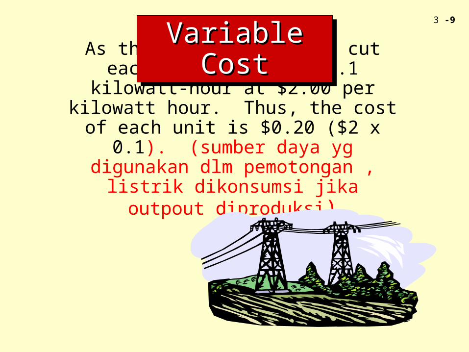
As the cutting machines cut each unit, they use 0.1 kilowatt-hour at $2.00 per kilowatt
hour. Thus, the cost of each unit is $0.20 ($2 x 0.1). (sumber daya yg digunakan dlm
pemotongan , listrik dikonsumsi jika outpout diproduksi)
Variable CostVariable CostVariable CostVariable Cost

3 -10
Total Variable Cost GraphTotal Variable Cost Graph
Cost of Power
Number of Units
$ 0 0 $ 012,000 60,000 0.2024,000 120,000 0.2036,000 180,000 0.2048,000 240,000 0.20
Units Cost
Tot
al C
osts
0Units Produced (000)
$48,000
$36,000
$24,000
$12,000
60 120 180 240
Variable CostVariable CostVariable CostVariable CostYv = .20x
3 -11
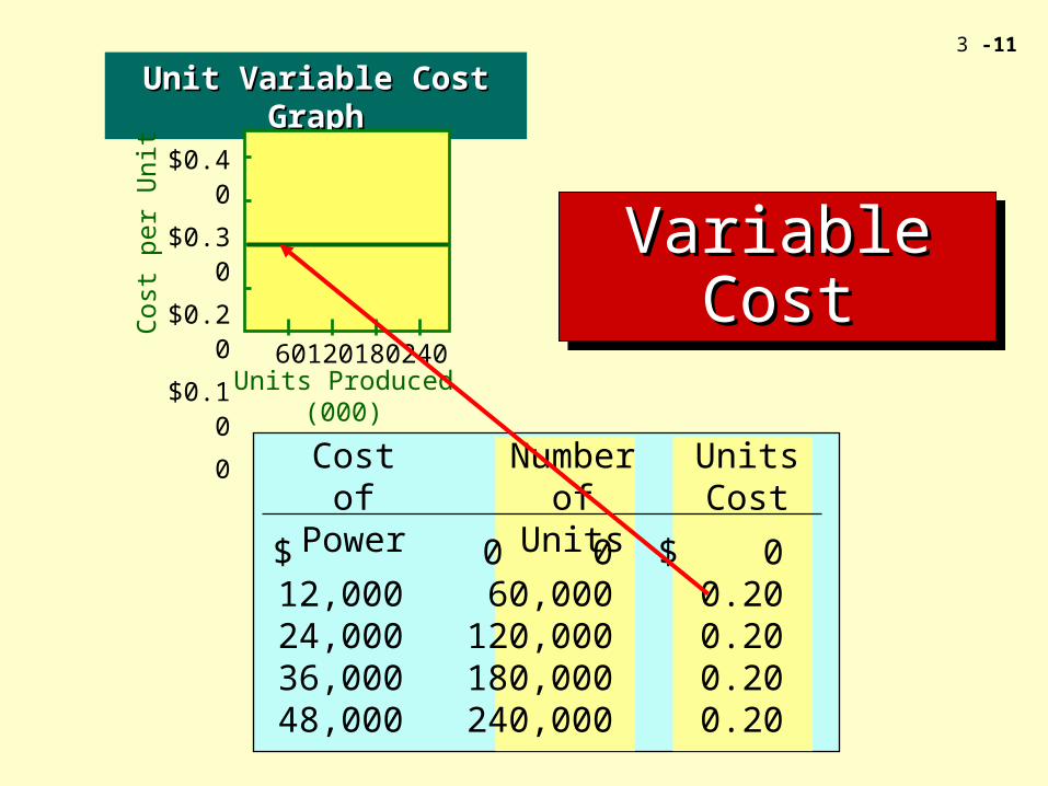
Cost of Power
Number of Units
$ 0 0 $ 012,000 60,000 0.2024,000 120,000 0.2036,000 180,000 0.2048,000 240,000 0.20
Units Cost
Variable CostVariable CostVariable CostVariable Cost
Unit Variable Cost GraphUnit Variable Cost Graph
60 120 180 240Units Produced (000)
$0.40
$0.30
$0.20
$0.10
0
Cos
t per
Uni
t
3 -12
A mixed cost is a cost that has both a fixed
and a variable component.
A mixed cost is a cost that has both a fixed
and a variable component.

3 -13
Sales representatives often are paid a
salary plus a commission on sales.
(contoh: agen penjual dibayar gaji
ditambah komisi penjualan)

3 -14
Inserts Sold
Variable Cost of Selling
40,000 $ 20,000 $30,000 $ 50,000 $1.2580,000 40,000 30,000 70,000 0.86
120,000 60,000 30,000 90,000 0.75160,000 80,000 30,000 110,000 0.69200,000 100,000 30,000 130,000 0.65
Total Selling
Cost
Fixed Cost of Selling
Selling Cost per
Unit
Mixed Cost BehaviorMixed Cost BehaviorT
otal
Cos
ts
0Units Sold (000)
$130,000$110,000$90,000$70,000$50,000
$30,000
40 80 120 160 180 200

3 -15
Activity Cost Behavior Model
Input:Input:
MaterialsMaterials
EnergyEnergy
LaborLabor
CapitalCapital
ActivitiesActivitiesActivity Activity OutputOutput
Cost BehaviorCost Behavior
Changes in Output
Changes in Input
Cost

3 -16
Flexible resources are resources acquired as used and needed. Materials and
energy are examples.
Flexible resources are resources acquired as used and needed. Materials and
energy are examples.

3 -17
Committed resources are supplied in advance of usage. Buying or leasing a building is an example of this form
of advance resource acquisition.
Committed resources are supplied in advance of usage. Buying or leasing a building is an example of this form
of advance resource acquisition.

3 -18
A step cost displays a constant level of cost for a range of output
and then jumps to a higher level of cost at some point.
A step cost displays a constant level of cost for a range of output
and then jumps to a higher level of cost at some point.
Step-Cost Behavior

3 -19
Cost
Activity Output (units)
$500
400
300
200
100
10 20 30 40 50
Step-Cost Behavior

3 -20
Normal Operating
Range) Range
(Relevant
Step-Fixed Costs
Cost
$150,000
100,000
50,000
2,500 5,000 7,500
Activity Usage
3 -21
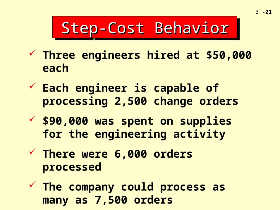
Three engineers hired at $50,000 each
Each engineer is capable of processing 2,500 change orders
$90,000 was spent on supplies for the engineering activity
There were 6,000 orders processed
The company could process as many as 7,500 orders
Step-Cost BehaviorStep-Cost BehaviorStep-Cost BehaviorStep-Cost Behavior

3 -22
Available orders = Orders used + Orders unused
7,500 orders = 6,000 orders + 1,500 orders
Fixed engineering rate = $150,000/7,500
= $20 per change order
Variable engineering rate = $90,000/6,000
= $15 per change order
Step-Cost BehaviorStep-Cost BehaviorStep-Cost BehaviorStep-Cost Behavior

3 -23
The relationship between resources supplied and resources used is expressed by the following equation:
Resources available = Resources used + Unused capacity
Step-Cost BehaviorStep-Cost BehaviorStep-Cost BehaviorStep-Cost Behavior

3 -24
Cost of orders supplied = Cost of orders used + Cost of unused orders
= [($20 + $15) x 6,000] + ($20 x 1,500)
= $240,000
Equal to the $150,000 spent on engineers and the $90,000
spent on supplies.
The $30,000 of excess engineering capacity means that a new product could be
introduced without increasing current spending on engineering.
Step-Cost BehaviorStep-Cost BehaviorStep-Cost BehaviorStep-Cost Behavior
3 -25
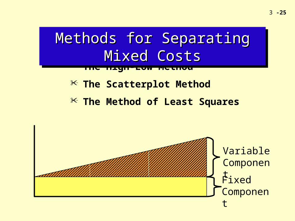
The High-Low Method
The Scatterplot Method
The Method of Least Squares
Methods for Separating Mixed CostsMethods for Separating Mixed CostsMethods for Separating Mixed CostsMethods for Separating Mixed Costs
Variable Component
Fixed Component

3 -26
The linearity assumption assumes that variable costs
increase in direct proportion to the number of units produced
(or activity units used).

3 -27
Methods for Separating Mixed CostsMethods for Separating Mixed CostsMethods for Separating Mixed CostsMethods for Separating Mixed Costs
Y = a + bx
Total Cost Total Fixed Cost
Variable Cost per
Unit
Number of Units

3 -28
Month Setup Costs Setup Hours
January $1,000 100
February 1,250 200
March 2,250 300
April 2,500 400
May 3,750 500
The High-Low MethodThe High-Low Method
Step 1: Solve for variable cost (b)Step 1: Solve for variable cost (b)

3 -29
Month Setup Costs Setup Hours
January $1,000 100
February 1,250 200
March 2,250 300
April 2,500 400
May 3,750 500
b = High Cost – Low Cost
High Units – Low Units
The High-Low MethodThe High-Low Method

3 -30
b = High Cost – Low Cost
High Units – Low Units
Month Setup Costs Setup Hours
January $1,000 100
February 1,250 200
March 2,250 300
April 2,500 400
May 3,750 500
The High-Low MethodThe High-Low Method
b = $3,750 – Low Cost
500 – Low Units

3 -31
Month Setup Costs Setup Hours
January $1,000 100
February 1,250 200
March 2,250 300
April 2,500 400
May 3,750 500
b = $3,750 – Low Cost
500 – Low Unitsb =
$3,750 – $1,000
500 – 100
The High-Low MethodThe High-Low Method

3 -32
b = $3,750 – $1,000
500 – 100
b = $6.875 b = $6.875
Step 2: Using either the high cost or low cost, solve for the total fixed cost (a).
Step 2: Using either the high cost or low cost, solve for the total fixed cost (a).
The High-Low MethodThe High-Low Method
3 -33
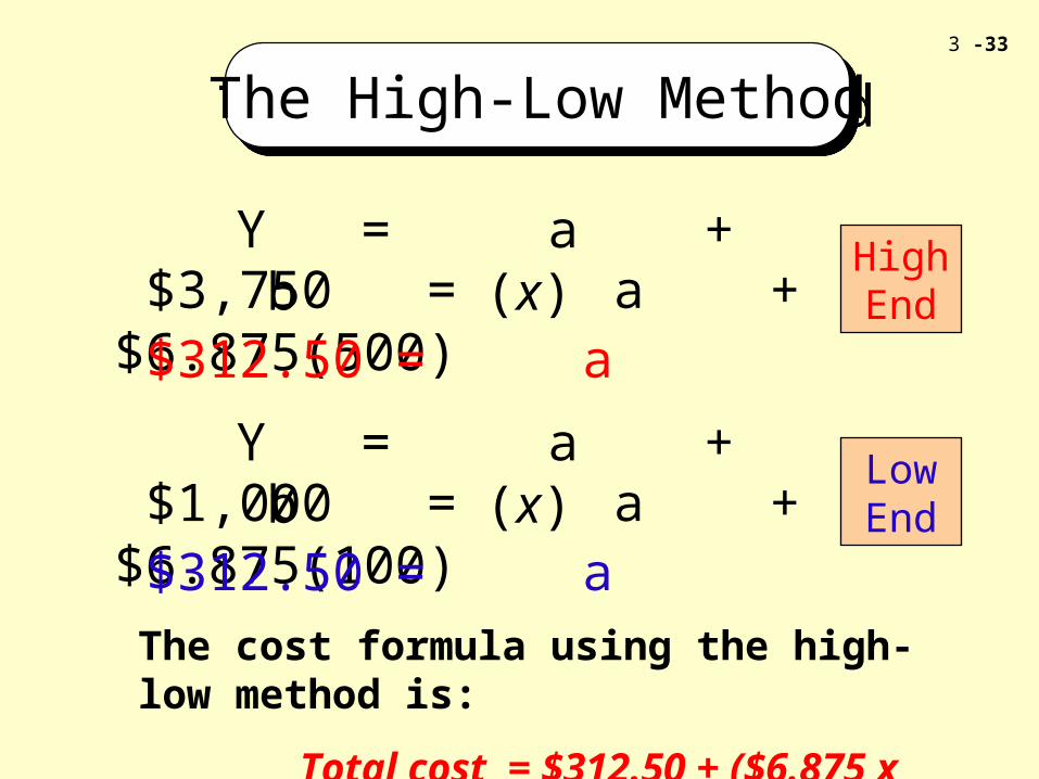
Y = a + b (x) $3,750 = a + $6.875(500) $312.50 = a
High End
Y = a + b (x) $1,000 = a + $6.875(100) $312.50 = a
Low End
The cost formula using the high-low method is:
Total cost = $312.50 + ($6.875 x Setup hours)
The High-Low MethodThe High-Low Method

3 -34
The Scatterplot MethodThe Scatterplot Method
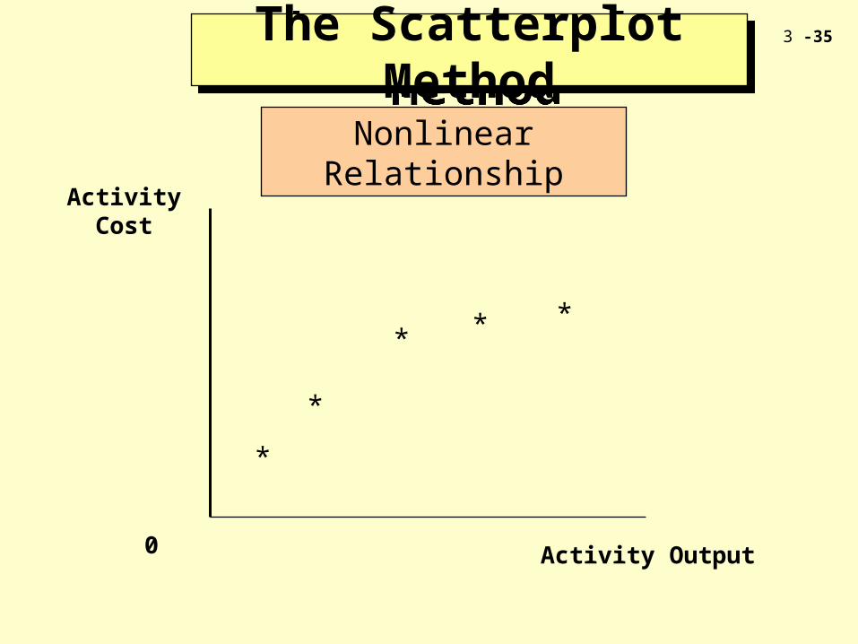
3 -35
ActivityCost
0 Activity Output
*
*
***
The Scatterplot MethodThe Scatterplot Method
Nonlinear Relationship

3 -36
ActivityCost
0 Activity Output
**
*
**
*
The Scatterplot MethodThe Scatterplot Method
Upward Shift in Cost Relationship
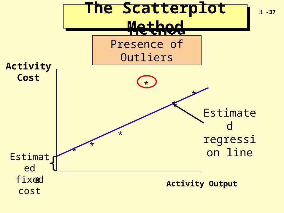
3 -37
ActivityCost
0 Activity Output
**
*
*
**
The Scatterplot MethodThe Scatterplot Method
Presence of Outliers
Estimated regression
line
Estimated fixed cost
3 -38
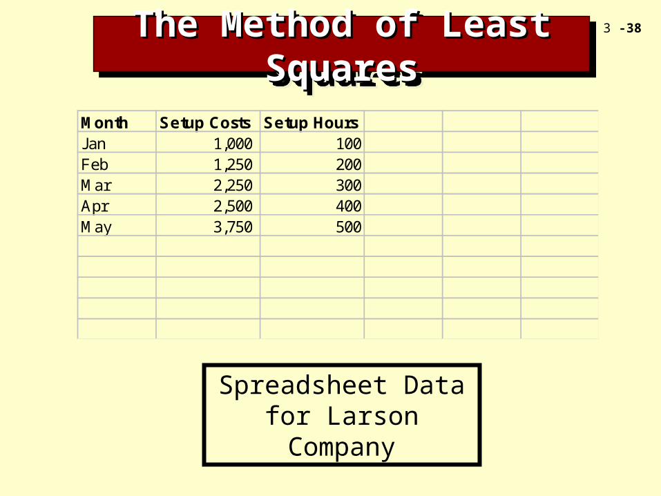
The Method of Least SquaresThe Method of Least SquaresThe Method of Least SquaresThe Method of Least Squares
Month Setup Costs Setup HoursJan 1,000 100Feb 1,250 200Mar 2,250 300Apr 2,500 400May 3,750 500
Spreadsheet Data for Larson Company

3 -39
The Method of Least SquaresThe Method of Least SquaresThe Method of Least SquaresThe Method of Least Squares
Regression Output for Larson Company
Regression Output:Constant 125Std. Err of Y Est 299.304749934466R Squared 0.944300518134715No. of Observation 5Degrees of Freedom 3X Coefficient(s) 6.75Std. Err of Coef. 0.9464847243

3 -40
The Method of Least SquaresThe Method of Least SquaresThe Method of Least SquaresThe Method of Least Squares
The results give rise to the following equation:
Setup costs = $125 + ($6.75 x Setup hours)
R2 = .944, or 94.4 percent of the variation in setup costs is explained by the number of setup hours variable.

3 -41
Coefficient of CorrelationCoefficient of Correlation
Positive Correlation
Machine Hours
Utilities Costs
r approaches +1
Machine Hours
Utilities Costs

3 -42
Coefficient of CorrelationCoefficient of Correlation
Negative Correlation
Hours of Safety
Training
Industrial Accidents
r approaches -1
Hours of Safety
Training
Industrial Accidents

3 -43
Coefficient of CorrelationCoefficient of Correlation
No Correlation
Hair Length
Accounting Grade
r ~ 0
Hair Length
Accounting Grade

3 -44
TC = b0 + ( b1X1) + (b2X2) + . . .
b0 = the fixed cost or intercept
b1 = the variable rate for the first independent variable
X1 = the first independent variable
b2 = the variable rate for the second independent variable
X2 = the second independent variable
Multiple RegressionMultiple Regression

3 -45
Multiple RegressionMultiple RegressionMonth Mhrs Summer Utilities Cost
Jan 1,340 0 $1,688Feb 1,298 0 1,636Mar 1,376 0 1,734April 1,405 0 1,770May 1,500 1 2,390June 1,432 1 2,304July 1,322 1 2,166August 1,416 1 2,284Sept 1,370 1 1,730Oct 1,580 0 1,991Nov 1,460 0 1,840Dec 1,455 0 1,833
Data for Phoenix Factory Utilities Cost Regression
3 -46
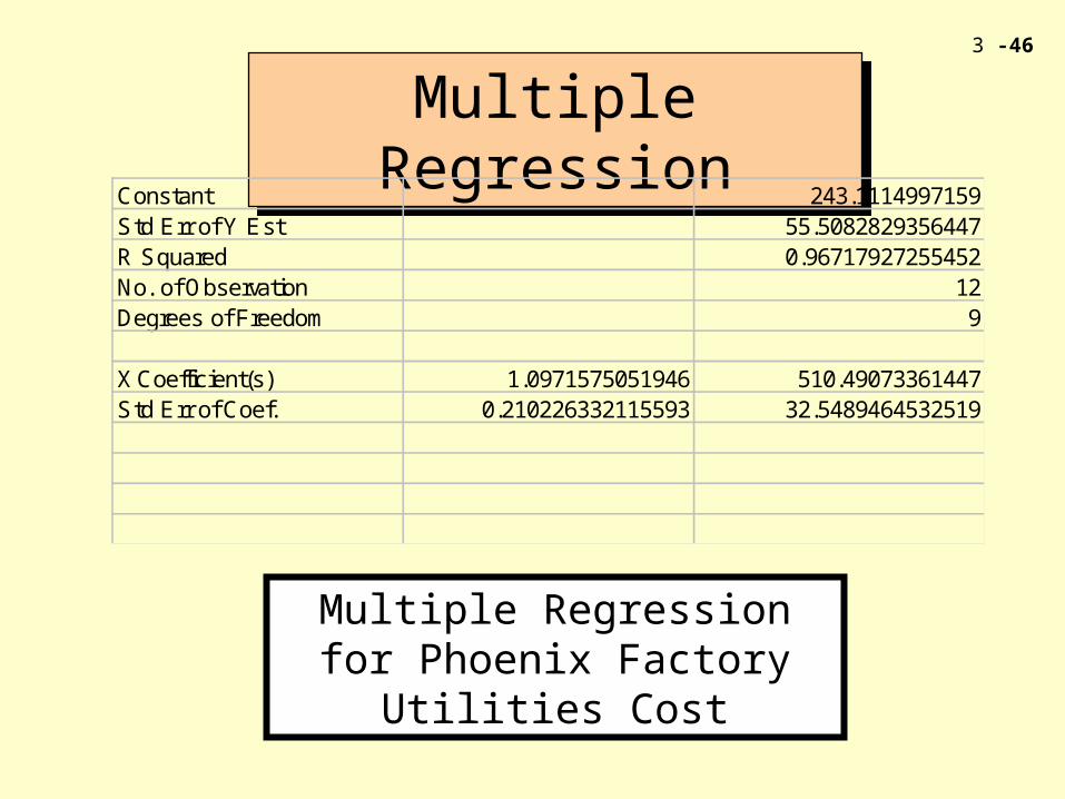
Multiple RegressionMultiple Regression
Constant 243.1114997159Std Err of Y Est 55.5082829356447R Squared 0.96717927255452No. of Observation 12Degrees of Freedom 9
X Coefficient(s) 1.0971575051946 510.49073361447Std Err of Coef. 0.210226332115593 32.5489464532519
Multiple Regression for Phoenix Factory Utilities Cost

3 -47
The results gives rise to the following equation:
Utilities cost = $243.11 + $1.097(Machine hours) + ($510.49 x Summer)
R2 = .967, or 96.7 percent of the variation in utilities cost is explained by the machine hours and summer variables.
Multiple RegressionMultiple Regression
3 -48
Managerial JudgmentManagerial JudgmentManagerial JudgmentManagerial Judgment
Managerial judgment is critically important in determining cost
behavior, and it is by far the most widely used method in practice.
Managerial judgment is critically important in determining cost
behavior, and it is by far the most widely used method in practice.
3 -49
The EndThe EndThe EndThe End
Chapter ThreeChapter Three

3 -50


![[Psy] ch03](https://img.dokumen.tips/doc/110x75/555d741ad8b42a687b8b53c6/psy-ch03.jpg)