Embed Size (px)
Citation preview

Center for Turbulence ResearchAnnual Research Briefs 2014
29
Numerical simulation of a turbulent hydraulicjump: Characterization of the free interface and
large bubble structure
By M. Mortazavi, V. Le Chenadec † AND A. Mani
1. Motivation and objectives
Bubble generation is a ubiquitous and complex phenomenon occurring as a result ofnon-linear behavior of the free surfaces. Plunging breakers, spilling breakers and plungingjets are just a few scenarios where bubble generation occurs. Due to its complexity andour lack of complete understanding of this phenomenon, the models developed in theliterature are far from being predictive (Moraga et al. 2008) (Ma et al. 2011). In additionto macro-bubble generation another mechanism has been discovered by Sigler & Mesler(1990), which generates micro bubbles, bubbles which are generated as a result of impactof two interfaces. A thin air film is trapped in a gap between the surfaces at impact.This thin film becomes unstable and fragments into tens to hundreds of micro bubbles(Thoroddsen et al. 2012). The sizes of these bubbles are in the range of tens to hundredsof microns. One important instance of bubble generation is near the ship hulls, whereturbulent boundary layer interactions with the free surface result in a large amountof macro and micro bubble entrainment. Due to their dominant buoyancy forces, largebubbles come to the interface and leave the domain much faster than micro bubbles.Micro bubbles stay under the interface for a long time and leave a trail behind the ships.Due to the complexity of this problem, we have considered a simpler case of a hydraulicjump, where turbulence interactions with a free surface generating a continuous streamof wave breaking. In this work we aim to understand the structure of the interface, thelength scales associated with them, and the local shape of the interface. Finally, we assesswhether micro-bubble generation is plausible in this scenario. Pumphrey & Elmore (1990)have characterized different bubble-generation scenarios for the case of a drop impactinga flat surface, parameterized on the drop diameter and impact velocity. Based on thisstudy, we can assess whether the impact phenomena occurring in a turbulent hydraulicjump are prone to producing micro bubbles. A hydraulic jump with a Froude numberof 2 and a Reynolds number of 11000, based on inlet height and velocity, is simulatedwith the physical density ratio of 831 after an experiment by Murzyn et al. (2005). Largebubbles are observed to form in a patch structure with the specific frequency matchingthe peak in the velocity energy spectrum.
2. Problem set up
2.1. Governing equations
The governing equations for incompressible two-phase flows include continuity and bal-ance of momentum,
∇ · u = 0
† Aerospace Engineering Department, University of Illinois at Urbana-Champaign

30 Mortazavi, Le Chenadec & Mani
∂u
∂t+ u ·∇u = −∇p
ρ+
1
ρ∇ · (µ[∇u +∇Tu ]) + g + fST ,
where u , p, ρ, µ, g and fST are velocity, pressure, density, dynamic viscosity, gravita-tional acceleration and surface tension force, respectively. Second-order accurate centraldifferencing is used on a structured uniform mesh to discretize the equations in space,and a second-order Adams-Bashforth scheme is used to discretize the equations in time.The Ghost Fluid Method is used for applying the surface tension force (Fedkiw et al.1999). In order to advect the interface a geometric Volume of Fluid (VOF) method isused (Le-Chenadec & Pitsch 2013), The equation governing the VOF reads,
∂f
∂t+ u ·∇f = 0. (2.1)
In the context of incompressible flows, the velocity divergence vanishes and we canwrite Eq. (2.1) as
Dm
Dmt
∫Ωm
fdx = 0, (2.2)
where Dm represents the material derivative and Ωm is the control volume over whichthe VOF is defined, i.e., grid cell. In addition to the VOF, a Level Set (LS) is also trackedin order to be used for accurate curvature and normal calculations,
∂G
∂t+ u ·∇G = 0.
A third-order accurate WENO scheme is used for Level Set time advection. In order tomake the two solutions of VOF and LS consistent, the level set is modified by a distancefunction constructed from the VOF field at each time step. Details of the numericalprocedures can be found in Le-Chenadec & Pitsch (2013).
2.2. Computational domain and boundary conditions
Our simulation is based on the experiment of Murzyn et al. (2005). The inflow Froudenumber, based on the inflow height and velocity, is 2. The inflow water height is h =5.9 cm and the inflow velocity is 1.5 m s−1. The Reynolds number is 11000 and theWeber number is 1866. The domain length size is chosen to be large, 20h × 4h × 4h(length× height× width), to minimize the effect of the outlet boundary condition. Wehave used a grid of 1280× 256× 256 in order to have at least three grid points across theHinze scale as reported in the experiment of Murzyn et al. (2005). Our Reynolds numberdoes not match the experiment because we have artificially increased the water viscosityfor stability reasons. Increasing the viscosity does not contaminate the results becausethe most important turbulence interaction with bubbles and interface is at the scale ofthe smallest bubbles (Hinze scale), which we capture with our grid, and turbulence atmuch smaller scales has no significant effect on bubble generation and interface dynamics.The bottom and top boundary conditions are chosen to be Neumann. Since the boundarylayer thickness does not exceed 36% of the inflow height according to the experiment, itseffect on the interface is not significant. The periodic boundary condition is used for thespanwise direction and a convective boundary condition for the outflow. At the outflowboundary, in addition to balancing the total flow rate, which is a necessary condition forthe Poisson equation (with Neumann boundary conditions for pressure) to be well-posed,we ensure that the water flow rate balances with the inflow water flow rate. Both waterand air flow rates are balanced by letting the air flow in or out at a small section of the

Numerical simulation of a turbulent hydraulic jump 31
(a) (b)
Figure 1. Two regions in a hydraulic jump with different bubble generation mechanisms andvoid fraction characteristics.(a) Lower region of the jump (turbulent shear region). (b) Upperregion of the jump (roll-up region).
outflow boundary. This treatment does not affect the flow inside the domain nor does itaffect the stability of the code. The inflow boundary condition is uniform for the waterand is a sharp 1D Blasius divergence-free velocity profile for the air side.
3. Validation
3.1. Bubble generation
There are two regions of bubble generation with different characteristics, as argued byMurzyn et al. (2005). Figure 1 shows these two regions. The lower region, Figure 1(a),is characterized by an advection-diffusion process, and the interaction of the interfaceis minimal in this region. Therefore, the bubbles generated at the toe are convectedand diffused downstream of the flow. According to Chanson (1996), the void fractionin this region can be expressed as a Gaussian profile, which is the solution to a steadyadvection-diffusion process,
C = Cmax exp
[−1
4
U
D
(z − zCmax)2
x
], (3.1)
where x, Cmax, U , D and zCmax are, respectively, stream-wise location, maximum voidfraction, characteristic velocity, effective diffusivity and vertical location of the maximumvoid fraction, all at the particular x location. Murzyn et al. (2005) also showed that theirresults follow a Gaussian profile with appropriate coefficients, which they report in theexperiment.
We compare our time and span-wise averaged void fraction, C, to the experiment, as
a function of the similarity variable (U/4xD)1/2
(z − zCmax) in Figure 2. The simulationresults agree with the experiment very well, and we can see the self-similar behavior ofthe void fraction in the lower region of the hydraulic jump.
The upper region is a result of interfacial aeration as argued by Murzyn et al. (2005),and a good fit to the void fraction is found by Brattberg et al. (1998), and is in the formof an error function (Eq. (3.2)),
C =1
2erf
(z − zC50
2√Dx/U
), (3.2)

32 Mortazavi, Le Chenadec & Mani
0 0.5 1 1.5−5
−4
−3
−2
−1
0
1
2
C/Cmax
(U/4
xD
)1/2
(z−
zC
max)
Gaussian Profile
x=0.85
x=1.70
x=2.54
Figure 2. Simulation results of void fraction in the lower region of a hydraulic jump for differentstream-wise locations compared with the theoretical and experimentally validated Gaussianprofile (Murzyn et al. 2005).
0 0.2 0.4 0.6 0.8 1−6
−4
−2
0
2
4
C
1/2
(Dx/U
)−1/2
(z−
zC
50)
Error function
x=1.70
x=2.54
x=4.24
Figure 3. Simulation results of void fraction in the upper region of a hydraulic jump for differentstream-wise locations compared with the experimentally suggested error function of Eq (3.2),(Murzyn et al. 2005).
where zC50 is the vertical position for which the void fraction equals one half. The voidfraction is not normalized in this case since the maximum value is one in the air side.
Similarly, by using the values for the zC50 and D/Uh from the experiment, we comparethe simulation results with the suggested fit in Eq. (3.2) in Figure 3. The value of zC50
used for the plot comes from the simulation itself. We notice a discrepancy of at most30% between the value of zC50 in the simulation and experiment, which may be due
Numerical simulation of a turbulent hydraulic jump 33
100
101
10−1
100
101
(x−xt)/h
L/h
Fr=2.0 Murzyn 2007
Fr=2.4 Murzyn 2007
Fr=3.7 Murzyn 2007
Fr=4.8 Murzyn 2007
Exp Fit
Simulation
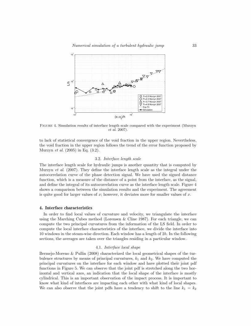
Figure 4. Simulation results of interface length scale compared with the experiment (Murzynet al. 2007).
to lack of statistical convergence of the void fraction in the upper region. Nevertheless,the void fraction in the upper region follows the trend of the error function proposed byMurzyn et al. (2005) in Eq. (3.2).
3.2. Interface length scale
The interface length scale for hydraulic jumps is another quantity that is computed byMurzyn et al. (2007). They define the interface length scale as the integral under theautocorrelation curve of the phase detection signal. We have used the signed distancefunction, which is a measure of the distance of a point from the interface, as the signal,and define the integral of its autocorrelation curve as the interface length scale. Figure 4shows a comparison between the simulation results and the experiment. The agreementis quite good for larger values of x; however, it deviates more for smaller values of x.
4. Interface characteristics
In order to find local values of curvature and velocity, we triangulate the interfaceusing the Marching Cubes method (Lorensen & Cline 1987). For each triangle, we cancompute the two principal curvatures from the information of the LS field. In order tocompute the local interface characteristics of the interface, we divide the interface into10 windows in the steam-wise direction. Each window has a length of 2h. In the followingsections, the averages are taken over the triangles residing in a particular window.
4.1. Interface local shape
Bermejo-Moreno & Pullin (2008) characterized the local geometrical shapes of the tur-bulence structures by means of principal curvatures, k1 and k2. We have computed theprincipal curvatures on the interface for each window and have plotted their joint pdffunctions in Figure 5. We can observe that the joint pdf is stretched along the two hor-izontal and vertical axes, an indication that the local shape of the interface is mostlycylindrical. This is an important observation of the impact process. It is important toknow what kind of interfaces are impacting each other with what kind of local shapes.We can also observe that the joint pdfs have a tendency to shift to the line k1 = k2

34 Mortazavi, Le Chenadec & Mani
−20 0 20
−30
−20
−10
0
10
20
30
K1
K2
Window 3
−20 0 20 40
−30
−20
−10
0
10
20
30
K1
K2
Window 4
−20 0 20 40
−30
−20
−10
0
10
20
30
K1
K2
Window 5
−20 0 20 40
−30
−20
−10
0
10
20
30
K1
K2
Window 6
−20 0 20 40
−30
−20
−10
0
10
20
30
K1
K2
Window 7
−20 0 20 40
−30
−20
−10
0
10
20
30
K1
K2
Window 8
Figure 5. First principal curvature vs. second principal curvature on the interface for differentstream-wise locations of the hydraulic jump. Each window has a length of 2h. Window 3 startsat the toe of the jump.
for larger values of x (larger window numbers). The reason is that the area ratio of thebubbles to total area increases for those places as compared to the windows closer tothe toe of the jump. Since the line of k1 = k2 is a characteristic of a spherical shapeand indicates the presence of the bubbles, the contours shift towards this line for largerwindow numbers.
4.2. Interface curvedness distribution
Interface curvedness, as apparent by its name, is a measure of how much an interface iscurved (Bermejo-Moreno & Pullin 2008). It also reduces the two principal curvatures toa single number, making it a convenient way to measure the local interface curvature. Itis defined as the geometrical mean of the two principle curvatures,
Numerical simulation of a turbulent hydraulic jump 35
C =
√κ2
1 + κ22
2.
To gain insight into the curvedness distribution along the interface of the turbulent hy-draulic jump, we have computed the Probability Density Function (PDF) of the curved-ness for different positions of the jump. Figure 6 shows the PDF of the curvedness on theinterface. The PDF of the curvedness is computed based on area. The sum of the areaof a particular curvedness divided by the total area is a measure of probability of findinga point with that particular curvedness on the interface. The results for two differentresolutions are shown in Figure 6. The solid line represents the grid of 1280× 256× 256and the dash-dotted line represents a mesh with half the resolution in each direction.The finer mesh resolves smaller structures, the reason why the value of the PDF for thefine mesh at larger values of curvedness is higher. The vertical dashed lines represent thevalues of curvedness for which the calculations of curvedness for coarse and fine grids areunreliable. The values for the maximum curvedness, according to our assessments on acanonical case of a sphere, are set to 1.5/∆x. Interestingly, we can observe a power lawdistribution for the PDFs with the slope of −5/3 which extends for a long range.
4.3. Potential interface impact and micro-bubble generation
Pumphrey & Elmore (1990) have studied different types of bubble generation for thecase of a droplet impacting a flat surface of the same liquid. They have organized theirobservations into a plot, which is shown in Figure 7. Droplet diameter and impact ve-locity are the parameters which determine the type of bubble generation. Micro-bubblegeneration is observed to occur for relatively low velocities. In this study, in Figure 8,we have plotted the joint PDF of the velocity fluctuations from the mean value at theinterface and the equivalent diameter corresponding to the interface. Since we know thatthe local shape of the interface is mostly cylindrical, the local equivalent diameter canbe defined based on the curvedness as D =
√2/C. The joint PDF shows that if impact
happens on the interface, based on the relative velocity of the two impacting interfaces(characterized by the velocity fluctuations) and their shape (characterized by the equiv-alent diameter), there is a strong likelihood that micro-bubble generation occurs, in thedomain. Experimental observations of micro-bubble generation are also plotted on topof simulation results in Figure 8.
5. Large bubble formation structure
5.1. Velocity energy spectrum and connection with bubble generation
The energy spectra of the three components of velocity are computed as a functionof frequency for three locations of the jump, x/h = 6, 8, 10, shown in Figures 9-11.We averaged the spectra in the periodic span-wise direction. Two grid resolutions arecompared. The fine grid of 1280 × 256 × 256 is compared with the results of the coarsegrid, which has half the grid resolution in each direction. The slope of −5/3 is observedin the inertial range of the turbulence spectrum. Liu et al. (2004) have also reportedon the spectrum of their hydraulic jump experiments, and they have also observed the−5/3 slope. Note that the Kolmogorov energy cascade assumption to smaller scales isalso valid for highly bubbly two-phase flows.
Another interesting observation from the energy spectrum profiles is that a distinctivefrequency is recognizable, especially for the vertical velocity component, which is believed

36 Mortazavi, Le Chenadec & Mani
100
101
10−6
10−5
10−4
10−3
10−2
10−1
100
Curvedness
PD
F
Window 3
100
101
10−6
10−5
10−4
10−3
10−2
10−1
100
Curvedness
PD
F
Window 4
100
101
10−6
10−5
10−4
10−3
10−2
10−1
100
Curvedness
PD
F
Window 5
100
101
10−6
10−5
10−4
10−3
10−2
10−1
100
Curvedness
PD
F
Window 6
100
101
10−6
10−5
10−4
10−3
10−2
10−1
100
Curvedness
PD
F
Window 7
100
101
10−6
10−5
10−4
10−3
10−2
10−1
100
Curvedness
PD
F
Window 8
Figure 6. Interface curvedness PDF for different locations of the jump. Each window has alength of 2h and window 3 starts at the toe of the jump. Solid line: fine grid, dash-dotted line:coarse grid, dotted line: slope of −5/3, and vertical dashed line: values of curvedness after whichthe simulation results are not reliable (computed as 1.5/∆x).
to be the result of the bubble-generation mechanism and the structure of the flow. Thesepeaks are at frequencies of 3.47Hz and 3.97Hz for locations x/h = 8 and x/h = 10,respectively, which correspond to non-dimensional Srtouhal numbers of S = fh/U1 =0.136 and S = fh/U1 = 0.156.
5.2. Large bubble-patch structure
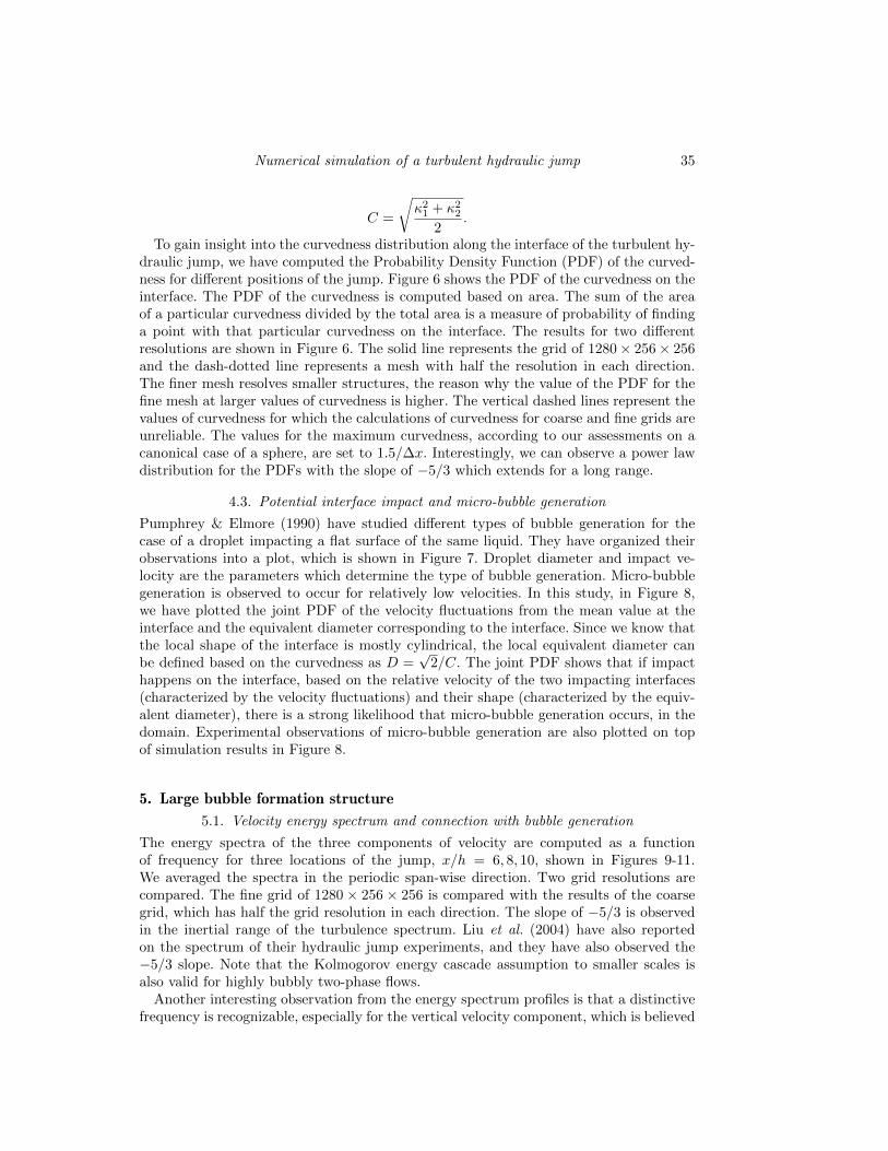
Visual observations of bubble generation suggest that the large bubbles are generated ina patch-structure pattern and are generated periodically (Figure 12). Therefore, there is

Numerical simulation of a turbulent hydraulic jump 37
Figure 7. Pumphrey diagram of bubble generation for droplet impact on a flat surface of thesame liquid, Pumphrey & Elmore (1990).
0 1 2 3 4 5 6 70
0.5
1
1.5
2
2.5
3
3.5
4
4.5
5
D (mm)
|V−
Vm
| (m
/s)
Window 5
Esmailizadeh, MeslerSigler, Mesler
Mills, SaylorThoroddsen et. al.
Figure 8. Joint PDF of velocity fluctuations on the interface and interface equivalentdiameter computed from the curvedness D =
√2/C.
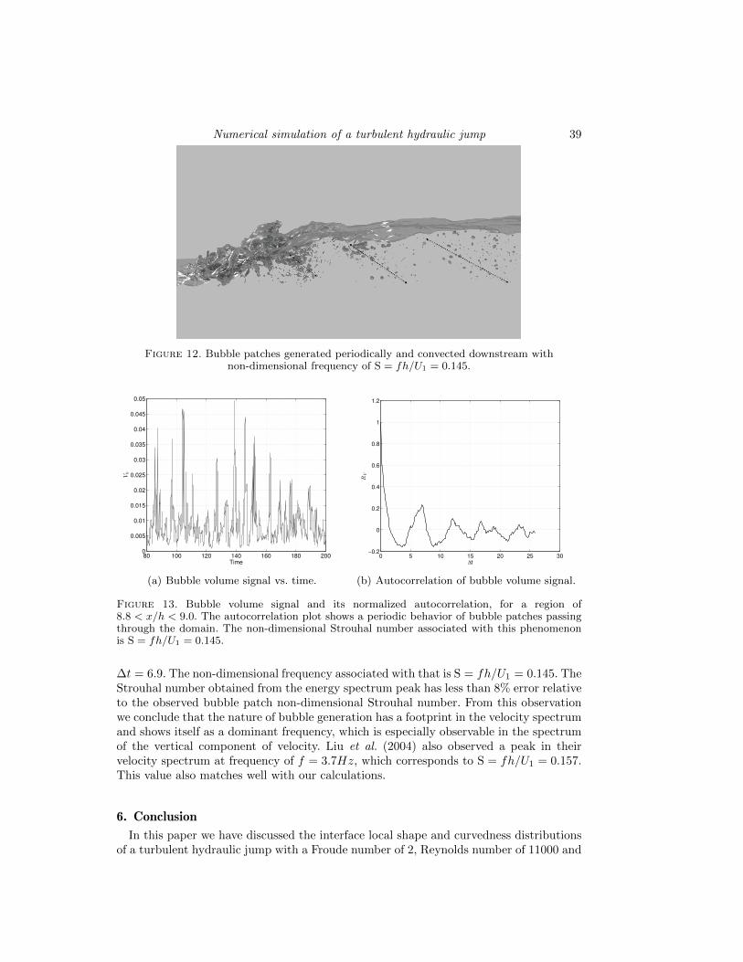
an intrinsic frequency associated with this bubble-patch generation. In order to quantifythis frequency we have divided the domain into 100 sections and computed the voidfraction in each section as a function of time. Figure 13(a) shows this void fraction signalfor the interval of 8.8 < x/h < 9.0 . This interval was chosen because it is neither tooclose to the jump toe, where the bubble patches are still not fully formed, not too far fromit, where the bubbles are too dissipated and the void fraction signal becomes faded andthe frequency is not recognizable. Figure 13(b) shows the autocorrelation of the signalas computed from Eq. (5.1).
RV (∆t) =
∫ T
0Vb(t)Vb(t+ ∆t)dt∫ T
0Vb(t)Vb(t)dt
. (5.1)

38 Mortazavi, Le Chenadec & Mani
100
102
10−6
10−5
10−4
10−3
10−2
Frequency (Hz)
−5/3
Fine
Coarse
(a) u spectrum
101
102
10−6
10−5
10−4
10−3
10−2
Frequency (Hz)
−5/3
Fine
Coarse
(b) v spectrum
Figure 9. Energy spectrum of velocity components for x/h = 6.
100
102
10−6
10−5
10−4
10−3
10−2
Frequency (Hz)
−5/3
Fine
Coarse
(a) u spectrum
100
102
10−6
10−5
10−4
10−3
10−2
Frequency (Hz)
−5/3
Fine
Coarse
(b) v spectrum
Figure 10. Energy spectrum of velocity components for x/h = 8.
100
102
10−6
10−4
10−2
Frequency (Hz)
−5/3
Fine
Coarse
(a) u spectrum
100
102
10−6
10−5
10−4
10−3
10−2
Frequency (Hz)
−5/3
Fine
Coarse
(b) v spectrum
Figure 11. Energy spectrum of velocity components for x/h = 10.
The autocorrelation plot shows the periodic behavior of the void fraction signal. Theperiod can be determined from the first peak of the plot, which occurs for non-dimensional
Numerical simulation of a turbulent hydraulic jump 39
Figure 12. Bubble patches generated periodically and convected downstream withnon-dimensional frequency of S = fh/U1 = 0.145.
80 100 120 140 160 180 2000
0.005
0.01
0.015
0.02
0.025
0.03
0.035
0.04
0.045
0.05
Time
Vb
(a) Bubble volume signal vs. time.
0 5 10 15 20 25 30−0.2
0
0.2
0.4
0.6
0.8
1
1.2
∆t
RV
(b) Autocorrelation of bubble volume signal.
Figure 13. Bubble volume signal and its normalized autocorrelation, for a region of8.8 < x/h < 9.0. The autocorrelation plot shows a periodic behavior of bubble patches passingthrough the domain. The non-dimensional Strouhal number associated with this phenomenonis S = fh/U1 = 0.145.
∆t = 6.9. The non-dimensional frequency associated with that is S = fh/U1 = 0.145. TheStrouhal number obtained from the energy spectrum peak has less than 8% error relativeto the observed bubble patch non-dimensional Strouhal number. From this observationwe conclude that the nature of bubble generation has a footprint in the velocity spectrumand shows itself as a dominant frequency, which is especially observable in the spectrumof the vertical component of velocity. Liu et al. (2004) also observed a peak in theirvelocity spectrum at frequency of f = 3.7Hz, which corresponds to S = fh/U1 = 0.157.This value also matches well with our calculations.
6. Conclusion
In this paper we have discussed the interface local shape and curvedness distributionsof a turbulent hydraulic jump with a Froude number of 2, Reynolds number of 11000 and

40 Mortazavi, Le Chenadec & Mani
Weber number of 1866, following the experiment of Murzyn et al. (2005). We comparedthe void fraction and interface length scale with the experimental results, which showedgood agreement between them. We have observed that the impact events on the interfacehave a strong likelihood of generating micro bubbles based on the experimental obser-vations of Pumphrey & Elmore (1990). Velocity energy spectra for different stream-wiselocations of the hydraulic jump were computed. A −5/3 power law is observed in theinertial range and the presence of a dominant peak is noticed. This dominant frequencyis associated with the bubble-generation mechanism. The frequency of the peak matcheswith the frequency of the bubble-patch generation.
REFERENCES
Bermejo-Moreno, I. & Pullin, D. I. 2008 On the non-local geometry of turbulence.J. Fluid Mech. 603, 101–135.
Brattberg, T., Toombes, L. & Chanson, H. 1998 Developing air-water shear lay-ers of two-dimensional water jets discharging into air. ASME Fluids EngineeringDivision Summer Meeting .
Chanson, H. 1996 Air Bubble Entrainment in Free Surface Turbulent Flows. AcademicPress.
Fedkiw, R., Aslam, T., Merriman, B. & Osher, S. 1999 A non-oscillatory eulerianapproach to interfaces in multi material flows (the ghost fluid method). J. Comput.Phys 152, 457–492.
Le-Chenadec, V. & Pitsch, H. 2013 A 3d unsplit forward/backward volume-of-fluidapproach and coupling to the level set method. J. Comput. Phys 233, 10–33.
Liu, M., Rajaratnam, N. & Zhu, D. Z. 2004 Turbulence structure of hydraulic jumpsof low froude numbers. J. Hydraul. Eng. 130, 511–520.
Lorensen, W. E. & Cline, H. E. 1987 Marching cubes: a high resolution 3d surfacecontraction algorithm. ACM SIGGRAPH Computer Graphics 21, 163–169.
Ma, J., Oberai, A. A., Jr, R. T. L. & Drew, D. A. 2011 Modeling air entrainmentand transport in a hydraulic jump using two-fluid rans and des turbulence models.Heat Mass Transfer. 47, 911–919.
Moraga, F., Carrica, P., Drew, D. & Jr, R. L. 2008 A sub-grid air entrainmentmodel for breaking bow waves and naval surface ships. Comput. & Fluids 37, 281–298.
Murzyn, F., Mouaze, D. & Chaplin, J. 2005 Optical fibre probe measurements ofbubbly flow in hydraulic jumps. Int. J. Multiphase Flow 31, 141–154.
Murzyn, F., Mouaze, D. & Chaplin, J. 2007 Air-water interface dynamic and freesurface features in hydraulic jumps. J. Hydraul. Res. 45, 679–685.
Pumphrey, H. C. & Elmore, P. A. 1990 The entrainment of bubbles by drop impacts.J. Fluid Mech. 220, 539–567.
Sigler, J. & Mesler, R. 1990 The behavior of the gas film formed upon drop impactwith a liquid surface. J. Colloid Interf. Sci. 134, 459–474.
Thoroddsen, S., Thoraval, M., Takehara, K. & Etoh, T. 2012 Micro-bubblemorphologies following drop impacts onto a pool surface. J. Fluid Mech. 708, 469–479.