National Environmental Research InstituteMinistry of the Environment . Denmark

Carbon dioxide exchange in the High Arctic – examples from terrestrial ecosystemsPhD thesis, 2006

Louise Grøndahl

[Blank page]

National Environmental Research InstituteMinistry of the Environment . Denmark

Carbon dioxide exchange in the High Arctic – examples from terrestrial ecosystemsPhD thesis, 2006

Louise Grøndahl

PhD project carried out in collaboration between:National Environmental Research InstituteInstitute of Geography, University of Copenhagen

Data sheet Title: Carbon dioxide exchange in the High Arctic - examples from terrestrial ecosystems Subtitle: PhD thesis 2006

Author: Louise Grøndahl Department: Department of Arctic Environment University: University of Copenhagen, Institute of Geography

Publisher: National Environmental Research Institute ©Ministry of the Environment

URL: http://www.dmu.dk

Year of publication: December 2006

Public defence: September 2006 by Dr. Richard Harding, Centre for Ecology and Hydrology, Wallingford, United Kingdom; Associate professor, PhD Eva Bøgh, Department of Geography and Interna-tional Development Studies, University of Roskilde; Associate professor, PhD Helge Ro-Poulsen, Institute of Biology, University of Copenhagen

Supervisors: Associate Professor, PhD Thomas Friborg, Institute of Geography; Research Scientist, PhD Mikkel P. Tamstorf, Department of Arctic Environment, National Environmental Research Insti-tute

Financial support: COGCI, Copenhagen Global Change Initiative, University of Copenhagen and National Envi-ronmental Research Institute

Please cite as: Grøndahl, L. 2006: Carbon dioxide exchange in the High Arctic – examples from terrestrial ecosystems. PhD thesis. Dept. of Arctic Environmental, NERI and Institute of Geography, Uni-versity of Copenhagen. National Environmental Research Institute, Roskilde, Denmark. 210 pp. http://www.dmu.dk/Pub/PHD_LGR.pdf

Reproduction is permitted, provided the source is explicitly acknowledged.

Abstract: The thesis provides an analysis of the exchange of CO2 between the atmosphere and the vegeta-tion communities in the High Arctic at different temporal and spatial scales. Using a time series of data from a dry heath ecosystem in Zackenberg NE Greenland, it was shown that timing of snowmelt and temperature in the growing season strongly control the interannual variability in ecosystem CO2 uptake rates. The area has during the past years experienced a warming during the summer season, which was shown to increase the uptake of CO2 by the vegetation. The in-creasing earlier snowmelt prolonged the length of the growing season, which in combination with high temperatures increased uptake rates. The dry heath ecosystem in general gained car-bon during the summer season in the order of magnitude -1.4 gCm-2 up to 32 gCm-2. This result is filling out a gap of knowledge on the response of high Arctic ecosystems to increased warm-ing in the region. A cross scale analysis of eddy covariance and chamber data showed a good agreement between the two methods, which lead to an estimate of CO2 exchange based on NDVI. A timeseries of satellite imagery for the 2004 growing season provided the opportunity to upscale fluxes from the measurements conducted in the valley to a regional level. Including information on temporal and spatial variability in air temperature and radiation, together with NDVI and a vegetation map a regional estimate of the CO2 exchange during the summer was provided, elaborating the NDVI based estimate on net carbon exchange.

Keywords: Carbon dioxide, High Arctic ecosystems, upscaling, satellite remote sensing

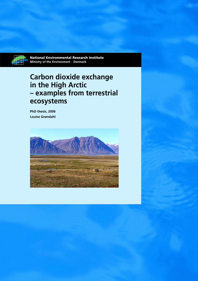
Layout: Louise Grøndahl Photo frontpage: Louise Grøndahl

Paper quality: Cyclus Offset Printed by: Schultz Grafisk

Environmental certified (ISO 14001) and Quality certified (ISO 9002)

ISBN: 978-87-7772-961-4 Number of pages: 210

Internet-version: The report is available electronic format (pdf) at NERI’s website http://www.dmu.dk/Pub/PHD_LGR.pdf

For sale at: Ministry of the Environment Frontlinien Rentemestervej 8 DK-2400 Copenhagen NV Denmark Tel. +45 70 12 02 11 frontlinien@frontlinien.dk

Table of contents

Preface 2

List of publications included in the thesis 4

Abstract 5

Sammenfatning 6

1 Introduction 8

Objectives 10

2 Background for the thesis work 11

2.1 The Arctic Region 11

2.2 Zackenberg Research Area 12

2.2.1 Vegetation in the Zackenberg area 14

2.3 CO2 exchange in the Arctic 15

2.4 Carbon cycling in the Arctic 16

2.5 Methods of assessing the CO2 exchange 19

2.6 Application of remote sensing for estimating regional budgets 22

3 Results and discussion 24

3.1 Seasonality in Net Ecosystem Exchange in the Arctic 24

3.2 Interannual variation 27

3.3 Comparison of methods 29

3.4 Fluxes from different vegetation types 30

3.5 Upscaling the CO2 fluxes 31

3.6 Changes in circumpolar CO2 flux 33

4 Concluding remarks and perspectives 34

5 References 36

2

Preface

The current thesis is submitted to the Faculty of Science, University of Copenhagen

for the fulfilment of a PhD degree. During the thesis work I was based at National

Environmental Research Institute, Department of Arctic Environment and registered

at the COGCI (Copenhagen Global Change Initiative) Ph.D. School. Field work in

NE Greenland was feasible through the funding for the project Spectral Calibration of

High Arctic Primary Production Estimation (SCHAPPE). The project was financially

supported by the Danish Ministry of Environment (Dancea), the Aage V. Jensens

Foundation and the Danish Research Council. Without the unique ZERO (Zackenberg

Ecological Research Operations) monitoring programmes in Zackenberg, this work

would not have been possible. My sincere thanks to the people behind the

programmes. The Danish Polar Center is acknowledged for providing excellent

logistical support during the field work.

During the years of this thesis work I was lucky to be surrounded by very helpful

colleagues at the National Environmental Research Institute (NERI). I would like to

express thanks to my colleagues (too many to mention you all) at NERI for answering

questions and keeping an open door for me, it has been a pleasure working with you

all. Especially I would express thanks to Hans Meltofte for sharing his knowledge

achieved from many years in the Arctic. Also David Boertmann and Peter Aastrup are

thanked for valuable information on the High Arctic and comments on the work along

the way. I would also like to acknowledge my supervisor, Thomas Friborg, Institute

of Geography, University of Copenhagen (IGUC) for sharing knowledge on fluxes,

reading manuscripts and general discussions on the project and co-supervisor Mikkel

P. Tamstorf, NERI for reading manuscripts and discussing various parts of the

project.

At the Institute of Geography, University of Copenhagen (IGUC) I have also had

some good colleagues. I am indebted to Charlotte Sigsgaard for always being ready to

answer questions on what ever I could come to ask for and sharing her office with me

during my weekly work-hours at the IGUC. Thanks also goes to the people I have

been working with over the past years, especially Henrik Søgaard for introducing me

to this exciting area of gas-fluxes many years ago and always having interest in the

3

current work and Birger U. Hansen for kind help along the process. Also the people at

the Institute of Terrestrial Ecology Lotte Illeris and Anders Michelsen for interesting

discussions on the data. Torben R. Christensen University of Lund for answering

questions with great enthusiasm.

Thanks go to my family and friends for their support and help during the work,

especially my husband Martin for “taking-care-of-business” while I was working.

And finally Josefine and Magnus for constantly reminding me what’s important in life

and being such happy and harmonic children.

Louise Grøndahl

Copenhagen, June 2006

4

List of publications included in the thesis

The thesis consists of a synopsis and five scientific papers which present the results of

the work conducted during the PhD study on carbon dioxide exchange in a High

Arctic ecosystem. The synopsis gives the background of this work.

Paper I: Grøndahl, L, Friborg, T. and Soegaard, H. Temperature and snowmelt

controls on the carbon exchange in a high arctic ecosystem. In Press Theoretical and

Applied Climatology

Paper II: Grøndahl, L. Tamstorf, M., Friborg, T., Soegaard, H., Illeris, L., Hansen B.

U., Albert, K., Arndal, M., Pedersen, M.R. and Michelsen, A. Scaling CO2 fluxes

from plot- and field-level to landscape-level in a high arctic ecosystem using a

footprint model and satellite images. Submitted Global Change Biology

Paper III: Grøndahl, L., Friborg, T., Tamstorf, M., Sigsgaard, C, Hansen, B.U.,

Illeris, L. and Michelsen, A.. Assessing a regional carbon dioxide budget for the

growing season of a High Arctic area. Submitted Tellus Series B – Chemical and

Physical Meteorology Special Issue

Paper IV: Soegaard, H., Sørensen, L., Rysgaard, S., Grøndahl, L., Elberling, B.,

Friborg, T. S.E. Larsen and J. Bendtsen (2004). High Arctic Carbon Sink

Identification – A System Approach. IGBP NewsLetter No. 59, p. 11-14

Paper V: Christensen, T.R., C. E. Tweedie, T. Friborg, M. Johansson, P. M. Crill, J.

A. Gamon, L. Groendahl, J. Gudmundsson, Y. Harazono, C. Lloyd, P. J. Martikainen,

W.C. Oechel, H. Oskarsson, N. Panikov and P.A. Wookey. Carbon fluxes and their

controlling processes in Arctic tundra: Current knowledge and challenges. Submitted

Ecological Applications

5

AbstractThis thesis is a study of the CO2 exchange between a High Arctic tundra site and the

atmosphere. The thesis focuses on an analysis of the monitoring data obtained in the

Zackenberg research area, NE Greenland. Continuous summer-time Net Ecosystem

CO2 Exchange measurements have been conducted by Zackenberg Ecological

Research Operations (ZERO) research program at a dry dwarf shrub heath since 2000.

The measurements from the eddy covariance (EC) mast provide a unique series of

measurements on CO2 exchange from a High Arctic locality. This thesis work

presents the fluxes from this monitoring.

During the years of monitoring in Zackenberg, the dry ecosystem has been net

sequestering CO2. This is mainly attributed to two abiotic factors; air temperature and

timing of snow-melt. The summer-time temperature and the increasingly early snow-

melt in the area and a limited increase in air temperature during the growing season

increased uptake rates for the ecosystem. A high degree of interannual variability in

the carbon gained during the growing season was seen. The interannual variability

seems best explained through differences in the length of the growing season and the

amount and rate of snow-melt. The annual status of this High Arctic tundra site is

however still unknown, due to the lack of measurements from the highly important

autumn and winter period.

Additionally measurements were undertaken at five different dominating vegetation

types in the area using the chamber technique. Within the different vegetation types a

high degree of spatial and temporal variability is seen within the growing season. The

variability in flux might partly be related to the difference in vegetation composition

in the plots. The CO2 exchange obtained from the chamber measurements were

compared to the EC measurements from a dry site using a footprint model. An overall

agreement was found between the two methods, which allows an upscaling attempt.

Upscaling were attempted using two approaches. Based on a vegetation map and a

simple model the Net Ecosystem Exchange was derived and additionally the flux

assignments approach was tried. It was found that the region is a net consumer of CO2

during the growing season.

6

Sammenfatning Gennem tiderne har klimaet i det arktiske område varieret. I det seneste århundrede er

der sket en forøget opvarmning i området, hvilket forventes at fortsætte i dette

århundrede. Opvarmningen forventes at have effekt på økosystemerne i regionen. Det

er derfor afgørende at have kendskab til hvordan økosystemerne reagerer på abiotiske

faktorer i det nuværende klima, for at være i stand til at forudsige hvordan ændringer i

klimaet fremover vil påvirke området. Udvekslingen af drivhus gassen kuldioxid

(CO2) er en af de faktorer der fremover kan have indflydelse på klimaudviklingen i

Arktis, idet disse områder indeholder store mængder kulstof opmagasineret i jorden.

Udvekslingen af CO2 mellem økosystemerne og atmosfæren er kun undersøgt i få

arktiske områder og oftest kun som sporadiske målinger foretaget få gange i løbet af

sommer sæsonen, hvilket betyder at yderligere undersøgelser er vigtige. I Zackenberg,

NØ Grønland er et måleprogram igangsat med det formål at monitere fysiske og

biologiske parametres respons på klimaændringerne.

Dette PhD projekt omhandler udvekslingen af CO2 mellem en høj arktisk tundra i

Zackenberg og atmosfæren. Projektet er et resultat af bearbejdningen af eddy

covarians (EC) moniterings data fra en tør hede samt af målinger med kamre i fem

dominerende vegetations typer i samme område. Projektet fokuserer på at beskrive de

abiotiske faktorer der kan forklare den målte CO2 udveksling i sommer sæsonen på

denne høj arktiske lokalitet. På baggrund af undersøgelserne i dette projekt kan det på

baggrund af de seneste 7 års EC målinger konkluderes at vækstsæsonen i Zackenberg

er blevet forlænget. Som følge heraf samt som følge af de stigende temperaturer i

løbet af sommeren, kan dette økosystem siges at have øget optaget af CO2. Der

mangler dog målinger fra efterårs- og vintersæsonen, hvilket er afgørende for om

området på årsbasis optager eller afgiver CO2. Disse dele af året er vist i andre

økosystemer at udgøre en substantiel del af det årlige budget og er derfor afgørende

for den samlede udveksling i området. En sammenligning af målingerne fra EC og

kamrene viste at der var en god overensstemmelse mellem metoderne, hvilket førte til

en opskalering af CO2 målingerne for et mindre område i Zackenberg dalen. Ved at

opstille en simpel model der inddrager parametrene indstråling (PAR), vegetationens

grønhed (NDVI) og temperatur, kunne modellen til opskalering af målingerne

forbedres. Dette førte til et estimat af den regionale CO2 udveksling. Denne viste at

nogle vegetationstyper i begyndelsen af sommeren og mod slutningen af sommeren

7

netto afgav CO2, mens andre vegetationstyper gennem hele perioden optog CO2 fra

atmosfæren. For at afdække status for kulstof udveksling i det cirkumpolare arktiske

område, blev et studie af de senere års målinger fra hele regionen foretaget. Det viste

at der i nogle områder netto optages CO2 hvorimod andre områder frigiver CO2 til

atmosfæren. Samlet set vurderes det at regionen er i balance, ud fra de målinger der

på nuværende tidspunkt er foretaget.

8

1 Introduction The atmospheric content of greenhouse gasses has been proposed as the primary

factor in the rising global temperature (IPCC, 2001). One of the major greenhouse

gasses is CO2. During the past century the atmospheric CO2 content has increased and

a continuing increase during the next century is predicted. At present the

concentration increases by 1.5 ppm/y, which is mainly attributed to the increasing

anthropogenic emissions (IPCC, 2001). The surface air temperature has risen during

the 20th century by 0.06°C/decade, while in the Arctic region the rise has been

approximately 0.09°C/decade (ACIA, 2005).

Simulations with Global Circulation Models (GCM) predict that the warming effect

will be amplified in the Arctic region within the next 100 years, due to feedback

mechanisms exerted by the variations in thawing of permafrost, changes in snow-

depth and -extent and changes in vegetation patterns. Current predictions indicate

future increase of the mean annual temperature of 5°C for the Arctic by the end of the

21st century (Stendel et al., 2006). The climatic effects of the increasing warming are

expected to be most pronounced in the Arctic (IPCC, 2001). Research conducted in

the Arctic region has documented changes in climate, with regional differences in

trends. Recent changes have shown both cooling and warming trends in different parts

of the Arctic region. During the past few decades average temperatures in the western

part of North America and in Siberia have been increasing by approximately 1°C per

decade, while temperatures in mid-west Greenland have decreased by the same extent

(Callaghan et al., 1999). This illustrates the complex nature of the responses to

climate change in the Arctic region. The future responses to global warming might

also have regional differences.

The climatic changes will undoubtedly alter the structure and functioning of the

Arctic ecosystems. The predicted global warming is likely to alter the snow coverage

and permafrost stability. A continuing trend of a warmer climate at high latitudes is

expected to lead to a northward migration of the tree-line, and also increase the length

of the growing season and this will in turn probably increase the productivity in the

Arctic ecosystems (ACIA, 2005).

The feedback mechanisms between the changing climate and the carbon sequestration

are complex and more information on carbon exchange particularly on the High

9

Arctic areas response to climate warming is required (IPCC, 2001; ACIA, 2005). The

soils in the Arctic region contain approximately 14% of the total terrestrial carbon (C)

(Post et al., 1982). In addition these soils are among some of the most sensitive

ecosystems in terms of climatic change (Maxwell, 1992), which emphasises their

importance in future climatic warming. Changes in the C-balance in the Arctic

following climatic changes may be of global importance as they may give rise to

feedbacks affecting the CO2 concentrations in the atmosphere and in turn affect the

climate systems. Given the potential sensitivity of Arctic tundra to climate change and

the expectation that the Arctic will experience appreciable warming over the next

century, it is important to assess whether responses of ecosystem function and

structure are likely to contribute or mitigate warming of the region.

During the past decades, numerous experiments have been performed in the Arctic

tundra, investigating the processes controlling the CO2 exchange in the region. The

majority of studies have been carried out during the growing season, when the

photosynthetic uptake of CO2 exceeds the respiratory loss. There is a general lack of

information concerning the fluxes during the winter-time, which constitutes a large

proportion of the year. The net annual exchange is largely unknown.

Most of the research on CO2 exchange in the Arctic ecosystems has been performed

in the Low Arctic region e.g. (Oechel et al., 1995; Vourlitis et al., 2000; Harazono et

al., 2003). In addition most of the research has been carried out in wet ecosystems, as

these are considered to be the most dynamic with respect to CO2 exchange. Only few

studies have been conducted in the High Arctic region (Christensen et al., 2000;

Lloyd, 2001a; Rennermalm et al., 2005). The High Arctic area covers 3.2*106km2

(Bliss & Matveyeva, 1992). The dry ecosystems cover approximately 58% of the

region and contain 42% of the regional C-stock (Bliss & Matveyeva, 1992). Due to

the extensive coverage and large C-stock the dry ecosystems play an important role in

the total C-exchange of the Arctic.

The present study focus on the exchange of CO2 between the atmosphere and the

dominating vegetation types at a High Arctic locality, using both micro-

meteorological and chamber techniques. The series of data presented in this work

adds to the observations from the scarcely represented High Arctic and will hopefully

contribute with knowledge on the environmental factors affecting the fluxes in the

region. The work is based on CO2 flux measurements conducted in a dwarf shrub

10

heath during the years 1997 and 2000-2004. Additionally, flux measurements from

five vegetation types were obtained with chambers during the growing season. The

measurements from the summer season 2005 have been included in this synopsis, to

expand the series of data further.

Objectives

This PhD project evaluates the CO2 exchange in a High Arctic ecosystem, during the

growing season. Using the available data on CO2 exchange from a High Arctic dry

heath ecosystem, the aim is to describe the interannual variability in growing seasonal

CO2 exchange, through a description of the environmental factors affecting the carbon

balance (Paper I). Additionally a comparison of different methods of accessing the

CO2 exchange is performed to enable an estimate the regional exchange during the

growing season (Paper II). Further, the obtained data from the growing season is used

to estimate the regional CO2 exchange using remote sensing derivable parameters and

GIS (Paper III). By an integration of carbon fluxes from different ecosystems in the

region a carbon budget for the landscape was estimated (Paper IV). Finally an

evaluation of the integrated C budget for the circumpolar north was assessed (Paper

V).

11

2 Background for the thesis work This chapter gives a background description for the work in this study. The research

area and the climate and dominating vegetation types in the area are described. C-

cycling in the Arctic ecosystems along with the factors that affect the balance will be

introduced. Finally the techniques used for the measurements of the CO2 exchange are

described.

2.1 The Arctic Region

The Arctic region is characterised by a generally harsh climate, which affects all

living organisms in the region. Seasonal variability in climatic parameters is large.

During the annual cycle the solar radiation shifts from the summer extreme of 24

hours of sun light to the winter time darkness. The annual sum of incoming radiation

is, however, low compared to other regions on the Earth, despite the fact that

incoming solar radiation around midsummer is large (Maxwell, 1992). The air

temperature spans approximately 40 °C at extremes (Serreze & Barry, 2005) and due

to the high albedo during the time of snow-coverage, energy losses are large. The

vegetation is adapted to the climatic conditions, the plants develop rapidly after the

snow has melted and are optimised to the low summer-time air temperatures. Plant

growth in the region is restricted to a relatively short growing season which,

depending on latitude lasts approximately three months or less.

Based on floristics and mean monthly temperature Bliss & Matveyeva (1992)

proposed a sub-division of the Arctic region into three distinct zones; High Arctic,

Low Arctic and Subarctic (see Fig 1). The Low Arctic is characterised by tundra

vegetation consisting of dwarf shrubs and various forbs. The vegetation in the High

Arctic zone is as diverse as the Low Arctic, the density and coverage of the vegetation

is however more sparse. The mean temperature for the High Arctic in the warmest

months is less than 5°C, whereas the Low Arctic is characterised by temperatures

ranging between 5 °C and 10°C. The Subarctic region is a transitional zone in which

scattered forest occurs. The temperature in this zone exceeds 10°C in the warmest

month.

12

Figure 1. Floristic division of the Arctic region. The red spot indicates the location of the Zackenberg

Research Area. Source:AMAP

2.2 Zackenberg Research Area

The Zackenberg Research Area (74°30’N and 21°00’W) is located in the National

Park of North and East Greenland. The area is within the High Arctic zone as seen

from Figure 1.

The landscape is mountainous with several peaks having altitudes between 1000 and

1400m. Elevation in the valley varies between a few meters above sea level at the

coastal part to 100 m.a.s.l. at the inner part. The valley is underlain by permafrost and

is characterised by a great diversity in plant communities, from the sparsely vegetated

slopes to the more densely vegetated lowlands. The area was chosen in the late 1990s

to represent a pristine locality in the High Arctic suitable for monitoring a range of

different parameters for an assessment of the climate change scenarios implications in

the region. The Zackenberg Ecological Research Operations (ZERO) monitoring

programme was initiated in July 1995. Since then monitoring and extensive research

has been carried out in Zackenberg valley (Fig 2) during the summer months, from

snow-melt until the end of August. An automatic weather station provides a year

round continuous data series which comprises approximately 10 years. Although the

13

research area is located in the High Arctic zone, the local climate in the valleys of the

region deviates from the strict definition of the High Arctic climate, with average

temperature in the warmest month of 5.5°C, which is above the limit for the

temperature in a High Arctic area. The annual mean temperature is -10°C. At the

nearby Daneborg station a long-term meteorological data series has been recorded

since 1958. The station has recorded average temperature in the warmest month (July)

of 4.1°C, while the average temperature in the coldest month is -19.8°C (Cappelen et

al., 2001). From the timeseries at Daneborg, a slight increase in July mean air

temperature is observed, whereas the temperature in the coldest month, January,

shows no significant change in mean monthly air temperature (Cappelen et al., 2001).

So far, no significant change in annual mean air temperature has been observed in

Zackenberg. However, there is a trend which indicates increasing mean air

temperature in the warmest month, which is supported by the long-term time series

from Daneborg. Average annual precipitation measured in Zackenberg has ranged

from 148mm to 263mm, of which 87% falls as snow during the winter time (ZERO,

2005).

During the summer period, between June and August, the region is characterised by

24 hours of solar radiation. The snow coverage in the area is extensive, with

snowdepth during winter of approximately 0.7m, which quickly melts in the period

from late May to mid June; the surface is usually snow-free from late June.

Consequently the plant growth is limited to a relatively short growing season in the

order of 2.5 months or less during the summer.

In the Zackenberg area continuous permafrost is found, which is a characteristic

feature of the Arctic (Kane et al., 1992). In the summer the active layer depth ranges

between 0.5 and 0.6m; recent observations have however shown active layer depth of

approximately 0.75m depth (ZERO, 2005). The dominating wind direction for the

whole year is N to NNW, but in the summer season the prevailing wind is S to SE. On

sunny summer days, sea breezes occur, with day-time wind coming from S to SE, and

at night-time wind is from the N. Average wind speeds in the summer are usually

below 4 ms-1.

Different methodologies have been used for measurements of CO2 exchange between

the ecosystem and the atmosphere. Since 2000 eddy covariance measurements have

been conducted continuously each summer at a dry dwarf shrub heath. Data included

in this work is from a previous experiment conducted in 1997 (Soegaard et al., 2000)

14

and the period 2000 to 2004. Additionally, a field experiment was carried out in the

2004 growing season, using the chamber technique.

Zackenberg Valley

A. P. Olsen Land

Tyrolerfjord

0 2 4 6 8 10 Kilometers

N

Figure 2. The Zackenberg Research area, the map in the box has a dot marking the location of

Zackenberg in Greenland.

2.2.1 Vegetation in the Zackenberg area

As mentioned above the Zackenberg region is extensively vegetated. Mapping of the

major plant communities in the area resulted in a classification of plant communities

(Bay, 1998). Five dominating vegetation types are identified: fen, grassland, Cassiope

dwarf shrub heath, Dryas dwarf shrub heath and Salix snowbed. They are distributed

spatially based on topography, hydrological conditions and soil. In total these

vegetation types cover 68.5% of the area mapped by Bay (1998) and they are all

characteristic of the Arctic tundra (Paper II; III). In the Zackenberg valley Cassiope

heath occurs in the lowland on moist ground and is dominated by Cassiope and a few

herbs. The Dryas dominated heaths are found both in the lowland but occur more

frequently on sloping terrain. Often Dryas heath is mixed with graminoids and Salix

arctica. The Salix snowbed vegetation type is found at locations with a prolonged

snow cover and is dominated by Salix arctica mixed with a few herbs and graminoids.

Grassland occur both in the lowland and on the slopes, on moist soils with high

organic content. The fens are only found on level terrain with hummocky topography

15

in the lowland, and dominated by sedges and graminoids. This ecosystem is

characterised by soils with high content of organic material and is often water logged

throughout the growing season. The commonly found species in each of the

vegetation types are described in Paper II and Paper III.

2.3 CO2 exchange in the Arctic

The CO2 exchange between the terrestrial ecosystem and the atmosphere is the result

of two opposing processes; photosynthesis and respiration (Ruimy et al., 1995).

The terrestrial ecosystems assimilate CO2 through photosynthesis and release CO2

through respiratory processes. Photosynthetic assimilation or Gross Ecosystem

Productivity (GEP) is a light controlled process where CO2 is a source of carbon and

light, i.e. the photosynthetically active wavelengths (PAR) is used as energy. During

the summer the photosynthetic uptake of CO2 exceeds the respiratory carbon losses,

the ecosystem is a sink for CO2.

In general the plant growth in the Arctic is not light limited, the light saturation point

is usually close to 400-500 μmolm-2s-1, normally the mid-day PAR values vary from

1500 μmolm-2s-1 to 1800 μmolm-2s-1 on sunny days. However, other factors are also

important, such as plant phenology, soil water content and soil and air temperatures

(Griffis & Rouse, 2001). The uptake of CO2 is favoured by high light levels, warm

temperature and adequate soil moisture. The quantity and quality of green biomass

and the species composition influences the seasonal magnitude of CO2 uptake.

The terrestrial ecosystems release carbon to the atmosphere through respiratory

processes by plants (autotrophic respiration). Fauna and micro-organisms decompose

organic matter in the soil and thereby release CO2 through heterotrophic respiration.

The total respiration from the ecosystem (ER) is the sum of the autotrophic (Ra) and

heterotrophic (Rh) processes. The rate of Ra is regulated by temperature and the

fraction of assimilates allocated to growth, while Rh is controlled largely by the soil

temperature and soil moisture (Ruimy et al., 1995). Soil moisture affects the soil

microbial activity, which has a tendency to rise shortly after rainfalls (Illeris et al.,

2003). The soil respiration is related in an exponential fashion to soil temperature

when there is no soil moisture limitation (Lloyd & Taylor, 1994). Respiratory

processes has also been shown to occur at subfreezing temperatures (Zimov et al.,

1993; Oechel et al., 1997), indicating that carbon can be lost even when the soil is

16

frozen and snow is covering the surface. This emphasises the importance of winter

time flux measurements in the Arctic (Paper V).

If the uptake exceeds the loss of CO2, the photosynthesising process dominates, and

the ecosystem is a sink of CO2. If the opposite occurs, the respiratory process

dominates and the ecosystem is a source of CO2. The Net Ecosystem CO2 Exchange

(NEE) is the balance between the assimilation of CO2 and the loss through the

respiratory processes. The processes can be briefly described as:

Daytime:

NEE = Ra +Rh - GEP =ER - GEP

Night:

NEE = Ra + Rh = ER

The micro-meteorological sign convention is used; consequently ecosystem uptake of

CO2 refers to dominating photosynthesis, i.e. negative flux. Release and loss of CO2

refers to dominating respiration, i.e. positive flux.

2.4 Carbon cycling in the Arctic

Due to the climatic conditions the Arctic ecosystems are characterised by low primary

productivity and slow turn over rates. Arctic ecosystems, however, tend to accumulate

organic matter, C, because decomposition and mineralisation processes are even more

strongly limited than productivity by the Arctic environment, particular the cold, wet

soil environment. Because of this slow decomposition, the total C-stock has

historically been increasing. Research during the past few decades does however

reveal a change in this pattern.

The net C-balance of Arctic ecosystems may vary from year to year, resulting in

annual loss or gain of carbon to the ecosystem, depending on the environmental

conditions. The entire Arctic circumpolar region is very poorly studied with respect to

C-exchange. Long–term measurements in the Arctic region are scarce, but necessary

to conclude on the ecosystem response to changes in environmental factors. The

majority of the studies have been conducted in the wet ecosystems of the Sub and

Low Arctic region and during summer season (e.g. Griffis et al., 2000; Aurela et al.,

17

2001). In the past decade also a few areas in the High Arctic have been studied (e.g.

Soegaard et al., 2000; Illeris et al. 2003, Welker et al. 2004; Paper I-IV).

The global warming is expected to have large effects in C-exchange between the

biosphere and atmosphere in the Arctic. The present annual balance of CO2 in the

Arctic is however uncertain. Net annual accumulation of carbon (Christensen et al.,

1997) as well as net loss of carbon (Oechel et al., 1995; Jones et al., 1998) has been

reported. These differences are likely to inherit from the differences in the ecosystems

(e.g. soil composition, vegetation coverage/types, soil moisture conditions) in the

Arctic region as well as differences in period of study. For instance, some of the

estimates are based only on summer time CO2 fluxes, not taking the losses during the

shoulder seasons in spring and autumn into account. In addition losses during the

winter time is poorly documented in the Arctic region. This period totally lasts up to 9

months for most Arctic locations and consequently constitutes a large fraction of the

year. Winter-time experiments have revealed substantial losses of CO2 and therefore

this is a period of great importance in the annual C-budgets (Zimov et al., 1996;

Oechel et al., 1997; Fahnestock et al., 1999) in terms of the ecosystem being a net

sink or source.

From recent work conducted in Alaska a change in C-exchange is seen. In the 1960s

and 1970s the ecosystems seemed to accumulate C in the wet and moist ecosystems.

This pattern was however changed in the 1980s and 1990s, where net losses of C were

reported from the same ecosystems (Oechel et al., 1993; Vourlitis & Oechel, 1997;

Vourlitis & Oechel, 1999). This shifted again at the end of the 1990s and the

ecosystem once again sequestered carbon (Harazono et al., 2003). The shift from sink

to source and back to sink again is attributed primarily to changes in temperature

which might increase the mineralisation of nutrients, mainly nitrogen. Most of the

Arctic ecosystems are considered to be nutrient limited (Nadelhoffer et al., 1992) and

increasing temperatures increase the mineralisation of the litter, which then results in

increased net primary production.

In the High Arctic region the ecosystems have been shown to gain CO2 during the

growing season (e.g. Soegaard & Nordstroem, 1999; Soegaard et al., 2000;

Nordstroem et al., 2001; Welker et al., 2004; Rennermalm et al., 2005; Paper I).

GCM’s predict that the Arctic region will be the area of most pronounced warming in

the future. It is therefore essential to gain specific knowledge about the inherent

temporal variability and long-term development in the ecosystems of the region to

18

evaluate the potential effects of future climate change. A number of factors, abiotic as

well as biotic, affect the CO2 exchange in Arctic ecosystems and therefore changes in

these factors will have impact on the future C-balance. The main abiotic factors

controlling the C-balance are found in this study to be snow coverage and temperature

(Paper I); a few others which are also important will be briefly described here.

The snow coverage in the Arctic is often extensive and the surface is commonly

covered by snow between eight and nine months of the year. The occurrence of snow

on a specific site changes the surface albedo dramatically and thereby the energy

balance of the site. The snow cover insulates and protects the evergreen and winter

green species from the low temperatures that creates frost damage on the vegetation.

Consequently changes in snow coverage even in this period of year might have great

impact on these ecosystems (Hinkler, 2005). The photosynthesis and phenological

development of the plants is strongly dependent on snow-free conditions. Change in

timing of snow-melt is therefore crucial to the ecosystem. The climate change

scenarios predict increased wintertime precipitation, but the higher temperatures

might in contrast cause an earlier snow-melt.

Increased temperature during the growing season in the Arctic region has commonly

been expected to increase the respiratory rates and consequently cause the ecosystems

to loose carbon. But also increased mineralisation rates might be an effect of this, and

therefore plant growth might increase in the often nutrient limited Arctic ecosystems

(Nadelhoffer et al., 1992). However, decomposition might also increase under

increasing temperatures. The photosynthetic rates have especially in the High Arctic

region been seen to increase at increasing temperatures, possibly due to the

temperature range in photosynthetic activity, with optimum levels ranging from 10-

15°C (e.g. Welker et al., 2004) in addition the majority of the vegetation types in this

particular region are close to their northern limit (Havstrom et al., 1993) which cause

rapid responses to changes in environmental conditions.

Changes in precipitation have been predicted. By the end of the 21st century an

increase of 35% is expected for NE Greenland (Stendel et al., 2006). Depending on

the time of year the precipitation might either fall as snow or rain. If the snow-fall

increases in the area the timing of snow-melt might be affected. During the summer

increased precipitation in the area might increase the soil moisture and hence affect

the respiratory processes (e.g. Illeris et al., 2003). Along with increased precipitation,

19

the cloud coverage might also increase in the region, which in turn decreases

photosynthetic activity (Joabsson & Christensen, 2001).

Permafrost preserves the carbon stored in the soil. Warmer climatic conditions could

alter the permafrost and an increasing active layer depth possibly resulting in a

mobilisation of the large amounts of stored carbon in these ecosystems. Such changes

might simultaneously have large feedback on the terrestrial C-balance. Therefore

areas underlain by permafrost are fragile ecosystems, sensitive to transformation in a

changing climate (ACIA, 2005).

2.5 Methods of assessing the CO2 exchange

Arctic landscapes exhibit a considerable spatial heterogeneity in micro-topography,

soil temperature and plant species composition. It is therefore necessary to use

different methodologies to measure the spatial and temporal variability of the fluxes.

Generally, measurements of CO2 fluxes in Arctic landscapes have involved the use of

both micro-meteorological and chamber techniques. The two techniques operate at

different scales. The micro-meteorological towers are used for characterising fluxes at

the field level (areas up to hectare scale), while the closed gas-exchange systems

(chambers) provide estimates at plot-level from a well defined surface of less than

1m2. This provides detailed information from a specific composition of plants within

the area.

By far the chamber and cuvette techniques have been the dominant methods for

measuring CO2 exchange in the Arctic. However, the micro-meteorological

approaches are becoming more frequently applied. Depending on the purpose of the

study these two methods might be used. The chamber technique is considered to be

the method of choice for process-level studies of soil and microbiological factors

controlling gas fluxes and have been applied for detailed studies on the response to

different kinds of manipulations, e.g. fertiliser addition and increased precipitation.

The micro-meteorological approaches yields information on the total flux, i.e. from

both soil and vegetation, to or from the ecosystem and are frequently used for studies

on ecosystem balances. It is considered the most direct way to determine canopy and

surface fluxes (Baldocchi, 2003). The eddy covariance technique is one of the

commonly used micro-meteorological methods for providing the net ecosystem

exchange of CO2.

20

Although there are many advantages using either of the two techniques, there are also

disadvantages which need to be considered when measuring CO2 fluxes.

The major disadvantages using the chamber method is the disturbance to the

ecosystem within the chamber. Chambers have been described to influence the soil

and plant environment directly, which causes limitations to the method. Reliable

result may not be achieved when temperature, radiation, energy balance and gas

concentration inside the chamber differ from the ambient conditions. In addition the

turbulence inside the chamber might differ from the outside, which might create

boundary layer conditions or flushing of gas from the soil (Hooper et al., 2002).

Moreover, the chamber method suffers from limitations associated with the lower

temporal and spatial sampling and by being intrusive (Waddington & Roulet, 1996).

The micro-meteorological method requires sufficient turbulent mixing in order to

separate the fluxes into sub-footprint spatial components. This is the area of the

canopy-atmosphere surface upwind of the sensor, for which the measurements are

valid. The footprint is transient compared to the chamber technique, and highly reliant

upon the wind speed and boundary layer conditions during the period of

measurements. Furthermore, the conservation principle applies; inputs and outputs

must balance (Baldocchi, 2003). Therefore, there cannot be any advection,

convergence or divergence of the measured fluxes. To fulfil these demands, the

instrument, measuring surface fluxes, has to be mounted within the surface boundary

layer. Especially during night-time, turbulence might be dampened and consequently

the exchange between the ecosystem and the atmosphere is not measured correctly.

The closed chamber and the eddy covariance techniques were applied to measure the

net ecosystem CO2 exchange in Zackenberg (Paper I; II; III).

Closed chambers were applied for measuring fluxes in five different vegetation types

(Paper II; III). Aluminium collars with a footprint of 0.04m2 were inserted

permanently into the soil at five vegetation types, prior to the field campaign,

allowing the ecosystem to adjust to the experimental conditions. When performing the

measurement a transparent plexiglas chamber was placed on the collar fitted with a

water channel to ensure air tightness from the ambient atmosphere. A fan ensured

thorough mixing of the air in the chamber. The changes in CO2 concentration during a

timespan of 3 minute and 20 seconds was measured and recorded with an infrared gas

analyser. Simultaneous measurements of PAR and relative humidity in the chamber

21

were performed. Due to the heterogeneity in abiotic factors and the patchiness of

vegetation distribution within the vegetation types, three replicates were used to

describe the flux of the individual vegetation types. This reduced the spatial

variability in the flux measurements. The method is very labour intensive if extensive

temporal sampling is needed. Therefore, measurements presented in Paper II and

Paper III are daytime results.

The ZERO monitoring programs provide growing season measurements of CO2

exchange from a dry dwarf shrub heath. A three-dimensional sonic anemometer,

measuring the wind speed and wind direction and a closed path infra red gas analyser

(IRGA) was used. The sampling tube inlet to the IRGA was mounted on a tower, 3m

above the surface (Paper I). Fluxes were logged at 21 Hz by using the EdiSol

software package (Moncrieff et al., 1997). Half-hourly CO2, momentum, water

vapour, and sensible heat flux data were computed. An adequate fetch was ensured by

placing the mast at the heath extending approximately 800 by 1200m. To interpret the

fluxes derived from the heterogeneous vegetation mosaics additional information is

required about the flux footprint. The footprint of the mast was derived using a

footprint model (Paper II), and originated from an area extending approximately 200-

500m from the mast, depending on the stability.

Gaining a better understanding of the responses of C-cycling to climate change

requires study of the ecosystem at a variety of scales. The two mentioned techniques

apply to different spatial and temporal scales; they do however complement one

another and contribute to a better understanding of the response of the ecosystem.

Analyses of eddy covariance and chamber fluxes allow the gas exchange processes of

different vegetation types (ecosystems) to be described, quantified and compared over

space and time. Under ideal conditions (i.e. homogeneous fetch and level and

homogeneous terrain) the chamber and eddy covariance method would yield

comparable measurements. It is important to make sure that the results from the two

methods are comparable, especially when upscaling measurements from plot- or field-

level to landscape or regional level (Paper II). Consequently, intercomparison is

needed in order to make sure that the two methods actually provide comparable

information (Paper II). In previous studies the two methods have been found to have

similar CO2 fluxes (Norman et al., 1997; Oechel et al., 1998; Zamolodchikov et al.,

2003).

22

2.6 Application of remote sensing for estimating regional budgets

Accessibility to the Arctic region can be difficult. Obtaining a regional budget for the

region or just parts of the region based on field measurements, can be difficult due to

logistical constraints. Applying remote sensing tools is therefore very useful, due to

the large spatial coverage provided by the satellite imagery, enabling large regions to

be monitored. The spatial resolution of images acquired from the newer sensors (e.g.

Aster) provide reasonable spatial resolution; the temporal resolution however might

be a problem, due to the frequent cloud coverage in the Arctic.

Beside the spatial coverage, satellite imagery provides a unique option to monitor

changes in vegetation density and greenness. Consequently optical remote sensing has

been used to document the distribution and spatial arrangement of Arctic terrestrial

vegetation (Stow et al., 2004).

Vegetation indices are commonly inferred products from satellite imagery. They are

based on the reflectance from the leaves observed in the two bands; red and near-

infrared. The radiation scattered and reflected from the plant canopy has a

characteristic spectrum in the visible and short-wave infrared part of the

electromagnetic spectrum. This reflectance pattern is distinguishable from that

reflected by the surroundings of the canopy. The visible radiation (400-700 nm) is

absorbed by the plant pigments for photosynthetic purposes, with peak absorption in

the blue (450 nm) and the red (600-700 nm). A sharp increase in reflectance is seen

for wavelengths greater than 700 nm. The red reflectance tends to decrease with the

amount of green vegetation due to the absorption by chlorophyll, whereas near-

infrared (NIR) reflectance (700-1000 nm) tends to increase because of light scattering

by the plants mesophyll cell tissue (Jensen, 1996). The differences in reflectance

pattern in the two distinguishable bands are used for an index describing the

greenness of the vegetation. This is often used as a surrogate for the phenological

development during the growing season, and consequently the photosynthetic activity

of the vegetation has been inferred from satellite imagery. The most commonly used

vegetation index is the Normalised Difference Vegetation Index (NDVI). Remote

sensing has been increasingly applied in Arctic C-cycle studies through empirical and

process-oriented remote sensing algorithms linking spectral information such as the

NDVI to more detailed ecosystem processes such as net primary production (Hope et

al., 2003; Markon et al., 2005) and net CO2 flux (Whiting et al., 1992; McMichael et

al., 1999; Oechel et al., 2000). Linear regression based on spectral reflectances from

23

the vegetation has been used for scaling of the net ecosystem CO2 exchange (e.g.

Whiting, 1994; McMichael et al., 1999; Paper II). Based on a temporal series of

images from the NOAA-AVHRR satellite have documented a general increase in

plant growth and increasing growing season length for the circum polar Arctic

(Myneni et al., 1997). This documents the applicability of remotely sensed data in a

climate change perspective.

Different empirical approaches have been assessed when upscaling locally obtained

fluxes to a regional level. Roulet et al. (1994) used the area weighting method which

assigns a flux from a given ecosystem type to the area covered by the ecosystem type.

This method was also applied in Siberia (Heikkinen et al., 2004) for a regional

estimate. However, compared to this simple approach additional parameters, besides

the LAI or the surrogate NDVI, could be used. A photosynthetic dependency on PAR

and temperature has been used for estimating GEP. Respiration is as mentioned

previously also dependent on temperature. Oechel et al. (2000) derived a simple

model based on a few meteorological and satellite derivable parameters; air

temperature and, PAR and NDVI, to estimate NEE on a regional scale using satellite

imagery. Although using images with a coarse spatial resolution, they gained

convincing results (Vourlitis et al., 2003), and it is a suitable approach for upscaling

fluxes measured at plot- and field scale, when detailed studies on the vegetation type

responses and soil properties are not present.

24

3 Results and discussion

The diversity in reported CO2 fluxes from the Arctic region within the past few

decades call upon a thorough investigation of the fluxes from the region. Studies have

reported net losses of CO2 from some areas in the Arctic whereas other areas seem to

have net uptake of CO2 (Paper V)

The monitoring program in Zackenberg provides a time series of CO2 data obtained

with the eddy covariance technique at a dwarf shrub heath ecosystem. In this study

these data have been used in addition to chamber measurements from five vegetation

types in the Zackenberg area to document the recent status in CO2 exchange in the

High Arctic and especially adding to the scarcity of data from the region (Papers I,II,

III, IV and V). In the following the results are summarised and discussed.

3.1 Seasonality in Net Ecosystem Exchange in the Arctic

The seasonal cycle of the CO2 exchange in the Arctic is distinctly divisible into the

growing season and the non-growing season. This division is determined by the

ability of the ecosystem to utilise the solar energy, therefore the surface has to be free

of snow before the growing season can start. Abiotic as well as biotic factors

determine the length of the growing and non-growing seasons, following the seasonal

changes in the incident radiation (PAR) and air- and soil temperature which has

impact on the photosynthetical activity (CO2 flux) and respiratory processes.

As seen from Fig. 3, two characteristic shoulder-seasons mark the transition to the

season of net uptake of CO2. The seasonal variation in abiotic forcing can be used to

divide the year into five characteristic parts: i - winter; ii - spring thaw; iii - pre-

green; iv - green; v - post green (Aurela et al., 2001).

During winter (i) the ground is snow covered and soil temperatures are below 0°C,

which result in small losses of CO2 from the ecosystem. This period is usually not

very well documented in Zackenberg, but as seen from Fig. 4 the 2005 season

provided a period of winter time measurements. The flux at this time of year is seen to

be relatively stable.

In the spring thaw period (ii), snow cover may act as a trap for CO2. Micro-organisms

are protected from the extreme variations in air temperature, and are able to produce

more CO2, than they would if they were exposed to the air temperatures. Oechel et al.

25

(1997) found that respiratory processes continued during winter at soil temperatures

down to -7°C.

Sink seasonSource season Source season

Uptake

Release

i ii iii iv v

Figure 3. A schematic visualisation of the seasonal carbon exchange in the Arctic. Data resembles the

seven years of measurements from Zackenberg.

During this period a maximum release of CO2 is seen. The release at the spring thaw

is probably related to the build-up of CO2 produced prior to the thawing event and

consequently released upon thawing as a combination of release of the enhanced

heterotrophic decomposition under the disintegrating snow cover and physical release

due to thawing of the active layer. Physical release of stored CO2 has previously been

detected when snow-melt is occurring and the top soil layer melts (Friborg et al.,

1997).

During the pre-green period (iii) the net ecosystem exchange increases, and the CO2

flux start to show a diurnal pattern. At this early stage of the summer season the

amount of solar radiation is at its peak which is important for the development of the

plants and the photosynthetic process.

In the growing season (iv), the plants start developing leaves. In this period the

ecosystem switches from a source to a sink in response to the increased

photosynthesis, and the ecosystem constitutes a sink with a net daily uptake of CO2.

During this period uptake of CO2 is observed almost 24 hours of the day, due to the

24 hours of incoming radiation (Nordstroem et al., 2001; Paper I). The uptake of CO2

is tightly linked to canopy development, and NEE increases with increasing leaf area

(Soegaard & Nordstroem, 1999). When leaf area index starts to decrease, the net

uptake diminishes, and the plant senescence becomes more and more significant. As

the night gets longer, the night-time losses of CO2 become more frequent and more

marked. Eventually the ecosystem turns into a source of CO2, and the post-green

26

period (v) begins, which characterises the autumn. This period is characterized by

large effluxes of CO2 to the atmosphere. As seen from Fig. 4, this period is poorly

documented in Zackenberg. The source season constitutes by far the longest time

interval of the annual C-cycle. The length of the winter and autumn consequently

exerts strong control on the annual budget.

-1.2

-0.8

-0.4

0

0.4

0.8

1.2

-1.2

-0.8

-0.4

0

0.4

0.8

1.2

-1.2

-0.8

-0.4

0

0.4

0.8

1.2

-1.2

-0.8

-0.4

0

0.4

0.8

1.2

Net

Eco

syst

em E

xcha

nge

(g C

m-2 d

-1)

-1.2

-0.8

-0.4

0

0.4

0.8

1.2

-1.2

-0.8

-0.4

0

0.4

0.8

1.2

160 180 200 220 240Day of Year (DOY)

-1.2

-0.8

-0.4

0

0.4

0.8

1.2

1997

2000

2001

2002

2003

2004

2005

Figure 4. The seasonal development in daily integrated NEE during seven years of measurements in

Zackenberg. Modified from Paper I.

27

As seen from Fig. 4 the start of the sink season is markedly different during the seven

years. This is caused by the timing of snow-melt. Since 2001 the progressively earlier

timing of the snow-melt has lead to an earlier start of the uptake (Paper I). The

springtime temperature has a significant impact on the snowmelt in the area,

explaining 93% of the variation in snowmelt (Paper I). A warm spring will favour an

advanced snow melt. The incoming radiation at this time of year is favourable for the

photosynthesis, which will lead to an early start of the uptake and increase the length

of the growing season. If temperatures during the growing season are high, increased

uptake during the growing season has been documented (Paper I). The difference

between spring start up and autumn senescence is of great importance for the

ecosystem in a source/sink perspective.

During the autumn the decreasing radiation levels initiates the senescence and the

shortening of the day further decreases the daily uptake rates of CO2. High autumn

temperatures would favour respiratory losses and possibly lead to net decrease in the

annual C-budget. The length of each of the seasons is critical to the annual budget

(Paper V).

3.2 Interannual variation

The net annual exchange of CO2 is determined by the strength of the net release in the

source seasons, relative to the strength of the net uptake in the sink season.

At other research sites in the Arctic the seasonal C-balance during the summer period

have been documented to vary from year to year, from net sink to net source of CO2,

from one year to another (e.g. Lloyd, 2001b), depending on the meteorological

conditions. This is not the case in Zackenberg, where the time series of measurements

have shown a net sink situation during the summer period, although the strength has

varied from year to year (Paper I).

It was found that the uptake rate during the summer correlated well with the

characteristics of the spring conditions, where early snow-melt tends to increase

summer time uptake rates (Fig 5).

28

160 165 170 175 180Day of Year (DOY)

-30

-20

-10

0

Cum

ulat

ive

NE

E (

g C

m-2

)

8 June 28 June

2005

20042003

2000

2002

2001

1997

Figure 5. Cumulative NEE from DOY 159 to DOY 238 for all seven years plotted against day of snow-

melt at the snow sensor. R2 = 0.97, p<0.0001.

Also the number of growing degree days during the summer period had a significant

correlation with uptake rates. Temperature was found to positively affect NEE. As

seen from Fig. 6, the summed growing degree days correlated with the seasonal

uptake of CO2 during all seven years (Paper I). The interannual differences in growing

season NEE were found to be explained by variations in GEP, as the photosynthetic

component was found to be affected positively by the temperature.

60 80 100 120 140 160Summed growing degree-days (GDD, base, 5°C)

-30

-20

-10

0

Cu

mu

lativ

e N

EE

(g

C m

-2)

1997

2005

2001

2002

2000

2003

2004

Figure 6. Cumulative NEE From DOY 159 to 238 for all seven years vs. the summed growing degree-

days. R2 = 0.71, p=0.017.

29

The main explanation for this might be found in the fact that the ecosystems in

Zackenberg are at their northern limit (Havstrom et al., 1993) and therefore responds

positively to the increment in summer time air temperature seen during the past

decade (Paper I). This is contrasting to previous findings in Alaska, where Vourlitis &

Oechel (1999) found that respiration was the main explanatory component in

interannual variation.

Ecosystems’ source/sink strength may be affected by different climatic conditions for

respiration and photosynthesis in the five characteristic periods, as described above

(Joiner et al. 1999). Climatic conditions that favour a strong summer sink, may be

offset by other climatic conditions in the source periods that favour respiration.

Furthermore, the ecosystem’s source/sink strength is likely to be affected by variable

temporal extension of the five characteristic periods. A long growing season has

potentially greater sink strength, than a short growing season (Paper V).

3.3 Comparison of methods

During the 2004 growing season an experiment was carried out to examine the

relationship between spectral reflectance and CO2 exchange at five different

vegetation types. It was consequently interesting to examine if the measurements from

the eddy covariance technique and the chamber technique were comparable, in order

to be able to scale the measurements to integrate the fluxes at landscape level. In

Paper II the two methods were compared using a footprint approach and a reasonable

agreement (81%) between the two methods was found. The two methods

corresponded well during the peak of the growing season, which is attributed to the

development of the vegetation in the relatively small plots. It was found that

difference in development of the vegetation might explain the clear difference in flux

magnitude at the beginning and the end of the growing season. Until the vegetation

was fully developed the eddy covariance method yielded the largest flux. Light

attenuation might be another factor explaining the difference in fluxes. Plexiglas

chambers have previously been found to dampen the light by approximately 10%

(Vourlitis et al., 1993) and Roehm et al. (2003) found that 87% of incident PAR was

transmitted through the plexiglas chamber. It can therefore be expected that there

might be some attenuation of the incident PAR in the measurements performed in

30

Zackenberg, which might contribute to explain why the agreement between the two

method differ at the beginning and end of the season.

3.4 Fluxes from different vegetation types

The heterogeneity in the species composition, soil properties and hydrology of Arctic

ecosystems influences the flux pattern of the ecosystems. In Paper II large differences

were shown between the measured fluxes in five dominating vegetation types in the

Zackenberg valley. The fen was the far most productive vegetation type, having

uptake rates of up to 900 mg CO2m-2h-1. Contrasting are the less productive Cassiope

and Dryas sites. These two sites constitute 42.3% of the area in the Zackenberg valley

in comparison the fen covers approximately 15% of the area covered by vegetation

(Paper III). The obtained fluxes from the five vegetation types are consistent with

other daytime measurements published from Zackenberg using manual chambers

(Christensen et al., 2000; Joabsson & Christensen, 2001).

Continuing the trend towards a warmer climate, a change in the vegetation

composition is expected at high latitudes. A northward migration of the vegetation is

expected to result in a prolongation of the growing season and increased vegetation

productivity. Thawing of permafrost and warming and deepening of the soil active

layer with associated large changes in hydrology are also expected (ACIA, 2005).

There is increasing evidence that these changes are already occurring across large

portions of the Arctic (Hinzman et al., 2005). Increasing temperature has shown to

give more pronounced responses in High Arctic sites compared to lower latitude sites

in the Arctic. Enhanced coverage of the sparse vegetation (i.e. Dryas) has been

observed at increasing temperature levels, which in turn might lead to increased

photosynthetic uptake rates, providing the nutrient supply is adequate (Callaghan et

al., 1999). Evidence of changing vegetation in the Arctic has been documented by

Tape et al. (2006), who found an increase in shrub coverage over a 50 years period.

The distribution of snow in the Zackenberg valley is expected to influence the

vegetation composition, Hinkler (2005) predicts increased snow fans in the area

leading to an increased areal coverage of the snowbed communities. Changes in the

distribution of the snow coverage and duration of snow free period are expected to

alter the distribution of the Cassiope heath and the Salix snowbed communities.

However, at present no change in the distribution of these two vegetation types has

been found (Bay, 2006). A survey on changes in vegetation composition is conducted

31

every 5 year in Zackenberg. The recent survey reveals that a major snow-fan has

decreased in size, which might have implications for the vegetation reliant on the

water supply from the fan. There were, however, no signs of changes in the vegetation

at the site (Bay, 2006). Hypothesing whether changes in vegetation would occur in

Zackenberg under the predicted changes in climate, might imply that the dwarf shrub

heath vegetation would become denser i.e. increase leaf area and consequently

increase the CO2 uptake.

However, the climate change scenarios for the 21st century also predict increasing

precipitation, which would favour the grassland areas developing into fen areas.

Contrary if precipitation decreases in the region and the summer period becomes

drier, the fens might dry out and turn into the less productive grasslands. In northern

Sweden, Malmer et al. (2005) found the decreasing permafrost resulted in an

expansion of graminoids dominated vegetation, whereas the shrub dominated

hummocks receded in areal extend over a 30 years period. Increased soil moisture

could increase anaerobic decomposition leading to increased methane emissions and

consequently tip the delicate balance in the area.

3.5 Upscaling the CO2 fluxes

C-exchange in the Arctic region has been studied at a few locations, covering some of

the ecosystems in the region. However, still large areas remain to be studied, as the C-

exchange in the Arctic previously has been shown to vary substantially, due to

variations in climate and other environmental factors. Moreover regional budgets are

not easily assessed, due to lack of flux measurements from the various ecosystems

that comprises the tundra. Upscaling of fluxes from the major ecosystems in a region

provide a valuable tool for assessing regional budgets, which can be utilised in

monitoring of the carbon status of the Arctic.

Eddy covariance and chamber measurements are the key to characterising the CO2

fluxes at sub-regional scales; these data are small area values; i.e. they are

representative of relatively small discrete patches in space. Regional scale estimates

may be made by extrapolation of these “point” data over time and space, although

errors could result from such extrapolations if fluxes are controlled by a different set

of factors at each scale.

In Paper II an attempt to derive a model based on spectral reflectances and NEE at

plot-scale was tried. However owing to the different mechanisms which regulate

32

photosynthesis and respiration, it was interesting to investigate whether separating the

sub-components of the CO2 exchange would improve the estimated NEE. Therefore

an attempt to model GEP and ER was performed in Paper III. Based on the

assumption that PAR is the dominant factor controlling the uptake of CO2 in addition

with the ability of the vegetation to assimilate CO2 (described by NDVI), a simple

model based on a hyperbolic function was applied. The respiration was assumed to be

most influenced by temperature, but also NDVI (Paper III). This approach has been

successfully applied in Alaska (Oechel et al., 2000; Vourlitis et al., 2003). The overall

agreement between measured and modelled GEP and ER was 89% and 74%,

respectively. NEE was estimated from the derived GEP and ER for each of the

vegetation types derived in the region, based on a landcover map of the major

vegetation types in the region derived from a Landsat TM image. The Landsat image

had an overall accuracy of 82% which is satisfactorily for the Arctic (Mosbech &

Hansen, 1994). The estimate on NEE improved from 65% (Paper II) to 88% (Paper

III). This is not surprising as the physiological processes driving GEP and ER are

dependent on abiotic factors which was included in the modelling seen in Paper III.

The simple model can therefore be used when upscaling fluxes to regional level.

However, due to the growing seasonal temperature dependence of NEE as seen in

Paper I, the models are site and year specific, i.e. they need adjustments every year

and cannot be transferred to other regions in the Arctic. Upscaling NEE was

additionally tried by weighting the fluxes with their areal coverage derived from the

classified Landsat TM scene. It was found that in the High Arctic, with large

topographical differences the simple model was the approach describing the

difference in fluxes most correctly taking into account the decreasing vegetation

density with increasing altitude.

In total the Zackenberg area gained CO2 during the 2004 growing season (Paper II;

III). This is in correspondence with findings from the Kuparuk River Basin in Alaska,

where the region was estimated to be a small sink of CO2 during the growing season,

on the annual basis however the area was a net source (Oechel et al., 2000).

Finally in Paper IV the individual components of the C-exchange are integrated using

data from terrestrial (wetlands and dwarf shrub heaths), fluvial and coastal ecosystems

and with additional measurements of CO2 exchange over the Greenlandic sea. The

results show that this High Arctic locality is an important carbon sink also when the

methane emission is taken into account.

33

3.6 Changes in circumpolar CO2 flux

The complexity in the response of the Arctic circumpolar tundra ecosystems to

climate change is described in Paper V. Determining the present status of the Arctic

tundra as a source or a sink of CO2 is difficult, due to the scarcely represented study

localities in the region (Paper V). Long term measurements on C-exchange in the

Arctic are scarce; the timeseries from Zackenberg does however increase our present

knowledge on the response of Arctic ecosystems to changes in abiotic factors.

Compared to research conducted in other parts of the Arctic region, the Zackenberg

area seems to increase uptake rates in all vegetation types in response to the observed

increasing temperatures during the past decade (Paper I; II; III; IV).

In northern Alaska the effects of the changes in climate are different to those of NE

Greenland. The increasing temperature and additional increase in growing season

length over the last 3-4 decades have resulted in that ecosystems in this region shifted

from being net sinks to net sources of CO2. This is however contrasted by the wetter

parts of the area, which through two seasons functioned as net sinks of CO2

(Harazono et al., 2003) The difference in dynamics between the ecosystems found in

the region has a strong impact on growing season sink strength. Studies in the Boreal

and Arctic ecosystems indicate that wetness and temperature are important factors in

determining the growing season NEE. Wet summers are often associated with strong

sinks of CO2 for the wet ecosystems whereas dry summers are associated with weak

sinks and are sometimes even sources of CO2 (Shurpali et al., 1995; Lafleur et al.,

2003). The findings in Zackenberg however contradict the previous findings. The

strongest sink activity occurred in the driest and warmest of the years of

measurements, whereas a wet year had an intermediate uptake and the coldest year

had the weakest sink (Rennermalm et al., 2005).

Although studies of C-exchange have only been conducted at a few localities there

have been indications that vast areas are at present losing carbon to the atmosphere

during the summer season in Siberia and Alaska e.g. (Oechel et al., 1993; Heikkinen

et al., 2004). This is indicative for the very delicate balance in the Arctic ecosystems

as they are sensitive to changes in temperature and water table depth e.g. (Heikkinen

et al., 2002). For the circumpolar north it was found that the region is in balance

(Paper V).

34

4 Concluding remarks and perspectives Predicting the effects of global climate warming is of international importance, as

climate is not restricted to small areas, but encompasses the entire globe. The work

presented in this thesis contributes to the understanding of the ecological impacts of

climate change on CO2 exchange in the High Arctic.

Net Ecosystem CO2 Exchange was measured between the atmosphere and the High

Arctic tundra in Zackenberg. The measurements were conducted using different

methods, the eddy covariance (EC) technique at a dry dwarf shrub heath and the

chamber technique, covering five different vegetation types. This provided a

continuous time series of data from the dry heath and detailed information on the CO2

exchange from the different vegetation types.

The results from the monitored ecosystems in Zackenberg have documented that they

are sinks of CO2 during the growing season. The long-term measurements using the

EC technique showed that the dry dwarf shrub heath is strongly dependent on early

snow-melt, which was shown to prolong the growing season and if air temperatures

are high during this period, the uptake rates are increased. The interannual variation in

cumulated growing seasonal Net Ecosystem CO2 Exchange uptake rates was found to

range from -1.8 gCm-2 to -31.4 gCm-2, during the years 1997, 2000-2005. Using

footprint analysis it was shown that the two techniques corresponded during the peak

of the growing season. Due to the large coverage of the Arctic region and the

logistical constraints on obtaining flux measurements from the vast areas in the

region, a challenge is to assess regional budgets. A simple model and area weighting

of fluxes was used jointly with a vegetation map to upscale the fluxes to a regional

budget. This showed that the region during the summer season is a net consumer of

CO2 during the growing season.

However, as the monitoring so far only documents the growing season in the area, the

critical periods determining whether the ecosystem on an annual basis is a source or a

sink are lacking. The loss of CO2 during the autumn is crucial to the annual status

along with the winter-time fluxes. Consequently measurements from these seasons are

needed for a conclusive answer on the current status in this ecosystem. Additional

measurements covering other landcover types e.g. the fen with high temporal

resolution EC measurements would be needed in order to evaluate the future climatic

changes in this area.

35

In conclusion it seems that this part of the High Arctic is increasing uptake rates as

temperature increases, the balance is however delicate and even minor climatic

changes e.g. changes in precipitation or temperature, might have severe effects on the

CO2 exchange.

36

5 References ACIA (2005) Arctic Climate Impact Assessment. pp. 1-1042. Cambridge University Press.

Aurela M, Laurila T, Tuovinen JP (2001) Seasonal CO2 balances of a subarctic mire. Journal of Geophysical Research-Atmospheres, 106, 1623–1637.

Baldocchi DD (2003) Assessing the eddy covariance technique for evaluating carbon dioxide exchange rates of ecosystems: past, present and future. Global Change Biology, 9, 479–492.

Bay C (1998) Vegetation mapping of Zackenberg valley, Northeast Greenland. pp. 1-30. Danish Polar Center and Botanical Museum, University of Copenhagen, Copenhagen, Denmark.

Bay C (2006) The ZERO line and northern limit species. (eds Rasch M, Caning K), Ministry of science, Technology and Innovation, Copenhagen, Danish Polar Center.

Bay C, Boertmann D (1988) Biologisk-arkæologisk kortlægning af Grønlands østkyst mellem 75°N, og 79°30'N. Rapport 1: Flyrekognoscering mellem Mesters Vig (72°12'N) og Nordmarken (78°N). Grønlands Hjemmestyre, Grønlands Botaniske Undersøgelse, Botanisk Museum, Købenahvn and Zoologisk Museums Grønlandsundersøgelser, København.

Bliss LC, Matveyeva NV (1992) Circumpolar arctic vegetation. In: Arctic Ecosystems in a Changing Climate: An Ecophysiological Perspektive (eds Chapin III F.S, Jefferies RL, Reynolds JF, Shaver GR, Svoboda J), pp. 59-89. Academic Press, San Diego.

Callaghan TV, Press MC, Lee JA, Robinson DL, Anderson CW (1999) Spatial and temporal variability in the responses of Arctic terrestrial ecosystems to environmental change. Polar Research, 18, 191–197.

Cappelen J, Jørgensen BV, Laursen EVSLS, Thomsen RS (2001) The Observed Climate of Greenland, 1958-99 - with Climatological Standard Normals, 1961-1990. Danish Meteorological Institute.

Christensen TR, Friborg T, Sommerkorn M, et al. (2000) Trace gas exchange in a high-arctic valley 1. Variations in CO2 and CH4 flux between tundra vegetation types. Global Biogeochemical Cycles, 14,701–713.

Christensen TR, Michelsen A, Jonasson S, Schmidt IK (1997) Carbon dioxide and methane exchange of a subarctic heath in response to climate change related environmental manipulations. Oikos, 79, 34–44.

Fahnestock JT, Jones MH, Welker JM (1999) Wintertime CO2 efflux from arctic soils: Implications for annual carbon budgets. Global Biogeochemical Cycles, 13, 775–779.

Friborg T, Christensen TR, Sogaard H (1997) Rapid response of greenhouse gas emission to early spring thaw in a subarctic mire as shown by micrometeorological techniques. Geophysical Research Letters, 24, 3061–3064.

Griffis TJ, Rouse WR (2001) Modelling the interannual variability of net ecosystem CO2 exchange at a subarctic sedge fen. Global Change Biology, 7, 511–530.

Griffis TJ, Rouse WR, Waddington JM (2000) Interannual variability of net ecosystem CO2 exchange at a subarctic fen. Global Biogeochemical Cycles, 14, 1109–1121.

Harazono Y, Mano M, Miyata A, Zulueta RC, Oechel WC (2003) Inter-annual carbon dioxide uptake of a wet sedge tundra ecosystem in the Arctic. Tellus Series B-Chemical and Physical Meteorology, 55,215–231.

37

Havstrom M, Callaghan TV, Jonasson S (1993) Differential Growth-Responses of Cassiope-Tetragona, An Arctic Dwarf-Shrub, to Environmental Perturbations Among 3 Contrasting High Sites and Sub-Arctic Sites. Oikos, 66, 389–402.

Heikkinen JEP, Elsakov V, Martikainen PJ (2002) Carbon dioxide and methane dynamics and annual carbon balance in tundra wetland in NE Europe, Russia. Global Biogeochemical Cycles, 16, art–1115.

Heikkinen JEP, Virtanen T, Huttunen JT, Elsakov V, Martikainen PJ (2004) Carbon balance in East European tundra. Global Biogeochemical Cycles, 18.

Hinkler J (2005) From digital cameras to large-scale sea-ice dynamics. A snow-ecosystem perspective.University of Copenhagen, Institute of Geography and National Environmental Research Institute.

Hinzman LD, Bettez ND, Bolton WR, et al. (2005) Evidence and implications of recent climate change in northern Alaska and other arctic regions. Climatic Change, 72, 251–298.

Hooper DU, Cardon ZG, Chapin FS, Durant M (2002) Corrected calculations for soil and ecosystem measurements of CO2 flux using the LI-COR 6200 portable photosynthesis system. Oecologia, 132, 1–11.

Hope AS, Boynton WL, Stow DA, Douglas DC (2003) Interannual growth dynamics of vegetation in the Kuparuk River watershed, Alaska based on the Normalized Difference Vegetation Index. International Journal of Remote Sensing, 24, 3413–3425.

Illeris L, Michelsen A, Jonasson S (2003) Soil plus root respiration and microbial biomass following water, nitrogen, and phosphorus application at a high arctic semi desert. Biogeochemistry, 65, 15–29.

IPCC (2001) IPCC: Climate Change 2001: The Scientific Basis. Contribution of working Group I to the Third Assessment Report of the Intergovernmental Panel on Climate Change. Cambridge University Press, Cambridge, United Kingdom and New York, NY, USA.

Jensen JR (1996) Introductory Digital Image Processing - A remote sensing perspective. Prentice-Hall, Inc..

Joabsson A, Christensen TR (2001) Methane emissions from wetlands and their relationship with vascular plants: an Arctic example. Global Change Biology, 7, 919–932.

Jones MH, Fahnestock JT, Walker DA, Walker MD, Welker JM (1998) Carbon dioxide fluxes in moist and dry arctic tundra during season: Responses to increases in summer temperature and winter snow accumulation. Arctic and Alpine Research, 30, 373–380.

Kane D, Hinzman LD, Woo M., Everett KR, . (1992) Arctic Hydrology and Climate Change. In: ArcticEcosystems in a Changing Climate (eds Chapin III F.S, Jefferies RL, Reynolds JF, Shaver GR, Svoboda J), pp. 35-57. Academic Press, Inc., San Diego.

Lafleur PM, Roulet NT, Bubier JL, Frolking S, Moore TR (2003) Interannual variability in the peatland-atmosphere carbon dioxide exchange at an ombrotrophic bog. Global Biogeochemical Cycles,17.

Lloyd CR (2001a) On the physical controls of the carbon dioxide balance at a high Arctic site in Svalbard. Theoretical and Applied Climatology, 70, 167–182.

Lloyd CR (2001b) The measurement and modelling of the carbon dioxide exchange at a high Arctic site in Svalbard. Global Change Biology, 7, 405–426.

Lloyd J, Taylor JA (1994) On the Temperature-Dependence of Soil Respiration. Functional Ecology, 8,315–323.

38

Malmer N, Johansson T, Olsrud M, Christensen TR (2005) Vegetation, climatic changes and net carbon sequestration in a North-Scandinavian subarctic mire over 30 years. Global Change Biology,11, 1895–1909.

Markon CJ, Fleming M.D., Binnian E.F. (2005) Characteristics of vegetation phenology over Alaskan landscape using AVHRR time-series data. Polar Record, 31, 179–190.

Maxwell B (1992) Arctic Climate: Potential for Change under Global Warming. In: Arctic Ecosystems in a Changing Climate (eds F.Stuart Chapin III, Robert L Jefferies, James F.Reynolds, Gaius R.Shaver, Josef Svoboda), pp. 11-34. Academic Press, Inc., San Diego California.

McMichael CE, Hope AS, Stow DA, Fleming JB, Vourlitis G, Oechel W (1999) Estimating CO2 exchange at two sites in Arctic tundra ecosystems during the growing season using a spectral vegetation index. International Journal of Remote Sensing, 20, 683–698.

Moncrieff JB, Massheder JM, deBruin H, et al. (1997) A system to measure surface fluxes of momentum, sensible heat, water vapour and carbon dioxide. Journal of Hydrology, 189, 589–611.

Mosbech A, Hansen BU (1994) Comparison of Satellite Imagery and Infrared Aerial-Photography As Vegetation Mapping Methods in An Arctic Study Area - Jameson-Land, East Greenland. Polar Research, 13, 139–152.

Myneni RB, Keeling CD, Tucker CJ, Asrar G, Nemani RR (1997) Increased plant growth in the northern high latitudes from 1981 to 1991. Nature, 386, 698–702.

Nadelhoffer KJ, Giblin AE, Shaver GR, Linkins AE (1992) Microbial processes and plant nutrient availability in arctic soils. In: Arctic ecosystems in a changing climate. An ecophysiological perspective. (eds Chapin FS, Jefferies RL, Reynolds JF, Shaver GR, Svoboda J), pp. 281-299. Academic Press Inc, San Diego.

Nordstroem C, Soegaard H, Christensen TR, Friborg T, Hansen BU (2001) Seasonal carbon dioxide balance and respiration of a high- arctic fen ecosystem in NE-Greenland. Theoretical and Applied Climatology, 70, 149–166.

Norman JM, Kucharik CJ, Gower ST, et al. (1997) A comparison of six methods for measuring soil-surface carbon dioxide fluxes. Journal of Geophysical Research-Atmospheres, 102, 28771–28777.

Oechel WC, Hastings SJ, Vourlitis G, Jenkins M, Riechers G, Grulke N (1993) Recent Change of Arctic Tundra Ecosystems from A Net Carbon-Dioxide Sink to A Source. Nature, 361, 520–523.

Oechel WC, Vourlitis G, Hastings SJ (1997) Cold season CO2 emission from arctic soils. Global Biogeochemical Cycles, 11, 163–172.

Oechel WC, Vourlitis GL, Brooks S, Crawford TL, Dumas E (1998) Intercomparison among chamber, tower, and aircraft net CO2 and energy fluxes measured during the Arctic System Science Land- Atmosphere-Ice Interactions (ARCSS-LAII) Flux Study. Journal of Geophysical Research-Atmospheres, 103, 28993–29003.

Oechel WC, Vourlitis GL, Hastings SJ, Bochkarev SA (1995) Change in Arctic Co2 Flux Over 2 Decades - Effects of Climate-Change at Barrow, Alaska. Ecological Applications, 5, 846–855.

Oechel WC, Vourlitis GL, Verfaillie J, et al. (2000) A scaling approach for quantifying the net CO2 flux of the Kuparuk River Basin, Alaska. Global Change Biology, 6, 160–173.

Post WM, Emanuel WR, Zinke PJ, Stangenberger AG (1982) Soil Carbon Pools and World Life Zones. Nature, 298, 156–159.

39

Rennermalm AK, Soegaard H, Nordstroem C (2005) Interannual Variability in Carbon Dioxide Exchange from a High Arctic Fen Estimated by Measurements and Modeling. Arctic, Antarctic, and Alpine Research, 37, 545–556.

Roehm CL, Roulet NT (2003) Seasonal contribution of CO2 fluxes in the annual C budget of a northern bog. Global Biogeochemical Cycles, 17.

Roulet NT, Jano A, Kelly CA, et al. (1994) Role of the Hudson-Bay Lowland As A Source of Atmospheric Methane. Journal of Geophysical Research-Atmospheres, 99, 1439–1454.

Ruimy A, P.G.Jarvis, D.D.Baldocchi, B.Saugier (1995) CO2 FLuxes over Plant Canopies and Solar Radiation: A Review. Advances in Ecological Research, 26, 1–68.

Serreze MC, Barry RG (2005) Climate regimes of the Arctic. In: The Arctic Climate System pp. 208-228. Cambridge University Press.

Shurpali NJ, Verma SB, Kim J, Arkebauer TJ (1995) Carbon-Dioxide Exchange in A Peatland Ecosystem. Journal of Geophysical Research-Atmospheres, 100, 14319–14326.

Soegaard H, Nordstroem C (1999) Carbon dioxide exchange in a high-arctic fen estimated by eddy covariance measurements and modelling. Global Change Biology, 5, 547–562.

Soegaard H, Nordstroem C, Friborg T, Hansen BU, Christensen TR, Bay C (2000) Trace gas exchange in a high-arctic valley 3. Integrating and scaling CO2 fluxes from canopy to landscape using flux data, footprint modeling, and remote sensing. Global Biogeochemical Cycles, 14, 725–744.

Stendel M, Christensen JH, Petersen D (2006) Arctic Climate and Climate Change with a Focus on Greenland. In: The Dynamics of a High Arctic Ecosystem in Relation to Climatic Variability and Change. Ten years of monitoring and research at Zackenberg Research Station, Northeast Greenland(eds Meltofte H, Christensen TR, Elberling B, Rasch M).

Stow DA, Hope A, McGuire D, et al. (2004) Remote sensing of vegetation and land-cover change in Arctic Tundra Ecosystems. Remote Sensing of Environment, 89, 281–308.

Tape K, Sturm M, Racine C (2006) The evidence for shrub expansion in Northern Alaska and the Pan-Arctic. Global Change Biology, 12, 686–702.

Vourlitis GL, Harazono Y, Oechel WC, Yoshimoto M, Mano M (2000) Spatial and temporal variations in hectare-scale net CO2 flux, respiration and gross primary production of Arctic tundra ecosystems. Functional Ecology, 14, 203–214.

Vourlitis GL, Oechel WC (1997) Landscape-scale CO2, H2O vapour and energy flux of moist-wet coastal tundra ecosystems over two growing seasons. Journal of Ecology, 85, 575–590.

Vourlitis GL, Oechel WC (1999) Eddy covariance measurements of CO2 and energy fluxes of an Alaskan tussock tundra ecosystem. Ecology, 80, 686–701.

Vourlitis GL, Oechel WC, Hastings SJ, Jenkins MA (1993) A System for Measuring Insitu Co2 and Ch4 Flux in Unmanaged Ecosystems - An Arctic Example. Functional Ecology, 7, 369–379.

Vourlitis GL, Verfaillie J, Oechel WC, Hope A, Stow D, Engstrom R (2003) Spatial variation in regional CO2 exchange for the Kuparuk River Basin, Alaska over the summer growing season. Global Change Biology, 9, 930–941.

Waddington JM, Roulet NT (1996) Atmosphere-wetland carbon exchanges: Scale dependency of CO2 and CH4 exchange on the developmental topography of a peatland. Global Biogeochemical Cycles, 10,233–245.

40

Welker JM, Fahnestock JT, Henry GHR, O'Dea KW, Chimner RA (2004) CO2 exchange in three Canadian High Arctic ecosystems: response to long-term experimental warming. Global Change Biology, 10, 1981–1995.

Whiting GJ (1994) CO2 Exchange in the Hudson-Bay Lowlands - Community Characteristics and Multispectral Reflectance Properties. Journal of Geophysical Research-Atmospheres, 99, 1519–1528.

Whiting GJ, Bartlett DS, Fan SM, Bakwin PS, Wofsy SC (1992) Biosphere Atmosphere Co2 Exchange in Tundra Ecosystems - Community Characteristics and Relationships with Multispectral Surface Reflectance. Journal of Geophysical Research-Atmospheres, 97, 16671–16680.

Zamolodchikov DG, Karelin DV, Ivaschenk AI, Oechel WC, Hastings SJ (2003) CO2 flux measurements in Russian Far East tundra using eddy covariance and closed chamber techniques. Tellus Series B-Chemical and Physical Meteorology, 55, 879–892.

ZERO (2005) Zackenberg Ecological Research Operations, 10th Annual Report, 2004. (ed Rasch MaCK), Ministry of science, Technology and Innovation, Copenhagen, Danish Polar Center.

Zimov SA, Davidov SP, Voropaev YV, Prosiannikov SF, Semiletov IP, Chapin MC, Chapin FS (1996) Siberian CO2 efflux in winter as a CO2 source and cause of seasonality in atmospheric CO2. Climatic Change, 33, 111–120.

Zimov SA, Zimova GM, Daviodov SP, et al. (1993) Winter Biotic Activity and Production of CO2 in Siberian Soils - A Factor in the Greenhouse-Effect. Journal of Geophysical Research-Atmospheres, 98,5017–5023.

Paper I

Groendahl, L., Friborg, T. and H. Soegaard

Temperature and snowmelt controls on the carbonexchange in a high arctic ecosystem

In press Theoretical and Applied ClimatologyReprinted with kind permission

Theor. Appl. Climatol. (2006)DOI 10.1007/s00704-005-0228-y

1 National Environmental Research Institute, Roskilde, Denmark2 Institute of Geography, University of Copenhagen, Copenhagen K, Denmark

Temperature and snow-melt controls on interannualvariability in carbon exchange in the high Arctic

L. Groendahl1, T. Friborg2, and H. Soegaard2

With 6 Figures

Received May 18, 2005; revised December 16, 2005; accepted December 22, 2005Published online July 25, 2006 # Springer-Verlag 2006

Summary

Net Ecosystem CO2 Exchange (NEE) was studied duringthe summer season (June–August) at a high Arctic heathecosystem for 5 years in Zackenberg, NE Greenland. In-tegrated over the 80 day summer season, the heath ispresently a sink ranging from �1.4 g Cm�2 in 1997 to�23.3 gCm�2 in 2003. The results indicate that photo-synthesis might be more variable than ecosystem respira-tion on the seasonal timescale. The years focused on in thispaper differ climatically, which is reflected in the measuredfluxes. The environmental conditions during the five yearsstrongly indicated that time of snow-melt and air tempera-ture during the growing season are closely related to theinterannual variation in the measured fluxes of CO2 at theheath. Our estimates suggest that net ecosystem CO2 uptakeis enhanced by 0.16 gCm�2 per increase in growingdegree-days during the period of growth. This study empha-sises that increased summer time air temperatures arefavourable for this particular ecosystem in terms of carbonaccumulation.

1. Introduction

According to Maxwell (1992) climate change isexpected to be most pronounced in the Arcticareas. The recent focus from ACIA (Arctic Cli-mate Impact Assessment) and IPCC (Intergovern-mental Panel on Climate Change) has added to theawareness of the effects of the increasing globaltemperature on the Arctic ecosystems. During

the last century the land surface temperature(north of 60�N) has increased by approximately0.9 �C (McBean et al., 2004) and the scenariosfrom IPCC expect the Arctic ecosystems toexperience changes due to increasing tempera-ture and precipitation in the future (IPCC, 2001).Moreover model studies reveal large geograph-ical variations in the Arctic region in annualtemperature response to predicted global warm-ing and in NE Greenland, projected annual sur-face temperature, is expected to increase betweenþ2 to þ4 �C during the period 1990 to 2090(Huntington et al., 2004).

How the terrestrial ecosystems in the highArctic regions respond to change in temperatureis not well known, and the scarcity of data, es-pecially from the High Arctic, causes difficultiesin predicting whether these areas are sources orsinks of CO2. However, some predictions on howthe Arctic region will be affected by climatechange have been proposed. If increased tem-peratures cause earlier snow-melt, the onset ofvegetation growth will occur earlier in spring.This might extend the length of the growing sea-son and probably increase carbon sequestration,as in temperate forests, where an average in-crease in CO2 uptake of 5.7 gCm�2 per day ingrowing season was found by Baldocchi et al.

(2001). Conversely, if precipitation increases inthe form of snow, timing of snow free conditionsmight decrease the growing season, hence carbonsequestration might decrease (Petersen et al.,2001). Areas underlain by permafrost are, in par-ticular, sensitive to increased warming, as in-creased active layer depth is likely to increaserespiratory release of carbon dioxide from thesoil (Maxwell, 1992). An understanding of theresponses to the predicted temperature rise andincreased active layer depth in the region isneeded in order to predict the future status ofthe carbon balance in the Arctic region. Accord-ing to Jonasson et al. (2001) differences of 1–2weeks in time of snow-melt or growing seasonmean temperature differences of less than 1 �Care very significant for carbon sequestration inthe Arctic ecosystems. Similarly, Shaver andKummerow (1992) argued that the major factorcontrolling the onset of growth interannually inthe arctic ecosystems is the timing of snow-meltand above-freezing temperatures.

During the past years, there has been a focuson whether the circumpolar tundra ecosystems,constitutes a source or a sink for CO2. Whilethe majority of these studies have been carriedout in wet and moist ecosystems in the low Arcticregion, such as Alaska and Siberia (Oechel et al.,1993, 1995; Oechel and Vourlitis, 1994; Vourlitisand Oechel, 1997, 1999; Harazono et al., 1998,2003; Heikkinen et al., 2002), while dry ecosys-tems in the Arctic have been less investigated(Jones et al., 1998). The High Arctic is an impor-tant part of the Arctic region, according to datafrom Bliss and Matveyeva (1992), the ice-freepart of the High Arctic covers an area of approxi-mately 2.4�106 km2, which constitutes 42% ofdry ecosystems (semi-desert and polar desert).During the last decade the high Arctic region inGreenland has been subjected to studies on thecarbon balance during the growing season, inZackenberg, NE Greenland (Christensen et al.,2000; Illeris et al., 2003; Nordstroem et al.,2001; Soegaard and Nordstroem, 1999; Soegaardet al., 2000). In addition, carbon dioxide fluxesfrom a High Arctic dry ecosystem in Svalbardhave been presented (Lloyd, 2001a, b).

Reported measurements of carbon dioxide fluxin Arctic ecosystems during the last three de-cades have given a diverse picture of the C-bal-ance in the region (Stieglitz et al., 2000). Oechel

et al. (1995) showed that a wet sedge ecosystemin Alaska changed from a sink to a source duringthe period 1971 to 1992. Results from the entireKuparuk River Basin in 1995–1996 showed thatthe area was a net CO2 source of 218.1 GgC(Oechel et al., 2000).

However, in the recent decade, measurementsfrom a moist tussock tundra ecosystem in Alaskaindicates that the ecosystem is now a net sink(Vourlitis and Oechel, 1997, 1999). These resultsimply large differences between ecosystem typesand sensitivity even to small changes in cli-mate. Hence, it seems that the impact of climaticchange might vary between ecosystems and theinterannual responses of the ecosystem to the var-iation is diverse, resulting in the ecosystem being anet source of CO2 one year and a net sink of CO2

the next year (Oechel et al., 1993; Zimov et al.,1996; Vourlitis and Oechel, 1997, 1999; Stieglitzet al., 2000). Hence, an understanding of the fac-tors controlling the flux of carbon from arctic areasis essential for predicting how these regions willrespond to global change (Hobbie et al., 2000).

In order to achieve broader knowledge on car-bon exchange in theHighArctic,micrometeorolog-ical measurements were initiated in Zackenbergin 1997 (Soegaard et al., 2000). Carbon fluxes havebeen monitored every summer since 2000, contri-buting to the evaluation on the climatic response ofa high Arctic dry heath ecosystem by providing atime series of CO2 flux data.This paper presents the Net Ecosystem Ex-

change (NEE) from the high Arctic dry heathecosystem in Zackenberg, measured using theeddy covariance technique, during the periodfrom early June until late August. We investigat-ed the temperature impact on the carbon balanceof a dry heath ecosystem, expecting temperatureto constrain the carbon exchange.

2. Methods and materials

2.1 Site description

The Zackenberg research area (74�280N, 20�340W)is located in the north-eastern part of Greenland.According to Bliss and Matveyeva (1992) thearea is within the High Arctic zone characterisedby a mean temperature below 5 �C in July andannual precipitation varying from 148–236mmwater equivalent (Rasch and Caning, 2003).

L. Groendahl et al.

The area of the low-lying part of Zackenbergvalley (below 200m.) is approximately 17 km2.The valley consists of three dominating ecosys-tem types: fen, willow snowbed and heath. Theheath ecosystem covers approximately 5.5 km2

corresponding to 31% of the valley (Soegaardet al., 2000). The plant coverage on the heath issparse, Cassiope tetragona (White Arctic Bell-heather), Dryas integrifolia (Mountain Avens)and Vaccinium uliginosum (Arctic blueberry)dominate the heath ecosystem, accompanied bypatches of mosses, Salix artica (Arctic willow)and Eriophorum scheuchzeri (Cotton grass).This vegetation composition is floristically re-presentative for large parts of NE Greenland.Maximum single-sided Leaf Area Index (LAI)reached 0.2–0.3 at the heath during the peak ofthe growing season, whereas in the moist eco-systems in the valley it may reach 1–2 (Soegaardet al., 2000).

The valley has a northern border at a narrowpass and a fjord to the south. The eastern andwestern parts of the valley are bound by mountainridges with altitudes of approximately 1500m.The topographic impact on the local wind isseen from the dominating wind direction. NNWwinds are dominant most of the year. In sum-mer, from June to August, the wind direction isSSE. Land sea breeze occurs throughout thesummer. Summer wind velocities ranges from3–4ms�1.

The area is underlain by permafrost, whichdisintegrates during the summer season, and theactivelayer at the heath increases to approxi-mately 70 cm. Soil temperatures above zero arefound from mid June until late August.

2.2 Measurements

In the five years 1997, 2000–2003, microme-teorological measurements of CO2 exchangewere conducted from the first week in June,while snow still covered the surface until thelast week in August. Thus, the measurementsincluded the entire growing season at this site.The study site at the heath was establish-ed in 1997 (Soegaard et al., 2000). In the per-iod from 2000 onwards measurements wereconducted every summer within the ZERO(Zackenberg Ecological Research Operations)programme.

2.3 Instrumentation

As described by Soegaard et al. (2000) CO2

exchange was monitored by the eddy covariancetechnique. A mast is equipped with a 3D sonicanemometer, Solent 1012R2 (Gill Instruments,Lymington, United Kingdom) placed 3m abovethe surface and a closed-path infrared gasanaly-ser (Licor 6262, LI-COR, Nebraska, USA). Rawdata from the system was logged at 21Hz on aportable computer equipped with the EdiSol soft-ware (Moncrieff et al., 1997). For post-process-ing of the fluxes a 200 s running mean of windand scalar components were used and wind-speeds were axis rotated in order to prevent flowdistortion=effects on the vertical wind speed fromlandscape obstacles and misalignment of theanemometer according toMcmillen (1988). Fluxeswere calculated as 30-min averages. Correctionsin the fluxes were applied for frequency loss(Moore, 1986), attenuation of the CO2 signal inthe tube and effects of water vapour on the CO2

signal (Webb et al., 1980). A detailed descriptionof the instrumental setup, flux calculation and cor-rection routines can be found in Moncrieff et al.(1997). Typical errors for this instrumental setupunder the climatic conditions in Zackenberg wereaccording to Soegaard et al. (2000) found tobe �7% of NEE or �7mg CO2 m

�2 h�1 duringmid-season in the present study.

A total of 80 days are reported here from eachseason. Gaps originating from instrumental mal-functioning, equipment maintenance and calibra-tion resulted in 8.9% of the data was missing in1997, 0.8% in 2000, 1.4% in 2001, 0.9% in 2002,and 2.4% in 2003. Gap-filling was performed inaccordance with Falge et al. (2001); gaps <2 hwere filled by linear interpolation between earli-er and later measurements. Longer time periodswere filled by binned half-hourly values com-puted from a 6-days period surrounding the gap.

The energy balance components during thetime of snow-free conditions (July to August)for the heath site is composed of the sensible,latent and ground heat fluxes. During this period,the energy balance closure resulted in a negativeresidual that, on average, during the five yearsconstituted 9% of the net radiation.

The eddy covariance mast was located at theCassiope t. dominated heath with a fetch of ap-proximately 1000m in all directions. The perma-

Temperature and snow-melt controls on interannual variability in carbon exchange in the high Arctic

nent climate station, approximately 200m SSWof the eddy covariance mast, supplied the addi-tional meteorological data such as air tempera-ture at 2m height, precipitation, net and globalradiation. In addition, snow depth and depletionwas monitored (SR50 Ultrasonic Sensors, Camp-bell Scientific, USA) and ortho-photos of thecentral part of the study area provided snowcoverimages. Detailed information on the measuredvariables are found in the ZERO annual report(Rasch and Caning, 2004).

2.4 Flux components

The measured CO2 flux between an ecosystemand the atmosphere referred to as NEE, is thebalance between plant uptake of CO2 throughphotosynthesis and respiratory loss of CO2 fromplant and soil (Ruimy et al., 1995)

NEE ¼ ðRa þ Rh � GEPÞ ¼ Reco � GEP ð1Þwhere GEP is the gross ecosystem photosynthesis,Ra is the autotrophic respiration consisting of con-tributions from leaf respiration, respiration fromthe stem and woody parts of the plants and rootrespiration. The heterotrophic respiration flux, Rh,derives from the decomposition of organic mate-rial by micro-organisms in the soil, also referredto as soil respiration. The sum of the heterotrophicrespiration and autotrophic respiration constitutesthe total ecosystem respiration, Reco.

2.5 Respiration

In order to determine ecosystem respiration, Reco,we used an empirical exponential relationshipbetween measured CO2 flux at night-time andthe soil temperature. Assuming that the ecosystemrespiration response to soil temperature applied atday-time, we used the derived regression modelsto extrapolate ecosystem respiration to the entireseason. The regression models are year specific,i.e. they cannot be applied to other years.

3. Results

3.1 Meteorological conditions duringthe five years

A summary of air temperature, global radiationand precipitation is presented in Table 1. Largedifferences were seen between thaw, pre-green,

green and the post-green period mean daily airtemperatures. The air temperatures in the thawperiod 2002 was notably high, 2.2 �C, whichwas approximately 1 degree higher than the otheryears. Differences between air temperatures arealso seen in the green period, where the meandaily air temperature in 2003 provided a strongcontrast to the other years.

In 2002, global radiation levels during thethaw period were high compared to the otheryears. However, due to periods of poor weatherduring the green period the average global radia-tion was below the levels received during theother years in this period.

Precipitation in this high arctic area is charac-terised by a few very intensive events each sum-mer: on average, 32mm falls every year from thetime when snow has melted in June=July to theend of August. In 1997, the pre-green period wascharacterised by rain events originating fromstorms passing the area during July and the greenperiod received precipitation on most days. Dur-ing the post-green period in 2001 the area re-ceived 11.4mm precipitation, which was a strongcontrast to the other years. A wet green periodcharacterised 2002 and the heath received25.6mm rain.

Snow depth and day of snow-melt varied be-tween the five years. Snow-melt rates were cal-

Table 1. Monthly average values of global radiation(Wm�2), air temperature (�C) and precipitation (mm) in1997, 2000–2003

1997 2000 2001 2002 2003by phenological period and year

Mean daily air temperature (�C)Thaw 1.14 1.3 0.77 2.18 1.22Pre-green 3.75 3.97 3.5 3.35 3.04Green 5.47 4.97 5.71 5.93 7.39Post-green 3.34 5.06 5.9 4.15 5.15

Mean daily global radiation (Wm�2)

Thaw 165 303 255 409 284Pre-green 219 307 293 295 320Green 207 213 226 181 192Post-green 180 142 122 117 131

Total precipitation (mm)

Thaw 22.9 3.2 25.4 73.9 85.2Pre-green 25.2 0.3 0.2 0 0.3Green 10.8 13.2 3.8 25.6 9.2Post-green 0.1 0 11.4 0.5 0.3

L. Groendahl et al.

culated from the monitored snow depths at DOY140 (20 May), when global radiation albedowas at a maximum (0.80), indicating that snowhad not begun melting. Therefore, we assumedthat the densities of the snow packs were identi-cal during the five years. In 1997, snow persisteduntil DOY 179 which was 10 days longer than2003. This was attributed primarily to lower airtemperatures during the period of melt. Wedefined the melting potential of the snow froma degree-day model, using the summed hourlyair temperatures above �2 �C ((�Ta, hour��2 �C)=24). As seen from Fig. 1, the snow depthat DOY 140 correlated strongly with cumulativedegree-days, confirming temperature as a signifi-

cant snow-melt factor. The considerable variationin snowdepth, from 0.48m to approximately 1m,resulted in an average melt-rate of 7.4mm=degree-day amongst the years, which explained93% of the variation.

3.2 Study periods and definitionof phenological periods

In this study, data from the years 1997 and2000–2003 were analysed. Each year, CO2

fluxes at the heath were measured in the intervalfrom the first week in June until the last week inAugust, covering the thaw and the growing per-iods. For comparative purposes, data are pre-sented for all years covering an 80 day season(DOY 159–238) in this study referred to as sum-mer season. The season was divided into 4 per-iods (Table 2), following the seasonal changesin daily integrated NEE as well as variations inglobal radiation albedo, temperature and pheno-logical development.

The thaw period was characterised by meltingsnow cover and during this period the globalradiation albedo decreased as the snow progres-sively melted and soil temperatures increased asa result. This period always showed positivedaily NEE values, indicating a respiratory lossof CO2. The pre-green period was a period oftransition, defined from the time when the globalradiation albedo was below 0.1 and from visualinspection of photos to determine when the snowhad melted in the micrometeorological mastfetch area. During this period air temperaturesincreased and the daily integrated NEE waspositive. However, the vegetation progressivelystarted photosynthesising during the latter part

Table 2. Phenological period for each year in the study

1997 2000 2001 2002 2003

Day of Year for each phenological period

Thaw 159–179(8 June –28 June)

159–169(7 June–17 June)

159–176(8 June–25 June)

159–173(8 June–22 June)

159–168(8 June–17 June)

Pre-green

180–193(29 June–12 July)

170–176(18 June–24 June)

177–187(26 June–6 July)

174–182(23 June–1 July)

169–177(18 June–26 June)

Green 194–233(13 July–21 August)

177–226(25 June–13 August)

188–230(7 July–18 August)

183–227(2 July–15 August)

178–232(27 June–20 August)

Post-green

234–238(22 August–26 August)

227–238(14 August–25 August)

231–238(19 August–26 August)

228–238(16 August–26 August)

233–238(21 August–26 August)

Fig. 1. Snowdepth (cm) at DOY 140 versus the cumulativedegree-days with base �2 �C, from DOY 140 until the snowhad melted

Temperature and snow-melt controls on interannual variability in carbon exchange in the high Arctic

Fig. 2. Daily integrated NEE ofcarbon dioxide (gCm�2 d�1) forthe years 1997 and 2000–2003

L. Groendahl et al.

of the period. As daily integrated NEE turnedfrom a net source to a net sink the green periodbegan, this was the period of net growth. Duringthis period the vegetation turned green and theLAI progressively increased to a maximum ofapproximately 0.3 (Soegaard et al., 2000). Thelength of the green period varied from fiveweeks in 1997 to eight weeks in 2003(Table 1). During the post-green period, the eco-system respiration exceeded the photosynthesisand daily integrated NEE showed a net loss.This period was characterised by decreasing soiland air temperatures as well as decreasing glo-bal radiation levels.

3.3 Net ecosystem exchange

The daily integrated sums of NEE (gCm�2 d�1)during the five years of measurements at theheath is seen in Fig. 2. Using the micrometeo-rological sign convention, downward directedflux of CO2 from the atmosphere to the surfaceis negative, denoting an ecosystem sink and thuspositive values denote a source of CO2. Respira-

tory losses increased as soil temperatures pro-gressively increased.

The seasonal amplitude during the periodfrom June to August is clearly seen in Fig. 2.Respiratory losses of CO2 during the pre-greenand post-green periods delimit the net CO2 gainduring the green period. In 1997 and 2002 thedaily average NEE in the pre-green period was0.5 g Cm�2 d�1, whereas the pre-green periodin 2000 only had a small respiratory loss of0.2 g Cm�2 d�1.In the green period with the strongest sink

strength, the average daily integrated NEE ran-ged between �0.3 gCm�2 d�1 in 1997 and ap-proximately �0.6 gCm�2 d�1 in 2003. Onset ofand uptake of CO2 from the atmosphere variedby three weeks during the five years, whereas theend of the green period varied by only a fewdays. In 1997 the first day of net uptake wasDOY 194 (13 July) and in comparison the uptakeof CO2 began on DOY 177 (25 June) in 2000.The end of the green period varied from DOY226 (13 August) in 2000 to DOY 232 (20 August)in 2003, which caused a distinct difference in

Fig. 3. Growing season cumulative net ecosystem CO2 exchange (gCm�2) during 5 seasons of measurements at a high Arcticheath in Zackenberg NE Greenland

Temperature and snow-melt controls on interannual variability in carbon exchange in the high Arctic

the length of the green period of 39 days in 1997and 54 days in 2003.

Each year, periods of poor weather (usuallyperiods of rain) reversed the fluxes and theecosystem became a source of CO2 for a shortperiod.

Maximum daily integrated NEE was seen inthe period from DOY 190 to DOY 199, exceptin 1997, which had a maximum daily integrateduptake at DOY 220 and coincided with the high-est daily average air temperatures.

The vegetation senesced during late August andthe respiratory losses exceeded the plant uptakeof CO2. NEE during the post-green period variedfrom daily average losses of 0.06 gCm�2 d�1 in2002 up to 0.5 gCm�2 d�1 in 2001.

3.4 Variation in cumulative NEE

Cumulative net ecosystem CO2 exchange dur-ing the five years of measurements is shown inFig. 3. During 1997 monitoring period, cumula-tive NEE showed a net gain of carbon by DOY238 of �1.4 gCm�2. The large effluxes of CO2

seen in the pre-green period (Table 3) originatedfrom the high heterotrophic respiration, asso-ciated with increasing soil temperatures and re-lease of CO2 from the thawing soil. Lossesincreased from DOY 159 until the end of thepre-green period by DOY 196. In the green per-iod, the photosynthesis exceeded Reco and theheath gained �11.4 gCm�2 (Table 3). Through-

out the post-green period, from DOY 234 untilthe end of the measurements by DOY 238, theheath lost 2 gCm�2.

Table 3. Cumulative net ecosystem CO2 exchange(gCm�2) for each phenological period and year

1997 2000 2001 2002 2003

Thaw 0.7 0.4 1.2 0.4 0.7Pre-green 7.3 1.6 5.6 6.8 5.3Green �11.4 �22.5 �19.1 �18.1 �30.3Post-green 2.0 1.6 4.0 1.0 1.0Summer season �1.4 �18.9 �8.3 �9.9 �23.3

1

Fig. 4. Estimated ecosystem respiration versus soil tem-peratures at 0.025m depth (T2.5), during the five years.Exponential regression in 1997 (0.1637 e0.1388x; R2¼ 0.66,p¼ 0.050), 2000 (0.1463 e0.1611x; R2¼ 0.93, p¼ 0.009),2001 (0.1549 e0.149x; R2¼ 0.97, p¼ 0.015), 2002(0.2155 e0.1085x; R2¼ 0.76, p¼ 0.128), 2003(0.1762 e0.1462x; R2¼ 0.88, p¼ 0.017)

L. Groendahl et al.

In 2000 the heath gained �18.9 gCm�2 in the80 day measuring period. Photosynthesis ex-ceeded Reco by DOY 177 and photosynthesisremained larger than Reco until DOY 226, exceptfor a few days in July, where poor weather re-sulted in a small reduction in cumulative NEE.However, the heath remained a net sink of carbonthroughout this period.

During the summer season 2001 the heathgained �8.3 gCm�2. During the thaw when themicrobial activity was low there was a smallrespiratory release of CO2 and also in the pre-green seasons the cumulative NEE was positive.The heath had a gain of carbon from DOY 188until DOY 230, of �19.1 gCm�2.

Cumulative net exchange of carbon during2002 showed a strong similarity to the 2001 sea-son. During the summer season, the heath gained�9.9 gCm�2 in total. Following the same patternas the 2001-season, the heath lost 88% of the totalseasonal loss during the thaw and pre-green sea-sons. By DOY 183 the photosynthesis exceededReco and the heath started gaining carbon.

The 2003 season showed some similarity to the2000 season. However, the loss of 5.3 gCm�2

through the pre-green period is larger than inthe 2000 season. This is accomplished by thegain during the green period, where cumulativegain was �30.3 gCm�2. The variation in NEE

during this period was closely related to canopydevelopment (Soegaard and Nordstroem, 1999),NEE increased as LAI increased. By the end ofthe summer season at DOY 239, the net cumula-tive gain was �23.3 gCm�2.

3.5 Ecosystem respiration, Reco

Using the eddy covariance technique, direct mea-sures of ecosystem respiration and photosyn-thesis are not available. However ecosystemrespiration can be estimated from the night timefluxes (Lavigne et al., 1997). Hence, to reveal theecosystem response to the climatic differencesduring the five years, the ecosystem respirationand the residual GEP were analysed using para-meterisations with a simple empirical regressionmodel.

Figure 4 shows the relationship between eco-system dark respiration, obtained from night-time eddy covariance measurements during per-iods of low levels of incident radiation, and soiltemperatures at 2.5 cm depth, T2.5. Estimatingecosystem respiration from eddy covariance dataat a high Arctic site is complicated by the incom-ing radiation, received 24 hours a day from 1May until 8 August. Hence we defined night-timeas incident short-wave radiation <20Wm�2, as-suming photosynthesis to be inactive at this level.

Fig. 5. Average daily NEE, Reco and GEP (gCm�2 d�1) for each phenological period and year

Temperature and snow-melt controls on interannual variability in carbon exchange in the high Arctic

Reliable night-time measurements of fluxes re-quire adequate mixing of air. Often low windspeed prevail at night and as such, there mightbe an inhibition of the mixing (Lavigne et al.,1997). Therefore, we used data from the night-time periods with a friction velocity threshold ofu�>0.1m s�1. Due to the length of the day atthis high latitude, the criteria used for selectingthe appropriate data for the models limited thenumber of available data (n¼ 58 in 1997; 98in 2000; 70 in 2001; 65 in 2002 and 145 in2003). Data available to examine the relationshipwere scattered, probably due to seasonality in thefluxes, as seen from the standard deviation henceto obtain a clear relationship between soil tem-perature and nocturnal eddy covariance data,averages of 30-min fluxes were binned in 2 �Cintervals (Fig. 4). Soil temperatures in 2.5 cmdepth accounted for 66% of the variance of Reco

in 1997 and 99% in 2001, which is in accordancewith findings fromAlaska (Harazono et al., 2003).Models derived for all years were significant atthe 0.05-level, except 2002 which was proba-bly due to the limited number of points (n¼ 4).Pearson’s correlation showed that the correlationbetween the obtained models for 2001 and 2003,and 2002 and 2003 were not statistically signifi-cant. The derived relations were used to calculateReco during the growing season for each of thefive years. Assuming that the ecosystem respira-tion during day-time could be estimated by thederived exponential relationships, GEP was esti-mated as the residual.

Average daily NEE, Reco and GEP for the pre-green, green and post-green period are seen fromFig. 5.

4. Discussion

4.1 Interannual variability in NEE

The results presented here show that there arelarge interannual differences in net ecosystemCO2 exchange during the five years of study,which are caused by the variability in climaticconditions. The largest interannual variabilityin cumulative NEE is found during the post-green period (Table 3). However, the total sea-sonal cumulative NEE varied approximately2.5 fold between the seasons 2001 and 2002compared to 2003, whereas 1997 varied by 12.9

fold (Fig. 3). The interannual variability in NEEis driven by change in the photosynthetic uptakeof the dwarf shrubs and respiratory loss by theecosystem. The residual GEP rates were gener-ally more variable than the estimated Reco ratesthrough all three periods (Fig. 5). We, there-fore, assume that the variation in NEE is largelydriven by changes in rate of photosynthesisrather than respiration. This is supported by an-other study in Zackenberg in 1997 (Christensenet al., 2000).

The uptake of CO2 is controlled overall byradiation for the photosynthetic process. We,however, did not find any correlation betweenglobal radiation levels and cumulative NEE dur-ing the study period. However, Semikhatova et al.(1992) reported that arctic plant species areadapted to their environment, enabling photosyn-thetic capacity at low light levels. Moreover,Semikhatova et al. (1992) argued that photo-synthesis proceeds at near-maximum rates overa broad range of temperatures, reporting opti-mum temperatures ranging from 10�–25 �C in theRussian Arctic. Further, Shaver and Kummerow(1992) and Oechel and Billings (1992) supportedthis, arguing that the temperature at which arcticplants grow are rarely optimal even for these

Fig. 6. Cumulative NEE during the green period and thesummer season (June–August) versus summed degree-days(base 5 �C). Regression lines are shown as solid lines (greenperiod, �0.169��6.105, R2¼ 0.87; summer season�0.235�þ12.192, R2¼ 0.80)

L. Groendahl et al.

highly adapted species. Hence, when examiningsummed growing degree-days (GDD) and cumu-lative NEE, a clear ecosystem response to in-creased temperatures is seen (Fig. 6). We definedGDD according to Maxwell (1992), who foundthe growing season for plants to be climatical-ly defined by the total number of degree-daysabove 5 �C. This definition was also used in thestudy performed by Aurela et al. (2001a, b) inFinland. We modified GDD slightly and calcu-lated summed degree-days from hourly temper-atures exceeding 5 �C divided by 24, to a dailybasis. The predictive power of this correlation isvery robust, as variation in GDD accounts for87% of the variance in observed cumulativeNEE during the green period (Fig. 6). Timingof snow-melt constrained the length of the greenperiod and hence had a strong impact on cumula-tive NEE during this period. The smallest cumu-lative NEE of �11.4 gCm�2 was seen in 1997when snow had melted by DOY 179. This wascontrasted by the largest uptake of �30.3 gCm�2

in 2003 when snow had melted by DOY 168.This is further supported by findings from a

subarctic fen in Finland (Aurela et al., 2004),where snow-melt timing was concluded to bethe most important factor controlling the annualcarbon balance. Similarly, a strong correlation(R2¼ 0.8) is found between summer season(June–August) cumulative NEE and summedGDD (Fig. 6). Hence, we hypothesise that thisparticular high arctic ecosystem has a strongtemperature control on NEE. This is consistentwith the findings of Havstrom et al. (1993), whofound positive growth response in Cassiope t. toincreased temperature, this effect was increasedwith latitude.

The temperature based ecosystem respira-tion models are presented in Fig. 4. The respira-tory rates are in accordance with results fromchamber measurements at a heath site in theZackenberg research area (Elberling et al.,2004), suggesting that the empirical relationshipis representative for this ecosystem. The varia-tion in respiratory rates is satisfactory, R2 valuesranged between 0.66 and 0.99, which justifiesthe use for this specific site. The estimated Reco

during the green and post-green periods variedbetween 0.4 g Cm�2 d�1 and 0.7 g Cm�2 d�1,which are comparable to findings from the fewother studies in the high Arctic (Christensen

et al., 2000; Elberling et al., 2004; Illeris et al.,2003; Jones et al., 2000). Chamber measure-ments from a Cassiope t. dominated heath sitein Zackenberg showed respiration rates rangingbetween 1 and 2.1 g Cm�2 d�1 (Christensenet al., 2000). However, the respiratory fluxesreported by Christensen et al. (2000) were mea-sured between 10:00 and 15:00 hours, wheretop-soil temperatures are expected to be highest,which might explain the large differences fromthe daily averaged Reco values in this study. Anexperiment in Zackenberg found respirationrates at a dry Cassiope heath ranging between0.3 and 1.07 g Cm�2 d�1 (Illeris et al., 2003).From a polar desert in NW Greenland Joneset al. (2000) found respiratory rates rangingfrom 0.1 to 0.9 g Cm�2 d�1. Whiting et al.(1992) found, from chamber measurements inAlaska, values of total ecosystem respirationof approximately 1 g Cm�2 d�1.We found that precipitation had an impact on

NEE. During days with rain in the green periodthe flux reversed and the ecosystem acted as asource of CO2 (Fig. 2). Similarly, Illeris et al.(2003) found respiratory losses of CO2 from thedry heath surface in Zackenberg, fast and signif-icantly after rain events, and related the responseto the increased microbial activity. Hence, therespiration at the heath might be constrained bythe sparse precipitation events during the sum-mer season.

4.2 Growing season budget

The length of the green period varied from 36 daysin 1997, with a cumulative NEE of �11.4 gCm�2

up to 54 days in 2003, resulting in a cumulativeNEE of �30.3 gCm�2. Hence, NEE is expectedto enhance on average by 1 gCm�2 per increasedday in green period. Green period length was con-trolled by the day of snow-melt. Thus, earliersnow-melt is expected to increase the length ofthe green period and increase carbon accumula-tion. The length of the analysed summer seasonwas 80 days during the five years, with a 12.7-foldincrease in cumulative NEE from 1997 to 2003(Fig. 6).

The variability in sink strength within ecosys-tems is however an issue which needs furtherattention to be able to predict the precise impactof future climate warming. Timing of snow-melt

Temperature and snow-melt controls on interannual variability in carbon exchange in the high Arctic

and air temperature in addition with frequencyof rain events are the major parameters that con-trol the carbon balance of this ecosystem. Lloyd(2001b) showed that a high arctic semi-dessertecosystem shifted from being a summer sink toa source the next year due to variability in envir-onmental parameters. Many of the performedstudies in the Arctic have been conducted dur-ing the summer seasons. Therefore, many an-nual budgets are based on summer fluxes.However, carbon losses from the Arctic ecosys-tems have been shown to be significant duringwinter (Fahnestock et al., 1999; Oechel et al.,1997; Zimov et al., 1996). Hence, measurementsduring winter and autumn are critical in ourunderstanding of the carbon balances in the Arc-tic ecosystems. Results from a study on wet andmoist tundra in Alaska showed that the wintertime respiratory loss accounted for 70% of theannual respiration (Oechel et al., 1997), while inother ecosystems inclusion of winter time lossesof CO2 into the annual budgets increased theannual respiratory loss by 17% (Fahnestocket al., 1999).

The respiratory loss during winter from the1997 season at the heath in Zackenberg, wasmodelled by Soegaard et al. (2000), resulting inan area integrated loss of 6.5 gCm�2 season�1,assuming respiration as a function of tempera-ture. Assuming that the respiratory loss doesnot change interannually, this result, coupled withour present study, indicates that NEE at the heathis in balanced on an annual basis. However,understanding and quantifying the annual carbonbudgets of high arctic ecosystems, more studieson wintertime fluxes are needed in order to con-clude on the ecosystem source=sink strength.Modelling of annual carbon balance for the heathby Soegaard et al. (2000) indicated an area in-tegrated loss of 5.2 gCm�2 y�1 in 1997. Thecarbon balance was constituted by an area-inte-grated sink of �7.1 gCm�2 season�1 during thegreen period and a loss during the rest of the yearof 12.3 gCm�2 season�1. The 1997 summer sea-son was dominated by poor weather. Althoughmean daily air temperatures and global radiationlevels seem comparable to the other years, theresulting cumulative growing degree-days werelow. In addition, the frequently occurring rainevents during the 1997 green period might have

increased the respiratory losses. Hence, the sinkstrength was expected to be smaller as seen fromFig. 3.

5. Conclusion

The response of the high Arctic ecosystems toclimate change is uncertain. The sporadic studyof carbon dioxide exchange from differentArctic and high Arctic ecosystems in additionto the short period of research from these sitesmakes it difficult to observe long-term changesin these ecosystems. A diverse pattern of carbondioxide exchange is seen throughout the Arcticregion, this study however indicates that theheath in Zackenberg during the observed sum-mer season has a net uptake of carbon dioxide.From the presented results, we conclude that inthis particular ecosystem the photosynthesis re-sponded stronger to increased temperatures thanecosystem respiration. Hence, uptake of CO2 in-creased as growing degree-days increased. How-ever, this relation only applies if soil moisturedoes not increase. Our results confirm that theair temperature expressed as growing degree-daysare critical to the sink=source strength of thisparticular ecosystem. From the results it can beobserved that the ecosystem sink strength in-creases by �0.16 gCm�2 per increase in grow-ing degree-days (base 5 �C) during the greenperiod. Similarly, van Wijk et al. (2003) founda reduction in annual gross primary productionof 4 gCm�2 y�1 per day at the start of growingas the season was delayed in a tussock tundraecosystem. However, the sink strength on anannual basis is debatable, given the lack of mea-surements during especially autumn but alsowinter. Hence, we can conclude that tempera-ture has a strong impact on the dry heath eco-system in Zackenberg, increasing the summerseason sink strength. The interannual variationin summer season NEE originated mainly fromthe variations in date of snow-melt and the airtemperatures during the green period. Summedmelting degree-days explain 93% of the varia-tion in snow-melt (Fig. 1). In a climate changeperspective this is important, since this area,according to the climate model, is subject toincreased annual temperatures. Increased tem-peratures might lead to increased accumulated

L. Groendahl et al.

NEE and probably also increase the length of thegrowing season.

In contrast to the studies performed in wet-lands in the arctic region, where ecosystemsrespond quite variably to increased temperatures(Oechel et al., 1993; Zimov et al., 1996; Vourlitisand Oechel, 1997, 1999; Stieglitz et al., 2000),we have demonstrated that this particular ecosys-tem seems to benefit from increased summertemperatures.

Acknowledgement

The authors are grateful to the ZERO Biobasis, Geobasisand Climatebasis monitoring programs for providing carbondioxide and meteorological data, in particular CharlotteSigsgaard. The Danish National Environmental ProtectionAgency as part of the environmental support program DAN-CEA funds the programs. The Danish Polar Center isacknowledge for providing access to ecosystem monitor-ing data and logistics at the research station at Zackenberg.We also acknowledge Martin Hvidberg for reading and com-menting on the manuscript. Finally, two anonymous re-views are acknowledged for their useful comments on themanuscript.

References

Aurela M, Laurila T, Tuovinen JP (2001a) Seasonal CO2

balances of a subarctic mire. J Geophys Res-Atmos 106:1623–1637

Aurela M, Laurila T, Tuovinen JP (2004) The timing of snowmelt controls the annual CO2 balance in a subarctic fen.Geophys Res Lett 31: 1–4

Aurela M, Tuovinen JP, Laurila T (2001b) Net CO2

exchange of a subarctic mountain birch ecosystem. TheorAppl Climatol 70: 135–148

Baldocchi D, Falge E, Gu LH, Olson R, Hollinger D,Running S, Anthoni P, Bernhofer C, Davis K, Evans R,Fuentes J, Goldstein A, Katul G, LawB, Lee XH,Malhi Y,Meyers T, Munger W, Oechel W, U K, Pilegaard K,Schmid HP, Valentini R, Verma S, Vesala T, Wilson K,Wofsy S (2001) FLUXNET: A new tool to study thetemporal and spatial variability of ecosystem-scale carbondioxide, water vapor, and energy flux densities. Bull AmerMeteor Soc 82: 2415–2434

Bliss LC, Matveyeva NV (1992) Circumpolar arctic vegeta-tion. In: Chapin III FS, Jefferies RL, Reynolds JF, ShaverGR, Svoboda J (eds) Arctic ecosystems in a changingclimate: an ecophysiological perspektive. San Diego:Academic Press, pp 59–89

Christensen TR, Friborg T, Sommerkorn M, Kaplan J, IllerisL, Soegaard H, Nordstroem C, Jonasson S (2000) Tracegas exchange in a high-arctic valley 1. Variations in CO2

and CH4 flux between tundra vegetation types. GlobalBiogeochemical Cycles 14: 701–713

Elberling B, Jakobsen BH, Berg P, Sondergaard J,Sigsgaard C (2004) Influence of vegetation, temperature,and water content on soil carbon distribution and miner-alization in four high Arctic soils. Arctic Antarctic andAlpine Research 36: 528–538

Fahnestock JT, Jones MH, Welker JM (1999) WintertimeCO2 efflux from arctic soils: Implications for annualcarbon budgets. Global Biogeochemical Cycles 13:775–779

Falge E, Baldocchi D, Olson R, Anthoni P, Aubinet M,Bernhofer C, Burba G, Ceulemans R, Clement R,Dolman H, Granier A, Gross P, Grunwald T, Hollinger D,Jensen NO, Katul G, Keronen P, Kowalski A, LaiCT, Law BE, Meyers T, Moncrieff H, Moors E, MungerJW, Pilegaard K, Rannik U, Rebmann C, Suyker A,Tenhunen J, Tu K, Verma S, Vesala T, Wilson K, Wofsy S(2001) Gap filling strategies for defensible annualsums of net ecosystem exchange. Agric Forest Meteorol107: 43–69

Harazono Y, Mano M, Miyata A, Zulueta RC, OechelWC (2003) Inter-annual carbon dioxide uptake of awet sedge tundra ecosystem in the Arctic. TellusSeries B-Chemical and Physical Meteorology 55:215–231

Harazono Y, Yoshimoto M, Mano M, Vourlitis GL,Oechel WC (1998) Characteristics of energy and waterbudgets over wet sedge and tussock tundra ecosystemsat North Slope in Alaska. Hydrological Processes 12:2163–2183

Havstrom M, Callaghan TV, Jonasson S (1993) Differen-tial growth-responses of Cassiope-Tetragona; An ArcticDwarf-Shrub, to environmental perturbations among 3contrasting high sites and sub-arctic sites. Oikos 66:389–402

Heikkinen JEP, Elsakov V, Martikainen PJ (2002) Carbondioxide and methane dynamics and annual carbon balancein tundra wetland in NE Europe, Russia. Global Biogeo-chemical Cycles 16: art-1115

Hobbie SE, Schimel JP, Trumbore SE, Randerson JR (2000)Controls over carbon storage and turnover in high-latitudesoils. Global Change Biology 6: 196–210

Huntington H, Weller G, Bush E, Callaghan TV, Kattsov M,Nuttall M (2004) An introduction to the Arctic climateimpact assesment. ACIA, Impacts of a warming Arctic:Arctic Climate Impact Assessment. Cambridge, Univer-sity Press, pp 1–20

Illeris L, Michelsen A, Jonasson S (2003) Soil plus rootrespiration and microbial biomass following water, nitro-gen, and phosphorus application at a high arctic semidesert. Biogeochemistry 65: 15–29

IPCC (2001) IPCC: Climate Change 2001: The ScientificBasis. Contribution of working Group I to the ThirdAssessment Report of hte Intergovernmental Panel onClimate Change. Cambridge, United Kingdom and NewYork, NY, USA: Cambridge University Press

Jonasson S, Chapin III FS, Shaver GR (2001) Biogeochem-istry in the Arctic: patterns, processes and controls.In: Schulze E-D, Heimann M, Harrison S, Holland E,Lloyd J, Prentice IC, Schimel D (eds) Global bio-

Temperature and snow-melt controls on interannual variability in carbon exchange in the high Arctic

geochemical cycles in the climate system. Academic Press,pp 139–150

Jones MH, Fahnestock JT, Stahl PD, Welker JM (2000) Anote on summer CO2 flux, soil organic matter, and micro-bial biomass from different high arctic ecosystem types innorthwestern Greenland. Arctic Antarctic and AlpineResearch 32: 104–106

Jones MH, Fahnestock JT, Walker DA, Walker MD, WelkerJM (1998) Carbon dioxide fluxes in moist and dry arctictundra during season: Responses to increases in summertemperature and winter snow accumulation. Arctic andAlpine Research 30: 373–380

Lavigne MB, Ryan MG, Anderson DE, Baldocchi DD, CrillPM, Fitzjarrald DR, Goulden ML, Gower ST, MasshederJM, McCaughey JH, Rayment M, Striegl RG (1997)Comparing nocturnal eddy covariance measurements toestimates of ecosystem respiration made by scaling cham-ber measurements at six coniferous boreal sites. J Geo-phys Res-Atmos 102: 28977–28985

Lloyd CR (2001a) On the physical controls of the carbondioxide balance at a high Arctic site in Svalbard. TheorAppl Climatol 70: 167–182

Lloyd CR (2001b) The measurement and modelling of thecarbon dioxide exchange at a high Arctic site in Svalbard.Global Change Biology 7: 405–426

Maxwell B (1992) Arctic climate: potential for change underglobal warming. In: Chapin III FS, Jefferies RL, ReynoldsJF, Shaver GR, Svoboda J (eds) Arctic ecosystems in achanging climate. San Diego California: Academic Press,pp 11–34

McBean GA, Alekseev G, Chen D, Førland E, Fyfe J,Groisman PY, King R, Melling H, Vose R, Whitfield PH(2004) Arctic climate – past and present. ACIA, Impactsof a warming Arctic: Arctic Climate Impact Assessment.Cambridge: University Press, pp 22–55

Mcmillen RT (1988) An eddy-correlation technique withextended applicability to non-simple terrain. Bound-Layer Meteor 43: 231–245

Moncrieff JB, Massheder JM, deBruin H, Elbers J, FriborgT, Heusinkveld B, Kabat P, Scott S, Soegaard H, Verhoef A(1997) A system to measure surface fluxes of momen-tum, sensible heat, water vapour and carbon dioxide. JHydrol 189: 589–611

Moore CJ (1986) Frequency-response corrections foreddy-correlation systems. Bound-Layer Meteor 37:17–35

Nordstroem C, Soegaard H, Christensen TR, Friborg T,Hansen BU (2001) Seasonal carbon dioxide balanceand respiration of a high-arctic fen ecosystem in NE-Greenland. Theor Appl Climatol 70: 149–166

Oechel W, Billings WD (1992) Effects of global changeon the carbon balance of arctic plants and ecosystems.In: Chapin III FS, Jefferies RL, Reynolds JF, ShaverGR, Svoboda J (eds) Arctic ecosystems in a chang-ing climate. San Diego, California: Academic Press,pp 139–168

Oechel WC, Hastings SJ, Vourlitis G, Jenkins M, RiechersG, Grulke N (1993) Recent change of Arctic Tundra eco-systems from a net carbon-dioxide sink to a source.Nature 361: 520–523

Oechel WC, Vourlitis G, Hastings SJ (1997) Cold seasonCO2 emission from arctic soils. Global BiogeochemicalCycles 11: 163–172

Oechel WC, Vourlitis GL (1994) The effects of cli-mate-change on land atmosphere feedbacks in ArcticTundra regions. Trends in Ecology & Evolution 9:324–329

Oechel WC, Vourlitis GL, Hastings SJ, Bochkarev SA(1995) Change in Arctic CO2 flux over 2 decades – effectsof climate-change at Barrow, Alaska. Ecological Applica-tions 5: 846–855

Oechel WC, Vourlitis GL, Verfaillie J, Crawford T, Brooks S,Dumas E, Hope A, Stow D, Boynton B, Nosov V,Zulueta R (2000) A scaling approach for quantifyingthe net CO2 flux of the Kuparuk River Basin, Alaska.Global Change Biology 6: 160–173

Petersen H, Meltofte H, Rysgaard S, Rasch M, Jonasson S,Christensen TR, Friborg T, Soegaard H, Pedersen SA(2001) The Arctic. In: Jørgensen AM, Fenger J, HalnaesK (eds) Climate change research – Danish contributions.Copenhagen: Danish Meteorological Institute and GadsForlag, pp 303–330

Rasch M, Canning K (2003) Zackenberg EcologicalResearch Operations, 8th Annual Report, 2002. Copenha-gen: Danish Polar Center, Ministry of Science, Technol-ogy and Innovation

Rasch M, Canning K (2004) Zackenberg EcologicalResearch Operations, 9th Annual Report, 2003. Copenha-gen: Danish Polar Center, Ministry of Science, Technol-ogy and Innovation

Ruimy A, Jarvis PG, Baldocchi DD, Saugier B (1995) CO2

fluxes over plant canopies and solar radiation: A review.Adv Ecol Res 26: 1–68

Semikhatova OA, Gerasimenko TV, Ivanova TI (1992)Photosynthesis, respiration, and growth of plants inthe Soviet Arctic. In: Chapin III FS, Jefferies RL,Reynolds JF, Shaver GR, Svoboda J (eds) Arctic eco-systems in a changing climate. San Diego: AcademicPress, pp 169–192

Shaver GR, Kummerow J (1992) Phenology, resource allo-cation, and growth of Arctic vascular plants. In: Chapin IIIFS, Jefferies RL, Reynolds JF, Shaver GR, Svoboda J(eds) Arctic ecosystems in a changing climate. San Diego:Academic Press, pp 193–211

Soegaard H, Nordstroem C (1999) Carbon dioxideexchange in a high-arctic fen estimated by eddy covar-iance measurements and modelling. Global ChangeBiology 5: 547–562

Soegaard H, Nordstroem C, Friborg T, Hansen BU,Christensen TR, Bay C (2000) Trace gas exchange in ahigh-arctic valley 3. Integrating and scaling CO2 fluxesfrom canopy to landscape using flux data, footprint mod-eling, and remote sensing. Global Biogeochemical Cycles14: 725–744

Stieglitz M, Giblin A, Hobbie J, WilliamsM, Kling G (2000)Simulating the effects of climate change and climatevariability on carbon dynamics in Arctic tundra. GlobalBiogeochemical Cycles 14: 1123–1136

van Wijk MT, Williams M, Laundre JA, Shaver GR (2003)Interannual variability of plant phenology in tussock

L. Groendahl et al.

tundra: modelling interactions of plant productivity, plantphenology, snowmelt and soil thaw. Global Change Biol-ogy 9: 743–758

Vourlitis GL, Oechel WC (1997) Landscape-scale CO2,H2O vapour and energy flux of moist-wet coastal tundraecosystems over two growing seasons. J Ecology 85:575–590

Vourlitis GL, Oechel WC (1999) Eddy covariance measure-ments of CO2 and energy fluxes of an Alaskan tussocktundra ecosystem. Ecology 80: 686–701

Webb EK, Pearman GI, Leuning R (1980) Correctionof flux measurements for density effects due to heatand water-vapor transfer. Quart J Roy Meteor Soc 106:85–100

Whiting GJ, Bartlett DS, Fan SM, Bakwin PS, Wofsy SC(1992) Biosphere atmosphere CO2 exchange in Tundra

ecosystems – community characteristics and relationshipswith multispectral surface reflectance. J Geophys Res-Atmos 97: 16671–16680

Zimov SA, Davidov SP, Voropaev YV, Prosiannikov SF,Semiletov IP, Chapin MC, Chapin FS (1996) SiberianCO2 efflux in winter as a CO2 source and cause ofseasonality in atmospheric CO2. Climatic Change 33:111–120

Authors’ addresses: Louise Groendahl (e-mail:lgr@dmu.dk), National Environmental Research Institute,Frederiksborgvej 399, 4000 Roskilde, Denmark; ThomasFriborg, Henrik Soegaard, Institute of geography, Universityof Copenhagen, Oster Voldgade 10, 1350 Copenhagen K,Denmark.

Temperature and snow-melt controls on interannual variability in carbon exchange in the high Arctic

Paper II

Grøndahl, L. Tamstorf, M., Friborg, T., Soegaard, H.,Illeris, L., Hansen B. U., Albert, K., Arndal, M.,

Pedersen, M.R. and Michelsen, A

Scaling CO2 fluxes from plot- and field-level tolandscape-level in a high arctic ecosystem using a

footprint model and satellite images

Submitted Global Change Biology

[Blank page]

1

Scaling CO2 fluxes from plot- and field-level to landscape-

level in a high arctic ecosystem using a footprint model and

satellite images

Louise Groendahl1, 2, Mikkel Tamstorf1, Thomas Friborg2, Henrik Soegaard2, Lotte

Illeris3, Birger U. Hansen2, Kristian Albert3, Marie Arndal3, Maria Rask Pedersen2 and

Anders Michelsen3

Corresponding Author: Louise Groendahl

National Environmental Research Institute, Department of Arctic Environment, DK-

4000 Roskilde, Denmark

Email: lgr@dmu.dk; Phone: +45 46 30 19 31; fax: +45 46 30 19 14

1 National Environmental Research Institute, Department of Arctic Environment,

Frederiksborgvej 399, DK-4000 Roskilde, Denmark

2 Institute of Geography, University of Copenhagen, Oester Voldgade 10, DK-1350

Copenhagen, Denmark

3 Institute of Biology, Department of Terrestrial Biology, University of Copenhagen,

Oester Farimagsgade 2D, DK-1353 Copenhagen, Denmark

Running title: Upscaling Net Ecosystem CO2 Exchange

Key words: Chamber Method, CO2 exchange, Eddy Covariance Method, Footprint

Model, High Arctic Ecosystems, NDVI, Satellite Images, Upscaling, Vegetation Map

2

Abstract

Within the High Arctic Zackenberg valley, NE Greenland, the Net Ecosystem CO2

Exchange (NEE) was studied during the growing season 2004. During this period,

chamber method measurements were performed in five dominating vegetation types

for nine weeks. Additionally eddy covariance measurements were performed on a dry

heath from the time of snowmelt until the end of August.

We performed a cross scale analysis of the measurements from plot-level (chambers)

and field-level (eddy covariance) to landscape-level, using a footprint model, a digital

vegetation map and satellite images. Scaling of chamber measurements from plot-

level to field-level, using the footprint model had an overall agreement of 81%,

clearly indicating that the plot-level measurements correspond with the field-level

measurements, during the time of actively photosynthesising vegetation. A simple

regression model was derived from the relationship between Normalised Difference

Vegetation Index (NDVI) and NEE at plot-level with an overall agreement of 65%.

Estimating landscape-level NEE from the plot-level measurements was performed by

weighted the individual vegetation type fluxes according to their areal contribution

within a 5km2 area. Compared with satellite derived NEE using the regression model

a good correspondence was found. Comparing eddy covariance derived NEE and

satellite derived NEE large difference were seen in the early part of the growing

season, a satisfactory correspondence was however found at the peak of the growing

season.

Consequently, during the summer period a footprint model, a vegetation map and

satellite images are reliable products for scaling NEE from plot-level to landscape-

level.

During the nine week period of measurements, the 5km2 area constituted an integrated

mean daytime sink of 166.3 mgCO2 m-2 h-1. The cumulative summer season NEE for

3

the eddy covariance data showed that the dry heath ecosystem was a net sink of 83.9

gCO2 m-2.

4

Introduction

The global change scenarios predict the High Arctic region to be highly affected by

climatic changes in the near future (Maxwell B., 1992; Serreze et al., 2000; IPCC,

2001). In fact, recent studies document that climate changes already are occurring

(ACIA, 2005). Covering an area of approximately 1.98*106 km2 and holding a carbon

stock of 2.35 PgC (1 PgC = 1015 gC) (Bliss & Matveyeva, 1992) the High Arctic

region plays an important role in the global carbon cycle. Mobilising these reserves

due to climatic changes could alter the feedback mechanisms resulting in net losses of

stored carbon. Consequently, during the last decades, landscape studies of carbon

exchange from Arctic ecosystems have been performed in Alaska (Whiting et al.,

1992; Oechel et al., 1998; Williams et al., 2000; Vourlitis et al., 2000b) and also

Siberia have been subject to intensive field studies (Zimov et al., 1993;

Zamolodchikov et al., 2003). The results indicated that the ecosystem in Barrow,

Alaska lost 1.3 gC m-2 y-1 during the growing season in 1992 compared to an

estimated gain of 25.1 gC m-2 y-1 during the 1971 growing season (Oechel et al.,

1995). However the most recent studies from the Kuparuk River Basin in Alaska

shows that the area has a summer seasonal uptake of 0.1 + 5.5 gC m-2 (1994-

1996)(Oechel et al., 2000). The High Arctic region in Greenland has in the recent

decade been subject to field-level studies of CO2 exchange between the terrestrial

ecosystem and the atmosphere during the growing season (Soegaard et al., 2000;

Nordstroem et al., 2001). Results from this area indicate that the high arctic fen

ecosystem is a sink of 28.1 gC m-2 during the growing season (Nordstroem et al.,

2001). The high arctic heath ecosystem in the Zackenberg research area has been

shown to be a summer season sink with gains ranging between 1.4 gC m-2 and 23.3

gC m-2 (Groendahl et al., in press), whereas the entire ecosystem in the Zackenberg

5

valley constituting an area of 16.2 km2 is a summer season sink with a gain of 18.8 +

6.7 gC m-2 (Soegaard et al., 2000).

Different methods have been applied when measuring CO2 exchange. At field-level

the eddy covariance technique has been used and at plot-level the chamber method

has been used (Whiting, 1994; Vourlitis & Oechel, 1997; Christensen et al., 2000;

Griffis et al., 2000; Vourlitis et al., 2000a; Illeris et al., 2003). The two techniques

provides complementary information and they are both essential in the understanding

of the dynamics of the ecosystem and the spatial and temporal variability in the fluxes

measured (Oechel et al., 1998; Vourlitis et al., 2000a). However, the techniques may

not provide similar results, due to the difference in scale. While the eddy covariance

technique measures at hectare scale providing a continuous time series of CO2

exchange from a given source area (the footprint) with possible contributions from

several vegetation types, the chamber method provides detailed information on a

small part of the ecosystem (Oechel et al., 1998). There are weaknesses in both

techniques. The eddy covariance technique is the most technically demanding of the

two and interpretation problems have been experienced under stable atmospheric

conditions and advection (Lapitan et al., 1999; Reth et al., 2005). The chamber

technique has the disadvantage of a possible disturbance of the measured vegetation

plot each time a measurement is performed (Hooper et al., 2002). In addition the

spatial and temporal resolution of CO2 exchange from chambers is limited and may

therefore not be representative for the ecosystem as a whole (Oechel et al., 1998).

Comparing the two techniques using a footprint model provides a tool for upscaling

the fluxes to a regional level.

The use of satellite images enables modelling of the CO2 exchange on a regional

scale, giving opportunity for monitoring of the effects of climate change on remotely

6

located arctic ecosystems. The Normalised Difference Vegetation Index (NDVI) has

been proposed as a valuable tool in detecting and quantifying large-scale changes in

plant and ecosystem processes associated with global change (Hope et al., 2003; Jia et

al., 2003). A few studies have previously examined the feasibility of using remote

sensing in monitoring the biosphere/atmosphere CO2 exchange rates by a simple

relationship between CO2 exchange and NDVI (Whiting et al., 1992; Whiting, 1994;

McMichael et al., 1999). A footprint approach was used in the evaluation of a simple

NEE- NDVI regression model for the Arctic tundra environments in Alaska (Hope et

al., 1995). When applying the models to satellite data, spatial and temporal patterns of

the CO2 exchange are provided. This enables long-term monitoring of the potential

feedback associated with climate-change-induced alteration in arctic ecosystems C

sequestration on a regional scale (Oechel et al., 2000; Vourlitis et al., 2003).

In the High Arctic only few attempts have previously been made in scaling the CO2

flux from plot to field level and to our knowledge no direct relation between spectral

reflectance and CO2 exchange at plot-level has been applied to satellite images for a

scaling of the fluxes to landscape-level. In this study, we present measurements from

the plot-level chamber method and the field-level eddy covariance technique from the

summer season 2004. We conduct a cross scale analysis and aim at evaluating the

CO2 exchange within an area in NE Greenland by relating plot-level fluxes placed at

five vegetation types to field-level fluxes from the eddy covariance system, using a

footprint model and a vegetation map. Secondly, we relate plot-level fluxes with a

spectral vegetation index and test this robust method to estimate CO2 flux on

landscape-level by use of a satellite image.

7

Materials and methods

Research site.

The Zackenberg research area is located in a valley in NE Greenland as seen from

Fig. 1. The valley is dominated by five main vegetation types (fen, Dryas octopetala x

integrifolia heath, Cassiope tetragona heath, Salix arctica snowbed and grassland). In

total, these cover approximately 70% of the area classified by Bay (1998).

Zackenberg is located in the High Arctic climate zone, with a mean monthly

temperature in July of 5.5°C and a mean precipitation of 36 mm from June to late

August (Table 1). Continuous permafrost underlay the area with an active layer depth

of approximately 70cm during summer (Rasch & Caning, 2004). The regional climate

is strongly influenced by the fjord to the south of the area; land-sea breezes dominate

the wind pattern throughout the summer, oriented north-south parallel to the mountain

ridges.

Study periods

In the study period in 2004, CO2 flux measurements were conducted during the

growing season which at this high arctic locality extended from early June until late

August. We employed the eddy covariance equipment in the period from 4 June

(DOY 156) while snow was still covering the surface until 28 August (DOY 241). In

addition repeated chamber measurements were performed in 15 vegetation plot sites

once a week during nine weeks from 23 June (DOY 175) until 19 August (DOY 232)

as part of the SCHAPPE project (Spectral Calibration of High Arctic Primary

Production Estimation) (Tamstorf et al., in prep).

Plot-level instrumentation and measurements

8

Chamber measurements were undertaken during the snowfree period at five different

vegetation types, which were representative of the vegetation types found in the

footprint of the eddy covariance mast. Plot level measurements of CO2 exchange was

conducted using a portable EGM-4 infrared gas analyser (PP Systems, UK) connected

to a transparent acrylic chamber of 13.6 litres. A circulation fan ensured thorough

mixing of the chamber air. Aluminium bases with an inner ground area of 0.038 m2

equipped with a water channel to ensure airtight seal were inserted into the soil.

Measurements were performed once a week in each plot. At each plot two sets of

measurements were conducted, one in daylight (Net Ecosystem Exchange) and one in

darkness (Ecosystem Respiration). The EGM system logged 11 consecutive

measurements of chamber CO2 concentration, air temperature, humidity and

photosynthetic active radiation (PAR) over a period of 3 minutes and 20 seconds.

After each set of measurement the chamber was briefly removed from the base in

order to restore the CO2 level to ambient. When replaced on the base, the chamber

was covered with a dark bag to exclude all light and a new measurement was

performed as above. This measurement yielded the ecosystem (plant plus soil)

respiration (ER). The measured ecosystem fluxes were corrected at each individual

plot for the exact chamber volume and calculated in units per square meter. The

chamber flux (FC) was calculated as:

tCOFC 2

ΔΔ=

where CO2 is the change in CO2 concentration over the t, 3.33 minute interval. The

selected vegetation plots were located in the five dominant vegetation types found in

the Zackenberg area, with three sites in each of the five types: Cassiope heath, Dryas

heath, Salix snowbed, fen and grassland (Fig. 1). The dominant species in each of the

plots and their areal coverage is presented in Table 2. For logistic reasons

(1)

9

simultaneous measurements of Net Ecosystem CO2 Exchange (NEE) at each site of

the five vegetation types were not possible. Therefore, the flux from each of the

vegetation types was calculated as an average for each week (Fig. 2), with about four

measurements days per week (Table 3). Each site had one plot for the CO2

measurement and one for the canopy reflectance measurement. Additional

measurements of canopy reflectance were conducted on the CO2 plots at each site

during the latter part of the season (3 August – 18 August). The majority of the

chamber measurements were taken between 10:00 and 16:00 hours on days of sunny

and cloud-free weather conditions.

By convention, Net Ecosystem CO2 Exchange is considered negative in sign, when

the net CO2 flux is directed from the atmosphere to the ecosystem and thus a gain to

the ecosystem, whereas the fluxes directed from the ecosystem are positive

(ecosystem loosing carbon dioxide).

Field -level net CO2 flux measurements

Eddy covariance measurements of CO2 were conducted at a Cassiope tetragona

dominated heath site (Fig. 1). Details of the flux measurements have been reported

previously (Soegaard et al., 2000; Groendahl et al., in press). The eddy covariance

method was used to measure the concentrations of CO2, H2O and temperature, using a

three-dimensional sonic anemometer for measuring wind speed and wind direction

(Gill Solent, Gill Instruments, UK) and an closed-path Infra Red Gas Analyser

(IRGA) (LiCor 6262, LiCor Inc., USA). The sampling tube of the IRGA and the sonic

anemometer was located in 3m height above the heath surface. Fluxes were calculated

using a 200s running mean of axis rotated, vertical wind speed according to the

routines described in Moncrieff et al. (1997), and corrected for frequency loss,

10

attenuation of CO2 signal in the tube and effects of water vapour on the CO2 signal.

Details on instrumentation and typical errors (+ 7% of Net Ecosystem CO2 Exchange)

can be found in Soegaard et al. (2000). In total 85 days of measurements were

collected during the 2004 growing season. Gaps originating from instrumental

malfunctioning, equipment maintenance and calibration resulted in 1% missing data.

Gaps were filled by linear interpolation (gaps < 2h) between the previous and the

following measurements. Longer time periods were filled by binned half-hourly

values computed from a 6-days period surrounding the gap. Flux convention is the

same as described for the plot-level measurements.

According to the formulation by Gash (1986) the upwind footprint in any direction

under neutral conditions was in the order of 150 m for 50% of the total flux

contribution and about 590m for 85% of the total flux contribution.

In addition, three soil heat flux plates (HFT-3, REBS Inc., Campbell Scientific Inc.,

UK) were installed at 1cm depth. Additional data on meteorological variables were

obtained from the meteorological masts providing year round data from the

Zackenberg valley site. Net radiation (Rn) (CM7, Kipp & Zonen, The Netherlands)

was measured at a height of 2m. Energy-balance closure was used to assess the

performance of the eddy covariance flux system. Closing the energy balance

perfectly, the sum of the sensible and latent heat fluxes (H + Le) measured by the

eddy covariance is equal to the difference between the net radiation and the ground

heat flux (Rn – G) measured independently from the eddy covariance equipment. The

least squares regression based on two weeks binned half-hourly averages of the

components (n=288; y=0.96 x+9.27; R2=0.82) resulted in a relationship between the

two components with a slope that was 4% lower than unity, indicating a small under-

estimation in H+Le.

11

Radiometric measurements

Canopy reflectance was measured with a FieldSpec Handheld Spectroradiometer

(Analytical Spectral Devices Inc., Boulder, USA) at the CO2 exchange plots from

week 6 (Table 3). The spectroradiometer was mounted on a tripod measuring

vertically downwards to the surface at approximately 44cm height. The Field of View

(FOV) had a diameter of 19.5cm. Measurements of a spectralon 99% standard

reflectance panel were made before each set of canopy measurements, used for

correction to true reflectance.

The measured spectra were resampled corresponding to Landsat-7 ETM+ spectral

bands and the NDVI was derived from reflectances in the red ETM 3 (630-690 nm)

and near-infrared ETM 4 (750-900 nm) channels using the following expression

NDVI = (ETM 4- ETM3)/(ETM4 +ETM 3).

Footprint model and scaling procedure

The interpretation of the CO2 fluxes measured by the eddy covariance technique has

limitations as to the contributing source areas. Therefore, by using a footprint model,

information regarding the extension of the up-wind source area can be obtained.

A theoretical distribution of the footprint was formulated by Schuepp et al. (1990),

where the flux (FC) measured at an upwind distance (x) from the mast can be

estimated for neutral atmospheric stability as:

where u is the mean wind speed, zm is the sensor height, u* is the friction velocity and

k is von Karman constant (0.4). Integrating Eqn 2, the percentage of the accumulated

flux at a given distance upwind from the sensor can be found. The crosswind sector

)kx/z)(u/u(m

*x

m*ekxz

uuFC −= 2 (2)

12

for the footprint was found using a dispersion algorithm presented by Gryning et al.

(1987).

Giving the source strength at any point (Fx,y) upwind from the measuring location, the

concentration is given by:

where y is the distance from the mean wind-axis, y is the across wind spread.

The footprint model described in Eqn 2 and Eqn 3 was successfully applied in a GIS

(Geographical Information System) environment by Soegaard et al. (2003).

We used the scaling approach suggested by Roulet (1994) that assigns the CO2

exchange from a well-defined cover type with the area from the cover type. For each

day of chamber measurements (Table 3) the 85% coverage footprint was calculated

for the period 10:00 to 16:00 hours. The footprint areas were aggregated for the week

(Table 3) to cover the time span of the chamber measurements. Subsequently we

obtained a contributing source area for each week of chamber flux measurements. The

daily eddy covariance tower footprint between 10:00 and 16:00 hours was derived

using the footprint model, as presented in Eqn 3. The footprint was derived on days

when measurements at the plot sites were conducted (Table 3). The spatial integrated

fluxes were obtained from the weekly averaged plot site fluxes for each of the five

vegetation types, weighted according to the area from the footprint of the eddy

covariance tower.

Fluxes were scaled as follows:

FCLandscape = a*(FCCassiope) + b*(FCSalix) + c*(FCFen) + d*(FCGrassland) + e*(FCDryas)

where a-e is the integrated areal coverage of each vegetation type, derived from the

vegetation classification, for weighting the fluxes.

)/y(

y

xy,x

yeFCF22 2

2σ

σπ−= (3)

(4)

13

Vegetation distribution map and satellite imagery

The vegetation map was based on a hyperspectral image from 8 August 2000 that was

classified using maximum likelihood classification. A total of eight classes were

selected from a priori knowledge of the surface type composition in the area (Bay,

1998). Hereof five vegetation classes covering more than 70% of the area were

selected to represent the sites in which the chambers were located. A detailed map

was produced with a resolution of 5 by 5 meters. In total five Landsat ETM+ scenes

covering the period of measurements (18 June, 25 June, 4 July, 11 July and 29 July)

were obtained and atmospherically corrected and NDVI was derived. Due to an

instrument malfunctioning onboard the sensor (SLC-off), the images acquired had

stripes with no-values. However, the stripes were the only area affected by the signal

disturbance, therefore we found that the images were applicable for analysis. In order

to be able to use the NDVI derived from the satellites in spite of the striping, gap

filling of the no-value pixels was necessary. Hence, we averaged NDVI for each of

the satellite images by vegetation type as derived from the vegetation classification

for an area 500m in radius from the eddy covariance tower.

During the timespan covered by the images, NDVI increased as seen from Fig. 2.

Therefore, a procedure was established to ensure satellite derived NDVI to increase as

the season progressed thus NDVI0618 < NDVI 0625 < NDVI 0704 < NDVI0711 <

NDVI0729. Pixels not fulfilling this criterion were also gap filled with NDVI value

averaged by vegetation type. The relation between NDVI and NEE was used to derive

NEE from the five satellite images. On the dates of the satellite overpass at 13:00

hours local time, NEE from the eddy covariance tower was derived in the time-

interval between 10:00 and 16:00.

14

Results

Environmental conditions

Measurements of meteorological variables have been conducted in Zackenberg

continuously since June 1996. An average has been calculated for this period for the

meteorological variables, air temperature and precipitation (Table 1). The 2004

growing season was characterised by early snowmelt, by 14 June (DOY 166) the

snow had melted. There were however a few snow patches persisting until 25 June

(DOY 177). Compared to the previous years as reported in Groendahl et al. (in press),

this is the earliest recorded day of snow-free at the heath site since 1997.

The precipitation during June, July and August were less than the average period from

1996-2003 (Table 1). Precipitation occurred on average every third day, however the

frequency was highest during the period from 19 July until 6 August (DOY 201 –

219). Air temperatures during June, July and August were higher than during the

average period.

Vegetation classification accuracy

The overall accuracy of the vegetation classification was 82.49% and the kappa-

coefficient was 0.79 (Table 4). As the kappa-coefficient is used as means of

classifying the agreement, the result indicates a good separation between the classes in

the classification. Dryas heath was the only vegetation type, which was poorly

classified, mainly due to the misclassification as abrasion but also confusion with

Salix snowbed vegetation types occurred. The Cassiope heath vegetation type was

however classified 100% correct. The accuracy test is acceptable and within the range

found in similar studies (e.g. Virtanen et al. (2004)), where overall accuracy was 84%

and kappa was 0.75.

15

Carbon exchange at plot-level

From Fig. 2, the large variation in carbon exchange in the five dominating vegetation

types is clearly seen. The error bars reported here are the standard deviations from the

mean value and represent the spatial variability between plots and within the

vegetation types in the valley. The vegetation types can be divided into three groups

of sequestration. The Salix and Cassiope dominated plots loose carbon until week 2

and 3 respectively. By week 5 the maximum uptake is found in the Cassiope

dominated plots with an average uptake of 286 mgCO2 m-2 h-1, contrasted by an

uptake of 392 mgCO2 m-2 h-1 in the Salix dominated plots. During the entire season,

Dryas and grassland dominated plots had a net uptake of carbon. The maximum

uptakes of carbon in these two vegetation types were found in week 4, where the sink

strength was 466 mgCO2 m-2 h-1 and 337mgCO2 m-2 h-1 respectively. The very

productive fen sites acted as a strong sink throughout the nine weeks, peaking at week

7 with an average uptake of 916 mgCO2 m-2 h-1. Net CO2 exchange at the fen sites

showed large standard deviations that might be explained by the difference in

vegetation coverage at the plots. Also the wetness of the plots explains the variability

in uptake; the wetter plots had greater inputs of CO2 during the course of the season.

By August all five vegetation types began to show physical signs of senescence

(deciduous leafs yellowing) and fluxes decreased, while standard deviations however

seemed to maintain their size.

Carbon exchange at field -level

As seen from Table 2 the area close to the eddy covariance tower is largely dominated

by Cassiope and Salix. When moving further away from the eddy covariance tower,

16

other vegetation types increase in coverage, especially grassland (Table 2). During the

first part of the period, the uptake of CO2 increased daily and after 19 July (DOY 201)

the daily exchange of CO2 varied considerably (Fig. 3).

In Fig. 4, the daytime weekly NEE averages from the eddy covariance tower are

presented. The weekly values represent the CO2 exchange from 10.00 hours to 16.00

hours for the days of chamber measurements during a week (Table 3). Maximum

uptake occurred in mid-July with an average of 261 mgCO2 m-2 h-1 coinciding with

high temperatures this month (Fig. 4). In the period from 23 June until 18 August

(DOY 175 to 231) where measurements at the plot sites were performed, the daytime

(10:00 – 16:00 hours) fluxes measured at the eddy covariance tower fluctuated highly

from a net loss of 120 mgCO2 m-2 h-1 to a net gain of 190 mgCO2 m-2 h-1, due to

changes in weather conditions. From mid July more unstable weather dominated the

area. During the nine weeks the eddy covariance tower monitored a net sink of CO2 at

the heath site although the error bars indicates that the first week had a few occasions

of net losses of CO2.

Spatial integration of CO2 fluxes

The measured fluxes at plot-level were upscaled to field-level using the satellite based

vegetation classification data and the modelled footprint for each week. Areal

integration of the fluxes showed that in the first week the ecosystem in the footprint

lost carbon (Fig. 5), while the integrated values from the eddy covariance tower

showed a net gain (Fig. 4). As the season progressed the gain increased and the

spatially integrated CO2 exchange at the chambers was similar to the measured CO2

exchange at the eddy covariance tower.

17

A linear regression of the weekly estimated NEE from chambers using the footprint

model with the measured NEE at the eddy covariance tower showed that the footprint

modelled NEE accounted for 81% (n=9, t-test, p<0.001) of the variation in the NEE

measured by the eddy covariance tower (Fig. 6).

Relating CO2 exchange to a spectral vegetation index

An objective of our research is to determine whether a relationship between CO2

fluxes and spectral vegetation index could be established for the Zackenberg research

area for measurements at plot-level. The concurrent measures of NEE and NDVI were

performed from early August until the middle of August, hence measurements from

the beginning of the season are lacking, which reduced the sample size (n=40).

As seen from Fig. 2 the evergreen and winter green vegetation types, i.e. Cassiope

heath and Dryas heath, had very little variation in NDVI during the period of

measurements. Whereas Salix snowbed, Grassland and Fen has more pronounced

variation in NDVI, with Fen as the most outstanding, reaching peak values of

approximately 0.8 by the end of July and the beginning of August. By the end of the

season none of the NDVI values had decreased to the level measured at the beginning

of the season, indicating that senescence had not completed by late August.

The relationship between measured canopy reflectance, and NEE is seen from Fig. 7.

Although the sample size was small, the wide variety of vegetation types represented

the span in NDVI as seen from Fig. 2 and the derived regression model was

significant (p<0.001).

Scaling fluxes from plot- level and field-level to landscape-level

18

Scaling the measured NEE at field-level from the eddy covariance tower to landscape-

level, as represented by the satellite images was performed using the derived

regression model based on the measurements of NEE and NDVI from the vegetation

plots. The comparison of the satellite derived NEE in the footprint of the eddy

covariance mast and the eddy covariance tower derived flux is shown in Fig. 8. On 4

and 11 July the eddy covariance tower measured an uptake of 296 mgCO2 m-2 h-1 and

304 mgCO2 m-2 h-1 (between 10:00 and 16:00 hours) respectively, whereas the

satellite derived NEE showed an uptake of 107 mgCO2 m-2 h-1 and 127 mgCO2 m-2 h-1.

Contrasting these values on 18 June and 25 June the eddy covariance tower measured

a loss of 4 mgCO2 m-2 h-1 and a gain of 28 mgCO2 m-2 h-1 respectively, satellite

derived NEE estimated losses of CO2 of was 32 mgCO2 m-2 h-1 and 10 mgCO2 m-2 h-1.

However, on 29 July the eddy covariance tower measured a net uptake of 153 mgCO2

m-2 h-1, which was matched by the satellite estimated uptake of 133 mgCO2 m-2 h-1.

A 5 km2 area covering the vegetation plots was extracted from the satellite images

during the nine week period, i.e. 25 June, 4 July, 11 July and 29 July and the derived

linear regression model on NEE and NDVI from the vegetation plots was applied to

the images. Not surprisingly, the satellite derived NEE on 25 June did not fit the area

integrated NEE from the vegetation map, simply because the regression model is not

robust enough at the beginning of the season. However, the derived NEE using area

weighting of the plot-level fluxes (Eqn 4) agreed overall with the satellite image

derived NEE for the 5 km2 area, as seen from Fig. 9.

19

Discussion

Scaling fluxes from plot-level to field-level

The information gained from the eddy covariance and chamber methods is

complementary and essential in understanding the spatial and temporal pattern of the

CO2 fluxes. The two methods have differing spatial and temporal scales of

measurements. The eddy covariance tower measures NEE over a hectare area

providing a temporal record for a 30-minute interval continuously. However, the

method does not distinguish between the contributions from the vegetation types.

Therefore, a footprint model which has previously improved the information gained

from the eddy covariance method (Hope et al., 1995; Soegaard et al., 2000; Soegaard

et al., 2003) was applied. The chamber method quantifies NEE from a 0.038 m2 plot

for a limited time interval. All measured fluxes at plot-level showed large spatial and

temporal variability between the individual plots (Fig. 2), with standard deviation

indicating the spatial variability.

Upscaling fluxes to landscape level by assigning fluxes to well defined land cover

classes requires high resolution information. In the Arctic region, vegetation

distribution is often patchy and strongly dependent upon micro-scale differences in

slope, aspect and drainage. The large difference, up to 3 fold at the peak of the

growing season, in CO2 exchange rate between the vegetation types (Fig. 2) might

lead to large errors if the classification is not correct. In this study we used a high

resolution vegetation map (5 by 5m) and the results from the scaling procedure

indicate that the scaling procedure worked well especially during the weeks 4 to 8,

where the vegetation was fully developed (Fig. 6). The Cassiope and Salix dominated

plots exert the strongest control on the fluxes when scaling from plot-level to field-

level (Table 2). This is especially evident at the beginning of the season, when the

20

vegetation in the plots had not developed, resulting in lower NEE from the spatially

integrated plot-level sites compared to the measured NEE at the eddy covariance

tower. Thus, the eddy covariance derived field-level flux and the footprint scaled plot-

level flux were oppositely directed in the first week, in the second week the eddy

covariance derived flux was approximately 40 fold the flux derived from the chamber

plots (Fig. 6). However as the season progressed and the vegetation developed, the

footprint scaled plot-level fluxes fitted the measured eddy covariance fluxes, although

the footprint scaled fluxes were generally lower. Similarly, systematic differences

between fluxes measured at eddy covariance tower and chambers have previously

been reported from a study conducted in Alaska (Oechel et al., 1998), which indicates

that the differences in scales between tower and chamber are important when scaling

the fluxes from plot-level to field-level and landscape-level.

On this small scale represented by the chamber method, the vegetation is very patchy

and does not develop uniformly over the growing season as seen by the large standard

deviations in Fig. 2. Consequently, we speculate that increased chamber area probably

will improve the results, simply because fluxes from a larger area might depict the

CO2 exchange pattern from the ecosystems more accurately. Increasing replication of

sites might also improve the ability to characterise ecosystem fluxes. Thirdly,

measurements covering a larger timespan during the day would probably also improve

the comparability of the two methods.

NEE - NDVI relationship.

Our results showed a good correlation between simultaneous measurements of NEE

and NDVI at the five different vegetation types. As seen from Fig. 7, NDVI explained

65% of the variability in NEE, therefore additional factors affect the magnitude of

21

NEE during the growing season (e.g. air temperature and PAR) (McMichael et al.,

1999). Especially temperature has previously been shown to control the primary

production in High Arctic Greenland, both on a daily basis as seen from Soegaard &

Nordstroem (1999) and a seasonal basis (Groendahl et al., in press). As measurements

were conducted during the time span at around noon, we expect that the regression

model represent maximum NEE. The NDVI values measured in the five vegetation

types are within the range of the reported NDVI values from Arctic tundra

communities in Alaska (Whiting et al., 1992; Whiting, 1994; McMichael et al., 1999).

An obvious constraint on the ability to apply the regression model (Fig. 7) in scaling

from plot-level measurements to the satellite images is the fact that concurrent

measures of NEE and NDVI were restricted to August. However, comparing with

NDVI from the five vegetation types as seen from Fig. 2, we found that the span of

the NDVI values in the area were captured by the regression model and we therefore

find it applicable for estimating the ecosystem flux at landscape-level using the

satellite images.

We imposed the regression model on the obtained satellite images during the nine

week period, for a 5 km2 area covering the positions of the vegetation type plots. In

Fig. 9 the resulting fluxes from the scaling procedure from plot-level to landscape-

level is seen. The scaling procedure had a satisfactorily overall agreement, only the

satellite image from 25 June does not agree with the area integrated flux in week 1.

This is not surprisingly, since the regression model does not include NDVI values

from this early part of the season, and in addition the vegetation coverage at this early

part of the season is very sparse.

When scaling NEE measured at field-level to landscape-level using the footprint of

the eddy covariance tower, the NEE-NDVI regression model resulted in slight under-

22

estimations when comparing satellite image derived NEE with NEE from the eddy

covariance tower (Fig. 8). Day-to-day variability in the NEE is not captured by the

satellite images; consequently it would be reasonable to compare satellite derived

NEE with an average of eddy covariance tower derived NEE for more than a one day

measurement. The NDVI does not change rapidly (Fig. 2) and we therefore assumed

that NDVI would be the same a few days before the satellite pass. The additional

scatter plot on the NDVI derived NEE and the eddy covariance tower derived flux as

an average of 3-days in the period of the satellite pass is also shown in Fig. 8. Using

the 3-days averages of eddy covariance tower derived NEE improves the correlation

and the R2-value increases from 0.76 to 0.88. Comparing the day-time values from the

eddy covariance tower with the satellite derived fluxes, revealed that the model is not

robust enough at the beginning of the season, where satellite derived NEE was

underestimate. A plausible explanation is the size of the footprint from the eddy

covariance tower; being dominated by Cassiope heath and Salix snowbed vegetation

types (Table 2), and having an area ranging from 13100 m2 to 122500 m2, which is

only covering approximately 15 to 136 pixels at the Landsat scene, the regression

model does not describe this small area adequately as it comprises five vegetation

types. Secondly, the regression model only included the NEE-NDVI relationship from

the peak of the growing season to the latter part of the growing season. Therefore,

NEE and NDVI values from the beginning of the season are not represented. Thirdly,

the spatial scale of the pixels from the satellite image affects the results due to the fact

that the NDVI derived from the satellite image is based on pixels of 30 by 30 meters,

and the regression model from the measured relation between the two factors is

applicable for an area of 0.038 m2. Consequently, lack of spatial resolution in the

Landsat ETM pixels result in NDVI values that are averages of several vegetation

23

types and in addition while the vegetation is developing the underlying soil will affect

the radiance captured at the satellite. However scaling the NEE using NDVI derived

from the satellite image resulted in good agreement during the time of the season

when the vegetation had developed. Consequently, monitoring the carbon dioxide

exchange in the High Arctic regions by satellite imagery would benefit from inclusion

images with high spatial resolution.

Ecosystem carbon balance

Area weighting the chamber measurements within the 5 km2 area, the area constituted

a day-time seasonal sink during the nine weeks of 166 + 141.4 mgCO2 m-2 h-1 (Fig. 9).

This is slightly higher than the reported seasonal values from Soegaard et al. (2000)

and Christensen et al. (2000). A plausible explanation for the higher seasonal uptake

this summer can be the high temperatures observed during the season (Table 1).

Integrating the daily NEE values over the entire season (June - August) at the eddy

covariance tower, the Cassiope heath ecosystem has a cumulative net gain of 83.9

gCO2 m-2. This is comparable with the cumulative NEE the previous year, and one of

the highest measured seasonal sums during the five years of consecutive

measurements from the dry heath ecosystem (Groendahl et al., in press). Comparing

this result with other High Arctic sites, the results from Svalbard where the dry

ecosystem shifted from being a net summer sink of 14.7 gCO2 m-2 to a net source of

18.3 gCO2 m-2 from one summer the next, seem as a strong contrast (Lloyd, 2001).

The high uptake of CO2 during a summer with higher than average temperatures, is

further supported by the findings of Welker et al. (2004), who found increased

growing season uptake of CO2 in a dry heath ecosystem as temperature increase. By

contrast, they also found that in the wet tundra ecosystem increased temperatures

24

reduced growing season NEE. This is however not supported by the findings of

Rennermalm et al. (2005) in the Zackenberg fen ecosystems. They found that the dry

and warm growing season was also the season with the strongest sink strength on the

ecosystem. Contrary to the cumulative NEE from the dry ecosystem, the fen site in

the Zackenberg area had a maximum reported cumulative flux ranging between an

uptake of 183 gCO2 m-2 to an uptake of 450 gCO2 m-2 (Rennermalm et al., 2005) from

these results it becomes clear that there is a large variability between the ecosystem

types in the research area.

Length of the growing season is another factor that explains the sink strength in the

Zackenberg research area. In growing seasons with early abatement of snow cover

and rapidly increasing temperatures, the canopy development and photosynthesis is

facilitated and hence the uptake of CO2 (Groendahl et al., in press).

As the High Arctic is dominated by dry ecosystems (Bliss & Matveyeva, 1992) these

are highly important for evaluation of seasonal C balances. Studies performed on the

dry heath ecosystem in Zackenberg have shown variable results. While measurements

at the Cassiope dominated heath during two consecutive seasons showed net losses of

CO2 (L. Illeris, unpublished data), the heath showed net gains of CO2 in other seasons

(Christensen et al., 2000; Soegaard et al., 2000; Groendahl et al., in press). The

magnitude of the NEE in this study conducted in the Cassiope dominated plots

however are in correspondence with previous findings in the area (Christensen et al.,

2000), although the timing of the ecosystem uptake has been increasingly earlier

compared to the measurements from the late 1990. The plausible explanation for this

is ascribed to the timing of snowmelt, which has been gradually earlier during the

recent years (Groendahl et al., in press).

25

Whether the valley is a net source or a sink on an annual basis is not predictable, since

we lack measurements from the autumn and winter. An estimate on the annual flux

was proposed by Soegaard et al. (2000) indicating that the Zackenberg area on an

annual basis was a small sink of 8.4 gCO2 m-2 y-1. In a climate change perspective this

emphasises the importance of wintertime measurements from the High Arctic as

winter effluxes of CO2 may be large (Zimov et al., 1996; Oechel et al., 1997; Grogan

et al., 2001) and the winter period has considerable longer duration than summer.

26

Conclusion

We have tested the capability of a simple regression model to monitor the CO2

exchange during the growing season.

As our model explained 65% of the variability in NEE-NDVI, the NDVI approach

suffers from the fact that the primary production in High Arctic Greenland is also

controlled by other variables. Therefore it would be recommended to consider

including other variables in the model, e.g. temperature which have previously been

shown to control the variability in NEE.

Our results indicates a clear correspondence between the measurements of NEE

conducted with the eddy covariance technique and the chamber technique, however

there is a tendency that the footprint scaled measurements from the chambers were

lower than the measured fluxes at the eddy covariance tower. This difference might be

compensated by increasing the size of the chamber areas to 0.5 - 1m2.

Using satellite images to upscale NEE showed that there is a discrepancy between the

two methods, when comparing NEE from the eddy covariance method and the derived

NEE from the satellite image. However when deriving NEE for a larger area (5 km2)

we showed that area weighted NEE from the chambers and the satellite derived NEE

corresponds satisfactorily. Hence, satellite images are reliable products when

deriving NEE from this particular High Arctic ecosystem.

27

Acknowledgement

We wish to thank the Danish Ministry of Environment, the Aage V. Jensens

Foundation and the Danish Research Council for financial support to the SCHAPPE

programme conducted in the summer 2004. We are grateful to the Danish Polar

Center for providing logistical support during the field season. Data from Zackenberg,

North East Greenland, were provided by GeoBasis, National Environmental Research

Institute, Denmark. In particular we appreciate the effort from Charlotte Sigsgaard.

Karin Hammer Soerensen is acknowledged for rectifying and performing atmosphere

correction of the satellite images.

28

References

ACIA (2005) Arctic Climate Impact Assessment. pp. 1-1042. Cambridge University Press.

Bay C (1998) Vegetation mapping of Zackenberg valley, Northeast Greenland. pp. 1-30. Danish PolarCenter and Botanical Museum, University of Copenhagen, Copenhagen, Denmark.

Bliss LC, Matveyeva NV (1992) Circumpolar arctic vegetation. In: Arctic Ecosystems in a ChangingClimate: An Ecophysiological Perspektive (eds Chapin III F.S, Jefferies RL, Reynolds JF, Shaver GR,Svoboda J), pp. 59-89. Academic Press, San Diego.

Christensen TR, Friborg T, Sommerkorn M, et al. (2000) Trace gas exchange in a high-arctic valley 1.Variations in CO2 and CH4 flux between tundra vegetation types. Global Biogeochemical Cycles, 14,701–713.

Gash JHC (1986) A Note on Estimating the Effect of A Limited Fetch on MicrometeorologicalEvaporation Measurements. Boundary-Layer Meteorology, 35, 409–413.

Griffis TJ, Rouse WR, Waddington JM (2000) Scaling net ecosystem CO2 exchange from thecommunity to landscape-level at a subarctic fen. Global Change Biology, 6, 459–473.

Groendahl L, Friborg T, Soegaard H (in press) Temperature and snow-melt controls on interannualvariability in carbon exchange in the High Arctic. Theoretical and Applied Climatology

Grogan P, Illeris L, Michelsen A, Jonasson S (2001) Respiration of recently-fixed plant carbondominates mid-winter ecosystem CO2 production in sub-arctic heath tundra. Climatic Change, 50,129–142.

Hooper DU, Cardon ZG, Chapin FS, Durant M (2002) Corrected calculations for soil and ecosystemmeasurements of CO2 flux using the LI-COR 6200 portable photosynthesis system. Oecologia, 132, 1–11.

Hope AS, Boynton WL, Stow DA, Douglas DC (2003) Interannual growth dynamics of vegetation inthe Kuparuk River watershed, Alaska based on the Normalized Difference Vegetation Index.International Journal of Remote Sensing, 24, 3413–3425.

Hope AS, Fleming JB, Vourlitis G, Stow DA, Oechel WC, Hack T (1995) Relating CO2 fluxes tospectral vegetation indices in tundra landscapes: importance of footprint definition. Polar Record, 31,245–250.

Illeris L, Michelsen A, Jonasson S (2003) Soil plus root respiration and microbial biomass followingwater, nitrogen, and phosphorus application at a high arctic semi desert. Biogeochemistry, 65, 15–29.

IPCC (2001) IPCC: Climate Change 2001: The Scientific Basis. Contribution of working Group I tothe Third Assessment Report of the Intergovernmental Panel on Climate Change. CambridgeUniversity Press, Cambridge, United Kingdom and New York, NY, USA.

Jia GSJ, Epstein HE, Walker DA (2003) Greening of arctic Alaska, 1981-2001. Geophysical ResearchLetters, 30.

Lapitan RL, Wanninkhof R, Mosier A.R. (1999) Methods for stable gas flux determination in aquaticand terrestrial systems. In: Approaches to scaling of trace gas fluxes in ecosystems (ed Bouwman A.F.),pp. 29-66. Elsevier Science, Amsterdam.

Lloyd CR (2001) The measurement and modelling of the carbon dioxide exchange at a high Arctic sitein Svalbard. Global Change Biology, 7, 405–426.

29

Maxwell B. (1992) Arctic Climate: Potential for Change under Global Warming. In: Arctic Ecosystemsin a Changing Climate (eds F.Stuart Chapin III, Robert L Jefferies, James F.Reynolds, Gaius R.Shaver,Josef Svoboda), pp. 11-34. Academic Press, Inc., San Diego California.

McMichael CE, Hope AS, Stow DA, Fleming JB, Vourlitis G, Oechel W (1999) Estimating CO2exchange at two sites in Arctic tundra ecosystems during the growing season using a spectralvegetation index. International Journal of Remote Sensing, 20, 683–698.

Moncrieff JB, Massheder JM, deBruin H, et al. (1997) A system to measure surface fluxes ofmomentum, sensible heat, water vapour and carbon dioxide. Journal of Hydrology, 189, 589–611.

Nordstroem C, Soegaard H, Christensen TR, Friborg T, Hansen BU (2001) Seasonal carbon dioxidebalance and respiration of a high- arctic fen ecosystem in NE-Greenland. Theoretical and AppliedClimatology, 70, 149–166.

Oechel WC, Vourlitis G, Hastings SJ (1997) Cold season CO2 emission from arctic soils. GlobalBiogeochemical Cycles, 11, 163–172.

Oechel WC, Vourlitis GL, Brooks S, Crawford TL, Dumas E (1998) Intercomparison among chamber,tower, and aircraft net CO2 and energy fluxes measured during the Arctic System Science Land-Atmosphere-Ice Interactions (ARCSS-LAII) Flux Study. Journal of Geophysical Research-Atmospheres, 103, 28993–29003.

Oechel WC, Vourlitis GL, Hastings SJ, Bochkarev SA (1995) Change in Arctic Co2 Flux Over 2Decades - Effects of Climate-Change at Barrow, Alaska. Ecological Applications, 5, 846–855.

Oechel WC, Vourlitis GL, Verfaillie J, et al. (2000) A scaling approach for quantifying the net CO2flux of the Kuparuk River Basin, Alaska. Global Change Biology, 6, 160–173.

Rasch M, Caning K (2004) Zackenberg Ecological Research Operations, 9th Annual Report, 2003. (edsRasch M, Canning K), pp. 1-91. Danish Polar Center, Ministry of Science, Technology and Innovation,Copenhagen.

Rennermalm AK, Soegaard H, Nordstroem C (2005) Interannual Variability in Carbon DioxideExchange from a High Arctic Fen Estimated by Measurements and Modeling. Arctic, Antarctic, andAlpine Research, 37, 545–556.

Reth S, Gockede M, Falge E (2005) CO2 efflux from agricultural soils in Eastern Germany -comparison of a closed chamber system with eddy covariance measurements. Theoretical and AppliedClimatology, 80, 105–120.

Roulet NT, Jano A, Kelly CA, et al. (1994) Role of the Hudson-Bay Lowland As A Source ofAtmospheric Methane. Journal of Geophysical Research-Atmospheres, 99, 1439–1454.

Schuepp PH, Leclerc MY, Macpherson JI, Desjardins RL (1990) Footprint Prediction of Scalar Fluxesfrom Analytical Solutions of the Diffusion Equation. Boundary-Layer Meteorology, 50, 353–373.

Serreze MC, Walsh JE, Chapin FS, et al. (2000) Observational evidence of recent change in thenorthern high-latitude environment. Climatic Change, 46, 159–207.

Soegaard H, Jensen NO, Boegh E, Hasager CB, Schelde K, Thomsen A (2003) Carbon dioxideexchange over agricultural landscape using eddy correlation and footprint modelling. Agricultural andForest Meteorology, 114, 153–173.

Soegaard H, Nordstroem C (1999) Carbon dioxide exchange in a high-arctic fen estimated by eddycovariance measurements and modelling. Global Change Biology, 5, 547–562.

30

Soegaard H, Nordstroem C, Friborg T, Hansen BU, Christensen TR, Bay C (2000) Trace gas exchangein a high-arctic valley 3. Integrating and scaling CO2 fluxes from canopy to landscape using flux data,footprint modeling, and remote sensing. Global Biogeochemical Cycles, 14, 725–744.

Virtanen T, Mikkola K, Nikula A (2004) Satellite image based vegetation classification of a large areausing limited ground reference data: a case study in the Usa Basin, north-east European Russia. PolarResearch, 23, 51–66.

Vourlitis GL, Harazono Y, Oechel WC, Yoshimoto M, Mano M (2000a) Spatial and temporalvariations in hectare-scale net CO2 flux, respiration and gross primary production of Arctic tundraecosystems. Functional Ecology, 14, 203–214.

Vourlitis GL, Oechel WC (1997) Landscape-scale CO2, H2O vapour and energy flux of moist-wetcoastal tundra ecosystems over two growing seasons. Journal of Ecology, 85, 575–590.

Vourlitis GL, Oechel WC, Hope A, et al. (2000b) Physiological models for scaling plot measurementsof CO2 flux across an arctic tundra landscape. Ecological Applications, 10, 60–72.

Vourlitis GL, Verfaillie J, Oechel WC, Hope A, Stow D, Engstrom R (2003) Spatial variation inregional CO2 exchange for the Kuparuk River Basin, Alaska over the summer growing season. GlobalChange Biology, 9, 930–941.

Welker JM, Fahnestock JT, Henry GHR, O'Dea KW, Chimner RA (2004) CO2 exchange in threeCanadian High Arctic ecosystems: response to long-term experimental warming. Global ChangeBiology, 10, 1981–1995.

Whiting GJ (1994) CO2 Exchange in the Hudson-Bay Lowlands - Community Characteristics andMultispectral Reflectance Properties. Journal of Geophysical Research-Atmospheres, 99, 1519–1528.

Whiting GJ, Bartlett DS, Fan SM, Bakwin PS, Wofsy SC (1992) Biosphere Atmosphere Co2 Exchangein Tundra Ecosystems - Community Characteristics and Relationships with Multispectral SurfaceReflectance. Journal of Geophysical Research-Atmospheres, 97, 16671–16680.

Williams M, Eugster W, Rastetter EB, McFadden JP, Chapin FS (2000) The controls on net ecosystemproductivity along an Arctic transect: a model comparison with flux measurements. Global ChangeBiology, 6, 116–126.

Zamolodchikov DG, Karelin DV, Ivaschenk AI, Oechel WC, Hastings SJ (2003) CO2 fluxmeasurements in Russian Far East tundra using eddy covariance and closed chamber techniques. TellusSeries B-Chemical and Physical Meteorology, 55, 879–892.

Zimov SA, Davidov SP, Voropaev YV, Prosiannikov SF, Semiletov IP, Chapin MC, Chapin FS (1996)Siberian CO2 efflux in winter as a CO2 source and cause of seasonality in atmospheric CO2. ClimaticChange, 33, 111–120.

Zimov SA, Zimova GM, Daviodov SP, et al. (1993) Winter Biotic Activity and Production of Co2 inSiberian Soils - A Factor in the Greenhouse-Effect. Journal of Geophysical Research-Atmospheres, 98,5017–5023.

31

Table 1. Temperature and precipitation for the 2004 growing season and the average period 1996-2003

average air temperature (°C)

June July August2004 2.5 7.2 5.6

1996-2003 1.9 5.5 4.8

Summarised precipitation (mm)June July August

2004 3.1 10.1 3.61996-2003 6.9 15.5 13.6

32

Table 2. Areal coverage (%) of each vegetation type in the classification at 3 distances from the eddycovariance tower

Distance from mast Chamberupland

Vegetation type Dominant species 200 m 500 m 1000 m 5 km2

Cassiope heath Cassiope tetragona, Dryasoctopetala x integrifolia, Salixarctica, Vaccinium uliginosum

50.7 24.7 24.9 18.0

Dryas heath Dryas octopetala x integrifolia,Polygonum viviparum, Salixarctica

0.0 1.9 1.2 0.6

Fen Eriophorum scheuchzeri,Dupontial psilosantha

0.9 1.3 7.3 8.6

Grassland Arctagrostris latifolia, Carexbigelowii, Eriophorum triste,Salix arctica

14.2 24.2 21.0 37.9

Salix snowbed Salix arctica 34.2 35.8 30.5 26.3Abrasion 5.0 6.5 3.3Riverbed 7.1 8.4 1.5Lake 0.1 0.1 0.04

33

Table 3. Day of Year (DOY) with measurement at the plot sites for the nine weeks field measurements

Week1 2 3 4 5 6 7 8 9

DOY 175 180 187 194 200 211 216 222 229176 183 188 195 205 212 219 223 230177 184 189 197 206 215 220 224 231178 186 190 198 207 216 221 225 232

199 226

34

Table 4. Accuracy assessment of the classification of the hyperspectral image obtained 8 August 2000.Overall accuracy was 82.49 % and Kappa coefficient was 0.79

Class Fen Cassiope Abrasion Lakes Grassland

Dryas SalixSnow

Riverbed Total

Unclassified 0.0 0.0 5.7 0.0 1.8 3.2 0.0 0.0 1.5Fen 85.1 0.0 0.0 9.1 0.9 0.0 5.3 0.0 13.1Cassiope 0.0 100.0 2.9 0.0 1.8 0.0 10.5 0.0 14.6Abrasion 0.0 0.0 74.3 0.0 0.0 38.7 0.0 0.0 11.3Lakes 0.0 0.0 0.0 90.9 0.0 0.0 0.0 0.0 3.0Grassland 14.9 0.0 0.0 0.0 90.9 16.1 2.6 0.0 33.7Dryas 0.0 0.0 5.7 0.0 0.9 19.4 0.0 0.0 2.7SalixSnow 0.0 0.0 11.4 0.0 3.6 22.6 81.6 0.0 13.7Riverbed 0.0 0.0 0.0 0.0 0.0 0.0 0.0 100.0 6.3Total 100.0 100.0 100.0 100.0 100.0 100.0 100.0 100.0 100.0

35

Figure 1

10

50

100

C

C

D

D

D

G

G

G

F

F

FS

S

SC

EC

511000 513000 515000

826400

8266000

Young Sund

UTM Easting (m)

Zackenberg8268000

UT

M N

orth

ing

(m)

150 200

250

300

0

Fig. 1 Map of the Zackenberg Research area. The location of the eddy covariance mast ismarked by a square, the chamber plots are marked by triangles. C= Cassiope heath, D =Dryasheath, F= Fen, G = Grassland, S = Salix artica snowbed.

36

Figure 2

-1400

-1200

-1000

-800

-600

-400

-200

0

200

400

0.2

0.4

0.6

0.8

1

0.2

0.4

0.6

0.8

1

-1400

-1200

-1000

-800

-600

-400

-200

0

200

400-1400

-1200

-1000

-800

-600

-400

-200

0

200

400

Net

Eco

syst

em E

xcha

nge

(mg

CO

2 m-2 h

-1)

0.2

0.4

0.6

0.8

1

ND

VI

0.2

0.4

0.6

0.8

1

1 2 3 4 5 6 7 8 9

Week-1400

-1200

-1000

-800

-600

-400

-200

0

200

400

-1400

-1200-1000

-800

-600

-400

-200

0200

400

0.2

0.4

0.6

0.8

1

Cassiope heath

Dryas heath

Grassland

Fen

Salix snowbed

Fig. 2 Temporal variation in daytime (10:00 – 16:00 hours) average Net Ecosystem CO2Exchange for each community type during the nine weeks of measurements from 23 June to19 August. From the top Cassiope heath, Dryas heath, Fen, Grassland, Salix snowbed.Seasonal average NDVI for each of the five vegetation types is shown. NDVI is measured at aplot next to the plot of CO2 measurements.

37

Figure 3

160 180 200 220 240DOY

-5

-4

-3

-2

-1

0

1

2

3

4

5

Dai

ly N

et E

cosy

stem

CO

2 Exc

hang

e (g

CO

2 m-2 d

-1)

Fig. 3 Mean daily Net Ecosystem CO2 Exchange measured at the eddy covariance tower.Dark bars represent time interval of chamber measurements.

38

Figure 4

1 2 3 4 5 6 7 8 9

-500

-400

-300

-200

-100

0

100

200

300N

et E

cosy

stem

Exc

hang

e (m

g C

O2 m

-2 h

-1)

WeekFig. 4 Weekly daytime (10:00 – 16:00 hours) averaged Net Ecosystem CO2 Exchange fromthe eddy covariance tower. Mean + SD of four or five days of measurements per week.

39

Figure 5

1 2 3 4 5 6 7 8 9

-500

-400

-300

-200

-100

0

100

200

300N

et E

cosy

stem

Exc

hang

e (m

g C

O2 m

-2 h

-1)

WeekFig. 5 Daytime (10:00-16:00 hours) chamber fluxes scaled from the weekly footprint.

40

Figure 6

Fig. 6 Footprint scaled daytime (10:00 – 16:00 hours) Net Ecosystem CO2 Exchange from thechambers compared to the daytime (10:00 – 16:00 hours) Net Ecosystem CO2 Exchange fromthe eddy covariance tower, R2=0.81, p<0.001. Numbers refer to week of measurement.

-400 -300 -200 -100 0 100

Net Ecosystem Exchange Chamber (mg CO2 m-2 h-1)

-250

-200

-150

-100

-50

Net

Eco

syst

em E

xcha

nge

Edd

y C

ovar

ianc

e (m

g C

O2 m

-2 h

-1)

1

2

3

45

67

8

9

R2 = 0.81

41

Figure 7

Fig. 7 Relationship between in situ measurements (community scale) of Net Ecosystem CO2Exchange with measurements of NDVI (Landsat ETM bands 3 and 4). NEE = -2442.1*NDVI+1027.6, R2 =0.65, p<0.001.

0.3 0.4 0.5 0.6 0.7 0.8NDVI

-1200

-800

-400

0

400N

et E

cosy

stem

Exc

hang

e (m

g C

O2 m

-2h-1

)

R2 = 0.65

42

Figure 8

Fig. 8 Relationship between modelled Net Ecosystem CO2 Exchange from satellite derivedNDVI and measured Net Ecosystem CO2 Exchange at the eddy covariance tower. Trianglesrepresent the relationship between Net Ecosystem CO2 Exchange derived from satellite and 3-days average of eddy covariance tower derived Net Ecosystem CO2 Exchange. Open circlesrepresent satellite derived Net Ecosystem CO2 Exchange and eddy covariance tower NetEcosystem CO2 Exchange.

-200 -150 -100 -50 0 50Net Ecosystem Exchange from satellite (mg CO2 m2 h1)

-350

-300

-250

-200

-150

-100

-50

0

50

Net

Eco

syst

em E

xcha

nge

from

edd

y co

varia

nce

(mg

CO

2 m2 h

1 )

R2 = 0.88

R2 = 0.7607290711

0729

0704

07040711

0625

0625

0618

0618

43

Figure 9

Week-500

-400

-300

-200

-100

0

100

200

300

Day

time

Net

Eco

syst

em C

O2 E

xcha

nge

(mg

CO

2 m-2 h

-1)

1 2 3 4 5 6 7 8 9

Fig. 9 Summary of the upscaled daytime (10:00 – 16:00) Net Ecosystem CO2 Exchange for a5 km2 area. Upscaled chamber fluxes are weighted according to the area coverage within the 5km2 area, shown as bars. Satellite image derived Net Ecosystem Exchange is shown as circles.

[Blank page]

Paper III

Grøndahl, L. Friborg, T., Tamstorf, M., Sigsgaard, C,Hansen, B.U., Illeris, L. and Michelsen, A.

Assessing a regional carbon dioxide budget for thegrowing season of a High Arctic area

Submitted Tellus Series B – Chemical and PhysicalMeteorology special issue

[Blank page]

1

Assessing a regional growing season carbon dioxide budget

for a High Arctic region

Louise Groendahl1, 2, Thomas Friborg2, Mikkel Tamstorf1, Charlotte Sigsgaard2,

Birger U. Hansen2, Lotte Illeris3 and Anders Michelsen3

Corresponding Author: Louise Groendahl

National Environmental Research Institute, Department of Arctic Environment, DK-

4000 Roskilde, Denmark

Email: lougr@kms.dk; Phone: +45 35 87 56 02

1 National Environmental Research Institute, Department of Arctic Environment,

Frederiksborgvej 399, DK-4000 Roskilde, Denmark

2 Institute of Geography, University of Copenhagen, Oester Voldgade 10, DK-1350

Copenhagen, Denmark

3 Institute of Biology, University of Copenhagen, Oester Farimagsgade 2D, DK-1353

Copenhagen, Denmark

2

Abstract

The estimated growing seasonal CO2 exchange from the Arctic is usually based on a

few measurements covering a small area. Remote sensing provides a tool for scaling

up the fluxes and consequently to provide regional estimates of the spatial and

temporal pattern in CO2 exchange. This paper presents results from an upscaling from

plot-level to regional level for a High Arctic ecosystem in NE Greenland assessed by

two different methods. One estimates the regional flux by weighting the plot-level

fluxes with their areal abundance and the other using an empirical model of net

ecosystem CO2 exchange (NEE) based on plot-level chamber fluxes. The model is

driven by meteorological and vegetation characteristic parameters. We found that the

area weighting approach in the upland areas of the region gave higher estimates of

CO2 exchange compared to the model approach, due to the altitudinal gradient in air

temperature and NDVI in the area.

The region is presently functioning as a summer season sink for CO2 with daytime

average uptake rate of -102.8 ± 10.0 mg CO2m-2h-1, however as we do not have

information from the shoulder seasons this budget is only balancing, as losses during

these season are crucial to the annual budgets.

3

Introduction

The Arctic region plays an important role in the future climate scenarios, due to its

large coverage and especially due to the large carbon stocks in the terrestrial

ecosystems of the region. The slow decomposition rates in the region has led to a

substantial build-up of organic carbon in the soils, resulting in approximately 14% of

the Earths terrestrial stored carbon is found in the region (Oberbauer et al., 1991). The

northern hemisphere have experienced a general positive temperature trend (Serreze

et al., 2000) during the previous decades which seems to continue (Stendel et al..,

2006). During the same period ecosystems in the region have increased their

vegetation mass (Tucker et al., 2001). Global climate models predicts annual average

temperature increases of approximately 5°C for the Arctic by the end of the 21st

century (IPCC, 2001), specifically with an increase in winter temperature of 6-10°C

and slight increases in summer temperatures (Danish Protection Agency, 2002).

Arctic ecosystems are sensitive to climate change although the response of the

individual ecosystems might differ (Chapin et al., 1997). Consequently the feedback

mechanisms of the Arctic region to climate change is predicted to have a strong

impact on the future climate scenarios (ACIA, 2005) and due to the large stock of

carbon in the region the feedback mechanisms of this region is of particular interest in

future climate scenarios.

Studies from the Arctic circumpolar North reports on a diverse sequestration pattern

in the region. In Alaska the wet ecosystems have been studied intensively, indicating

that the ecosystems in this area can shift from a sink to a source of CO2 within a short

time interval (Oechel et al., 1995). These ecosystems may consequently have a

significant positive feedback to potential warming if ecosystem respiration continues

to exceed gross photosynthesis (Oechel & Vourlitis, 1994). Similarly results from a

4

High Arctic polar desert locality in Svalbard provided detailed information on how

the ecosystem during two consecutive summer seasons shifted from a source to a sink

(Lloyd, 2001). This is however not supported by findings from NE Greenland, where

increased growing season temperatures seems to increase sink activity in wet as well

as dry ecosystems (Soegaard & Nordstroem, 1999; Rennermalm et al., 2005;

Groendahl et al., in press). A recent estimate of the total carbon budget of the

circumpolar North, suggests the regional balance is near null (Christensen et al.,

2006).

To be able to reach a better understanding of the impact of climate change in a

region, spatial and temporal estimates of the CO2 exchange are needed, in particular

from the High Arctic region characterised by scarcity in data availability. Access to

the High Arctic is very limited apart from a few months each year which is the main

reason why this region is relatively poorly documented in relation to exchange of CO2

on an annual basis. Consequently a modelling approach enabling extrapolation of the

ecosystem functionality in relation to e.g. CO2 exchange from the few locations where

data are available to cover larger areas of the Arctic region, could potentially enhance

the understanding of the Arctic region in relation to a changing climate. Further

regional estimates on the CO2 exchange are lacking from the High Arctic, due to the

logistical constraints on the work in the region. Consequently regional estimates from

remote sensing sources are valuable tools in monitoring the CO2 exchange on a timely

and more efficient manner and complimenting the few ground based observation from

eddy covariance and chamber techniques and hence to characterise source and sinks

of CO2 on regional scales. Studies have shown the capability of remotely sensed

vegetation indices to provide information on key plant characteristics, e.g. plant

5

biomass production and leaf area index (van Wijk & Williams, 2005) and additionally

remote sensing provides spatially-continuous data, which can be utilised in

monitoring of regional patterns of CO2 fluxes (Whiting et al., 1992; Hope et al., 1995;

Stow et al., 1998; McMichael et al., 1999).

Previously models relating CO2 and the Normalised Difference Vegetation Index

(NDVI) have been derived for Alaska (Whiting et al., 1992; McMichael et al., 1999)

and recently also a linear relationship between CO2 and NDVI has been derived for

NE Greenland (Groendahl et al., in press). These models estimate carbon flux at

scales consistent with chamber measurements. For a large region in Alaska, Vourlitis

et al. (2003) presented a model for scaling CO2 from plot to regional level with a

minimum data approach consisting of NDVI, air temperature and radiation data

layers.

A regional budget for this High Arctic region has to these authors knowledge not been

assessed previously. Expanding on the work already performed in the Zackenberg

region (Soegaard et al., 2000) we upscale fluxes from four vegetation types to the

region using remote sensing derivable parameters; a landcover map, NDVI and

additionally air temperature and radiation, to assess a regional CO2 budget for the

growing season 2004. We implement two different methods; the area weighting where

fluxes are assigned to well-defined landcover vegetation types (Roulet et al., 1994)

and a simple flux model (Vourlitis et al., 2003) is used for estimating fluxes based on

a few input parameters. Finally we discuss the applicability of the two methods.

6

Methods and materials

Study area

The Zackenberg research area (74°30’N, 21°00’W) is located in the High Arctic. The

valley is N-S oriented with extensive vegetation cover. The main study area in the

region is an approximately 6 km wide valley bottom surrounded by mountainous

terrain with several peaks reaching 1400 m, bounded by Tyrolerfjord to the south (Fig

1). Contrasting to theses altitudes the Zackenberg valley is gently sloping from

20m.a.s.l. at the coastal part of the valley up to 120m.a.s.l. at the inner part of the

valley. Central in the valley the river, Zackenberg-elven, drains into the fjord. The

river has a catchment area of approximately 514 km2 of which 20% is covered by

glaciers. The research area is located in the eastern part of the glaciated A.P.Olsen

Land.

Minimum temperature during the coldest month ranges between -30°C and -35°C,

during the warmest month maximum temperatures reach above 15°C. Average annual

temperature ranges from -8.5°C to -10°C. Annual precipitation is on average 230 mm,

with approximately one fourth falling as rain during the summer season.

The vegetation in the valley is composed of heath, fens, grassland and snowbed

communities distributed according to topography and hydrology. The areal

distribution of the ecosystems in the intensively classified region (C. Bay 1998) is

seen from Table 1. This distribution is representative of the area. The heath

communities are typically composed of Cassiope tetragona and Dryas

octopelata/integrifolia as dominating species. Cassiope tetragona dominated

communities are typically found in the lowlands whereas Dryas sp. dominated heaths

are found in the lowlands but more frequently on the higher mountain slopes. Fens

characterised by non-patterned hummocky terrain are found in the lowlands on level

7

terrain with wet soils dominated by Eriophorum scheuchzeri and grasses often

associated with snow banks. Grasslands are found on tussock terrain both in the

lowlands and on the slopes dominated by graminoids. The snowbed communities are

dominated by Salix artica, located in the lowlands as well as on the slopes.

Carbon dioxide flux and environmental measurements

During the growing season in 2004 measurements of Net Ecosystem Exchange (NEE)

of CO2 were conducted once a week for nine weeks. A portable flux chamber system

(EGM, PP-systems) was used in the five tundra vegetation types; Dryas heath,

Cassiope heath, Salix arctica snowbed, grassland and fen. These vegetation types

cover approximately 69% of the mapped area (Bay 1998) (Table 1). In total 15

vegetation plots, three replicates for each vegetation type, were laid out in the research

area extending in altitude from approximately 50m.a.s.l to 150m.a.s.l. Each of the

vegetation plots had nine sub-plots of which one was used for continuous CO2 flux

measurements whereas the other eight were used for biomass determination, once per

week (not included in this paper). The CO2 fluxes were averaged to a weekly flux for

each vegetation type. For each of the five vegetation types concurrent measurements

of canopy reflectance in the red and near infrared bands corresponding to the channels

at the Landsat ETM+ were measured at a separate plot each week and averaged to a

weekly NDVI value. Additionally, eddy covariance measurements were made at a

Cassiope dominated heath. These are used for comparison with the plot

measurements. Details on the sampling procedures and data processing are found in

Groendahl et al. (submitted).

8

Satellite image classification

Since the existing vegetation map (Bay, 1998) only covers a small part of the study

area, a land cover map was derived from a supervised classification of a Landsat TM

scene acquired for 10 August 1997 where the vegetation was fully developed. The

image was geo-referenced and atmospherically corrected. The Landsat TM bands 1-5

and 7 were used in a maximum likelihood classification with ground-truthed target

areas used for interpretations. Using the supervised classification method requires the

interpreter to have some a priori knowledge of the area in the classification. Training

sites for the classification were chosen from homogeneous area for which detailed

vegetation descriptions were available (Bay, 1998). Four landcover classes were

identified; Cassiope and Dryas dominated heath, the grasslands, the wet fen areas and

the Salix arctica dominated heaths. These covertypes are the dominating vegetation

types in the area; additionally non-vegetated areas were classified. To assess the

quality of the selected training areas, the Jefferies-Matusita (J-M) separability was

calculated, indicating the separability of the training areas. Satisfactorily separabilities

between the landcover classes were found (J-M separability ranging between 1.9 and

2.0). Additionally a set of independent test areas were chosen to determine the

accuracy of the classification. Training and test areas were all chosen within the area

classified by Bay (1998). The accuracy of the classification was verified by

calculating a confusion matrix, reporting the overall accuracy and the kappa

coefficient.

Satellite derived NDVI

Vegetated surfaces have two distinct wavelengths determined segments of reflectance;

low reflectance in the red part of the electromagnetic spectrum due to chlorophyll

9

absorption and a high reflectance in the near infrared part of the spectrum caused

mainly by cell structure and leaf area. The difference in reflection between the two

wavelengths is used in the NDVI which has been shown to be sensitive to the fraction

of absorbed photosynthetically active radiation, production of biomass, leaf area,

chlorophyll content and density of the vegetation (Myneni et al., 1995; Boelman et al.,

2003; Zhou et al., 2003). Consequently, NDVI can be used as a surrogate for

estimating seasonal ecosystem development and phenology (Markon et al., 2005).

In total six cloud-free Landsat ETM+ scenes from the 2004 growing season were

obtained, geo-referenced and atmospherically corrected and used for NDVI

calculations. Due to an instrument malfunctioning onboard the sensor (SLC-off), the

images acquired had stripes with no-values. However, the stripes were the only area

affected by the signal disturbance; therefore we found that the images were applicable

for analysis. In order to obtain full coverage of NDVI from the satellite imagery in

spite of the striping, gaps were corrected by filling in average NDVI values for each

landcover class. The procedure is thoroughly described in Groendahl et al.

(submitted).

Modelling Net Ecosystem Exchange

The Net Ecosystem Exchange (NEE) is the difference between two oppositely

directed fluxes; the Gross Ecosystem Production (GEP) which is also known as the

gross ecosystem photosynthesis and the ecosystem respiration (ER).

( )1ERGEPNEE −=

ER was measured directly while GEP was calculated as the difference between the

also directly measured NEE and ER at the plot-level sites.

10

We modelled NEE by a combined representation of photosynthetic irradiance-

response and temperature-sensitive respiration, using a hyperbolic function approach

and an exponential model for temperature dependent respiration. Model estimation

calculations were performed for each vegetation type using non-linear regression. We

determined the unknown parameters for the model by the least squares regression

method with the statistical software SPSS for Windows (Release 11.5. SPSS Inc.,

2005).

( ) ( )2aPARaaPARa

NDVIaaexpaGEP ⎟⎟⎠

⎞⎜⎜⎝

⎛+∗∗∗

⎟⎟⎠

⎞⎜⎜⎝

⎛∗−+

=54

54

32

1

1

where, PAR is the Photosynthetically Active Radiation obtained from the chamber

measurements. NDVI was measured at the individual plots, used as a surrogate for the

development in leaf area and aboveground biomass. The sigmoidal function of NDVI

was suggested by Vourlitis et al. (2000) for the Kuparuk River Basin. As the NDVI in

the Zackenberg area develops in a sigmoidal fashion, with an increase at the

beginning of the growing season until a maximum of greenness has been reached

followed by a decline in NDVI as the vegetation senescence, we found this approach

suitable in the upscaling of the fluxes to a regional level, a1-a5 are the regression

coefficients.

Soegaard et al. (2000) found that development in vegetation during the growing

season had an impact on the respiration, therefore it seems reasonable to include

NDVI in the estimation of ER, we have adopted the approach for this from Vourlitis

et al. (2003)

( ) ( ) ( )3)Tbexp(bNDVIbbexp

bER a∗∗⎟⎟⎠

⎞⎜⎜⎝

⎛∗−+

= 5432

1

1

11

where, Ta is the chamber air temperature and b1-b5 are the regression coefficients.

Although soil temperature is more commonly used as a predictor of the soil microbial

activity, we used air temperature in the derivation of respiration. This parameter is

widely available in the region from the meteorological towers and the aboveground

plant respiratory component of ER is more closely related to variations in air

temperature (Vourlitis et al., 2000).

Scaling CO2 fluxes from plot to regional level

Two methods were used for scaling the plot-level fluxes to regional level. The

Satellite-Model (SatModel) and the Area Weighting (AW) approach.

The SatModel applies the derived nonlinear models in Eqn 2 and Eqn. 3 for the four

vegetation types, spatially scaling the CO2 exchange to the region using a

Geographical Information System (ArcGIS 9.1, ESRI). A GIS database consisting of

the landcover map and dynamic layers of temperature, PAR and NDVI was

established. All layers were geo-referenced and co-registered to a common pixel size

of 900m2 (30 by 30m) corresponding to the Landsat ETM+ and Landsat TM images.

Taking into account the mountainous terrain in the area the daytime (10.00-16.00

hours) PAR layers for the days of satellite overpasses were calculated by interpolating

observed values from three meteorological station in the valley and correcting for

elevation by calculating the skyview (i.e. the percentage of visible sky in a terrain

model) for each pixel. Average daytime temperature maps were calculated using data

from the three meteorological stations within the valley and adjusted for elevation and

lapse rate using the MicroMet submodel in the SnowModel (Liston & Elder, 2006).

Assuming that the CO2 exchange depends on the areal coverage of the different

ecosystems in the region, the AW approach uses the weekly average estimates of net

12

CO2 exchange from the four landcover classes and assigns this flux to the landcover

type identified on the satellite derived vegetation map, the regional flux is calculated

by area weighting each landcover type (Roulet et al., 1994). This method has

previously been applied in a scaling approach for larger areas (Roulet et al., 1994;

Heikkinen et al., 2004).

13

Results

Environmental conditions

Measurements of meteorological variables have been conducted in Zackenberg

continuously since June 1996. Compared to the average period 1996 – 2004 the air

temperature in June, July and August 2004 was higher, the precipitation was

significantly lower and the short wave incoming radiation was in the same order of

magnitude as the average period (Fig 2).

The 2004 growing season was characterised by early snowmelt. At the meteorological

station melting was completed by 14 June (DOY 166) although a few snow patches

persisted until 25 June (DOY 177). Compared to the previous years as reported in

Groendahl et al. (in press), this is the earliest recorded day of snow-free at the heath

site since 1997.

Satellite image classification

A Landsat TM scene from 10 August 1997 was classified into 11 landcover classes

based a priori knowledge on the distribution of the different covertypes from the

previous classification performed by Bay (1998) (Table 1). On this basis satellite

imagery representative (training) areas of significant landcover classes were selected,

in total four vegetation classes were distinguished, defined in accordance with the

chamber flux vegetation classes. The Landsat-TM has a pixel size of 30 by 30 m

resolution, which is sufficient to identify major cover classes. Although the vegetation

composition in the Zackenberg area is organised in rather well defined units,

vegetation patches with a size less than 30 by 30 m occurs and hence, there is a risk

that vegetation types covering only small areas is not classified correctly. The

vegetation in the area has an altitudinal different distribution, Dryas dominated heath

14

is found mostly in the upland covering small patches whereas Cassiope heath is

mainly located in the lowlands. Consequently we decided to aggregate these two

vegetation types into one heath cover class. The two vegetation types are the

dominating species in the heath landcover type and moreover they have similar flux

rates and NDVI. Three additional vegetation classes were identified fen, grasslands

and Salix artica snowbed.

The Landsat TM records reflectance from seven discrete wavelengths in the visible

and near infrared portion of the electromagnetic spectrum for each pixel. The

maximum likelihood method was used to create a classified image by assigning each

pixel one of 11 landcover classes. Training classes and ground truth classes were

chosen independently, i.e. there was no overlap between the two sets of classes.

The resulting accuracy assessments showed the classification was performed

satisfactorily. The overall accuracy of the classification was 83% with a kappa

coefficient of 0.81. The kappa-coefficient yields a measure of the agreement between

classes, the result indicates a good separation between the classes in the classification

(Jensen, 1996). The classification is 81% better than a classification that resulted from

random assignment. The overall accuracy is comparable with previous landcover

classifications performed in the Arctic, resulting in accuracy assessments ranging

from 57% (Stow et al., 1989) up to 86% (Mosbech & Hansen, 1994).

The classification result was used for determination of the areal coverage of

vegetation types in the area, needed for scaling the measured CO2 fluxes to the

regional area (Table 1).

As seen from Table 2 the Salix arctica snowbed class was poorly classified, 39.2%

was classified as grassland and 17.6% as fen. Also the grassland class was to some

15

extent misclassified as Salix arctica snowbed, which indicates that the spectral

reflectance from these classes is somehow similar and difficult to separate.

Net ecosystem exchange in the Zackenberg area

In Fig. 3 daytime NEE from the intensive field campaign following snowmelt from

June to August is presented. Daytime NEE was measured in five vegetation types, two

were however as mentioned previously, aggregated into a heath vegetation type

consisting of Cassiope and Dryas. The aggregated heath vegetation types were

weighted according to their relative abundance in the vegetation map by Bay (1998)

consequently Dryas constitute 37% and Cassiope for 63% of the class. It is assumed

that the distribution of the two types in the region is the same as within the valley

area.

The composite heath vegetation type had average daytime positive NEE, indicating

that there was a net uptake of CO2. The standard deviations however indicate that

there were losses of CO2 from this composite vegetation types during the growing

season. From the beginning of the nine-week period, small uptake of CO2 were

measured and by week five daytime peak uptakes were 300.2 mgCO2 m-2h-1. In

contrast grassland and Salix arctica snowbed vegetation types lost CO2 to the

atmosphere (positive values denoting loss of CO2 to the atmosphere) at the beginning

of the season. However as the vegetation developed the uptake rates increased and

maximum average daytime uptake reached 391.7 mgCO2 m-2h-1 in the Salix arctica

snowbed vegetation type. The fen acted as strong sink throughout the nine-week

period with a seasonal peak uptake rate of 916.3 mgCO2 m-2h-1 by the end of June.

The seasonal peak for the fen was later than for the three other vegetation types, due

to later development of the vegetation and hence later peak of NDVI.

16

Modelling and upscaling CO2 fluxes to regional level

Figure 4 shows the modelled values from Eqn. 2 and 3 of GEP and ER plotted against

the measured fluxes. Some scattering around the 1:1 line is seen for ER and the R2 of

0.7 indicates that the fit is not perfect. The discrepancies in ER between modelled and

measured results are related to ER from the fen sites where two occasions of low

temperatures in June and August resulted in lower modelled fluxes compared to the

measured fluxes. The modelling of GEP showed a good agreement between model

and measured GEP as indicated by centring on the 1:1 line and R2 of 0.94. Using the

parameterisation of GEP and ER to derive NEE (Eqn. 1) showed a reasonable

agreement, with 88% of the variance in the modelled flux explained by the measured

flux throughout the nine week season.

In Fig. 5 the growing seasonal development in NEE derived using the SatModel

approach is seen. A general increase in NEE is seen throughout the growing season

from 18. June 2004 to 29 July 2004, hereafter the uptake rates decreases. On 18 June

(DOY 170) daytime losses were up to 300 mg CO2m-2h-1, however the majority of the

pixels exhibited losses ranging from 0 to 50 mg CO2m-2h-1. One week later on 25 June

(DOY 177) GEP exceeded ER and accumulation occurred in parts of the lowland

areas. The sink activity increased as the season progresses and by 29 July (DOY 211)

when the vegetation was fully developed uptake rates in the fen reached up to 859.3

mg CO2m-2h-1. The resulting NEE on the satellite image from 30 August (DOY 243)

indicates that ER at this time exceeds GEP causing the ecosystem to loose CO2 to the

atmosphere. The fen vegetation types did however on average show uptake of CO2

even at this part of the season.

17

Not surprisingly the lowest fluxes are found in the upland area, as the vegetation is

more sparsely represented by increasing altitude resulting in a likewise decrease in

NDVI. Moving from East to West in the region, the altitude increases. The vegetation

is distributed in the valleys of the region, consequently the frequency of vegetation in

the valleys with altitudes of approximately 300m is as dense as the vegetation in the

Zackenberg valley. This phenomena is quite unique for this region, as vegetation

normally in the high Artic is found below 200-300m.a.sl. (Bay, 1998). In Greenland

the greatest luxuriance in vegetation is encountered from 300-600m a.s.l. (Fredskild,

1998). The approximate limit of vegetation in the region is extending up to an

elevation of 550 m (Bay & Boertmann, 1988). Vegetation above this limit usually is

dominated by mosses (B.U.Hansen pers. comm.) and therefore results in erroneously

high NDVI value. Consequently there is only a slight reduction in NEE, in the upland

areas compared to the Zackenberg valley. In the upscaling only areas classified up to

an elevation of 550m is included. As no measurements were performed on the barren

surfaces and the limnic systems in the area, these were not included.

The SatModel derived area integrated average daytime NEE for the individual

vegetation types, is seen in Fig 6a. Large differences is observed between the four

vegetation types, especially the Salix arctica snowbed vegetation type looses CO2 to

the atmosphere at the beginning of the season. The average daytime area integrated

NEE derived with the SatModel were comparable to the AW fluxes for most of the

growing season, the AW fluxes were however considerable higher on 11 July (DOY

193) and 29 July (DOY 211) 2004 (Fig 6b), due to a period of high temperatures.

The resulting average daytime CO2 flux from the individual vegetation types assessed

with the SatModel procedure and the AW procedure was bootstrapped, a total of 1000

data series were constructed by resampling with replacement the daytime average CO2

18

flux for each vegetation type, and the seasonal mean and standard errors were

calculated from the sample data series. In Table 3 average daytime NEE for the four

vegetation types and the average exchange is seen. A comparison of the temporal

integration of the SatModel and AW derived fluxes in the period from DOY 177 to

DOY 231, shows some differences between the two methods. For both methods the

fen areas showed strong sink activity as compared with the other vegetation types in

the area, seasonal daytime mean uptake of -412.6 ± 22.7 mgCO2 m-2h-1 and -609.5 ±

32.9 respectively. Whereas the heath vegetation type had a seasonal uptake rate of -

77.6 ± 4.9 mgCO2 m-2h-1 and -126.7 ± 13.2 mgCO2 m-2h-1 respectively. The fluxes

derived using the SatModel approach are comparable with previous findings using the

chamber method in the region (Christensen et al., 2000), except for the fen vegetation

types which resulted in higher uptake rates than previously observed. Whereas the

AW derived fluxes are slightly higher than previously reported findings, which might

be explained by the length of the period of uptake (Fig 3).

Comparing the overall seasonal mean from the two upscaling methods (Table 3), it

can be observed that area integrated mean using the SatModel approach was

approximately 30% lower than the AW approach. This is due to the difference in the

methods, SatModel includes the spatial and temporal development of the vegetation

whereas the AW method only includes the temporal change in flux. As seen from Fig.

6a the average daytime losses during the early part of the growing season were

substantial.

For comparison the average daytime NEE measured at the eddy covariance mast is

given in Table 3. As seen the seasonal average of the eddy covariance measured CO2

exchange is comparable to the AW seasonal averages for the heath, Salix and

grassland vegetation types. These are the most frequent vegetation types in the

19

footprint of the eddy covariance mast (Groendahl et al., submitted). The SatModel

derived fluxes are however somewhat lower than the eddy covariance derived fluxes.

In this study we have not footprint corrected the fluxes, but the magnitude of the

fluxes corresponds well between the AW fluxes and the eddy covariance fluxes.

Observing the difference in area integrated mean CO2 exchange for the two methods,

the difference is 2 fold when comparing the fluxes for altitudes above 300m (Table 3).

This is mainly explained by the difference in vegetation density, as previously

described the vegetation density decreases with increasing altitude.

20

Discussion

CO2 fluxes

The plot-scale measurements conducted during the 2004 growing season, revealed

that net uptake of CO2 began early this season, and additionally the uptake rates were

as previously mentioned, slightly higher during the 2004 field campaign (Fig. 3)

compared to the results presented by (Christensen et al., 2000). The early start of

uptake is mainly attributed to the early snowmelt observed this year (Groendahl et al.,

submitted). This indicates that photosynthesis probably had an early start this year and

by the time the plot-level measurements began on 24 June (DOY 176), the fen was

already a net sink of CO2. By the end of the measuring period on 18 August 2004

NEE had declined in most of the vegetation types, the fen area however still had high

uptake rates of -627mg CO2 m-2h-1. This is somewhat higher than the previously

reported CO2 exchange rates (Christensen et al., 2000). A possible explanation for this

high activity is probably found in the relatively high NDVI values at this time of

season, whereas the other four vegetation types had decreasing NDVI, the fen area

had average NDVI values of 0.64, indicating that a high proportion of photosynthetic

tissue was still found in the graminoids.

In addition the air temperature was higher than during the average period, which has

been seen from other studies to favour photosynthesis (Welker et al., 2004; Groendahl

et al., in press), as well as to increased respiration.

Upscaling the CO2 exchange to regional level

To understand the response of Arctic ecosystems to climate change and to assess the

role of the Arctic ecosystems in the global atmospheric CO2 budget, regional

estimates of net CO2 flux are required (Baldocchi et al., 1996). Consequently the

21

application of simple physiologically based models for scaling plot scale

measurements of CO2 exchange represents a critical step to provide reliable estimates

of large-scale CO2 exchange (Whiting et al., 1992; McMichael et al., 1999; Oechel et

al., 2000).

Satellite remote sensing provides capabilities for regional mapping and monitoring of

biophysical variables for Arctic carbon cycle research and at spatial and temporal

scales that are generally inaccessible or impractical to field observations (Sitch et al.,

2006). Combining the exchange of CO2 from a small area with the vegetation index

provides a tool for scaling up the measured flux to a large area (Whiting, 1994;

McMichael et al., 1999; Vourlitis et al., 2003).

Two very different methods are used in this study to estimate the regional CO2

exchange over the growing season. The methods are different in their approach; AW

is static and constrained to the distribution of the vegetation types in the area, whereas

the SatModel although implementing a vegetation map uses the NDVI, air

temperature and radiation for the temporal and spatial scaling of fluxes.

The SatModel approach used the derived models for GEP and ER for each of the

vegetation types, to calculate NEE for each vegetation type. The models performed

well, explaining 88% of the temporal variance in daytime NEE. The method has

previously been tested in Alaska and have proven to give reliable results even on the

annual basis (Oechel et al., 2000; Vourlitis et al., 2003).

The AW approach is subject to some bias as it holds an assumption the vegetation

density within each vegetation type is the same, consequently the CO2 fluxes

measured in the Zackenberg valley were scaled to the regional level without taking

into account that the vegetation density is decreasing as altitude increases. As seen in

Fig. 3 the difference in CO2 exchange between the vegetation types was large, during

22

the intensive part of the growing season the difference was up to a factor of 8. Since

the vegetation map is central in both methods, a correct classification of the landcover

classes is therefore important when assessing a regional CO2 budget. The estimated

overall accuracy of 83% is satisfactorily compared to other landcover classifications

in the Arctic. The spatial resolution is however debatable, as the image might have too

coarse resolution to identify the landcover classes with low spatial extent in the

image.

The AW approach in general gave higher estimates of NEE for all vegetation types

compared to the SatModel approach (Table 3), although the two approaches gave

almost similar exchange rates at the beginning and end of the season (Fig 6b). An

altitudinal gradient is seen in the area. In the eastern part of the region the valleys are

located in approximately 300m.a.s.l. whereas the valley floor in Zackenberg Valley

ranges between 0 and 100m. Taking the altitudinal difference in the region into

account we find that the two methods differ substantially. AW shows only slight

differences between altitudes above and below 300m as it only reflects differences in

vegetation composition and not in density whereas the SatModel method shows that

the fluxes decrease as elevation increases as a result of changes in both vegetation

composition and density. Consequently taking into account the altitudinal difference

as seen in Table 3, the difference between the two methods is striking. Subsequently

due to the mountainous terrain in the region the SatModel approach seems to provide

more reliable estimates of the regional NEE, taking into account the difference in

vegetation density, air temperature and radiation.

To obtain an estimate of the total exchange over the growing season, the 74 days

covering the satellite images were integrated. The seasonal budget for the growing

season suggests that the region is a daytime net consumer of CO2 with an uptake of

23

-1.07 ± 0.11 Gg CO2. The estimate is based on a spline fit of the temporal coverage,

consequently the seasonal CO2 budget should be viewed as a tentative estimate.

Results on growing season NEE for High Arctic localities have been found to range

from approximately a loss of approximately 14 gCO2 m-2 to an uptake of -18 gCO2 m-

2 (Lloyd, 2001) for an Arctic desert on Svalbard to carbon budgets for the Zackenberg

valley in July-August of -68,8 ± 24,5 gCO2 m-2 (Soegaard et al., 2000). Converting

the daytime NEE to daily values the carbon budget assessed with the SatModel

method is well within theses values, with growing season NEE for the areas below

300m.a.s.l. -46.4 ± 12.7 gCO2 m-2 for the SatModel.

Monitoring CO2 exchange by satellite imagery

Spatial distribution of both temperature and the areal distribution of green leaf area

(e.g. LAI or the surrogate NDVI) was found by Soegaard et al. (2000) to have

significant importance for the estimation of NEE. Using satellite imagery provides a

means for deriving the spatially distributed parameters. Deriving vegetation maps is

often limited by the spatial resolution due to the high heterogeneity of the vegetation

in the Arctic tundra landscape. The Landsat ETM+ satellite provides a relatively high

spatial resolution and a relatively frequent overpass in the polar region. This is

however disturbed by the frequent cloud coverage in the region, preventing

elaboration of high frequency timeseries of images. Consequently estimating NEE at

regional scale should be done using satellite imagery with high spatial and temporal

resolution.

For a verification of the scaled values found through the two methods, additional

measurements for the different vegetation types are needed especially on the mountain

slopes at altitudes above 150m.

24

It is important in a scaling procedure like this to include as many vegetation types in

the upscaling model as possible to make sure that all land cover classes are

represented. Using the AW scaling approach requires that the chamber measurements

used are representative of the ecosystem i.e. large spatial and temporal coverage is

needed in order to be sure to capture the variability in the controls on the CO2

exchange. The SatModel scaling approach using a simple model, encounters a lot of

variability in the fluxes. In this study there is however a drawback, that the

measurements does not capture the shoulder season, which are extremely important in

terms of carbon budgets (Christensen et al., 2006).

This call for additional chamber measurements in this area, particularly interesting are

also the barren and limnic sites, which may contribute to the areal flux but has been

assumed to be neutral in the present study due to lack of measurements. Additionally

a soil composition map would greatly improve the respiratory compound in NEE.

Future ecological implications and feedbacks

The heath vegetation has previously been shown to benefit from increasing summer

temperatures in the area (Groendahl et al., in press). In a climate change perspective

where these ecosystems area expected to colonise the barren area (ACIA, 2005) this

could result in higher biomass in the area and consequently high sequestration. In this

study we have shown the plot-scale NEE from the fen dominated area to be high

although temperature was high. These finding are supported by eddy covariance

measurements from the fen areas in Zackenberg, where the strongest sink activity was

seen in dry and warm growing seasons (Rennermalm et al., 2005). This is somewhat

contrasting to the expected response in this vegetation type, which is discussed by

Oechel et al. (1993; 1995) indicating that a warmer climate increase the active layer

25

depth with subsequent lower water table and drier soils. However, measurements of

the active layer depth in the area shows a clear increase during the summer months

(ZERO, 2005). Additionally recent observations from the fen area indicate a

decreasing water table depth (T.R. Christensen pers. comm.). Combined with the

findings of (Christensen et al., 2000), who found that depth to the water table was

positively correlated with respiratory rates in the fen areas, could lead to increased

respiratory rates. The fen excerts a strong control on the area integrated flux from the

region, although only covering 6.3% of the vegetated area it constitutes 81% of the

mid summer flux (29 July). The future sequestration in the fen is consequently highly

important for this particular High Arctic ecosystem. Consequently, applying this

model to future scenarios should be done with caution as the future vegetation

composition of the Arctic ecosystems in combination with changing environmental

parameters e.g. air temperature, and thawing depth of the permafrost are determining

for the Arctic landscapes role as a sink or source. Further, if this type of model should

be used in future scenarios, data from more seasons should be included in the

parameterisation of the model.

26

Conclusion

We have used two different models in assessing a regional CO2 budget for a High

Arctic region. The difference in flux estimates using the two methods was 2 fold for

the upland areas in the region. The topography is important as the vegetation density

decrease with elevation and consequently the AW is assumed to give too high result,

whereas the SatModel takes into account the change in air temperature and vegetation

density.

Consequently the results from this study indicates that the spatial and temporal

variation in NEE can be predicted satisfactorily from a few measurable

meteorological variables, photosynthetically active radiation, air temperature and

satellite derivable data, a vegetation map and NDVI. Combined with the information

on the spatial variations in landscape surface features, the models can be used as the

basis for the temporal scaling of plot measurements of CO2 exchange.

Applying models that requires a minimum data input is important in the Arctic, which

by nature can be difficult assessing and it offers a good alternative to the more

complex ecosystem models because the input data required for these models are

lacking for most locations in the Arctic.

However as the shoulder seasons are not included in the estimate we are still far from

an annual budget, but with the increasing summer temperatures in the region, we still

believe that the region is in balance. How future climate scenarios will affect the

balance is not clear, and more detailed models are needed for a future estimate on the

annual balance.

27

Acknowledgements

We wish to thank the Danish Ministry of Environment, the Aage V. Jensens

Foundation and the Danish Research Council for financial support to the SCHAPPE

programme conducted in the summer 2004. We are grateful to the Danish Polar

Center for providing logistical support during the field season. Data from Zackenberg,

North East Greenland, were provided by GeoBasis, National Environmental Research

Institute, Denmark. Karin Hammer Soerensen is acknowledged for rectifying and

performing atmospheric correction of the satellite images. Glen Liston and Sebastian

H. Mernild are acknowledged for providing access to and running the SnowModel.

28

References

ACIA (2005) Arctic Climate Impact Assessment. pp. 1-1042. Cambridge University Press.

Baldocchi D, Valentini R, Running S, Oechel W, Dahlman R (1996) Strategies for measuring andmodelling carbon dioxide and water vapour fluxes over terrestrial ecosystems. Global Change Biology,2, 159–168.

Bay C (1998) Vegetation mapping of Zackenberg valley, Northeast Greenland. pp. 1-30. Danish PolarCenter and Botanical Museum, University of Copenhagen, Copenhagen, Denmark.

Bay C, Boertmann D (1988) Biologisk-arkæologisk kortlægning af Grønlands østkyst mellem 75°N, og79°30'N. Grønlands Hjemmestyre, Grønlands Botaniske Undersøgelse, Botanisk Museum, Købenahvnand Zoologisk Museums Grønlandsundersøgelser, København.

Boelman NT, Stieglitz M, Rueth HM, Sommerkorn M, Griffin KL, Shaver GR, Gamon JA (2003)Response of NDVI, biomass, and ecosystem gas exchange to long- term warming and fertilization inwet sedge tundra. Oecologia, 135, 414–421.

Chapin FS, McFadden JP, Hobbie SE (1997) The role of arctic vegetation in ecosystem and globalprocesses. In: Ecology of Arctic Environments (eds Woodin S.J., Marquiss M), pp. 97-112. BlackwellScience Ltd.

Christensen TR, Friborg T, Sommerkorn M, et al. (2000) Trace gas exchange in a high-arctic valley 1.Variations in CO2 and CH4 flux between tundra vegetation types. Global Biogeochemical Cycles, 14,701–713.

Christensen TR, Tweedie CE, Friborg T, et al. (2006) Carbon fluxes and their controlling processes inArctic tundra: Current knowledge and challenges. Ecological Applications.

Danish Protection Agency (2002) Denmark's Third National Communication on Climate Change.

Fredskild B (1998) The vegetation types of Northeast Greenland. (ed Mogensen G.S.), pp. 1-84.

Groendahl L, Friborg T, Soegaard H (in press) Temperature and snow-melt controls on interannualvariability in carbon exchange in the High Arctic. Theoretical and Applied Climatology

Groendahl L, Tamstorf MP, Friborg T, et al. (2006b) Scaling CO2 fluxes from plot- and field-level tolandscape-level in a high arctic ecosystem using a footprint model and satellite images. Global ChangeBiology.

Heikkinen JEP, Virtanen T, Huttunen JT, Elsakov V, Martikainen PJ (2004) Carbon balance in EastEuropean tundra. Global Biogeochemical Cycles, 18.

Hope AS, Fleming JB, Vourlitis G, Stow DA, Oechel WC, Hack T (1995) Relating CO2 fluxes tospectral vegetation indices in tundra landscapes: importance of footprint definition. Polar Record, 31,245–250.

IPCC (2001) IPCC: Climate Change 2001: The Scientific Basis. Contribution of working Group I tothe Third Assessment Report of the Intergovernmental Panel on Climate Change. CambridgeUniversity Press, Cambridge, United Kingdom and New York, NY, USA.

Jensen JR (1996) Introductory Digital Image Processing - A remote sensing perspective. Prentice-Hall,Inc..

Liston GE, Elder K (2006) A meteorological distribution system for high resolution terrestrialmodeling (MicroMet). Journal of hydrometeorology.

29

Lloyd CR (2001) The measurement and modelling of the carbon dioxide exchange at a high Arctic sitein Svalbard. Global Change Biology, 7, 405–426.

Markon CJ, Fleming M.D., Binnian E.F. (2005) Characteristics of vegetation phenology over Alaskanlandscape using AVHRR time-series data. Polar Record, 31, 179–190.

McMichael CE, Hope AS, Stow DA, Fleming JB, Vourlitis G, Oechel W (1999) Estimating CO2exchange at two sites in Arctic tundra ecosystems during the growing season using a spectralvegetation index. International Journal of Remote Sensing, 20, 683–698.

Mosbech A, Hansen BU (1994) Comparison of Satellite Imagery and Infrared Aerial-Photography AsVegetation Mapping Methods in An Arctic Study Area - Jameson-Land, East Greenland. PolarResearch, 13, 139–152.

Myneni RB, Los SO, Asrar G (1995) Potential Gross Primary Productivity of Terrestrial Vegetationfrom 1982-1990. Geophysical Research Letters, 22, 2617–2620.

Oberbauer SF, Tenhunen JD, Reynolds JF (1991) Environmental-Effects on Co-2 Efflux from WaterTrack and Tussock Tundra in Arctic Alaska, Usa. Arctic and Alpine Research, 23, 162–169.

Oechel WC, Hastings SJ, Vourlitis G, Jenkins M, Riechers G, Grulke N (1993) Recent Change ofArctic Tundra Ecosystems from A Net Carbon-Dioxide Sink to A Source. Nature, 361, 520–523.

Oechel WC, Vourlitis GL (1994) The Effects of Climate-Change on Land Atmosphere Feedbacks inArctic Tundra Regions. Trends in Ecology & Evolution, 9, 324–329.

Oechel WC, Vourlitis GL, Hastings SJ, Bochkarev SA (1995) Change in Arctic Co2 Flux Over 2Decades - Effects of Climate-Change at Barrow, Alaska. Ecological Applications, 5, 846–855.

Oechel WC, Vourlitis GL, Verfaillie J, et al. (2000) A scaling approach for quantifying the net CO2flux of the Kuparuk River Basin, Alaska. Global Change Biology, 6, 160–173.

Rennermalm AK, Soegaard H, Nordstroem C (2005) Interannual Variability in Carbon DioxideExchange from a High Arctic Fen Estimated by Measurements and Modeling. Arctic, Antarctic, andAlpine Research, 37, 545–556.

Roulet NT, Jano A, Kelly CA, et al. (1994) Role of the Hudson-Bay Lowland As A Source ofAtmospheric Methane. Journal of Geophysical Research-Atmospheres, 99, 1439–1454.

Serreze MC, Walsh JE, Chapin FS, et al. (2000) Observational evidence of recent change in thenorthern high-latitude environment. Climatic Change, 46, 159–207.

Sitch S, Mcguire AD, Kimball JS, et al (2006) Assesing the carbon balance of circumpolar Arctictundra with remote sensing and process-based modeling approaches.

Soegaard H, Nordstroem C (1999) Carbon dioxide exchange in a high-arctic fen estimated by eddycovariance measurements and modelling. Global Change Biology, 5, 547–562.

Soegaard H, Nordstroem C, Friborg T, Hansen BU, Christensen TR, Bay C (2000) Trace gas exchangein a high-arctic valley 3. Integrating and scaling CO2 fluxes from canopy to landscape using flux data,footprint modeling, and remote sensing. Global Biogeochemical Cycles, 14, 725–744.

Stendel M, Christensen JH, Petersen D (2006) Arctic Climate and Climate Change with a Focus onGreenland. In: The Dynamics of a High Arctic Ecosystem in Relation to Climatic Variability andChange. Ten years of monitoring and research at Zackenberg Research Station, Northeast Greenland(eds Meltofte H, Christensen TR, Elberling B, Rasch M).

Stow D, Burns B, Hope A (1989) Mapping Arctic Tundra Vegetation Types Using Digital Spot Hrv-XsData - A Preliminary Assessment. International Journal of Remote Sensing, 10, 1451–1457.

30

Stow D, Hope A, Boynton W, Phinn S, Walker D, Auerbach N (1998) Satellite-derived vegetationindex and cover type maps for estimating carbon dioxide flux for arctic tundra regions.Geomorphology, 21, 313–327.

Tucker CJ, Slayback DA, Pinzon JE, Los SO, Myneni RB, Taylor MG (2001) Higher northern latitudenormalized difference vegetation index and growing season trends from 1982 to 1999. InternationalJournal of Biometeorology, 45, 184–190.

van Wijk MT, Williams M (2005) Optical instruments for measuring leaf area index in low vegetation:Application in Arctic ecosystems. Ecological Applications, 15, 1462–1470.

Vourlitis GL, Oechel WC, Hope A, et al. (2000) Physiological models for scaling plot measurementsof CO2 flux across an arctic tundra landscape. Ecological Applications, 10, 60–72.

Vourlitis GL, Verfaillie J, Oechel WC, Hope A, Stow D, Engstrom R (2003) Spatial variation inregional CO2 exchange for the Kuparuk River Basin, Alaska over the summer growing season. GlobalChange Biology, 9, 930–941.

Welker JM, Fahnestock JT, Henry GHR, O'Dea KW, Chimner RA (2004) CO2 exchange in threeCanadian High Arctic ecosystems: response to long-term experimental warming. Global ChangeBiology, 10, 1981–1995.

Whiting GJ (1994) CO2 Exchange in the Hudson-Bay Lowlands - Community Characteristics andMultispectral Reflectance Properties. Journal of Geophysical Research-Atmospheres, 99, 1519–1528.

Whiting GJ, Bartlett DS, Fan SM, Bakwin PS, Wofsy SC (1992) Biosphere Atmosphere Co2 Exchangein Tundra Ecosystems - Community Characteristics and Relationships with Multispectral SurfaceReflectance. Journal of Geophysical Research-Atmospheres, 97, 16671–16680.

ZERO (2005) Zackenberg Ecological Research Operations, 10th Annual Report, 2004. (ed RaschMaCK), Ministry of science, Technology and Innovation, Copenhagen, Danish Polar Center.

Zhou L, Dickinson RE, Tian Y, Jin M, Ogawa K, Yu H, Schmugge T (2003) A sensitivity study ofclimate and energy balance simulations with use of satellite-derived emissivity data over NorthernAfrica and the Arabian Peninsula. Journal of Geophysical Research-Atmospheres, 108.

31

Table1. Area distribution of the vegetation classes in the region from A.P.Olsenland to WollastonForland. For the entire region a total of 12.3% is covered by vegetation. The classification of theZackenberg valley based on aerial photography (Bay, 1998) is covering an area of 19 km2, stretchingfrom the lowlands up to 600 m altitude. Totally 68.5% of the classified area is covered by vegetation.

Landcover class Dominating species Zackenberg valleyarea (%)

Landsat TMclassification of the

region (%)Fen Eriophorum

scheuchzeri,Dupontial psilosantha

14.8 6.3

Grassland Arctagrostris latifolia,Carex bigelowii,Eriophorum triste,Salix arctica

26.6 38.8

Salix artica snowbed Salix arctica 16.3 14.6

Heath (Cassiope and Dryas) Cassiope tetragona,Dryas sp, Salixarctica, Vacciniumuliginosum,Polygonum viviparum,

42.3 40.3

32

Table 2. Accuracy assessment of the classification. Overall accuracy was 82.99% and the kappa coefficientwas 0.808

Reference data

Classification Cassiope Abrasion Snow Grass Fen

Salixarcticasnowbed

FellField River Sea Lake Rock Total

Unclassified 0.0 0.0 0.0 0.0 0.0 0.0 0.0 0.0 0.0 0.0 0.0 0.0Cassiope 89.4 0.0 0.0 1.5 0.0 3.9 0.0 0.0 0.0 0.4 0.0 10.3Abrasion 5.6 100.0 0.0 0.0 0.0 0.0 0.0 0.0 0.0 0.0 2.1 4.6Snow 0.0 0.0 100.0 0.0 0.0 0.0 0.0 0.0 0.0 0.0 0.0 18.2Grass land 3.8 0.0 0.0 65.8 33.0 39.2 0.0 0.0 0.0 0.0 0.7 13.1Fen 0.0 0.0 0.0 0.0 65.9 17.6 0.0 0.0 0.0 1.2 0.0 5.0Salix arcticasnowbed 1.3 0.0 0.0 32.7 1.1 39.2 0.0 0.0 0.0 0.0 0.0 6.2Fell Field 0.0 0.0 0.0 0.0 0.0 0.0 100.0 0.0 0.0 0.0 0.0 3.4River 0.0 0.0 0.0 0.0 0.0 0.0 0.0 100.0 0.0 12.3 30.7 8.0Sea 0.0 0.0 0.0 0.0 0.0 0.0 0.0 0.0 100.0 5.8 0.0 10.4Lake 0.0 0.0 0.0 0.0 0.0 0.0 0.0 0.0 0.0 80.4 0.0 14.4Rock 0.0 0.0 0.0 0.0 0.0 0.0 0.0 0.0 0.0 0.0 66.4 6.4Total 100.0 100.0 100.0 100.0 100.0 100.0 100.0 100.0 100.0 100.0 100.0 100.0

33

Table 3. Seasonal mean daytime CO2 exchange as calculated by the two methods, SatModel and AW.Mean values (± SE) were calculated with the bootstrapping method. aTemporal integration of thesatellite derived fluxes (DOY 177 to 231, n = 55). bTemporal integration of the fluxes from DOY 170to DOY 243 (n = 74). The area integrated mean is the temporal integration of all vegetation types.

Vegetation type SatModel deriveda

mg CO2 m-2h-1

AW deriveda

mg CO2 m-2h-1

Eddy Covariance

mg CO2 m-2h-1

SatModel derivedb

mg CO2 m-2h-1

Heath -77.6 ± 4.9 -126.7 ± 13.2 -185.1 ± 12.0Grassland -130.0 ± 10.7 -174.1 ± 12.6

Salix snowbed -141.7 ± 16.1 -190.2 ± 20.8

-56.6 ± 5.7

-103 ± 9.9

-93.4 ± 16.3Fen -412.6 ± 22.7 -609.5 ± 32.9 -366.8 ± 22.3

Area integrated mean -132.3 ± 10.0 -184.8 ± 14 -102.8 ± 10.0Area integrated meanunder 300 m.a.s.l. -129.4 ± 10.9 -183.6 ± 14.2

Area integrated meanover 300 m.a.s.l. -81.0 ± 6.8 -164.9 ± 13.3

34

Figures

Zackenberg Valley

A. P. Olsen Land

Tyrolerfjord

0 2 4 6 8 10 Kilometers

N

Fig.1. Area with A.P.Olsenland in the west and Wollaston Forland to the east. Zackenberg is located inthe eastern part of the map. The equidistance at the contours is 500 meters starting at 0 ending at1475m.

35

0

4

8

12

Air

tem

pera

ture

(°C

)

0

4

8

12

16

Pre

cipi

taio

n (m

m)

0

100

200

300

400

Shor

twav

e ra

diat

ion

(W m

-2)

June July AugustFig.2. Climate variables, air temperature, precipitation and short wave radiation for 2004(dark) and theaverage period 1996-2004(light grey). Errorbars denotes standard deviations from the mean value.

36

-800

-600

-400

-200

0

-800

-600

-400

-200

0

200

-800

-600

-400

-200

0

Net

Eco

syst

em C

O2 E

xcha

nge

(mg

CO

2 m-2h-

1 )

Day of Year 2004 and date

-1200

-800

-400

0

Heath (Cassiope & Dryas)

Grassland

Salix snowbed

Fen

177 183 189 197 205 214 219 224 231

25 June 18 August

Fig.3. Average weekly daytime (10-16 hours) Net Ecosystem Exchange with standard deviations forthe four vegetation communities found in the area. The Cassiope & Dryas is an area weighted fluxestimate.

37

0 400 800 1200 1600Measured daytime Gross Ecosystem Exchange of CO2 (mg CO2 m-2 h-1)

0

400

800

1200

1600

Mod

eled

day

time

Gro

ss E

cosy

stem

Exc

hang

e of

CO

2 (m

g C

O2 m

-2 h

-1)

0 400 800 1200 1600Measured Ecosystem Respiration (mg CO2 m-2 h-1)

0

400

800

1200

1600

Mod

eled

Eco

syst

em R

espi

ratio

n (m

g C

O2 m

-2 h

-1)

-1200 -800 -400 0 400Measured daytime Net Ecosystem Exchange (mg CO2 m-2 h-1)

-1200

-800

-400

0

400

Mod

eled

day

time

Net

Eco

syst

em E

xcha

nge

(mg

CO

2 m-2 h

-1)

Fig.4. Modelled GEP (R2=0.94), ER (R2=0.7) and NEP (R2 =0.88) plotted against measured fluxes forthe nine week summer period. Negative values indicates uptake of CO2.

38

Fig.5.

18 June 2004

25 June 2004

4 July 2004

39

Fig.5. Continued

11 July 2004

29 July 2004

30 August 2004

Fig.5. Estimated daytime Net Ecosystem Exchange of CO2 during the growing season from thebeginning of the growing season, 18 June until the end by 30 August 2004. Estimates are obtainedusing the SatModel approach.

40

Fig.6.

-600

-400

-200

0

200

Ave

rage

day

time

CO

2 flu

x (m

gCO

2 m-2h-1

)

HeathGrasslandFenSalix arctica snowbed

170 180 190 200 210 220 230 240 250Day of Year

-400

-300

-200

-100

0

AWSatModel

a

b

Fig.6. Average daytime regional scale fluxes for all four vegetation types, Heath (a composite ofCassiope and Dryas), Salix snowbed, Fen and Grassland (a), derived using the SatModel approach. Thetotal integrated average daytime regional scale flux derived using the SatModel approach and the AWapproach (b). Lines are spline fit of the data. Negative values denotes ecosystem uptake of CO2.

Paper IV

Soegaard, H., Sørensen, L., Rysgaard, S., Grøndahl, L.,Elberling, B., Friborg, T. S.E. Larsen and J. Bendtsen

High Arctic Carbon Sink Identification – A SystemApproach

Global Change NewsLetter No. 59, pp. 11-14, 2004Reprinted with permission from IGBP

[Blank page]

Paper V

Christensen, T.R., C. E. Tweedie, T. Friborg, M.Johansson, P. M. Crill, J. A. Gamon, L. Groendahl, J.

Gudmundsson, Y. Harazono, C. Lloyd, P. J.Martikainen, W.C. Oechel, H. Oskarsson, N. Panikov

and P.A. Wookey

Carbon fluxes and their controlling processes in Arctictundra: Current knowledge and challenges

Submitted Ecological Applications

[Blank page]

1

Carbon fluxes and their controlling processes in Arctic

tundra: Current knowledge and challenges

Christensen, T.R.1*, C. E. Tweedie2, T. Friborg3, M. Johansson1, P. M. Crill4, J. A.

Gamon5, L. Groendahl3, J. Gudmundsson6, Y. Harazono7, C. Lloyd8, P. J.

Martikainen9, W.C. Oechel10, H. Oskarsson6, N. Panikov11, F. Huemmrich12 and P.A.

Wookey13

1 GeoBiosphere Science Centre, Physical Geography and Ecosystem Analysis, LundUniversity, Box 118, SE-22100 Lund, Sweden.

2 Department of Biological Sciences, 500 W. University Ave., University of Texas at El Paso,El Paso, TX 79968, USA.

3 Institute of Geography, Copenhagen University, Øster Voldgade 10, DK-1350 CopenhagenK, Denmark

4 Department of Geology and Geochemistry, Stockholm University 10961, Stockholm,Sweden.

5 Center for Environmental Analysis (CEA-CREST) and Department of Biological Sciences,California State University, Los Angeles, 5151 State University Drive, California91030, USA.

6 Agricultural University of Iceland, RALA, Keldnaholt, IS-112 Reykjavik, Iceland7 International Arctic Research Centre, 930 Koyukuk Drive PO Box 757335 University of

Alaska Fairbanks, Fairbanks, Alaska 99775-7335 USA8 Center for Ecology and Hydrology, Maclean Building, Crowmarsh Gifford, Wallingford,

Oxfordshire, OX10 8BB, United Kingdom.9 Department of Environmental Sciences, University of Kuopio, Savilahdentie 9. Box 1627,

70211 Kuopio, Finland.10 Global Change Research Group, San Diego State University, San Diego, CA 92182. USA11 Department of Chemistry and Chemical Biology, Stevens Institute of Technology, Castle

Point on Hudson, Hoboken, New Jersey 07030, USA.12 Joint Center for Earth Systems Technology (JCET) University of Maryland and

NASA's Goddard Space Flight Center, Greenbelt MD 20771, USA.13 School of Biological and Environmental Sciences, University of Stirling, Stirling FK9 4LA,

Scotland, UK.

* Correspondence:Torben R. Christensen. GeoBiosphere Science Centre, Physical Geography and EcosystemAnalysis, Lund University, Box 118, SE-22100 Lund, Sweden. Phone: +46 462223743. Fax:+46 462224011. Email: torben.christensen@nateko.lu.se

2

Abstract

Carbon cycling in the circumpolar tundra regions has attracted a lot of attention in

recent years. Major reasons for this include the substantial carbon stored as soil

organic carbon and the associated potential feedback effects in a changed climate

through potential release of this carbon as greenhouse gases carbon dioxide and

methane. Despite much research recent major international assessments such as the

Arctic Climate Impact Assessment and the Millenium Ecosystem Assessment have

not been able to come up with a conclusive answer as to whether the Arctic is

currently a source or a sink for atmospheric carbon dioxide. The current paper aims at

providing a review of the available information based on observational evidence and

process studies to help answer this question with attention also made to the important

methane emissions from arctic tundra regions. The paper has a section on process

understanding followed by a review of the available seasonal/annual carbon dioxide

and methane flux studies from the circumpolar North. We conclude that based on the

currently available information the circumpolar North is roughly in balance with

respect to carbon dioxide exchanges with some regions showing signs of current

losses and others sink functioning. Taking into account the methane emissions,

however, and seen over a decadal timescale, the circumpolar North is considered to be

a current source of radiative forcing. Whether this source functioning will continue

into the future is uncertain and will depend on the fate of permafrost, soil moisture

and surface hydrology and the future state of ecosystem structure and function in the

high arctic.

Key words: Arctic tundra, carbon balance, carbon dioxide (CO2), methane (CH4),

ecosystem function, trace gas flux, biogeochemical cycling, global change

3

Introduction

Arctic terrestrial ecosystems have attracted extraordinary attention in the context of

global carbon cycling in recent years (ACIA 2005, Millenium Ecosystem Assessment

2005). A reason for this is that Arctic terrestrial ecosystems store a significant

proportion of the global stock of soil organic carbon (C). In the arctic tundra proper,

some 121-191 Gt of C are stored, or approximately 12-16% of the estimated world

total (McKane et al. 1997, Tarnocai et al. 2003). If boreal ecosystems are included,

this estimate rises to almost 30%. Arctic regions (Figure 1) are predicted to undergo

significant changes due to anthropogenic climate impacts (Kittel et al. 2000, IPCC

2001, Wookey 2002, ACIA 2005, Lawrence and Slater 2005). These changes and the

feedbacks they engender could change the climatic conditions that have allowed the

development of such large soil C stocks in the Arctic (Gorham 1991, Shaver et al.

1992, McKane et al. 1997, Hobbie et al. 2000). Extensive regions of the High Arctic

that lack substantial C stocks and currently have very limited rates of atmospheric

exchange could develop dynamic C cycles. Climate driven changes in plant

community structure, specifically shifts from herbaceous and cryptogamous

dominance to systems dominated by ericaceous and woody species, are also likely to

change ecosystem C dynamics and balance.

Arctic soils are often wet and, when waterlogged, become anoxic (Figure 2).

Anaerobic soils often accumulate C in the form of peat (Gorham 1991, Clymo et al.

1998) and release methane (CH4), a radiatively important trace gas (Matthews and

Fung 1987, Joabsson and Christensen 2001, Öquist and Svensson 2002). Methane

flux is rarely a quantitatively important component in the ecosystem C balance but it

can play a disproportionately important role in terms of greenhouse gas forcing (gram

4

for gram methane in the atmosphere has 23 times the radiative forcing potential of

CO2).

The potential socio-economic and cultural implications of climate change demand

quantitative understanding of the interactions, processes and the balance of forcing

factors and their feedbacks of natural and anthropogenic systems. The C balance of

the Arctic terrestrial realm is one such system. This paper aims at providing an

overview of our current understanding of the circumpolar terrestrial ecosystem carbon

balance from an observational and process understanding point of view. It is meant to

compliment a companion paper (Sitch et al., this issue) which is focusing on the

current status of modelling and remote sensing of the circumpolar carbon balance.

The manuscript is organised in two major sections, one on processes and controlling

factors and a second on a review of actual flux observations in the circumpolar North.

Background and processes

Processes controlling carbon budgets in arctic ecosystems vary across a continuum of

space (plot to region) and time (minutes to decades), and varying classes of biological

complexity (e.g. from individual species, through trophic interactions, to whole

ecosystems). Thus, determining an accurate C budget for the Arctic requires a

foundationally extensive and sustained observational capacity, which incorporates

measurements and instrumentation that are sensitive to processes influencing C

uptake, storage and loss. The latter is arguably the greatest source of current scientific

uncertainty due to significant uncertainties remaining in the mechanistic

understanding of processes controlling C losses, whereas accurate scaling across

space and time is perhaps more constrained by logistical and funding limitations.

Here, we discuss the importance of several important processes controlling C uptake,

5

loss and storage in arctic tundra. Factors that are important for scaling process studies

across space and time are considered below.

There are a finite number of basic processes involved in controlling CO2 exchange.

Net ecosystem production (NEP) of organic carbon is the net product of two

independent processes that drive the uptake and release of C; gross primary

production (GPP) and respiration (both autotrophic and heterotrophic, CO2 as well as

CH4; Figure 2). The net annual C budget of a given ecosystem is also affected by

export of dissolved and particulate organic C in ground and streamwater flows

(Michaelson et al. 1998; Tipping et al. 1999; Cole et al. 2002; Judd and Kling 2002),

which are relatively unknown for the Arctic. Despite the capacity for C transport in

Arctic soils and streams (Kling et al. 1991; Judd and Kling 2002) these are probably

minor relative to the release of volatile organic compounds (Kesselmaier et al., 2002).

The net annual C balance or budget is the result of both independent and coupled (e.g.

Boone et al. 1998; Högberg et al. 2001) processes that often respond differentially to

the same abiotic forcing factors; this makes interpretation and prediction of their

quantitative impact a major challenge.

The net emission of CH4 from a given ecosystem is also the result of a complex set of

independent processes that regulate production, oxidation and transport (Figure 2).

Controls on these processes include soil temperature, plant species composition (and

functional type), and factors that influence the redox potential (Eh) of the soil

environment (e.g. the position of the water table) (Moore and Knowles 1989,

Christensen 1993a, Funk et al. 1994, Yavitt et al. 1997, Bellisario et al. 1999,

Christensen et al. 1999, Christensen et al. 2000, Joabsson and Christensen 2001,

Öquist and Svensson 2002, Sjögersten and Wookey 2002, Blodau and Moore 2003,

Ström et al. 2005). Also, as is the case for CO2 exchange, the temporal dynamics of

6

net CH4 fluxes between a given landscape and the atmosphere can be highly variable

due to contrasting processes controlling exchange at different times of the year.

Permafrost dynamics impact all these factors (Figure 1) in arctic, subarctic and some

boreal ecosystems. Thus, changes in the permafrost regime (Christensen et al., 2004,

Lawrence and Slater 2005) will have fundamental consequences for CH4 and CO2

fluxes in the Arctic.

Table 1 provides an overview of exogenic and endogenic factors controlling carbon

fluxes in Arctic terrestrial environments. The following provides a detailed discussion

of these factors.

Carbon Uptake

The processes controlling the net uptake of atmospheric CO2 in Arctic terrestrial

ecosystems (NPP in Figure 2) are relatively well understood compared to processes

controlling C loss and storage (Table 1). Sampling techniques cover a spectrum of

temporal and spatial scales with well-developed methods, including soil C

accumulation (Marion and Oechel 1993, McKane et al. 1997, Trumbore 2000),

biomass harvests (Shaver et al., 1998), chamber gas exchange (Sebacher et al., 1986,

Whiting et al., 1992, Oechel et al., 1993, Christensen et al., 2000), eddy correlation

methods (Fan et al., 1992, Nordstroem et al., 2001), and remote sensing approaches

(Myneni et al., 1997, Soegaard et al., 2000, Sitch et al., this issue). New techniques

are continually being developed e.g. isotopic analyses (Levin and Hesshaimer 2000,

King et al. 2002, Olsrud and Christensen 2004) and the utilization of organic tracers

such as amino acids (Huang et al. 1996, 1999).

Fundamentally, C uptake rates in arctic ecosystems are limited by low temperature,

short growing seasons, and often low quantum yield. Additionally, limited water and

7

nutrient availability can further reduce uptake during the snow-free period (growing

season) in many microhabitats and regions of the Arctic (Figure 3 and 4) whilst

increased CO2 concentration in combination with increased temperature appears to

increase uptake at least in the short term (Oechel et al. 1994). Increasingly, it has been

observed that various drivers work in synergistic ways. For example, under high light

and low temperature conditions, photoinhibition can occur, a phenomenon that can be

further exacerbated by nutrient deficiencies, water deficits and/or temperature

extremes. Thus, changes in any of these factors could potentially alter the incidence of

photoinhibition. Studies have also identified the sometimes contrasting patterns in the

efficiency of C uptake, sensitivity to stress and seasonal phenology of differing plant

functional types and land cover classes (Christensen et al. 2000, Jones et al. 2000,

Vourlitis et al. 2000). For example, cryptogams (mosses and lichens) are particularly

susceptible to moisture stress (Harley et al. 1989) and photoinhibition (Murray et al.,

1993), whereas most vascular plants are buffered against these stresses due to the

presence of roots and different storage and conductive mechanisms. The response of

ecosystems to altered climatic conditions depends upon the nature of the perturbation,

site history and the vegetation community/ land cover type (Forbes et al. 2001).

Crucial to the response of vegetation communities will be the competition,

acclimation and adaptation potential of species over various but lagged response times

(Marchand et al. 2005, Arft et al. 1999, Walker et al. 2006).

Despite our considerable knowledge of the factors regulating C uptake in arctic

ecosystems, there remain significant challenges in sampling both CO2 and CH4 and

integrating sampling methods across multiple spatial and temporal scales (Vourlitis et

al. 1993). Eddy flux correlation towers exist (or have temporarily been deployed), in a

few arctic sites as reviewed below, but vast reaches of the Canadian, Russian and

8

Siberian Arctic remain essentially unstudied (Running et al. 1999, Zamolodchikov et

al. 2003, http://www-eosdis.ornl.gov/FLUXNET/). In spite of the excellent temporal

resolution and fairly large spatial scale flux integration, eddy correlation methods

cannot easily isolate dark respiration from net fluxes due to the lack of summer

darkness. Neither can the method easily partition the flux into its sub-footprint spatial

components for long periods of stable (most often nocturnal) rather than mixed

boundary layer conditions. The footprint of eddy towers is also highly transient

compared to static chamber techniques, and mostly dependent upon wind speed and

boundary layer conditions. Accurate measurements are difficult to make at both high

and low wind speeds using eddy covariance methods (Vourlitis et al. 2000).

Nevertheless, quantifying gross uptake of CO2 at the landscape scale is important for

validating remote sensing products that utilize light-use efficiency algorithms and

measures of vegetation productivity, such as the Normalized Difference Vegetation

Index (NDVI), to model ecosystem productivity (Stow et al. 2003, Running et al.

2004) and to constrain extrapolations of small chamber scale flux measurements.

Chamber flux methods (including automated systems) contribute to the quantitative

resolution of flux components, but these methods are limited temporally and spatially

by the small sampling area and the need for significant human resources to maintain

equipment and high frequency sampling under all types of weather. Additionally, we

now have daily satellite coverage of the Arctic (e.g. EOS Aqua and Terra platforms,

together with several other polar orbiting satellites). Most of these utilize optical

sensors that are problematic in the Arctic due to low sun angles, persistent or frequent

cloud cover, and the abundance of standing water, snow, and ice, all of which pose

problems for current satellite vegetation indices (Stow et al. 2004). These remote

sensing technologies also differ in their spectral and spatial resolution, presenting

9

challenges for interpretation and inter-comparison (Steven et al 2003, Raupach et al.

2005; Gamon et al. in review). Radar remote sensing technologies offer new methods

for detecting key seasonal events (e.g. snow melt and spring break-up) (Frolking et

al., 1999), soil moisture (Kane et al. 1996), and plant biomass (Rauste 2005), but

adequate means for translating this information into carbon uptake show great

promise in Boreal forest (Le Toan et al. 2004) but still require refinement for use in

arctic tundra systems. Table 2 gives an overview of methods available and what they

can produce in terms of information on carbon uptake and losses.

Carbon Loss

The massive stores of carbon in high northern latitudes are the result of slow

decomposition, not excessive uptake (Flanagan and Veum 1974, Swift et al. 1979,

Raich and Potter 1995, Frolking et al., 1997, Clymo et al. 1998, Hobbie et al, 2000,

Raich and Tufekciouglu 2000). The very factors that have resulted in the

accumulation of C in soils and sediments in this region may also, however, predispose

them to instability in the context of global change, with major implications for

gaseous C losses. It has been hypothesized, for example, that soil organic matter (and

thus C) at high latitudes shows a lesser degree of ‘chemical stabilisation’

(decomposition is constrained to a greater extent by environmental conditions than by

resource quality) than soils in warmer ecosystems (Giardina and Ryan, 2000, Fang et

al., 2005), and decomposition could therefore be dramatically enhanced under

ameliorated environmental conditions. Superimposed upon this factor are the

hypothesised enhanced microbial responses to small changes in temperature and

moisture in these more environmentally extreme systems (Elberling and Brandt,

2003).

10

In general, our understanding and parameterization of the processes underlying C

release is also much less developed than our understanding of photosynthesis. This is

partly because C loss is the product of a complex and strongly coupled suite of

processes that appear to respond to environmental change drivers differentially

(Silvola et al. 1996a, Liski et al. 1999, Fang and Moncrieff 2001, Högberg et al. 2001,

Joabsson and Christensen 2001). As such, accurate representation of C loss remains a

major challenge for quantitative modelling of C fluxes. This results in serious gaps in

our understanding of environmental change impacts upon these processes due to:

• methodological problems (e.g. partitioning autotrophic and heterotrophic

respiration (Figure 2); adopting comparable measurements across environmental

gradients) (Silvola et al. 1996b, Boone et al. 1998);

• the lack of a well-developed conceptual framework for coupling above and

below-ground processes in ecosystems, while maintaining the functional

integrity of plant-soil couplings (e.g. linkages between GPP and root respiration,

exudation and rhizosphere processes; intra-plant carbon allocation, plant

mediated transport of CH4 and O2) (Chapin and Ruess 2001, Högberg et al.

2001, Joabsson and Christensen 2001, Christensen et al. 2003a);

• problems characterizing functional and taxonomic biodiversity of soil organisms

(e.g. Copley 2000) and;

• poorly-developed methodologies for characterizing soil organic matter (SOM)

lability/biochemistry (Liski et al. 1999, Sjögersten et al. 2003) and transport.

Biological processes resulting in gaseous C losses include heterotrophic respiration,

autotrophic respiration, fermentation, methanogenesis and methane oxidation (Figure

2). Physico-chemical drivers include many permafrost and surface hydrology-related

11

parameters such as soil temperature, soil moisture and water table depth, in addition to

parameters such as soil texture, mineralogy and surface age (Walker et al. 1998).

Importantly, exchange of C between arctic terrestrial ecosystems and the atmosphere

is highly sensitive to drivers that are operating at many different temporal and spatial

scales in response to global and/or natural successional change, including permafrost

conditions and active layer dynamics (Flanagan and Veum 1974, Christensen et al.

1998, Christensen et al. 1999, Sjögersten and Wookey 2002, Grant et al. 2003).

In spite of this, even the basic temperature response kinetics of processes releasing C

to the atmosphere are extremely complex to investigate, quite apart from any

systematic consideration of the effects of varying soil moisture content (Davidson et

al. 1998). Some of the key unresolved issues concerning aerobic soil respiration alone

(and ignoring anaerobic respiration, methanogenesis and methanotrophy) include:

• Lack of understanding of the contribution of different SOM fractions (and ages)

(e.g. recent leaf and root litter, rhizodeposits, humified organic matter) to CO2

emissions through soil respiration (Gaudinski et al., 2000, Trumbore, 2000,

Fang et al., 2005, Schimel and Mikan, 2005);

• Lack of understanding of the role of SOM quality (i.e. its substrate quality or

relative recalcitrance) in modulating temperature responses and the variability

of this response through time as the more labile SOM fractions become

exhausted (Liski et al., 1999, Ågren, 2000, Giardina and Ryan, 2000);

• Inability to assess the temporal stability (or otherwise) of temperature response

kinetics (Reichstein et al., 2000, Dalias et al., 2001, Sjögersten and Wookey,

2002);

12

• Poorly quantified contributions of root respiration to total CO2 emission and

temperature responses (Boone et al., 1998, Högberg et al., 2001, 2002), and

understanding the role of the rhizosphere in SOM dynamics (Kuzyakov et al.,

2000), Factors that directly affect primary productivity can also indirectly

control C losses by influencing the quantity and quality of organic matter inputs

to soils and sediments where heterotrophic respiration and/or methanogenesis

occurs (Silvola et al. 1996, Högberg et al. 2001), as well as influencing rates of

root respiration directly; and

• Insufficient information on, and understanding of, the spatial distribution of

SOM pools in landscape and regional settings (Bednorz et al., 2000, Walker

2000).

We are also faced with the complexities of integrating and scaling measurements over

both time and space. Winter processes, for example, are poorly studied due both to

logistical difficulties and to traditional (but erroneous: see Clein and Schimel 1995,

Oechel et al. 1997 Fahnestock et al. 1999, Elberling 2003) notions that biological

processes below 0°C are sufficiently slow that they are unimportant

biogeochemically. There is growing evidence, however, of continuing respiratory

activity at temperatures as low as -30 ºC (Panikov et al., 2005). Importantly, at higher

temperatures (between 0 and -15 ºC, for example), continuing production of CO2 and

CH4 under snowpack and in frozen soils is sufficient during a long winter season to

contribute significantly to annual losses of C (Figure 3, Oechel et al. 1997, Grogan et

al. 2001, Nordstroem et al. 2001, Aurela et al. 2002). Winter processes are also

potentially of great importance to the subsequent summer processes, affecting for

example the onset of thaw, length of the active season and hydrolytic activity (Aurela

13

et al., 2004). The lack of sustained integrated, long term and multi-variable time series

data limit our understanding. The discovery of biological processes occurring at very

low temperatures (mentioned above) and the recent report of aerobic, perhaps

abiogenic, methanogenesis associated with plants (Keppler et al. 2006), force us to

reassess continually our understanding.

Figure 3 shows how processes controlling C losses are highly sensitive to soil

hydrology, which has a profound effect on the soil redox potential (Moore and

Knowles 1989, Moore and Dalva 1993, Funk et al. 1994, Silvola et al. 1996a, Aerts

and Ludwig 1997, Yavitt et al. 1997, Oechel et al. 1998, Öquist and Sundh 1998,

Blodau and Moore 2003, Huemmrich et al., in prep.). In the Arctic, soil hydrological

regimes are strongly influenced by topography and permafrost distribution/depth, time

of year in relation to spring snow and soil thaw, evapotranspiration and site history

(Walker et al. 1998, Rouse 2000, Walker 2000). Respiratory processes and

methanogenesis respond differently to moisture. Waterlogging favors methanogenesis

by slowing O2 diffusion and lowering Eh. Soil drainage allows more effective O2

diffusion, potentially (depending on other factors, such as temperature and oxygen

demand) enabling aerobic oxidative metabolism to contribute to more efficient

organic matter remineralization and more rapid respiration (Billings et al. 1982,

Moore and Dalva 1993, Oechel et al. 1993, 1998, 2000a, Öquist and Sundh 1998).

Figure 4 further emphasises the importance of the soil moisture regime in controlling

net changes in CO2 and CH4 emissions from tundra ecosystems. T also emphasises the

microtopographical complexity we are faced with where with only a few meters

distance clearly different responses to the same environmental change (in this case

soil moisture) may be found. Such small scale complexity represents a major

challenge for scaling up and modelling tundra ecosystem responses to climate change.

14

Carbon Storage

Carbon storage is the sum of net carbon uptake, ‘sinks’, and net carbon loss,

‘sources’. The existence of peat and organic rich soils indicate that most tundra in the

Arctic has been a net sink for C throughout the Holocene due to lower rates of

decomposition relative to rates of C uptake (Marion and Oechel 1993). Understanding

how changes in ecosystem level production and decomposition interact and

potentially offset the balance and stability of the Arctic soil C reservoir is a priority

for global climate change science. If there is a net loss of soil C to the atmosphere in

the form of greenhouse gases (namely CO2 and CH4), warming could be enhanced.

This potential positive feedback response could cause Arctic terrestrial ecosystems to

enter a state that appears to be have been unprecedented during the late Holocene.

Given the enormous stores of carbon in the Arctic described above, the relative

residence times of various greenhouse gases in the atmosphere (IPCC 2001), the

importance of the 0°C freezing point threshold to arctic ecosystem structure and

function (Outcalt et al. 1990, Clein and Schimel 1995, Elberling 2003, Christensen et

al., 2004, Schimel and Mikan 2005) and the very nature of this potential feedback

response, net exchanges of carbon to the atmosphere from arctic soil organic pools are

likely to have globally significant implications (Chapin et al. 2000, Millenium

Ecosystem Assessment 2005). As mentioned earlier, however, these positive feedback

mechanisms in a climate context must also be balanced against the potential extra

uptake and accumulated soil carbon in currently high arctic areas with little soil C

storage (ACIA, 2005, Sitch et al., this issue).

The residence time of soil C is sensitive to the nature of the accumulated organic

matter. For example, lignin-rich woody carbon is generally less labile than C in

15

tissues derived from herbaceous plants. This lability is to some extent defined by the

differences in the C:N ratio of the accumulated plant matter. The potential also exists

for priming more efficient C remineralization due to root exudation of specific

compounds (Pascual et al. 1998, Kuzyakov 2002). The nature of the organic carbon

will also determine the residence time within the C store. Mosses and lichens are non-

woody but are more recalcitrant than many vascular plant leaves (Hobbie et al. 2000).

Low molecular weight compounds generally have the shortest residence times. If not

volatile, they can be physically transported in leachates as dissolved organic matter or

consumed by heterotrophs. Over time, more labile moieties (e.g. aliphatic, carboxyl

and amide groups) of higher molecular weight compounds are remineralized

biologically leaving more recalcitrant polyaromatic compounds which are less likely

to be metabolized.

Substantial information is available from in situ environmental manipulation

experiments on the effects of environmental change drivers on above-ground

vegetation (see e.g. Arft et al. 1999, Wahren et al., 2005, Henry et al. 2006) but this is

rarely supported by equivalent emphasis on below-ground processes, or on the

quantity and quality of soil C stores. Indeed there is little direct experimental evidence

of the effects of environmental change on soil C pools, although many studies have

noted the likely cascade effects of changes in vegetation community structure on the

inputs of organic matter to soils (Hobbie 1996, Aerts 1997, Hobbie et al. 2000, Shaver

et al. 2000, Wahren et al., 2005, Henry et al. 2006). The study by Mack et al. (2004) is

an exception, however, reporting the effects of 20 years of nutrient additions (10g N

and 5g P m-2 y-1) on above- and below-ground C storage in Alaskan tundra. The

objective of the nutrient additions was to determine the implications of greater

mineral nutrient availability (thought to be a likely outcome of soil warming) on

16

above and below-ground C stores. The results revealed that decomposition was

stimulated more than plant production, leading to a substantial net loss of C from soils

to the atmosphere. These authors suggested that a new conceptual model is needed of

the potential responses of tundra to warming, in which decomposition is substantially

more sensitive to warming than production. Whether or not the nutrient addition

treatment adequately simulated the impacts of climate change can, however, be

vigorously debated. In another in situ environmental manipulation experiment, using

ITEX open-topped chambers (OTCs: see Arft et al. 1999) to simulating warming

across the forest (mountain birch)-tundra ecotone in Scandinavia, Sjögersten et al.

(2003) used solid-state 13C nuclear magnetic resonance (CPMAS 13C NMR) to

characterise functional compound classes of soil organic matter (e.g. alkyl groups,

aromatics, phenolics and carboxyls), and whether changes could be detected after two

years of treatments. Although the study suggested the soil organic matter was highly

labile in these systems (particularly in tundra heaths), there was no evidence of an

OTC effect. It was noted, however, that the short duration of the study, together with

limited soil warming, would make direct warming effects unlikely. Clearly there is

considerable scope to expand investigations of the effects of in situ environmental

manipulations on the quantity and properties of soil C reservoirs, but the longevity of

the studies is a key issue, together with the validity of the treatments for simulating

environmental change.

Carbon storage is also sensitive to disturbance. Increased population densities of

herbivores, for example, could reduce the carbon store available for accumulation into

the soil. In turn, the alteration of soil structure can affect the residence time of carbon

in accumulated plant matter. Other disturbance effects, such as fire, flooding,

17

thermokarst and coastal erosion, will also likely reduce terrestrial carbon storage

(Robinson and Moore 2000) although some thermokarst erosion events can increase

productivity under wet conditions tending to increase net C uptake rates independent

of the loss of stored C in connection with physical erosion.

Fire catastrophically redistributes carbon from organic soils to the atmosphere in a

variety of forms. Flooding will increase the residence time of the carbon stored in the

soil by reducing decomposition rates but photosynthesis may also be reduced.

Thermokarst processes can physically expose previously buried, frozen and relatively

labile organic soils to the atmosphere allowing aerobic and anaerobic decomposition.

Thawing of permafrost in Siberia has been shown to expose very old (Pleistocene)

carbon deposits to decomposition in anaerobic lake sediments resulting in significant

CH4 emissions (Zimov et al., 1997).

Synthesis of flux observations

Geographical area and data selection

The area identified as subject for the current synthesis uses a flexible definition of the

Arctic such as adopted by the ACIA (Figure 1). Our focus is on the geographical

Arctic i.e. the circumpolar north and in particular land areas influenced by the partial

or full presence of permafrost.

This area covers the vast majority of the Arctic climatic region, defined as having a

mean air temperature of the warmest month (usually July) below 10 ºC. Permafrost is

in theory stable when mean annual air temperature is below 0 ºC (Figure 1) but there

are documented many exceptions from this rule. In Eurasia and Scandinavia the tree

line in most regions is north of the Arctic Circle and in North America at or south of

the Arctic Circle.

18

A major problem with comparability arises when trying to interpolate the available

data on fluxes of CO2 and CH4 from the circumpolar Arctic. Most flux studies have

used static chamber techniques, which provide a snapshot of the flux with a well-

defined surface of usually less than 1m2 (Table 2). Chamber measurements can be

difficult to extrapolate to landscape or regional areas due to fine scale natural local

variability in vegetation habitats, moisture and temperature that drive differences in

the gas exchange across the landscape. Because of the limited spatial area and the

temporal infrequency of the sampling, these measurements are difficult to compare

and not easily converted into an annual landscape flux. Most chamber measurements

are carried out during a growing season of variable length (depending on latitude,

elevation and climate), and replicate measurements are often made for only part of

this season (Table 2). These measurements allow the determination of small scale

spatial variability in a given area and time but they are less suited for defining the

temporal variability of fluxes of the same area over time. Different measurements

techniques for chambers have been shown to give different results in the order of 20%

(Pumpanen et al. 2004, Widen and Lindroth 2003), which adds to the uncertainty.

Extrapolating of component fluxes to landscape- or regional level using algorithms

developed from chamber or EC based CO2 flux measurements have shown some

promising results during the growing season (e.g. Groendahl et al., submitted, Oechel

et al 2000, Soegaard et al., 2000).

Larger scale fluxes (hectares to km2) can be obtained from the more expensive eddy

covariance flux tower systems, but in the Arctic these measurements are relatively

scarce. Only a handful of eddy towers are functioning in arctic tundra. Very few

towers function during the winter, primarily as a result of technological challenges

associated with remote power generation and supply, icing of instrumentation and

19

falling snow. In order to overcome temporal differences in the measurement period

between sites, daily fluxes from different sites and ecosystem types are commonly

classified into categories depending on the time of year when the measurements were

carried out (summer, fall, winter and spring) and divided into coarse ecosystem

categories (wet and dry/mesic ecosystems). This approach can introduce uncertainty

in site inter-comparison and synthesis. For example, the summer season in sub-arctic

Scandinavia is generally longer than that experienced in northern Greenland and

northern Eurasia, which if not accounted for in conversions to annual fluxes and could

influence site inter-comparisons. Furthermore, what may be regarded as a relatively

dry ecosystem type in a humid region (in e.g. Northern Finland) can in some cases be

comparable to a wet ecosystem type in a dry region as e.g. Northern Alaska. Similarly

with most plot level studies, it is important that studies provide metrics such as

biomass, NDVI, species or functional type cover and abundance and other site

specific characteristics to enhance the capacity for inter-study comparisons. Thus in

Table 3 we have only included data from studies and years where the mean seasonal

fluxes appear to be truly comparable. Annual budgets are available from only a

handful of sites (Figure 5). The determining factors for the outcome of any given site

and year’s annual C budget will be discussed below.

Seasonal fluxes

As mentioned above, fluxes measured at different sites and times may often be

difficult to compare. However, both some striking similarities and dissimilarities at

large spatial scales appear when comparing regional to continental scale syntheses of

available flux data obtained using both eddy correlation and chamber techniques.

Table 3 shows a comprehensive compilation of observed mean daily and

20

seasonal/annual NEE and CH4 fluxes. In this compilation, observations of wet tundra

mean summertime NEE for N America, Greenland, N Europe and N Eurasia are

similar and in the range -0.5 to -1.5 g C m-2 day-1 with no clear difference between

these regions. Conversely, observations of summertime NEE for dry/mesic tundra

differ substantially. Uptake rates in North America, Greenland and N Europe,

however, are of the same magnitude as those reported for wet tundra in north-eastern

European Russia; i.e. approximately -0.3 and -1 g m-2 day-1. The latter could be a

result of non standardized site descriptions, which may otherwise be explained

through scaling of site dryness using soil moisture or NDVI for example.

Wintertime flux measurements normally show constant but small effluxes relative to

summer time measurements but there is some variability between sites for which

winter fluxes are available. It is extremely difficult to determine comparable mean

fluxes from the critical shoulder periods (see below) and these are purposely not

reported in Table 3 other than where they are included in annual estimates. Further

research is needed to ascertain any degree of similarity in shoulder season fluxes

between land cover types and regions in the Arctic.

Observed summertime wet tundra CH4 fluxes show a remarkable similarity between

regions (Table 3). Seasonal mean emission rates of 15-75 mg CH4–C m-2 d-1 are

generally found in wet tundra ecosystems and where the water table is close to or at

the soil surface the variation is primarily a function of temperature and plant species

composition (Christensen et al., 2003). Mesic tundra CH4 fluxes show a relative larger

variation in that here the water table fluctuations and the balance that follows between

methane production and oxidation (Figure 2) will be of pivotal importance for the net

emission. Hence, mesic tundra fluxes can vary from almost no emission to more than

20 mg CH4–C m-2 d-1. In dry tundra and heath ecosystems in the Arctic and Subarctic

21

methane is frequently being consumed in the soils that therefore is acting as a net sink

for atmospheric CH4 (Whalen and Reeburgh 1990, Sjögersten and Wookey 2002a) at

rates generally found below -2 mg CH4–C m-2 d-1. In carbon terms this is a very minor

component to the ecosystem atmosphere exchanges but it may be important for the

balance of radiative forcing from these dry ecosystems.

Seasonal dynamics and importance for annual budgets

Figures 6 illustrates critical components controlling the seasonal dynamics of C

exchange in a simplified arctic tundra ecosystem. Within the four seasons (I-IV in

Figure 6) there are important, and at times very different, processes acting which are

resulting in the net effect of the individual seasons on the annual budget. Critical

facets of early-season conditions - such as a substantial C loss during spring melt and

early summer due to release of trapped CO2, and possibly a hindered onset of

photosynthesis due to dry early summer conditions - can seriously affect the annual

budget. In midsummer again water deficit can be important as a limiting factor for

photosynthesis, while a very warm summer has the potential to stimulate respiration

(including root respiration) more than photosynthesis (in particular in dry years) so

these effects together can be very important for the annual budget (Crawford et al.

1993, Cooper 2004, Marchand et al. 2005, Kwon et al., in press). In the third season, a

mild autumn followed by the delayed appearance of a consistent snowcover could be

critical for processes involved in C fluxes. Usually photosynthesis will decline

regardless of warm "Indian" summer conditions that will on the other hand stimulate

respiration for as long as the soils remain unfrozen (or contain free water). So a mild

autumn may also be a very important triggering factor for C losses on an annual basis

(Friborg et al. in prep.).

22

The critical factors for determining the annual carbon budget of a simplified arctic

tundra are summarised in Figure 6, which includes examples of factors that can affect

seasonal processes ( a, b, c, d) occurring in season I (spring), II (summer), III

(autumn) and IV (winter) and, therefore estimation of annual budgets. The annual

budget can then be summarised as Equation 1 (below) where k is a site specific

productivity factor and represents seasonal factors that indicate the positive or

negative effects that each season is having on the net annual balance.

(1) Cannual = k * ( a + b + c+ d)

Importantly, there may be several complications associated with this very simplified

model. For example, an early freeze-up in season III, which would tend to increase net

C uptake in a given year through preventing respiratory C losses in a lengthy autumn,

may act very differently during the subsequent year depending upon whether or not

the soil is underlain by permafrost. In a permafrost free setting, where there are still

unfrozen conditions and substantial microbial activity beneath the freezing front, there

is the chance for a substantial winter-time build-up of CO2 below the frozen ice and

soil layer, which in turn may affect the a in the subsequent year through a substantial

and potentially pulsed release of trapped CO2. In continuous permafrost this hand-

over effect from one year to the next may be less apparent.

Nonetheless, Equation 1 may be useful for comparing annual budgets between

ecosystems, studies and sites to determine factors controlling not only intra-site inter-

annual variability but also for comparing why different sites appear with different

annual budgets. The discussion on estimates of annual fluxes below rationalizes why

such differences in annual budgets can be found both within and between sites.

23

Annual estimates

Due to the natural interannual variability determined by the factors discussed above it

is extremely difficult to ascertain the C budget status of any tundra ecosystem from

single year or even 2-3 year studies. The degree of variability between years is

generally quite high. The longest series of annual C balance estimates for tundra

ecosystems is from N Alaska, where chamber flux measurements in the 1970’s and

1980’s, and eddy correlation measurements in more recent years, have indicated a

shift from sink to source by the early 1990’s, after which there was a tendency for the

system to tend towards sink status despite remaining a net source (Oechel et al.,

2001). Regardless of these rather dramatic fluctuations in annual budgets over decadal

time scales, tundra sites in northern Alaska have also shown relatively stable

summertime uptake rates of 40 to 70 g C m-2 season-1 (Spring to Fall) in recent years

(Kwon et al., in press), emphasising the importance of the shoulder season for

determining the variability between years.

Other sites where full annual budgets have been monitored include Stordalen in

northern Sweden (Friborg et al., in prep.) and Kaamanen in northern Finland (Aurela

et al., 2001). From NE Greenland there are several years of full seasonal flux

observations available both from wet tundra fen and dry heath sites and annual

budgets have been estimated at an overall balance close to zero (Soegaard et al., 2000,

Nordstroem et al., 2001). Recently an annual sink estimate of 38 g C m-2 year-1 was

measured in tussock tundra in NE Siberia (Corradi et al., 2005).

The status of C exchange in the circumpolar north based on the few actually observed

annual C budgets indicate that Arctic terrestrial ecosystems are functioning with

significant spatial and temporal heterogeneity with some regions being sources of

24

carbon to the atmosphere (mostly dry and mesic ecosystems) and some regions sinks

(mostly wet tundra) (Figure 5).

From the available circumpolar data it is very difficult to provide a straight answer to

the question of whether the Arctic tundra is a source or a sink of atmospheric carbon.

There was until recently a tendency for the studies and sites that represented the larger

areas of tundra to show source activity (northern Alaska and European Russia, Figure

5) but this pattern has changed since the vast NE Siberian tundra has become

represented by Corradi et al.’s (2005) study (Figure 5). Taking into account the error

bars also shown in Figure 5 it is impossible, given the currently available measured

annual carbon budgets, to say for certain that the overall carbon balance of the

circumpolar North should be different from being in equilibrium.

Greenhouse gas budgeting

Few of the annual budgets referred to above include observations of CH4 emissions.

Where such combined measurements are available on an annual basis, i.e. at Stordalen

(Sweden), Kaamanen (Finland) and Kolyma (NE Siberia), the contribution of CH4 to

the actual net annual carbon exchanges (NEP, Figure 2) amounts to 10-25% of the

heterotrophic respiration (Friborg et al. in prep, Corradi et al., 2005).

Since CH4 is a greenhouse gas with a radiative forcing potential 23 times greater

(expressed as gram per gram) than that of CO2 (in a 100 yr time perspective), the

emissions of methane from wet tundra ecosystems, in particular, must be taken into

account in any attempt to document the radiative forcing capacity of arctic landscapes

(Johansson et al. submitted). For tundra ecosystems where a third commonly studied

greenhouse gas, nitrous oxide (N2O), is assumed to be rarely exchanged with the

atmosphere due to nutrient limitations, estimates of total greenhouse gas fluxes are

25

usually confined to the combined effects of CO2 and CH4 exchange. Here a

complicating factor is time. Most tundra ecosystems have accumulated carbon over

many thousands of years. Over such a period the accumulated and reduced radiative

forcing potential of CO2 uptake is a stronger factor than that of accumulated CH4

emissions (Frolking et al. in press). However, in most greenhouse gas budgets, focus

is generally directed to the immediate emissions and possible changes that may occur

and what impact these will have on climate as this responds to change over the

coming decades. Over decadal time scales, most wet tundra CH4 emissions will be a

stronger greenhouse forcing factor acting on climate than the CO2 uptake. Typical

calculations of such a total GHG budget may look like that illustrated in Figure 7,

which has been derived for the Zackenberg eddy tower site in NE Greenland by

applying two typical CH4 greenhouse warming potential of 63 for a 20 yr time

perspective and 23 for a 100 yr time perspective respectively (Friborg et al. 2004,

ACIA 2005).

Considering that a) many dry/mesic tundra ecosystems have minimal CH4 emissions,

if any, and CO2 budgets that are balanced around zero or are actual sources of C to the

atmosphere, and b) wet tundra ecosystems are likely to be sources of climate warming

over the next few decades due to strong CH4 emissions; we conclude that arctic tundra

regions should currently be considered a net contributor to greenhouse warming.

Whether this source functioning will continue into the future without acclimation is

uncertain. In all likelihood, this may depend on the response of permafrost that

appears to be warming, soil moisture status that appears to be variable with moisture

levels increasing in some regions and drying in other regions. A further factor is the

future state and carbon fixing potential of the High Arctic.

26

Current research infrastructure, monitoring and international and scientific

coordination will not be sufficient to answer such questions. To further understand the

significance of arctic environmental change for global greenhouse warming potential,

new, and concerted efforts need to be sustained to investigate further and adequately

measure processes modulating C flux in arctic tundra and how C fluxes in arctic

landscapes vary across multiple scales of space and time. It is only with these new

capacities, can we hope more conclusively to be able to answer the question “What is

the current status of carbon exchange in the circumpolar North?”

Conclusions

Throughout the Holocene, most tundra in the Arctic has been a net sink for carbon

due to low rates of decomposition and loss relative to rates of uptake. Based on the

few actually observed annual carbon budgets in the circumpolar north, the current

status of carbon exchanges indicates that Arctic terrestrial ecosystems are dynamic

and heterogeneous, with some regions being sources of carbon to the atmosphere

(mostly dry and mesic ecosystems) and some regions being sinks (mostly wet tundra).

If the measurements from sites in N America and North Eurasia are assumed

representative for these vast regions, then source and sink areas are roughly balanced.

Current global and regional climate modelling of predicted future states of arctic

precipitation dynamics and hydrological balance are highly uncertain (ACIA, 2005).

The models must be better parameterized and validated in order to constrain

predictions of future soil hydrological states that will determine the magnitude and of

C efflux from arctic tundra the dynamics and the composition (CO2, CH4, VOCs etc.)

of that exchange.

27

Many dry/mesic tundra ecosystems that have minor CH4 emissions if any, but on the

other hand CO2 budgets that are balanced around zero or are actual sources.Wet

tundra ecosystems were most commonly found to be net sinks of C but are likely to

enhance radiative forcing over decadal time scales through the emission of CH4. As

such, arctic tundra regions should be concluded to currently be acting as a source of

greenhouse warming. Whether this source functioning will continue into the future is

uncertain and will depend on the fate of permafrost, soil moisture and surface

hydrology and the future state of ecosystem structure and function in the high arctic.

To decrease uncertainty and improve our fundamental understanding of carbon

balance at high northern latitudes new, novel and concerted research and monitoring

efforts need to focused over decadal time scales.

Acknowledgments

This manuscript was compiled following a series of meetings that were in-part

supported by the International Arctic Science Committee’s project on Feedbacks from

Arctic Terrestrial Ecosystems (FATE). It has also been supported by the US National

Science Foundation, the International Arctic Research Center at the University of

Alaska Fairbanks, the Nordic Arctic Research Program (NARP) and the Barrow

Arctic Science Consortium. Finally the Agricultural University of Iceland kindly

hosted a key meeting for synthesizing these discussions in Skogar, Iceland.

28

Literature cited

ACIA, 2005. Arctic Climate Impact Assessment. Cambridge University Press. 1042 pp.

Aerts R and Ludwig F 1997. Water-table changes and nutritional status effect trace gas emissons from laboratorycolumns of peatland soils. Soil Biology and Biochemistry 29: 1691-1698.

Aerts R 1997. Climate, leaf litter chemistry and leaf litter decomposition in terrestrial ecosystems: A triangularrelationship. Oikos 79: 439-449.

Arft AM, Walker MD, Gurevitch J, Alatalo JM, Bret-Harte MS, Dale M, Diemer M, Gugerli F, Henry GHR, JonesMH, Hollister RD, Jónsdóttir IS, Laine K, Lévesque R, Marion GM, Molau U, Mølgaard P, Nordenhäll U,Raszhivin V, Robinson CH, Starr G, Stenström A, Stenström M, Totland Ø, Turner PL, Walker LJ, WebberPJ, Welker JM and Wookey PA. 1999. Responses of tundra plants to experimental warming: Meta-analysisof the International Tundra Experiment. Ecological Monographs 69: 491–511.

Aurela M, Tuovinen JP, Laurila T. 2001. Net CO2 exchange of a subarctic mountain birch ecosystem. Theoreticaland Applied Climatology 70: 135-148.

Aurela,M., Laurila,T., and Tuovinen,J.P. 2002. Annual CO2 balance of a subarctic fen in northern Europe:Importance of the wintertime efflux. Journal of Geophysical Research-Atmospheres 107: art-4607.

Aurela M, Laurila T, Tuovinen JP. 2004. The timing of snow melt controls the annual CO2 balance in a subarcticfen. Geophysical Research Letters 31 .

Baddeley JA, Woodin SJ, Alexander IJ. 1994. Effects of increased nitrogen and phosphorus availability on thephotosynthesis and nutrient relations of 3 arctic dwarf shrubs from Svalbard. Functional Ecology 8: 676-685.

Bednorz F, Reichstein M, Broll G, et al. 2000. Humus forms in the forest-alpine tundra ecotone at Stillberg(Dischmatal, Switzerland): Spatial heterogeneity and classification Arctic Antarctic and Alpine Research32: 21-29.

Bellisario LM, Bubier JL, Moore TR and Chanton JP 1999. Controls on CH4 emissions from a northern peatland.Global Biogeochemical Cycles 13: 81-91.

Bertrand A, Castonguay Y. 2003. Plant adaptations to overwintering stresses and implications of climate change.Canadian Journal of Botany 81: 1145-1152.

Billings WD, Luken JO, Mortensen DA, Peterson KM. 1982. Arctic tundra - a source or sink for atmosphericcarbon-dioxide in a changing environment. Oecologia 53: 7-11.

Blodau C and Moore TR. 2003. Experimental response of peatland carbon dynamics to water table fluctuation.Aquatic Sciences 65: 47-62.

Boone RD et al. 1998. Roots exert a strong influence on the temperature sensitivity of soil respiration. Nature 396:570-572.

Callaghan, T. V., Björn, L.O., Chapin, III, F. S. Chernov, Y., Christensen, T. R., Huntley, B., Ims, R., Johansson,M., Jolly Riedlinger, D., Jonasson, S., Matveyeva, N., Oechel, W., Panikov, N., Shaver, G., Elster, J.,Henttonen, H., Jonsdottir, I. S., Laine, K., Schaphoff, S., Sitch, S., Taulavuori, E., Taulavuori, K. andZöckler, C. 2005. Arctic Tundra and Polar Desert Ecosystems. In: Arctic Climate Impact Assessment.Cambridge University Press. pp 243-352.

Chapin FS et al. 1995. Responses of arctic tundra to experimental and observed changes in climate. Ecology 76:694-711.

Chapin FS, BretHarte MS, Hobbie SE, Zhong HL 1996. Plant functional types as predictors of transient responsesof arctic vegetation to global change. Journal of Vegetation Science 7: 347-358.

Chapin FS, McGuire AD, Randerson J, Pielke Sr. R, Baldocchi D, Hobbie SE, Roulet N, Eugster W, Kasischke E,Rastetter EB, Zimov SA and Running SW. 2000. Arctic and boreal ecosystems of western North Americaas components o f the climate system. Global Change Biology 6 (Suppl. 1): 211-223.

Chapin FS, Ruess RW. 2001. Carbon cycle - The roots of the matter Nature 411 (6839): 749-752.

29

Christensen, T. R. 1993. Methane emission from Arctic tundra. Biogeochemistry 21:117-139.

Christensen T.R., Jonasson S, Michelsen A, Callaghan TV and Havström M. 1998. Environmental controls on soilrespiration in the Eurasian and Greenlandic Arctic. Journal of Geophysical Research - Atmospheres103(D22): 29,015-29,021.

Christensen, T.R., Jonasson, S., Callaghan, T.V., Havström, M. and Livens, F.R. 1999. Carbon Cycling andMethane Exchange in Eurasian Tundra Ecosystems. Ambio, 28: 239-244.

Christensen TR, Jonasson S, Callaghan TV and Havström M. 1999. On the potential CO2 release from tundra soilin a changing climate. Applied Soil Ecology 11: 127-134.

Christensen,T.R., Friborg,T., Sommerkorn,M., Kaplan,J., Illeris,L., Soegaard,H., Nordstroem,C., and Jonasson,S.2000 Trace gas exchange in a high-arctic valley 1. Variations in CO2 and CH4 flux between tundravegetation types. Global Biogeochemical Cycles 14, 701-713.

Christensen TR, Panikov N, Mastepanov M, Joabsson A, Stewart A, Oquist M, Sommerkorn M, Reynaud S,Svensson B. 2003a. Biotic controls on CO2 and CH4 exchange in wetlands - a closed environment study.Biogeochemistry 64 (3): 337-354.

Christensen T.R., Joabsson, A., Ström, L., Panikov, N., Mastepanov, M., Öquist, M., Svensson, B.H., Nykänen, H.,Martikainen, P., Oskarsson, H. 2003b. Factors controlling large scale variations in methane emissions fromwetlands. Geophysical Research Letters, 30:1414.

Christensen, T.R., T. Johansson, N. Malmer, J. Åkerman, T. Friborg, P. Crill, M. Mastepanov, and B. Svensson.2004. Thawing sub-arctic permafrost: Effects on vegetation and methane emissions, Geophysical ResearchLetters, Vol. 31: L04501, doi:10.1029/2003GL018680.

Clein, J.S. and Schimel, J.P. 1995. Microbial activity of tundra and taiga soils at subzero temperatures. SoilBiology and Biochemistry 27 (9): 1231-1234.

Clymo RS, Turunen J and Tolonen K 1998. Carbon accumulation in peatlands. Oikos 81: 368-388.

Cole L, Bardgett RD, Ineson P and Adamson JK. 2002. Relationships between echytraeid worms (Oligochaeta),climate change, and the release of dissolved organic carbon from blanket peat in northern England. SoilBiology and Biochemistry 34: 599-607.

Cooper EJ. 2004. Out of sight, out of mind: Thermal acclimation of root respiration in Arctic Ranunculus. ArcticAntarctic and Alpine Research 36 (3): 308-313.

Copley J. 2000. Ecology goes underground. Nature 406 (6795): 452-454.

Corradi, C., Kolle, O., Walter, K., Zimov, S.A. and Schulze, E.D. 2005. Carbon dioxide and methane exchange ofa north-eat Siberian tussock tundra. Global Change Biology 11: 1910-1925.

Crawford RMM 2003. Seasonal differences in plant responses to flooding and anoxia. Canadian Journal of Botany81 (12): 1224-1246.

Crawford, RMM, HM Chapman, RJ Abbott, J. Balfour. 1993. Potential impact of climatic warming on arcticvegetation, Flora 188 (4): 367-381.

Dalias P, Anderson JM, Bottner P, et al. 2001. Temperature responses of carbon mineralization in conifer forestsoils from different regional climates incubated under standard laboratory conditions. Global ChangeBiology 7: 181-192.

Davidson EA, Belk E and Boone RD. 1998. Soil water content and temperature as independent or confoundedfactors controlling soil respiration in a temperate mixed hardwood forest. Global Change Biology 4: 217-227.

Elberling B. 2003. Seasonal trends of Soil CO2 dynamics in a soil subject to freezing. Journal of Hydrology, 276:159-175

Eugster,W., Kling,G., Jonas,T., McFadden,J.P., Wuest,A., MacIntyre,S., and Chapin,F.S. 2003. CO2 exchangebetween air and water in an Arctic Alaskan and midlatitude Swiss lake: Importance of convective mixing.Journal of Geophysical Research-Atmospheres 108.

30

Fahnestock,J.T., Jones,M.H., and Welker,J.M. 1999. Wintertime CO2 efflux from arctic soils: Implications forannual carbon budgets. Global Biogeochemical Cycles 13: 775-779.

Fahnestock,J.T., Jones,M.H., Brooks,P.D., Walker,D.A., and Welker,J.M. 1998. Winter and early spring CO2efflux from tundra communities of northern Alaska. Journal of Geophysical Research-Atmospheres 103:29023-29027.

Fan,S.M.; Wofsy, S. C.; Bakwin, P. S.; Jacob, D. J.; Anderson, S. M.; Kebabian, P. L.; McManus, J. B.; Kolb, C.E.; Fitzjarrald, D. R. 1992. Micrometeorological measurements of CH4 and CO2 exchange between theatmosphere and subarctic tundra. Journal of Geophysical Research - Atmospheres 97: 16,627-16,643.

Fang C and Moncrieff JB 2001. The dependence of soil CO2 efflux on temperature. Soil Biology and Biochemistry33: 155-165.

Fang CM, Smith P, Moncrieff JB, Smith JU 2005. Similar response of labile and resistant soil organic matter poolsto changes in temperature. Nature 433 (7021): 57-59.

Flanagan PW and Veum AK 1974. Relationship between respiration, weight loss, temperature, and moisture inorganic residues on tundra. In: AJ Holding, OW Heal, SF MacLean Jr and Flanagan PW (eds) SoilOrganisms and Decomposition in Tundra. Tundra Biome Steering Committee, Stockholm, pp.249-277.

Forbes, B. C., J. J. Ebersole, and B. Strandberg. 2001. Anthropogenic disturbance and patch dynamics incircumpolar arctic ecosystems. Conservation Biology 15(4): 954-969.

Friborg,T., Christensen,T.R., and Sogaard,H. 1997. Rapid response of greenhouse gas emission to early springthaw in a subarctic mire as shown by micrometeorological techniques. Geophysical Research Letters 24:3061-3064.

Friborg,T., Christensen,T.R., Hansen,B.U., Nordstroem,C., and Soegaard,H. 2000. Trace gas exchange in a high-arctic valley 2. Landscape CH4 fluxes measured and modeled using eddy correlation data. GlobalBiogeochemical Cycles 14: 715-723.

Friborg, T., Soegaard, H., Christensen, T.R., Lloyd, C.R. and Panikov, N.S., 2003. Siberian Wetlands: Where asink is a source. Geophysical Research Letters, 30: 2129.

Frolking, S.E., J.L. Bubier, T.R. Moore, T. Ball, L.M. Bellisario, A. Bhardwaj, P. Carroll, P.M. Crill, P.M. Lafleur,J.H. McCaughey, N.T. Roulet, A.E. Suyker, S.B. Verma, J.M. Waddington, G.J. Whiting.1997. Therelationship between ecosystem productivity and photosynthetically active radiation for northern peatlandsGlobal Biogeochemical Cycles. 12: 115

Frolking, S., K. C. McDonald, J. S. Kimball, J. B. Way, R. Zimmermann, and S. W. Running. 1999. Using thespace-borne NASA scatterometer (NSCAT) to determine the frozen and thawed seasons, Journal ofGeophysical Research – Atmospheres 104: 27,895–27,908.

Frolking S, Roulet N, Fuglestvedt J. in press. The impact of a northern peatland on the earth’s radiative budget:sustained methane emission versus sustained carbon sequestration. Journal of Geophysical Research-Biogeochemistry.

Funk DW, Pullman ER, Peterson KM, Crill PM and Billings WD. 1994. Influence of water-table on carbondioxide, carbon monoxide, and methane fluxes from taiga bog microcosms. Global Biogeochemical Cycles8: 271-278.

Gamon J., Rahman AF, Dungan J, Schildhauer M, and Huemmrich KF (submitted). Spectral Network (SpecNet) –what is it and why do we need it? Remote Sensing of Environment.

Gaudinski JB S.E. Trumbore, E.A. Davidson, S. Zheng 2000. Soil carbon cycling in a temperate forest:radiocarbon-based estimates of residence times, sequestration rates and partitioning of fluxes.Biogeochemistry 51: 33-69.

Giardina CP, Ryan MG. 2000. Evidence that decomposition rates of organic carbon in mineral soil do not varywith temperature. Nature 404 (6780): 858-861.

Gorham E. 1991. Northern peatlands: role in the carbon cycle and probable responses to climatic warming.Ecological Applications 1: 182-195.

Grant RF, Oechel WC and Ping C-L. 2003. Modelling carbon balances of coastal arctic tundra under changingclimate. Global Change Biology 9: 16-32.

31

Griffis TJ, Rouse WR and Waddington JM. 2000. Scaling net ecosystem CO2 exchange from the community tolandscape-level at a subarctic fen. Global Change Biology 6: 459-473.

Groendahl, L, Friborg, T. and Soegaard, H. in press. Temperature and snow-melt controls on interannualvariability in carbon exchange in the High Arctic. Theoretical and Applied Climatology.

Groendahl, L, Tamstorf, M., Friborg, T., Soegaard, H., Illeris, L., Hansen, B.U., Albert, K., Arndal, M., Pedersen,M.R. and Michelsen, A. Submitted. Scaling CO2 fluxes from plot- and field-level to landscape-level in ahigh arctic ecosystem using a footprint model and satellite images.

Grogan P and Chapin III FS 2000. Initial effects of experimental warming on above- and belowground componentsof net ecosystem CO2 exchange in arctic tundra. Oecologia 125: 512-520.

Grogan, P., Illeris, L., Michelsen, A. and Jonasson, S.E. 2001. Respiration of recently-fixed plant carbondominates mid-winter ecosystem CO2 production in sub-arctic heath tundra. Climatic Change 50:129-142.

Harazono,Y., Mano,M., Miyata,A., Zulueta,R.C., and Oechel,W.C. 2003. Inter-annual carbon dioxide uptake of awet sedge tundra ecosystem in the Arctic. Tellus Series B-Chemical and Physical Meteorology 55: 215-231.

Hargreaves,K.J., Fowler,D., Pitcairn,C.E.R., and Aurela,M. 2001. Annual methane emission from Finnish miresestimated from eddy covariance campaign measurements. Theoretical and Applied Climatology 70: 203-213.

Harley P C; Tenhunen J D; Murray K J; Beyers. 1989. Irradiance and temperature effects on photosynthesis oftussock tundra sphagnum mosses from the foothills of the Phillip Smith mountains, Alaska, USAOecologia, 79(2): 251-259.

Heikkinen, J.E-P. 2003. Carbon balance of the Arctic wetlands in Europe- PhD thesis. Kuopio UniversityPublications C. Natural and Environmental Sciences 153, Kuopio, Finland.

Heikkinen,J.E.P., Elsakov,V., and Martikainen,P.J. 2002a. Carbon dioxide and methane dynamics and annualcarbon balance in tundra wetland in NE Europe, Russia. Global Biogeochemical Cycles 16: art-1115.

Heikkinen,J.E.P., Maijanen,M., Aurela,M., Hargreaves,K.J., and Martikainen,P.J. 2002b. Carbon dioxide andmethane dynamics in a sub-Arctic peatland in northern Finland. Polar Research 21: 49-62.

Heikkinen, J. E. P., Virtanen, P. T, Huttunen, J. T., Elsakov, V., and Martikainen, P. J. 2004. Carbon balance inEast European tundra. Global Biogeochemical Cycles 18: 10.1029/2003GB002054.

Hobbie SE. 1996. Temperature and plant species control over litter decomposition in Alaskan tundra. EcologicalMonographs 66 (4): 503-522.

Hobbie SE, Schimel JP, Trumbore SE and Randerson JP. 2000. Control over carbon storage and turnover in high-latitude soils. Global Change Biology 6 (Suppl. 1): 196-210.

Hobbie SE, Nadelhoffer KJ, Hogberg P. 2002. A synthesis: The role of nutrients as constraints on carbon balancesin boreal and arctic regions. Plant and Soil 242 (1): 163-170.

Högberg P, Nordgren A, Buchmann N, Taylor AFS, Ekblad A, Högberg MN, Nyberg G, Ottosson-Lofvenius M,Read DJ. 2001. Large-scale forest girdling shows that current photosynthesis drives soil respiration. Nature411: 789-792.

Högberg P, A. Nordgren and G. I. Ågren, 2002. Carbon allocation between tree root growth and root respiration inboreal pine forest. Oecologia 132: 579-581.

Huang Y, Bol R, Harkness DD, Ineson P and Eglinton G. 1996. Post-glacial variations in distributions, 13C and 14Ccontents of aliphatic hydrocarbons and bulk organic matter in three types of British acid upland soils.Organic Geochemistry 24: 273-287.

Huang Y, Li BC, Bryant C, Bol R, Eglinton G. 1999. Radiocarbon dating of aliphatic hydrocarbons: a newapproach for dating passive-fraction carbon in soil horizons. Soil Science Society of America Journal 63:1181-1187.

IPCC 2001. Climate Change 2001: Synthesis Report. A Contribution of Working Groups I, II and III to the ThirdAssessment Report of the Intergovernmental Panel on Climate Change [Watson, R.T. and the Core Writing

32

Team (eds.)]. Cambridge University Press, Cambridge, United Kingdom, and New York, NY, USA, 398pp.

Joabsson A, Christensen TR 2001. Methane emissions from wetlands and their relationship with vascular plants:an Arctic example. Global Change Biology 7 (8): 919-932.

Johansson, T., Malmer, N., Crill, P.M., Mastepanov, M. and Christensen, T.R. Submitted. Decadal vegetationchanges in a northern peatland, greenhouse gas fluxes and net radiative forcing. Global Change Biology.

Jonasson, S.E., Michelsen, A., Schmidt I.K., Nielsen E.V. 1999. Responses in microbes and plants to changedtemperature, nutrient and light regimes in the arctic. Ecology 80: 1828-1843.

Judd KE, Kling GW. 2002. Production and export of dissolved C in arctic tundra mesocosms: the roles ofvegetation and water flow. Biogeochemistry 60 (3): 213-234.

Kane, D. L.; Hinzman, L. D.; Yu, Haofang; Goering, D. J. 1996. The use of SAR satellite imagery to measureactive layer moisture contents in Arctic Alaska Nordic Hydrology, 27: 25-38.

Keeling CD, Chin JFS and Whorf. 1996. Increased activity of northern vegetation inferred from atmospheric CO2measurements. Nature 382: 146-149.

Keppler, F., Hamilton, J.T.G., Braß, M. and Röckmann, T. 2006. Methane emissions from terrestrial plants underaerobic conditions. Nature 439: 187-191.

Kesselmeier, J. et al. 2002. Volatile organic compound emissions in relation to plant carbon fixation and theterrestrial carbon budget. Global Biogeochemical Cycles 16: 73/1 - 73/9.

King GM. 1997. Responses of atmospheric methane consumption by soils to global climate change. GlobalChange Biology 3: 351-362.

King JY, Reeburgh WS, Thieler KK, Kling GW, Loya WM, Johnson LC, Nadelhoffer KJ. 2002. Pulse-labelingstudies of carbon cycling in Arctic tundra ecosystems: The contribution of photosynthates to methaneemission. Global Biogeochemical Cycles 16 (4): Art. No. 1062.

Kittel TGF, Steffen WL, Chapin FS III. 2000. Global and regional modelling of Arctic boreal vegetationdistribution and its sensitivity to altered forcing. Global Change Biology 6: 1-18.

Kling G.W., Kipphut G.W., Miller M.C. 1991. Arctic Lakes and streams as gas conduits to the atmosphere:implications for tundra carbon budgets. Science 251(4991): 298-301.

Kuzyakov Y, Friedel JK, Stahr K. 2000. Review of mechanisms and quantification of priming effects. SoilBiology and Biochemistry 32 (11-12): 1485-1498

Kwon H, Oechel WC, Zulueta RC The Patterns of and Controls on Intra- and Inter-Seasonal Variability in NetEcosystem CO2 Exchange over the Wet Sedge Tundra Ecosystem. Submitted.

Kwon H-J, Oechel WC, Zulueta RC, Hastings SJ Seasonal and Spatial Variability in Net Ecosystem CO2Exchange in Two Different Arctic Tundra Ecosystems. J. Geophys. Research Biogeoscience, Accepted.

Laj P, Palais JM and Sigurdsson H. 1992. Changing sources of impurities to the Greenland ice sheet over the last250 yr. Atmospheric Environment 26A: 2627-2640.

Lawrence DM, Slater AG. 2005. A projection of severe near-surface permafrost degradation during the 21stcentury. Geophysical Research Letters 32 (24): Art. No. L24401.

Le Toan, T., Quegan, S, Woodward, I, Lomas, M, Delbart, N. and Picard, G. 2004. Relating radar remote sensingof biomass to modelling of forest carbon budgets Climatic Change, 67: (2-3) 379-402.

Levin I and Hesshaimer V. 2000. Radiocarbon – a unique tracer of the global carbon cycle dynamics. Radiocarbon42: 69-80.

Liski J, Ilvesniemi H, Makela A, Westman CJ. 1999. CO2 emissions from soil in response to climatic warming areoverestimated – The decomposition of old organic matter is tolerant to temperature. Ambio 28: 171-174.

Lloyd,C.R. 2001a. On the physical controls of the carbon dioxide balance at a high Arctic site in Svalbard.Theoretical and Applied Climatology 70: 167-182.

33

Lloyd,C.R. 2001b. The measurement and modelling of the carbon dioxide exchange at a high Arctic site inSvalbard. Global Change Biology 7: 405-426.

Mack MC, Schuur EAG, Bret-Harte MS, et al. 2004. Ecosystem carbon storage in arctic tundra reduced by long-term nutrient fertilization. Nature 431: (7007): 440-443.

Malmer N., T. Johansson, M. Olsrud and T.R. Christensen. 2005. Vegetation, climatic changes and net carbonsequestration. Global Change Biology, 11:1895-1909.

Mancinelli RL 1995. The regulation of methane oxidation in soil. Annual Reviews of Microbiology, 49: 581-605.

Marchand FL, Mertens S, Kockelbergh F, Beyens L, Nijs I. 2005. Performance of High Arctic tundra plantsimproved during but deteriorated after exposure to a simulated extreme temperature event. Global ChangeBiology 11 (12): 2078-2089.

Marion GM, and Oechel WC. 1993. Mid- to late-Holocene carbon balance in arctic Alaska and its implications forfuture global warming. The Holocene 3,3: 193-200.

Marion GM, Bockheim JG and Brown J. 1997. Arctic soils and the ITEX experiment. Global Change Biology 3(Suppl. 1): 33-43.

Matthews, E. and Fung, I. 1987. Methane emission from natural wetlands: Global distribution, area, andenvironmental characteristics of sources. Global Biogeochemical Cycles 1: 61-86.

McGuire AD, Clein JS, Melillo JM, Kicklighter DW, Meier RA, Vorosmarty CJ, Serreze MC. 2000. Modellingcarbon responses of tundra ecosystems to historical and projected climate: sensitivity of pan-Arctic carbonstorage to temporal and spatial variation in climate. Global Change Biology 6 (Suppl. 1): 141-159.

McKane RB, Rastetter EB, Shaver GR, Nadelhoffer KJ, Giblin AE, Laundre JA, Chapin III FS. 1997.Reconstruction and analysis of historical changes in carbon storage in arctic tundra. Ecology 78: 1188-1198.

Michaelson GJ, Ping CL, Kimble JM. 1996. Carbon storage and distribution in tundra soils of Arctic Alaska, USA.Arctic and Alpine Research 28 (4): 414-424.

Michaelson GJ, Ping CL, Kling GW, Hobbie JE. 1998. The character and bioactivity of dissolved organic matter atthaw and in the spring runoff waters of the arctic tundra north slope, Alaska. Journal of GeophysicalResearch - Atmospheres 103 (D22): 28939-28946.

Millenium Ecosystem Assessment 2005. Ecosystems and human well-being: Current state and trends. Findings ofthe Condition and Trends Working Group. Millennium Ecosystem Assessment Series. Island Press,Washington.

Moore TR and Dalva M. 1993. The influence of temperature and water-table position in carbon-dioxide andmethane emissions from laboratory columns of peatland soils. Journal of Soil Science 44: 651-664.

Moore TR and Knowles R. 1989. The influence of water-table levels on methane and carbon dioxide emissionsfrom peatland soils. Canadian Journal of Soil Science 69: 33-38.

Moosavi-S.C.; Crill-P.M. 1998. CH4 oxidation by tundra wetlands as measured by a selective inhibitor technique.Journal-of-Geophysical-Research-D:-Atmospheres. 103(D22): 29,093-29,106

Murray KJ, Tenhunen JD, and Nowak RS 1993. Photoinhibition as a control on photosynthesis and production ofSphagnum mosses. Oecologia 96:200-207.

Myneni RB, Nemani RR, Running SW. 1997. Estimation of global leaf area index and absorbed PAR usingradiative transfer models. IEEE T GEOSCI REMOTE 35 (6): 1380-1393.

Neftel A, Beer J, Oeschger H, Zurcher F, Finkel RC. 1985. Sulfate and nitrate concentrations in snow from southGreenland 1895-1978. Nature 314 (6012): 611-613.

Niemi R, Martikainen PJ, Silvola J, Wulff A, Turtola S, Holopainen A. 2002. Elevated UV-B radiation altersfluxes of methane and carbon dioxide in peatland microcosms. Global Change Biology 8 (4): 361-371.

Nordstroem,C., Soegaard,H., Christensen,T.R., Friborg,T., and Hansen,B.U. 2001. Seasonal carbon dioxidebalance and respiration of a high- arctic fen ecosystem in NE-Greenland. Theoretical and AppliedClimatology 70: 149-166.

34

Nykanen,H., Heikkinen,J.E.P., Pirinen,L., Tiilikainen,K., and Martikainen,P.J. 2003. Annual CO2 exchange andCH4 fluxes on a subarctic palsa mire during climatically different years. Global Biogeochemical Cycles 17:art-1018.

Oberbauer SF, Gillespie CT, Cheng WX, Sala A, Gebauer R, Tenhunen JD. 1996. Diurnal and seasonal patterns ofecosystem CO2 efflux from upland tundra in the foothills of the Brooks Range, Alaska, USA. Arctic andAlpine Research 28 (3): 328-338.

Oechel WC, Hastings SJ, Vourlitis GL, Jenkins M, Richers G and Grulke N. 1993. Recent change of arctic tundraecosystems from a net carbon dioxide sink to a source. Nature 361: 520-523.

Oechel WC, Cowles S, Grulke N, Hastings SJ, Lawrence B, Prudhomme T, Riechers G, Strain B, Tissue D,Vourlitis G. 1994. Transient nature of CO2 fertilization in Arctic tundra. Nature, 371(6497): 500-503.

Oechel WC, Vourlitis GL, Hastings SJ and Bochkarev SA. 1997. Change in arctic CO2 flux over two decades:effects of climate change at Barrow, Alaska. Ecological Applications 5: 846-855.

Oechel WC, Vourlitis GL, Hastings SJ. 1997. Cold season CO2 emission from arctic soil. Global BiogeochemicalCycles 11: 163-172.

Oechel WC, Vourlitis GL, Hastings SJ, Ault Jr. RP and Bryant P. 1998. The effects of water table manipulationand elevated temperature on the net CO2 flux of wet sedge tundra ecosystems. Global Change Biol. 4: 77-90.

Oechel,W.C., Vourlitis,G.L., Hastings,S.J., Zulueta,R.C., Hinzman,L., and Kane,D. 2000a. Acclimation ofecosystem CO2 exchange in the Alaskan Arctic in response to decadal climate warming. Nature 406: 978-981.

Oechel,W.C., Vourlitis,G.L., Verfaillie,J., Crawford,T., Brooks,S., Dumas,E., Hope,A., Stow,D., Boynton,B.,Nosov,V., and Zulueta,R. 2000b. A scaling approach for quantifying the net CO2 flux of the Kuparuk RiverBasin, Alaska. Global Change Biology 6: 160-173.

Olsrud M, Christensen TR. 2004. Carbon cycling in subarctic tundra; seasonal variation in ecosystem partitioningbased on in situ 14C pulse-labelling. Soil Biology and Biochemistry 36 (2): 245-253.

Öquist M and Sundh I 1998. Effects of a transient oxic period on mineralization of organic matter to CH4 and CO2in anoxic peat incubations. Journal of Geomicrobiology 15: 325-333.

Öquist MG and Svensson BH. 2002. Vascular plants as regulators of methane emissions from a subarctic mireecosystem. Journal of Geophysical Research 107: (D21) Art. No. 4580

Outcalt SI, Nelson FE and Hinkel KM 1990. The zero curtain effect – heat and mass transfer across an isothermalregion in freezing soil. Water Resources and Research 26: 1509-1516.

Panikov NS 1997. A kinetic approach to microbial ecology in arctic and boreal ecosystems in relation to globalchange. In: WC Oechel, T Callaghan, T Gilmanov, JI Holten, B Maxwell, U Molau and B Sveinbjörnsson(eds) Global Change and Arctic Terrestrial Ecosystems, Springer, New York, pp. 171-188.

Panikov, N.S., P.W. Flanagan, W.C. Oechel, M.A. Mastepanov, T.R. Christensen. Microbial activity in soilsfrozen to below –39°C. Soil Biology and Biochemistry, in press.

Pascual J, Hernandez T, Garcia C, et al. 1998. Changes in the organic matter mineralization rates of an arid soilafter amendment with organic wastes. Arid Soil Research and Rehabilitation 12 (1): 63-72.

Ping CL, Bockheim JG, Kimble JM, Michaelson GJ, Walker DA. 1998. Characteristics of cryogenic soils along alatitudinal transect in Arctic Alaska. Journal of Geophysical Research-Atmospheres 103 (D22): 28917-28928.

Ping CL, Michaelson GJ, Kimble JM. 1997. Carbon storage along a latitudinal transect in Alaska. Nutrient Cyclingin Agroecosystems 49 (1-3): 235-242.

Pumpanen J, Kolari P, Ilvesniemi H, Minkkinen K, Vesala T, Niinisto S, Lohila A, Larmola T, Morero M, PihlatieM, Janssens I, Yuste JC, Grunzweig JM, Reth S, Subke JA, Savage K, Kutsch W, Ostreng G, Ziegler W,Anthoni P, Lindroth A, Hari P. 2004. Comparison of different chamber techniques for measuring soil CO2efflux. Agricultural and Forest Meteorology 123: 159-176.

35

Raich JW and Potter CS 1995. Global patterns of carbon dioxide emissions from soils. Global BiogeochemicalCycles 9: 23-36.

Raich JW and Tufekciouglu A. 2000. Vegetation and soil respiration: Correlation and controls. Biogeochemistry48: 71-90.

Raupach MR, Rayner PJ, Barrett DJ, DeFries R, Heimann M, Ojima DS, Schmullius S, and Quegan C. 2005.Model-data synthesis in terrestrial carbon observation: Methods, data requirements and data uncertaintyspecifications. Global Change Biology 11: 378-397.

Rauste, Y. 2005. Multi-temporal JERS SAR data in boreal forest biomass mapping. Remote Sensing ofEnvironment, Vol. 97 (2): 263-275.

Reeburgh WS, King JY, Regli SK, Kling GW, Auerbach NA, Walker DA. 1998. A CH4 emission estimate for theKuparuk River Basin, Alaska. Journal of Geophysical Research, 103 (D22): 29,005-29,013.

Reichstein M, Bednorz F, Broll G, Katterer T. 2000. Temperature dependence of carbon mineralization:conclusions from a long-term incubation of subalpine soil samples. Soil Biology and Biochemistry 32: 947-958.

Rennermalm AK, Soegaard H, Nordstroem C. 2005. Interannual Variability in Carbon Dioxide Exchange from aHigh Arctic Fen Estimated by Measurements and Modeling. Arctic, Antarctic, and Alpine Research, 37:545-556.

Robinson SD, Moore TR. 2000. The influence of permafrost and fire upon carbon accumulation in high borealpeatlands, Northwest Territories, Canada. Arctic and Alpine Research 32 (2): 155-166.

Rouse WR 2000. The energy and water balance of high-latitude wetlands: controls and extrapolation. GlobalChange Biol. 6 (Suppl. 1): 59-68.

Running SW, Baldocchi DD, Turner DP, Gower ST, Bakwin PS, and Hibbard KA. 1999. A global terrestrialmonitoring network integrating tower fluxes, flask sampling, ecosystem modeling, and EOS satellite data.Remote Sensing of Environment 70: 108-127.

Running SW, Nemani RR, Heinsch FA, Zhao M, Reeves M, and Hashimoto H. 2004. A continuous satellite-derived measure of global terrestrial primary production. BioScience 54: 547-560.

Schimel JP and Mikan C. 2005. Changing microbial substrate use in Arctic tundra soils through a freeze-thawcycle. Soil Biology and Biochemistry 37 (8): 1411-1418.

Sebacher, D. I.; Harriss, R. C.; Bartlett, K. B.; Sebacher, S. M.; Grice, S. S. 1986. Atmospheric methane sources:Alaskan tundra bogs, an alpine fen and a sub-arctic boreal marsh . Tellus B, 38: 1

Shaver GR, Billings WD, Chapin FS, Giblin AE, Nadelhoffer KJ, Oechel WC, Rastetter EB. 1992. Global changeand the carbon balance of arctic ecosystems. BioScience 42: 433-441.

Shaver GR, Chapin FS. 1995. Long-term responses to factorial NPK fertilizer treatment by Alaskan wet and moisttundra sedge species. Ecography 18 (3): 259-275.

Shaver GR, Johnson LC, Cades DH, Murray G, Laundre JA, Rastetter EB, Nadelhoffer KJ, Giblin AE. 1998.Biomass and CO2 flux in wet sedge tundras: responses to nutrients, temperature and light. EcologicalMonographs. 68: 75-97.

Shaver GR, Canadell J, Chapin FS, Gurevitch J, Harte J, Henry G, Ineson P, Jonasson S, Melillo J, Pitelka L,Rustad L. 2000. Global warming and terrestrial ecosystems: A conceptual framework for analysis.BioScience 50: 871-882.

Schmidt I.K., Jonasson, S.E., Shaver G.R., Michelsen, A., Nordin A. 2002. Mineralization and distribution ofnutrients in plants and microbes in four arctic ecosystems: responses to warming. Plant and Soil 242: 93-106.

Silvola J, Alm J, Ahlholm U, Nykänen H and Martikainen PJ. 1996a. CO2 fluxes from peat in boreal mires undervarying temperature and moisture conditions. Journal of Ecology 84: 219-228.

Silvola J, Alm J, Ahlholm U, Nykänen H and Martikainen PJ. 1996b. The contribution of plant roots to CO2 fluxesfrom organic soils. Biology and Fertility of Soils 23: 126-131

36

Sitch S, McGuire AD, Kimball J, Gedney N, Gamon J, Emgstrom R, Wolf A, Zhuang Q, Clein J. in press.Assessing the circumpolar carbon balance of arctic tundra with remote sensing and process-based modelingapproaches. Ecological Applications.

Sjögersten S and Wookey PA. 2002a. Spatio-temporal variability and environmental controls of methane fluxes atthe forest-tundra ecotone in the Fennoscandian mountains. Global Change Biology 8: 885-894.

Sjögersten S and Wookey PA. 2002b. Climatic and resource quality controls on soil respiration across a forest-tundra ecotone in Swedish Lapland. Soil Biology and Biochemistry 34:1633-1646.

Sjögersten S, Turner BL, Mahieu N, Condron LM and Wookey PA. 2003. Soil organic matter biochemistry andpotential susceptibility to climatic change across the forest-tundra ecotone in the Fennoscandian mountains.Global Change Biology 9:759-772.

Soegaard,H. and Nordstroem,C. 1999. Carbon dioxide exchange in a high-arctic fen estimated by eddy covariancemeasurements and modelling. Global Change Biology 5: 547-562.

Soegaard,H., Nordstroem,C., Friborg,T., Hansen,B.U., Christensen,T.R., and Bay,C. 2000. Trace gas exchange ina high-arctic valley 3. Integrating and scaling CO2 fluxes from canopy to landscape using flux data,footprint modeling, and remote sensing. Global Biogeochemical Cycles 14: 725-744.

Starr G, Oberbauer SF 2003. Photosynthesis of arctic evergreens under snow: Implications for tundra ecosystemcarbon balance. Ecology 84 (6): 1415-1420.

Steven, M.D., Malthus, T.J., Baret, F., Xu, H.; Chopping, M.J. 2003. Intercalibration of vegetation indices fromdifferent sensor systems. Remote Sensing of Environment, 88(4): 412-422.

Stow D, Daeschner S, Hope A, Douglas D, Peterson A, Myneni R, Zhou L, and Oechel W. 2003. Variability of theSeasonally Integrated Normalized Difference Vegetation Index Across the North Slope of Alaska in the1990s. International Journal of Remote Sensing 24: 1111-1117.

Ström L, Ekberg A, Mastepanov M, Christensen TR. 2003. The effect of vascular plants on carbon turnover andmethane emissions from a tundra wetland. Global Change Biology 9 (8): 1185-1192.

Ström, L., Mastepanov M., Christensen, T.R. 2005. Species-specific effects of vascular plants on carbon turnoverand methane emissions from wetlands. Biogeochemistry 75: 65-82.

Sturm M, Racine C, Tape K. 2001. Climate change - Increasing shrub abundance in the Arctic. Nature 411 (6837):546-547.

Swift MJ, Heal OW and Anderson JM. 1979. Decomposition in Terrestrial Ecosystems. Blackwell ScientificPublications, Oxford.

Tarnocai, C., Kimble, J., Broll, G. 2003. Determing carbon stocks in Cryosols using the Northern and MidLatitudes Soil Database. In Phillips, Marcia, Springman, Sarah M. and Arenson, Lukas U. Eds. Permafrost.Proceedings of the Eighth International Conference on Permafrost, 21-25, Zurich Switzerland. (Vol. 2, p.1129-1134). Lisse, The Netherlands: Sets & Zeitlinger B.V.

Taalas P, Amanatidis GT, Heikkila A. 2000. European conference on atmospheric UV radiation: overview. Journalof Geophysical Research - Atmospheres 105 (D4): 4777-4785.

Tipping E, Woof C, Rigg E, Harrison AF, Ineson P, Taylor K, Benham D, Poskitt J, Rowland AP, Bol R, HarknessDD. 1999. Climatic influences on the leaching of dissolved organic matter from upland UK moorland soils,investigated by a field manipulation experiment. Environment International 25: 83-95

Torn MS, Harte J. 1996. Methane consumption by montane soils: implications for positive and negative feedbackwith climatic change. Biogeochemistry 32: 53-67.

Trumbore S. 2000. Age of soil organic matter and soil respiration: Radiocarbon constraints on belowground Cdynamics. Ecological Applications 10 (2): 399-411.

Valentini,R., Matteucci,G., Dolman,A.J., Schulze,E.D., Rebmann,C., Moors,E.J., Granier,A., Gross,P.,Jensen,N.O., Pilegaard,K., Lindroth,A., Grelle,A., Bernhofer,C., Grunwald,T., Aubinet,M., Ceulemans,R.,Kowalski,A.S., Vesala,T., Rannik,U., Berbigier,P., Loustau,D., Guomundsson,J., Thorgeirsson,H.,Ibrom,A., Morgenstern,K., Clement,R., Moncrieff,J., Montagnani,L., Minerbi,S., and Jarvis,P.G. 2000.Respiration as the main determinant of carbon balance in European forests. Nature 404: 861-865.

37

Vourlitis, G.L., Oechel, W.C., Hastings, S.J., and Jenkins, M.A. 1993. A system for measuring in situ CO2 andCH4 flux in unmanaged ecosystems: an arctic example. Functional Ecology 7: 369-379.

Vourlitis GL and Oechel WC. 1999. Eddy covariance measurements of CO2 and energy fluxes of an Alaskantussock tundra ecosystem. Ecology 80: 686-701.

Vourlitis GL, Harazono Y, Oechel WC, Yoshimoto M and Mano, M. 2000a. Spatial and temporal variations inhectare-scale net CO2 flux, respiration and gross primary production of Arctic tundra ecosystems.Functional Ecology 14: 203-214.

Vourlitis, G. L., W. C. Oechel, A. Hope, D. Stow, B. Boynton, J. Vergaillie Jr., R. Zulueta, and S. J. Hastings.2000b. Physiological models for scaling plot measurements of CO2 flux across an arctic tundra landscape.Ecological Applications, 10: 60-72.

Walker DA. 2000. Hierarchical subdivision of Arctic tundra based on vegetation response to climate, parentmaterial and topography. Global Change Biology 6 (Suppl. 1): 19-34.

Walker DA, Auerbach NA, Bockheim JG, Chapin FS, Eugster W, King JY, McFadden JP, Michaelson GJ, NelsonFE, Oechel WC, Ping CL, Reeburg WS, Regli S, Shiklomanov NI, Vourlitis GL. 1998. Energy and tracegas fluxes across a soil pH boundary in the Arctic. Nature 394: 469-472.

Walker, M., H. Wahren, L. Alquist, J. Alatolo, S. Bret-Harte, M. Calef, T. Callaghan, A. Carrol, C. Copass, H.Epstein, G. Henry, R.D. Hollister, I.S. Jonsdottir, J. Klein, B. Magnusson, U. Molau, S. Oberbauer, S.Rewa, C. Robinson, G. Shaver, K. Suding, A. Tolvanen, O. Totland, P.L. Turner, C.E. Tweedie, P.J.Webber, P. Wookey. Tundra plant community response to experimental warming: sensitivity in a rapidlychanging environment. Accepted, Proceedings of the National Academies of Science 103(5):1342-1346.

Wang XJ, Key JR. 2003. Recent trends in arctic surface, cloud, and radiation properties from space. Science 299(5613): 1725-1728.

Wahren CHA, Walker MD, Bret-Harte MS. 2005. Vegetation responses in Alaskan arctic tundra after 8 years of asummer warming and winter snow manipulation experiment. Global Change Biology 11 (4): 537-552

West AE, Schmidt SK. 1998. Wetting stimulates atmospheric CH4 oxidation by alpine soil. FEMS MicrobiologyEcology 25: 349-353.

Whalen SC, Reeburgh WS. 1990. Consumption of atmospheric methane by tundra soils. Nature 346: 160-162.

White A, Cannell MGR and Friend AD. 2000. The high-latitude terrestrial carbon sink: a model analysis. GlobalChange Biology 6: 227-245.

Whiting, G. J., D. S. Bartlett, S. Fan, P. S. Bakwin, and S. C. Wofsy 1992, Biosphere/atmosphere CO2 exchange intundra ecosystems: Community characteristics and relationships with multispectral surface reflectance,Journal of Geophysical Research - Atmospheres 97(D15): 16,671–16,680.

Widen B and Lindroth A. 2003. A calibration system for soil carbon dioxide efflux measurement chambers:Description and application. Soil Science Society of America Journal 67: 327-334.

Wookey PA and Robinson CH. 1997. Responsiveness and resilience of high arctic ecosystems to environmentalchange. Opera Botanica 132:215-232.

Wookey PA. 2002. Tundra. - In: Mooney HA and Canadell J (eds) Encyclopedia of Global Environmental Change,Volume 2: The Earth system - biological and ecological dimensions of global environmental change.Wiley, London. pp. 593-602. ISBN 0-471-97796-9

Yavitt JB, Williams CJ and Wieder RK. 1997. Production of methane and carbon dioxide in peatland ecosystemsacross north America: Effects of temperature, aeration, and organic chemistry of peat. Journal ofGeomicrobiology 14: 299-316.

Zamolodchikov,D., Karelin,D., and Ivaschenko,A. 2000. Sensitivity of tundra carbon balance to ambienttemperature. Water Air and Soil Pollution 119: 157-169.

Zamolodchikov,D.G. and Karelin,D.V. 2001. An empirical model of carbon fluxes in Russian tundra. GlobalChange Biology 7: 147-161.

38

Zamolodchikov, D.G., Kareling, D.V., Ivaschenko, A.I., Oechel, W.C. and Hastings, S.J. 2003. CO2 fluxmeasurements in Russian Far East tundra using eddy covariance and closed chamber techniques. Tellus55B: 879-892.

Zepp, R. J. Callaghan, T. V. and Ericson III, D. J. 2003. Effects of increased solar Ultraviolet radiation and climatechange on biogeochemical cycles. Photochemical and Photobiological Sciences 2: 51-61.

Zimov SA, Voropaev YV, Semiletov IP, Davidov SP, Prosiannikov SF, Chapin FS, Chapin MC, Trumbore S,Tyler S. 1997. North Siberian lakes: A methane source fueled by Pleistocene carbon. Science 277 (5327):800-802.

Ågren GI. 2000. Temperature dependence of old soil organic matter. Comments on the paper by Liski J et al.Ambio 28(2) 1999. Ambio 29, 55.

39

Tabl

e 1.

Ove

rvie

w o

f exo

geni

c an

d en

doge

nic

fact

ors c

ontro

lling

car

bon

fluxe

s in

the

Arc

tic.

Rel

atio

nshi

p w

ithC

ontr

ols o

n C

arbo

n flu

xO

bser

ved

Cha

nge

or C

hang

ePr

edic

ted

by G

CM

s and

/or

Eco

syst

em M

odel

sup

take

Loss

stor

age

Para

met

eriz

ed in

mod

els

Ref

eren

ces

Not

es

Dri

vers

Exog

enic

5A

ir te

mpe

ratu

reIn

crea

se+

+Y

esIP

CC

(200

1)So

il te

mpe

ratu

reIn

crea

se+

-O

eche

l et a

l. 19

95,

Sjög

erst

en a

nd W

ooke

y20

02b,

Chr

iste

nsen

et a

l,20

03b

Moi

stur

e av

aila

bilit

yD

ecre

ase

++/

-+

Yes

IPC

C 2

001,

Fla

nnig

an a

ndV

eum

197

4.R

adia

tion/

Clo

ud c

over

+-

Yes

Wan

g an

d K

ey 2

003

Nut

rient

ava

ilabi

lity

Incr

ease

++

+So

me

mod

els

Nef

tel e

t al.

1985

, Laj

et a

l.19

92, B

adde

ley

et a

l. 19

94,

Hob

bie

et a

l. 20

02, S

have

ran

d C

hapi

n 19

95.

Wat

er ta

ble

+/-

+O

berb

auer

et a

l. 19

96,

Oec

hel e

t al.

1995

Act

ive

laye

rIn

crea

se+

-G

roga

n an

d C

hapi

n 20

00U

V-B

Incr

ease

-N

oZe

pp e

t al.

2003

, Nie

mi e

t al.

2002

, Taa

las e

t al.

2000

CO

2 con

cent

ratio

nIn

crea

se+

-Y

esIP

CC

200

1A

tmos

pher

ic p

ress

ure

+-

Mic

hael

son

et a

l. 19

96En

doge

nic

5La

nd c

over

/Veg

etat

ion

Cha

nge

and

alte

red

dom

inan

ce o

f fun

ctio

nal

type

s/sp

ecie

s

Incr

ease

d im

porta

nce

of sh

rubs

and

decr

ease

d im

porta

nce

ofcr

ypto

gam

s (**

**).

??

?N

oM

ynen

i et a

l. 19

97, S

turm

et

al. 2

001,

Wal

ker 2

000,

Aer

ts19

97, C

hapi

n et

al.

1996

,H

obbi

e 19

96, O

berb

auer

et

al. 1

996,

Arf

t et a

l. 19

99,

Mal

mer

et a

l. 20

05.

2

40

Soil

orga

nic

mat

ter

quan

tity,

qua

lity,

C:N

,ro

ot e

xuda

tes,

root

slou

ghin

g

??

?N

oPi

ng e

t al.

1997

, 199

8,M

icha

elso

n et

al.

1996

,M

ario

n et

al.

1997

, Wal

ker

et a

l. 19

98, a

. Val

entin

i et a

l.20

00, G

iard

ini a

nd R

yan

2000

, Aag

ren

2000

, Liis

ki e

tal

. 199

9, W

hite

et a

l. 20

00.

3, 4

Com

posi

tion

of th

ede

com

pose

r com

mun

ityin

clud

ing

mes

ofau

na,

mic

rofa

una,

fung

i and

bact

eria

??

?O

berb

auer

et a

l. 19

96,

Pani

kov

1997

. Jon

asso

n et

al. 1

999.

Sch

mid

t et a

l. 20

02

3

Ada

ptat

ion

and

evol

utio

n?

??

No

Oec

hel e

t al 2

000a

Met

hano

troph

yU

nkno

wn

- inc

reas

e if

soil

moi

stur

e st

ays h

igh,

dec

reas

e if

soil

moi

stur

e to

o lo

w o

r too

hig

h

+/-

+/-

No

Wha

len

and

Ree

burg

h 19

90,

Man

cine

lli 1

995,

Tor

n an

dH

arte

199

6, K

ing

1997

,M

oosa

vi a

nd C

rill,

1998

;R

eebu

rgh

et a

l. 19

98, W

est

and

Schm

idt 1

998,

Chr

iste

nsen

et a

l. 19

99,

Sjög

erst

en a

nd W

ooke

y20

02a

Seas

onal

fact

ors

Win

ter

Snow

dep

th-

+/-

Sub-

surf

ace

Phot

osyn

thes

isU

nkno

wn

- dep

ende

nt o

n de

nsity

and

dept

h of

snow

pac

k an

dch

ange

s in

radi

atio

n

++

No

Cra

wfo

rd 2

003,

Ber

trand

and

Cas

tong

uay

2003

Fros

t dam

age

Incr

ease

d fr

ost d

amag

e-

+N

oSh

ould

er se

ason

Bud

Bre

akEa

rlier

++

Som

eSt

arr a

nd O

berb

auer

200

31

Phen

olog

y+

+N

oA

rft e

t al.

(199

9)Pr

e-de

velo

pmen

t bas

edon

gro

wth

and

phen

olog

y of

pre

viou

sye

ars

Unk

now

n an

d de

pend

ent o

ffu

nctio

nal t

ype/

spec

ies

No

Gro

win

g se

ason

41

Gro

win

g se

ason

leng

than

d va

riabi

lity

Incr

ease

d le

ngth

and

var

iabi

lity

++

Tim

ing,

rate

and

dep

thof

thaw

Earli

er, q

uick

en, i

ncre

ase

++

Thaw

fron

t dyn

amic

s in

rela

tion

to n

utrie

ntav

aila

bilit

y an

dpo

tent

ial f

or ro

otex

plor

atio

n

++

Dis

tribu

tion

of ra

infa

llno

t am

ount

and

eff

ect

on c

rypt

ogam

s

Incr

ease

d va

riabi

lity

in ra

infa

ll-

+/-

(Llo

yd 2

001a

, 200

1b,

Soeg

aard

et a

l. 20

00)

No

dire

ct e

ffec

tLa

ckin

g in

form

atio

n+

Stro

ng p

ositi

ve re

latio

nshi

p in

the

Arc

tic-

Stro

ng n

egat

ive

rela

tions

hip

in th

e A

rctic

+/-

Indi

cate

s par

abol

ic re

spon

se o

r a m

axim

al re

spon

se u

nder

opt

imal

con

ditio

ns(B

lank

) ind

icat

es n

ot d

irect

ly re

leva

nt?

Rel

atio

nshi

p un

know

n an

d/or

has

bee

n sh

own

to b

e po

sitiv

e or

neg

ativ

e co

rrel

ated

Not

es1

Shou

lder

seas

ons a

re sp

ring/

autu

mn

whe

n th

aw/fr

eeze

-up

occu

rs2

Impl

icat

ions

of a

nd fo

r litt

er q

ualit

y an

d qu

antit

y3

Gen

etic

con

trols

on

mul

tiple

trai

ts4

Can

als

o be

con

side

red

exog

enic

5C

hang

e pr

edic

ted

for e

xoge

nic

driv

ers e

asie

r tha

n fo

r end

ogen

ic

42

Table 2. Standard observational methods for measuring components of ecosystem

carbon balance and whether or not the method is useful for direct measurements

of component fluxes.

GEE NEE ER CH4 Flux FixedF'print

AnnualMeasurements

StaticChamber

Y Y Y Y Y Y/N

Eddytower

N Y N Y N Y

RemoteSensing

Y N N N Y N

43

Tabl

e 3.

A c

ompi

latio

n of

pub

lishe

d da

ta fo

r CO

2 and

CH

4 fl

uxes

in th

e ci

rcum

pola

r Nor

th.

CO

2 Flu

xPe

riod

Yea

rG

eogr

aphi

cal

posi

tion

Loc

atio

nM

etho

dE

cosy

stem

Ref

eren

ce

Nor

th A

mer

ica

0.08

1 gC

m-2

d-1A

nnua

l19

95-

1996

69°-

70°N

148°

53’W

Ala

ska

EC a

nd C

HA

cidi

c - T

undr

a la

ndsc

apes

(Oec

hel e

t al.

200

0b)

0.04

3 gC

m-2

d-1A

nnua

l19

95-

1996

69°-

70°N

148°

53’W

Ala

ska

EC a

nd C

HN

on A

cidi

c - T

undr

ala

ndsc

apes

(Oec

hel e

t al.

200

0b)

0.12

8 gC

m-2

d-1A

nnua

l19

95-

1996

69°-

70°N

148°

53’W

Ala

ska

EC a

nd C

HSh

rub

- Tun

dra

land

scap

es(O

eche

l et a

l. 2

000b

)

0.00

2 gC

m-2

d-1A

nnua

l19

95-

1996

69°-

70°N

148°

53’W

Ala

ska

EC a

nd C

HW

et se

dge

- Tun

dra

land

scap

es(O

eche

l et a

l. 2

000b

)

0.10

9 gC

m-2

d-1A

nnua

l19

60 –

1998

Ala

ska

EC a

nd C

HA

lask

an e

cosy

stem

(Oec

hel e

t al.

200

0a)

0.31

gC

m-2

d-1A

nnua

l/es

timat

e19

93 -

1994

69°-

70°N

148°

53’W

Ala

ska

CH

Tund

ra (T

usso

ck tu

ndra

)(O

eche

l et a

l. 1

997)

0.07

gC

m-2

d-1A

nnua

l/es

timat

e19

93 -

1994

69°-

70°N

148°

53’W

Ala

ska

CH

Wet

sedg

e(O

eche

l et a

l. 1

997)

-0.0

11 g

C m

-2d-1

(199

8)an

d-0

.044

gC

m-2

d-1(1

999)

Ann

ual

1998

-19

9971

°18’

N15

6°42

’WA

lask

aC

H a

nd M

odel

Tund

ra (c

oast

al a

rctic

tund

ra)

(Gra

nt e

t al.

200

3)

0.06

2 gC

m-2

d-1Se

ason

(win

ter

seas

on 2

40da

ys)

1996

-19

9769

°08’

N/

70°2

3’N

148°

30’W

/14

9°60

’W

Ala

ska

Snow

pro

file

A w

ide

rang

e of

syst

ems

(Fah

nest

ock

et a

l.19

99)

0.06

4 gC

m-2

d-1Se

ason

(Mar

ch –

May

92

days

1996

68°3

8’N

149°

38’E

Ala

ska

Snow

pro

file

Moi

st a

cidi

c tu

ndra

(Fah

nest

ock

et a

l.19

98)

44

-1.1

gC

m-2

d-1

and

-0.7

gC

m-2

d-1

sprin

g an

dsu

mm

erse

ason

147

days

1999

-20

0071

°19’

N15

6°37

’WA

lask

aEC

Tund

ra (w

et se

dge

tund

ra)

(Har

azon

o et

al.

2003

)

-0.6

23 g

C m

-2d-1

grow

ing

seas

on(J

une

–A

ugus

t 90

days

)

1994

and

1995

69°0

8’N

148°

50’W

Ala

ska

ECTu

ndra

(moi

st-tu

ssoc

k tu

ndra

)(V

ourli

tis e

t al.

199

9)

-0.5

29 g

C m

-2d-1

grow

ing

seas

on(J

une

–A

ugus

t 81

days

)

1994

and

1995

69°0

8’N

148°

50’W

Ala

ska

ECTu

ndra

(wet

-sed

ge tu

ndra

)(V

ourli

tis e

t al.

199

9)

-0.8

35 g

C m

-2d-1

Seas

on(J

une

–A

ugus

t 92

days

)

1995

69°0

8’N

148°

50’W

Ala

ska

ECTu

ndra

(wet

-sed

ge tu

ndra

)(V

ourli

tis e

t al.

200

0)

0.11

4 g

C m

-2 d

-1Se

ason

1994

68°3

8’N

/14

9°36

’WTo

olik

, Ala

ska

ECLa

ke(E

ugst

er e

t al.

200

3)

-70

to -4

0 g

C m

-2 se

ason

-1Se

ason

1999

-20

0371

° 19'

N :

156°

36'

WB

arro

w, A

lask

aEC

Wet

sedg

e(K

won

et a

l.Su

bmitt

ed)

-0.1

5 gC

m-2

d-1

to -0.2

gC

m-2

d-1

Seas

on(J

une

toA

ugus

t) 90

days

1994

-19

9570

°16’

N/

148°

53’W

Ala

ska

ECA

rctic

coa

stal

pla

inV

ourli

tisan

d O

eche

l,19

97

-0.1

gC

m-2

d-1Se

ason

(Jun

e to

Aug

ust)

77da

ys

1995

69°5

6’N

/14

8°48

’WA

lask

aEC

Arc

tic c

oast

al p

lain

Vou

rlitis

and

Oec

hel,

1997

-20

- -34

g C

m-2

seas

on-1

Seas

on20

04-

2005

64° 5

2' N

:11

1° 3

4' W

Dar

ing

Lake

,C

anad

aEC

Mix

ed tu

ndra

LaFl

eur e

t al.

(inpr

ep.)

45

-0.7

3 gC

m-2

d-1

to -1.5

08 g

C m

-2d-1

Seas

on(J

une

–Se

pt) 1

20da

ys

1999

-20

0371

° N15

6° W

Ala

ska

Aer

o D

ynW

et S

edge

Har

azon

o et

al.

2003

Nor

th A

tlant

ic A

rea

-0.0

063

gC m

-2d-1

Ann

ual

estim

ate

1997

74°2

8’N

20°3

4’W

NE

Gre

enla

ndEC

/ m

odel

Arc

tic v

alle

y (in

tegr

ated

)So

egaa

rd e

t al.

200

0

-0.0

15 g

C m

-2d-1

Ann

ual

estim

ate

1997

74°2

8’N

20°3

4’W

NE

Gre

enla

ndEC

/ m

odel

Fen

Nor

dstro

em e

t al.

2001

-0.8

gC

m-2

d-1Se

ason

(Jun

e –

Aug

ust)

1997

74°2

8’N

20°3

4’W

NE

Gre

enla

ndEC

Arc

tic v

alle

y (in

tegr

ated

)So

egaa

rd e

t al.

200

0

-1.0

9 gC

m-2

d-1Se

ason

(Jun

e –

Aug

ust)

2004

74°2

8’N

20°3

4’W

NE

Gre

enla

ndC

HA

rctic

val

ley

(inte

grat

ed)

Gro

enda

hl e

t al.

Subm

itted

-0.6

3 gC

m-2

d-1se

ason

(Jun

e-A

ugus

t)

1997

74°2

8’N

20°3

4’W

NE

Gre

enla

ndC

HA

rctic

val

ley

Chr

iste

nsen

et a

l.20

00

-0.0

47 g

C m

-2d-1

and

0.05

7 gC

m-2

d-1

Seas

on (8

3da

ys (9

5))

and

87da

ys(9

6))

1995

and

1996

79°5

6’N

11°5

5’E

Sval

bard

EC/m

odel

Des

ert (

subp

olar

des

ert)

Lloy

d, 2

001a

;Llo

yd,

2001

b

-0.0

175

gC m

-2d-1

to -0.2

91 g

C m

-2d-1

Seas

on(J

une-

Aug

ust)

80da

ys

1997

,20

00-

2003

74°2

8’N

20°3

4’W

NE

Gre

enla

ndEC

Hea

thG

roen

dahl

et a

l. in

pres

s; S

oega

ard

et a

l.20

00

-0.1

3 gC

m-2

d-1se

ason

(Jun

e –

Aug

ust)

90da

ys

1997

74°2

8’N

20°3

4’W

NE

Gre

enla

ndEC

Will

owSo

egaa

rd e

t al.

200

0

-1.2

5 gC

m-2

d-1

to -2.1

96 g

C m

-2d-1

Seas

on(J

uly-

Aug

ust)

40-5

6 da

ys

1996

-19

9974

°28’

N20

°34’

WN

E G

reen

land

ECFe

nR

enne

rmal

m e

t al.

2005

; Soe

gaar

d et

al.

1999

46

Nor

ther

n Eu

rope

-0.0

36 g

C m

-2d-1

to -0.0

74 g

C m

-2d-1

Ann

ual

2001

-20

0368

°21’

N19

°02’

ESw

eden

ECM

ire (s

ubar

ctic

mire

)Fr

ibor

g in

pre

p.

-2.0

4 gC

m-2

d-1se

ason

(Jun

e-A

ugus

t) 60

days

1996

69°2

8’N

27°1

4’E

Finl

and

ECFo

rres

t (B

irch

ecos

yste

m)

Aur

ela

et a

l. 2

001

-0.0

519

gC m

-2d-1

Ann

ual

1998

-19

9969

°08’

N27

°17’

EFi

nlan

dEC

Fen

(sub

arct

ic fl

ark

fen)

Aur

ela

et a

l. 2

002

0.15

5 gC

m-2

d-1W

inte

r(O

ct –

Mar

) 186

d

1998

– 1999

69°0

8’N

27°1

7’E

Finl

and

ECFe

n (s

ubar

ctic

flar

k fe

n)A

urel

a et

al.

200

2

0.44

9 gC

m-2

d-1

to -1.5

3 gC

m-2

d-1

Seas

on(J

une

–Se

ptem

ber)

1995

69°0

8’N

27°1

7’E

Finl

and

EC a

nd C

HFe

n (f

lark

fen)

Hei

kkin

en e

t al.

2002

b

-1.0

9 gC

m-2

d-1

and

-0.9

2 gC

m-2

d-1

Seas

on(J

une-

Sept

embe

r)93

day

s

1998

and

1999

69°4

9’N

27°1

0’E

Finl

and

CH

Mire

(Pal

sa m

ire)

Nyk

anen

et a

l. 20

03

Euro

asia

-0.1

04 g

C m

-2d-1

Ann

ual

2002

-20

0368

°37’

N16

1°21

’ER

ussi

aEC

Tuss

ock

tund

raC

orra

di e

t al.

2005

-0.1

2 gC

m-2

d-1Se

ason

(late

sum

mer

–au

tum

n) 8

5da

ys

2000

65°3

6’N

171°

04’E

Rus

sia

ECTu

ndra

Zam

olod

chik

ov e

t al.

2003

0.09

4 gC

m-2

d-1Se

ason

(win

ter –

248

days

)

1993

-19

9865

-74°

N63

°E-1

72°W

Rus

sia

CH

/ m

odel

Tund

ra la

ndsc

ape

Zam

olod

chik

ov e

t al.

2001

47

-0.2

4 gC

m-2

d-1Se

ason

(sum

mer

–11

7 da

ys)

1993

-19

9865

-74°

N63

°E-1

72°W

Rus

sia

CH

/ m

odel

Tund

ra la

ndsc

ape

Zam

olod

chik

ov e

t al.

2001

-0.2

86 g

C m

-2d-1

Seas

on(J

uly

–A

ugus

t) 21

days

1995

67°5

7’N

64°4

0’E

Rus

sia

CH

Tund

ra -

tall

Shru

bZa

mol

odch

ikov

et a

l.20

00

0.30

gC

m-2

d-1Se

ason

(Jun

e –

Aug

ust)

47da

ys

1996

67°2

0’N

64°4

4’E

Rus

sia

CH

Tund

ra –

Dw

arf S

hrub

(60%

of to

tal a

rea)

Zam

olod

chik

ov e

t al.

2000

-0.9

15 g

C m

-2d-1

Seas

on(J

une

–A

ugus

t) 47

days

1996

67°2

0’N

64°4

4’E

Rus

sia

CH

Tund

ra –

Sed

ge b

ogZa

mol

odch

ikov

et a

l.20

00

-0.6

4 gC

m-2

d-1Se

ason

(Jun

e –

Aug

ust)

47da

ys

1996

67°2

0’N

64°4

4’E

Rus

sia

CH

Tund

ra -

Shru

bZa

mol

odch

ikov

et a

l.20

00

-1.2

1 gC

m-2

d-1

and

0.75

gC

m-2

d-1

Seas

on(J

une

–Se

ptem

ber)

90 d

ays

2001

67°2

3’N

63°2

2’E

Rus

sia

CH

Tund

ra (w

et) a

ndTu

ndra

(dry

)H

eikk

inen

200

3,H

eikk

inen

et a

l. 20

04,

-0.9

4 gC

m-2

d-1

to 1.8

gC m

-2d-1

Seas

on(J

une

–A

ugus

t) 77

days

1999

67°2

3’N

63°2

2’E

Rus

sia

CH

Tund

ra –

wet

land

s and

shru

bH

eikk

inen

et a

l.20

02a

48

CH

4 Flu

xPe

riod

Yea

rG

eogr

aphi

cal

posi

tion

Loc

atio

nM

etho

dE

cosy

stem

Ref

eren

ce

Nor

th A

mer

ica

0.07

3 gC

m-2

d-1(w

et)

0.01

9 gC

m-2

d-1 (m

esic

)Se

ason

(Jun

e-A

ug)

1991

-19

9268

°38’

N14

9°38

’WTo

olik

Lak

eA

lask

aC

HW

et se

dge

and

mes

ic tu

ssoc

ktu

ndra

Chr

iste

nsen

199

3.

0.06

3 gC

m-2

d-1(1

998)

0.05

5 gC

m-2

d-1 (1

999)

Ann

ual

1999

71°1

8’N

156°

42’W

Ala

ska

CH

and

Mod

elTu

ndra

(coa

stal

arc

tic tu

ndra

)G

rant

el a

l. 20

03

0.01

6 gC

m-2

d-1

to 0.05

15 g

C m

-2d-1

Seas

on(J

une

–Se

pt) 1

20da

ys

1999

-20

0371

° N15

6° W

Ala

ska

CH

Wet

Sed

geH

araz

ono

et a

l. 20

03

Nor

th A

tlant

ic A

rea

0.03

24 g

C m

-2d-1

seas

on(J

une

–au

gust

)86

d.

1997

74°2

8’N

20°3

4’W

NE

Gre

enla

ndEC

Fen

Frib

org

et a

l. 20

00

0.03

41 g

C m

-2d-1

seas

on(J

une-

Aug

ust)

1997

74°2

8’N

20°3

4’W

NE

Gre

enla

ndC

HIn

tegr

ated

Arc

tic v

alle

y(w

et)

Chr

iste

nsen

et a

l.20

00

Nor

ther

n Eu

rope

0.01

39 g

C m

-2d-1

Ann

ual

Cam

paig

ns20

01-

2002

68°2

1’N

19°0

2’E

Swed

enEC

Mire

(sub

arct

ic m

ire)

Frib

org

et a

l. in

pre

p.

0.09

1 gC

m-2

d-1(1

998)

to0.

133

gC m

-2d-1

(199

9)

Seas

on(J

uly

-O

ct) 9

0da

ys

1998

- 1999

69°4

9’N

27°1

0’E

Finl

and

CH

Mire

(Pal

sa m

ire)

Nyk

anen

et a

l. 20

03

0.00

1946

gC

m-2

d-1

to 0.01

68 g

C m

-2d-1

daily

(May

)19

9668

°21’

N19

°02’

ESw

eden

EC a

nd C

HM

ire (s

ubar

ctic

mire

)Fr

ibor

g et

al.

1997

49

0.01

12 g

C m

-2d-1

Seas

on(M

ay to

Oct

ober

)

1995

1997

1998

69°8

’N27

°16’

EFi

nlan

dEC

Mire

(aap

a m

ire)

Har

grea

ves e

t al.

2001

Euro

asia

0.00

17 g

C m

-2d-1

(2.3

mg

CH

4 m-2

d-1

)Su

mm

er19

9467

-77

°NR

ussi

aC

HM

esic

Chr

iste

nsen

et a

l.19

990.

035

gC m

-2d-1

(46.

8 m

g C

H4 m

-2 d

-1 )

Sum

mer

1994

67-7

7 °N

Rus

sia

CH

Wet

Chr

iste

nsen

et a

l.19

9910

g C

H4 m

-2se

ason

-1 a

nd0.

05 g

CH

4 m-2

seas

on-1

or 0.11

1 g

CH

4 m-2

d-1

and

0.00

06 g

CH

4 m-2

d-1

Seas

on(J

une

–Se

ptem

ber

) 90

days

2001

67°2

3’N

63°2

2’E

Rus

sia

CH

Tund

ra(w

et) a

ndTu

ndra

(dry

)H

eikk

inen

200

3.H

eikk

inen

et a

l. 20

04

50

Figure 1.

Figure 1. Map of the circumpolar north showing current and predicted vegetationdistribution as well as permafrost and snow cover distribution (modified from ACIA,2005)

51

Figure 2.

Figure 2. Schematic diagram of the processes governing the net balance of CO2 andCH4 fluxes in typical tundra settings.

52

Figure 3.

Figure 3. Schematic conceptual illustration of growing season accumulated fluxes in atundra ecosystem subject to experimental manipulations of temperature and moisture.Soil moisture conditions are seen to be a key for the resulting net flux. This schematicis based on modelled results by Huemmrich et al. (in prep.).

53

Figure 4.

Figure 4. Schematic illustration of variation in water table and how it affects CO2 andCH4 dynamics in a complex polygon tundra terrain. The black line in the lower panelsindicate the soil surface. The same change in soil moisture can differentially affect themagnitude and even sign of CO2 and CH4 fluxes depending on the microtopography.Solid arrows indicate the greatest source and sink activity for CO2 and CH4 undereach of the moisture conditions.

54

Figure 5.

Figure 5. A compilation of annual budgets based on measurements at sites rangingfrom Alaska over Greenland, northern Scandinavia and north-eastern EuropeanRussia to NE Siberia. Data from Oechel et al. 2000; Nordstroem et al., 2001;Soegaard et al., 2000; Christensen et al., 2000; Aurila et al. 2001; Friborg et al. inprep.; Heikkinen et al., 2003 and Corradi et al., 2005.

-100-80-60-40-20

020406080

100

Barrow

Zacke

nberg

Abisko

Kaaman

en

Usa ba

sin

Kolyma

g C

/m2/

yr

Source

Sink

55

Figure 6.

Examples of requirements for x to be:a b c d

Positive I short (littlesnow); Soilmoisturelimitations;Lots of trappedCO2

II short andwarm.Moisturelimitations onGPP; Insectoutbreaks.

III long anddry

IV(snowcover)long

Negative I long andcold; Littletrapped CO2

II long andcold. Nomoisturedeficit for GPP

III short; Earlyfreeze-up

IV(snowcover)short

Figure 6. Conceptual model for the seasonal dynamics of accumulated carbonexchange with the atmosphere in a tundra ecosystem. The four different seasonsdetermining the annual balance are indicated starting with the Spring (I) defined as thetime from snowmelt until the carbon balance turns negative. The reverse point definesthe end of the following period defined as Summer (II). Autumn is from the turningpoint of the carbon balance to the onset of permanent snowcover (III) and winter isthe permanent snow covered period (IV). Examples of critical parameters for theannual total budget outcome in these individual parts of the season are shown in theinserted table.

56

Figure 7.

Figure 7. An accumulated greenhouse gas budget (CO2 and CH4 as CO2 equivalents)for a northern wet tundra site versus one of CO2 only (from ACIA, 2005 based on datain Soegaard et al. 2000 and Friborg et al. 2000).

National Environmental Research Institute, NERI, is a research institute of the

Ministry of the Environment.

NERI’s tasks are primarily to conduct research, collect data, and give advice

on problems related to the environment and nature.

At NERI’s website www.neri.dk you’ll fi nd information regarding ongoing research and development projects.

Furthermore the website contains a database of publications including scientifi c articles, reports, conference contributions etc. produced by NERI staff members.

National Environmental Reseach InstituteDanmarks Miljøundersøgelser

NERIDMU

Further information: www.neri.dk

National Environmental Research Institute Management Frederiksborgvej 399 Personnel and Economy Secretariat PO Box 358 Monitoring, Advice and Research Secretariat DK-4000 Roskilde Department of Policy Analysis Denmark Department of Atmospheric Environ ment Tel: +45 4630 1200 Department of Marine Ecology Fax: +45 4630 1114 Department of Environmental Chemistry and Microbiology Department of Arctic Environment

National Environmental Research Institute Monitoring, Advice and Research Secretariat Vejlsøvej 25 Department of Marine Ecology PO Box 314 Department of Terrestrial Ecology DK-8600 Silkeborg Department of Freshwater Ecology Denmark Tel: +45 8920 1400 Fax: +45 8920 1414

National Environmental Research Institute Department of Wildlife Ecology and Biodiversity Grenåvej 14, Kalø DK-8410 Rønde Denmark Tel: +45 8920 1700 Fax: +45 8920 1514

National Environmental Reseacrh Institute ISBN 978-87-7772-961-4Ministry of the Environment . Denmark

The thesis provides an analysis of the exchange of CO2 between the atmosphere and the vegetation communities in the High Arctic at dif-ferent temporal and spatial scales. Using a time series of data from a dry heath ecosystem in Zackenberg NE Greenland, it was shown that timing of snowmelt and temperature in the growing season strongly control the interannual variability in ecosystem CO2 uptake rates. The area has during the past years experienced a warming during the summer season, which was shown to increase the uptake of CO2 by the vegetation. The increasing earlier snowmelt prolonged the length of the growing season, which in combination with high temperatures increased uptake rates. The dry heath ecosystem in general gained carbon during the summer season in the order of magnitude -1.4 gCm-2 up to 32 gCm-2. This result is fi lling out a gap of knowledge on the response of high Arctic ecosystems to increased warming in the region. A cross scale ana-lysis of eddy covariance and chamber data showed a good agreement between the two methods, which lead to an estimate of CO2 exchange based on NDVI. A timeseries of satellite imagery for the 2004 growing season provided the opportunity to upscale fl uxes from the measure-ments conducted in the valley to a regional level. Including information on temporal and spatial variability in air temperature and radiation, to-gether with NDVI and a vegetation map a regional estimate of the CO2 exchange during the summer was provided, elaborating the NDVI based estimate on net carbon exchange.

Carb

on

dio

xide exch

ang

e in th

e Hig

h A

rctic