Can Lower Tax Rates Be Bought? Business Rent-Seeking and Tax

FEDERAL RESERVE BANK OF SAN FRANCISCO

WORKING PAPER SERIES

Working Paper 2009-29 http://www.frbsf.org/publications/economics/papers/2009/wp09-29bk.pdf

The views in this paper are solely the responsibility of the authors and should not be interpreted as reflecting the views of the Federal Reserve Bank of San Francisco or the Board of Governors of the Federal Reserve System.

Can Lower Tax Rates Be Bought?

Business Rent-Seeking and Tax Competition Among U.S. States

Robert S. Chirinko University of Illinois at Chicago

UniDaniel J. Wilson

Federal Reserve Bank of San Francisco

June 2010


Business Rent-Seeking And Tax Competition Among U.S. States

Robert S. Chirinko

and

Daniel J. Wilson*

June 2010

University of Illinois at Chicago, CESifo, and the Federal Reserve Bank of San Francisco, and the Federal Reserve Bank of San Francisco, respectively. We would like to acknowledge the excellent research assistance provided by Charles Notzon, the extensive assistance with the business contributions data from Ed Bender, and the comments and suggestions from conference participants at the University of Tennessee conference, Mobility And Tax Policy: Do Yesterday’s Taxes Fit Tomorrow’s Economy?, the 2008 National Tax Association Annual Meeting, the 2009 Western Regional Science Association Meeting, the 2009 Midwest Political Science Association Meeting, The Institut D’Economie Publique conference, 8th Edition of the Journées d’Économie Publique Louis-André Gérard-Varet, and the Institut d’Economia de Barcelona conference, III Workshop on Fiscal Federalism, Financing Sub-Central Government. Helpful comments have been received from our discussants – Refik Aytimur, Tim Bartik, Tami Gurley-Calvez, Mary Edwards, Katrina Kosec, Albert Solé, and Stanley Winer, as well as from Dhammika Dharmapala, Ben Lockwood, and Jon Rork. We also thank the editor (Therese McGuire), an anonymous referee, Tilman Klumpp, Hugo Mialon, Peter Birch Sorensen, and Giovanni Urga for useful comments and suggestions. Financial support from the Federal Reserve Bank of San Francisco and the Faculty Scholarship Research Program at the University of Illinois at Chicago is gratefully acknowledged. All errors and omissions remain the sole responsibility of the authors, and the conclusions do not necessarily reflect the views of the organizations with which we are associated.



Abstract

The standard model of strategic tax competition – the non-cooperative tax-setting behavior of jurisdictions competing for a mobile capital tax base – assumes that government policymakers are perfectly benevolent, acting solely to maximize the utility of the representative resident in their jurisdiction. We depart from this assumption by allowing for the possibility that policymakers also may be influenced by the rent-seeking (lobbying) behavior of businesses. Businesses recognize the factors affecting policymakers’ welfare and may make campaign contributions to influence tax policy. This extension to the standard strategic tax competition model implies that business contributions may affect not only the levels of equilibrium tax rates but also the slope of the tax reaction function between jurisdictions. Thus, business campaign contributions may directly influence business tax rates, as well as indirectly shape tax competition, and enhance or retard the mobility of capital across jurisdictions. Based on a panel of 48 U.S. states and unique data on business campaign contributions, our empirical work uncovers four key results. First, we document a significant direct effect of business contributions on tax policy. Second, the economic value of a $1 business campaign contribution in terms of lower state corporate taxes is approximately $6.65. Third, the slope of the reaction function between tax policy in a given state and the tax policies of its competitive states is negative, and this slope is robust to business campaign contributions. Fourth, we document the sensitivity of the empirical results to state effects. Corresponding Author Robert S. Chirinko Daniel J. Wilson Department of Finance Research Department University of Illinois at Chicago Federal Reserve Bank of 2333 University Hall San Francisco 601 South Morgan (MC 168) 101 Market Street Chicago, Illinois 60607-7121 San Francisco, CA 94105 PH: 312 355 1262 PH: 415 974 3423 FX: 312 413 7948 FX: 415 974 2168 EM: [email protected] EM: [email protected]



Table Of Contents

Abstract I. Introduction

II. The Empirical Model III. The Panel Dataset A. Tax and Economic Variables

B. Political Variables C. Business Campaign Contributions Variables

IV. Empirical Results A. Tax Competition -- Baseline Results B. The Role of Business Campaign Contributions C. Extensions V. The Economic Value of Business Campaign Contributions VI. Summary and Conclusions

Appendix A: Documentation for Data on Business Campaign Contributions and Campaign Contribution Limits Appendix B: Tax Competition – Baseline Model, OLS Estimates Appendix C: Role of Business Campaign Contributions: BCCi,t Exogenous

References Tables



I wanted to thank all of you who contributed to Mitt Romney. You can’t realize how much leverage this gives Huron going forward to ask various people for business. This is not about me trying to force a political candidate on you, … This is just business and the way business works.

Gary E. Holdren, CEO, Huron Consulting Group, Inc. (email correspondence as reported in the Wall Street Journal, August 7, 2008, p. A4)

I. INTRODUCTION

In a world of mobile capital, what factors determine business tax rates? The standard

model of strategic tax competition assumes that government policymakers are perfectly

benevolent, acting solely to maximize the utility of the representative resident in their

jurisdiction. In this framework, business tax rates prevailing in a jurisdiction are heavily

influenced by the tax policies pursued by its competitors. In addition to these strategic factors,

tax rates may be influenced by the economic conditions and voters preferences within a state, as

well as aggregate factors such as the business cycle and inflation.

However, as the quotation at the beginning of this paper reminds, business campaign

contributions are likely to be an additional influential factor on policymakers. This paper

investigates the empirical connections between business campaign contributions and tax rates at

the state level. While few executives are as explicit as Mr. Holdren about the impact of

campaign contributions, there is a pervasive belief that they have a marked impact on policy

decisions. To motivate our empirical analysis, we depart from the standard tax competition

paradigm by allowing policymakers’ welfare to depend not only on the utility of the

representative resident (as in the standard paradigm), but also on the level of business campaign

contributions (raising policymakers’ personal consumption and/or increasing their probability of

2

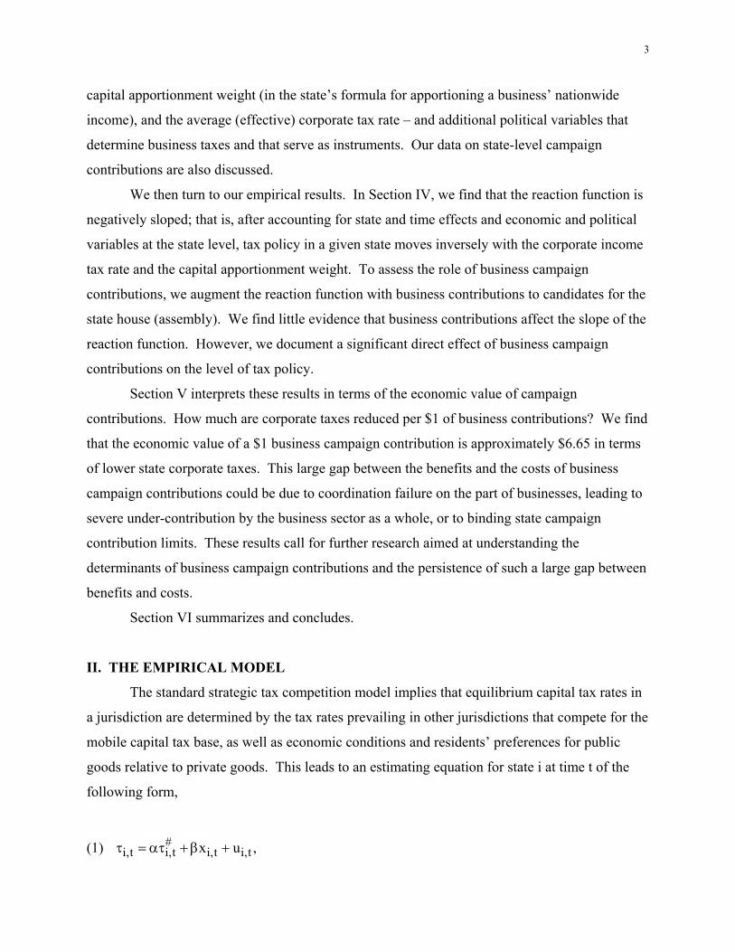
reelection).1 Residents’ utility depends on private and public goods determined by residents’

preferences, businesses’ profit-maximizing decisions, and business tax rates. The expanded

formulation of state policymakers’ welfare recognizes that it is partly influenced by the rent-

seeking behavior of businesses, thus linking business campaign contributions to tax rates.

This departure from the standard strategic tax competition model implies that business campaign

contributions may affect equilibrium tax rates. They may also affect the slope of the tax reaction

function between jurisdictions. Thus, business campaign contributions may directly influence

business tax rates, as well as indirectly shape tax competition, and enhance or retard the mobility

of capital across jurisdictions.

These channels are examined by combining U.S. state panel data on capital tax policy

and other relevant state-level economic and political variables with newly-compiled state-level

data on contributions to candidates for state office. The latter data are constructed from

contribution-level records compiled by the National Institute for Money in State Politics

(NIMSP). These records are required by law to be publicly disclosed and hence cover nearly all

candidates for state office. From these records, we construct at the state level the total amounts

of contributions by type of giver (business vs. non-business), type of office (e.g., house,

governor), and type of candidate (e.g., winning, incumbent). These contributions are sizeable.

During the 2003 to 2006 period, $1.1 billion, or $3.77 per capita, was contributed by the business

sector (defined below) to candidates for state offices. Of these contributions, approximately 33%

went to gubernatorial candidates (including lieutenant governor candidates), another 33% to state

senate candidates, 21% to state house candidates, and the remaining 12% to candidates for other

state offices (e.g., attorneys general and state judges).

Our study begins in Section II with the standard empirical model in the tax competition

literature. The initial empirical results are based on a reaction function relating tax policy in a

given state to tax policies in a competitive set of states and various control variables. We then

augment this model with our business campaign contributions variable.

Our state-level dataset is introduced in Section III. The dataset contains four business tax

variables – the statutory (marginal) corporate income tax rate, the investment tax credit rate, the

1 This formulation of policymakers’ welfare follows Grossman and Helpman (1994, equation (5)) and Edwards and Keen (1996, Section 2). In the latter model, policymakers’ welfare depends on resident utility and “some item of public expenditure…which, while financed from general revenues, benefits only the policymaker…” (p. 118).

3

capital apportionment weight (in the state’s formula for apportioning a business’ nationwide

income), and the average (effective) corporate tax rate – and additional political variables that

determine business taxes and that serve as instruments. Our data on state-level campaign

contributions are also discussed.

We then turn to our empirical results. In Section IV, we find that the reaction function is

negatively sloped; that is, after accounting for state and time effects and economic and political

variables at the state level, tax policy in a given state moves inversely with the corporate income

tax rate and the capital apportionment weight. To assess the role of business campaign

contributions, we augment the reaction function with business contributions to candidates for the

state house (assembly). We find little evidence that business contributions affect the slope of the

reaction function. However, we document a significant direct effect of business campaign

contributions on the level of tax policy.

Section V interprets these results in terms of the economic value of campaign

contributions. How much are corporate taxes reduced per $1 of business contributions? We find

that the economic value of a $1 business campaign contribution is approximately $6.65 in terms

of lower state corporate taxes. This large gap between the benefits and the costs of business

campaign contributions could be due to coordination failure on the part of businesses, leading to

severe under-contribution by the business sector as a whole, or to binding state campaign

contribution limits. These results call for further research aimed at understanding the

determinants of business campaign contributions and the persistence of such a large gap between

benefits and costs.

Section VI summarizes and concludes.

II. THE EMPIRICAL MODEL

The standard strategic tax competition model implies that equilibrium capital tax rates in

a jurisdiction are determined by the tax rates prevailing in other jurisdictions that compete for the

mobile capital tax base, as well as economic conditions and residents’ preferences for public

goods relative to private goods. This leads to an estimating equation for state i at time t of the

following form,

(1) #i,t i,t i,t i,tx u ,

4

where i,t is a tax variable – either the corporate income tax rate, the investment tax credit rate,

the capital apportionment weight, or the average corporate tax rate; #i,t is the tax variable for the

competitive states (the definition of competitive states is discussed in the next section); i,tx is a

set of control variables; i,tu is an error term; and and are parameters to be estimated.

Equation (1) is the standard estimating equation for investigating tax competition, and we

expand on it in five ways.2 First, the error term is assumed to have a two-way error components

structure and equals the sum of a state time-invariant effect ( i ), a time fixed effect ( t ), and a

random error ( i,t ). With regard to the state effects, we present results for both Random Effects

(RE) and Fixed Effects (FE) specifications. Neither estimator dominates. If the state effects are

correlated with the regressors, only FE delivers consistent estimates of the

's and 's .

However, with a panel short in the time dimension, as we have in this paper, the FE estimates

can be estimated imprecisely.3 The RE model, on the other hand, relies on a combination of

cross-section and time-series variation and generates more precise estimates. However, the

consistency of RE estimates requires that the state effects are uncorrelated with the regressors.

Second, we include three variables to control for economic conditions and political preferences:

the investment/capital ratio ( i,t 1IK , which is lagged to avoid problems associated with

simultaneity), the political preferences of state residents ( i,tVOTERPREFERENCES ), and the

investment to capital ratio for the neighboring states (i,t 1

#IK

). These variables are described in

more detail in the next section. Third, the tax competition variable enters with contemporaneous

and two lag values. By including lagged values, we recognize that capital mobility or legislated

changes in tax rates may be gradual processes taking more than one year to complete. Fourth, to

assess the role of business contributions on this tax competition model, we include the logarithm

2 Brueckner (2003), Brueckner and Saavedra (2001), Case, Hines, and Rosen (1993), and Devereux, Lockwood, and Redoano (2008) use a similar estimating equation. 3 The limited variation in the time dimension is traceable to two aspects of our panel data. First, the four tax variables we examine have limited time variation in most states. This is particularly true for the capital apportionment weight, for which changes tend to be of a “one-and-done” nature (i.e., changes occur at most once or twice in the sample for most states). Second, our panel is unbalanced because only a few states have business campaign contributions data before the late 1990s (see the table “Number of States with Reported Business Contributions in NIMSP Data” in Appendix A).

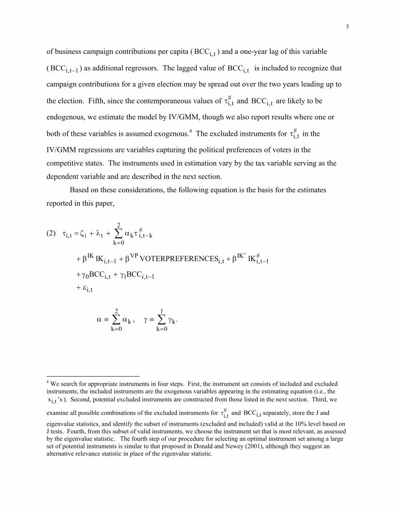
5

of business campaign contributions per capita ( i,tBCC ) and a one-year lag of this variable

( i,t 1BCC ) as additional regressors. The lagged value of i,tBCC is included to recognize that

campaign contributions for a given election may be spread out over the two years leading up to

the election. Fifth, since the contemporaneous values of #i,t and i,tBCC are likely to be

endogenous, we estimate the model by IV/GMM, though we also report results where one or

both of these variables is assumed exogenous.4 The excluded instruments for #i,t in the

IV/GMM regressions are variables capturing the political preferences of voters in the

competitive states. The instruments used in estimation vary by the tax variable serving as the

dependent variable and are described in the next section.

Based on these considerations, the following equation is the basis for the estimates

reported in this paper,

(2) 2

#i,t i t k i,t k

k 0

#IK VP IK #i,t 1 i,t i,t 1

0 i,t 1 i,t 1

i,t

2 1

k kk 0 k 0

IK VOTERPREFERENCES IK

BCC BCC

, .

4 We search for appropriate instruments in four steps. First, the instrument set consists of included and excluded instruments; the included instruments are the exogenous variables appearing in the estimating equation (i.e., the

i,tx 's ). Second, potential excluded instruments are constructed from those listed in the next section. Third, we

examine all possible combinations of the excluded instruments for #i,t and i,tBCC separately, store the J and

eigenvalue statistics, and identify the subset of instruments (excluded and included) valid at the 10% level based on J tests. Fourth, from this subset of valid instruments, we choose the instrument set that is most relevant, as assessed by the eigenvalue statistic. The fourth step of our procedure for selecting an optimal instrument set among a large set of potential instruments is similar to that proposed in Donald and Newey (2001), although they suggest an alternative relevance statistic in place of the eigenvalue statistic.

6

III. THE PANEL DATASET

This section briefly describes the construction of the data used in this study. The series

are for the 48 contiguous U.S. states, cover years from 1988 to 2006 (depending on the state),

and can be set into three categories discussed in the following sub-sections.5

A. Tax and Economic Variables

We examine four state tax policy variables that are referred to in general as i,t . Our

primary focus is on the statutory corporate income tax rate ( i,tSCT ), the investment tax credit

rate ( i,tITC ), and the weight on capital (or property) in the state’s income apportionment formula

( i,tCAW ) because they are controlled directly by legislators. The state corporate income tax rate

is the effective marginal tax rate for the highest bracket of corporate income. The effective

marginal rate is generally lower than the legislated (or statutory) rate due to the deductibility

against federal taxable income of taxes paid to the state. Some states allow full deductibility of

federal corporate income taxes from state taxable income; Iowa and Missouri allow only 50%

deductibility; and some states allow no deductibility at all. It has not generally been recognized

that, owing to deductibility of taxes paid to another level of government, the effective corporate

income tax rates at the state and federal levels are functionally related to each other. These

interrelationships generate two equations in two unknowns, and their solution yields the effective

state corporate income tax rate.

The state investment tax credit is a credit against state corporate income tax liabilities. In

most states, the effective amount of the investment tax credit is simply the legislated investment

tax credit rate multiplied by the value of capital expenditures put into place within the state in a

tax year. The effective rate is lower than the legislated rate in a handful of states for two reasons.

First, five states (Connecticut, Idaho, Maine, North Carolina, and Ohio) permit the state

investment tax credit to be applied only to equipment. For these states, the legislated ITC rate is

multiplied by 2/3, which is approximately the average ratio of equipment capital to total capital

in our data. Second, in some states, the legislated investment tax credit rate varies by the level of

capital expenditures; we use the legislated credit rate for the highest tier of capital expenditures.

5 Alaska and Hawaii are excluded because of the great geographic distance to a neighboring state, thus straining the notion of a “competitive” state as defined by distance between population centroids.

7

The capital apportionment weight is the weight that the state assigns to capital in its

formula for apportioning income among the multiple states in which a firm generates federal

taxable income. Every U.S. state that taxes corporate income uses “formulary apportionment” to

instruct firms that operate in multiple states on allocating their federal taxable income to that

state. The apportionment formula is in all cases a weighted average of the company’s sales,

payroll, and property, though the weight on one or more factor can be and often is equal to zero.

The weights in this formula vary considerably by state. Over the last 30 years, states have

moved toward increasing the weight on sales and decreasing the weights on payroll and property.

These changes encourage job creation and investment in-state and “export” the tax burden to out-

of-state business owners, who sell goods and services in-state but employ workers and capital

out-of-state (Wilson, 2006). The capital apportionment weight can be thought of as a capital tax

instrument with somewhat similar effects as the corporate income tax rate.

Data on CAW are obtained from the following sources. First, data by state for 1997 was

obtained from Edmiston (1998), who compiled the data from the Federation of Tax

Administrators (1997) and generously provided us with an update of these data for 2001.

Second, we use information from Omer and Shelley (2004) documenting when each state first

diverged from the traditional apportionment weights of (1/3, 1/3, 1/3) on payroll, property, and

sales. This information generates a provisional series (assuming no changes between the first

change and 1997 and/or between 1997 and 2001) that we then refine by checking with individual

state tax departments.

The three tax policy measures discussed above have the advantage that they are directly

chosen by state policymakers and hence conform well with our model of strategic tax

competition and business rent-seeking. However, they do not provide a comprehensive measure

of the total tax assessed on capital. A more comprehensive measure would include other taxes

and fees and would account for the ability of business to avoid or mitigate the corporate income

tax by way of various tax planning strategies. Thus, we construct a measure of the average

corporate tax rate ( i,tACT ). This fourth tax policy variable is defined as the ratio of state tax

revenues from corporate taxes, severance taxes, and license fees to total state business income,

the latter measured by gross operating surplus.

The competitive states tax policy ( #i,t ) is an important variable in our analysis and, for

8

state i, is defined as a weighted-average of the tax policies prevailing in the other 47 contiguous

states. This weighted-average formulation is indicated by a superscript “#” and can be

interpreted as a spatial lag on i,t . The weights reflect the "competitive closeness" of the other

states as measured by the inverse distance between the population centroids for a given state and

that of each of the other 47 contiguous states. The weights are normalized to sum to unity.

In the estimating equation, we control for differing economic conditions among states by

including the investment to capital ratio, i,tIK , defined as real investment expenditures in

equipment (excluding software) and structures divided by the constant-dollar replacement value

of the capital stock for the manufacturing sector (NAICS sectors 31 to 33). The capital stock

series is computed according to a perpetual inventory method based on real investment

expenditures, a depreciation rate, and an adjustment to the initial value for book value and

inflation. We measure local economic conditions by investment spending (as opposed to some

other measure of conditions such as the growth in state GDP) because investment conditions

likely have a more direct impact on legislated changes in capital tax rates and because

investment spending better reflects economic conditions prevailing both today and expected to

prevail in the future.

Details concerning the construction and data sources for the series discussed in this sub-

section can be found in the Data Appendix to Chirinko and Wilson (2008).

B. Political Variables

The political preferences of state residents ( i,tVOTERPREFERENCES ) is also a control

variable in the estimating equation and is defined by the extent to which Republicans control the

state government: 0.0 if they control neither the legislature nor governorship, 0.5 if they control

only the legislature or only the governorship, and 1.0 if they control both the legislature and

governorship.

The set of possible instrumental variables for #i,t in the GMM estimation is drawn from

the following list of nine voter preference variables for competitive states. Voter preferences in

competitive states should be relevant instruments – because they affect tax policy in competitive

states for the same reasons that voter preferences in state i affect tax policy in state i – and valid

instruments – because they are unrelated to tax policy in state i (conditional on state and time

9

effects):

(a) the governor is Republican (R). (The complementary class of politicians is

Democrat (D) or Independent (I). An informal examination of the political landscape suggests that Independents tend to be more closely aligned with the Democratic Party. We thus treat D or I politicians as belonging to the same class, DI);

(b) the majority of both houses of the legislature are R; (c) the majority of both houses of the legislature are DI; (d) the governorship changed last year from R to DI; (e) the majority control of the legislature changed last year from DI or split (between R

and DI chambers) to R; (f) an interaction between the R governor and the R legislature indicator variables; (g) an interaction between R governor and the DI legislature indicator variables (note that the omitted interaction category is R governor and a split legislature);

(h) the reelection of an incumbent governor last year; (i) the reelection of a Republican incumbent governor last year.

We form first-order and second-order spatial lags (i.e., weighted averages with the same

distance-weights used in constructing #i,t ) of the above variables as potential instruments. Each

of the four tax variables is projected against different subsets drawn from this set of potential

instruments. The subset used in estimation for each tax variable is the same instrument sets

selected in Chirinko and Wilson (2009b) based on an optimal instrument search algorithm

described in footnote 4. The instrument sets are listed in the Notes To Table 2.


section can be found in the Data Appendix to Chirinko and Wilson (2008).

C. Business Campaign Contributions Variables

The business campaign contributions data are a unique part of this paper. These data are

for contributions made by individuals and organizations to candidates for state office constructed

from contribution-level records compiled by the National Institute for Money in State Politics

10

(NIMSP). The NIMSP assigns each campaign contribution an economic interest code that places

it in a sector. These sectors more or less follow industry classifications but also include labor

organizations, “ideologies,” political parties, etc. We define the “business” supersector as the

sum of the following nine sectors: agriculture; construction; communications and electronics;

defense; energy and natural resources; finance, insurance, and real estate; general business;

transportation; and health. For example, a contribution by a consulting firm or an individual

working at a consulting firm would be credited to the general business sector and counted as a

business contribution. A contribution by a university professor would be credited to the

education sector and would not be counted as a business contribution. Contributions are also

identified as being for a candidate for a particular type of office: state house (H), state senate

(S), or governorship (G). We aggregate all campaign contributions, within each type of office

and within a state, that are assigned to the business sector to get the total dollar amount, $BCCiX,

for each office (X = H, S, G, or the combination HSG). The NIMSP data are an unbalanced

panel. A few states have data beginning in the late 1980s but, for most states, data on

contributions are not available until the late 1990s. The estimates in this paper are based on

business contributions made to candidates for the state house because of our a priori belief that

revenue bills will tend to be initiated in this legislative chamber.6 The business campaign

contributions variable used in the econometric analysis is defined as the logarithm of business

campaign contributions made to candidates for the state house, per capita:

Hi,t i iBCC ln($BCC / POP ) .

The set of possible instrumental variables for i,tBCC in the GMM estimation is drawn

from the following list of six variables based on campaign contributions and the number of

candidates:

6 Ideally, we would also want to assess the effects of senate and gubernatorial contributions on tax policy. However, relative to house elections (where the proportion of seats up for elections is generally the same every two years), senate elections are less frequent and less regular. These characteristics hamper the comparability of state senate contributions data across different years. While regular, gubernatorial elections are even less frequent. This infrequency is reflected in the lumpiness of the data on campaign contributions for gubernatorial candidates, typically positive only every fourth year. Such lumpiness, particularly in a panel with a short time dimension, greatly limits our ability to estimate the effect of gubernatorial contributions on tax policy.

11

(A) the level of campaign contribution limits for corporations to house candidates in that state;

(B) the number of candidates that ran for a state house seat; (C) the amount of non-business campaign contributions to winning candidates;

(D) the amount of non-business contributions to losing candidates;

(E) the ratio of (c) to (d), as a measure of the funding competitiveness of races within the

state;

(F) the amount of business contributions to candidates for other, non-tax-policy-setting state offices (i.e., offices other than governor, state house, or state senate).

The optimal instrument sets for i,tBCC are chosen in the same manner as for #i,t described in

footnote 4. Somewhat surprisingly, the optimal sets for i,tBCC are the same in each of the four

models (which differ by the tax variable serving as the dependent variable) and consists of the

single variable, the number of candidates that ran for a state house seat in state i and year t (item

(B)).


section can be found in Appendix A.

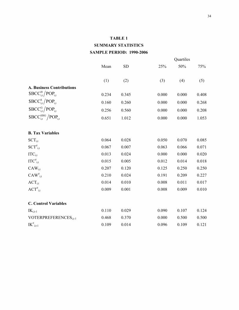
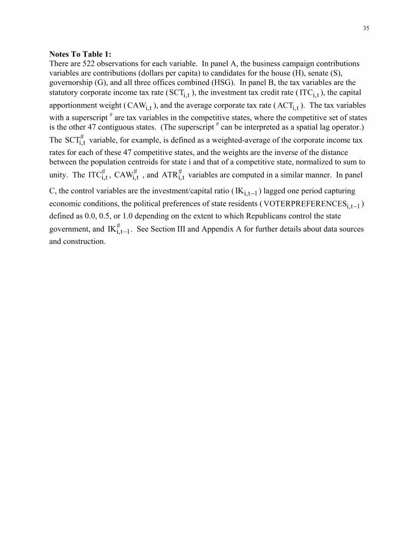
Summary statistics for the business campaign contributions, tax, and control variables are

presented in Table 1. In Panel A, the “H”, “S”, “G”, and “HSG” superscripts on the business

campaign contributions variables ( Xi,t$BCC ) refer to “House,” “Senate,” “Governor,” and

“House, Senate, and Governor combined,” respectively. To ease interpretation, we present

summary statistics for business campaign contributions per capita in levels ( Xi,t i$BCC POP )

rather than logarithms ( Xi,tBCC . There are at least three notable characteristics. First, all of the

business campaign contributions series exhibit a good deal of variation, as standard deviations

exceed their means, yet have zero values for more than 50% of observations (see the quartiles in

columns 3 to 5). Specifically, the proportion of observations with zero values is 53%, 55%, and

63% for house, senate, and gubernatorial contributions (per capita), respectively. This

predominance of zeros is driven in part by the large number of state-years, mostly off-election

12

years in the state, in which there are no business contributions.7 Second, among the tax

variables, i,tITC has the most variation (relative to its mean). Third, the averaging underlying

the definition of the competitive states tax policy and investment/capital ratio variables

(indicated by a superscript #) has a substantial effect in reducing the variation in these variables

relative to their in-state counterparts.

IV. EMPIRICAL RESULTS

A. Tax Competition – Baseline Results

GMM estimates of the standard tax competition model, defined in equation (2) with the

effect of BBC removed (by constraining the 's to equal zero), are presented in Table 2 for three

tax variables – i,tSCT , i,tITC , and i,tCAW – and for Random Effects (RE) and Fixed Effects

(FE) specifications.8 The p-values, based on heteroskedasticity-robust standard errors, are shown

in braces below each coefficient estimate. The instruments for the competitive states tax variable

( #i,t ) vary by tax variable and are listed in the Notes To Tables 2. We begin with the RE

estimates in columns 1 to 3. The sum of the coefficients on #i,t , , measures the slope of the

reaction function and is negative for each of the three tax variables, though they are statistically

insignificant at conventional levels.

Comparable GMM estimates with the RE model are presented in columns 4 to 6. The

’s continue to be negative. In the FE model, the estimated slope of the reaction function –

#i,t i,td / d

– for SCT is now statistically significant at the 10% level and that for CAW has a p-

value only somewhat above 10%. The for ITC is very close to zero. This pattern of results

may be partly explained by the quality of the instruments evaluated in panel C in columns 4, 5,

and 6. For SCT and CAW , the instruments are both valid and relevant, as indicated by the J

Statistic p-value (testing overidentifying restrictions) and the minimum eigenvalue statistic

7 We nonetheless include off-election years in the econometric analysis because tax changes are as likely or more likely to occur in off-election years. For 1990 to 2006, changes in the SCT have occurred 58%/42% of the time in off-election/election years. Comparable figures for the ITC and CAW are 55%/45% and 50%/50%, respectively. Moreover, the inclusion of time lags in our preferred specification requires time-contiguous data. 8 OLS results are presented in Appendix B below and in Chirinko and Wilson (2009a), and they are similar to those reported in Table 2 below.

13

(testing the correlation between #i,t

and the instruments), respectively. The low value of the

latter statistic suggests that the instruments for ITC are weak.

The results from Table 2 indicate that the slopes of the reaction function for SCT and

CAW are negative and suggest the importance of tax competition in determining these capital tax

policies. Though a negatively-sloping reaction function may seem counter-intuitive, it is not

inconsistent with the theory of strategic tax competition and has been found previously in other

empirical work (Chirinko and Wilson, 2009b). The intuition for a negative slope from a model

of strategic tax competition is as follows. Suppose the out-of-state tax rate rises. This increase

will cause mobile capital to flow into the state in question, raising the state’s tax base. If the

income elasticity of residents’ demand for public goods (relative to private goods) is negative,

residents may prefer to use this “windfall” to finance a tax cut, which would result in a negative-

sloping reaction function. In this case, residents view existing public services as adequate and

recognize that, with their now-larger tax base, they can maintain the existing level of public

services at a lower tax rate and shift consumption toward more private goods.

B. The Role of Business Campaign Contributions

The distinctive contribution of this study is to quantify the role of business campaign

contributions on business tax policy. Does i,tBCC impact state tax policies directly? Are

estimates of the reaction function slope affected by the inclusion of i,tBCC in the model? These

impacts are investigated by estimating equation (2) by GMM. The results based on the RE and

FE models are shown in Table 3, columns 1 to 3 and 4 to 6, respectively. The instruments for

#i,tτ are the same as those used in Table 2 For i,tBCC , our instrument search algorithm

(discussed in Section III.C) yields only one instrument, the number of candidates that ran for a

state house seat in state i and year t. Note that the coefficients on i,tBCC and i,t 1BCC , and

their sum represented by , have been multiplied by 1,000 to facilitate presentation.

We find that the introduction of the business contributions variables has little effect on

the estimated slope of the reaction function. The coefficients on #i,tτ could have been biased due

to incorrect omission of BCC. However, the parameters reported in Table 3 are very similar

to those in Table 2. To assess whether BCC influences how jurisdiction react to other

14

jurisdictions’ tax policies, we interact #i,tτ with i,tBCC and, in results not reported here, find no

evidence of any influence of BCC on the slope of the reaction function.

However, we find that business campaign contributions have a direct effect on tax policy

in a direction favorable to business. As shown in Panel B of Table 3, the sign of the estimated

is negative for SCT and CAW, the two tax variables that increase business costs, and is

positive for ITC, the tax policy that lowers business costs. This pattern holds for both the RE

and FE models. In the RE model, is statistically significant (at conventional levels) for both

SCT and CAW, but not for ITC. In the FE model, remains significant for CAW, has a p-value

slightly above 0.10 for SCT, and remains insignificant for ITC.9

The economic significance of these estimates will be assessed in the following section.

Here we simply note that the estimated from column 4 of Table 3 implies that a one standard

deviation (s.d.) movement of BCC is associated with a reduction in SCT of just 0.05 percentage

points (p.p.), which is 2% of the standard deviation of SCT. Similar magnitudes are implied by

the estimated for each of the other two tax variables (from Columns 5 and 6 of Table 3): A

one s.d. movement of BCC is associated with an increase in the ITC of 0.09 p.p. (4% of the ITC

s.d.) and a decrease in the CAW of 0.98 p.p. (8% of the CAW s.d.). As we will show in Section

V, however, even such small movements in tax rates can imply large movements in business

profits, making business campaign contributions a worthwhile investment.

C. Extensions

This subsection extends our empirical results in five directions. First, we have thus far

measured BCC as contributions to candidates for state houses of representatives because house

elections are held every two years and, relative to senate and gubernatorial elections, a continuity

exists across time and states in terms of the fraction of house seats up for election each cycle.

Nonetheless, here we consider whether the results are robust to using a broader measure that

includes contributions to senate and gubernatorial candidates as well. The reaction function

slopes estimated with the RE model are -0.266 (p = 0.519), -0.117 (p = 0.911), and -0.760 (p =

0.135) for SCT, ITC, and CAW, respectively. These estimates are very similar to the

9 We obtain very similar results if we treat BCC as an exogenous variable. The results are provided in Appendix C below and in Chirinko and Wilson (2009a).

15

corresponding results in Columns 1 to 3 of Table 3. The estimated γs are also similar for SCT

and CAW, but the sign for the ITC regression is now negative (though, as before, the coefficient

sum remains statistically insignificant). Specifically, the estimated γs are -0.337 (p = 0.065), -

0.366 (p = 0.663), and -6.014 (p = 0.001) for SCT, ITC, and CAW, respectively.

Second, we explore whether BCC for winning house candidates has different effects on

tax policy than does BCC for losing house candidates. We find statistically insignificant

differences, though this result is driven by the large standard errors on the estimated γwinning and

γlosing coefficients rather than economically similar point estimates. This imprecision appears to

be traceable to the substantial collinearity between BCC for winning and losing candidates.

Third, our preferred model specification contains lags of #i,t to recognize that capital

mobility or legislated changes in tax rates may be gradual processes taking more than one year to

complete. Here we explore the importance of dynamics by considering two alternative

specifications. We first assume that a static specification is appropriate, and thus constrain 1

and 2 to equal zero in equation (2), while estimating 0 freely. The point estimates and

standard errors for α (which now, by definition, equals α0) change dramatically. For example, in

the RE model for CAW, the point estimate for α falls (in absolute value) from −0.926 to −0.274

and the standard error rises by 180%. For SCT and ITC, more dramatic changes occur for α.

For all three tax variables, the estimated γs remain largely unaffected. In the second alternative

specification, we allow for longer lags by replacing the first and second lags of #i,t by a lagged

dependent variable. This specification has the advantage of allowing for infinite number of lags,

but the disadvantages that the weights on the lags must decline geometrically and that the

contemporaneous and lagged effects must be of the same sign, contrary to what we find in our

preferred specification. Estimates of the benchmark model with a lagged dependent variable

replacing the lags of #i,t result in substantial changes in the point estimates and standard errors

for α = α0. Again returning to the example of the RE model for CAW, the point estimate for α

rises from -0.926 to 19.680 and the standard error rises to 119. These problems are attenuated

(point estimate for α of 2.205 with a standard error of 9.194) but not eliminated when we

estimate a hybrid model that combines our preferred specification (two lags of #i,t ) with a

lagged dependent variable. The estimates of γ are also dramatically affected by the inclusion of

16

a lagged dependent variable, with implausible point estimates and very large standard errors.

Neither of these specifications with a lagged dependent variable delivers plausible results for α

or γ.

Fourth, the econometric specifications of tax competition models considered above

focused on tax variables directly controlled by policymakers. However, as noted in Section

III.A, these legislated tax variables do not provide a comprehensive measure of the total tax

assessed on capital and may not reflect nuances in the tax code that affect capital taxation. Table

4 presents results with the average corporate tax rate (ACT) as the tax variable for both RE and

FE specifications. The reaction function slopes continue to be negative, though they are not

estimated very precisely. By contrast, the impact of including BCC in the ACT model is greater

than in the SCT model. Relative to the comparable coefficient sums in Table 3, the γs from

Table 4 are larger -- they imply that a one s.d. movement of BCC is associated with a reduction

in ACT of 7% to 9% of the s.d. of ACT -- and they are estimated more precisely.

Fifth, a major advantage of panel data is that the econometric model can control for state-

specific effects that are time invariant. If these effects are important for tax policy and correlated

with other factors entering the econometric equation, ignoring their impact, as must be done in

cross-section regressions, can lead to very different estimates. To explore the importance of

state-specific effects, we reestimate our models without controlling for random or fixed effects.

The results reported in columns 3 to 5 in Table 4 are very different from the estimates reported

above. For example, recall from Table 3 that γSCT is approximately −0.390 with either a RE or

FE specification with p-values of 0.053 and 0.130, respectively. When state effects are removed,

γSCT switches sign and become statistically insignificant. As shown in column 3 of Table 4, the

estimated sum is 0.495 (p = 0.665). This positive coefficient implies the perverse result that

business campaign contributions are associated with higher corporate income tax rates.

Similarly substantial and perverse changes occur for γITC from its point estimate in Table 3 of

approximately 0.700 to −1.310 (p = 0.381) in Table 4. The γCAW coefficient does not change

sign, but its point estimate changes markedly from approximately -6.660 in Table 3 to −17.180

(p = 0.000) in Table 4. These results highlight the critical importance of controlling for state

effects in panel data.

17

V. THE ECONOMIC VALUE OF BUSINESS CAMPAIGN CONTRIBUTIONS

Up to this point, we have not explored the economic value implied by the BCC

coefficients. How much does a dollar of business contributions “buy” in terms of reduced taxes?

We answer this question with respect to an implied change in the corporate income tax rate. We

focus here only on SCT because the results reported above suggest that BCC does not have a

statistically significant effect on ITC and interpreting the corporate tax savings from a change in

CAW is complicated given it necessarily involves an offsetting increase in the sales or payroll

factor weights in a state’s nationwide income apportionment formula. Moreover, the SCT is

generally considered the most important capital tax policy.

We begin with the following equation for corporate taxes paid,

(3) i i iSCITP ECT *PROFITS ,

i i iECT SCT *RAS

where iSCITP is state corporate income tax payments in state i, iECT is the effective corporate

income tax rate, and iPROFITS is the dollar amount of before-tax corporate profits. The iECT

variable is the product of iSCT (the statutory, marginal corporate income tax rate that enters our

econometric equation) and iRAS (the ratio of the average tax rate to the statutory rate).10 The

economic value of business campaign contributions ( Hi,t$BCC ) is given by the induced savings in

state corporate income tax payments ( i ),

(4) H Hi i i i i i iSCITP / $BCC ( SCT / $BCC )* RAS *PROFITS ,

where we have assumed that the ratio of average to statutory tax rates and before-tax profits are

unaffected by the change in the statutory corporate tax rate. The Hi i( CIT / $BCC ) derivative

10 Note that the iECT variable reflects all aspects of the corporate tax code, and hence differs from the iACT

variable used in Table 4.

18

equals divided by Hi$BCC .11 The iRAS variable is assumed to be the same across states

( iRAS RAS for all i ) because it is measured with national data. Furthermore, we approximate

iPROFITS for a given state as national profits, PROFITS, multiplied by the state’s population

share ( iPOP / POP ). Lastly, we average over the 48 states to calculate the impact of business

contributions for the representative state to obtain the economic value of business contributions,

(5)

48 48H

i i ii 1 i 1

Hi i

/ 48 * POP / $BCC / 48 * RAS * (PROFITS / POP)

.

*MEAN POP / $BCC * RAS * (PROFITS / POP)

The elements appearing in equations (5) are quantified as follows.12 The coefficient is

the fixed effects estimate of -0.375 taken from column 4 of Table 3 (divided by 1,000, per the

Notes To Tables 4 and 5). The Hi iMEAN POP / $BCC equals 6.937, where iPOP and H

i$BCC

are time averages for the most recent four-year election cycle, 2003 to 2006. (All averages

reported in this paragraph are for this period.)13 The PROFITS variable is corporate profits

before tax without the inventory valuation and corporate capital adjustment for the aggregate

economy (U.S. Department of Commerce, Survey of Current Business, Table 1.12); the average

value is $1,401,775 million. The average of the POP variable (Bureau of the Census website) is

294 million. The RAS variable is a ratio. The numerator is computed for the aggregate

economy as average state tax receipts on corporate income ($48,825 million from the U.S.

Department of Commerce, Survey of Current Business, Table 3.3) divided by the above figure

for average aggregate corporate profits before tax. The denominator is average SCT equal to

11 Recall that the business campaign contributions variable in the econometric equation is defined as

Hi,t i,t i,tBCC ln $BCC POP .

12 Equation (5) contains two nominal variables, $BCCH

i and PROFITS. Since they appear in the denominator and numerator, respectively, of equation (5), explicit deflation, which would occur with aggregate deflators, is unnecessary. 13 We focus on this four-year average, rather than the average for the full sample, because of the secular decline in state corporate income tax payments (Wilson, 2006).

19

0.065. The RAS variable is the average of this ratio and equals 0.536.

Based on these numbers and the formula above, business campaign contributions appear

to have considerable economic value. A $1 campaign contribution yields $6.65 in state

corporate tax savings. The result is very similar – $7.00 – if one instead uses the random effects

estimate of (from column 1 of Table 3).

These figures beg the question, if the value of $1 of business campaign contributions is

greater than $1, why do businesses not contribute more, raising contributions until the point at

which the excess return is eliminated?14 There are two possible explanations, which are not

mutually-exclusive, to this “Tullock Puzzle” (1972). First, the above calculation of estimated

economic value is based on the assumption that each business is simultaneously making a

marginal contribution. No mechanism exists, however, for ensuring the substantial mutual gains

are realized. Businesses face a classic free-rider problem with the associated underprovision of a

public good (lobbying).15 In 2008, over 2.5 million tax returns were filed by C and other

corporations with the Internal Revenue Service.16 Among the 48 contiguous states, North

Dakota had the fewest filings, 5,038. With so many corporations even in the smallest states,

appropriate incentives to contribute may be absent and free-riding problems may abound. The

excess return to business contributions may reflect coordination failure among businesses, not

unexploited profit opportunities. Second, campaign contribution limits may effectively constrain

businesses from increasing campaign contributions to the point where their value equals their

cost.

14 Our results contribute to the lively debate concerning whether campaign contributions are an investment by firms for political influence or consumption by participants in the political process. See the survey by Ansolabehere, de Figueiredo, and Snyder (2003) and the evidence that they present in favor of the consumption view. Recent results by Cooper, Gulen, and Ovtchinnikov (2009) favor the investment view; they find a large positive impact of business contributions to federal elections on returns. By contrast, Aggarwal, Meschke, and Wang (2008) find that business contributions to federal elections are negatively related to future returns because of a link between contributions and corporate governance problems. 15 Hardin (1968) and Olson (1965) discuss the difficulties faced by groups in achieving their common interests, though Ostrom (1990) takes a more sanguine view based on the evolution of institutions. 16 The source is the Internal Revenue Service Data Book, 2008, Table 3. These figures exclude S corporations but include other non-C corporations filing form 1120. See footnote 3 of Table 3 for details.

20

VI. SUMMARY AND CONCLUSIONS

This paper has explored the role played by business campaign contributions in

determining state tax policy in a world of mobile capital. We expand the standard model of tax

competition to allow for the influence of business contributions on the corporate income tax rate,

the investment tax credit rate, the capital apportionment weight, and the average corporate tax

rate. Our empirical model explains each of these tax policies as functions of tax policies in

competitive states (reflecting the usual role of tax competition) and business contributions, as

well as control variables for the economic and political environment, state effects, and time fixed

effects.

Based on a panel of U.S. states and unique data on business campaign contributions, our

empirical work uncovers four key results. First, we document a significant direct effect of

business contributions on tax policy. For example, in our preferred regressions in Table 3, we

find that the coefficients on our business campaign contributions variables are negative and

statistically significant at conventional levels (or nearly so in one case) for the statutory corporate

income tax and capital apportionment weight. Second, these estimates imply that the economic

value of a $1 business campaign contribution in terms of lower state corporate taxes is

approximately $6.65. This large gap between the benefits and costs of campaign contributions

suggests that businesses have much to gain from coordinated contributions and/or that campaign

contribution limits have been effective in limiting contributions. Third, the slope of the reaction

function between tax policy in a given state and the tax policies of its competitive states is

negative, and this slope is robust to including business campaign contributions in the

econometric equation. This negative slope reflects a reaction to an inflow of capital (due to an

increase in capital taxes in neighboring jurisdictions) that creates an opportunity for residents to

maintain the current level of public services at a lower tax rate; a negative income elasticity for

public goods compels residents to act on that opportunity. Fourth, we highlight the sensitivity of

the empirical results to state effects. For example, when state effects are removed, the regression

results imply the perverse result that business campaign contributions raise the statutory

corporate income tax rate (column 3 of Table 4).

These provocative results call for further research aimed at understanding the

determinants of business campaign contributions and the “Tullock Puzzle,” the persistence of a

large gap between benefits and costs. What constraints prevent businesses from making

21

additional contributions and exploiting these huge benefits? Are campaign contribution limits

effective in constraining business campaign contributions? We intend to examine these and

related issues in future research.

22

APPENDIX A:

DOCUMENTATION FOR DATA ON BUSINESS CAMPAIGN

CONTRIBUTIONS AND CAMPAIGN CONTRIBUTION LIMITS

Business Campaign Contributions

With financial support from the Federal Reserve Bank of San Francisco, we purchased

data on state campaign contributions from the National Institute of Money in State Politics

(NIMSP). The NIMSP collects data on contributions from individuals and organizations to

individual candidates for state government office. The following statement is from the NIMSP

website (www.followthemoney.org) and describes the sources of their data:

The Institute receives its data in either electronic or paper files from the state disclosure agencies with which candidates must file their campaign finance reports. The Institute collects the information for all state-level candidates in the primary and general elections and then puts it into a database. Staff members verify that all candidates are represented and that their political party affiliations and win/loss statuses are correct. Researchers then standardize the contributor names and assign political donors an economic interest code, based either on the occupation and employer information contained in the disclosure reports or on information found through a variety of research resources. These codes are closely modeled on designations used by the federal government for classifying industry groups. While identifying and coding major labor and industry contributions is relatively straightforward, doing so for individual contributors can be more difficult. In many cases, the state requires that contributors provide the campaigns with their occupation and/or employer. When that information is available, the Institute uses it to assign a category code for individual contributors. When that information is not required or candidates do not provide it, the staff uses standard research tools to determine an economic or political identity. Phone directories provided on CD or through the Internet often include a Standard Industrial Classification for an individual contributor, particularly those who own their own business or are in an easily identifiable profession such as attorney, doctor, insurance salesman, or real estate agent. Professional directories provide additional information, as does Polk's Reverse Directories. Contributors for whom researchers cannot determine an economic interest from the information available receive a code indicating their interest is Unknown.

The NIMSP provided us with the “Summary File” for each state and invaluable

explanations of details about their data. A state’s Summary File contains dollar values of

23

contributions to individual candidates, by year, aggregated across all contributors within a

“sector.” These sectors include industries as well as labor organizations, “ideologies,” political

parties, etc. We define the “business” supersector as the sum of the following nine sectors:

agriculture; construction; communications and electronics; defense; energy and natural

resources; finance, insurance, and real estate; general business; transportation; and health.17

We first aggregate contributions across these nine sectors to obtain business contributions

by candidate, year, and state. Similarly, we aggregate contributions over the remaining sectors to

obtain non-business contributions.

The Summary Files also provide detailed information on the candidate receiving the

donations – in particular, their “office” (e.g., governor, lieutenant governor, house or assembly,

senate, supreme court, attorney general, comptroller, treasurer, public utility commission,

secretary of state, etc.) and “status.” Status indicates the outcome of the candidate’s candidacy

as of the end of the year. Candidacies in the data can have one of the following nine statuses:

general election (GE) win, GE loss, primary election loss, withdrawal, disqualification, death,

unknown, still pending (as of end of year), and “did not run” (meaning the candidate received

contributions in that year but was not running for office that year).

We then aggregate business contributions across candidates, by year and state, for each

status and for four categories of “office”: gubernatorial (includes both governor and lieutenant

governor because in some states these candidates are listed on a joint ticket and so it is not

possible for NIMSP to separate contributions between the gubernatorial candidate and lieutenant

governor candidate), house (variously called by states, “house of assembly”, “house of

delegates”, and “house of representatives”), senate, and other statewide office. In Nebraska,

which has a unicameral state legislature, legislative candidates’ offices are coded as “senate.”

The resulting panel data set has state-year observations on 36 business campaign

contributions variables: contributions to candidates for each of the four offices above and for

each of the nine statuses above.

17 The above description by the NIMSP of their extensive efforts to assign contributions from individuals to a particular economic sector, may lead one to think that contributions from individuals, as opposed to organizations, is the bulk of business contributions. They are not. According to the breakdown of contributions by individuals vs. organizations provided on the NIMSP website, individuals make up around a third to a half of business contributions (depending on the state and year).

24

From these 36 business campaign contribution variables, we construct the following

variables for possible use in our analysis:

Explanatory Variables

H$BCC – business contributions-house

S$BCC – business contributions-senate

G$BCC – business contributions-governor/lieutenant governor

HSG$BCC – business contributions-house + senate + governor

Possible Instrumental Variables

W$NBC – non-business contributions-house-GE winners

L$NBC – non-business contributions-house-GE losers

$NBC – non-business contributions-house-GE winners + GE losers

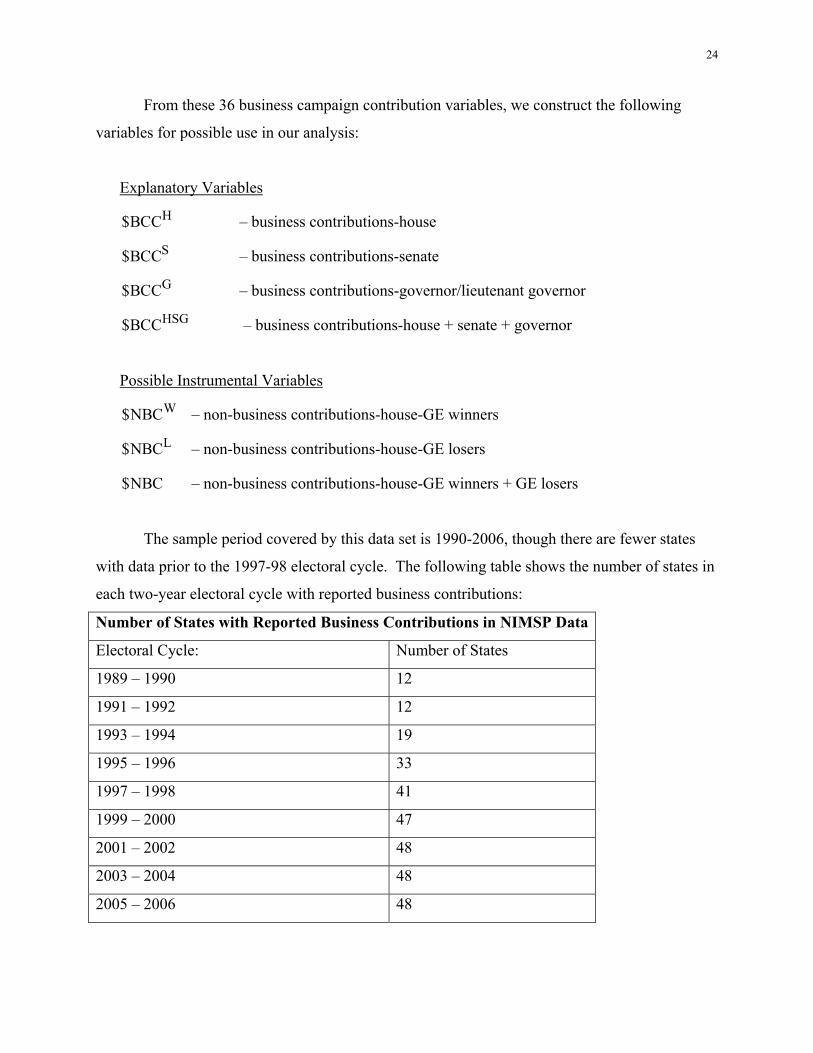
The sample period covered by this data set is 1990-2006, though there are fewer states

with data prior to the 1997-98 electoral cycle. The following table shows the number of states in

each two-year electoral cycle with reported business contributions:

Number of States with Reported Business Contributions in NIMSP Data

Electoral Cycle: Number of States

1989 – 1990 12

1991 – 1992 12

1993 – 1994 19

1995 – 1996 33

1997 – 1998 41

1999 – 2000 47

2001 – 2002 48

2003 – 2004 48

2005 – 2006 48

25

As indicated by the table above, contributions data in the NIMSP data set are not reported for all

states in all years.

States can be categorized into four groups to describe their data availability: 1. Most (40 of 48) states have only even-year data on business contributions. These states

have biennial electoral cycles that end in even-years and report contributions over the entire two-year period in that single even-year.

2. Two states – New Jersey and Virginia – have only odd-year contributions data; they have

biennial electoral cycles ending in odd-years and report contributions over the entire two-year period in that single odd-year.

3. Five states – Kentucky, Louisiana, Mississippi, Pennsylvania, and Wisconsin – have

biennial, even-year elections but report contributions that take place in either election years or non-election (odd) years. For these states, off-election-year contributions generally are for statewide offices other than governor, house, or senate (so governor, house, or senate contributions generally are just for even years, like the 40 states in the first group above).

4. California has a biennial, even-year cycle like group 1 above but has contributions

reported for 2003 in connection with the special gubernatorial recall election in that year.

Since most states only report contributions at a two-year, electoral-cycle frequency, it is not

known how contributions are divided among the two years within a cycle. If non-election-year

contributions are generally close to zero, then the appropriate way to handle the data is to assign

all of the contributions for the cycle to the election year and assume unreported contributions are

0 in non-election years. In this case, the data set constructed at an annual frequency is

appropriate for the purposes of our regression analysis.

Campaign Contributions Limits

There are at least six different kinds of campaign contribution limits (CCLs): (1) on

corporate contributions, (2) on individual contributions, (3) on candidates’ own and family

contributions, (4) on political action committee (PAC) contributions, (5) on labor union

contributions, and (6) on contributions by political parties.

The basic principle we use for constructing a uniform panel of data for these six types of

CCLs is as follows: “What is the maximum amount that a contributor (individual, corporation,

candidate, PAC, union, or party) could make to a single candidate in this state in this electoral

26

cycle?” There are two main categories of CCLs: CCLs that set a maximum contribution limit

from a single contributor to a specific candidate (the easiest case to record in our dataset), and

CCLs that cap aggregate contributions from a single contributor to all candidates seeking a

particular office, such as governor or state senate. In the latter case, we assume that the

contributor would use their entire allowable donation (if binding) for one candidate, to maximize

impact. Contribution maximums in the dataset specify the most a contributor can contribute in a

particular election cycle, which includes both the primary and general elections. In states where

the limit applies on a calendar-year basis, we multiply it by 2 to be (roughly) equivalent to a

primary/general cycle.

Nebraska is a special case, where candidates are limited in the total amount they can

receive in corporate donations. The assumption used to enter this information in our dataset is

that one donor can give an amount equal to this maximum (e.g., $825,000 for governor).

There have been a number of court cases on whether particular campaign finance limits

are unconstitutional, which is a primarily reason for the large amount of within-state variation in

CCLs over time. Some states (e.g., Colorado) abandoned all limits for 2 years, then rolled out

new ones that presumably passed Constitutional muster. This is one reason to think CCLs are

exogenous with respect to a state’s tax policy.

In a handful of states, the maximum contribution limit is higher if the candidate agrees to

spending limits (New Hampshire) or is qualified to receive public funding (Rhode Island). In

these cases, we assume that these higher limits apply.

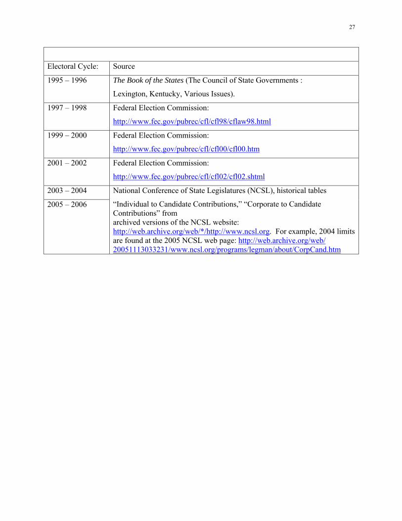
Our data sources for CCLs are as follows:

27

Electoral Cycle: Source

1995 – 1996 The Book of the States (The Council of State Governments :

Lexington, Kentucky, Various Issues).

1997 – 1998 Federal Election Commission:

http://www.fec.gov/pubrec/cfl/cfl98/cflaw98.html


http://www.fec.gov/pubrec/cfl/cfl00/cfl00.htm


http://www.fec.gov/pubrec/cfl/cfl02/cfl02.shtml

2003 – 2004 National Conference of State Legislatures (NCSL), historical tables

“Individual to Candidate Contributions,” “Corporate to Candidate Contributions” from archived versions of the NCSL website: http://web.archive.org/web/*/http://www.ncsl.org. For example, 2004 limits are found at the 2005 NCSL web page: http://web.archive.org/web/ 20051113033231/www.ncsl.org/programs/legman/about/CorpCand.htm

2005 – 2006

28

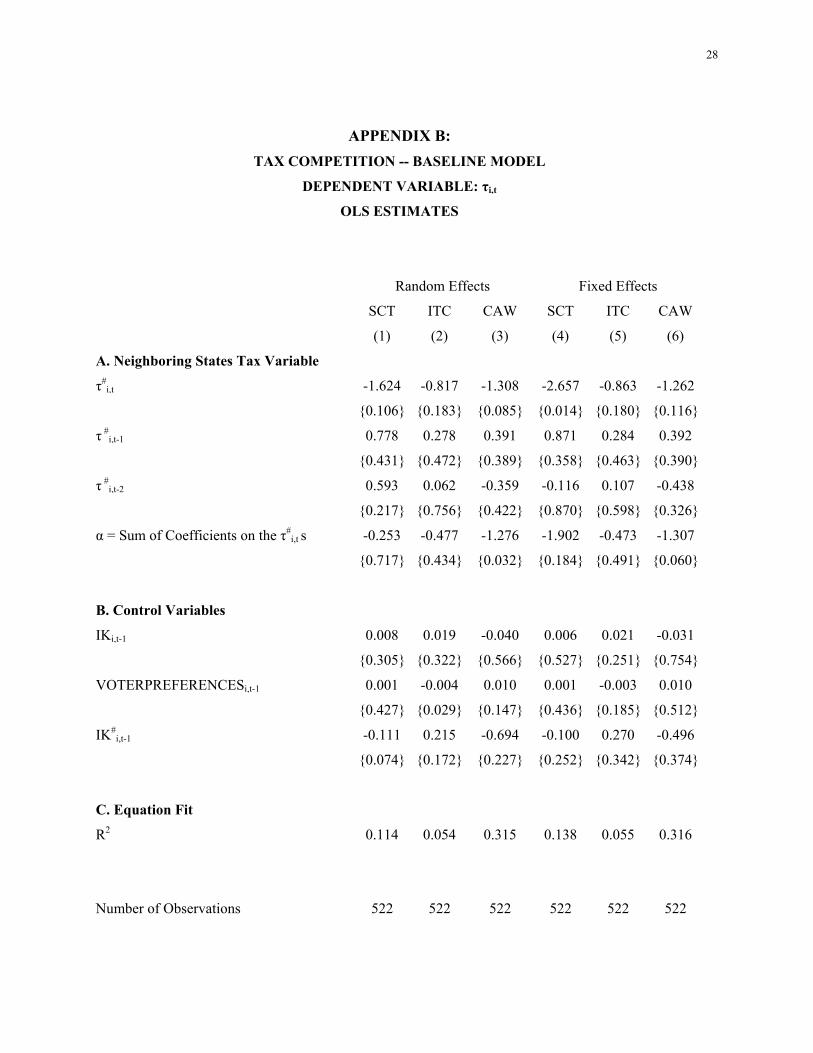
APPENDIX B:

TAX COMPETITION -- BASELINE MODEL

DEPENDENT VARIABLE: τi,t

OLS ESTIMATES

Random Effects Fixed Effects

SCT ITC CAW SCT ITC CAW

(1) (2) (3) (4) (5) (6)

A. Neighboring States Tax Variable

τ#i,t -1.624 -0.817 -1.308 -2.657 -0.863 -1.262

{0.106} {0.183} {0.085} {0.014} {0.180} {0.116}

τ #i,t-1 0.778 0.278 0.391 0.871 0.284 0.392

{0.431} {0.472} {0.389} {0.358} {0.463} {0.390}

τ #i,t-2 0.593 0.062 -0.359 -0.116 0.107 -0.438

{0.217} {0.756} {0.422} {0.870} {0.598} {0.326}

α = Sum of Coefficients on the τ#i,t s -0.253 -0.477 -1.276 -1.902 -0.473 -1.307

{0.717} {0.434} {0.032} {0.184} {0.491} {0.060}

B. Control Variables

IKi,t-1 0.008 0.019 -0.040 0.006 0.021 -0.031

{0.305} {0.322} {0.566} {0.527} {0.251} {0.754}

VOTERPREFERENCESi,t-1 0.001 -0.004 0.010 0.001 -0.003 0.010

{0.427} {0.029} {0.147} {0.436} {0.185} {0.512}

IK#i,t-1 -0.111 0.215 -0.694 -0.100 0.270 -0.496

{0.074} {0.172} {0.227} {0.252} {0.342} {0.374}

C. Equation Fit

R2 0.114 0.054 0.315 0.138 0.055 0.316

Number of Observations 522 522 522 522 522 522

29

Notes To Appendix B: OLS estimates are based on equation (2) with panel data for 48 states for the period 1990 to 2006. Columns 1, 2, and 3 treat state effects as random variables; columns 4, 5, and 6 treat state effects as fixed effects. All models contain time fixed effects. The results are comparable to those in Table 2 and differ only by the method of estimation. See the Notes To Tables 1 and 2 for details about the table entries.

30

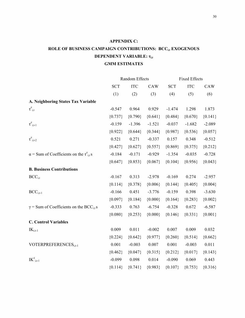
APPENDIX C:

ROLE OF BUSINESS CAMPAIGN CONTRIBUTIONS: BCCi,t EXOGENOUS


GMM ESTIMATES



(1) (2) (3) (4) (5) (6)


τ#i,t -0.547 0.964 0.929 -1.474 1.298 1.873

{0.737} {0.790} {0.641} {0.484} {0.670} {0.141}

τ#i,t-1 -0.159 -1.396 -1.521 -0.037 -1.682 -2.089

{0.922} {0.644} {0.344} {0.987} {0.536} {0.057}

τ#i,t-2 0.521 0.271 -0.337 0.157 0.348 -0.512

{0.427} {0.627} {0.557} {0.869} {0.375} {0.212}


{0.647} {0.853} {0.067} {0.104} {0.956} {0.043}

B. Business Contributions

BCCi,t -0.167 0.313 -2.978 -0.169 0.274 -2.957

{0.114} {0.378} {0.006} {0.144} {0.405} {0.004}

BCCi,t-1 -0.166 0.451 -3.776 -0.159 0.398 -3.630

{0.097} {0.184} {0.000} {0.164} {0.283} {0.002}

γ = Sum of Coefficients on the BCCi,t s -0.333 0.763 -6.754 -0.328 0.672 -6.587

{0.080} {0.253} {0.000} {0.146} {0.331} {0.001}

C. Control Variables

IKi,t-1 0.009 0.011 -0.002 0.007 0.009 0.032

{0.224} {0.642} {0.977} {0.260} {0.514} {0.662}


{0.462} {0.047} {0.315} {0.212} {0.017} {0.143}

IK#i,t-1 -0.099 0.098 0.014 -0.090 0.069 0.443

{0.114} {0.741} {0.983} {0.107} {0.753} {0.316}

31

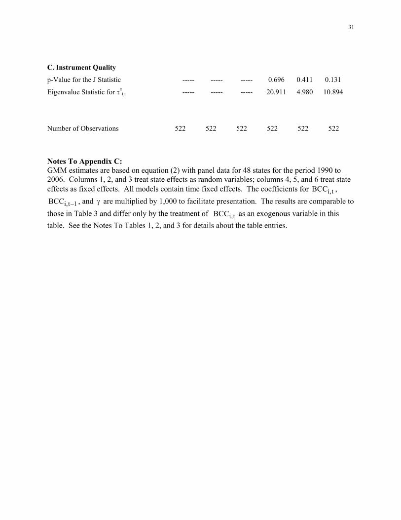
C. Instrument Quality

p-Value for the J Statistic ----- ----- ----- 0.696 0.411 0.131

Eigenvalue Statistic for τ#i,t ----- ----- ----- 20.911 4.980 10.894


Notes To Appendix C: GMM estimates are based on equation (2) with panel data for 48 states for the period 1990 to 2006. Columns 1, 2, and 3 treat state effects as random variables; columns 4, 5, and 6 treat state effects as fixed effects. All models contain time fixed effects. The coefficients for i,tBCC ,

i,t 1BCC , and are multiplied by 1,000 to facilitate presentation. The results are comparable to

those in Table 3 and differ only by the treatment of i,tBCC as an exogenous variable in this

table. See the Notes To Tables 1, 2, and 3 for details about the table entries.

32

REFERENCES

Aggarwal, Rajesh K., Felix Meschke, and Tracy Wang, Tracy, 2008. “Corporate Political

Contributions: Investment or Agency?” University of Minnesota.

Ansolabehere, Stephen, John M. de Figueiredo, , James M. Snyder, Jr., 2003. “Why Is There So Little Money in U.S. Politics?” Journal of Economic Perspectives 17 (1), 105-130.

Brueckner, Jan K., 2003. "Strategic Interaction Among Governments: An Overview of Empirical Studies." International Regional Science Review 26 (2), 175-188.

Brueckner, Jan K., and Luz A. Saavedra, 2001. "Do Local Governments Engage In Strategic Property-Tax Competition?" National Tax Journal 54 (2), 203-229.

Case, Anne C., James R. Jr. Hines, and Harvey S. Rosen, 1993. "Budget Spillovers and Fiscal Policy Interdependence: Evidence From the States." Journal of Public Economics 52 (3), 285-307.

Chirinko, Robert S., and Daniel J. Wilson, 2008. “State Investment Tax Incentives: A Zero- Sum Game?” Journal of Public Economics 92 (12), 2362-2384. Chirinko, Robert S., and Daniel J. Wilson, 2009a. “Can Lower Tax Rates Be Bought? Business

Rent-Seeking and Tax Competition Among U.S. States.” Federal Reserve Bank of San Francisco Working Paper No. 2009-29 and University of Illinois at Chicago.

Chirinko, Robert S., and Daniel J. Wilson, 2009b. “Tax Competition among U.S. States: Racing

to the Bottom or Riding on a Seesaw?” Federal Reserve Bank of San Francisco Working Paper No. 2008-03 and University of Illinois at Chicago.

Cooper, Michael J., Huseyin Gulen,, and Alexei V. Ovtchinnikov, 2009. “Corporate Political

Contributions and Stock Returns.” University of Utah, Purdue University, and Vanderbilt University.

Devereux, Michael P., Ben Lockwood, and Michela Redoano, 2008. "Do Countries Compete

Over Corporate Tax Rates?" Journal of Public Economics 92 (5-6), 1210-1235.

Donald, Stephen G., and Whitney K. Newey, 2001. “Choosing the Number of Instruments.” Econometrica 69 (5), 1161-1191.

Edmiston, Kelly D., 1998. “Formula-Apportioned Corporate Income Taxes and Regional Economic Development.” Doctoral Dissertation, University of Tennessee.

Edwards, Jeremy, and Michael Keen, 1996, “Tax Competition and Leviathan.” European Economic Review 40 (1), 113-134.

Federation of Tax Administrators, 1997. "State Apportionment of Corporate Income," Access 1997 at http://www.taxadmin.org/fta/rate/corp_app.html.

33

Grossman, Gene M., and Elhanan Helpman, 1994. “Protection for Sale.” American Economic Review 84 (4), 833-850. Hansen, Lars P., 1982. “Large Sample Properties of Generalized Method of Moments Estimators.” Econometrica 50 (4), 1029-1054. Hardin, Garrett, 1968. “Tragedy of the Commons.” Science 162, 1243-1248. Internal Revenue Service, U.S. Department of the Treasury. Internal Revenue Service Data Book 2008. Internal Revenue Service website: http://www.irs.gov/taxstats/article/0,,id=102174,00.html Olson, Mancur, 1965. The Logic of Collective Action: Public Goods and the Theory of Groups.

Harvard University Press, Cambridge, MA.

Omer, Thomas C., and Marjorie K. Shelley, 2004. Competitive, Political, and Economic Factors Influencing State Tax Policy Changes.” Journal of American Tax Association 26 (Supplement), 103-126.

Ostrom, Elinor, 1990. Governing the Commons: The Evolution of Institutions for Collective Action. Cambridge University Press, Cambridge, UK.

Stock, James H., Wright, Jonathan H., and Yogo, Motohiro, 2002. "A Survey of Weak Instruments and Weak Identification in Generalized Method of Moments." Journal of Business & Economic Statistics 20 (4), 518-529.

Stock, James H., and Yogo, Motohiro, 2005. "Testing for Weak Instruments in Linear IV Regression." In Andrews, Donald W.K. and James H. Stock (eds.). Identification and Inference for Econometric Models: Essays in Honor of Thomas Rothenberg. Cambridge University Press, Cambridge, UK, 80-108.

Tullock, Gordon, 1972. “The Purchase of Politicians.” Western Economic Journal 10 (3), 354-355.

U.S. Bureau of the Census, U.S. Department of Commerce. URL: http://www.census.gov. U.S. Department of Commerce, Survey of Current Business. URL: http://www.bea.gov. White, Halbert, 1980. "A Heteroskedasticity-Consistent Covariance Matrix Estimator and a

Direct Test for Heteroskedasticity." Econometrica 48 (4), 817-838. White, Halbert, 1982. "Instrumental Variables Regression with Independent Observations," Econometrica 50 (2), 483-500. Wilson, Daniel J., 2006. “The Mystery of Falling State Corporate Income Taxes.” Federal

Reserve Bank of San Francisco Economic Letter 2006-35.

34

TABLE 1

SUMMARY STATISTICS

SAMPLE PERIOD: 1990-2006

Quartiles

Mean SD 25% 50% 75%

(1) (2) (3) (4) (5)

A. Business Contributions Hi,t i,t$BCC POP 0.234 0.345 0.000 0.000 0.408 Si,t i,t$BCC POP 0.160 0.260 0.000 0.000 0.268 Gi,t i,t$BCC POP 0.256 0.560 0.000 0.000 0.208 HSGi,t i,t$BCC POP 0.651 1.012 0.000 0.000 1.053

B. Tax Variables

SCTi,t 0.064 0.028 0.050 0.070 0.085

SCT#i,t 0.067 0.007 0.063 0.066 0.071

ITCi,t 0.013 0.024 0.000 0.000 0.020

ITC#i,t 0.015 0.005 0.012 0.014 0.018

CAWi,t 0.207 0.120 0.125 0.250 0.250

CAW#i,t 0.210 0.024 0.191 0.209 0.227

ACTi,t 0.014 0.010 0.008 0.011 0.017

ACT#i,t 0.009 0.001 0.008 0.009 0.010


IKi,t-1 0.110 0.029 0.090 0.107 0.124

VOTERPREFERENCESi,t-1 0.468 0.370 0.000 0.500 0.500

IK#i,t-1 0.109 0.014 0.096 0.109 0.121

35

Notes To Table 1: There are 522 observations for each variable. In panel A, the business campaign contributions variables are contributions (dollars per capita) to candidates for the house (H), senate (S), governorship (G), and all three offices combined (HSG). In panel B, the tax variables are the statutory corporate income tax rate ( i,tSCT ), the investment tax credit rate ( i,tITC ), the capital

apportionment weight ( i,tCAW ), and the average corporate tax rate ( i,tACT ). The tax variables

with a superscript # are tax variables in the competitive states, where the competitive set of states is the other 47 contiguous states. (The superscript # can be interpreted as a spatial lag operator.)

The #i,tSCT variable, for example, is defined as a weighted-average of the corporate income tax

rates for each of these 47 competitive states, and the weights are the inverse of the distance between the population centroids for state i and that of a competitive state, normalized to sum to

unity. The #i,tITC , #

i,tCAW , and #i,tATR variables are computed in a similar manner. In panel

C, the control variables are the investment/capital ratio ( i,t 1IK ) lagged one period capturing

economic conditions, the political preferences of state residents ( i,t 1VOTERPREFERENCES )

defined as 0.0, 0.5, or 1.0 depending on the extent to which Republicans control the state

government, and #i,t 1IK . See Section III and Appendix A for further details about data sources

and construction.

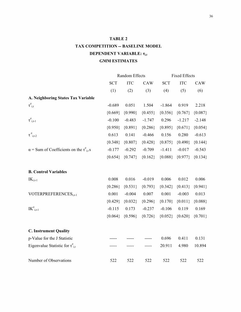
36

TABLE 2

TAX COMPETITION -- BASELINE MODEL


GMM ESTIMATES



(1) (2) (3) (4) (5) (6)


τ#i,t -0.689 0.051 1.504 -1.864 0.919 2.218

{0.669} {0.990} {0.455} {0.356} {0.767} {0.087}

τ#i,t-1 -0.100 -0.483 -1.747 0.296 -1.217 -2.148

{0.950} {0.891} {0.286} {0.895} {0.671} {0.054}

τ #i,t-2 0.613 0.141 -0.466 0.156 0.280 -0.613

{0.348} {0.807} {0.428} {0.875} {0.490} {0.144}


{0.654} {0.747} {0.162} {0.088} {0.977} {0.134}

B. Control Variables

IKi,t-1 0.008 0.016 -0.019 0.006 0.012 0.006

{0.286} {0.531} {0.793} {0.342} {0.413} {0.941}


{0.429} {0.032} {0.296} {0.170} {0.011} {0.088}

IK#i,t-1 -0.115 0.173 -0.237 -0.106 0.119 0.169

{0.064} {0.596} {0.726} {0.052} {0.620} {0.701}

C. Instrument Quality




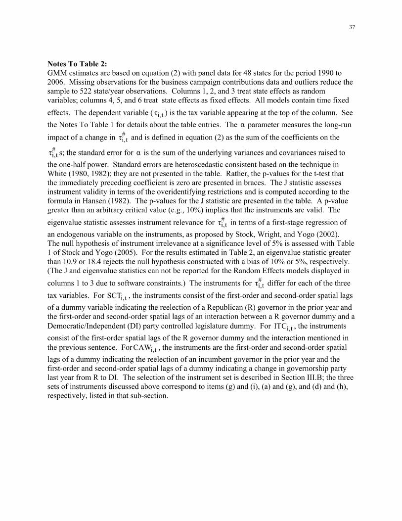
37

Notes To Table 2: GMM estimates are based on equation (2) with panel data for 48 states for the period 1990 to 2006. Missing observations for the business campaign contributions data and outliers reduce the sample to 522 state/year observations. Columns 1, 2, and 3 treat state effects as random variables; columns 4, 5, and 6 treat state effects as fixed effects. All models contain time fixed

effects. The dependent variable ( i,tτ ) is the tax variable appearing at the top of the column. See

the Notes To Table 1 for details about the table entries. The α parameter measures the long-run

impact of a change in #i,tτ and is defined in equation (2) as the sum of the coefficients on the

#i,tτ s; the standard error for α is the sum of the underlying variances and covariances raised to

the one-half power. Standard errors are heteroscedastic consistent based on the technique in White (1980, 1982); they are not presented in the table. Rather, the p-values for the t-test that the immediately preceding coefficient is zero are presented in braces. The J statistic assesses instrument validity in terms of the overidentifying restrictions and is computed according to the formula in Hansen (1982). The p-values for the J statistic are presented in the table. A p-value greater than an arbitrary critical value (e.g., 10%) implies that the instruments are valid. The

eigenvalue statistic assesses instrument relevance for #i,tτ in terms of a first-stage regression of

an endogenous variable on the instruments, as proposed by Stock, Wright, and Yogo (2002). The null hypothesis of instrument irrelevance at a significance level of 5% is assessed with Table 1 of Stock and Yogo (2005). For the results estimated in Table 2, an eigenvalue statistic greater than 10.9 or 18.4 rejects the null hypothesis constructed with a bias of 10% or 5%, respectively. (The J and eigenvalue statistics can not be reported for the Random Effects models displayed in

columns 1 to 3 due to software constraints.) The instruments for #i,tτ differ for each of the three

tax variables. For i,tSCT , the instruments consist of the first-order and second-order spatial lags

of a dummy variable indicating the reelection of a Republican (R) governor in the prior year and the first-order and second-order spatial lags of an interaction between a R governor dummy and a Democratic/Independent (DI) party controlled legislature dummy. For i,tITC , the instruments

consist of the first-order spatial lags of the R governor dummy and the interaction mentioned in the previous sentence. For i,tCAW , the instruments are the first-order and second-order spatial

lags of a dummy indicating the reelection of an incumbent governor in the prior year and the first-order and second-order spatial lags of a dummy indicating a change in governorship party last year from R to DI. The selection of the instrument set is described in Section III.B; the three sets of instruments discussed above correspond to items (g) and (i), (a) and (g), and (d) and (h), respectively, listed in that sub-section.

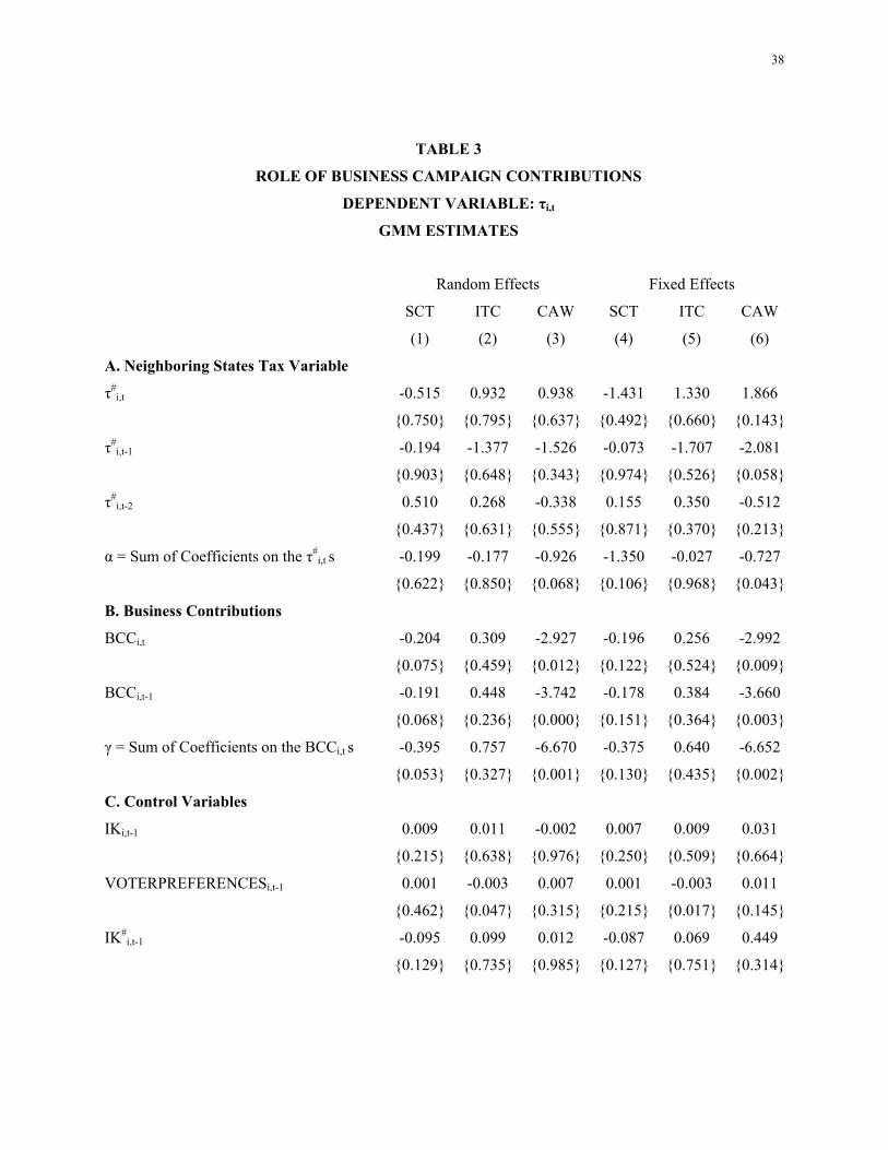
38

TABLE 3

ROLE OF BUSINESS CAMPAIGN CONTRIBUTIONS


GMM ESTIMATES



(1) (2) (3) (4) (5) (6)


τ#i,t -0.515 0.932 0.938 -1.431 1.330 1.866

{0.750} {0.795} {0.637} {0.492} {0.660} {0.143}

τ#i,t-1 -0.194 -1.377 -1.526 -0.073 -1.707 -2.081

{0.903} {0.648} {0.343} {0.974} {0.526} {0.058}

τ#i,t-2 0.510 0.268 -0.338 0.155 0.350 -0.512

{0.437} {0.631} {0.555} {0.871} {0.370} {0.213}


{0.622} {0.850} {0.068} {0.106} {0.968} {0.043}


BCCi,t -0.204 0.309 -2.927 -0.196 0.256 -2.992

{0.075} {0.459} {0.012} {0.122} {0.524} {0.009}

BCCi,t-1 -0.191 0.448 -3.742 -0.178 0.384 -3.660

{0.068} {0.236} {0.000} {0.151} {0.364} {0.003}

γ = Sum of Coefficients on the BCCi,t s -0.395 0.757 -6.670 -0.375 0.640 -6.652

{0.053} {0.327} {0.001} {0.130} {0.435} {0.002}


IKi,t-1 0.009 0.011 -0.002 0.007 0.009 0.031

{0.215} {0.638} {0.976} {0.250} {0.509} {0.664}


{0.462} {0.047} {0.315} {0.215} {0.017} {0.145}

IK#i,t-1 -0.095 0.099 0.012 -0.087 0.069 0.449

{0.129} {0.735} {0.985} {0.127} {0.751} {0.314}

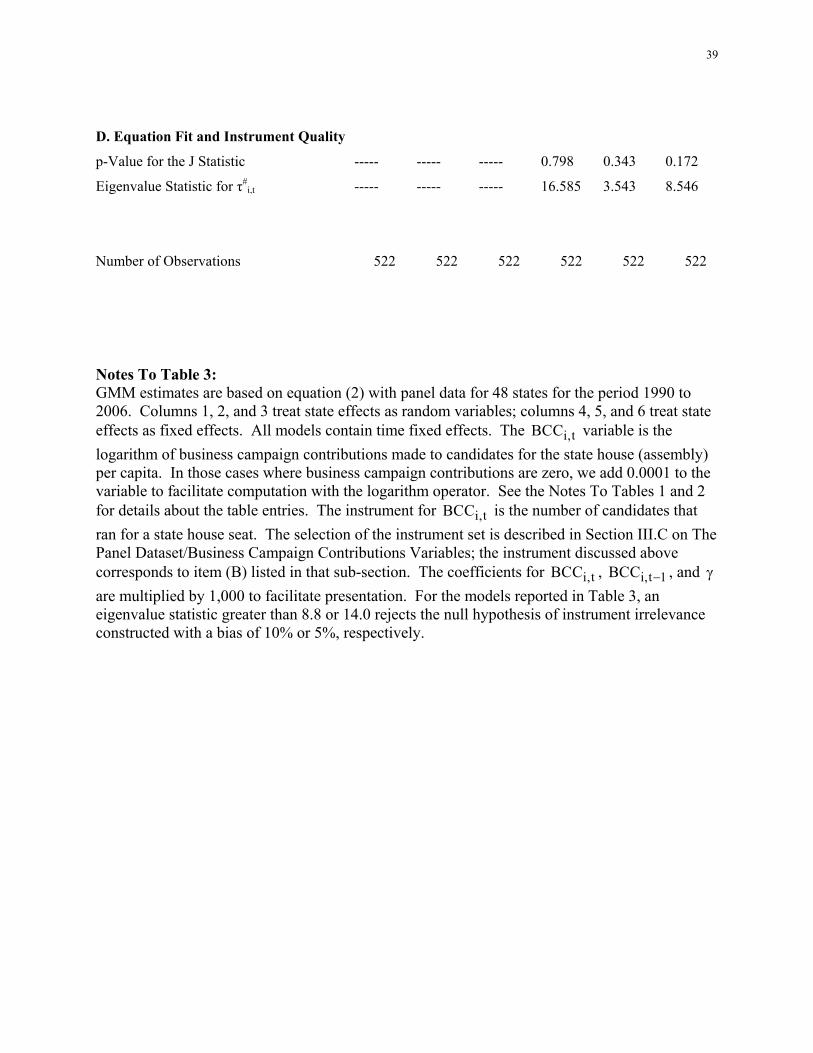
39

D. Equation Fit and Instrument Quality




Notes To Table 3: GMM estimates are based on equation (2) with panel data for 48 states for the period 1990 to 2006. Columns 1, 2, and 3 treat state effects as random variables; columns 4, 5, and 6 treat state effects as fixed effects. All models contain time fixed effects. The i,tBCC variable is the

logarithm of business campaign contributions made to candidates for the state house (assembly) per capita. In those cases where business campaign contributions are zero, we add 0.0001 to the variable to facilitate computation with the logarithm operator. See the Notes To Tables 1 and 2 for details about the table entries. The instrument for i,tBCC is the number of candidates that

ran for a state house seat. The selection of the instrument set is described in Section III.C on The Panel Dataset/Business Campaign Contributions Variables; the instrument discussed above corresponds to item (B) listed in that sub-section. The coefficients for i,tBCC , i,t 1BCC , and

are multiplied by 1,000 to facilitate presentation. For the models reported in Table 3, an eigenvalue statistic greater than 8.8 or 14.0 rejects the null hypothesis of instrument irrelevance constructed with a bias of 10% or 5%, respectively.

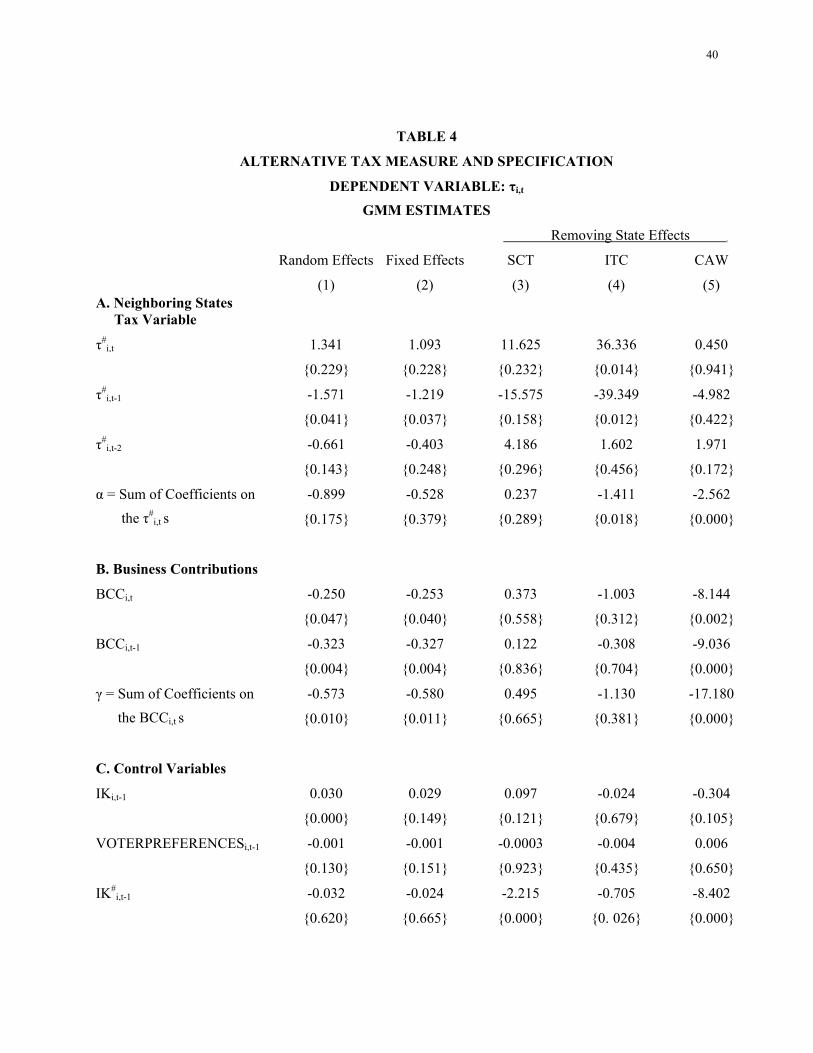
40

TABLE 4

ALTERNATIVE TAX MEASURE AND SPECIFICATION


GMM ESTIMATES

Removing State Effects .

Random Effects Fixed Effects SCT ITC CAW

(1) (2) (3) (4) (5) A. Neighboring States Tax Variable

τ#i,t 1.341 1.093 11.625 36.336 0.450

{0.229} {0.228} {0.232} {0.014} {0.941}

τ#i,t-1 -1.571 -1.219 -15.575 -39.349 -4.982

{0.041} {0.037} {0.158} {0.012} {0.422}

τ#i,t-2 -0.661 -0.403 4.186 1.602 1.971

{0.143} {0.248} {0.296} {0.456} {0.172}

α = Sum of Coefficients on

the τ#i,t s

-0.899 -0.528 0.237 -1.411 -2.562

{0.175} {0.379} {0.289} {0.018} {0.000}


BCCi,t -0.250 -0.253 0.373 -1.003 -8.144

{0.047} {0.040} {0.558} {0.312} {0.002}

BCCi,t-1 -0.323 -0.327 0.122 -0.308 -9.036

{0.004} {0.004} {0.836} {0.704} {0.000}

γ = Sum of Coefficients on

the BCCi,t s

-0.573 -0.580 0.495 -1.130 -17.180

{0.010} {0.011} {0.665} {0.381} {0.000}


IKi,t-1 0.030 0.029 0.097 -0.024 -0.304

{0.000} {0.149} {0.121} {0.679} {0.105}

VOTERPREFERENCESi,t-1 -0.001 -0.001 -0.0003 -0.004 0.006

{0.130} {0.151} {0.923} {0.435} {0.650}

IK#i,t-1 -0.032 -0.024 -2.215 -0.705 -8.402

{0.620} {0.665} {0.000} {0. 026} {0.000}

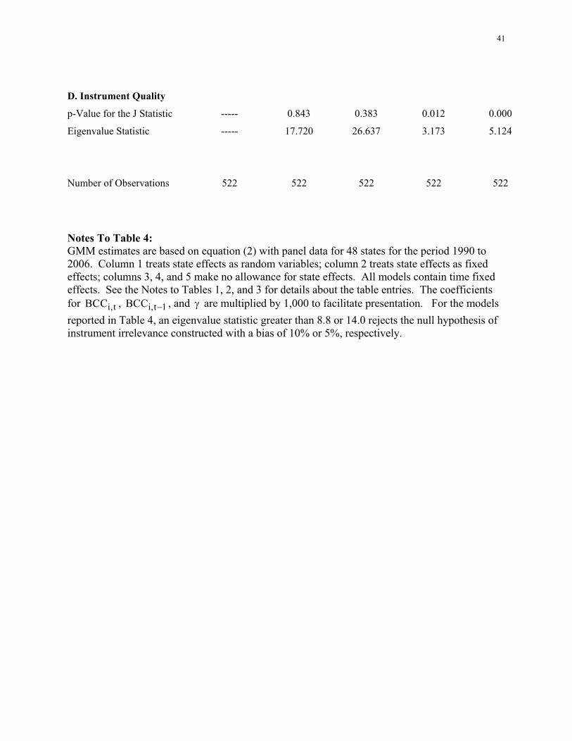
41

D. Instrument Quality

p-Value for the J Statistic ----- 0.843 0.383 0.012 0.000

Eigenvalue Statistic ----- 17.720 26.637 3.173 5.124

Number of Observations 522 522 522 522 522

Notes To Table 4: GMM estimates are based on equation (2) with panel data for 48 states for the period 1990 to 2006. Column 1 treats state effects as random variables; column 2 treats state effects as fixed effects; columns 3, 4, and 5 make no allowance for state effects. All models contain time fixed effects. See the Notes to Tables 1, 2, and 3 for details about the table entries. The coefficients for i,tBCC , i,t 1BCC , and are multiplied by 1,000 to facilitate presentation. For the models

reported in Table 4, an eigenvalue statistic greater than 8.8 or 14.0 rejects the null hypothesis of instrument irrelevance constructed with a bias of 10% or 5%, respectively.

Documents

Can Lower Tax Rates Be Bought? Business Rent-Seeking and Tax