Embed Size (px)
Citation preview

1
© LS telcom AG 2002
Session 5.7
Supporting Network Planning Tools II
byRoland Götz

2
© LS telcom AG 2002
Modern Radio Network Planning Tools
Geo Information System
Data Management
Graphical User Interface
Propagation Prediction
Interference Analysis
Network Processor
Data / Result Output
Radio Network Planning ToolData Management

3
© LS telcom AG 2002
Data Management
Data Management
What is the Minimum Set of Data you need to perform a Basic Coverage Prediction?
• Coordinates of the Transmitter• Radiated Power• Frequency• Antenna Pattern

4
© LS telcom AG 2002
What other kind of Data have to be managed and Why?
� Data describing the Transmitter � Antenna� all technical parameters (power range, frequency range, sensitivity...)
� Data describing the Network� Sites� Cells, Sectors, links� neighbouring relations� frequency plans, frequency rasters
� Data describing Interfering Networks� same service other operators� other services� in other countries
5
© LS telcom AG 2002
Data Management
Data Management
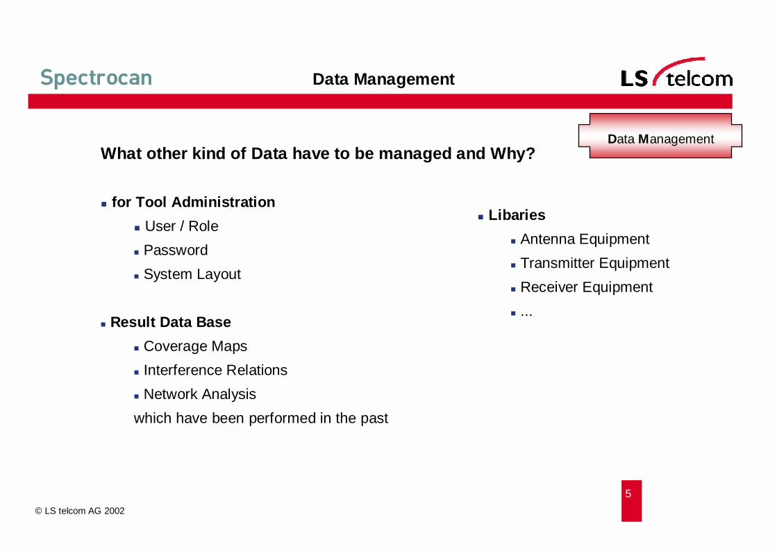
What other kind of Data have to be managed and Why?
� for Tool Administration� User / Role� Password � System Layout
� Result Data Base� Coverage Maps� Interference Relations� Network Analysiswhich have been performed in the past
� Libaries� Antenna Equipment� Transmitter Equipment� Receiver Equipment� ...

6
© LS telcom AG 2002
TxTx Power
Connector Loss
Branching Loss
Feeder Loss
Gain
EIRP
Rx
Feeder Loss
Branching Loss
Connector Loss
Gain
Receive Level
Pathloss
Site 1
Antenna
Device
OperatorSite 2
Data Management
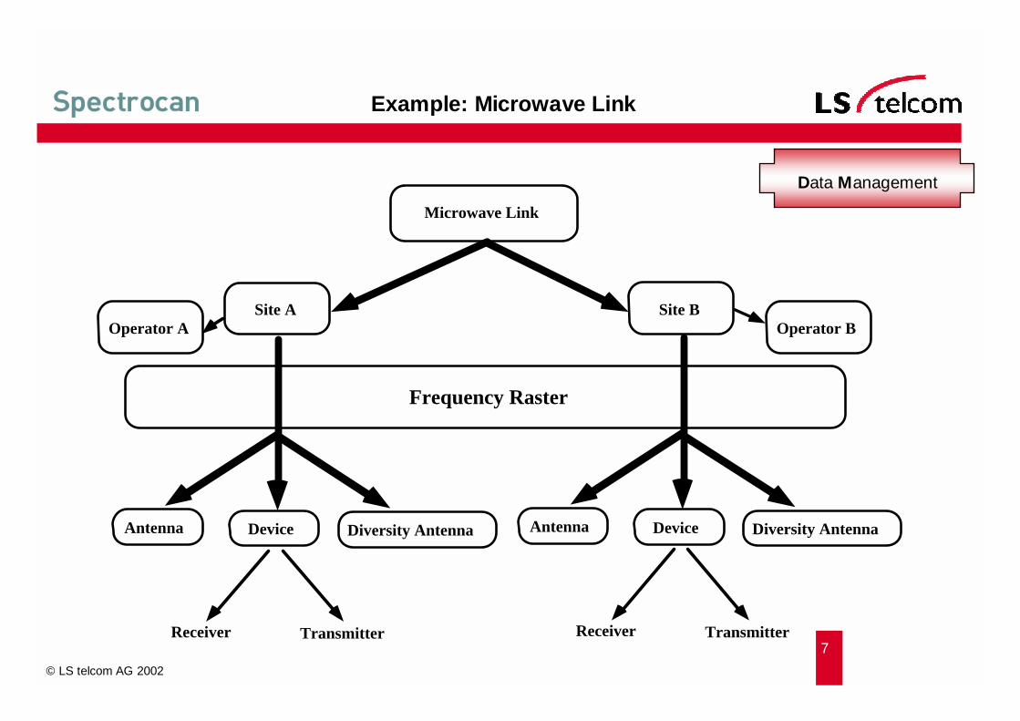
Example: Microwave Link
7
© LS telcom AG 2002
Microwave Link
Site A Site B
Frequency Raster
TransmitterReceiver
Antenna Diversity AntennaDevice
TransmitterReceiver
Antenna Diversity AntennaDevice
Operator A Operator B
Data Management
Example: Microwave Link

8
© LS telcom AG 2002
Work Database Work Database
Information Database
Client A Client B
Update IDB (area or project status) Update your WDB (area or project status)
Information Database
Central DB
Working Database
Data Management
Database Concepts

9
© LS telcom AG 2002
LivePlanning Tool Demonstration
10
© LS telcom AG 2002
Detailed Data Information� are necessary to perform comprehensive network analysis / optimisations
An comprehensive Data Management� allows keeping all network data in one central data base� makes daily work easier (Libraries)
Data Management

11
© LS telcom AG 2002
Modern Radio Network Planning Tools
Geo Information System
Data Management
Graphical User Interface
Propagation Prediction
Interference Analysis
Network Processor
Data / Result Output
Radio Network Planning ToolGraphical User Interface

12
© LS telcom AG 2002
Spreadsheets offer a view on database tables. All records of the related database table (e.g all sectors) can be edited:
Each column stands for one specific database field e.g Antenna Height
Each row contains information for one object e.g Antenna type, antenna height, azimuth etc. for a specific sector
The following options are available to work with spreadsheets� Edit functions� Query Functions� Functions to change the layout of the spreadsheet� Functions for graphical display of the spreadsheet data� Import / Export Functions
Spreadsheets
Graphical User Interface

13
© LS telcom AG 2002
Editor views allow to edit all data related to a specific object
Editors
Graphical User Interface

14
© LS telcom AG 2002
Menu
Toolbar
Working map
Value display (status bar)
Working Window
Graphical User Interface
15
© LS telcom AG 2002
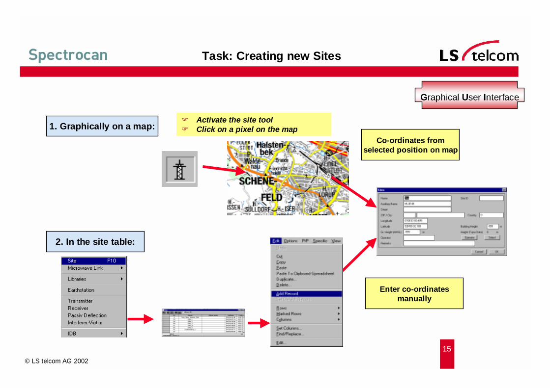
� Activate the site tool� Click on a pixel on the map1. Graphically on a map:
2. In the site table:
Co-ordinates fromselected position on map
Enter co-ordinatesmanually
Task: Creating new Sites
Graphical User Interface
16
© LS telcom AG 2002
LivePlanning Tool Demonstration

17
© LS telcom AG 2002
Modern Radio Network Planning Tools
Geo Information System
Data Management
Graphical User Interface
Propagation Prediction
Interference Analysis
Network Processor
Data / Result Output
Radio Network Planning ToolPropagation Prediction

18
© LS telcom AG 2002
diffraction
refraction
free space propagation
scattering reflection
tropospheric effects
Propagation Prediction
Wave Propagation Effects
Atmospheric Absorption Lossf>10 GHz
Rain Attenuationf>5GHz

19
© LS telcom AG 2002
θθθθ1
n1
n2
θθθθ2
Refraction
Propagation Prediction
0 4 8 12 16 20 24 28 32 36 40
Distance in km
Earth Radius
K= 4/3 StandardAtmosphere
K=1, homogene Atmosphere
Low density
High density
The refraction of the VHF/UHF signal in the troposphere causes an enhancement of the radio horizon compared to the geometric horizon

20
© LS telcom AG 2002
� replace obstacles by Knife-edges
Diffraction
Propagation PredictionDiffraction:
� a signal could be received even if there is no line of sight
� diffraction means also an attenuation of the wave.
� higher frequency -> higher diffraction attenuation.

21
© LS telcom AG 2002
θθθθi θθθθr
d1
εεεεr
d2Rd2T
d2 = d2T + d2R
d
( )221 TR hhdd −+=
( )222 TR hhdd ++=
hT hR
Reflection
Propagation Prediction

22
© LS telcom AG 2002
from volumefrom rough surfacefrom point
Ei
Es
Ei
Es
Ei Es
Scattering
analytical model for spherenumerical techniques
modified reflection coefficient radiative transfer theorystatistical models
Propagation Prediction
23
© LS telcom AG 2002
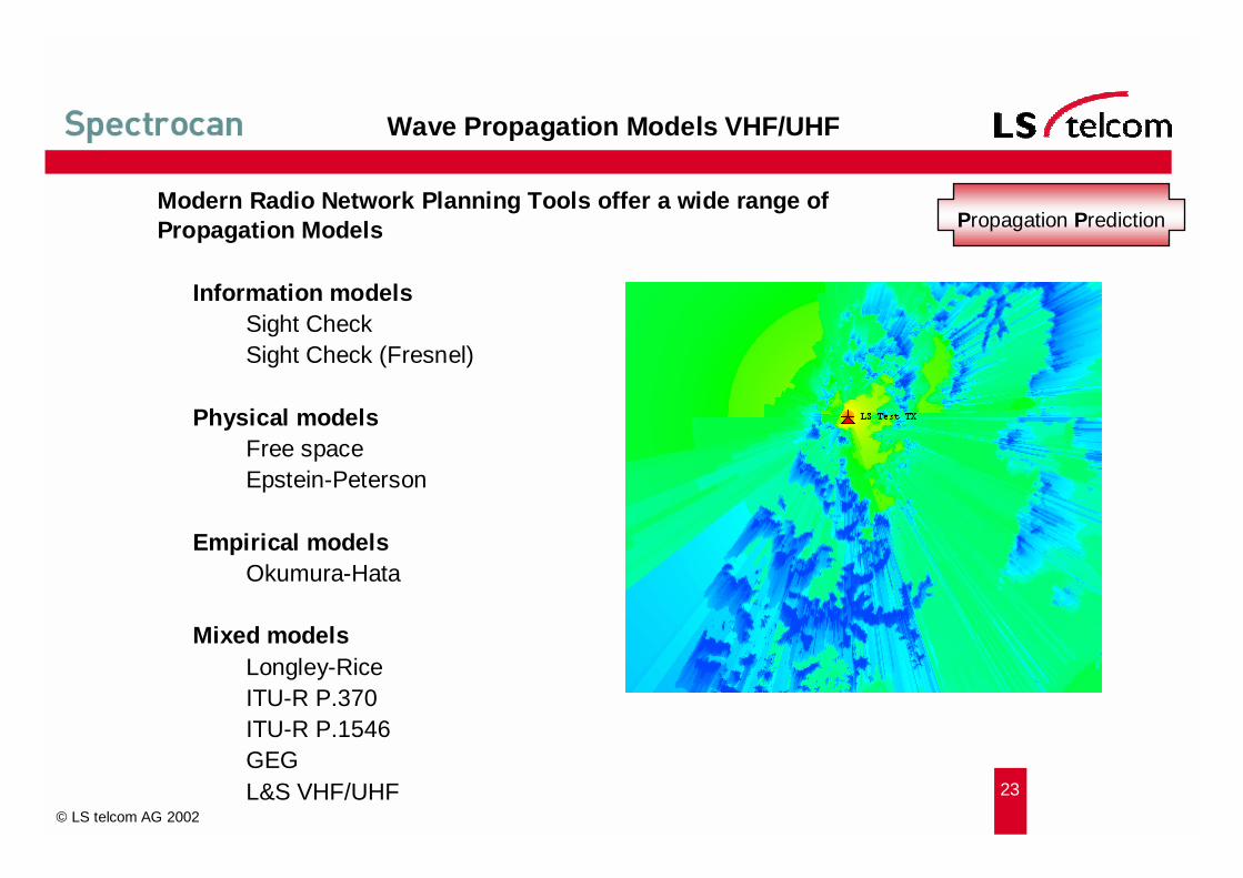
Information modelsSight CheckSight Check (Fresnel)
Physical modelsFree spaceEpstein-Peterson
Empirical modelsOkumura-Hata
Mixed modelsLongley-RiceITU-R P.370ITU-R P.1546GEGL&S VHF/UHF
Wave Propagation Models VHF/UHF
Propagation PredictionModern Radio Network Planning Tools offer a wide range of Propagation Models

24
© LS telcom AG 2002
30 Hz 300 Hz 30KHz 300 KHz 3 MHz 30 MHz 300 MHz 3 GHz 30 GHz 300 GHz
70GHz
2 GHz
1,7MHz
30 MHz
30MHz
10GHz
1GHz
1,5GHz
800MHz
1,5GHz
150MHz
30MHz
30MHz
3MHz
10 kHz
150kHz
Ground Wave Model
Sky Wave Model
Free Space Model
ITU533 Shortwave Model
Flat Earth Model
ITU370 Model
Okumura Hata Model 1
Okumura Hata Model 2
HCM Model
ITU452 Microwave Model
VLF LF MF HF VHF UHF SHF EHF3KHz
70GHz800MHzITU530 Microwave Model
Aeronautical Model
Egli Urban Model
CEPT Model
ITU 567 Model
Longley Rice Model
Walfish Ikegami Model
30GHz
10GHz30MHz
30MHz 250 MHz
30MHz 1 GHz
30MHz 40GHz
800MHz 2GHz
2GHz30MHz
30MHz
Version 15.05.2002 FF
Models and Frequency Ranges

25
© LS telcom AG 2002
performs line of sight (LOS) check
result sight
no sight
TX
profile
Propagation Prediction
Sight Check

26
© LS telcom AG 2002
performs extended line of sight (LOS) check
resultsight, no obstacles within 1st Fresnel zone
sight, but obstacle within 1st Fresnel zone
no sight
profile
TX
Propagation Prediction
Sight Check (Fresnel)

27
© LS telcom AG 2002
0
20
40
60
80
100
120
140
160
180
0 10 20 30 40 50 60 70 80 90 100d [km]
E [d
BuV/
m]
ERP = 1 WERP = 10 WERP = 100 WERP = 1 kW
propagation over a flat earth
Propagation Prediction
Free Space
� Determines the field strength value purely on the basis of the loss due to the distance d from the transmitter
� Selected calculation mode affects the k-factor for the calculation (see sight check)� Additionally the consideration of morphological classes is possible if available; the
clutter heights of the urban and rural morphologic classes are added to the topological heights

28
© LS telcom AG 2002Used for highest compatibility with international planning procedures
Propagation Prediction
Propagation Model ITU-R 370
latest version 1995coordination model ⇒ tends to overestimate fieldstrengthbasis:measured data from North America, Europe, North Sea (cold) and Mediterranean
Sea (warm)condensed to a set of curves: fieldstrength E over a homogenous terrain as a
function of distance d (10 km ... 1 000 km) for ...� frequency ranges VHF (30 ... 250 MHz) and UHF (450 ... 1 000 MHz)� power of 1kW ERP� effective transmitter antenna height 37.5 m ... 1 200 m (3 km ≤ d ≤ 15 km)� terrain roughness ∆h = 50 m (10 km ≤ d ≤ 50 km)� receiver location over land, cold sea or warm sea� receiver antenna height hR = 10 m� 50 % location probability� 1%, 5%, 10% and 50% time probability
29
© LS telcom AG 2002
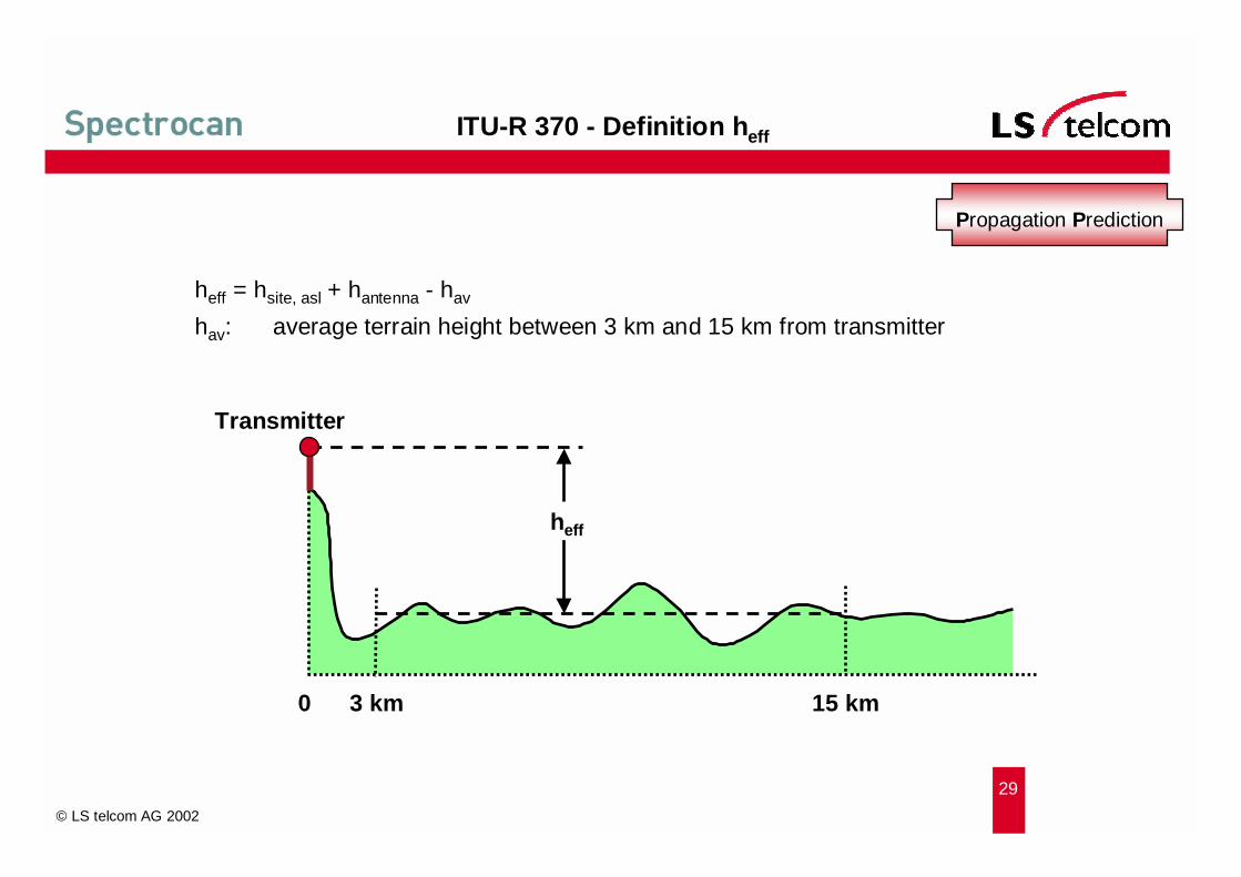
heff = hsite, asl + hantenna - hav
hav: average terrain height between 3 km and 15 km from transmitter
Transmitter
15 km0
heff
3 km
ITU-R 370 - Definition heff
Propagation Prediction
30
© LS telcom AG 2002
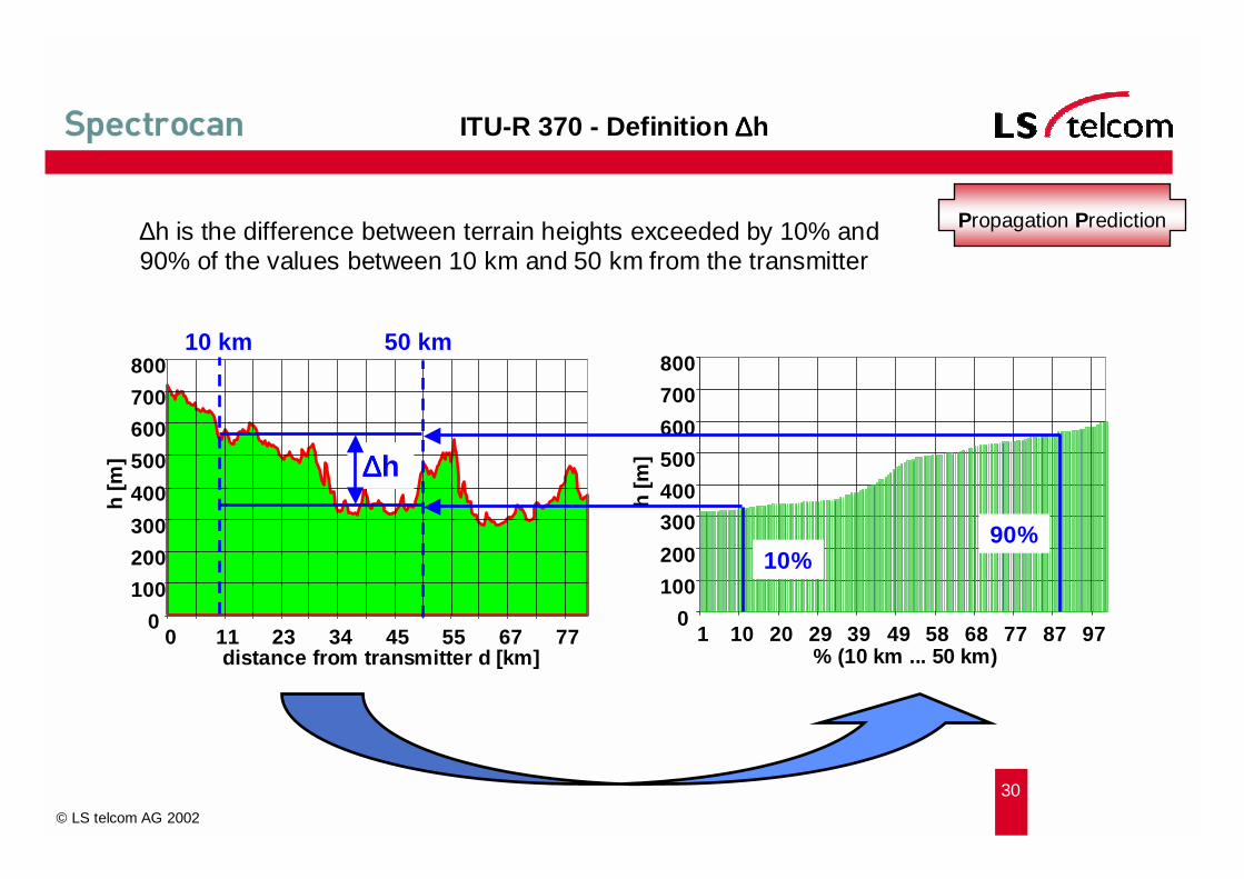
∆h is the difference between terrain heights exceeded by 10% and 90% of the values between 10 km and 50 km from the transmitter
0100200300400500600700800
0 11 23 34 45 55 67 77distance from transmitter d [km]
h [m
]
0100200300400500600700800
1 10 20 29 39 49 58 68 77 87 97% (10 km ... 50 km)
h [m
]∆∆∆∆h
10 km 50 km
10%90%
ITU-R 370 - Definition ∆∆∆∆h
Propagation Prediction

31
© LS telcom AG 2002
heff = 150 m
Free space propagationFree space propagation
heff = 150 m
propagation curve 50% time(steady or continuous)
propagation curve 1% time(tropospheric)
ITU-R 370 – Propagation Curves
Propagation Prediction

32
© LS telcom AG 2002
3 different Implementations for ITU-R 370 Models
ITU-R 370 Databaseeffective antenna height from database∆h = const. from user
ITU-R 370 Transmittereffective antenna height from database∆h dynamically from digital terrain data
ITU-R 370 Terraineffective antenna from digital terrain data∆h dynamically from digital terrain data
-> see Live Demo
Propagation Prediction
ITU-R 370 – Implementations

33
© LS telcom AG 2002
Major changes between ITU-R 370 and ITU-R 1546
� Interpolation and extension in frequency (between 3 curves from 30 MHz ... 3 000 MHz)
� Extension to distances below 10 km from transmitter (1 km)� Terrain roughness is no longer a parameter� More complex calculation near the transmitter� calculation procedure for negative heff, curves extended to 10 m� Interpolation for time variability (between curves)� Location's standard deviation as a function of frequency� More complex land sea path calculation
The New Model: ITU-R 1546
Propagation Prediction

34
© LS telcom AG 2002
� empirical model for propagation along flat and homogenous urban terrain� based on measurements for vertical polarization by Okumura and ...� interpolated formulas by Hata
� calculation of effective transmitter antenna height hT → hT,eff (different options)
� additional diffraction term for paths without sight� consideration of morphological heights in diffraction term� subdivision of the 4 morphological classes of Okumura-Hata into 16 classes
(morphological gain with respect to urban areas)� correction for non flat earth (terrain slope)
Extensions to Okumura-Hata
Okumura-Hata
Propagation Prediction

35
© LS telcom AG 2002
Edit coefficients ofhata equation
Edit coefficients ofhata equation
Set frequency and receiver heigth
Set frequency and receiver heigth
Enable earth curvaturecorrection
Enable earth curvaturecorrection
Enable diffraction model-Deygout (ITU)-Epsteint Petersen-Deygout (enhanced for speed)
Enable diffraction model-Deygout (ITU)-Epsteint Petersen-Deygout (enhanced for speed)
Edit parameter for tangent fitting
Edit parameter for tangent fitting
Select environment correction
Select environment correction
Set parameter for morphomodel
Set parameter for morphomodel
Select morphomodel
Select morphomodel
Model parameters for Extended Hata Model
Okumura-Hata
Propagation Prediction

36
© LS telcom AG 2002
Micro Cell Model
Propagation Prediction

37
© LS telcom AG 2002
• Use of "effective antenna height"• Monotonous decline of field strength withincreasing distance to transmitter
Example: ITU-R P. 370
Non-Terrain Based
DTM Based
• Diffraction, shading, reflection• Terrain elevation and land use (morphology)• 2D and 3D models
Examples: "Epstein-Peterson", "Longley&Rice", "Okumura-Hata"
Propagation Prediction
Prediction Models

38
© LS telcom AG 2002
LivePlanning Tool Demonstration