Embed Size (px)
Citation preview

R Package shape: functions for plotting graphical
shapes, colors...
Karline SoetaertRoyal Netherlands Institute of Sea Research
Yerseke, The Netherlands
Abstract
This document describes how to use the shape package for plotting graphical shapes.Together with R-package diagram (Soetaert 2009a) this package has been written to
produce the figures of the book (Soetaert and Herman 2009)
Keywords: graphics, shapes, colors, R.
1. Introduction
This vignette is the Sweave application of parts of demo colorshapes in package shape(Soetaert 2009b).
2. colors
Although one can find similar functions in other packages (including the R base package (RDevelopment Core Team 2008)), shape includes ways to generate color schemes;
• intpalette creates transitions between several colors;
• shadepalette creates a gradient between two colors, useful for shading (see below).
• drapecol drapes colors over a persp plot;
by default the red-blue-yellow (matlab-type) colors are used. The code below demonstratesthese functions (Figure 1)
> par(mfrow = c(2, 2))
> image(matrix(nrow = 1, ncol = 50, data = 1:50),
+ main = "intpalette",
+ col = intpalette(c("red", "blue", "yellow", "green", "black"),
+ numcol = 50))
> #
> shadepalette(n = 10, "white", "black")
[1] "#000000" "#1C1C1C" "#393939" "#555555" "#717171" "#8E8E8E" "#AAAAAA" "#C6C6C6"
[9] "#E3E3E3" "#FFFFFF"

2 R Package shape: functions for plotting graphical shapes, colors...
[1] "#000000" "#1C1C1C" "#393939" "#555555" "#717171" "#8E8E8E" "#AAAAAA" "#C6C6C6"
[9] "#E3E3E3" "#FFFFFF"
−1.0 −0.5 0.0 0.5 1.0
0.0
0.4
0.8
intpalette
−1.0 −0.5 0.0 0.5 1.0
0.0
0.4
0.8
shadepalette
volca
noYZ
drapecol
Figure 1: Use of intpalette, shadepalette and drapecol
> #
> image(matrix(nrow = 1, ncol = 50, data = 1:50),
+ col = shadepalette(50, "red", "blue"),
+ main = "shadepalette")
> #
> par(mar = c(0, 0, 0, 0))
> persp(volcano, theta = 135, phi = 30, col = drapecol(volcano),
+ main = "drapecol", border = NA)
3. Rotating
Function rotatexy rotates graphical shapes; it can be used to generate strangely-coloredshapes (Figure 2).

Karline Soetaert 3
> par(mfrow = c(2, 2), mar = c(3, 3, 3, 3))
> #
> # rotating points on a line
> #
> xy <- matrix(ncol = 2, data = c(1:5, rep(1, 5)))
> plot(xy, xlim = c(-6, 6), ylim = c(-6, 6), type = "b",
+ pch = 16, main = "rotatexy", col = 1)
> for (i in 1:5)
+ points(rotatexy(xy, mid = c(0, 0), angle = 60*i),
+ col = i+1, type = "b", pch = 16)
> points(0, 0, cex = 2, pch = 22, bg = "black")
> legend("topright", legend = 60*(0:5), col = 1:6, pch = 16,
+ title = "angle")
> legend("topleft", legend = "midpoint", pt.bg = "black",
+ pt.cex = 2, pch = 22, box.lty = 0)
> #
> # rotating lines..
> #
> x <- seq(0, 2*pi, pi/20)
> y <- sin(x)
> cols <- intpalette(c("blue", "green", "yellow", "red"), n = 125)
> cols <- c(cols, rev(cols))
> plot(x, y, type = "l", ylim = c(-3, 3), main = "rotatexy",
+ col = cols[1], lwd = 2, xlim = c(-1, 7))
> for (i in 2:250)
+ lines(rotatexy(cbind(x, y), angle = 0.72*i), col = cols[i], lwd = 2)
> #
> #
> x <- seq(0, 2*pi, pi/20)
> y <- sin(x*2)
> cols <- intpalette(c("red", "yellow", "black"), n = 125)
> cols <- c(cols, rev(cols))
> plot(x, y, type = "l", ylim = c(-4, 5), main = "rotatexy,
+ asp = TRUE", col = cols[1], lwd = 2, xlim = c(-1, 7))
> for (i in 2:250)
+ lines(rotatexy(cbind(x, y), angle = 0.72*i, asp = TRUE),
+ col = cols[i], lwd = 2)
> #
> # rotating points
> #
> cols <- femmecol(500)
> plot(x, y, xlim = c(-1, 1), ylim = c(-1, 1), main = "rotatexy",
+ col = cols[1], type = "n")
> for (i in 2:500) {
+ xy <- rotatexy(c(0, 1), angle = 0.72*i, mid = c(0, 0))
+ points(xy[1], xy[2], col = cols[i], pch = ".", cex = 2)
+ }

4 R Package shape: functions for plotting graphical shapes, colors...
● ● ● ● ●
−6 −4 −2 0 2 4 6
−6
−4
−2
02
46
rotatexy
xy[,1]
xy[,2
] ●
●
●
●
●
●
●
●
●
●
●●●●●●
●
●
●
●
●
●
●
●
●
●
●
●
●
●
●
angle
060120180240300
midpoint
0 2 4 6
−3
−2
−1
01
23
rotatexy
xy
0 2 4 6
−4
−2
02
4
rotatexy, asp = TRUE
y
−1.0 −0.5 0.0 0.5 1.0
−1.
0−
0.5
0.0
0.5
1.0
rotatexyy
Figure 2: Four examples of rotatexy
>
4. ellipses
If a suitable shading color is used, function filledellipse creates spheres, ellipses, donutswith 3-D appearance (Figure 3).
> par(mfrow = c(2, 2), mar = c(2, 2, 2, 2))
> emptyplot(c(-1, 1))
> col <- c(rev(greycol(n = 30)), greycol(30))
> filledellipse(rx1 = 1, rx2 = 0.5, dr = 0.1, col = col)
> title("filledellipse")
> #
> emptyplot(c(-1, 1), c(-1, 1))
> filledellipse(col = col, dr = 0.1)
> title("filledellipse")

Karline Soetaert 5
filledellipse filledellipse
filledellipse getellipse
Figure 3: Use of filledellipse, and getellipse
> #
> color <-gray(seq(1, 0.3, length.out = 30))
> emptyplot(xlim = c(-2, 2), ylim = c(-2, 2), col = color[length(color)])
> filledellipse(rx1 = 2, ry1 = 0.4, col = color, angle = 45, dr = 0.1)
> filledellipse(rx1 = 2, ry1 = 0.4, col = color, angle = -45, dr = 0.1)
> filledellipse(rx1 = 2, ry1 = 0.4, col = color, angle = 0, dr = 0.1)
> filledellipse(rx1 = 2, ry1 = 0.4, col = color, angle = 90, dr = 0.1)
> title("filledellipse")
> #
> emptyplot(main = "getellipse")
> col <-femmecol(90)
> for (i in seq(0, 180, by = 2))
+ lines(getellipse(0.5, 0.25, mid = c(0.5, 0.5), angle = i, dr = 0.1),
+ type = "l", col = col[(i/2)+1], lwd = 2)

6 R Package shape: functions for plotting graphical shapes, colors...
5. Cylinders, rectangles, multigonals
The code below draws cylinders, rectangles and multigonals (Figure 4).
> par(mfrow = c(2, 2), mar = c(2, 2, 2, 2))
> #
> # simple cylinders
> emptyplot(c(-1.2, 1.2), c(-1, 1), main = "filledcylinder")
> col <- c(rev(greycol(n = 20)), greycol(n = 20))
> col2 <- shadepalette("red", "blue", n = 20)
> col3 <- shadepalette("yellow", "black", n = 20)
> filledcylinder(rx = 0., ry = 0.2, len = 0.25, angle = 0,
+ col = col, mid = c(-1, 0), dr = 0.1)
> filledcylinder(rx = 0.0, ry = 0.2, angle = 90, col = col,
+ mid = c(-0.5, 0), dr = 0.1)
> filledcylinder(rx = 0.1, ry = 0.2, angle = 90, col = c(col2, rev(col2)),
+ mid = c(0.45, 0), topcol = col2[10], dr = 0.1)
> filledcylinder(rx = 0.05, ry = 0.2, angle = 90, col = c(col3, rev(col3)),
+ mid = c(0.9, 0), topcol = col3[10], dr = 0.1)
> filledcylinder(rx = 0.1, ry = 0.2, angle = 90, col = "white",
+ lcol = "black", lcolint = "grey", dr = 0.1)
> #
> # more complex cylinders
> emptyplot(c(-1, 1), c(-1, 1), main = "filledcylinder")
> col <- shadepalette("blue", "black", n = 20)
> col2 <- shadepalette("red", "black", n = 20)
> col3 <- shadepalette("yellow", "black", n = 20)
> filledcylinder(rx = 0.025, ry = 0.2, angle = 90,
+ col = c(col2, rev(col2)), dr = 0.1, mid = c(-0.8, 0),
+ topcol = col2[10], delt = -1., lcol = "black")
> filledcylinder(rx = 0.1, ry = 0.2, angle = 00,
+ col = c(col, rev(col)), dr = 0.1, mid = c(0.0, 0.0),
+ topcol = col, delt = -1.2, lcol = "black")
> filledcylinder(rx = 0.075, ry = 0.2, angle = 90,
+ col = c(col3, rev(col3)), dr = 0.1, mid = c(0.8, 0),
+ topcol = col3[10], delt = 0.0, lcol = "black")
> #
> # rectangles
> color <- shadepalette(grey(0.3), "blue", n = 20)
> emptyplot(c(-1, 1), main = "filledrectangle")
> filledrectangle(wx = 0.5, wy = 0.5, col = color,
+ mid = c(0, 0), angle = 0)
> filledrectangle(wx = 0.5, wy = 0.5, col = color,
+ mid = c(0.5, 0.5), angle = 90)
> filledrectangle(wx = 0.5, wy = 0.5, col = color,
+ mid = c(-0.5, -0.5), angle = -90)
> filledrectangle(wx = 0.5, wy = 0.5, col = color,

Karline Soetaert 7
+ mid = c(0.5, -0.5), angle = 180)
> filledrectangle(wx = 0.5, wy = 0.5, col = color,
+ mid = c(-0.5, 0.5), angle = 270)
> #
> # multigonal
> color <- shadepalette(grey(0.3), "blue", n = 20)
> emptyplot(c(-1, 1))
> filledmultigonal(rx = 0.25, ry = 0.25,
+ col = shadepalette(grey(0.3), "blue", n = 20),
+ nr = 3, mid = c(0, 0), angle = 0)
> filledmultigonal(rx = 0.25, ry = 0.25,
+ col = shadepalette(grey(0.3), "darkgreen", n = 20),
+ nr = 4, mid = c(0.5, 0.5), angle = 90)
> filledmultigonal(rx = 0.25, ry = 0.25,
+ col = shadepalette(grey(0.3), "orange", n = 20),
+ nr = 5, mid = c(-0.5, -0.5), angle = -90)
> filledmultigonal(rx = 0.25, ry = 0.25, col = "black",
+ nr = 6, mid = c(0.5, -0.5), angle = 180)
> filledmultigonal(rx = 0.25, ry = 0.25, col = "white", lcol = "black",
+ nr = 7, mid = c(-0.5, 0.5), angle = 270)
> title("filledmultigonal")
>
6. Other shapes
Function filledshape is the most flexible drawing function from shape: just specify an innerand outer shape and fill with a color scheme (Figure 5).
> par(mfrow = c(2, 2), mar = c(2, 2, 2, 2))
> #an egg
> color <- greycol(30)
> emptyplot(c(-3.2, 3.2), col = color[length(color)],
+ main = "filledshape")
> b <- 4
> a <- 9
> x <- seq(-sqrt(a), sqrt(a), by = 0.1)
> g <- b-b/a*x^2-0.2*b*x+0.2*b/a*x^3
> g[g<0] <- 0
> x1 <- c(x, rev(x))
> g1 <- c(sqrt(g), rev(-sqrt(g)))
> xouter <- cbind(x1, g1)
> xouter <- rbind(xouter, xouter[1, ])
> filledshape(xouter, xyinner = c(-1, 0), col = color)
> #
> # a mill
> color <- shadepalette(grey(0.3), "yellow", n = 20)

8 R Package shape: functions for plotting graphical shapes, colors...
filledcylinder filledcylinder
filledrectangle filledmultigonal
Figure 4: Use of filledcylinder, filledrectangle and filledmultigonal

Karline Soetaert 9
> emptyplot(c(-3.3, 3.3), col = color[length(color)],
+ main = "filledshape")
> x <- seq(0, 0.8*pi, pi/20)
> y <- sin(x)
> xouter <- cbind(x, y)
> for (i in seq(0, 360, 60))
+ xouter <- rbind(xouter,
+ rotatexy(cbind(x, y), mid = c(0, 0), angle = i))
> filledshape(xouter, c(0, 0), col = color)
> #
> # abstract art
> emptyplot(col = "darkgrey", main = "filledshape")
> filledshape(matrix(nc = 2, runif(80)), col = "darkblue")
> #
> emptyplot(col = "darkgrey", main = "filledshape")
> filledshape(matrix(nc = 2, runif(80)),
+ col = shadepalette(20, "darkred", "darkblue"))
7. arrows, arrowheads
As the arrow heads in the R base package are too simple for some applications, there aresome improved arrow heads in shape (Figure 6).
> par(mfrow = c(2, 2), mar = c(2, 2, 2, 2))
> xlim <- c(-5 , 5)
> ylim <- c(-10, 10)
> x0<-runif(100, xlim[1], xlim[2])
> y0<-runif(100, ylim[1], ylim[2])
> x1<-x0+runif(100, -2, 2)
> y1<-y0+runif(100, -2, 2)
> size <- 0.4
> plot(0, type = "n", xlim = xlim, ylim = ylim)
> Arrows(x0, y0, x1, y1, arr.length = size, arr.type = "triangle",
+ arr.col = rainbow(runif(100, 1, 20)))
> title("Arrows")
> #
> # arrow heads
> #
> ang <- runif(100, -360, 360)
> plot(0, type = "n", xlim = xlim, ylim = ylim)
> Arrowhead(x0, y0, ang, arr.length = size, arr.type = "curved",
+ arr.col = rainbow(runif(100, 1, 20)))
> title("Arrowhead")
> #
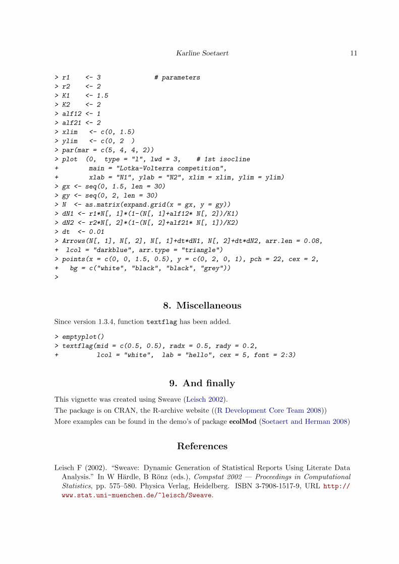
> # Lotka-Volterra competition model
> #

10 R Package shape: functions for plotting graphical shapes, colors...
filledshape filledshape
filledshape filledshape
Figure 5: Use of filledshape
Karline Soetaert 11
> r1 <- 3 # parameters
> r2 <- 2
> K1 <- 1.5
> K2 <- 2
> alf12 <- 1
> alf21 <- 2
> xlim <- c(0, 1.5)
> ylim <- c(0, 2 )
> par(mar = c(5, 4, 4, 2))
> plot (0, type = "l", lwd = 3, # 1st isocline
+ main = "Lotka-Volterra competition",
+ xlab = "N1", ylab = "N2", xlim = xlim, ylim = ylim)
> gx <- seq(0, 1.5, len = 30)
> gy <- seq(0, 2, len = 30)
> N <- as.matrix(expand.grid(x = gx, y = gy))
> dN1 <- r1*N[, 1]*(1-(N[, 1]+alf12* N[, 2])/K1)
> dN2 <- r2*N[, 2]*(1-(N[, 2]+alf21* N[, 1])/K2)
> dt <- 0.01
> Arrows(N[, 1], N[, 2], N[, 1]+dt*dN1, N[, 2]+dt*dN2, arr.len = 0.08,
+ lcol = "darkblue", arr.type = "triangle")
> points(x = c(0, 0, 1.5, 0.5), y = c(0, 2, 0, 1), pch = 22, cex = 2,
+ bg = c("white", "black", "black", "grey"))
>
8. Miscellaneous
Since version 1.3.4, function textflag has been added.
> emptyplot()
> textflag(mid = c(0.5, 0.5), radx = 0.5, rady = 0.2,
+ lcol = "white", lab = "hello", cex = 5, font = 2:3)
9. And finally
This vignette was created using Sweave (Leisch 2002).
The package is on CRAN, the R-archive website ((R Development Core Team 2008))
More examples can be found in the demo’s of package ecolMod (Soetaert and Herman 2008)
References
Leisch F (2002). “Sweave: Dynamic Generation of Statistical Reports Using Literate DataAnalysis.” In W Hardle, B Ronz (eds.), Compstat 2002 — Proceedings in ComputationalStatistics, pp. 575–580. Physica Verlag, Heidelberg. ISBN 3-7908-1517-9, URL http://
www.stat.uni-muenchen.de/~leisch/Sweave.

12 R Package shape: functions for plotting graphical shapes, colors...
−4 −2 0 2 4
−10
−5
05
10
Index
Arrows
−4 −2 0 2 4
−10
−5
05
10
Index
0
Arrowhead
0.0 0.5 1.0 1.5
0.0
0.5
1.0
1.5
2.0
Lotka−Volterra competition
N1
N2
Figure 6: Use of Arrows and Arrowhead

Karline Soetaert 13
hello
Figure 7: Use of function textflag
R Development Core Team (2008). R: A Language and Environment for Statistical Computing.R Foundation for Statistical Computing, Vienna, Austria. ISBN 3-900051-07-0, URL http:
//www.R-project.org.
Soetaert K (2009a). diagram: Functions for visualising simple graphs (networks), plottingflow diagrams. R package version 1.4.
Soetaert K (2009b). shape: Functions for plotting graphical shapes, colors. R package version1.2.2.
Soetaert K, Herman PM (2008). ecolMod: ”A practical guide to ecological modelling - usingR as a simulation platform”. R package version 1.1.
Soetaert K, Herman PMJ (2009). A Practical Guide to Ecological Modelling. Using R as aSimulation Platform. Springer. ISBN 978-1-4020-8623-6.
Affiliation:
Karline SoetaertRoyal Netherlands Institute of Sea Research (NIOZ)4401 NT Yerseke, Netherlands E-mail: [email protected]: http://www.nioz.nl