THE RELATIONSHIP BETWEEN INFLATION RATES AND REAL

ESTATE PRICES IN KENYA. CASE OF NAIROBI COUNTY

BY

SYLVIA KANGOGO C.

D61/66842/2011

A RESEARCH PROJECT SUMMITTED TO THE DEPARTMENT OF

FINANCE AND ACCOUNTING IN PARTIAL FULFILMENT OF THE

REQUIREMENT FOR THE DEGREE OF MASTER OF BUSINESS

ADMINISTRATION, UNIVERSITY OF NAIROBI.

OCTOBER 2013

ii

DECLARATION

I declare that this research project is my original work and has not been presented for a

degree in any other university.

Signed______________________ Date______________________

Sylvia Kangogo C.

D61/66842/2011

This research project has been presented for examination with my approval as the

university supervisor.

Signed______________________ Date_______________________

Dr. Josiah O. Aduda

Chairman Department of Finance and Accounting.

School of business

University of Nairobi

iii

ACKNOWLEDGEMENT

First and for most I would like to acknowledge the almighty God for enabling me to carry

out my studies and giving me the strength and finance to complete them.

The successful completion of this project would have not been possible without the

support of several people. To my supervisor Dr. J. Aduda for your dedicated support and

guidance that led to the completion of this project. Thank you.

I thank all the lecturers and colleagues from the university as well as the staff of the

ministry of Lands, Housing and Urban development, Kenya National Bureau of statistics

and all who contributed to my completion of this project. Thank you.

I thank my parents and family for their unwavering support, my mother for instilling the

hard work character in me that has led to a successful completion this project. To my

husband and children your support and time you gave me is unmmeasurable. God bless

you all.

iv

DEDICATION

I dedicate this project to my parents, siblings, my husband Isaac and children Alvin and

Mitchelle.

v

TABLE OF CONTENTS DECLARATION............................................................................................................... ii

ACKNOWLEDGEMENT ............................................................................................... iii

DEDICATION.................................................................................................................. iv

LIST OF TABLES ......................................................................................................... viii

LIST OF FIGURES ABSTRACT .................................................................................. ix

ABSTRACT ....................................................................................................................... x

ABBREVIATIONS .......................................................................................................... xi

CHAPTER ONE ............................................................................................................... 1

1.0 Introduction ................................................................................................................... 1

1.1 Background of the Study .............................................................................................. 1

1.1.1 Inflation .................................................................................................................. 3

1.1.2 Types of Inflation ................................................................................................... 5

1.1.2.1 Creeping Inflation ............................................................................................ 5

1.1.2.2 Galloping Inflation .......................................................................................... 5

1.1.2.3 Hyperinflation .................................................................................................. 5

1.1.2.4 Stagflation ........................................................................................................ 6

1.1.3 Property Prices ....................................................................................................... 6

1.1.4 Real Estate Market ................................................................................................. 8

1.2 Statement of the Problem .............................................................................................. 9

1.3 Objectives of the Study ............................................................................................... 10

1.4 Significance of the Study ............................................................................................ 10

1.4.1 Investors ............................................................................................................... 10

1.4.2 Scholars and Researchers ..................................................................................... 11

1.4.3 Financial institutions ............................................................................................ 11

1.4.4 The Government ................................................................................................... 11

1.4.5 Agents and Brokers .............................................................................................. 12

vi

CHAPTER TWO ............................................................................................................ 13

2.0 Literature review ......................................................................................................... 13

2.1 Introduction ................................................................................................................. 13

2.2 Review of Theories ..................................................................................................... 13

2.2.1 Prospect Theory.................................................................................................... 13

2.2.2 Efficient Market Hypothesis (EMH) .................................................................... 14

2.2.3 Rational Expectation Theory ................................................................................ 15

2.2.4 Dynamic Gordon Growth Model Theory ............................................................. 16

2.2.5 The Gordon Growth Model Theory ..................................................................... 17

2.2.6 Monetarism Theory of Inflation ........................................................................... 17

2.3 Empirical Evidence ..................................................................................................... 18

2.4 Conclusion of Literature Review ................................................................................ 21

CHAPTER THREE ........................................................................................................ 22

3.0 Research Methodology ............................................................................................... 22

3.1 Introduction ................................................................................................................. 22

3.2 Research Design.......................................................................................................... 22

3.3 Population ................................................................................................................... 22

3.4 Sample and sampling Technique ................................................................................ 23

3.5 Data collection ............................................................................................................ 23

3.6 Data analysis. .............................................................................................................. 23

CHAPTER FOUR ........................................................................................................... 25

4.0 Data Analysis and Presentation of the Findings. ........................................................ 25

4.1 Introduction ................................................................................................................. 25

4.2 Data presentation ........................................................................................................ 25

4.3 Summary and interpretation of the findings ............................................................... 29

4.4 Summary of the study ................................................................................................. 32

vii

CHAPTER FIVE ............................................................................................................ 34

5.0 Summary, Conclusion and Recomentations ............................................................... 34

5.1 Summary ..................................................................................................................... 34

5.2 Conclusion .................................................................................................................. 35

5.3 Policy recommendations. ............................................................................................ 35

5.4 Limitation o the study. ................................................................................................ 36

5.5 Suggestions for further studies.................................................................................... 37

REFFERENCES ............................................................................................................. 38

APPENDICES ................................................................................................................. 42

Appendix 1: Property Price And Inflation Rate For Kileleswa, Lavington And Kilimani

........................................................................................................................................... 42

Appendix II: Quarterly prices and Inflation Rates For Kileleswa,Lavington and Kilimani

........................................................................................................................................... 45

Appendix III: Property prices and inflation rates for embakasi, kasarani, buruburu, and

Mombasa road south B & C....................................................................... 44

Appendix IV: Quarterly Prices and Inflation Rates Embakasi, Kasarani,Buruburu and

Mombasa Road ( South B & C) ............................................................... 47

Appendix V: Regression output for Kileleswa, Lavington and Kilimani ......................... 50

Appendix VI: Regression output for Embakasi, Buruburu, Kasarani and Mombasa road

South B & C ............................................................................................ 55

viii

LIST OF TABLES

Table 4.1: Property price and inflation rates for Kileleswa, Lavington and Kilimani...... 25

Table 4.2: For Property price and inflation rates for Embakasi, Kasarani, Buruburu and

South B & C ...................................................................................................... 26

Table 4.3 Quarterly property prices and inflation rates for Kileleswa, Lavington and 28

Kilimani. ............................................................................................................ 28

Table 4.4 Quarterly property price and inflation rates for Embakasi, Buruburu, Kasarani

and South B & C. Quarterly data. ...................................................................... 29

ix

LIST OF FIGURES

Figure 4.1: Data Analysis for Kileleswa, Lavington and Kilimani ................................. 30

Figure 4.2 Property prices and inflation movement .......................................................... 31

x

ABSTRACT Real estate industry has been one of the most resilient, vibrant and profitable in the world

today. The growth has mainly been driven by urbanization, a strong economy and stable

legal environment, significant credit expansion and increased spending on infrastructure

by the government. Fluctuation in property prices have been experienced in many

countries, this is attributed to the financial instability result from the house price boom

and bust. According to the Kenya National Bureau of statistics, in Kenya the real estate

has been a driver of growth in the past five years. Real estate markets are continuously

adjusting to equilibrium where price range is adjusted according to variation in supply

influenced by changes national and regional economies. Inflation has pushed up the cost

of doing business contributing to the cutting down to the number of properties.

This project objective is to investigate the relationship between property price and the

inflation rates. The causal research design was used in this study and secondary data

which was analyzed using SPSS package. From the findings it was observed that there is

no clear defined relationship between the property prices and inflation rates. From the

analysis of variance (ANOVA) statistic the study shows that the processed data has the

significant level. This indicates that the data is ideal for making conclusion and it also

shows that the data sampled represent the population. We can observe that the regression

sum of squares is very huge implying that much of the variability is actually accounted

for in this regression model.

The p-value=0.000<0.05 (significance level) indicating that the model is appropriate and

significant. It can also be observed that property prices has been on a continuous increase

over the years but gradually while inflation rate rose sharply to its peak (double digit

)highest of 19.72% in the last quarter of 2012. It has been fluctuating to extreme

variations. The findings of this study shows that there is no clear relationship between

the property price and the inflation rate

xi

ABBREVIATIONS

DCF - Discounted Cash Flow

EMH - Efficient Market Hypothesis

GGM - Gordon Growth Model

TVM - Time Value of Money

KSH- Kenya Shilling

KNBS - Kenya Bureau of Statistics

NVP - Net Present Value

SPSS- Statistical package for social sciences

1

CHAPTER ONE

1.0 INTRODUCTION

1.1 Background of the Study

Inflation is described as the general rise in prices of goods and services and its felt by all

parties in the economy. It’s the reduction of buyers’ purchasing power and hence sellers

have to increase their prices in order to make profit, an increase in expected rate of

inflation causes an immediate increase in the value of real asset (Syagga, 1994). This

study wants to find out how the fluctuation in property price relates with the inflation.

Real estate sector is one of the most resilient, vibrant and profitable in the world today. In

Kenya it has been anything but robust. The growth has mainly been driven by

urbanization, a strong economic and growing middle-class, stable legal environment,

significant credit expansion and increased spending on infrastructure by the government

(Ojijo, 2011).

The real estate boom survived the 2008 post election violence and global economic

downturns that crippled other sectors such as tourism and agriculture in the country. The

market faced difficulties in 2011 due to weakening of the shilling against major

currencies, double digit inflation, and interest rates hike is taking its toll on real estate

industry. Developers and buyers are struggling to meet financing cost occasioned by high

interest rates triggered by aggressive tightening of monetary policy to counter the

weakening of the shilling (Waweru, 2011).

Real estate is the property consisting of land and buildings on it, along with its natural

resources such as crops, mineral water immovable property of this nature, an interest

2

vested in this, an item of real property, building or housing in general. It can also be

defined as the business of real estate, the profession of buying and selling or renting land,

building or housing. With the development of private property ownership, real estate has

become a major area of business. Commonly referred to as commercial real estate.

Purchasing real estate is a significant investment and each parcel of land has unique

characteristics so the real estate industry has evolved into several distinct fields.

Specialists are often called to value the real estate and facilitate transaction.

Real estate valuation is estimating the value of real property. It’s important in real estate

financing, listing real estate for sale, investment analysis property insurance and taxation

of real estate to know the worth of the property. Determining the asking or purchase price

of a property is the useful application of real estate valuation, value is not necessarily

equal to price. Price is the amount paid for a property, Johnson et al (2000). The basic

concepts of valuation are value, cost and price. According to Richmond (1994) market

value is the most probable price that the property will bring in a competitive and open

market. Market price is the price at which the property actually sells it may not always

represent the market value that is if the property was sold in private sale without being

exposed to the open market, the property will sale below its market value. Value is the

present worth of future benefits arising from the ownership of real property the benefits

are realized over a long period of time therefore estimating a property’s value must be

taken into considerations economic and social trends as well as governmental control or

regulations and environmental conditions, this may influence this element of value i.e.

demand, utility, scarcity and transferability.

3

Fluctuation in the property prices have been experience in many countries, this is

attributed to the financial instability resulting from the house price boom and bust.

According to Kenya National Bureau of statistic, in Kenya the real estate sector has been

a driver of growth in the past five years. Inflation has pushed up the cost of doing

business contributing to the cutting down of the number of properties. Investors in real

estate who are looking for safe haven for their money in turbulent times in the equity

markets have underestimated risk, property price fluctuations have been witnessed in

many countries over the past decades which have been associated with financial

instability. The resent financial crisis has led to the accelerated housing defaults in the

U.S and other countries (Burnside et al, 2011).

1.1.1 Inflation

Inflation is the rise in the general level of price of goods and services in an economy over

a period of time. It’s referred to the broad price index representing the overall price level

for goods and services in the economy. Inflation reflects a reduction in the purchasing

power per unit of money. Brown and Matysiak (2000). Inflation affects the property

value in that low inflation means low or no property values. It’s related to capital growth,

the real benefit from the capital growth is maintaining a hedge against inflation and over

and above it by increasing purchasing power of capital ahead of the rate of inflation,

(Fama and Gibbons 1982).

4

According to Brown and Matysiak (2000), inflation arises from some initiating influences

on demand and supply side that can be seen to contribute to the development of an

inflationary economy. That is if the demand for the property exceeds supply then the

asking price will be bid up. In real estate inflation has the effect of increasing the

monitory value of the future earnings which will in turn be reflected in capital values.

Price inflation has immense effect in TVM, this act as principal component of the real

rates of interest which forms the basis of all TVM calculation. According to KNBS

inflation has contributed to the slowing down of real estate market construction cost have

rise to 40%, currency. KSH has depreciated by 28% and inflation went up to 16.67%.

The cost of borrowing has also gone up and financial companies adjust their base lending

rates to reflect the weakening shilling. The rising lending rates will have a negative effect

on real estate sector by making mortgage unattractive for both existing and potential

clients.

The impact of inflation on the value of assets is considered one of the primary financial

concerns of long-term investors such as pension funds and life insurance companies since

the mid 1970s. Combating inflation has been the overriding goal of the Federal Reserve’s

monetary policy. The increase in the rate of inflation is still a dominant consideration for

long-term investors (Hartzell et al, 1978).

According to Rajesh Goyal an economic analyst inflation has been classified in two as

follows: first demand-pull inflation in this type of inflation prices increase results from an

excess of demand over supply for the economy as a whole demand inflation occurs when

supply cannot expand any more to meet demand; that is, when critical production factors

5

are being fully utilized, also called Demand inflation. The second is cost-push inflation.

This type of inflation occurs when general price levels rise owing to rising input costs. In

general, there are three factors that could contribute to Cost-Push inflation: rising wages

increases in corporate taxes, and imported inflation. Imported raw or partly-finished

goods may become expensive due to rise in international costs or as a result

of depreciation of local currency.

1.1.2 Types of Inflation

1.1.2.1 Creeping Inflation

This is also known as mild inflation or moderate inflation. This type of inflation occurs

when the price level persistently rises over a period of time at a mild rate. When the rate

of inflation is less than 10 per cent annually, or it is a single digit inflation rate, it is

considered to be a moderate inflation.

1.1.2.2 Galloping Inflation

If mild inflation is not checked and if it is uncontrollable, it may assume the character of

galloping inflation. Inflation in the double or triple digit range of 20, 100 or 200 percent a

year is called galloping inflation. Many Latin American countries such as Argentina,

Brazil had inflation rates of 50 to 700 percent per year in the 1970s and 1980s.

1.1.2.3 Hyperinflation

It is a stage of very high rate of inflation. While economies seem to survive under

galloping inflation, a third and deadly strain takes hold when the cancer of hyperinflation

strikes. Nothing good can be said about a market economy in which prices are rising a

6

million or even a trillion percent per year. Hyperinflation occurs when the prices go out

of control and the monetary authorities are unable to impose any check on it. Germany

had witnessed hyperinflation in 1920’s.

1.1.2.4 Stagflation

It is an economic situation in which inflation and economic stagnation or recession occur

simultaneously and remain unchecked for a period of time. Stagflation was witnessed by

developed countries in 1970s, when world oil prices rose dramatically.

1.1.3 Property Prices

Theoretically prices are assumed to develop within neo-classical economic structures in

which the core concept is demand and supply, market forces and equilibrium prices. Price

assert that the market reflects interaction between two opposing consideration. Demand

consideration based on utility and supply consideration based on marginal cost on the

other side. An equilibrium price is supposed to be at once equal to marginal utility from

the buyer’s side and marginal cost from the sellers’ side ( Sharpe, 1999)

Property prices have been the main focal point in the economic and social debate in the

developed countries. In Kenya it has been one of the most striking issues in the economy.

There are many factors affecting house price, this are mortgage, inflation etc. price is

assumed to developed within a neo-classical economic structure in which the core

concepts are supply and demand, market forces and equilibrium prices (Syagga, 1994)

Real estate markets are characterized by predictable cycle boom and bust. During the

cycle of booms the prices in the market sky rocket and almost inevitably, this season in

7

followed by busts (very low price). Prices in most areas are influenced by demand and

supply forces, are also limited by various factors such as the income of potential buyers,

the cost and the ability to construct new property to increase supply and demand. Access

of finance, ability to make payments and the cost of borrowing money has led to spiraling

cost of housing and escalating property prices.

Hass property has been tracking property prices in the upper and middle section of the

Kenya property market and has seen the average price in this sector rise. Property value

in the country have increased by 3.36 times since 2000 as the average value of property

rose from 7.1 millions in the year 2000 to 24.1 millions in 2012 according to their annual

housing report, (Hassconsult 2012).This rapid growth in real estate prices makes it

necessary for Kenyans to open up for mortgage credit. Property cost rise due to the rate

of construction of new property increase because investors, developers and speculators

are constantly monitoring the investment equation. They are also looking at the land

costs, when values are rising strongly then prospective profit are significantly enhanced,

when there is surplus of property in the market, values tend to level off and with inflation

real value will fall, Fred & Brett (1997). Mocoloo as cited in Muli (2011) examining the

building cost in Kenya which he found out that the high building cost had an impact on

the house prices has developers’ tries to maintain their profit taking opportunities.

Therefore for Kenyans to afford the highly priced property they need more financing

from the mortgage lenders.

8

1.1.4 Real Estate Market

Real estate markets are a combination of a regional and National economic and therefore

influenced by changes in these economies. Chin (2002) suggested that real estate markets

are continuously adjusting to equilibrium were price range is adjusted according to

variation in supply influenced by changes national and regional economies. This

combined imperfect characteristics of real estate’s markets ensures that risk is always

present, its further heighten by the large capital cost of real estate and need to use debt

funding for acquisition significantly increasing the exposure to risk.

Real estate markets are divided into categories based on the difference among the

property types and their appeal to different markets participants. All real est5ates markets

are influenced by the altitudes, motivation and interactions of buyers and sellers of real

property which intern are subject to many social, economic, governmental and

environmental influences, these markets are: residential, commercial and industrial,

(Pearson et al 1995).

Real estate’s markets are inefficient and due to imperfections such as lack of product

standardization and the time required to produce new product, this makes it difficult to

predict market behavior accurately. Inefficiency in the market enable valuers to always

identity undervalued properties, (Brown and Matysiak 2000).

9

According to Dasso and Ring (1989) real estate market if sensitive to local changes in

demographic, economic, political and social forces. The supply of real estate suitable for

a specific use is slow to adjust to market demand; shift in demand may occur while new

real estate units are being constructed hence an oversupply rather than market equilibrium

may result.

1.2 Statement of the Problem

There has been great appreciation of property price and volatility across the property

markets in Kenya since 2006.for vast area of U.S home prices are close to inflation

adjusted trend line. This has been the case since the housing bubble peaked and burst in

2007. The price nationwide is trending with longer-term, inflation trend line. Real estate

is local and portrays a manic behavior in a ninche market, that’s investors overbidding for

investment and overestimating the profit. Demand for commercial and residential

properties in Nairobi raised the monetary value of the property. Increase demand for

construction of office in Westland in Nairobi has led to rise of property price to

unsustainable levels. Morris (2007)

According to Shiller (2005) U.S housing price index showed that, prices more or less

paced with inflation, with at best a very slight bias. Certainly there were periods where

prices rose notably faster or slower than inflation. Also there have been real estate booms

in the recent past from Hong Kong, Russia, New Zealand, South Africa and other various

parts of the world. The oldest housing data in the world also confirms this trend. in a

study of house prices in Amsterdam back to the 1620, Piet Eicholz of Maastricht

10

University found that while prices were volatile in the short term, they tended to track

inflation over time. The value of real estate properties is escalating in Kenya; this is

affecting house demand and supply. According to the NHC the estimate current urban

housing demand are 150,000 units per year for the urban areas and 300,000 units per year

for the rural. The current production of new housing in urban areas is only 20,000-

30,000 units annually, giving a shortfall of over 120,000 units per annum,( Syrya

2010).This huge deficit escalates prices. Developers and sellers push up asking price, in

townhouse asking price rose by 1.2% in the stand alone house 3.4% and apartment price

recorded a sharpest rice of 3.6%. Hassconsult (2012) A study by Muli (2010) on

mortgage lenders shows that increase in property prices has led to increased borrowing as

cash is on the high valuations. It shows that increased mortgage lending has led to high

property prices with increased spending capability from mortgage financing.

1.3 Objective of the Study

The objective of the study is to establish the relationship between inflation and real estate

prices in Kenya.

1.4 Significance of the Study

The study will be of significance to the following group of people:

1.4.1 Investors

The study will be of a great importance to investors, it gives an understanding of the

impact of inflation on the value of assets and considering that value of an asset is one of

the primary financial concerns for long-term investors. The findings will give them

11

knowledge on how to diversify commercial real estate portfolio which will provide

complete protection from expected inflation. It also tell investors how much of a return

(%) their investment need to make for them to maintain their standard of living, when to

hold and when to invest.

1.4.2 Scholars and Researchers

The research will be important for the scholars and researchers in that it contribute

additional knowledge in the field of study. It also provides further research suggestions.

1.4.3 Financial institutions

The study will be of importance to the financial institutions and banks in the pricing of

mortgages and other financing services/ products sold to the real estate players. Inflation

affects the interest rates of mortgage this affects the cost of financing all this affects the

property price. Therefore when determining the mortgage lending value the sale ability of

the property is to be taken as the basis within the scope of a prudent valuation taking in to

consideration the long-term and the permanent features of the property. The study will

also help the lenders improve their rates and policies on how to finance real estate

property depending on their value.

1.4.4 The Government

The study will be important to the government in reviewing avenues which are used to

stabilize inflation. Will also help the regulators to understand the effects of property price

fluctuations to the economy and come up with policies to regulate the real estate markets

hedging the economy against the ever rising prices.

12

1.4.5 Agents and Brokers

The study would also benefit real estate agents and brokers. They would get information

on purchase patterns, intern would be able to advice their clients to make informed

choices.

13

CHAPTER TWO

2.0 LITERATURE REVIEW

2.1 Introduction

This chapter will discuss the literature required to answer the objectives of the study,

review theories and to summaries the researches done by other researches in the same

field of study. The specific areas are theories, and review of empirical studies done in

this research field, this will enhance further understanding on the research area.

2.2 Review of Theories

2.2.1 Prospect Theory

The prospect theory was developed by Kahneman and Tversky (1979) its states that,

human beings value gain and losses differently and will base decision on perceived gains

rather than perceived losses. In their study they found out that human beings give more

weight to outcomes that are more certain as compared to outcomes that are merely

probable, also noted that people do not adapt easily to loses. Kahneman, and Tversky

(1979). Tversky (1990) noted that people exhibit risk averse behavior when faced with

higher chances of loss. Therefore property investor will make their decision based on

possible gains anticipated in their investment. They avoid selling properties that have

decreased in value and readily sell that have increased in value. Lebaron (1999).

Kahneman, and Trersky( 1991) find out that prospect theory is characterized by three

essential features which are important to the investors. First gains and losses are

examined relative to the reference point. Second the value function is steeper losses than

for the equivalently sized gains. Third the marginal value of gains or losses diminishes

14

with the size of the gain or loses, thus investors under prospect theory behave to

maximize gains. Genesove and Meyer’s (2001) examining sale in Boston housing market

they find that lose aversion explain the behavior of real estate sellers in their asking

prices, those faced with the prospective lose set a higher asking price as a result less sale

frequency. According to Kahneman and Tversky (1979) the weight determine by a

function of true probabilities which give zero weight to extremely low probabilities and a

weight of one to extremely high probabilities. However events that are very improbable

are given too much weight, they behave as if they exaggerate the probability. Whereas

events that are very probable are given too little weight, they behave as if they

underestimate probability. This explains the overpricing the properties were investors are

choosing to cash on the escalated prices in anticipation of a higher rise in the future.

2.2.2 Efficient Market Hypothesis (EMH)

A market is efficient when it adjust rapidly to new information, Fama et al, (1969). EMH

emphasis that price in the market reflect already known information and the fundamentals

of the respective part of the economy. Information in the EMH is defined as anything that

may affect prices that are unknowable in the present and thus appear randomly in the

future, Fama (1970) in the EMH price expectations are formed by the rational

expectations as the current and past market price, as a result no one can earn profits if the

estimates are unbiased. Investors assume that current price are right and usually use their

purchase price as a reference point Kahmena and Riepe (1980) they expect the earning to

be in line with historical trends leading to possible under-reaction to trend chance.

15

Investors tend to be optimistic in times of good market performance and pessimistic

when the market dips.

Real estate markets are influenced by the attitudes, motivation and interaction of buyers,

lenders, borrowers and sellers of real property, where they affects each other’s decisions

regarding property investment. the markets are not efficient and due to imperfections

such has lack of product standardization and the time required to produce a new supply it

is difficult to predict their behavior accurately, Richmond (1994).

Psychological factors rather than fundamental have been argued to impact property prices

dynamic. Shiller & Case (1989) gives evidence from their study that either boom in the

market are as a result of investors in reaction to past price or past market boom. They

further noted that investors in real estate markets do not know fundamentals but rather

interpreter events in terms of hearsay and causal observations, they also confirm that

there is evidence of price rigidity in falling markets than in rising markets.EMH allows

that when faced with new information some investors may overreact and some may

under react. All that is required by EMH is that investors reactions be random and follow

a normal distribution pattern so that the net effect on market prices cannot be exploited to

make an abnormal profit, especially when considering transaction costs. Mmalya (2005).

2.2.3 Rational Expectation Theory

The theory was developed by Muth (1961). Its state that current expectations in the

economy are the equivalent to what the future state of economy will be. In expectation

theory people in the economy make choices based on their rational outlook, available

16

information and past experienced. The way in which developers form their expectations

of development values, cost and hence profitability influenced their decisions to develop,

Henneberry & Rowley (2000). Investors believe that the price of the property will be

higher in the future it will hold the property until the price rises.

According to Muth (1961) the average expectation are more accurate indicators of

expected value than adaptive models such as cobweb model. According to rational

expectancy theory the optimal forecast about the future are made using all available

information. As a result rational expectancy theory changes real estate asset price over

time should be unpredictable and thus follow a random walk, (Malpezzi & wachter

2005). Adapting an option pricing approach, Grenadier (1995) explains developers

expectations using assumptions of rationality, he argue that although the risk of

overbuilding is higher when construction time are longer, developers will continue to

develop in the knowledge of this risk because the benefits of good outcomes believed to

outweigh the costs of poor outcome.

2.2.4 Dynamic Gordon Growth Model Theory

The dynamic Gordon growth model states that the real interest does determine the

intrinsic value of the assets in a free market. The standard Gordon growth model states

that Assets Price = Dividend/ (Interest rate- Dividend growth rate).for the housing market

the model would be interpreted as House price = Rent / (Interest Rate –Rental growth

rate) Gordon (1962). The dynamic Gordon growth model has been applied to study

valuation in the commercial real estates and to examine the linkages of money illusion

17

and property price inflation in national-rent ratio. This model provides direct evidence on

the nature of fluctuations rent-price ratio, Plazzi et al (2006)

2.2.5 The Gordon Growth Model Theory

The Gordon growth model theory suggests that real estate can be considered a perfect

hedge against inflation. Real estate is a long-lived asset with income that can adjust to

inflation. Real estate asset pricing is given by the Net Present Value (NPV) of the future

rent cash flow stream, which is assumed to grow indefinitely at a constant rate (g) and is

discounted by the appropriate nominal rate. (r). therefore real estate price = NPV (future

Rent Income) = Next Period Rent (r-g). inflation will affect the discounted rate r and the

rent growth rate g in an equal measure.

The expected earnings growth model, based on DCF model and the GGM are used in

pricing real estate assets. GGM model explains that the earnings are expected to grow at a

constant rate during the holding period. The model further assumes that the asset has

income with current value and the income is expected to grow at a constant rate. Another

assumption is that the discount rate of money remains constant and is equal to the cost of

capital for the asset. Gordon (1959) for the investors the cost of capital for the assets

equals to the returns they expects from the assets.

2.2.6 Monetarism Theory of Inflation

Friedmand and Schwartz (1963) holds that only money matters and this led to the

development of the monetary theory and as such monetary policy which is a more potent

instrument that financial policy in an economic stabilization. According to monetarism

18

the money supply is the dominate though not exclusive determinant of both the level of

output and prices in the short-run, and of the level of price in the long-run. The long-run

level of output is not influenced by the money supply.

Inflation is always and everywhere and it’s a monetary phenomenon that arises from a

more rapid expansion in the quantity of money than in total output. The money that exists

will determine the amount of money people spend. In any market the price of the

property is determined by the supply and demand, therefore the prices of items will go up

only when the supply is lower than the demand and vise visa. According to Chin (2002)

real estate markets are continuously adjusted to equilibrium where price range is adjusted

according to supply. Therefore the rise of property prices in Kenya is attributed to the

high demand and low supply.

2.3 Empirical Evidence

According to the study done by Debelle (2004) investigating the importance of inflation.

The findings indicate that inflation is the driver of housing prices. Across the countries on

average, inflation accounts for more than half of the total variations in house price in the

short-run. The strong influence of inflation is even important when considers that house

price are measured in real terms. The above findings are due to the functions of

residential estates as consumption good and investment vehicle. As such its often used as

the main hedge against the risk that inflation might erode their wealth.

19

Mwangi (2010) in the study to investigate the relationship between inflation and land

prices in Kenya: case of Nairobi and its environs. In her study she concluded that there

were no clear defined relationships between inflation and land prices.

Cho (2005) discussed the relationship between inflation interest rates, inflation rate and

housing price with emphasis on Chonsei (up- front lump-sum deposit from the tenant to

the owner for the use of the property with no additional requirement for periodic rent

payment) price in Korea. The relative price for sale of chonsei in depends on the ratio of

inflation to real interest rate, even when the monetary authority maintain a pre-announced

target level of inflation rate, the relative price of chonsei rises even if the real interest rate

declines. This finding explains the recent hike of house prices despite the stabilizing

chonsei prices. Inflation and interest rates explain the direction of the long-term of the

housing price ratio, they are not sufficient enough to explain the magnitude of the change

in this ratio. The findings also indicate that the target inflation rate should be lowered in

an economy where real interest permanently declines.

Piazzessi and Schneider (2012) in their study of inflation and the price of real asset they

consider the effects of inflation on the price- dividend ratio of real asset in the 1970 using

an overlapping generation model to quantify the extent to which changes in expected

inflation uncertainty and lower returns predicted by high expected inflation contribute to

high house prices. They found out that these changes in inflation expectations make

housing more attractive, because of capital gains, taxes and mortgage deductibility.

Wurtzebach (1991) in the study to examine the relationship between the performance of

commercial real estate and inflation they examine real estate performance and during

20

both high and low inflation periods. Their results shows that real estate provides an

effective inflation hedge in mixed asset context, the portfolio must consist of the

properties in balanced market.

Omboi (2011) in the study on the impact of inflation on the cost of mortgage financing,

his findings shows that higher inflation would have a negative impact on house prices.

When financing decisions are more sensitive to the nominal yield curve than to real rates

one would expect housing demand real property demand to respond to changes in

inflation. High inflation affects the repayment of the mortgage principal and increases the

real value repayment in the early part of the repayment period of the loan; this raised the

demand for housing.

Muli (2011) in the study of the relationship between property prices and mortgage

lending in Kenya shows found out that, the relationship between the evolution of

mortgage lending and house price is well established. The findings also show that

changes in house prices are positively and significantly related to the long-term evolution

of mortgage credit. This suggests that the evolution of house prices is not triggered by

bank mortgage lending and that banks just accommodate mortgage financing to the

evolution of house prices.

According to Gonefrey and Whelan study on the relationship between demand in house

price and various measures of housing supply. The results shows that months’ supply of

new homes places greater downward pressure on house prices than the months’ supply of

existing homes. The study results also show a strong relationship between changes in

21

house prices and month supply for new homes. Supply conditions in the markets for

existing homes, the vacancy rate, and time on the market and other fundamental variables

like mortgage rates and GDP growth are found to have little impact on house prices. The

results further indicates that low mortgage rates may stimulate new homes sales, hence

reducing month’s supply and raising house prices.

2.4 Conclusion of Literature Review

Property price is the issue of the economy in the world today, both in the developed an

the undeveloped countries. The review of the theories shows that investors value gains

hence they will price their properties according to the anticipated returns. Also the real

estate market partly determines the asking price for the investment in the market. The

economic characteristics of real estate are the immobility, large economic units,

durability and scarcity this contributes to the rising prices of properties in the market

(Pearson et al, 1995) Various empirical studies, which examine the property price and

other factors such as inflation, mortgage and demand and supply shows that this factors

have influence on the property prices. Also property price affected by inflation, mortgage

and the cost of construction which is rising due to the import duty levied on building

materials.

22

CHAPTER THREE

3.0 RESEARCH METHODOLOGY

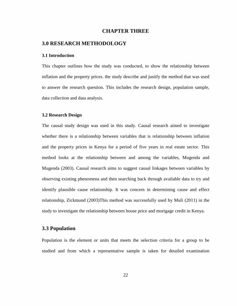
3.1 Introduction

This chapter outlines how the study was conducted, to show the relationship between

inflation and the property prices. the study describe and justify the method that was used

to answer the research question. This includes the research design, population sample,

data collection and data analysis.

3.2 Research Design

The causal study design was used in this study. Causal research aimed to investigate

whether there is a relationship between variables that is relationship between inflation

and the property prices in Kenya for a period of five years in real estate sector. This

method looks at the relationship between and among the variables, Mugenda and

Mugenda (2003). Causal research aims to suggest causal linkages between variables by

observing existing phenomena and then searching back through available data to try and

identify plausible cause relationship. It was concern in determining cause and effect

relationship, Zickmund (2003)This method was successfully used by Muli (2011) in the

study to investigate the relationship between house price and mortgage credit in Kenya.

3.3 Population

Population is the element or units that meets the selection criteria for a group to be

studied and from which a representative sample is taken for detailed examination

23

(Zickmund 2003) .The target population of interest in this study was 2,000 houses sold

in each area selected in Nairobi County.

3.4 Sample and sampling Technique

Sample is small groups whose characteristics are accurately reflect those of the larger

population from which it is drown ,King’oria ( 2004). In this research the sample was

2000 houses sold, for the period of five years from 2008 to 2012.This period is selected

due to the rapid growth of property prices, and also due to the instability of the Kenya

shilling which was attributed to the inflation, Hass Consult (2012). Judgmental sampling

method was used to come up with a representative sample; this method was successfully

used by Mwangi (2010). According to Zickmund (2003) judgmental sampling is the

selection of items on the basis of the judgment or opinion of one or more persons. It

enables one to select cases that will best answer the research question.

3.5 Data collection

Secondary data was used in this research. Property prices was collected from the ministry

Lands, Housing and Urban development, while inflation rates data was collected from the

Kenya National Bureau of statistic.

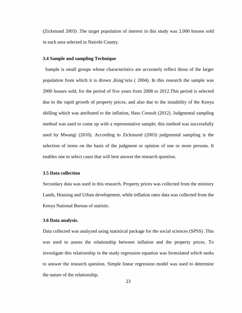
3.6 Data analysis.

Data collected was analyzed using statistical package for the social sciences (SPSS) .This

was used to assess the relationship between inflation and the property prices. To

investigate this relationship in the study regression equation was formulated which seeks

to answer the research question. Simple linear regression model was used to determine

the nature of the relationship.

24

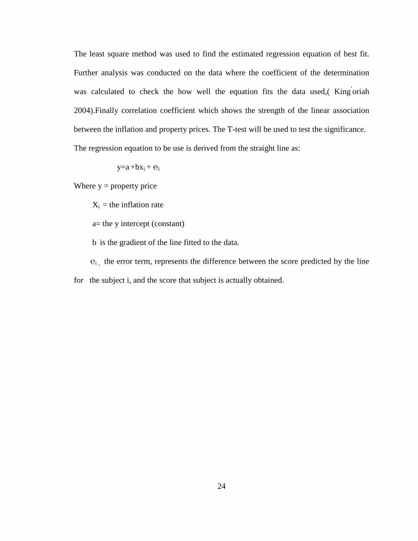
The least square method was used to find the estimated regression equation of best fit.

Further analysis was conducted on the data where the coefficient of the determination

was calculated to check the how well the equation fits the data used,( King’oriah

2004).Finally correlation coefficient which shows the strength of the linear association

between the inflation and property prices. The T-test will be used to test the significance.

The regression equation to be use is derived from the straight line as:

y=a +bxi + ℮i

Where y = property price

Xi = the inflation rate

a= the y intercept (constant)

b is the gradient of the line fitted to the data.

℮i , the error term, represents the difference between the score predicted by the line

for the subject i, and the score that subject is actually obtained.

25

CHAPTER FOUR

4.0 DATA ANALYSIS AND PRESENTATION OF THE FINDINGS.

4.1 Introduction

This chapter presents the research findings and conclusions of the causal study. The study

is centered on the relationship between inflation and property prices in Kenya. The study

was conducted on the data for Q1 to Q4 for the years 2008 to 2012. The price of the

property was analyzed in two set. This will give more accurate findings. Data from

Kileleswa, Lavington and Kilimani is analyzed and presented as section one while

section two represent Embakasi, Buruburu, Kasarani and South B & C.

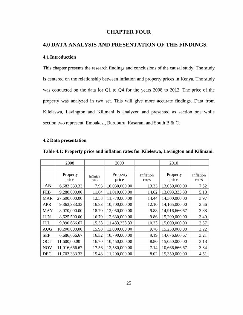
4.2 Data presentation

Table 4.1: Property price and inflation rates for Kileleswa, Lavington and Kilimani.

2008 2009 2010

Property

price Inflation

rates

Property price

Inflation rates

Property price

Inflation rates

JAN 6,683,333.33 7.93 10,030,000.00 13.33 13,050,000.00 7.52

FEB 9,280,000.00 11.04 11,010,000.00 14.62 13,693,333.33 5.18

MAR 27,600,000.00 12.53 11,770,000.00 14.44 14,300,000.00 3.97

APR 9,363,333.33 16.83 10,700,000.00 12.10 14,165,000.00 3.66

MAY 8,070,000.00 18.70 12,050,000.00 9.88 14,916,666.67 3.88

JUN 8,625,500.00 16.79 12,630,000.00 9.86 15,200,000.00 3.49

JUL 9,890,666.67 15.33 11,433,333.33 10.33 15,000,000.00 3.57

AUG 10,200,000.00 15.98 12,000,000.00 9.76 15,230,000.00 3.22

SEP 6,686,666.67 16.32 10,790,000.00 9.19 14,676,666.67 3.21

OCT 11,600,00.00 16.70 10,450,000.00 8.80 15,050,000.00 3.18

NOV 11,016,666.67 17.56 12,580,000.00 7.14 10,666,666.67 3.84

DEC 11,703,333.33 15.48 11,200,000.00 8.02 15,350,000.00 4.51

26

2011 2012

inflation Inflation

rates rates

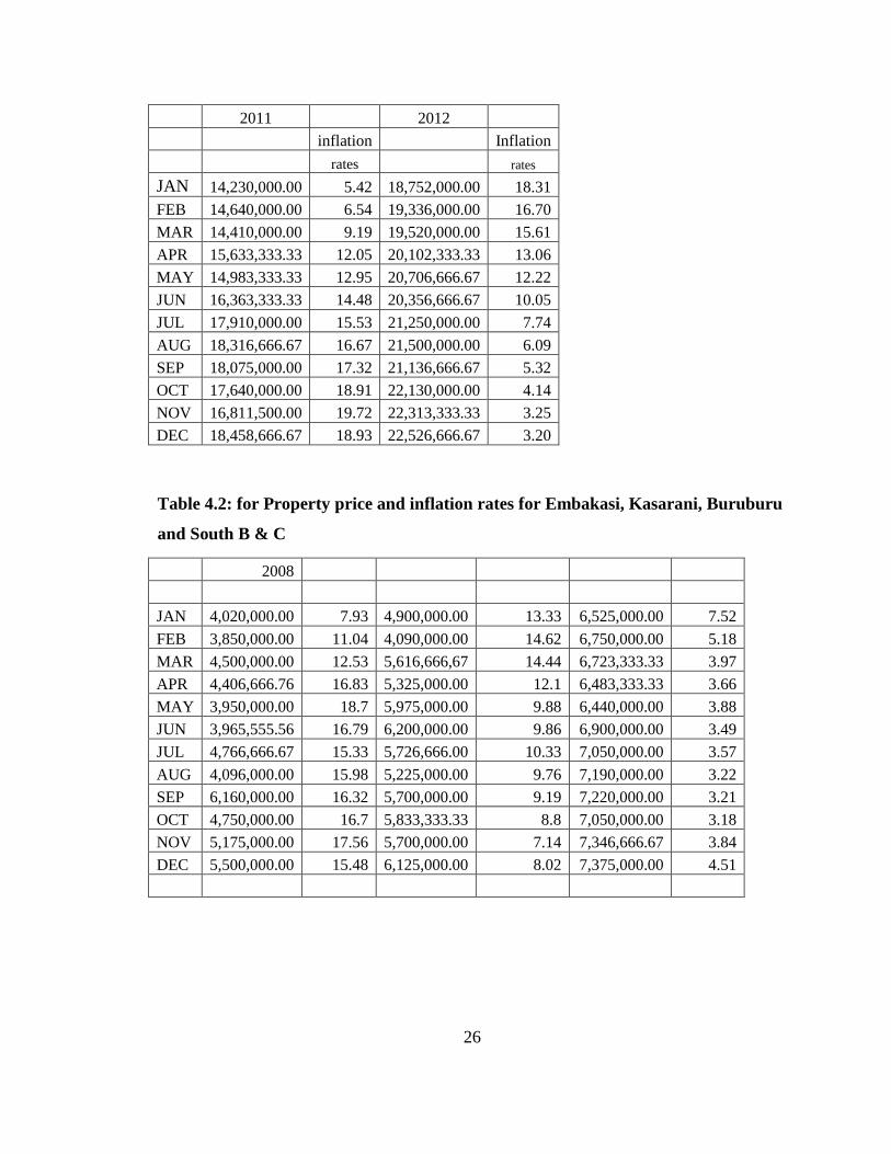
JAN 14,230,000.00 5.42 18,752,000.00 18.31

FEB 14,640,000.00 6.54 19,336,000.00 16.70

MAR 14,410,000.00 9.19 19,520,000.00 15.61

APR 15,633,333.33 12.05 20,102,333.33 13.06

MAY 14,983,333.33 12.95 20,706,666.67 12.22

JUN 16,363,333.33 14.48 20,356,666.67 10.05

JUL 17,910,000.00 15.53 21,250,000.00 7.74

AUG 18,316,666.67 16.67 21,500,000.00 6.09

SEP 18,075,000.00 17.32 21,136,666.67 5.32

OCT 17,640,000.00 18.91 22,130,000.00 4.14

NOV 16,811,500.00 19.72 22,313,333.33 3.25

DEC 18,458,666.67 18.93 22,526,666.67 3.20

Table 4.2: for Property price and inflation rates for Embakasi, Kasarani, Buruburu

and South B & C

2008

JAN 4,020,000.00 7.93 4,900,000.00 13.33 6,525,000.00 7.52

FEB 3,850,000.00 11.04 4,090,000.00 14.62 6,750,000.00 5.18

MAR 4,500,000.00 12.53 5,616,666,67 14.44 6,723,333.33 3.97

APR 4,406,666.76 16.83 5,325,000.00 12.1 6,483,333.33 3.66

MAY 3,950,000.00 18.7 5,975,000.00 9.88 6,440,000.00 3.88

JUN 3,965,555.56 16.79 6,200,000.00 9.86 6,900,000.00 3.49

JUL 4,766,666.67 15.33 5,726,666.00 10.33 7,050,000.00 3.57

AUG 4,096,000.00 15.98 5,225,000.00 9.76 7,190,000.00 3.22

SEP 6,160,000.00 16.32 5,700,000.00 9.19 7,220,000.00 3.21

OCT 4,750,000.00 16.7 5,833,333.33 8.8 7,050,000.00 3.18

NOV 5,175,000.00 17.56 5,700,000.00 7.14 7,346,666.67 3.84

DEC 5,500,000.00 15.48 6,125,000.00 8.02 7,375,000.00 4.51

27

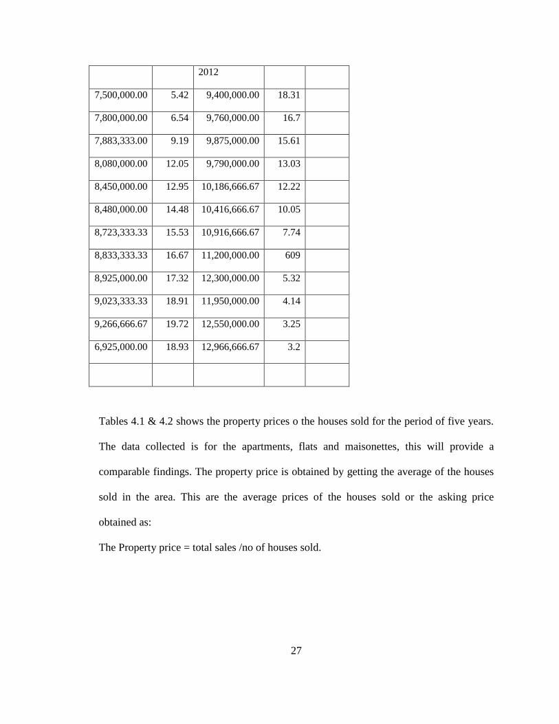
2012

7,500,000.00 5.42 9,400,000.00 18.31

7,800,000.00 6.54 9,760,000.00 16.7

7,883,333.00 9.19 9,875,000.00 15.61

8,080,000.00 12.05 9,790,000.00 13.03

8,450,000.00 12.95 10,186,666.67 12.22

8,480,000.00 14.48 10,416,666.67 10.05

8,723,333.33 15.53 10,916,666.67 7.74

8,833,333.33 16.67 11,200,000.00 609

8,925,000.00 17.32 12,300,000.00 5.32

9,023,333.33 18.91 11,950,000.00 4.14

9,266,666.67 19.72 12,550,000.00 3.25

6,925,000.00 18.93 12,966,666.67 3.2

Tables 4.1 & 4.2 shows the property prices o the houses sold for the period of five years.

The data collected is for the apartments, flats and maisonettes, this will provide a

comparable findings. The property price is obtained by getting the average of the houses

sold in the area. This are the average prices of the houses sold or the asking price

obtained as:

The Property price = total sales /no of houses sold.

28

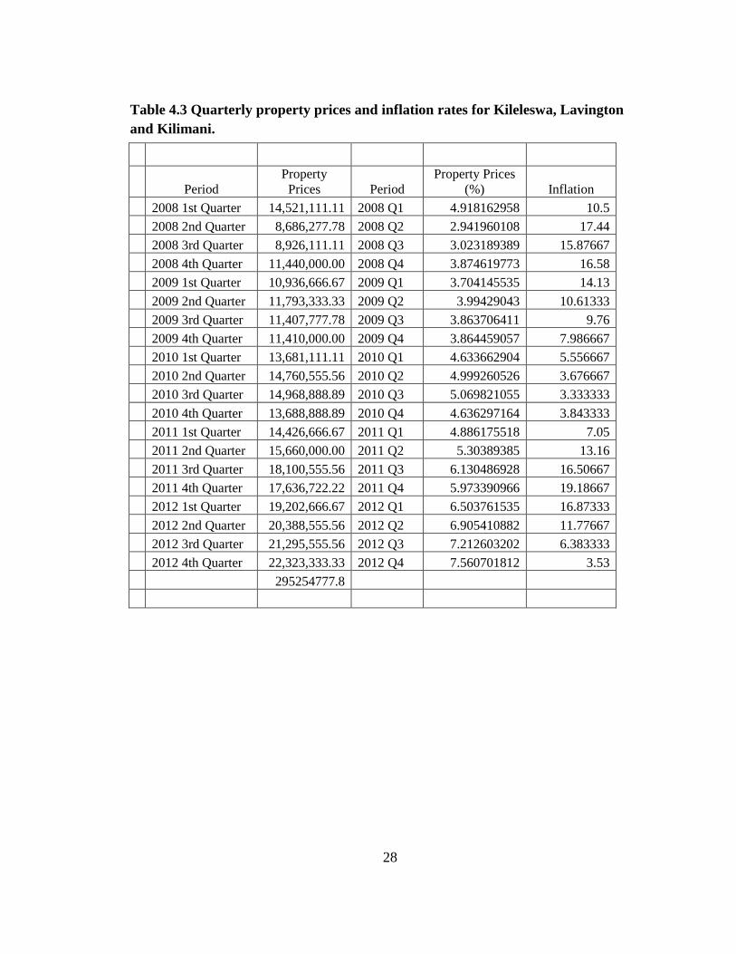
Table 4.3 Quarterly property prices and inflation rates for Kileleswa, Lavington and Kilimani.

Period Property Prices Period

Property Prices (%) Inflation

2008 1st Quarter 14,521,111.11 2008 Q1 4.918162958 10.5

2008 2nd Quarter 8,686,277.78 2008 Q2 2.941960108 17.44

2008 3rd Quarter 8,926,111.11 2008 Q3 3.023189389 15.87667

2008 4th Quarter 11,440,000.00 2008 Q4 3.874619773 16.58

2009 1st Quarter 10,936,666.67 2009 Q1 3.704145535 14.13

2009 2nd Quarter 11,793,333.33 2009 Q2 3.99429043 10.61333

2009 3rd Quarter 11,407,777.78 2009 Q3 3.863706411 9.76

2009 4th Quarter 11,410,000.00 2009 Q4 3.864459057 7.986667

2010 1st Quarter 13,681,111.11 2010 Q1 4.633662904 5.556667

2010 2nd Quarter 14,760,555.56 2010 Q2 4.999260526 3.676667

2010 3rd Quarter 14,968,888.89 2010 Q3 5.069821055 3.333333

2010 4th Quarter 13,688,888.89 2010 Q4 4.636297164 3.843333

2011 1st Quarter 14,426,666.67 2011 Q1 4.886175518 7.05

2011 2nd Quarter 15,660,000.00 2011 Q2 5.30389385 13.16

2011 3rd Quarter 18,100,555.56 2011 Q3 6.130486928 16.50667

2011 4th Quarter 17,636,722.22 2011 Q4 5.973390966 19.18667

2012 1st Quarter 19,202,666.67 2012 Q1 6.503761535 16.87333

2012 2nd Quarter 20,388,555.56 2012 Q2 6.905410882 11.77667

2012 3rd Quarter 21,295,555.56 2012 Q3 7.212603202 6.383333

2012 4th Quarter 22,323,333.33 2012 Q4 7.560701812 3.53

295254777.8

29

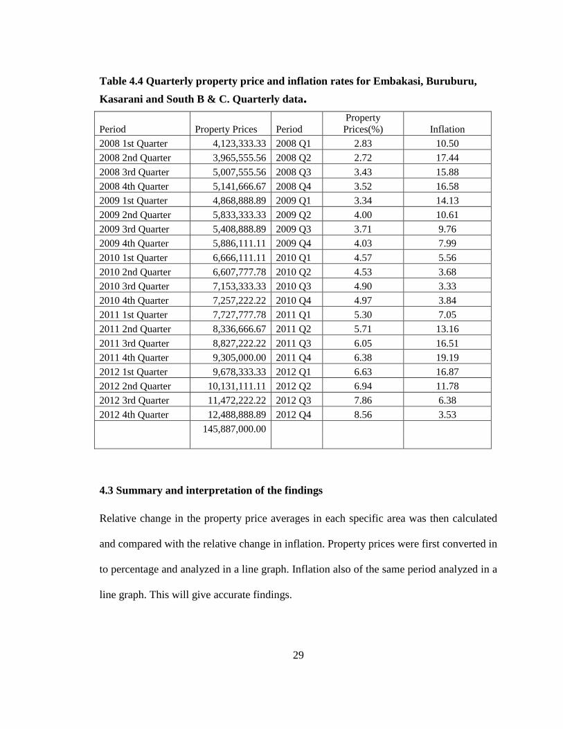
Table 4.4 Quarterly property price and inflation rates for Embakasi, Buruburu,

Kasarani and South B & C. Quarterly data.

Period Property Prices Period Property Prices(%) Inflation

2008 1st Quarter 4,123,333.33 2008 Q1 2.83 10.50

2008 2nd Quarter 3,965,555.56 2008 Q2 2.72 17.44

2008 3rd Quarter 5,007,555.56 2008 Q3 3.43 15.88

2008 4th Quarter 5,141,666.67 2008 Q4 3.52 16.58

2009 1st Quarter 4,868,888.89 2009 Q1 3.34 14.13

2009 2nd Quarter 5,833,333.33 2009 Q2 4.00 10.61

2009 3rd Quarter 5,408,888.89 2009 Q3 3.71 9.76

2009 4th Quarter 5,886,111.11 2009 Q4 4.03 7.99

2010 1st Quarter 6,666,111.11 2010 Q1 4.57 5.56

2010 2nd Quarter 6,607,777.78 2010 Q2 4.53 3.68

2010 3rd Quarter 7,153,333.33 2010 Q3 4.90 3.33

2010 4th Quarter 7,257,222.22 2010 Q4 4.97 3.84

2011 1st Quarter 7,727,777.78 2011 Q1 5.30 7.05

2011 2nd Quarter 8,336,666.67 2011 Q2 5.71 13.16

2011 3rd Quarter 8,827,222.22 2011 Q3 6.05 16.51

2011 4th Quarter 9,305,000.00 2011 Q4 6.38 19.19

2012 1st Quarter 9,678,333.33 2012 Q1 6.63 16.87

2012 2nd Quarter 10,131,111.11 2012 Q2 6.94 11.78

2012 3rd Quarter 11,472,222.22 2012 Q3 7.86 6.38

2012 4th Quarter 12,488,888.89 2012 Q4 8.56 3.53

145,887,000.00

4.3 Summary and interpretation of the findings

Relative change in the property price averages in each specific area was then calculated

and compared with the relative change in inflation. Property prices were first converted in

to percentage and analyzed in a line graph. Inflation also of the same period analyzed in a

line graph. This will give accurate findings.

Figure 4.1: property prices and inflation movement from 2008 to 2012.

The figure below represent the data analysis for Kileleswa, Lavington and Kilimani area.

Figure 4.1: Data Analysis for Kileleswa, Lavington and Kilimani

30

1: property prices and inflation movement from 2008 to 2012.

The figure below represent the data analysis for Kileleswa, Lavington and Kilimani area.

Analysis for Kileleswa, Lavington and Kilimani

The figure below represent the data analysis for Kileleswa, Lavington and Kilimani area.

Figure 4.2: property prices and inflation rates movements from 2008 to 2012For

Embakasi, Kasarani, Buruburu, Mombasa road, South B and C.

Figure 4.2 Property prices and inflation movement

From the graph above we can observe that the property prices have been on a continuous

increase over the years. Between Q1 to Q3 of 2008 there was a slight drop and stagnation

while the inflation rose gradually reaching its highest level. In Q4 2008 to Q1 of 2010,

the property prices were still increasing gradually where as inflation rates declines in the

same quarters reaching its dip in between the second and the third quarters of 2010.

The charts also indicate that there was a gradual increase in property prices in Q1

all through to the last quarter of 2012. (Q4). While inflation rates rose it peak of 19% in

the fourth quarter of 2011 before taking a sharp dip to 3.2% in the last quarter of 2012

31

Figure 4.2: property prices and inflation rates movements from 2008 to 2012For

Embakasi, Kasarani, Buruburu, Mombasa road, South B and C.

Figure 4.2 Property prices and inflation movement

above we can observe that the property prices have been on a continuous

increase over the years. Between Q1 to Q3 of 2008 there was a slight drop and stagnation

while the inflation rose gradually reaching its highest level. In Q4 2008 to Q1 of 2010,

roperty prices were still increasing gradually where as inflation rates declines in the

same quarters reaching its dip in between the second and the third quarters of 2010.

The charts also indicate that there was a gradual increase in property prices in Q1

all through to the last quarter of 2012. (Q4). While inflation rates rose it peak of 19% in

the fourth quarter of 2011 before taking a sharp dip to 3.2% in the last quarter of 2012

Figure 4.2: property prices and inflation rates movements from 2008 to 2012For

above we can observe that the property prices have been on a continuous

increase over the years. Between Q1 to Q3 of 2008 there was a slight drop and stagnation

while the inflation rose gradually reaching its highest level. In Q4 2008 to Q1 of 2010,

roperty prices were still increasing gradually where as inflation rates declines in the

same quarters reaching its dip in between the second and the third quarters of 2010.

The charts also indicate that there was a gradual increase in property prices in Q1 2011

all through to the last quarter of 2012. (Q4). While inflation rates rose it peak of 19% in

the fourth quarter of 2011 before taking a sharp dip to 3.2% in the last quarter of 2012

32

this display a negative correlation. These extreme variations which were observed could

have been due to the fiscal and monetary policies by the government through Central

Bank o Kenya in an effort to meet their macroeconomic goal of price stability.

This research objective is to find out if there is any relationship between property prices

and inflation from the findings it can be observed that there is no clear defined

relationship between the property prices and inflation rates.

From the analysis of variance (ANOVA) statistic the study shows that the processed data

has the significant level. This indicates that the data is ideal for making conclusion and it

also shows that the data sampled represent the population. We can observe that the

regression sum of squares is very huge implying that much of the variability is actually

accounted for in this regression model. The p-value=0.000<0.05 (significance level)

indicating that the model is appropriate and significant.

4.4 Summary of the study

The objectives of the study was to find out whether property prices change are related to

change in inflation. Its observed that property prices has been on a continuous increase

over the years but gradually while inflation rate rose sharply to its peak (double digit

)highest of 19.72% in the last quarter of 2012. It has been fluctuating to extreme

variations. The findings of this study shows that there is no clear relationship between

the property price and the inflation rate in contrary Muli (2011) in his study of the

relationship between property prices and the mortgage lending in Kenya, his findings

33

indicate that the relationship between evolution of mortgage lending and the house price

is well established.

Omboi (2011) in the study of impacts of inflation on the cost of mortgage financing, his

findings shows that higher inflation would have a negative impact on housing prices.

High inflation rates affect the repayment of the mortgage principle and increase the real

value repayment this raise the demand for property. Piazzessi and Schneider (2012) in

their study of inflation and property of real asset found out that these changes in inflation

expectations make housing more attractive, because of the capital gains, taxes and

mortgage deductibility.

34

CHAPTER FIVE

5.0 SUMMARY, CONCLUSION AND RECOMENTATIONS

5.1 Summary

Real estate is one of the most vibrant and profitable in the world today. The growth has

been driven by urbanization, a strong economy and significant credit expansion. This

project sought to investigate the relationship between property prices and inflation rates.

Property prices fluctuations has been associated with the housing boom and bust and the

financial instability which has been experienced by many countries in the world. The

study also explains the types of inflation and its effects in the real estate market. The

study review theories and the empirical evidence of various researchers, these enhance an

insight understanding of the research problem.

This study used secondary data on property prices which was collected from the ministry

of Land, Housing and Urban Development, Hassconsult and Value zones limited.

Inflation rate data was collected from the Kenya National Bureau of statistics. All this

was analyzed by regression analysis to determine whether there is a relationship between

property prices and inflation rates. Judgmental sampling was used to get the sample and

the target population was the apartments and mansionetts which are more common in the

selected area.

35

The study concluded that a property price has been on continuous increase over the years

but at a gradual phase. While the inflation rates increased sharply and dropping sharply.

This shows that there is no clear defined relationship between inflation rates and property

prices.

5.2 Conclusion

The aim of the study was to investigate the relationship between property price and

inflation rates. It is observed that property price have been continuously increasing

gradually while inflation rates has been fluctuating, it stabilized in the last quarter of

2012 due to the government fiscal and monitory policies through central bank in an effort

to meet microeconomic goal of price stability.

The movement of property prices was not consistent with inflation rates. Inflation rates

change movement were sometimes very high while the property price low and gradually

increasing this draws a conclusion of this causal study that there were no clear defined

relationship between property price and inflation rates. There are several factors

influencing property prices this is why the results were not clear.

5.3 Policy recommendations.

Property is an attractive investment asset that investors should include in there portfolio.

According to this study property prices were not affected by the inflation hence the

Government should set policies to encourage people to invest in real asset like property

so has to edge inflation when it is high.

36

Property price has been increasing over the years hence the Government should set up

policies towards ensuring that every Kenyan has real asset which he/ she can afford. This

can be achieved by setting up policies that can control property pricing.

The purchase and ownership of property depend largely on the availability and cost of

mortgage. Mortgage rates should be controlled by the Government through CBK. Central

Bank of Kenya should consider exploring more prescriptive rules which would set some

minimum standards for mortgage loans in terms of both loan to value and payment to

income. Lastly the Government should set standards which ensure full disclosure of

information pertaining rates, terms and conditions, fees and charges on properties in

Kenya. This would stabilize the real estate market.

5.4 Limitations of the study.

Lack of local studies on the relationship between property price and inflation rates. The

study relied on the international studies. The Kenyan government should encourage more

studies in the real estate market, since its one of the fastest growing market. This was a

causal study and the findings may not be representative of the country. The focus was

Nairobi county and due to lack of data from previous years period to 2008, the study was

only carried out for five years this is a restrictive short period. More time would have

been more reliable in making generalization.

37

Real estate market is influenced by factors such as import duty, land price, proximity to

the major highway population and the exchange rates. This makes every investor comes

up with his or her own price. Also the price may have been bargained downwards from

the asking price i.e. the government are discounted and this will not reflect the market.

Inconsistency in data collection was another limiting factor in this study. The average

data obtained from the available months was therefore used to make reference for the

whole quarter. Data collection was not consistent for some moths and therefore not

reflecting the market trends.

5.5 Suggestions for further studies.

From the research findings of these studies, the real estate market is vast and very few

researches has been done especially in Kenya. This study targeted the apartments and the

mansionet only further research should be done on town houses and all types to compare

the trends in the industry.

A research on other factors that influence property prices should also be conducted. This

should include the level of development in the area, proximity to the tarmac road, which

are the main highways in Kenya. The same such research should also be carried out in the

major towns in Kenya such as Kisumu, Mombasa, Kericho ,Nakuru and Eldoret. This

will have a larger sample and the findings will reflect the real estate market clearly.

38

REFFERENCES

Brown, G., and Matysiak, G. (1999), “Real Estate Investment. A capital Market

Approach Financial Times”, London.

Burnside, Greig, Martin, E., and S. Rebelo (2011), “Understanding Booms and Busts

in Housing Markets’’, NBER Working paper 16734 (Cambridge

Masschusetts; National Bureau of Economic Research).

Chin, T.L., (2002). “A critical review of literature on Hedonic Price Model and its

Application to the Housing Market in Penang”.

Crane, A., J., Hartzell. (2008), “Is there Disposition Effect in corporate investment

Decision? Evidence from Real Estate Investment Trust”, Working Paper. The

University of Texas at Austin.

Daniel Ojijo (2011), “Homes Kenya”, Magazine available in web- www.homeske.

Deydorce Syryah (2010), MBA Project on “Strategic response by national housing

corporation on the effects of global economic meltdown on housing in

Kenya”, University of Nairobi unpublished.

Fama Eugene F (1970), “Efficient Market a review of theory and Empirical Work”,

Journal of significance 25; 385-450

Fama, E. F., Fisher L., Jensen M., and Roll R., (1969), “The Adjustment of stock

Prices to New Information”, International Economic Review 10(1):1 to 21.

Fred, Brett Johnson (1997), “The wealth power of property”, published ISBN

Genosover, David & Christopher Mayer. (2001), “Loss aversion and seller behavior.

Evidence from the housing Market”, Quarterly journal of economic 116

(4);1233-1260

39

Gordon, Myron. J. (1962), “The Investment, Financing and Valuation of the

Corporation” Homewood. III: Irwin.

Greer, G,. E. Farrell; M, D. (1983), “Investment Analysis of Real Estate Decisions.

Dearbon Financial Pub Inc”. Contemporary Real Estate Theory and Practice,

Dryden Press,

Hass consult, (2012), “The Hass Property Index: Quarter one Report 2012”,

Available in www.hassconsult.co.ke.

Henneberry, J and Rowley, S. (2002), “Property Market Prosses and Development

outcomes in cities and Regions”, Londo, Royal Institute of Chartered

Surveyors.

Hertzell, D.J. Hekman and M. Miles (1978), “Real estate returns and Inflation journal

of the American Real Estate and Urbarn Economics Association”.

Jeniffer N. Muli (2011), MBA project on “The relationship between house prices and

mortgage credit in Kenya”, University of Nairobi unpublished

Kahneman. D,. A.,Tversky. (1979). Prospect Theory; “An analysis of decision under

risk”, Econometrical 47:263-297.

Karl, Case and, R. Shiller, (1989). “The Behavior of Rome Buyers in boom and post

boom Markets,”NBER Working Paper 2748, National Bureau of Economic

Research, Inc

Karuri Waweru (2012)., “The ABC of Real Estate Investment in Kenya”, Economic

Journal , www.tradeinvestoafrica.com

Lebaron. D,. (1999)., “Investors Psychology. Available on line”:

htt:/www.deanlebaron.com

40

Malpezzi, S and Wachter, S (2005), “The role of speculation in Real Estate Cycle,

Zell/Lurie Center Working Paper 401”, Wharton School of Management,

University of Pennylvania.

Milton Friedman and A. J. Schwartz (1963), “A mornitory History of the united

state”, The Princeton University Press.

Moris, A, (2007), “Land Prices in Westlands Worry Investor’s Business daily”,

Available on web, www.adafrica.com

Mugenda, O.M., Mugenda, A. G (2003), “Research Methods, Quantitative and

Qualitative Approaches”, Acts Press, Nairobi.

Muth, J.F. (1961), “Rational Expectation and the National Office Market”, AREVA

Journal, 15 (4): 281-299

Plazzi, A., Torous. W., Volkanov, R., 92006), “Expected return and Expected Growth

in Rents of Commercial Real Estate”. Working Paper. University of Califonia-

Los Ageles.

Richmond, D,. (1994), “Introduction to Valuation, (3rd ed). Macmillan Press”, LTD

Sheifer, A,. (2000). “Inefficient Market: An In Introduction of Behavioral Finance.

Oxford Press”, Oxford.

Shiller, R. J. (2005), “Irrational Exuberance (2nd ed). Princeon University Press,

Princeton and Oxford”.

Syagga, P. M. (1994). “Real Estate Valuation Handbook: with special Reference to

Kenya”, Nairobi University Press.

T. A. Johnson,. K. Davies, E. F,. Shapiro (2000), “Modern Methods of Valuation,( 9th

ed)” . London.

T. Pearson, Stephen F., Terry G. (1995), “Market Analysis for Valuation Appraisal”.

Appraisal Institute of Chicago.

41

Tversky, A,. and D. Kahneman. (1991). “Loss Aversion in Riskless Choice: A

Reference-Dependent Model”, Quarterly Journal of Economics 106: 1039-

106.

Whipple, R. T. M. (1995), “A Property Valuation Analysis. The Law Book

Company”.

Zickmud, William G. (2003). “Business research methods, 7th edition, Southwestern.

42

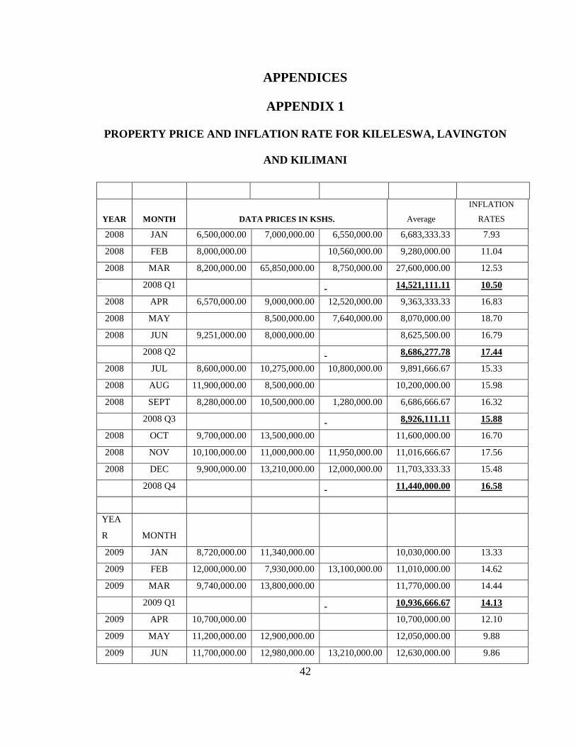
APPENDICES

APPENDIX 1

PROPERTY PRICE AND INFLATION RATE FOR KILELESWA, LAVINGTON

AND KILIMANI

YEAR MONTH DATA PRICES IN KSHS. Average

INFLATION

RATES

2008 JAN 6,500,000.00 7,000,000.00 6,550,000.00 6,683,333.33 7.93

2008 FEB 8,000,000.00 10,560,000.00 9,280,000.00 11.04

2008 MAR 8,200,000.00 65,850,000.00 8,750,000.00 27,600,000.00 12.53

2008 Q1 14,521,111.11 10.50

2008 APR 6,570,000.00 9,000,000.00 12,520,000.00 9,363,333.33 16.83

2008 MAY 8,500,000.00 7,640,000.00 8,070,000.00 18.70

2008 JUN 9,251,000.00 8,000,000.00 8,625,500.00 16.79

2008 Q2 8,686,277.78 17.44

2008 JUL 8,600,000.00 10,275,000.00 10,800,000.00 9,891,666.67 15.33

2008 AUG 11,900,000.00 8,500,000.00 10,200,000.00 15.98

2008 SEPT 8,280,000.00 10,500,000.00 1,280,000.00 6,686,666.67 16.32

2008 Q3 8,926,111.11 15.88

2008 OCT 9,700,000.00 13,500,000.00 11,600,000.00 16.70

2008 NOV 10,100,000.00 11,000,000.00 11,950,000.00 11,016,666.67 17.56

2008 DEC 9,900,000.00 13,210,000.00 12,000,000.00 11,703,333.33 15.48

2008 Q4 11,440,000.00 16.58

YEA

R MONTH

2009 JAN 8,720,000.00 11,340,000.00 10,030,000.00 13.33

2009 FEB 12,000,000.00 7,930,000.00 13,100,000.00 11,010,000.00 14.62

2009 MAR 9,740,000.00 13,800,000.00 11,770,000.00 14.44

2009 Q1 10,936,666.67 14.13

2009 APR 10,700,000.00 10,700,000.00 12.10

2009 MAY 11,200,000.00 12,900,000.00 12,050,000.00 9.88

2009 JUN 11,700,000.00 12,980,000.00 13,210,000.00 12,630,000.00 9.86

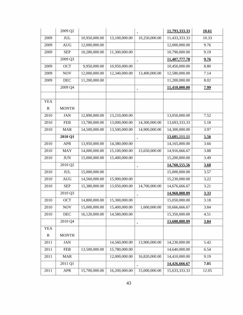
43

2009 Q2 11,793,333.33 10.61

2009 JUL 10,950,000.00 13,100,000.00 10,250,000.00 11,433,333.33 10.33

2009 AUG 12,000,000.00 12,000,000.00 9.76

2009 SEP 10,280,000.00 11,300,000.00 10,790,000.00 9.19

2009 Q3 11,407,777.78 9.76

2009 OCT 9,950,000.00 10,950,000.00 10,450,000.00 8.80

2009 NOV 12,000,000.00 12,340,000.00 13,400,000.00 12,580,000.00 7.14

2009 DEC 11,200,000.00 11,200,000.00 8.02

2009 Q4 11,410,000.00 7.99

YEA

R MONTH

2010 JAN 12,890,000.00 13,210,000.00 13,050,000.00 7.52

2010 FEB 13,780,000.00 13,000,000.00 14,300,000.00 13,693,333.33 5.18

2010 MAR 14,500,000.00 13,500,000.00 14,900,000.00 14,300,000.00 3.97

2010 Q1 13,681,111.11 5.56

2010 APR 13,950,000.00 14,380,000.00 14,165,000.00 3.66

2010 MAY 14,000,000.00 15,100,000.00 15,650,000.00 14,916,666.67 3.88

2010 JUN 15,000,000.00 15,400,000.00 15,200,000.00 3.49

2010 Q2 14,760,555.56 3.68

2010 JUL 15,000,000.00 15,000,000.00 3.57

2010 AUG 14,560,000.00 15,900,000.00 15,230,000.00 3.22

2010 SEP 15,380,000.00 13,950,000.00 14,700,000.00 14,676,666.67 3.21

2010 Q3 14,968,888.89 3.33

2010 OCT 14,800,000.00 15,300,000.00 15,050,000.00 3.18

2010 NOV 15,000,000.00 15,400,000.00 1,600,000.00 10,666,666.67 3.84

2010 DEC 16,120,000.00 14,580,000.00 15,350,000.00 4.51

2010 Q4 13,688,888.89 3.84

YEA

R MONTH

2011 JAN 14,560,000.00 13,900,000.00 14,230,000.00 5.42

2011 FEB 13,500,000.00 15,780,000.00 14,640,000.00 6.54

2011 MAR 12,000,000.00 16,820,000.00 14,410,000.00 9.19

2011 Q1 14,426,666.67 7.05

2011 APR 15,700,000.00 16,200,000.00 15,000,000.00 15,633,333.33 12.05

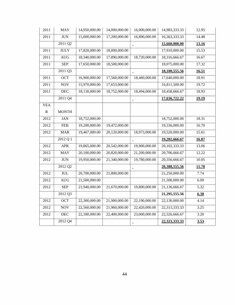
44

2011 MAY 14,950,000.00 14,000,000.00 16,000,000.00 14,983,333.33 12.95

2011 JUN 15,000,000.00 17,200,000.00 16,890,000.00 16,363,333.33 14.48

2011 Q2 15,660,000.00 13.16

2011 JULY 17,820,000.00 18,000,000.00 17,910,000.00 15.53

2011 AUG 18,340,000.00 17,890,000.00 18,720,000.00 18,316,666.67 16.67

2011 SEP 17,650,000.00 18,500,000.00 18,075,000.00 17.32

2011 Q3 18,100,555.56 16.51

2011 OCT 16,900,000.00 17,560,000.00 18,460,000.00 17,640,000.00 18.91

2011 NOV 15,970,000.00 17,653,000.00 16,811,500.00 19.72

2011 DEC 18,130,000.00 18,752,000.00 18,494,000.00 18,458,666.67 18.93

2011 Q4 17,636,722.22 19.19

YEA

R MONTH

2012 JAN 18,752,000.00 18,752,000.00 18.31

2012 FEB 19,200,000.00 19,472,000.00 19,336,000.00 16.70

2012 MAR 19,467,000.00 20,120,000.00 18,973,000.00 19,520,000.00 15.61

2012 Q 1 19,202,666.67 16.87

2012 APR 19,865,000.00 20,542,000.00 19,900,000.00 20,102,333.33 13.06

2012 MAY 20,100,000.00 20,820,000.00 21,200,000.00 20,706,666.67 12.22

2012 JUN 19,950,000.00 21,340,000.00 19,780,000.00 20,356,666.67 10.05

2012 Q2 20,388,555.56 11.78

2012 JUL 20,700,000.00 21,800,000.00 21,250,000.00 7.74

2012 AUG 21,500,000.00 21,500,000.00 6.09

2012 SEP 21,940,000.00 21,670,000.00 19,800,000.00 21,136,666.67 5.32

2012 Q3 21,295,555.56 6.38

2012 OCT 22,300,000.00 21,900,000.00 22,190,000.00 22,130,000.00 4.14

2012 NOV 22,560,000.00 21,960,000.00 22,420,000.00 22,313,333.33 3.25

2012 DEC 22,180,000.00 22,400,000.00 23,000,000.00 22,526,666.67 3.20

2012 Q4 22,323,333.33 3.53

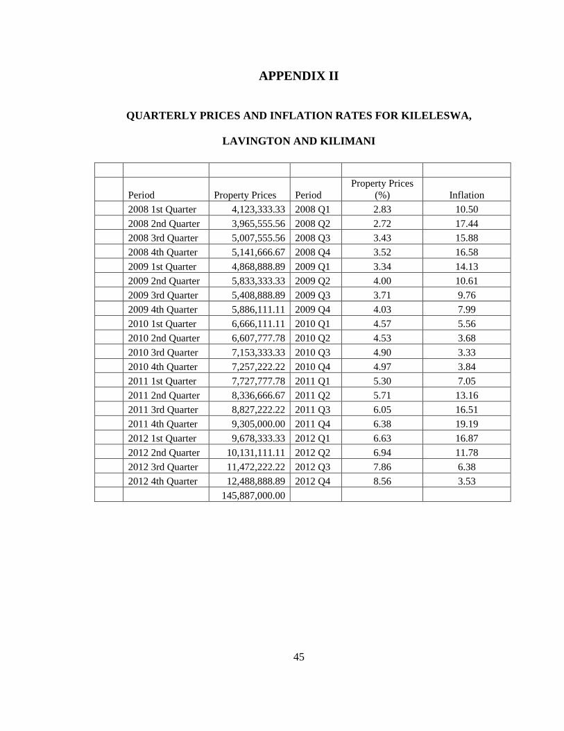
45

APPENDIX II

QUARTERLY PRICES AND INFLATION RATES FOR KILELESWA,

LAVINGTON AND KILIMANI

Period Property Prices Period Property Prices

(%) Inflation

2008 1st Quarter 4,123,333.33 2008 Q1 2.83 10.50

2008 2nd Quarter 3,965,555.56 2008 Q2 2.72 17.44

2008 3rd Quarter 5,007,555.56 2008 Q3 3.43 15.88

2008 4th Quarter 5,141,666.67 2008 Q4 3.52 16.58

2009 1st Quarter 4,868,888.89 2009 Q1 3.34 14.13

2009 2nd Quarter 5,833,333.33 2009 Q2 4.00 10.61

2009 3rd Quarter 5,408,888.89 2009 Q3 3.71 9.76

2009 4th Quarter 5,886,111.11 2009 Q4 4.03 7.99

2010 1st Quarter 6,666,111.11 2010 Q1 4.57 5.56

2010 2nd Quarter 6,607,777.78 2010 Q2 4.53 3.68

2010 3rd Quarter 7,153,333.33 2010 Q3 4.90 3.33

2010 4th Quarter 7,257,222.22 2010 Q4 4.97 3.84

2011 1st Quarter 7,727,777.78 2011 Q1 5.30 7.05

2011 2nd Quarter 8,336,666.67 2011 Q2 5.71 13.16

2011 3rd Quarter 8,827,222.22 2011 Q3 6.05 16.51

2011 4th Quarter 9,305,000.00 2011 Q4 6.38 19.19

2012 1st Quarter 9,678,333.33 2012 Q1 6.63 16.87

2012 2nd Quarter 10,131,111.11 2012 Q2 6.94 11.78

2012 3rd Quarter 11,472,222.22 2012 Q3 7.86 6.38

2012 4th Quarter 12,488,888.89 2012 Q4 8.56 3.53

145,887,000.00

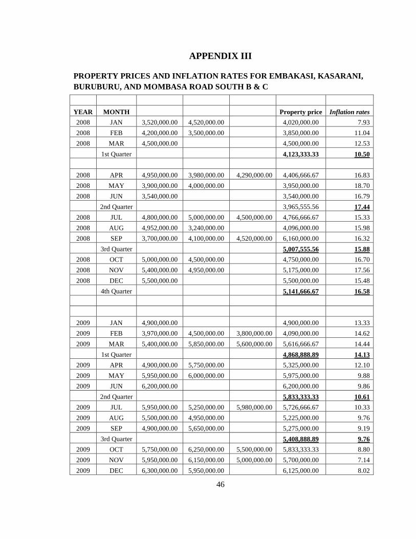
46

APPENDIX III

PROPERTY PRICES AND INFLATION RATES FOR EMBAKASI, KASARANI, BURUBURU, AND MOMBASA ROAD SOUTH B & C

YEAR MONTH Property price Inflation rates

2008 JAN 3,520,000.00 4,520,000.00 4,020,000.00 7.93

2008 FEB 4,200,000.00 3,500,000.00 3,850,000.00 11.04

2008 MAR 4,500,000.00 4,500,000.00 12.53

1st Quarter 4,123,333.33 10.50

2008 APR 4,950,000.00 3,980,000.00 4,290,000.00 4,406,666.67 16.83

2008 MAY 3,900,000.00 4,000,000.00 3,950,000.00 18.70

2008 JUN 3,540,000.00 3,540,000.00 16.79

2nd Quarter 3,965,555.56 17.44

2008 JUL 4,800,000.00 5,000,000.00 4,500,000.00 4,766,666.67 15.33

2008 AUG 4,952,000.00 3,240,000.00 4,096,000.00 15.98

2008 SEP 3,700,000.00 4,100,000.00 4,520,000.00 6,160,000.00 16.32

3rd Quarter 5,007,555.56 15.88

2008 OCT 5,000,000.00 4,500,000.00 4,750,000.00 16.70

2008 NOV 5,400,000.00 4,950,000.00 5,175,000.00 17.56

2008 DEC 5,500,000.00 5,500,000.00 15.48

4th Quarter 5,141,666.67 16.58

2009 JAN 4,900,000.00 4,900,000.00 13.33

2009 FEB 3,970,000.00 4,500,000.00 3,800,000.00 4,090,000.00 14.62

2009 MAR 5,400,000.00 5,850,000.00 5,600,000.00 5,616,666.67 14.44

1st Quarter 4,868,888.89 14.13

2009 APR 4,900,000.00 5,750,000.00 5,325,000.00 12.10

2009 MAY 5,950,000.00 6,000,000.00 5,975,000.00 9.88

2009 JUN 6,200,000.00 6,200,000.00 9.86

2nd Quarter 5,833,333.33 10.61

2009 JUL 5,950,000.00 5,250,000.00 5,980,000.00 5,726,666.67 10.33

2009 AUG 5,500,000.00 4,950,000.00 5,225,000.00 9.76

2009 SEP 4,900,000.00 5,650,000.00 5,275,000.00 9.19

3rd Quarter 5,408,888.89 9.76

2009 OCT 5,750,000.00 6,250,000.00 5,500,000.00 5,833,333.33 8.80

2009 NOV 5,950,000.00 6,150,000.00 5,000,000.00 5,700,000.00 7.14

2009 DEC 6,300,000.00 5,950,000.00 6,125,000.00 8.02

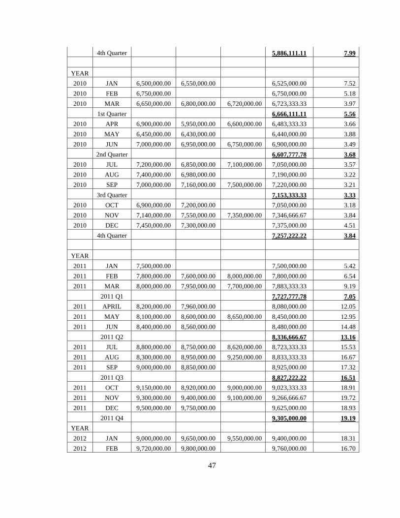
47

4th Quarter 5,886,111.11 7.99

YEAR

2010 JAN 6,500,000.00 6,550,000.00 6,525,000.00 7.52

2010 FEB 6,750,000.00 6,750,000.00 5.18

2010 MAR 6,650,000.00 6,800,000.00 6,720,000.00 6,723,333.33 3.97

1st Quarter 6,666,111.11 5.56

2010 APR 6,900,000.00 5,950,000.00 6,600,000.00 6,483,333.33 3.66

2010 MAY 6,450,000.00 6,430,000.00 6,440,000.00 3.88

2010 JUN 7,000,000.00 6,950,000.00 6,750,000.00 6,900,000.00 3.49

2nd Quarter 6,607,777.78 3.68

2010 JUL 7,200,000.00 6,850,000.00 7,100,000.00 7,050,000.00 3.57

2010 AUG 7,400,000.00 6,980,000.00 7,190,000.00 3.22

2010 SEP 7,000,000.00 7,160,000.00 7,500,000.00 7,220,000.00 3.21

3rd Quarter 7,153,333.33 3.33

2010 OCT 6,900,000.00 7,200,000.00 7,050,000.00 3.18

2010 NOV 7,140,000.00 7,550,000.00 7,350,000.00 7,346,666.67 3.84

2010 DEC 7,450,000.00 7,300,000.00 7,375,000.00 4.51

4th Quarter 7,257,222.22 3.84

YEAR

2011 JAN 7,500,000.00 7,500,000.00 5.42

2011 FEB 7,800,000.00 7,600,000.00 8,000,000.00 7,800,000.00 6.54

2011 MAR 8,000,000.00 7,950,000.00 7,700,000.00 7,883,333.33 9.19

2011 Q1 7,727,777.78 7.05

2011 APRIL 8,200,000.00 7,960,000.00 8,080,000.00 12.05

2011 MAY 8,100,000.00 8,600,000.00 8,650,000.00 8,450,000.00 12.95

2011 JUN 8,400,000.00 8,560,000.00 8,480,000.00 14.48

2011 Q2 8,336,666.67 13.16

2011 JUL 8,800,000.00 8,750,000.00 8,620,000.00 8,723,333.33 15.53

2011 AUG 8,300,000.00 8,950,000.00 9,250,000.00 8,833,333.33 16.67

2011 SEP 9,000,000.00 8,850,000.00 8,925,000.00 17.32

2011 Q3 8,827,222.22 16.51

2011 OCT 9,150,000.00 8,920,000.00 9,000,000.00 9,023,333.33 18.91

2011 NOV 9,300,000.00 9,400,000.00 9,100,000.00 9,266,666.67 19.72

2011 DEC 9,500,000.00 9,750,000.00 9,625,000.00 18.93

2011 Q4 9,305,000.00 19.19

YEAR

2012 JAN 9,000,000.00 9,650,000.00 9,550,000.00 9,400,000.00 18.31

2012 FEB 9,720,000.00 9,800,000.00 9,760,000.00 16.70

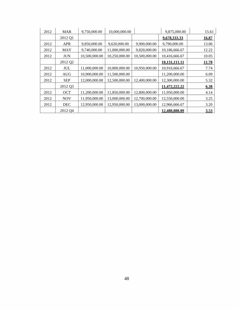
48

2012 MAR 9,750,000.00 10,000,000.00 9,875,000.00 15.61

2012 Q1 9,678,333.33 16.87

2012 APR 9,850,000.00 9,620,000.00 9,900,000.00 9,790,000.00 13.06

2012 MAY 9,740,000.00 11,000,000.00 9,820,000.00 10,186,666.67 12.22

2012 JUN 10,500,000.00 10,250,000.00 10,500,000.00 10,416,666.67 10.05

2012 Q2 10,131,111.11 11.78

2012 JUL 11,000,000.00 10,800,000.00 10,950,000.00 10,916,666.67 7.74

2012 AUG 10,900,000.00 11,500,000.00 11,200,000.00 6.09

2012 SEP 12,000,000.00 12,500,000.00 12,400,000.00 12,300,000.00 5.32

2012 Q3 11,472,222.22 6.38

2012 OCT 11,200,000.00 11,850,000.00 12,800,000.00 11,950,000.00 4.14

2012 NOV 11,950,000.00 13,000,000.00 12,700,000.00 12,550,000.00 3.25

2012 DEC 12,950,000.00 12,950,000.00 13,000,000.00 12,966,666.67 3.20

2012 Q4 12,488,888.89 3.53

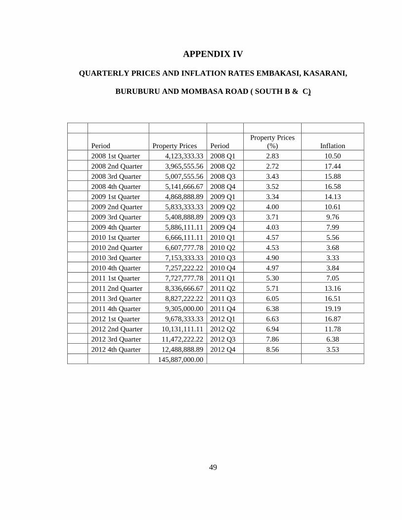
49

APPENDIX IV

QUARTERLY PRICES AND INFLATION RATES EMBAKASI, KASARANI,

BURUBURU AND MOMBASA ROAD ( SOUTH B & C)

Period Property Prices Period Property Prices

(%) Inflation

2008 1st Quarter 4,123,333.33 2008 Q1 2.83 10.50

2008 2nd Quarter 3,965,555.56 2008 Q2 2.72 17.44

2008 3rd Quarter 5,007,555.56 2008 Q3 3.43 15.88

2008 4th Quarter 5,141,666.67 2008 Q4 3.52 16.58

2009 1st Quarter 4,868,888.89 2009 Q1 3.34 14.13

2009 2nd Quarter 5,833,333.33 2009 Q2 4.00 10.61

2009 3rd Quarter 5,408,888.89 2009 Q3 3.71 9.76

2009 4th Quarter 5,886,111.11 2009 Q4 4.03 7.99

2010 1st Quarter 6,666,111.11 2010 Q1 4.57 5.56

2010 2nd Quarter 6,607,777.78 2010 Q2 4.53 3.68

2010 3rd Quarter 7,153,333.33 2010 Q3 4.90 3.33

2010 4th Quarter 7,257,222.22 2010 Q4 4.97 3.84

2011 1st Quarter 7,727,777.78 2011 Q1 5.30 7.05

2011 2nd Quarter 8,336,666.67 2011 Q2 5.71 13.16

2011 3rd Quarter 8,827,222.22 2011 Q3 6.05 16.51

2011 4th Quarter 9,305,000.00 2011 Q4 6.38 19.19

2012 1st Quarter 9,678,333.33 2012 Q1 6.63 16.87

2012 2nd Quarter 10,131,111.11 2012 Q2 6.94 11.78

2012 3rd Quarter 11,472,222.22 2012 Q3 7.86 6.38

2012 4th Quarter 12,488,888.89 2012 Q4 8.56 3.53

145,887,000.00

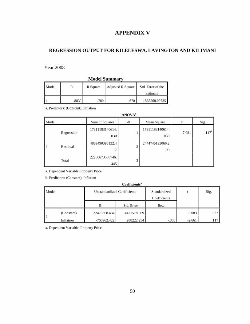
50

APPENDIX V

REGRESSION OUTPUT FOR KILELESWA, LAVINGTON AND KILIMANI

Year 2008

Model Summary

Model R R Square Adjusted R Square Std. Error of the

Estimate

1 .883a .780 .670 1563568.09735

a. Predictors: (Constant), Inflation

ANOVAa

Model Sum of Squares df Mean Square F Sig.

1

Regression 17311183140614.

030 1

17311183140614.

030 7.081 .117b

Residual 4889490390132.4

17 2

2444745195066.2

09

Total 22200673530746.

445 3

a. Dependent Variable: Property Price

b. Predictors: (Constant), Inflation

Coefficientsa

Model Unstandardized Coefficients Standardized

Coefficients

t Sig.

B Std. Error Beta

1 (Constant) 22473868.434 4421578.669 5.083 .037

Inflation -766962.422 288222.254 -.883 -2.661 .117

a. Dependent Variable: Property Price

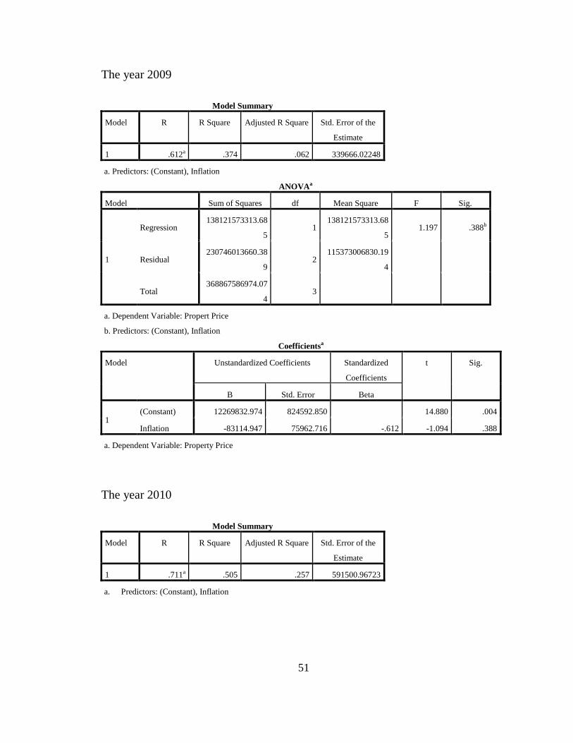
51

The year 2009

Model Summary

Model R R Square Adjusted R Square Std. Error of the

Estimate

1 .612a .374 .062 339666.02248

a. Predictors: (Constant), Inflation

ANOVAa

Model Sum of Squares df Mean Square F Sig.

1

Regression 138121573313.68

5 1

138121573313.68

5 1.197 .388b

Residual 230746013660.38

9 2

115373006830.19

4

Total 368867586974.07

4 3

a. Dependent Variable: Propert Price

b. Predictors: (Constant), Inflation

Coefficientsa

Model Unstandardized Coefficients Standardized

Coefficients

t Sig.

B Std. Error Beta

1 (Constant) 12269832.974 824592.850 14.880 .004

Inflation -83114.947 75962.716 -.612 -1.094 .388

a. Dependent Variable: Property Price

The year 2010

Model Summary

Model R R Square Adjusted R Square Std. Error of the

Estimate

1 .711a .505 .257 591500.96723

a. Predictors: (Constant), Inflation

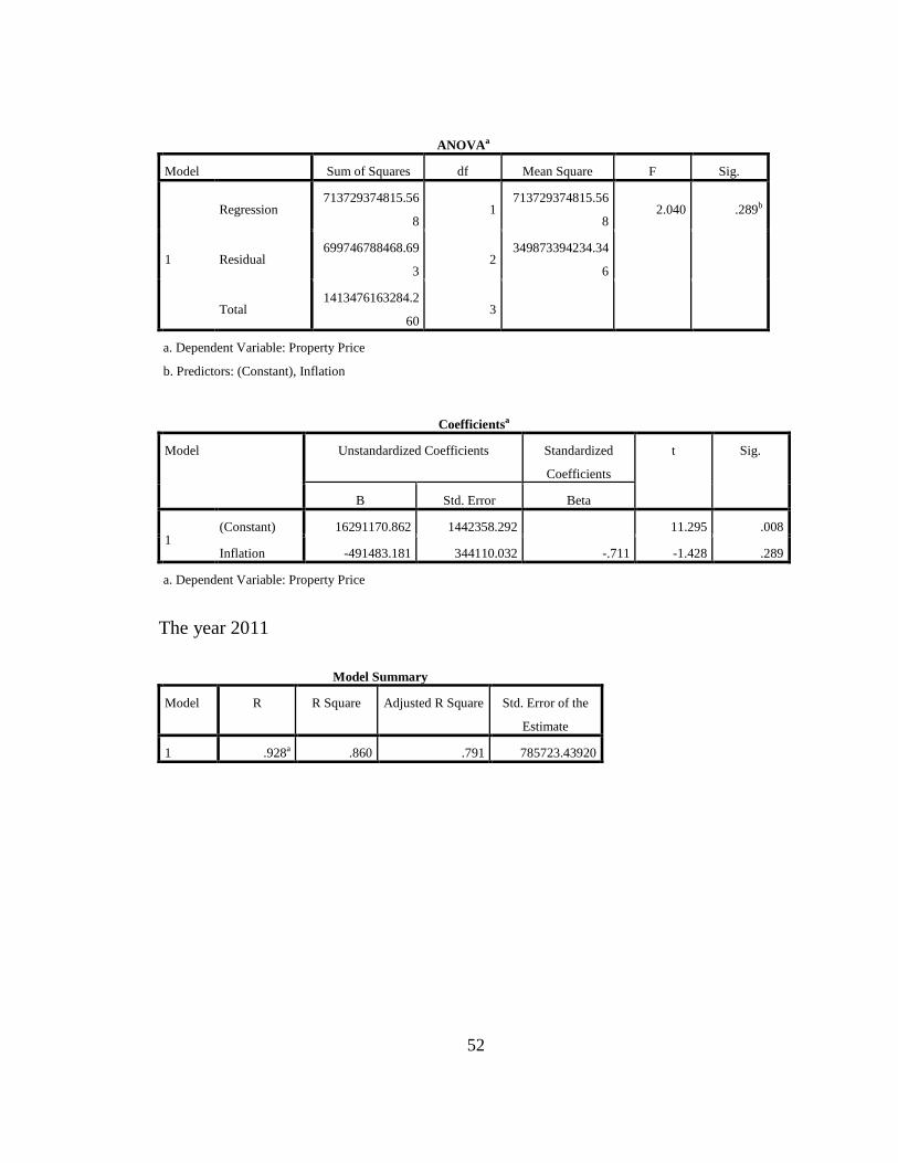
52

ANOVAa

Model Sum of Squares df Mean Square F Sig.

1

Regression 713729374815.56

8 1

713729374815.56

8 2.040 .289b

Residual 699746788468.69

3 2

349873394234.34

6

Total 1413476163284.2

60 3

a. Dependent Variable: Property Price

b. Predictors: (Constant), Inflation

Coefficientsa

Model Unstandardized Coefficients Standardized

Coefficients

t Sig.

B Std. Error Beta

1 (Constant) 16291170.862 1442358.292 11.295 .008

Inflation -491483.181 344110.032 -.711 -1.428 .289

a. Dependent Variable: Property Price

The year 2011

Model Summary

Model R R Square Adjusted R Square Std. Error of the

Estimate

1 .928a .860 .791 785723.43920

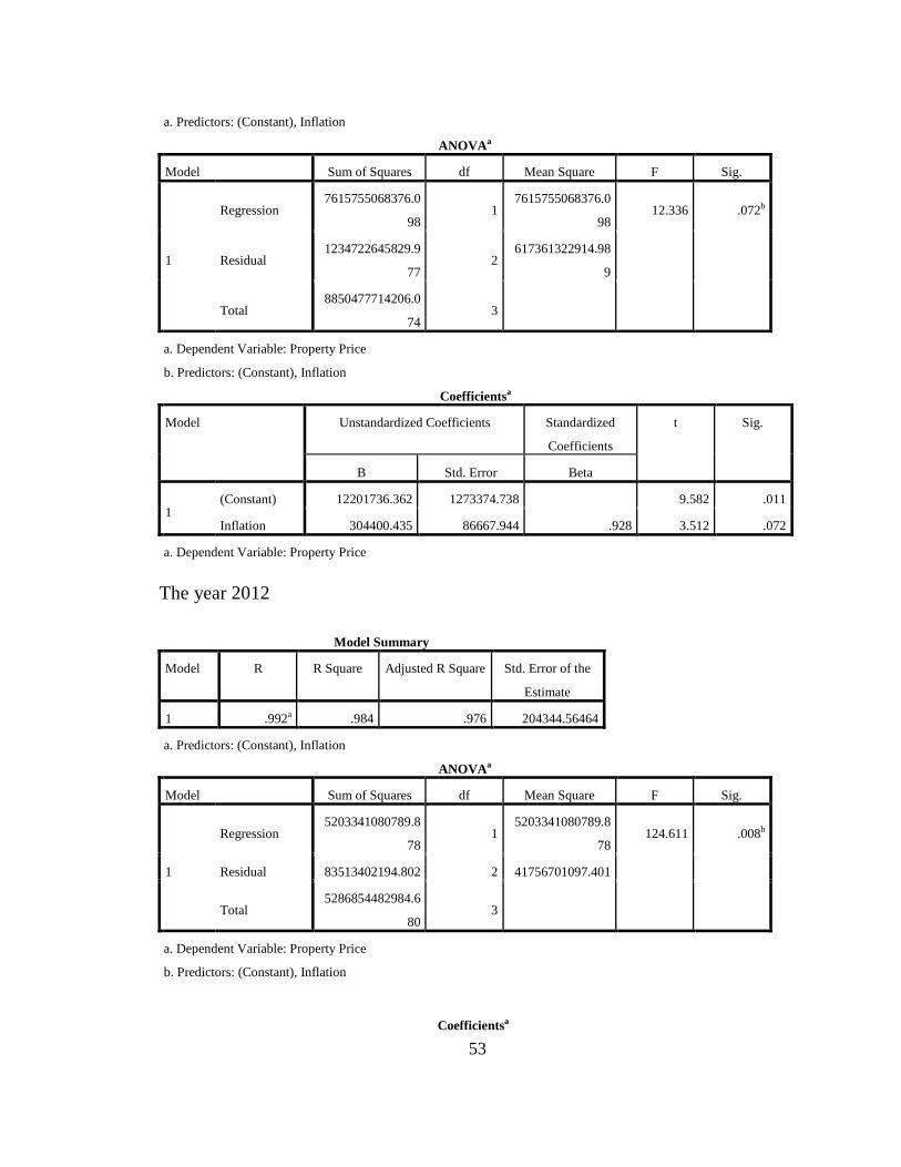
53

a. Predictors: (Constant), Inflation

ANOVAa

Model Sum of Squares df Mean Square F Sig.

1

Regression 7615755068376.0

98 1

7615755068376.0

98 12.336 .072b

Residual 1234722645829.9

77 2

617361322914.98

9

Total 8850477714206.0

74 3

a. Dependent Variable: Property Price

b. Predictors: (Constant), Inflation

Coefficientsa

Model Unstandardized Coefficients Standardized

Coefficients

t Sig.

B Std. Error Beta

1 (Constant) 12201736.362 1273374.738 9.582 .011

Inflation 304400.435 86667.944 .928 3.512 .072

a. Dependent Variable: Property Price

The year 2012

Model Summary

Model R R Square Adjusted R Square Std. Error of the

Estimate

1 .992a .984 .976 204344.56464

a. Predictors: (Constant), Inflation

ANOVAa

Model Sum of Squares df Mean Square F Sig.

1

Regression 5203341080789.8

78 1

5203341080789.8

78 124.611 .008b

Residual 83513402194.802 2 41756701097.401

Total 5286854482984.6

80 3

a. Dependent Variable: Property Price

b. Predictors: (Constant), Inflation

Coefficientsa

54

Model Unstandardized Coefficients Standardized

Coefficients

t Sig.

B Std. Error Beta

1 (Constant) 22950479.259 217862.304 105.344 .000

Inflation -222797.284 19958.681 -.992 -11.163 .008

a. Dependent Variable: Property Price

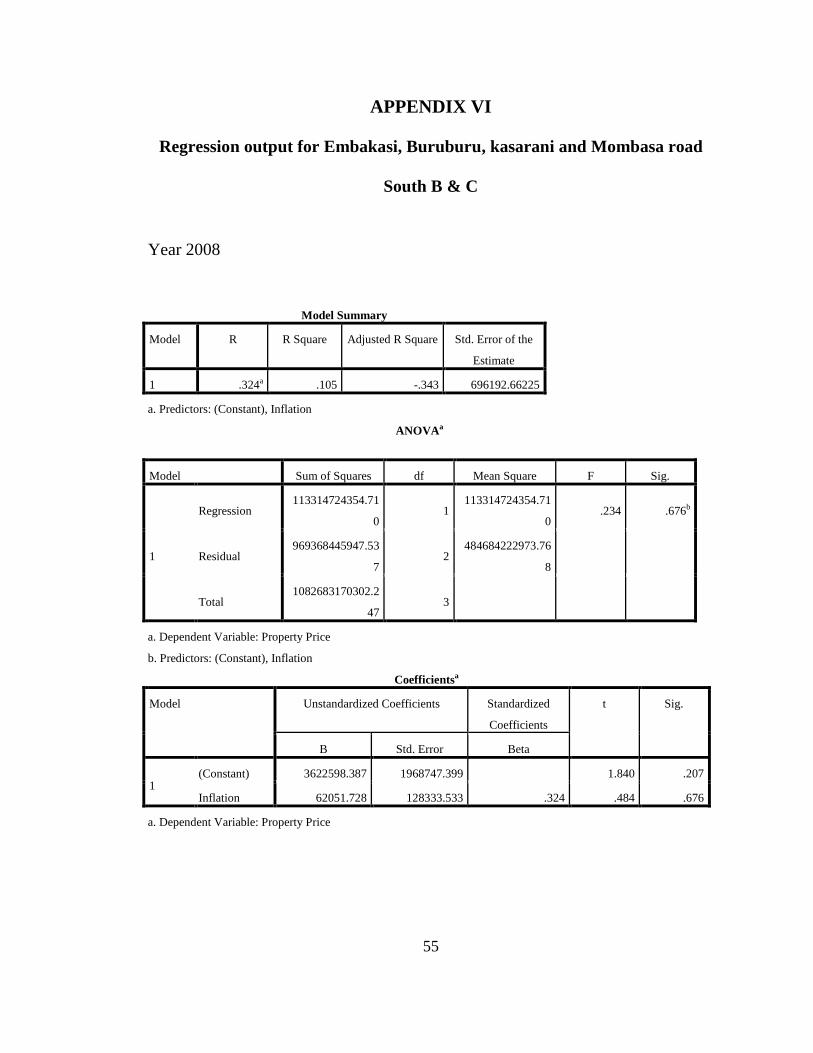
55

APPENDIX VI

Regression output for Embakasi, Buruburu, kasarani and Mombasa road

South B & C

Year 2008

Model Summary

Model R R Square Adjusted R Square Std. Error of the

Estimate

1 .324a .105 -.343 696192.66225

a. Predictors: (Constant), Inflation

ANOVAa

Model Sum of Squares df Mean Square F Sig.

1

Regression 113314724354.71

0 1

113314724354.71

0 .234 .676b

Residual 969368445947.53

7 2

484684222973.76

8

Total 1082683170302.2

47 3

a. Dependent Variable: Property Price

b. Predictors: (Constant), Inflation

Coefficientsa

Model Unstandardized Coefficients Standardized

Coefficients

t Sig.

B Std. Error Beta

1 (Constant) 3622598.387 1968747.399 1.840 .207

Inflation 62051.728 128333.533 .324 .484 .676

a. Dependent Variable: Property Price

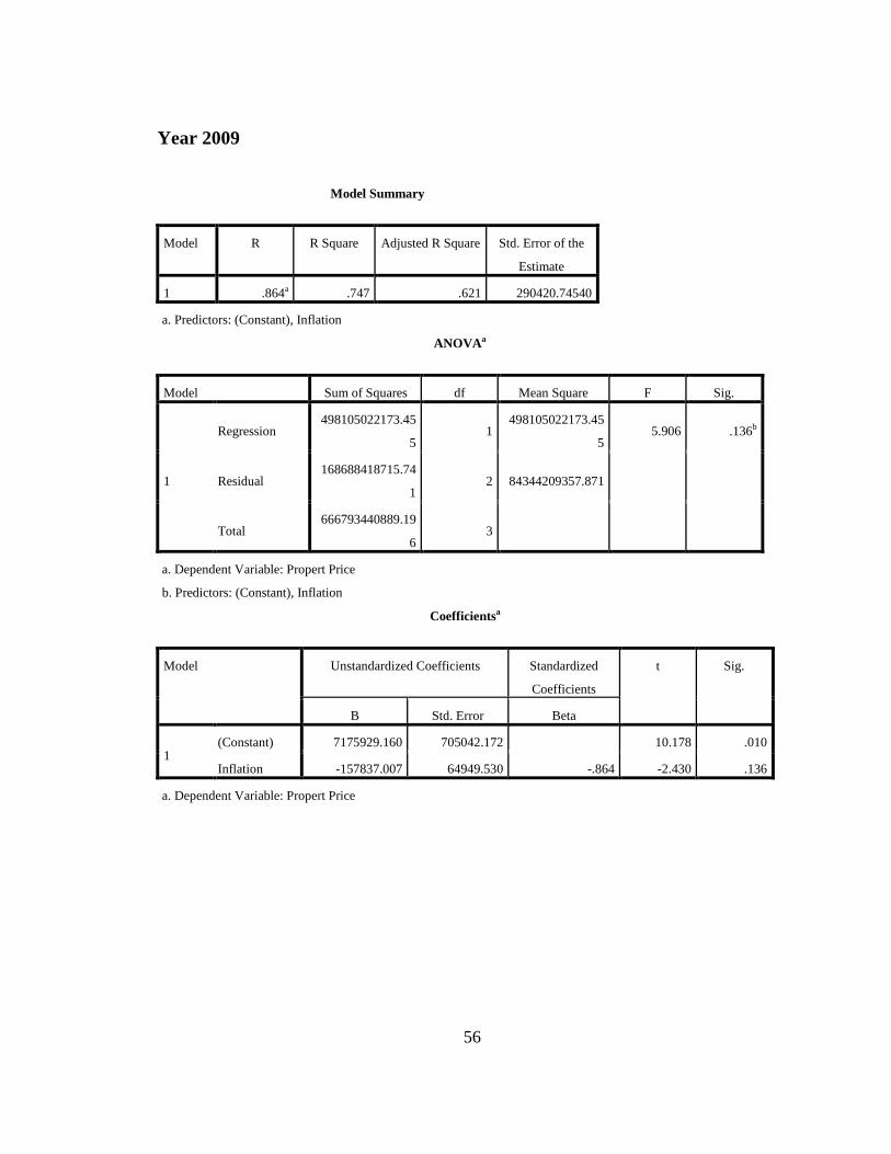
56

Year 2009

Model Summary

Model R R Square Adjusted R Square Std. Error of the

Estimate

1 .864a .747 .621 290420.74540

a. Predictors: (Constant), Inflation

ANOVAa

Model Sum of Squares df Mean Square F Sig.

1

Regression 498105022173.45

5 1

498105022173.45

5 5.906 .136b

Residual 168688418715.74

1 2 84344209357.871

Total 666793440889.19

6 3

a. Dependent Variable: Propert Price

b. Predictors: (Constant), Inflation

Coefficientsa

Model Unstandardized Coefficients Standardized

Coefficients

t Sig.

B Std. Error Beta

1 (Constant) 7175929.160 705042.172 10.178 .010

Inflation -157837.007 64949.530 -.864 -2.430 .136

a. Dependent Variable: Propert Price

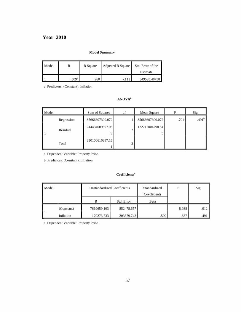
57

Year 2010

Model Summary

Model R R Square Adjusted R Square Std. Error of the

Estimate

1 .509a .260 -.111 349595.48738

a. Predictors: (Constant), Inflation

ANOVAa

Model Sum of Squares df Mean Square F Sig.

1

Regression 85666607300.072 1 85666607300.072 .701 .491b

Residual 244434009597.08

9 2

122217004798.54

5

Total 330100616897.16

1 3

a. Dependent Variable: Property Price

b. Predictors: (Constant), Inflation

Coefficientsa

Model Unstandardized Coefficients Standardized

Coefficients

t Sig.

B Std. Error Beta

1 (Constant) 7619659.103 852478.657 8.938 .012

Inflation -170273.733 203379.742 -.509 -.837 .491

a. Dependent Variable: Property Price

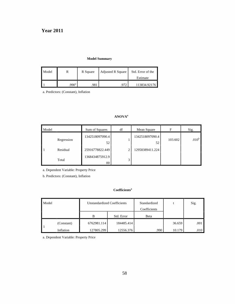
58

Year 2011

Model Summary

Model R R Square Adjusted R Square Std. Error of the

Estimate

1 .990a .981 .972 113834.92176

a. Predictors: (Constant), Inflation

ANOVAa

Model Sum of Squares df Mean Square F Sig.

1

Regression 1342518097090.4

52 1

1342518097090.4

52 103.602 .010b

Residual 25916778822.449 2 12958389411.224

Total 1368434875912.9

00 3

a. Dependent Variable: Property Price

b. Predictors: (Constant), Inflation

Coefficientsa

Model Unstandardized Coefficients Standardized

Coefficients

t Sig.

B Std. Error Beta

1 (Constant) 6762981.114 184485.414 36.659 .001

Inflation 127805.299 12556.376 .990 10.179 .010

a. Dependent Variable: Property Price

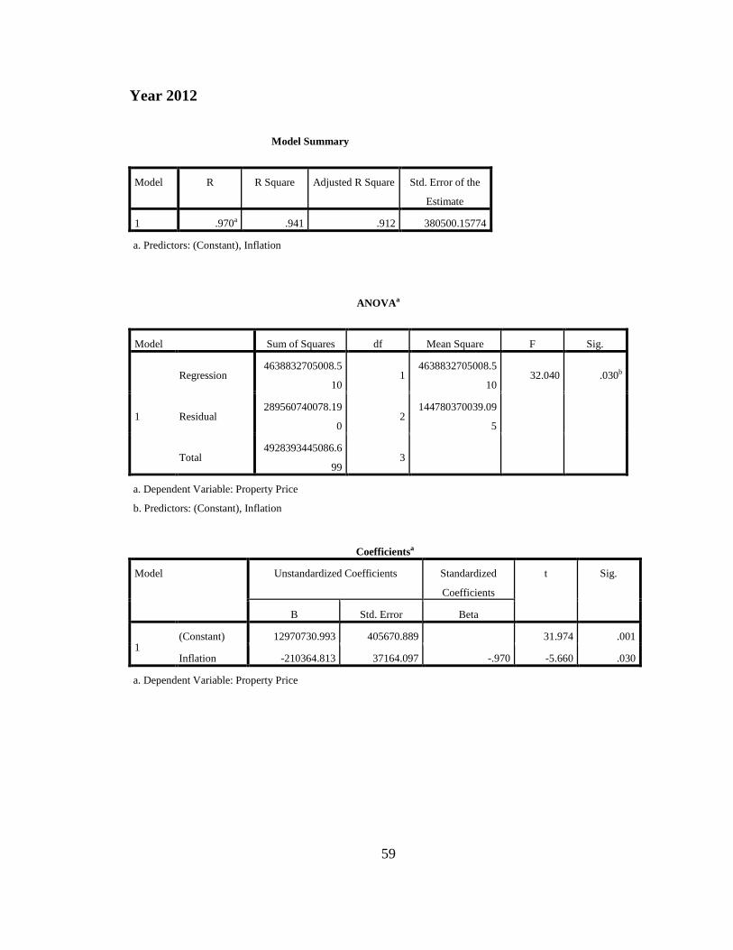
59

Year 2012

Model Summary

Model R R Square Adjusted R Square Std. Error of the

Estimate

1 .970a .941 .912 380500.15774

a. Predictors: (Constant), Inflation

ANOVAa

Model Sum of Squares df Mean Square F Sig.

1

Regression 4638832705008.5

10 1

4638832705008.5

10 32.040 .030b

Residual 289560740078.19

0 2

144780370039.09

5

Total 4928393445086.6

99 3

a. Dependent Variable: Property Price

b. Predictors: (Constant), Inflation

Coefficientsa

Model Unstandardized Coefficients Standardized

Coefficients

t Sig.

B Std. Error Beta

1 (Constant) 12970730.993 405670.889 31.974 .001

Inflation -210364.813 37164.097 -.970 -5.660 .030

a. Dependent Variable: Property Price