Embed Size (px)
Citation preview

IMPLEMENTATION OF FEEDFORWARD AND PID CONTROL STRATEGIES ON
CONTROL LOOP FIELDBUS FOUNDATION PROTOCOL
By
HAFFIZZULL RAHMAN BIN MD YUSUB
FINAL PROJECT REPORT
Submitted to the Electrical & Electronics Engineering Programme in Partial Fulfillment of the Requirements
for the Degree
Bachelor of Engineering (Hons) (Electrical & Electronics Engineering)
Universiti Teknologi Petronas
Bandar Seri Iskandar
31750 Tronoh
Perak Darul Ridzuan
© Copyright 2006
by
HaffiZZUII Rahman bin Md Yusub, December 2006

CERTIFICATION OF APPROVAL
IMPLEMENTATION OF FEEDFORW ARD AND PID CONTROL STRATEGIES ON CONTROL LOOP FIELDBUS FOUNDATION PROTOCOL
Approved by,
by
Haffizzull Rahman bin Md Yusub
A project dissertation submitted to the
Electrical & Electronics Engineering Programme
Universiti Teknologi PETRONAS
in partial fulfilment of the requirement for the
Bachelor of Engineering (Hons)
(Electrical & Electronics Engineering)
(Dr. Nordin bin Saad)
Project Supervisor.
UNIVERSITI TEKNOLOGI PETRONAS
TRONOH, PERAK
December 2006

CERTIFICATION OF ORIGINALITY
This is certify that I am responsible for the work submitted in this project, that the
original work is my own except as specified in the references and acknowledgements,
and that the original work contained herein have not been undertaken or done by
unspecified sources or person.
HafflZZUil Rahman bin Md Yusub
3355

ABSTRACT
This report is intended to discuss the project undertaken to design, analyse and
fabricate a simple control loop using a fieldbus foundation protocol. The first control
systems used mechanical and pneumatic controllers and were designed merely to
achieve stability rather than economic performance. Later in the 1970s, distributed
control system (DCS) emerged to replace the conventional technology. In DCS, a
central processor controls all parameters however, it has limitation in term of
reliability, robustness and cost. This lead to the introduction of network
communication for industrial process known as the fieldbus system replacing the
DCS architecture by enabling distribution of control function to equipment in the
field such as sensors, controllers and actuators. In this project configuration and
implementation procedure for the development of fieldbus process loop is presented
involving three process variables that are the temperature, pressure and level together
with PID and feedforward control strategies. The methodology towards
accomplishing the project includes the theoretical and technical research, the
installation and commissioning, the configuration network of fieldbus protocol
together with HART protocol, the troubleshooting, operation and maintenance, and
the analysis of the fieldbus advantages and benefits. The findings demonstrates the
benefits of the fieldbus system in term of cost saving, data quality and quantity,
simpler and better controllability.

ACKNOWLEDGEMENTS
First of all I would like to express my gratitude to Allah S.W.T for letting me
to complete my Final Year Project. Next, I would like to express my deepest
gratitude to my project supervisor Dr. Nordin bin Saad for guiding me to undergo my
project.
I would like also to express the greatest appreciation to all parties who have
contributed towards the success of this project. I also wish to thank those individuals
that play an important role in this project. Their guidance, advice, ideas and support
had become the most valuable experience and I really appreciate it. They are:
• Mr. Peter A Heffer, Principle Engineer, Instrument & Control, PETRONAS
Carigali KLCC (PCSB)
• Mr. Murugesan Karupparma, Senior Instrument Engineer of PETRONAS
Carigali KLCC (PCSB)
• Encik Djohan bin Arifin, my Plant Supervisor during Internship Program
• Mrs. Siti Hawa Haji Mohd Tahir, Lab Technologist. Electrical & Electronics
Department, Universiti Teknologi PETRONAS
• Mr. Azhar Zainal Abidin, Lab Technologist Plant Process, Universiti Teknologi
PETRONAS
• All supporting staffs in the Surface Engineering Department and Electrical and
Electronics Department
My appreciation also goes to Universiti Teknologi Petronas (UTP) especially
Electrical and Electronics Engineering Department, for endowing me with essential
skills to excel in theoretical and technical work. Last but not least, to all PCSB
trainees, friends and family who have been supporting me throughout this Final Year
Project.
ii

TABLE OF CONTENTS
ABSTRACT .................................................................................... .i
ACKNOWLEDGEMENTS .............................................................. ... .ii
TABLE OF CONTENTS .................................................................... iii
LIST OF FIGURES ......................................................................... .. vi
LIST OF TABLES .......................................................................... . .ix
LIST OF ABBREVIATION ................................................................. x
CHAPfER 1 INTRODUCTION ............................................................ 1
1.1 Background of Study ................................................... .. 1
1.2 Problem Statement ....................................................... 2
1.3 Objective and Scope of Study ......................................... .3
CHAPfER 2 LITERATURE REVIEWffHEORY ........................................ 5
2.1 Introduction ofFieldbus ................................................................ 5
2.2 Advantages ofFieldbus .................................................. 6
2.3 Fieldbus Topologies .................................................... 10
2.3.1 Point-to PointTopo1ogy ..................................... lO
2.3.2 Bus with Spurs Topology .................................. .11
2.3.3 Daisy-Chain Topology ...................................... l2
2.3.4 Tree Topology ................................................ l2
CHAPfER 3 METHODOLOGY/PROJECT WORK .................................. 13
3.1 Project Work ............................................................ 13
3.1.1 Research and Information Gathering ..................... l4
3.1.2 Control Loop Design ....................................... 14
3.1.3 Installation, Commissioning and Configuration ......... l4
3.1.4 Troubleshooting, Maintenance and Operation .......... .l4
3.2 Tools Required ......................................................... 15
3.2.1 Cable ........................................................... .l5
3.2.2 Terminal Blocks .............................................. .16
3.2.3 Terminators (BT302) ........................................ .17
iii

3.2.4 Host Devices ................................................... 18
3.2.5 Switch .......................................................... 18
3.2.6 Close and Open Tank ........................................ 19
3.2.7 System Configurator (SYSCON) ........................... 20
3.2.8 !CONICS GraphWorx32 .................................... 21
3.2.9 Fieldbus Universal Bridge (DFI-302) ..................... 21
3.2.1 0 HART Communicator ........................................ 23
3 .2.11 CA 100 Calibrator. ............................................ 24
3.2.12 YS136 Yokogawa Controller ............................... 24
3.2.13 URlOOO Recorder ............................................. 25
3.2.14 Measurement and Control Devices ......................... 26
CHAPTER 4 PROCESS PLANT AND ITS CONTROL STRATEGIES ............ 29
4.1 Petrobras Platform P-36 Explosion, Brazil.. ......................... 29
4.1.1 The Explosion and Fire ......................................... .30
4.2 Fire Water Pump Control System ...................................... 31
4.3 HART .................................................................... .32
4.4 Control Strategy Design and Configuration ........................ 35
4.4.1 PID Controller ................................................. .36
4.4.2 Feedforward Control.. ....................................... .38
4.4.3 Ratio Control.. ................................................ .39
4.4.4 Cascade Control. ............................................... 40
CHAPTER 5 INSTALLATION AND COMMISSIONING .......................... .42
5.1 Decommissioning Existing Plant.. .............•....•............... .42
5.2 Painting Process ....................................................... .43
5.3 Hardware and Piping Installation .................................... .43
5.4 Network Installation ................................................... .44
5.4.1 Establishing Loop Connections for HART Network
Wiring ........................................................... .44
5.4.2 Foundation Fieldbus Network Wiring ....................... 48
iv

CHAPTER6 SYSTEM CONFIGURATION AND INTERFACING ..... .Sl
6.1 Foundation Fieldbus Configuration ................................... 51
6.1.1 Initializing Initial Communication ........................... 52
6.1.2 Uploading Fieldbus Network and Devices ................. 53
6.2 Device Commissioning ................................................ 55
6.2.1 Changing Device Attribute ................................... 55
6.2.2 Creating the Function Block .................................. 56
6.3 Creating the Control Strategies ....................................... 57
6.3.1 Single Loop Feedback Function Block ..................... 59
6.3.2 Feedforward Control Function Block ....................... 60
CHAPTER 7 FIELD BUS SAVINGS AND BENEFITS ...................... 61
7.1 Data Quality and Quantity .......................................... 61
7.1.1 Increase Quality ofProduct.. ................................. 61
7.2 Decrease Total Cost ................................................... 63
7.2.1 Hardware Reduction ........................................... 63
7.2.2 Maintenance Cost Reduction ................................. 65
CHAPTER 8 CONCLUSIONS AND RECOMMENDATIONS ........... 66
8.1 Conclusion .............................................................. 66
8.2 Recommendation ....................................................... 67
REFERENCES .........................................•...................................... 68
APPENDICES ........................•....................................................... 69
APPENDIX A FIELDBUS VALVE POSITIONER
MANUAL ................................................. 70
APPENDIX B FIELDBUS PRESSURE TRANSMITTER
MANUAL ................................................. 71
APPENDIX C FIELDBUS TEMPERATURE TRANSMITTER
MANUAL ................................................. 72
APPENDIX D FIELDBUS VALVE POSITIONER
MANUAL ................................................. 73
v

LIST OF FIGURES
Figure 1-1 Evolution of Control System Architecture ...................................... !
Figure 1-2: DCS System with Multilevel Tiers ..•.......•.........••..................... .3
Figure 2-1: Foundation Fieldbus Network ..........•......•................................ 5
Figure 2-2: Comparison of buses communication layer .............•......•.•........... 6
Figure 2-3: Comparison of wiring system ...........••......•......•........•..•.•......••• 7
Figure 2-4: Diagnostic capability of fieldbus .......•.....••.......•...........•......•.... 8
Figure 2-5: lnteroperability capability .....•......•.....•...•.•...•..•.....•.............•.. 9
Figure 2-6: Possible Fieldbus Topology ......•.•....•...•.....•.......•.................. .! 0
Figure 2-7: Point-to -Point Topology ..•....••....•........•.............................. .l1
Figure 2-8: Bus with Spurs Topology •..•...•...•..........•...•.....••....•.............•. 11
Figure 2-9: Daisy-Chain Topology ..........•......•......•................................ .l2
Figure 2-10: Tree Topology ...•....•.•.........••..................•........•.....•........ .l2
Figure 3-1: The project flow diagram .....•...........•.....•......•....•...•......•....... 13
Figure 3-2: Terminal Blocks in Field Mounted Junction Box ..•......•............•... 16
Figure 3-3: Fieldbus Terminator ........•..........•...•.........•......................... .17
Figure 3-4: A Host Computer .............................•••............................... .18
Figure 3-5: 8 PortslO/IOOMbps Switching Hub ....•....................................... 18
Figure 3-6: Open Tank .................. oo.ooooooooooooooooooooooooooooooooooooooooooooooooo .. 19
Figure 3-7: Close Tank.oooooooooooooooooooooooooooooooo••oo•oo•oooooooooooooooooo•••oo·oo ... .l9
Figure 3-8: System Configurator (SYSCON)oooo 000000 0000 000000 000000 0000 0000 00000000 ... 20
Figure 3-9: GraphWorX32.oo.•oo•oo•oooooooooooooooooooooooooo.oooooooo•oo•oo•oo•oooo••oooo21
Figure 3-10: Fieldbus Universal Bridge.ooooooooooooooooooooooooooooooooooooooooooooo.oooo22
Figure 3-11: HART Communicator.oo.•ooooOoooooooooooooooooooooooo•oo•oo•oo•oo•oo•oooo .. 23
Figure 3-12: CAIOO CalibratorooooooooOOoOOoo••oooo••oo•oo•OOoo••oooo••oooo•oo••oo·oo•oooo.23
Figure 3-13: Y okogawa controller 00 00 .... 00 00 .. 00 00 .. 00. 00. 00. 00. 00. 00 .... 00. 00. 00. 00 00 ... 24
Figure 3-14: Y okogawa recorder ... 00 00 oo•. 00. 00 00 00 00 0000 00 00 00 00. 00. 00. 00. 00. 00. 00. 00. 00.25
Figure 3-15: Control Valve and Valve Positioneroooooooooooooooooooooooooooooooooooooo.26
Figure 3-16: Temperature transmitterooooooooooooooooooooooooooooooooooooooooooooooooooo ... 27
vi

Figure 3-17: Differential Pressure Transmitter ........................................... 28
Figure 3-18: Gauge Pressure Transmitter ................................................. 28
Figure 4-1: Platform P-36 Location ........................................................ 29
Figure 4-2: Platform P-36 after explosion ................................................ .30
Figure 4-3: P&ID of process loop design ................................................. .31
Figure 4-4: HART and fieldbus control system ......................................... .33
Figure 4-5: Diagram of a certain process ................................................. .35
Figure 4-6: PID controller .................................................................. .36
Figure 4-7: PID controller with feedback loop .......................................... .37
Figure 4-8: Feedforward ControL ........................................................ .38
Figure 4-9: Ratio Control. .................................................................. .39
Figure 4-10: Cascade Contro1. .............................................................. .40
Figure 4-11: Cascade Control in the process design .................................... .41
Figure 5-1: Decommissioning process .................................................... .42
Figure 5-2: Painted Platform ............................................................... .43
Figure 5-3: Piping and hardware installation ............................................. 43
Figure 5-4: Wiring connection at the differential pressure transmitter ................ 45
Figure 5-5: Wiring connection at the power supply ................................... .. .45
Figure 5-6: Connections at the controller (backside) ................................... .46
Figure 5-7: Wiring from controller into the control valve .............................. 46
Figure 5-8 Connections at the recorder (backside) ...................................... .47
Figure 5-9 Connections at 250Q Resistance Decade Box ............................. .4 7
Figure 5-10: Loop drawing designed for HART network ............................... 48
Figure 5-11: Daisy-Chain Topology ...................................................... ..49
Figure 5-12: Colour-coded crimp ............................................................ 49
Figure 5-13: Daisy-Chain Wiring ........................................................... 50
Figure 5-14: Daisy-Chain Topology Implementation ................................... .50
Figure 6-1: SYSCON Main Window ...................................................... 51
Figure 6-2: P&ID of Single Loop Feedback Control... ................................. 59
Figure 6-3: Function Block of Single Loop Feedback ControL ...................... .59
vii

Figure 6-4: P&ID ofFeedforward Control. ................................................ 60
Figure 6-5: Function Block of Single Loop Feedback Control.. ....................... 60
Figure 7-1: HART and Fieldbus Data Transfer ........................................... 61
Figure 7-2: Online Configuring ............................................................. 62
Figure 7-3: Conventional and Fieldbus Control Loop .................................... 63
Figure 7-4: Wiring connection using HART .............................................. 64
Figure 7-5: Wiring connection using Foundation Fieldbus .............................. 64
Figure 7-6: Diagnostics capability .......................................................... 65
viii

LIST OF TABLES
TABLE 1: Fieldbus Cable Types and Maximwn Lengths .............................. 16
TABLE 2: DFI-302 Hardware Components ............................................. 22
TABLE 3: Characteristics of HART and Foundation Fieldbus ........................ .33
TABLE 4: Cost Estimation for Conventional and Fieldbus System ................... 64
ix

LIST OF ABBREVIATIONS
psi Pounds per Square Inch.
cv Controlled Variable
DCS Distributed Control System
DDC Direct Digital Control
DV Disturbance Variable
HART Highway Addressable Remote
Transmitter
HMI Human Machine Interface
I/0 Input/Output
IEC International Electrotechnical
Commission
ISA Instrument Society of America
MV Manipulated Variable
OLE Object Linking and Embedding
OPC OLE for Process COntrol
P&ID Piping and Instrument Diagram
PETRONAS Petroliam Nasional Bhd
PID Proportional, Integral and Derivative
PV Process Variable
RID Resistive Temperature Detector
SCAD A Supervisory Control and Data
Acquisition
X

CHAPTER!
INTRODUCTION
This chapter describes the background study of this project, problem statement,
objective and scope of study.
1.1 Background of Study
..........., I '>( \ I
.. " '., I Y.. " > I I\ ", l
I "-. '\..... I ffi e
llCS
FB
/_ ·"'--- ·~
"' "' 1930 1940 1950 UIIO 1970 1980 1990 2000 2010
Figure 1-1: Evolution of Control System Architecture
During the pneumatic era in the 1940's, process instrumentation relied upon pressure
signals of 3-15 psi for the monitoring of control devices. The controller was located
in the field and operated locally. All plants were run conservatively for stability
rather than economic and efficiency performance.
In the 1960's, the 4-20 mA analogue signal standard was introduced for
instrumentation. Despite this standard, various signal levels were used to suit many
instruments which were not designed to the standards specification. The
development of digital processors in the 1970's sparked the use of computers to
monitor and control a system of instruments from a central point which led to the
introduction of Programmable Logic Controller (PLC-1972) and Distribution
Control Systems (DCS-1976) architecture.
l

Smart sensors began to be developed and implemented in a digital control,
microprocessor enviromnent during the 1980's. This prompted the need to integrate
the various types of digital instrumentation into field networks to optimise system
performance. Figure 1-1 illustrates the evolution timeline of the control system
architecture from the pneumatic era to fieldbus system. The fieldbus system is
different from any other communication protocol, because it is designed to resolve
process control applications instead of just transfer data in a digital mode
1.2 Problem Statement
Direct Digital Control (DDC-1962) used current loop where it becomes easier to
bring a signal from transmitter in the field to central controller in the control room
and then back to the field again. Because all functions were concentrated into a
computer, the entire system would fail if there were even a single fault. Later, the
DCS (Distributed Control System) was introduces and provide a great improvement
over the DDC where the controls were distributed over several smaller controllers
that shared the task.
As shown in Figure l-2, a DCS normally consists of four different tiers of
networking, each with different technology; device manager, 110 subsystem,
controllers and plant wide integration to business applications in order to achieve the
distribution functions [8]. All these levels of hardware, software and networking
results in complicated and costly control system.
Due to the rising of production and processing costs, stiff competitions and
globalization of market economies, increasing attention has been placed on the
fieldbus system as the platform to provide efficient and flexible plant. The major
advantage of the fieldbus and the one that is most attractive to the end user is its
reduction in capital costs. The savings attained by the user stem from three main
areas, initial savings, maintenance savings, and savings due to improved systems
performance. The need to design, configure and implement of fieldbus system is
important to allow a study on the benefits and limitations of the system itself.
Presently, there are not many university has been developed own control process
2

plant using fully fieldbus foundation technology for the training and demonstration
purposes.
1.3 Objectives
Looi::: E:q:. Sd>-tele:tors & E>:,:.;E:~::'!'of':·mll ~qUi:i<nlEfi':
Se~'ii!U& Wo:kstationS> \Fawlt::o'i!ra1)
h'O SE-I"'o'«S diWillL'ie::i lr 1!;e ~~!'ltalarN(fiC. illJE. .. :•
Prr31c;J.~:ta- ~Mflfl~- fl~s., =i$1 bUses. RS1.S2, eic:
Figure 1-2: DCS System with Multilevel Tiers
Motivated by several setbacks of the DCS system and benefits of the foundation
fieldbus focused in the oil and gas industry, this project aims to fmd the answers on
the flexibility, economical issues and efficiency that this system can offers.
Importantly, this technology is new in the process and industrial instrumentation
where different aspects of the fieldbus problems still need to be addressed.
Particularly, this technology has been the main focus by PETRONAS to be
implemented in the platforms and refineries to achieve a simpler and better
controllability system. In this project, a typical process control loop with several
control variables such as temperature, pressure and level are selected to be controlled
by a fieldbus network. This work would provide a succinct familiarization to the
fieldbus system that would be used for improving the issues related to a fieldbus
system.
3

The main objective of this project is to develop a Foundation Fieldbus control system
and to enhance knowledge in Fieldbus system. The focuses of the project are:
• To design a simple control loop (feedforward and PID) using various field
instrument and to be controlled via Foundation Fieldbus system
• To commission a test platform based on the frre water pump system using
both HART and Foundation Fieldbus control system
The following outlines the scope of study on the design, configuration and
implementation of fieldbus system:
• Detail familiarization on the fieldbus system
• Analyzing the deficiency of current controller system such as
conventional PID, HART and to be compared with fieldbus system
• Designing a simple control loop using several measurement devices such
as temperature, level and pressure with feedforward control strategy
• Establish a fieldbus network by device installation and measurement
• Commissioning a test platform based on the onshore fire water pump
system
• Trouble shooting the test platform for any fieldbus connection failure
4

CHAPTER2
LITERATURE REVIEWffHEORY
2.1 Introduction ofFieldbus
Fieldbus is a generic-term which describes a new digital communications network
which is used in industry to replace the existing 4 - 20mA analogue signal. The
network is a digital, bi-directional, multidrop, serial-bus, communications network
used to link isolated field devices, such as controllers, transducers, actuators and
sensors. Each field device has low cost computing power installed in it, making each
device a 'smart' device. Each device will be able to execute simple functions on its
own such as diagnostic, control, and maintenance functions as well as providing bi
directional communication capabilities. With these devices not only will the engineer
be able to access the field devices, but they are also able to communicate with other
field devices. In essence fieldbus will replace the centralised control networks with
distributed-control networks. Therefore fieldbus is much more than a replacement for
the 4 - 20mA analogue standard. [2]
Figure 2-1: Foundation Fieldbus Network
5

Fieldbus uses the three layers of Open Systems Interconnection (OSI) model as a
basis of the technology. The layers are physical layer, data layer and application
layer. The physical layer and data link layer is network-oriented layer that will
transport data from one location to another. The application layer is user-oriented
layer that provide the user with access to the network system in an appropriate form.
The foundation fieldbus has an additional comprehensive user layer for the
interoperability purposes.
Physical Data Link Application Layer Layer Layer
Function Blocl;;s
"Mode" "Status" Cascade '.!a:w~: & Alarm
Initialization Rescllrce Support Oevics Fiie:s Description Trend
support Vie~vs
User "fnteroperabilitv!" Layer
Figure 2-2: Comparison of buses communication layer
2.2 Advantages of field bus
The fieldbus has a multitude of advantages that the end users will benefit from. The
major advantage of the fieldbus and the one that is most attractive to the end user is
its reduction in capital costs. The savings attained by the user stem from three main
areas, initial savings, maintenance savings, and savings due to improved systems
performance [2].
6

Initial Savings
One of the main features of the fieldbus is its significant reduction in wiring. Each
process cell requires only one wire to be run to the main cable, with a varying
number of cells available. The cost of installing field equipment in a fieldbus system
is thus significantly reduced. Installation costs are further reduced due to the fact that
the fieldbus it is a multi-drop rather than point-to-point system and the multidrop
network can offer a 5: I reduction in field wiring expense .
Tt.lod1(/0tUI4 1f.lmA wJm•g: OM l.'i.9~m~<. o..., w<•e lor E.~~<:fl D.! Ill<"
• FIElD BUS
I I~ ) .• ."PID
• k'Ao AI
fh•ldbu$ .,.;n.,g:O"" I.S.II~tti~r. Onc>lritll'f'lf•t~nv On1c••
Figure 2-3: Comparison ofwiring system
Maintenance Savings
The fieldbus system is less complex than a conventional bus systems implies that
there wiJI be less overall need for maintenance. With the fieldbus system, it is
possible for the operators to easily see all of the devices included in the system and
to also easily interpret the interaction between the individual devices. This will make
discovering the source of any problems and carrying out maintenance much simpler,
and thus will reduce the overall debugging time.
7

The debugging and maintenance of the system will also be enhanced due to the fact
that fieldbus enables online diagnostics to be carried out on individual field devices.
The online diagnostics include functions such as open wire detection and predictive
maintenance and simp lily tasks such as device calibration.
Data trending
Diagnostics Applications EXAMPLE'S:
/ ;)
· c! 1J lntpul.;e. Lin" Bkdang Dete<::tiOII
2i ruw 11100itc-ring
',li HI !LO 'lio:!ffl<:tor
. I ~-
Figure 2-4: Diagnostic capability offieldbus
Improved Systems Performance
System performance is enhanced with the use of fieldbus technology due to the
simplification of the collection of information from field devices. Measurement and
device values will be available to all field and control devices in engineering units.
This eliminates the need to convert raw data into the required units and will free the
control system for other more important tasks. The reduction in information
complication will allow the development of better and more effective process control
systems.
8

Interoperability
The special features of foundation fieldbus is the interoperability capability. Talking
the advantage of using the digital signal compared to analog signal, device from
various suppliers can be attached to the same bus. The analogy of this system is same
as a printer which is connected to a Local Area Network (LAN) for the used of
several host computers. In order to access the printer, a driver needs to be installed
frrst in each computer in order to recognize the printer. But instead of using driver, a
Device Description (DD) file is used to retrieve data from different manufacturer.
The DD file can be uploaded from the internet for free.
Values are read from the device.
25.50 '/'u
Figure 2-5: Interoperability capability
9
Descriptions for values are obtained from the Dl;!.,
~;;=:~-
~

2.3 Fieldbus Topologies
There are several possible topologies for fieldbus networks. This section will
illustrate some of these possible topologies and discuss some of the characteristic of
each. In the interest on clarity and simplicity, power supplies and terminators are
omitted from the diagrams in this section
~."'l'"~rnin.r.Of5. and f'3~r ;:.,:::· :·z.Nc:Sh·:wn;
JLif'lC1:i:-n 6•>X
I '-------------~-[./:::1\\
'--\-~ ' ~ PoiMb Poirt 6us <l;itH::p.ro Caisy Cl·.cin ~r€:€
1:c r drt.ipS !
Figure 2-6: Possible Fieldbus Topology
2.3.1 Point-to-Point Topology
This topology consists of a segment having only two devices. The segment could be
entirely in the field: a transmitter and a valve operating independently, with no
connection between each other. Alternatively, it could be a field device connected to
a host system. This configuration is often used for the fact that is has only one
control device or one measurement per segment. As a result, it does not take
advantage of the multi device per segment capability of the fieldbus network. (See
Figure 2-7) [4]
10

... -Box
t:Te~inatcrs ar.d ~o ... 'l.-er Suo>:lies no: shOwn)
... -Sox
Figure 2-7: Point-to -Point Topology
2.3.2 Bus with Spurs Topology
For bus topology, the fieldbus devices are connected to the bus segment through a
length of cable called a spur. A spur can vary in length from 1 meter to 120 meters.
A spur that is less than 1 meter in length is considered a splice. The advantage of bus
topology is that it minimizes the amount of cable that is required to connect the
devices. However, because several junction boxes are required for the spurs, there
will be many connections.
Figure 2-8: Bus with Spurs Topology
11
2.3.3 Daisy-Chain Topology
With this topology, the fieldbus cable is routed from device to device on this
segment, and is interconnected at the terminals of each fieldbus device. Installations
using this topology should use cormectors or wire practices such that disconnection
of a single device is possible without disrupting the continuity of the whole segment.
Figure 2-9: Daisy-Chain Topology
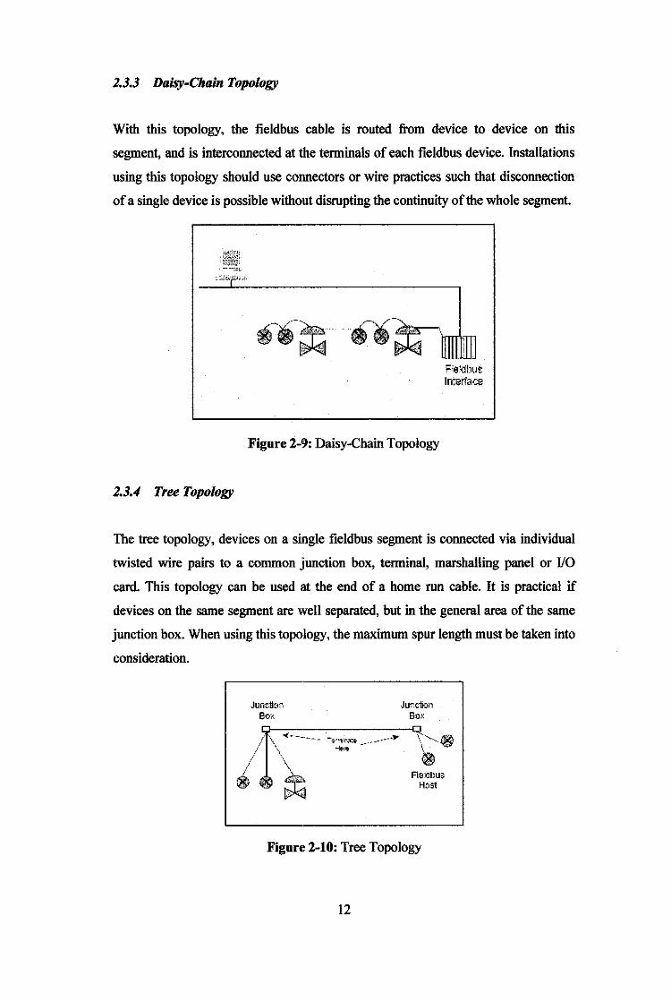
2.3.4 Tree Topology
;:1e/dbus ln:erfao:e
The tree topology, devices on a single fieldbus segment is connected via individual
twisted wire pairs to a common junction box, terminal, marshalling panel or 1/0
card. This topology can be used at the end of a home run cable. It is practical if
devices on the same segment are well separated, but in the general area of the same
junction box. When using this topology, the maximum spur length must be taken into
consideration.
Junc1ior, Bo·r:
Jur.ction Box
Aeklbus Host
Figure 2-10: Tree Topology
12

CHAPTER3
MEmODOLOGY/PROJECT WORK
3.1 Project Work
This chapter is intended to describe the project flow in the development of the test
rig to be used in this project. The following sections introduce the work flow which
could be simplified in a flowchart as shown in Figure 3-1.
Research Work
FYPl Control Loop Design
FYP2 Laboratory Work
Installation & Commissioning
Software & Hardware
Operation & Maintenance
Completion
Figure 3-1: The project flow diagram
13
3.1.1 Research and Information Gathering
The main objective of this project is to build a fieldbus network process loop and this
requires research and literature review to be conducted. Having done the industrial
internship at PETRONAS Carigali Sdn. Bhd. the author obtained valuable
information on fieldbus from major vendors such as Y okogawa, Emerson and
Honeywell. The research scopes include:
• Fieldbus history and the evolution of control system technology
• Fieldbus Foundation defmition, functionality and working its principle
• Installation, commissioning and configuration of the fieldbus system
3.1.2 Control Loop Design
The control loop is to be designed based on the real fire water pump system in a
platform. The system is to be implemented using various field instruments such as
transmitters and valves.
3.1.3 Installation, Commissioning and Confzguration
After the system design is completed and the instruments have been selected, the
device is installed and commissioned with regards to the system manual and based
on the designed schematic.
3.1.4 Troubleshooting, Maintenance and Operation
Several test and calibration need to be done to ensure the connectivity of the fieldbus
system. The operation is remotely monitored, controlled and maintained in real time
application.
14

3.2 Tools Required
The equipments are available as loose instruments n the Process/Instrumentation
Laboratory of Electrical and Electronics Department, UTP. The field devices and
basis components utilized the SMAR Foundation Series 302. Generally, the
hardware and software required to implement a fieldbus system in a segment are:
• Cable
• Terminators
• Power supplies
• Measurement and control devices
• Host devices
• Configuration and operation software
3.2.1 Cable
Various types of cables are useable for fieldbus. The Table 1 contains the type of
cable identified by the IECIISA Physical Layer Standard.
The preferred fieldbus cable is specified in the IECIISA Physical Layer Standard,
Clause 22.7.2 for performance testing, and it is referred to as type "A" fieldbus
cable. This cable will most probably be used in new installations.
Other types of cables are also available to be used for fieldbus wiring. The alternate
preferred fieldbus cable is a multiple, twisted pair cable with an overall shielded
(Type B) fieldbus cable. This cable can be used in both new and retrofit installations
where multiple field buses are mn in the same area if the user's plant.
A less preferred fieldbus cable is a single or multiple, twisted pair cable without any
shield, (type C) fieldbus cable. The least preferred fieldbus cable is a multiple
conductor cable without twisted pairs, but with overall shield (type D). These cables
will mainly used in retrofit applications with limitation in the fieldbus distance. [4]
15

TABLE 1: Fieldbus Cable Types and Maximum Lengths
Type Cable De,;criplion Size Max length
T)1"' A Shielded. ~:.1sted pair #19 A~VG 1900m ~;.:3 mm2; (&232ft.)
Type B Muhi-twisted-1:-'ir <<ilh ohield #22 A\•VG 1200m (.32 tl11112] (3936 ft.]
TypeC Multi-t>·,isted p<lit withoot shield #26AV·lG 400 Ill (.13 tnlll2) (1312ft.]
T'11:oe D Multi-core. •:.1thout t•;,isted jJ<lir·> #16A.~VG 200m and having an O'..-€fal -;.hiekl c;1 . .25 mm2) (656ft.)
3.2.2 Terminal Blocks
Terminal blocks can be the same terminal blocks used in the 4-20mA system. The
terminal blocks typically provide multiple bus connection, such that a device can be
wired to any set of bus terminals.
Figure 3-2 indicates one method of connection and terminating a fieldbus segment to
several field devices at a junction box using the type of terminal blocks that have
been used in the past. Today, there are terminal block systems especially designed
for fieldbus to make wiring considerably easier .
• r u11c1io11 ll<Ox
______________ Shorting Link
:···, I. . Field \\"iring and l"icJ;I Devices
()) ,. I' ' ' ()) I; I -·
I ~· ()) I. ·1 erm ina for
~ 2 l'" . I
()) '-;-~-~- -·-- -~---
' ;_ Q ·- 8!----11; 1 I L_ ()) -...
',L.
/:I ()) T ~·- ()) J '
'------~, ' -- - - j ~horting. Link
Figure 3-2: Terminal Blocks in Field Mounted Junction Box
16

3.2.3 Terminators (BT302)
Figure 3-3: Fieldbus Tenninator
A tenninator is an impedance matching module used at or near each end of a
transmission line. A tenninator is needed at each end of the fieldbus network
segment. The tenninator prevents distortion and signal loss, and are typically
purchased and installed as a preassembled, sealed module. [5] The tenninator has the
following functions:
• Prevent signal reflection
The communication signal bounces back when it reaches the end of the
wire, potentially distorting itself
• Signal current shunt
A device transmits by rapidly changing the current in the network, either
by changing its power consumption or injecting a current. The tenninator
converts the current change produced by a transmitting device into a
voltage change across the entire network that is picked up by all devices
as the means for receiving the signal
17
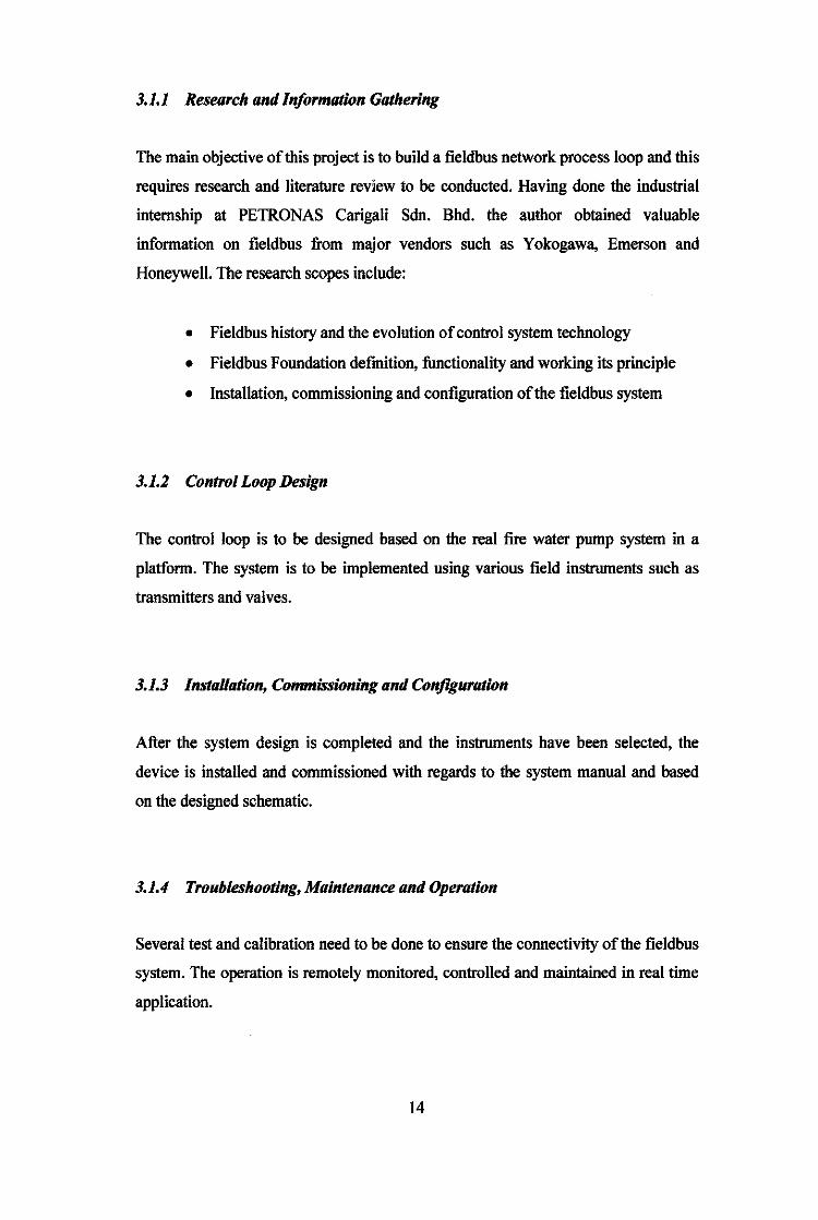
3.2.4 Host devices
Figure 3-4: A Host Computer
A host computer usually a main computer with special integrated software that is
located in the control room that controls the process configuration. Its function is to
manage, monitor, control, maintaining and operate the operation of the control
system made up of devices connected by the fieldbus network. From the fieldbus
network, it can be connected to other computer or other monitoring devices.
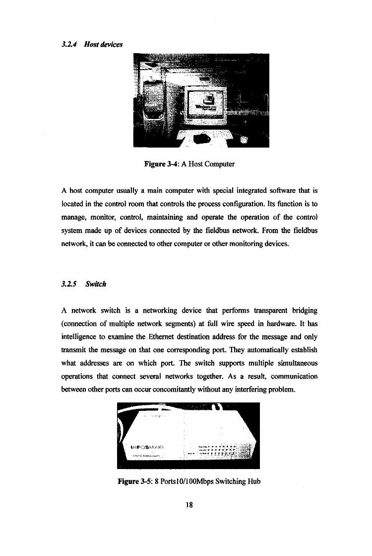
3.2.5 Switch
A network switch is a networking device that performs transparent bridging
(connection of multiple network segments) at full wire speed in hardware. It has
intelligence to examine the Ethernet destination address for the message and only
transmit the message on that one corresponding port. They automatically establish
what addresses are on which port. The switch supports multiple simultaneous
operations that connect several networks together. As a result, communication
between other ports can occur concomitantly without any interfering problem.
Figure 3-5: 8 PortslO/lOOMbps Switching Hub
18

3.2.6 Close and Open Tank
Figure 3-6: Open Tank
The close and open tanks are used in this project to implement the design system that
using both HART and Foundation Fieldbus protocol. Based on the fire water pump
system, the open tank will fill by the standby water while the close tank fills with
water under certain pressure. Both tanks are made by fiber glass material and
attached on the wheels for easy storing and transportable.
Figure 3-7: Close Tank
19

3.2.7 System Conjigurator (SYSCON)
The SYSCON is a software tool especially developed to configure, maintain and
operate the SMAR fieldbus products line, by a Personal Computer with a fieldbus
interface. The software includes the functions:
• System and device configuration
Possible to communicate with all devices in the network, assign tags,
configure the control strategy, adjust parameters and download a
configuration.
• System maintenance
This function communicates with all field instruments and accesses
information about instrument manufacturer, materials of construction and
ranges. It allows for transducer calibration and controller tuning.
• System operation
Indication of variables, historical trends and alarm logs can be retrieve by this
function. The parameters and settings can be changed which is ideal tool for
plant commissioning.
SYSCON • -·-• smar
Figure 3-8: System Configurator (SYSCON)
20

3.2.8 /CONICS GraphWorX32
It is a software solution of OLE for Process Control (OPC) based Client for HMI,
SCADA and control. Object Linking and Embedding (OLE) is a compound
document standard developed by Microsoft Corporation. It enables objects creation
with one application and then link or embeds them in a second application.
Embedded objects retain their original format and links to the application that
created them. OPC is a standard based approach for connecting controllers and 110
devices with HMI client application (e.g. graphics trending). It enhances the
communication of data between device to device and device to host.
Two ICONICS application will be used in this project which is GraphWorx32 and
Contro1Worx32. GraphWorx32 is used to create animated graphics for control
display in host computer. This is where the visualization of the process is created for
the operator interface. Contro1Worx32 is a control application to perform plant
control. [ 6]
Figure 3-9: GraphWorX32
3.2.9 Fieldbus Universal Bridge (DFI-302)
The DFI-302 is a single integrated unit with functions of interfacing, linking device,
bridge, controller, power supply and distributed 110 system (7]. Concisely, DFI-302
is a multifunction hardware component necessary to manage and control the fieldbus
plant. The modules that available in the DFI-302 include:
21

TABLE 2 : DFI-302 Hardware Components
Series Description Specification
DFOI Rack with 4 slots Backplane
DF02 Terminator End terminator for the last rack
DF50 Power supply for Input: 90-264 V AC, Output: 5VDC (backplane
backplane power supply) and 24VDC (external use)
DF51 DFI-302 processor module I x IOMbps Ethernet and 4 x fieldbus HI
channels at 31.25Kbps.
DF52 Power supply for fieldbus Input: 90-264V AC, Output: 24V de
DF53 Power supply impedance To ensure no short-circuit between the power
for fieldbus ( 4 ports) supply and the communication signal on the
fieldbus.
Figure 3-10: Fieldbus Universal Bridge
22

3.2.10 HART Communicator
Figure 3-11: HART Communicator
The HART Communicator is a hand-held interface that used to provide a common
communication link to all HART compatible, microprocessor based instrument.
Calibration of the HART instrument is done using the HART communicator. Tag
name, upper and lower range is set in the HART communicator and sent to the
devices. The HART Communicator interfaces with any HART-compatible device
from any wiring termination point using 4-20 rnA loop, provided a minimum load
resistance of 250 ohms present between the communicator and power supply. It uses
the Bell 202 frequency shift key (FSK) technique of high frequency digital signals
superimposed on a standard transmitter current loop. Because of the total high
frequency signal voltage added to the loop amounts to zero, communication to and
from HART -compatible device does not disturb the 4-20 rnA signal [9].
23

3.2.11 CAJOO Calibrator
In this project, the CA 100 source device is used in order to supply a virtual
temperature to the transmitter. This device is connected to the temperature
transmitter at the same terminal as the output from thermocouple prop is established.
The thermocouple output prop is detached and the temperature source is supplied by
CAlOO to the temperature transmitter.
3.2.12 YSJ36 Yokogawa Controller
A controller can monitor and affect the operational conditions of a system. The
operational conditions are typically referred to as output variables of the system
which can be affected by adjusting certain input variables. For the HART partition,
YS 136 controller is used in order to manage the control valve for the inlet of open
tank (tank 1). The values from pressure transmitter are transferred to the controller
and perform calculation for the valve to react. By using this controller, the
percentage open of control valve can be controlled both automatically and manually.
24

Figure 3-13: Yokogawa controller
3.2.13 URJOOO Recorder
Figure 3-14: Yokogawa recorder
The uRI 000 is a 4 channel paper chart recorder with a II Omm chart span, capable of
measuring voltage, thermocouples and RID's. The recorder is connected at the 4-20
rnA loops and displayed the voltage that represents the level of open tank (open
tank). The trend of the voltage is printed on paper for the history log purposes.
25

3.2.14 Measurement and Control Devices
Below is the list of equipment, measurement and control devices used in the test
platform. The technical specifications for each device are attached in Appendix A.
3.2.14.1 Fieldbus Valve Positioner (FY-302)
Figure 3-15: Control Valve and Valve Positioner
The fieldbus valve positioner offers position sensing without any mechanical
contact, virtually eliminating wear-and-tear and subsequent degradation. The
FY302 directly senses longitudinal or rotary movement based on the Hall Effect.
The position signal may also be used in advanced control schemes. [10]
Features:
• Low air consumption
• Direct, non-contact position sensing
• Valve characteristics change with software cams
• Wide range of function blocks
• Network master capability
26

3.2.14.2 Fieldbus Temperature Transmitter (JT-302)
Figure 3-16: Temperature transmitter
The TT302 fieldbus temperature transmitter provides measurement of
temperature using RIDs or thermocouples and also other sensors with resistance
or m V output. But, in this project the CA 100 calibrator is used to generate a
virtual temperature for the transmitter. A single TT302 model can accept various
sensors, wide ranges, and single-ended or different measurements. It provides an
easy interface between the field and control room. [1 0]
Features:
• Digital LCD display (optional)
• Basic accuracy of0.02%
• Self-diagnostics
• Dual channel
• Universal input accepts several thermocouples, RTDs, mV and Ohm
3.2.14.3 Fieldbus Pressure Transmitter (LD-302 Series)
The LD302 Series fieldbus pressure transmitters are intended for differential,
absolute and gauge pressure; level; and flow measurements. The LD302 Series is
based on a field-proven digital capacitance sensor providing reliable operation
and high performance. The LD302 is part of SMAR's complete series of fieldbus
devices. [10]
27

Features:
• 0-125 Pa to 0-40 Mpa
• 0.075% accuracy of calibrated range
• Accepts range from URL to URL/120
• Wetted parts in 316 SS, Hastelloy and Tantalum
• Self-diagnostics
Figure 3-17: Differential Pressure Transmitter
Figure 3-18: Gauge Pressure Transmitter
28

CHAPTER4
PROCESS PLANT AND CONTROL STRATEGIES
4.1 Petrobras Platform P-36 Explosion, Brazil
Figure 4-1: Platform P-36 Location
The Petrobras Platform 36 (P-36) was located in the deepwater Roncador Field in the
northern Campos Basin area, some 125 km off the coast of Brazil. Campos Basin is
the largest oil reserve in Brazil, covering an area of over 100,000 km2 and was
discovered in 1976. The Roncador Field, discovered in 1996, covers an area of 111
km2 and has a sea depth varying from 1,500 to 1,900 m.
The P-36 was transformed from a drilling rig, known as Spirit of Columbus, into a
floating production facility with a processing capacity of 180,000 barrels per day. It
was a moderately sized semi-submersible platform with two submerged pontoons
supporting four large columns which in turn supported the main deck housing the
production facility.
29

As typical for semi-submersible platforms, the P-36 was floating on the sea by
buoyancy and had no physical support to the seabed. It was positioned on the surface
of the sea by an anchoring system. The P-36 had been in production since May 2000
and had an oil production rate of around 80,000 barrels at the time [II].
4.1.1 The explosion and fire
In the first hour of 15 March 2001, three explosions occurred in the starboard aft
column of the Petrobras Platform P-36, causing the fire and flooding of the platform.
The platform sank into the water of approximately 1360 m deep on 20 March 200 I.
The incident was initiated by the rupture of the Emergency Drain Tank (EDT) in the
starboard aft column due to excessive pressure at 00:22 on 15 March 2001. The
rupture caused damage to various equipment and installations, leading to the
flooding of water, oil and gas into the column. Emergency Firefighting Service was
sent to the area. After 17 minutes, the dispersed gas caused fire, causing a major
explosion which II crews been killed in the incident. The explosion also resulted in
serious physical damage to the platform.
Of the 175 people on board, 165 were successfully evacuated including a person who
was seriously burned and died I week later. The continuous flooding fmally
destabilised the P-36 and it sank five days later.
Figure 4-2: Platform P-36 after explosion
Source: http://www.mace.manchester.ac.uk/
30

4.2 Fire Water Pump Control System
r----l--------------------- -----------,
r .. u
;_ _______________ --------------------- ---- _ _;
------------------,
Tuk2
.. \ I
~./
Figure 4-3: P&ID of process loop design
Triggered with the safety system on a plant, the control loop design is based on the
fire water pump system. Referring to the Figure 4-3, the control process consists of2
tanks; one is an open tank while the other one is a close tank. The design is based on
availability of devices in the laboratory. This process loop consists of all instrument
devices such as control valve, level transmitter and pressure transmitter.
The constraint of the Fieldbus devices resulted to the use of HART protocol in the
control loop design. The HART protocol is used for tank I while for the tank 2 it is
fully foundation fieldbus equipped. Instead of using the Foundation Fieldbus
protocol, the combination of HART protocol fulfills a part of this project objective to
show the advantages of the Foundation Fieldbus in term of robustness, better
controllability, saving cost and compatibility with other system.
31

When designing a process loop, we need to consider eight (8) criteria of control
objectives in order to place the controller and transmitter, and they are:
• Safety
• Enviromnental protection
• Equipment protection
• Smooth operation
• Production quality
• Profit
• Monitoring and diagnosis
In Figure 4-3, the location of the pressure and level transmitter has been specified
based on the requirement of the control objective. The level controller at tank 1 for
example ensures the safety and smooth operation of the process. It prevents the tank
to overflow by controlling the inlet flow to the tank and at the same time maintaining
the level for use in the next process.
4.3 HART - what is it?
Devices using HART communication technology hit the market early 1980s. The
HART Communication Foundation estimated that there are 10 million HART
devices in service throughout the world today. [3]
In HART devices, data are delivered via digital signaling "superimposed" on top of
the traditional 4-20 rnA current loop used to return (or send) the process variable
(PV). The communication speed for HART signaling is 1.2 Kbps. With HART
devices, the PV is always being derived from the 4-20 rnA signals despite the fact
that the PV is also available as part of the digital data provided by the device. In fact,
many HART devices installed today still use the PV and ignore the digital data
provided by the HART protocol. On the other hand, HART protocol does not allow
several devices to be connected in series in the same current loop, thus providing
digital data from each device.
32

Table 3: Characteristics of HART and Foundation Fieldbus
Characteristic HART Foundation Fieldbus
Uses 4-20 rnA for providing PV Yes No
Data provided via digital signaling Yes Yes
Type of communication Master I Slave Token passing
Bus speed 1200 bps 31,25 kbps
Remote configuration I calibration Yes Yes
Provides device diagnostics Yes Yes
Multi-drop confignrations Yes (limited) Yes
Approximate number of devices in service 10,000,000 300,000
Suitable for intrinsically safe application Yes Yes
Non-proprietary I vendor neutral Yes Yes
Supports control in the field No Yes
Similar 1/0 interfaces would connect the HART loops and the fieldbus segments to
the control system computer. In such confignration, it would be typical for the
fieldbus 1/0 interface to connect to multiple multidrop fieldbus segment with multi
devices on each segment. The HART 1/0 would typically be wired so each HART
device connects to a separate channel on the HART 1/0 interface.
'<& : li-JOl
- Product -
A slnopl<> <a«ad<! <ontrolloop shows lhe FT101 and FCV101 are ftekfbus fmctfoo blocks IO<ated In fteldoos devkes FT-101 and FCV-101, respectively. TT100 and TIC100 are non-fleldoos functiOn blod<s ltxatOO In the control system PC. TT~tOtlsa HART device providing the Input to the TT100 At fum:uon block. 1be trick Is for the control system to COI'M!rt the ou1pUt of the convooUonal nctoo funcuon block Into • fleldoos output. so It <an p<oVIde a cascade-Input to the FIC101 fleldbus tuncuon block contained In fleldbus devke FT101.
Figure 4-4: HART and fieldbus control system
33

The design of the process control is based on the actual process of frrewater pump
system. This system mainly designed for the plant as the fire fighting system where
the operation needs to be l 00% accurately functions, as the environment is
hazardous and flammable.
This process loop consists of two tanks where the open tank reacts as a standby water
tank while the close tank mainly operates during the processing of the system. All
the instrument devices react to the situation for the smooth process of the system.
The algorithm of this process loop requires a set point is place for the level of tank l,
the open tank. Water from the supply fills up the open tank until reaching the set
point. This inlet flow is controlled by the control valve, based on the reading of the
level transmitter value. If it is below the set point, valve will be opened and fill up
the tank. If it reached the set point, the valve will be closed. For the safety reason, an
overflow outlet will be places at the most top of the tank.
A pump and a foundation fieldbus control valve is attached at the outlet of the open
tank which is connected to the close tank, tank 2. The outlet flow of the tank l will
be controlled by the control valve based on the reading from the pressure sensor at
the close tank. Water fills up the close tank until it reaches a certain value of pressure
that is set by the user. If the pressure drops below the set point, the valve will be
opened and water flows into the tank. If the pressure achieves the set point, the valve
will be closed and stop water from flowing into the tank. To make sure that the water
in tank 2 is not overflowed, the system is enhanced by introducing a level
transmitter. The control valve to tank 2 reacts not only to the pressure but also the
level of tank 2.
In the real application, the outlet of the close tank will be attached to the sprinkler
However, in this project it is replaced by the shower where the flow is controlled by
the hand valve due to budget constrain. Although this design used the HART
protocol, but for the critical loop the Foundation Fieldbus protocol is the choice.
34

4.4 Control Strategy Design and Configuration
The process loop has numerous inputs and outputs that will be used to provide
information for the next process (see Figure 4-5). All the inputs and outputs signals
are important in order to have the desired product that is maintaining the pressure of
a close tank at a certain set point.
1-.Iauipillated lllput PROCESS
£]f;;; Ou.iPi.\t r-s '.
~ Di>lutba,ce Input> -- .:.:.
Figure 4-5: Diagram of a certain process
The inputs can be generally:
• Disturbances.
Disturbances are variables that fluctuate and cause the process output to
move from the desired operating value (setpoint). A disturbance could be a
change in flow, temperature of the surroundings, pressure etc. Disturbance
variables (DV's) can normally be further classified in terms of measured or
unmeasured signals.
• The manipulated variable (MV).
This is the variable chosen to affect control over an output variable. As the
output is being controlled it is normally referred to as the controlled variable
(CV). On a typical chemical process there are generally many CV's and
MY's.
The objective of a control system is to keep the CV' s at their desired values (or
setpoints). This is achieved by manipulating the MY's using a control algorithm.
35

4.4.1 PJD Controller
A proportional-integral-derivative controller (PID controller) is a common feedback
loop component in industrial control systems. The controller compares a measured
value from a process with a reference setpoint value. The difference or "error" signal
is then being processed to calculate a new value for a manipulated process input. The
new value takes the process measurements value back to its desired setpoint. Unlike
the simpler control algorithms, the PID controller can adjust process inputs based on
the history and rate of change of the error signal, which gives more accurate and
stable control.
A control loop consists of three parts:
1. Measurement by a sensor connected to the process,
2. Decision in a controller element,
3. Action through an output device ("actuator") such as a control valve.
' . SE·T!I'Ol~f······ ...................... ·-~~N~e~~ .. , : PID : ~ DIFfERENCE ......,. ERROR ) CONTROL ~ ~ l ALGORITIIM 1 '·········· ···················································.··t .. ··········'
OUTPUT
PROCESS L~ VARIABLE :::1~.:]
Figure 4-6: PID controller
The controller reads a sensor, subtracts this measurement from a desired value i.e.,
the "setpoint" and determines an "error". It then uses the error to calculate a
correction to the process's input variable so that the correction will remove error
from the process's output measurement. It then adds the correction to the process's
input variable to remove errors from the process's output.
36

-----··-----·--·--·----··-··-·-----·--·--,
Tukl
~-- --------- ----- ·-··--·-··---
-------- ---------------·------ ---------------- ·---·- . -,
0, r
Taok2
Feudati .. :Fid6w: Plo1Nel
Figure 4-7: PID controller with feedback loop
In this project, when using the feedback control loop with PID controller, the
opening of the control valve is controlled by the amount of the pressure in the tank.
For a given set point, if the pressure drops below the set point, the valve will be
opened to fill up the tank and vice versa. For example, the decreasing of the pressure
of tank 2 will increase the opening of the valve of the inlet of close tank to maintain
the desired pressure.
The same reasoning goes to the level controller. When the water of tank l reaches
the set point, the control valve at the feed will be closed in order to prevent more
feed going to the tank. If the level drops below the set point, it will give a feedback
signal to the controller and give order to the valve whether to open wider, or smaller.
This process will be repeated until the set point is achieved.
37

4.4.2 Feedforward Control
Feedforward differ from the feedback. Feedforward uses the measurement of an
input disturbance to the plant as additional information for enhancing single-loop
PID control performance [1]. This measurement provides an "early warning" that the
control variables will be upset some time in the future. With this warning, the
feedforward controller has opportunity to adjust the manipulated variable before the
controlled variable deviates from its set point.
r------------------ ------------------ -----,
Toakl
;__ ___ ------ ---------------------------- ---- __ .,; F......_,.._Pa-.J.
r r 0-----------------·---- --·-0·-- -----·---·-·-----·--- -n
Figure 4-8: Feedforward Control
Applying feedforward requires an additional temperature controller to be attached at
the output of tank 2. Both outputs of temperature and pressure controller will be the
set point to control the opening and closing of the inlet control valve of tank 2 (see
Figure 4-8). What actually happen in this control design is that when there is a frre
and which result the increasing of temperature and will be sensed by the temperature
controller. Before the pressure drop due to the water goes sprinkler in this case the
opening of hand valve, the output from the temperature sensor will send signal to the
controller to give early warning to the valve to open. In this case, the pressure would
drop slightly lower compared if there is the feedback loop alone. This will enhance
the control ability of the controller.
38

4.4.3 Ratio Control
Ratio control differs from the feedback. Ratio control is used to ensure that two or
more flows are kept at the same ratio even if the flows are changing. [I] For this
project, ratio control is used for measuring the ratio of pressure and flow in order to
enhance single-loop PID control performance. In this control strategy, the pressure is
set at a certain value. The amount of inlet flow of tank 2 will be control by the ratio
controller. After the pressure has achieved the set point, the valve will be closed and
no more flow to tank 2.
----- ------------- ------------ --------------- --------~
··-··-··-··-··-··- ·-·--··- -··------------, .----~ --·-------- ------------·----------:
Figure 4-9: Ratio Control
Applying ratio control needs to have a flow controller to be attached with the
pressure transmitter of tank 2. Both the outputs of flow and pressure controller will
be the set point to control the opening and closing of the inlet control valve of tank 2,
depending on the certain amount of ratio (see Figure 4-9).
39

4.4.4 Cascade Control
Cascade control is one of the most successful methods for enhancing single-loop
control performance. In cascade control, the output of the primary loop will be the
set point for the secondary loop. Referring to the Figure 4-10, the temperature
controller is the primary while the flow controller is the secondary. The output of the
temperature controller will be the set point of the flow controller, the secondary. [1]
Process Fluid
Steam Va~e
Steam
I
~ ~1c Temperature ----tili;t'----- "' Controller Flow Controller (primary)
{secondary) :
Shell and Tube Heat Exchanger
Temperature Measurement
Figure 4-10: Cascade Control
Reasons for cascade control include:
• Allow faster secondary controller to handle disturbances in the secondary
loop.
• Allow secondary controller to handle non-linear valve and other final control
element problems.
• Allow operator to directly control secondary loop during certain modes of
operation (such as startup).
Requirements for cascade control:
• Secondary loop process dynamics must be at least four times as fast as
primary loop process dynamics.
• Secondary loop must have influence over the primary loop.
• Secondary loop must be measured and controllable.
40

r---------- --- - ·-- - .. - -- ·-·- ---- ·-,
Tukl
i ---------- -------,
'I, ~'"' 1:\1 ,----------·--·--· -----1 pe' .\
. 'j .•·
Tuk2
Figure 4-11: Cascade Control in the process design
Figure 4-11 shows the arrangement where the level controller is the primary loop and
the pressure controller is the secondary loop. The output from the level controller
will be the set point to the pressure controller. In this case, instead of using single
loop only, having both pressure and level measurement will increase the control
performance of the system. The advantage of having the level controller is if there is
any leakage in the close tank, the water level will not exceed the limit because the
priority is set to the level rather than pressure itself.
In tbe first draft design, a flow transmitter will be put at the inlet of tank 2 and be
cascaded with tbe pressure controller. But, as been informed by the lab technician,
there is no spare part of orifice plat that can be use in this project. Due to this
problem, the design has been changed by using the level controller.
41

CHAPTERS
INSTALLATION AND COMMISSIONING
5.1 Decommissioning Existing Plant
In this project, older plants were upgraded with the fieldbus system. The plant
consists of two tanks; open and close tank. Both tanks were used for demonstrating
the level measurement using the conventional instrument devices. All the transmitter
and control valve need to be decommissioning in order to suit our foundation
fieldbus instruments. Some of the existing tubes and pipes are being reused as this
project requires the level controller strategies for both tanks.
Figure 5-1: Decommissioning process
42

5.2 Painting Process
The trolleys that support both tanks are rusty due to the effect of corrosion. Because
of that, the tanks are painted with oil base painting which is red-orange in color same
as the function of fire water pump system. The painting process become easier as all
devices have been detach from the plant.
Figure 5-2: Painted Platform
5.3 Hardware and Piping Installation
Figure 5-3: Piping and hardware installation
43

In this project two tanks, two control valves, three differential pressure transmitter,
two pumps and two hand valves need to be connected to imitate a fire water pump
system. The pipe that has been used is the galvanic type. For the manifold, 1 Omm
cuprum tubing was used together with the joints. The tubing is connected from the
differential pressure transmitter to the tank and familiarization of bending technique
during the internship is useful throughout the commissioning of all instrument
devices.
5.4 Network Installation
This project used both HART and foundation fieldbus protocol of network
communication. For the fieldbus network it has two wires used for both
communication and power supply. The devices are connected in parallel, thus it is
possible to connect or remove device while the bus is running. Each segment of the
fieldbus network has to have two terminators, one in each end. In this network, the
power supply, host end terminator and host interface have been integrated into a
single device, DFI-302 to simplifY wiring in the panel. There are two methods in
supplying power to the devices; bus powered and non bus-powered. Bus-powered
devices take power from the bus. The non bus-powered devices get power over
separates wire. For the HART network, the measuring device is supplied by external
power source while for the final element such as control valve, the signal is produced
by the controller itself.
5.4.1 Establishing Loop Connections for HART Network Wiring
The controller, recorder, power supply, temperature transmitter, control valve, 2500
resistance decade box and differential pressure transmitter are used in establishing
the loop connections. To establish the HART connection loop, the wiring steps to be
conducted are:
44

i. The positive and negative terminal of the differential pressure transmitter
is connected with a wire as shown in Figure 5-4
Figure S-4: Wiring connection at the differential pressure transmitter
ii. At the power supply (Figure 5-5), the ground terminal (white jumper) is
connected to the ground terminal of the controller. The positive supply
(red wire) is connected to the positive terminal of the differential pressure
transmitter.
Figure 5-5: Wiring connection at the power supply
iii. Figure 5-6 shows the connections made at the controller. Terminals 1 and
2 (in red shape) are the positive and negative terminals for Process
Variable (PV) input, respectively. The range of input is to be between 1 to
5 V de. The blue shape highlights the terminals 22 and 23, which
represent the positive and negative terminals of manipulated variable
(MV) output 1, respectively. The output range is in between 4 to 20 rnA.
45

Figure 5-6: Connections at the controller (backside)
The positive tenninal of the PV input is connected to the ground tenninal of
the differential pressure transmitter (yellow jumper). The other connection
(white jumper) for the positive tenninal comes from the ground tenninal of
the resistance decade box. For the negative tenninal, it is connected to the
ground tenninals of the resistance box (green jumper) and power supply (red
jumper). The wiring from MV output is connected to the positioner valve as
shown in Figure 5-7.
Figure 5-7: Wiring from controller into the control valve
46

iv. Figure 5-8 shows the connections at the backside of the recorder. Input
terminal of channel I is used, as circled by the white and red oval in the
figure.
Figure 5-8 Connections at the recorder (backside)
The positive terminal (green jumper) and negative terminal (yellow
jumper) is connected to the positive and negative terminal of the
resistance decade box, respectively. With these connections, the positive
terminal of the recorder is also connected to ground terminal of the
transmitter and negative terminal is connected to the ground terminal of
the power supply.
v. Figure 5-9 shows the connections at the decade box.
Ground terminal: Controller ground (green) Recorder ground (yellow)
Positive terminal: Controller positive (white) Recorder positive (green)
Figure 5-9 Connections at 2500 Resistance Decade Box
47

vi. The complete connections described for HART network can be
represented into loop drawing as Figure 5-l 0.
Transmitter
[>N PrlOO
r+Fl TIP Valve ~20psi
~ Power Supply
l§"'•' rr 4-20mA
t: r--
COillroller Recorder
~ ~ ~: f. 4-20mA 2500hm
PIC 100 Resistance
Figure 5-10: Loop drawing designed for HART network
5.4.2 Foundation Fieldbus Network Wiring
The test platform of fire water pump comes with Daisy-Chain topology as shown in
Figure 5-11. This fieldbus topology applies end-type terminator for the following
reasons. The primary function of the tenninator is to convert the transmit current to a
voltage that can be received. According to the standard, the current must be
modulated with amplitude between ±7.5 rnA AC to ±10 rnA AC (Smar is using
±8mA). When the fieldbus signal traveling down the wire reaches the end, it is faced
with a change in impedance from the characteristic impedance of the wire to the
infinite impedance of open air. This will cause a part of the signal power to be
reflected back up through the wire. The reflected signal interferes with the oncoming
"real" signal. If the reflected signal is powerful enough, it may distort the "real"
signal such that the communication does not work. The terminator has the same
impedance as the cable such that when placed at the end the fieldbus signal sees no
change in impedance and hence there is no reflection. It is also clear that the
terminator must be at the end of the wire to really work.
48

Sate Area
Host Computer llr'"--rl
Hub
Fleldbuo Universal Bridge (DFI-302)
Hazardous Area
F'i-302
L0-302 (L2:1
LD-302 L0-:02 (M4) (02)
Figure 5-11: Daisy-Chain Topology
To establish the fieldbus topology, the wiring steps to be conducted are:
i. The Electrical Connection Cover is released by rotating the cover anti
clockwise. Signal wires must be kept separate from sources and noise.
Because of the polarized signal and bus-powered devices the polarity of the
connection must be under consideration. The devices are all connected in
parallel, thus colour-coded crimp is used to unite all negative terminal in
same node and all positive terminal in the other node.
Figure 5-12: Colour-coded crimp
49

ii. Using the Daisy-Chain topology needs the cable to be connected from device
to device meaning that the possibility if a device disconnected and interrupted
other device are high. Therefore the same conduit for "in" and "out" wires is
used in order to enable removal of device without disconnecting entire bus
(see Figure 5-13).
Figure 5-13: Daisy-Chain Wiring
Figure 5-14: Daisy-Chain Topology Implementation
50
CHAPTER6
SYSTEM CONFIGURATION AND INTERFACING
6.1 Foundation Fieldbus Configuration
In the fieldbus system, it requires the engineer to configure the network and also the
control strategies together with the devices. This objective is achieved by using the
SYSCON (System Configurator) which is a software tool developed to configure,
maintain and operate especially for the SMAR Fieldbus products line, using a
personal computer (PC) as a host with a Fieldbus interface.
The configuration process starts by creating a file for the workspace. It can be
divided into two parts; The Logical Plant and the Physical Plant. In the logical plant
where the logic part of the system is kept such as the connection function blocks
while for the physical plant, the configuration of the fieldbus network been made for
all field devices installed in the segment. Then the configuration of the field device
and control strategies can be established by initializing the communication between
devices and host PC, uploading the fieldbus network, commissioning the device,
design the control strategies in function block and downloaded back the
configuration in the devices.
,+8 Tes!Piri :+; 0 lo<;;tal ~ ~~ ... ~.11111@1
Figure 6-1: SYSCON Main Window
51

6.1.1 Initializing Device Communication
The initialization of device communication is significant for the SYSCON to detect
the fieldbus network. Below are the steps taken to initialize the online
communication:
i. The communication setting is selected in the popup menu activated by
right clicking Fieldbus Network icon as the following figure.
fiR Syscon - new
Project File Edit Search View Comnuication Window Help . '~ ---- --- -----· - - -
ii. The server ID is set to Smar.DFIOLEServer.O in the communication
setting dialog box.
Commumcat10n Setting§ ):'!
r;,, : ,,,. :-Smver Context-
!) : r lnpr~ r Local
Node Name:
jThioNode
OK c.ncel
iii. The ON Button in the toolbar is clicked.
Project Ale Edt
52

iv. The communication initializing window will popup and the bridges
installed in the computer is attached to the configuration software.
Imt Communication-...,.
Elapsed Tine: illifOO Abort
6.1.2 Uploading Fieldbus Networks and Devices
The online communication has been initialized in the previous part. The device
topology and device list is needed to be uploaded for the configuration process.
Below are the procedures to upload the device to the Physical Plant.
i. The Fieldbus Network is right clicked in order to activate the popup
menu. The Upload icon is selected in order to upload the devices list into
the network
Syscon new
ii. After the Upload-Fieldbus Network box appeared, the Topology and
Device List is checked in the filters selection before the Start button is
pressed.
53

"" (;)--._-------, L_ ----~~~---· .
D.~ .. ~in~'-'-" .
' ~-~~-ill-~-~·-:·
.
"" ' r Bb:kUct "" i I Par-*
~-~in~_-·
"" j Nelwolk: Nwrtler.
: Device: AdcRa:
I \IF[): Refeftlnce:
0~ ODindelt
, ... -iii. The Fieldbus I icon is double clicked to open the network that being
used. In the Fieldbus 1 window, the popup menu is activated and Live
List is selected.
~" 15!, TestPI<ri :+; () LO(jcal Plant ~, !!!® Reldbus
'~ 'is DF!302 ;s;-_j[]j.!!J
iv. This window will popup and show each devices address and its unique
device identifier ID
54
(QlX120115~1i'IJI OxiS
!Kim2!mltSMNHim2:!nllni1QJ OX18
!IIXl3020Xlli:SMAR-ff.m:~ Ox!A tm.1121m2:SMNH13)2:oomi910 tbf4
000'3021Dll:Sr!WHD30Z:Wllnm7 OxF5 IOIJI2IDII:SMAA-1.0002:1m117001 OxFi'

6.2 Device Commissioning
One of the advantages using Foundation Fieldbus is the device can be easily
commissioned from the control room. The DFI-302 is automatically assigned node
address assignment for each device.
6.1.1 Changing Device Attribute
The attributes for each device are unique and assigned by the manufacturer in order
to ovoid network conflict. This unique attribute serves the foundation fieldbus to be
interoperability where devices from other manufacturer can work together in the
same network connection. Below are the procedures to change the device attribute:
i. The popup menu is activated by right clicked on any device in the
Fieldbus window and attribute is selected from the list
Projett""' &It SNrd> ~ v.w... Hat>
~. III_J_Jfil .il~L!J
~~-c; .... "- !!fi fllllr.t... Noblod<s
~-·Brllbol lr": AodMI ~- Fioklus2 ~ Flelclu3 G.:":FielcbJsol
-~:~
:""liE • A~ . "''" • rr.., • Pl"-o21 + n-w
........
....,.r~~g.,.
""""''""" -· """"""·· -.. . , ..
ii. The Device Attribute box is appeared. Only Device Tag is allowed to be
changed by the user due to the product line and network conflict
protection taken by manufacturer.
OK
55
"•• I I '

6.2.2 Creating the Function Block
By linking several function blocks, various control strategies can be implemented in
tbe fieldbus network. A device is allowing the selection up to 20 function block per
device. Below are the steps to add blocks for a device.
i. To add a new block, the popup window is activated with tbe right mouse
button at the FB VFD. The icon new block is selected as seen in the
following picture.
Ei ®;?, Reldbus!
"' lis Df!302 -"i ~ Temperature
. --~ MIB
.• !-~ ! ~ ::.:~ -=L&~ .. -·~ ~ fl-302 +J ~ PT-!121
ii. The new block windows will popup. The block type is selected from the
menu and tagged using preferred name.
o-· ;.;_~fllill:u~
~~ l1a Bridget w., Aekhusl ~; Fiollba2 5:!,Flrilkbus3 ~l'lekbu<4
NonJocU<r: ,-----------,
Devic&TJIIIII: ,----------,
DoMcefle-.: r-=J DDRiw.: r---:J CFRev.: r--::J Bloci:TJIIIII: )AMili!ilrW ::J Pnfie: ~----
91Ddr.Tag: O,~niN.....,-,---------
56

6.3 Creating the Control Strategies
The control strategies to be implemented in this project are created and configured in
the logical plant area window. Two control strategies have been combined together
to individually control the process of heat exchanger. The control strategies involved
are:
a. Single loop feedback control
b. Feed forward and feedback control
i. New Process Cell is created under the Logical Plant by activated the
shortcut menu with the right mouse button. New process cell tab is
selected and Process Area window is appeared.
Syscon nt:w
-"' Edt """"' ........ """ - - -----~
ii. In the Process Area window, the shortcut menu is again activated with the
right click mouse button. The New Control Module tab is selected to
create a control strategy.
-~-o Areat
~~>--'-: 1\!e l'ielcbs-"' --' <;1jglll'lcbol
~ Flekb.lst ®;'". Aeki:us2 <57,, Fieldbus3 ~l'ieldb<wf
57

iii. The Control Module windows will popup and the tag for each control
strategy can be created
new +()Areal ~ Process Area
_, li!® Fieldbus Networl<s C' ~Bridge!
:g Fieldbusl
'""' Fieldbus2 ®A Fielcbus3 ®?; Reldbus4
Control Module ~',.
Tag:
jfeediO!Wald
OK Help
iv. The specific control module is clicked to open the working area. Three
windows are opened together as shown in figure below. The desired
block is dragged from the Bridge l window to the Process Area and to the
desired Control Module window. All the blocks are connected with the
link icon according to the control strategies designed.
'"'" +, 0 TlJDZ_.RS _+c (], Tt30ZJR :0' 0 TT3Il2_DSP .. : [1 TTIOO_AI +• 0. T!CIOOJ'IOC +: 0 TIC2llll_PID5 .. - 0 T!C'lOO_PIDF
.@ ...
. :: • Conbd ..,.,.,
l\li]"" - lil fB¥fl)
+: 01'Y3112JG +_ 0 FY302_m .. _ 0 FY30Z...PSP +; Q FCVIOO.JIO .• ~"''"-"'
·.: Ff.:30Z +: PT.ml
i.cnu;w;;rm ,,.., ... ,!1'-...
-- Ul!le loop +: 0 TIC200_PID5 +- [l TTIOO_AI
+ 0 FCVJOO_AO •· Q FVIOO..,sa
..- 1§1 F :l J aacfu-d
58
1-·.'
:.!.1 l,.,lvl•l''.;;
~---------------~ I I
I
I
I
I
I
I
.,
j
'"'"'

6.3.1 Single Loop Feedback Control Function Block
----------------------------------- --- ------------., ·--------------~
"·-·- .. ·--- - - ' i '
Tukl
Figure 6-2: P&ID of Single Loop Feedback Control
Feedback control strategy is one of the process control used in this project. The
disadvantage of this control strategy it is only depending on a single transmitter to
provide the response back to the controller valve. This control scheme involve only
pressure transmitter and control valve and does not take into consideration of any
other process variable.
tY
Figure 6-3: Function Block of Single Loop Feedback Control
59

6.3.2 Feedforward Control Function Block
?~ ~ ~ ~ ~ ~ ~ ~ ~'" ~ ~ ~ ~ ~ ~ ~ ~-?
;';
-:Jc.~
: u··.l_ -: : ~. I
·~-~- "' :
Tod<l
J«llTI'm11cel Foaobliu F"•Wilu:s Pn.tocel
' ' .:-- - - - - - ·- - - •:> - - - --- - - - -o
Figure 6-4: P&ID ofFeedforward Control
In feed forward control, an input disturbance is measured to determine an adjustment
to an input manipulated variable before the controlled variables deviates from its set
point. In this project, the temperature sensor giving the early warning to the system
that a frre might occur and the pressure of tank I will drop as the fire fighting is
operated. However, feedforward control alone cannot eliminate the steady state
offset. Hence, feedforward is combined with feedback control as each has important
advantages that compensate for deficiencies of the other. The major advantage of
feedback control is that it reduces steady-state zero offset to zero for all disturbances.
(------ ---------- ~
/n1011Jt1\
\~-.J
'
Figure 6-5: Function Block of Single Loop Feedback Control
60

CHAPTER7
FIELD BUS SAVINGS AND BENEFITS
7.1 Data Quality and Quantity
7.1.1 Increase quality of product
More accurate values I more information PLC 1 ocs
l:i:~ lZ'!Ii
fdentlflc:itlon tog: softw-~n: 9ell.:~l n~mbtr: elc ......
- Pr012 -1.1 • 4M6l'l237
1st process value -1o.n 2ndproa.S'9 valuot • 23.02 Engineering lllllt • mbi!r SWus-Oualltv •OK
Figure 7-1: HART and Fieldbus Data Transfer
Figure 7-1 illustrates the HART and foundation fieldbus data transferring from the
field device to the PLC or DCS. Looking to the HART signal, there are 3 times
conversion from AID or D/A before reaching the controller. These phenomena will
increase the distortion of the signal making the signal less accurate and result to the
decrease of data quality. Having the inaccurate data to be processed in the
controller will result the fmal element to react inefficiently to the process loop. As
the conclusion, the product produce will less quality and decrease the profit of the
company.
61

Different from using the foundation fieldbus technology, it has increased the
resolution and less distortion of the data transferred due to reducing of data
conversion. The data or measurement from the fieldbus device is higher in term of
accuracy taking the advantage of digital signaling. This will result to the increasing
of product quality and at the same time rising the productivity owing to the precise
data that been processed in the controller.
Figure 7-2: Online Configuring
As shown in figure 7-2, the entire configuration of this project is done online for the
foundation fieldbus while for the HART portion it is all done in the field. It is much
easier to calibrate the device in the control room rather to go to the plant. This is due
to the benefit of using the digital communication network where many data can be
transferred not only the measurement values but also for configuration purposes.
62

7.2 Decrease Total Cost
7.2.1 Hardware reduction
DISTRIBUTION OF FUNCTIONS
a ~
I1 • Flt!ldbus can be used in the same way.
In today's systems, control functions but fieldt»Js also enables control and 110 all reside in central controllers. funCUOns to be dlsbibUted to field
lMtrumenm.
Figure 7-3: Conventional and Fieldbus Control Loop
As shown in Figure 7-3, sensors and actuators for the conventional control loop were
hardwired to the controller using an individual dedicated pair of wire. For the
foundation fieldbus control loop, each device can be attach to the bus and result to
the hardwire reduction.
In term of the IS barrier used in the control loop, using the conventional control
system each segment need to be attach with IS but for foundation fieldbus
technology, IS barrier is only used at the line before connecting to the controller.
Figure 7-3 points up the shift of control system functions to the field level. Such
implementation reduces the 110 cards and control equipment needed such as card
files, cabinet and power supply.
As shown in Table 4 is the cost comparison between conventional control loop and
foundation fieldbus protocol. Although the transmitter and the valve for the
foundation fieldbus is much higher, but by using fieldbus 30% of the total cost of
this project can be reduced. The wiring for fieldbus is lower compared to the
conventional system and by using the foundation fieldbus protocol less device is
needed to complete this project.
63

Figure 7-4: Wiring connection using HART
Figure 7-5: Wiring connection using Foundation Fieldbus
TABLE 4: Cost Estimation for Conventional and Fieldbus System
Conventional~ Fieldbus (RM) Power Supply 200 120 Interface 280 640 Wiring and Fittings 5 600 1160 Valve 2260 4100 Transmitter 2200 2500 Standalone PC NA 3 000 Hub NA 500 Terminator NA 200 Controller 2 100 NA Recorder 2 900 NA Decade Box 1500 NA Labor Cost 2040 1400 TOTAL 19080 13620
64

7.1.1 Maintenance cost reduction
Data trending
Diagnostics Applications
' 1l lmpu~lu~BI«kmgDill'!o;ti«l
1) t<rea R~Mih.4ing
~"'-...... --•-...,; :.·. ·. ... l) T«i!l tldlffi\ Not- .tU 'f<!IIR~ '';"" .. 41 HlilQ..,.~tw
' --~-------- .. ·---
Figure 7-6: Diagnostics capability
Successful process automation is enabling refiners to increase productivity, improve
asset utilization and increase tbe qnality of tbe product. Using the conventional
control system only provides tbe information of control variables but by using
foundation fieldbus more data can be transferred because of the digital
communication system.
The foundation fieldbus devices have tbe self diagnostic capability and will alert the
operator if the device needs to be replacing at a certain time. This prediction
maintenance feature allowed tbe operator to search for spar or stocks. Using the
maintenance software can reduce tbe maintenance cost because all tbe maintenance
activities can be done in the control room instead to be checked in the field
manually.
65

CHAPTERS
CONCLUSIONS AND RECOMMENDATIONS
8.1 Conclusion
This project is focusing on the implementation of the foundation fieldbus
technology. Foundation Fieldbus is an all-digital, bi-directional, multidrop, serial
bus, communications system that serve as the base-level sophisticated network for
plant or factory automation enviromnent. Fieldbus technology is already changing
the way systems performs control. Some users have gone toward using fieldbus in
their plant, whereas others have implemented a full scale fieldbus system. In oil and
gas industry, many companies in the world including PETRONAS have
implemented fieldbus foundation in their designs. It has been stipulated that the
fieldbus has credibility over DCS in terms of hardware installation, wiring,
communication speed, data quantity and quality, maintenance and devices
interoperability.
The aim of this project is to design, configure and implement a loop process using
the fieldbus devices, controller and actuator together with HART protocol system.
Only through a project like this we are able to truly see the advantages and benefits
of fieldbus technology in enhancing the performance of plant process control and be
compared with the conventional control system. Control strategies, especially the
feedforward and PID control were implemented and have found to be very effective
in monitoring and control the system.
This project has shown that by using the foundation fieldbus, 30% of the total cost
can be reduced due to the less wiring and device used to complete this project.
Benefit of two-way communication between the controller and transmitter by using
foundation fieldbus making the configuration and commissioning process easier and
reduce the time consumption.
66

8.2 Recommendation
Familiarization on fieldbus equipments was achieved throughout the completion of
this project. Currently, most of the fieldbus devices only supported PID control,
cascade control, feedforward control and feedback control. For the future work, the
implementation of state-space model for control strategies can be looking forward as
it can increase the controllability in term of performance and stability.
One of the fieldbus benefit is the interoperability of this technology or the
availability of foundation fieldbus to work with together with other manufacturer
devices in the same network connection. As for the recommendation for future work,
this existing plant can be connected with multiple manufacturer devices in order to
have a familiarization of the benefit that foundation fieldbus claim in term of
interopembility.
By using foundation fieldbus innovation control system technology, the users are
allowed to connect up to 32 devices per segment or bus. But, all the way trough the
research for this project, there are experts who claim that only 8 devices can be
attached to the single bus due to the power consumption constrains. This problem
can be taken under consideration for enhancing this project for future work by
implementing the redundancy power supply to the segment.
The work presented in this dissertation has contributed to a solid understanding of
the procedure for configuring and implementing a foundation fieldbus system. The
test plant commissioned provides wide avenues for other research scope to address
different aspect of issues pertaining to the fieldbus technology.
67

REFERENCES
[ 1 ] Marlin, Thomas E., 2000, Process Control: Designing Processes and
Control Systems for Dynamic Performance, 2"d Edition, McGraw Hill
[ 2 ] Jason Coutinho, May 1995, Fieldbus Tutorial
lillJ2 ://kern ow. curt in .edu .au/ www /Field bus/fie l cl bus. htm
[ 3 ] Alan R. Dewey, July 2005, HART, Fieldbus Work Together in Integrated
Environment, ISA Services, Inc.
[ 4] Foundation Fieldbus Organisation, Application Guide: Wiring and
Installation 3i.25 kbitls, Voltage Mode, Wire Medium, Fieldbus
Foundation, Austin, Taxes, 1996
[ 5] Foundation Fieldbus Application Guide: 3i.25 kbits/s Wiring and
installation, AG-i40 Revision i, Foundation Fieldbus Organisation
[ 6 ] !CONICS GENESIS32, Enterprise Edition, Software Instruction Manual
[ 7 ] Smar Installation, Operation and Maintenance Manual. Foundation Series
302 of Field Devices
[ 8] P. Mato, CERN, March 1997, ideas on a DCS Architecture
[ 9 ] HART Communicator User Manual, Fisher-Rosemount Systems, April
1996
[ 10 ] The Fieldbus Reference Book, March 2002, SMAR International
[ 11 ] One Stop Shop in Structural Fire Engineering, Professor Colin Bailey,
University of Manchester.
httQ;/ I ww~v .mace .. m a nchcstcr .ac .u k/ proj cct/ research/ structures/ strucli rei
68

APPENDICES
69

APPENDIX A
FIELDBUS DEVICES FEATURES
70

2
LD302 Series FIELDBUS PRESSURE TRANSMITTERS
FOUNDATION
Features 0 -125 Pa to 0 - 40 MPa.
(0 -0.5 inH20 to 0 - 5800 psi).
0.075~ accuracy of the calibrated range.
Accepts calibration from URL to URU40.
Wetted parts in 316. SS, Hastelloy, Tantalum.
Digital LCD display (optional).
Configuration through FIELDBUS communication
from a PC or by the local adjustment switches
(should be used the display).
Instantiation and deletion of function blocks.
Totally digital; sensor, electronics and communication.
Self diagnostics.
Weather proof, explosion prOof and intrinsically safe.
Network master capability.

APID
ARTH
INTG
·" ISEL
CHAR
AALM
TIME
LLAG
OSDL
CT
DENS
WJV2 4
I
I I
ADVANCED PID -It has all the standard features plus: bumpless or hard transfer from
a "manual" mode to an "automatic~ mode. bias. Adaptive gain, PI sampling. dead-band
for error, special treatment for error, ISA or parallel algorithm.
ARITHMETIC- This calculation block provides some pre-defined equations ready for
use in applications as flow compensation. HTG,~ratio control and others.
INTEGRATOR- It integrates a variable in fu~ction of the time. There is a second flow
input that may be used for the following applications: net flow totalization, volume/
mass Variation in vessels and precise flow ratio control.
INPUT SELECTOR- This· black has four analog inputs that may be selected by an input
parameter or according to a criterion as first good, maximum. minimum, middle and
average.
SIGNAL CHARACTERIZER-It has capability for two signal characterization based on the
same curve. The second input has an option for swapping Y'to ~y7providing an easy way to
us€ the inverse function, that may be used in signal characterization of read-back variables.
ANALOG ALARM- This alarm block has dynamic or static alarm limits, hysteresis,
temporary expansion of alarm limits an step setpoint changes to avoid nuisance alarms,
two levels of alarm limits and delay for alarm detection.
nMER-This block has four discrete inputs that are processed by combination logic. The
selected timer processing type operates on the combined input signal to produce a
measurement. delay, extension, and pulse or debounce.
LEAD-LAG- This block provides dynamic compensation of a variable. It is used normally in
a feed-forward control.
OIJTPurSEUCTOR/ DYNAMIC UMfTER-!t has two algorithm~
Output selector- selection of output by a discrete input
Dynamic limiter- this algorithm was developed specially for double cross limit in
combustion control.
CONSTANT -It provides analog and discrete output parameters with constant values.
DENSfTY- This block has a special algorithm to calculate the density in different types of
engineering units: Plato degree,INPM and others.
jjP:---~
i;fl~"'"i> -
• ' •
. ..

From 3.45 kPa abs. (0.5 psia)" to:
8 MPa (1150 psi) for range 1.
16 MPa (2300 psi) for ranges 2, 3, 4 & 5.
32 MPa (4600 psi) for models HS & AS . .. ,
40 MPa (5800 psi) .for model MS.
52 MPa (7 500 psi) for modei·M6.
• except the LD302A model.
For ANSI/DIN Level nanges (LD302L models):
150 lb Flanges: 6 psia to 275 psi at 100 'F.
300 lb Flanges: 6 psia to 720 psi at 100 "F.
600 lb Flanges: 6 psia to 1440 psi at 100 'F.
PN1 0/16 : -60 kPa to 2,8 MPa at 38 ·c. PN25/ 40 : -60 kPa to 9 MPa at 38 ·c. These overpressures will not damage the transmitter, but a new
calibration may be necessary.
Flange Test Pressure: 60 MPa (8570 psi).
Oto 100%RH.
Performance Specifications
Reference conditions: range starting at zero, temperature 25 ac (77 °F), atmospheric pressure, power
supply of 24 Vdc. silicone oil fill fluid, isolating diaphragms in 316l SS and digital trim equal to lower
and upper range values.
W102 6
! ±0.075% of span (for span;, 0.1 URL).
I ±0.0375 [1+ '{0.1 URUSPAN)]% of 'f"'~(fors_p~n <0.1URL).
; For range-S and 6, Absol~e: models,; di.aphragms in Tantalum,
( Monel or fill truid in Fluorolube:
' i ±0.1% of span (for span ;, 0.1 URL).
±0.05 [1 + (0.1 URUSPAN)]% of span (for span <0.1 URL).
For Absolute - range 1:
±0.2% of span
Linearity. hysteresis and repeatability effects are included.
±0.1%ofURl for 24 months for ranges 2, 3, 4, 5 & 6.
±0.2% of URL for 12 months for range 1 & L models.
±0.25% of URL for-5 years at 20 OC temperature change and
up to 70 bar of static pressure.

W302 8
... Electronic Housing
Injected aluminum with poly~ster painting or 316 SST
(NEMA 4X, IP67) .
... Blank Flange
' Plated carbon steel, when the wetted flange is made of this same
material, and 316 SST in the other cases.
- Level Flange (LD302L) Material
316SST.
• Fill Fluid
Silicone or Fluorolube Oil.
... Cover 0-Rings
BunaN.
- Mounting Bracket
Plated carbon steel with polyester painting or 316 SST.
Accessories (bolts, nuts, washers and U-clamp) in carbon steel
or 316SST.
~ Flange Screws. Bolts and nuts
Plated carbon steel, Grade 7'or 316 SST.
... Identification Plate
316SSI
a) Flange mounted for models LD302L
b) Optional universal mounting bracket for surface or vertical/
horizontal2"-pipe (ON 50).
c) Via bracket on manifold valve (Optional).
d) Directly on piping for closely coupled transmitter/ orifice flange
combinations. '
3.15 kg {71b): all models, except level transmitter..
5.85 to 9.0 kg {13 lb. to 20 lb): level transmitter depending on the
flanges. extension and materials.
---------- -- ·--- ---

Description
Function
Blocks Table
The IT302 is from the first generation of Fieldbus devices. !t is iJ transmitter mainly intended for
measurement of temperature using RTOs or thermocoup!es, but can Jlso accept other sensors with
resistance or mV output such as: pyrometers, load cells, resistance position indicators. etc. The digital
technology used in the fT302 enables a single model to accept several types of sensors. wide ranges,
single-ended or different measurement and.'qn easy interface between the ·field and the control
room and several interesting features that reduce considerably the installation. operation and
maintenance costs. T~e transmitter accepts two channels. i.e., two measurements. This reduces the
cost per channel.
The TT302 is part of Smar's complete 302 series of Fieldbus devices. Fieldbus is a complete system
enabling distribution of the control _function to equipment in the field.
Using Fieldbus technology. with its capability to interconnect several devices, very large control
schemes can be constructed. In order to be a user friendly, the function block concept was
introduced. The user may now easily build and overview complex control strategies. Another
advantage is adding flexibility, the control strategy may be edited without having to rewire or
change any hardware.
The need for Fieldbus implementation in small as weU as large systems was considered when
developing the entire 302 series of Fieldbus devices. They have the common features of being
able to act as a master on the network and be loco311y configured using a magnetic tool.
eliminating the need for" a configura tor or console in many basic applications.
BLOCK
RES
TRD
DSP
'
RESOURCE- This block contains data that is specific to the hardware that is
associated with the resource.
TRANSDUCER BLOCK- This block converts the primary variables of the physical
1/0 devices into the proper enginnering
DISPlAY TRANSDUCER- This block configures what process variables of the
function blocks will be displayed in the device LCD panel.
DIAG II DIAGNOSnCS TRANSDUCER- It provides ~nline measurement of block
-------+1+-executton t1me. check of l1nks between blocks and other features
A ANALOG INPUT- Th1s block takes the 1nput data from the transducer block and
I makes 1t available to other function blocks. It has scahng converston, filtenng,
I square root and tow cut
I P/D CONTROL - Thos standard block has a lot of valuables features as setpoont
_____ _j_i-treatment (value and rate limiting), filtering and alarm on PV, feed-forward,
PID
output tracking and others.
3
I

Technical
Characteristics
Functional Specifications
Inputs Signal
Output Signal
Power Supply
Indicator
Hazardous Area
Certifications
Temperature Umits
Humidity Umits
Turn-on·Time
Update .. Timec
See following table for options.
Digital only. F0'6NoATIONf1·.4. 31.25 kbit/s voltage-mode w1th bus power.
Bus powered: 9 . 32 Vdc.
Current consumption quiescent.14 mA.
Optional 4 Y2·digit numerical and 5-character alphanumerical
LCD indicator.
Explosion proof, weather proof and intrinsically safe
(CENELEC and· FM standards).
Ambient
Storage:
Display:
10 to 60% RH.
-40 to 85 'C (-40 to 185 'F).
-40 to 100 'C (-40 to 212 'F).
-10 to 60 ac (14 to 140 OF) operation.
-40 to as oc (-40 to 185 °F) without damage.
Approximately 10 s&::onds.
Approximately 0.2 second.
Basic configuration may be done using local adjustment magnetic
tool if device is fitted with display. Complete configuration is
possible using remote configurator.
5
I I

Physical Specifications
Electrical Connection
Matenal o(
Construction
Mounting
Weight
2. 3 or 4 WIRES
MINIMUM SENSOR TYPE RANGE ("C) RANGE ("F) SPAN ("C)
CulO GE -20 to 250 -4 to 482 50
Ni 120 DIN -50 to 270 -58to518
PtSO IEC ·200to850 -32Bto1562 10
RTD i' PtlOO lEC -200 toBSO ·328to 1562 10 I
I. PtSOO JEC -200 to <ISO -328 to842 10 I i
I PtSO JJS -200to600 -328toll12 10
I: PtlOO JIS -200to600 -32Bto1112 10
I i B NBS .. lOOtolSOO +212to3272 so
NBS -lOOtolODO -148to1832 20 I.
NBS -150to750 -238 to 1382 30
K NBS -200to1350 -328 to 2462 60 THERMO-
N NBS -100to1300 -148to2372 50 COUPLE
' NBS Oto 1750 32 to 3102 -10
NBS Oto 1750 32toJ182 ·10
T NBS 200 to 400 -328 to 752 15
L- DIN -200to900 -328to 1652 JS
u DIN ·200to600 ·328to1112 so
Not applicable bellow 440"C NA Not applicable.
1/2-14 NPT. Pg 13.5 or M20 x 1,5 metric.
Injected loW>copper aluminum with polyes-ter painting or 316
Stainless Steel hous1ng, with Buna N 0-rings on covers (NEMA 4X. IP67).
Can be attached directly to the sensor. With an optional bracket can
be installed on a 2" pipe or fixed on a wall or panel.
Without display and mounting bracket: 0.80 kg.
Add for digital display: 0.13 kg.
Add For mounting bracket: 0.60 kg.
DIFFERENTIAL
' ACCURACY MINIMUM i RANGE ("C) RANGE ("F) ("C) SPAN ("C) I
~ 1.0 -270 to 270 -45•1 to518 so
!:0.1 -320to 320 -54<tto608
.:!:0.25 i i·1050tol050 -1858w1922 10 I
~a.z j-1050to1050 -1858tol922 10
&25 I NA NA NA
:tO.ZS -850 to 850 -1<198tol562 10
±0.25 -BOO taBOO -1408to1472 10
:r0.5" -1600tol600 -2848 to 2912 60
:r0.2 -11C0to1100 -1948to2012 20
±0.3 -900to900 -1588to1652 30
'::0.6 -1550to1550 -2758 to 2822 60
:rO.S -1400to 1400 -2~88 to 2552 50
:0.4 -1750to1750 -J118to31B2 40
:0.4 -1750!0 1750 -3118 to3182 40
·0.15 -fiOOto 600 -1048to1112 15
~o.Js .JlOOtollOO ·1948to2012 JS
:cO.S -800to 800 ·1408tol472 50
7
ACCURACY ("C)
"2.0
::0.5
:.10
~1.0
NA
= 1.0
:t 1.5
:rl.O"
:tl.O
o0.6
::1.2
:! 1.0
::2.0
-:>:2.0
-,0.8
~o.7
:2.5
J ~ • ~ I Ji

Reliable and flexible
Elimination of many mechanicJI pans seen in other positioners has n number of advantages.
Higher reliability '15 there are fewer parts that wear. safer as there are less movtng parts, more
Jccurate as there is less dead-band from mechanical imprecision .
• Position sensing is done without any mechanical contact virtually eliminating wear and tea(
and subsequent degradation. FY302 d'1fectly senses longitudinal or rotary movement based on
the Hall effect. The position signal may also be used in advanced control schemes.
Valve characteristics, action. absolute and rate-of-change limits, etc. are altered in software
·Instead of a mechanical cam and spring, changing, action or characteristics between linear.
equal percentage. hyperbolic {quick opening) or a freely configurable table may be done
remotely by the click of a bottom. These and other software capabilities make the FY302
extremely flexible.
Self diagnostics
The continuous self diagnostics of the positioner issues alerts for a range of hardware and
software failures and problems with the positioner or valve immediately. enabling mainte
nance personnel to pinpoint errors _instantly or even before they can cause any harm. The
diagnostic data may also be accessed on demand.
The benefit for the operator to get this information without having to bring the valve or
positioner in to a workshop for testing is obvious. The time that can be saved by not having to
test only a few units is enormous.
Diagnostics enables you to quickly determine if a process problem is due to the valve/
positioner or not, without having to do several field visits. Production can get back in opera
tion in minutes.
The diagnostics functions are also suitable for preventive maintenance such as detection of
increasing valve dead-band and "stick-slip~ operation.
There is also software limit switche for travel, which automatically alerts the operator.
Fll 9
I
I

nME TIMER- This block has four discrete inputs that cue processed by combination ----;-
logic. The selectecl timer process1ng type operates on the combined input signal
to produce il measurement, delay, extension, and pulse or Uebounce.
LEAD-LAG- fh1s olock provides dynamic compensation of il variilble. It is used ----,.,-normally in a feed-forw·wd control.
ll.AG
OSOL ------t'-
OUTPUT SELECTOR I JJYNAMIC UMITER -It has two algonthms:
Output selector - selection of output by a discrete input.
Dynamic limiter - this algonthm was developed specially for double cross
limit in combustion control.
CT CONSTANT -It provides ilnalog and discrete output parameters with constnnt _____ ;__values.
F121
I

Perfomance Specifications
Resolution
Repeatibility
Hysteresis,
Consumption
:s; 0.1% F.S.
_:s; 0.1% F.S. ··:q·
:s; 0.2% F.S.
0.25 Nm'ih (0.15 scfm) at 1.4 bar (20 psi) supply.
0. 70 Nm'ih (0.40 scfm) at 5.6 bar (80 psi) supply.
46.7 Nm'/h (28 scfm) at 5.6 (80 psi) supply.
Ambient; Teri,~r~~ure Etf~t:,:, .... 0.8%/20oC do span.
\.. . '
Supply Pressure.
. Effect .. Negligible .
15-150 Hz at 2 g.
150-2000 Hz at 1 g.
Designed to comply with IEC 801 and European Standards
EN50081 and EN50082.
Physical Specifications
. ConneCtions
,,, Construction: .. · .. .. .. ;:... .;:'
1/2-14 NPT, Pg 13,5 or M20 x 1,5.
Supply and output: 1/4- 18 NPT .
Gage: 1/8- 27 NPT.
Injected low copper aluminum with polyester painting or 316
Stainless Steel housing, with Buna-N 0-rings on cover (NEMA 4X. IP67).
Without display and mounting bracket 2. 7 kg.
Add for digital display: 0.1 kg.
F123

APPENDIXB
FIELDBUS PRESSURE TRANSMITTER MANUAL
71

I
=
PR/02
D302 ~SION 3
;y;;:::. 1r'%n··.;>)(i OPERATION & MAINTENANCE INSTRUCTIONS MANUAL
FIELDBUS PRESSURE TRANSMITTER

Section 3
Configuration One of the many advantages of Fieldbus is that device configuration is independent of the configurator. The LD302 may be configured by a third party terminal or opetator console. Any particular configurator is therefore not addressed here.
This section describes the characteristics of the blocks in the LD302. They follow the Fieldbus specifications, but in terms of transducer blocks, the input transducer block and display, they haVe some special features on top of this.
rransducer Block
Transducer block insulates function block from the specific 1/0 hardware, such as sensors, actuators. Transducer block controls access to 1/0 through manufacturer specific implementation. This permits the transducer block to execute as frequenijy as necessary to obtain good data from sensors without burdening the function blocks that use the data. It also insulates the function block from the manufacturer specific characteristics of certain hardware.
By accessing the hardware, the transducer block can get data from 110 or passing control data to it. The connection between Transducer block and Function block is called channel. These blocks can exchange data from its interface.
Normally, transducer blocks perform functions, such as linearization, characterization, temperature compensation, control and exchange data to hard'Nare.
low to Configure a Transducer Block
Each time when you select a field device on SYSCON by instantiating on the Operation menu, automatically you instantiate one transducer block and it appears on screen.
The icon indicates that one transducer block has been created and by clicking twice on the icon, you can access it
The transducer block has an algorithm, a set of contained parameters and a channel connecting it to a function block.
The algorithm describes the behavior of the transducer as a data transfer function between the 1/0 hardware and other function block. The set of contained parameters, it means, you are not able to link them to other blocks and publish the link via communication, defines the user interface to the transducer block. They can be divided into Standard and Manufacturer Specific.
The standard parameters will be present for such class of device, as pressure, temperature, actuator, etc., whatever is the manufacturer. Oppositely, the manufacturers specific ones are defined only for its manufacturer. As common manufacturer specific parameters, we have calibration settings, material information, linearization curve, etc. ·
When you perform a standard routine as a calibration, you are conducted step by step by a method. The method is generally defined as guide line to help the user to make common tasks. The SYSCON identifies each method associated to the parameters and enables the interface to it.
3-1

Configuration
,ressure Trim - LD302
The parameter CAL UNIT should be configured according to the Engineering Unit wished for calibrating the device.
ViaSYSCON It is possible to calibrate the transmitter by means of parameters CAL_POINT_LO and CAL POINT HI. First-of all, a conve'nient engineering unit should be chosen .before starting the calibration. This engineering unit is configured by CAL_UNIT parameter. After its configur~tion the parameters related to calibration will be converted to this unit
Date Time is not implemented
316_Stainles:s_Steel Skooe
C.nrel Edi I I End Edt H~p I
Figure 3.2- LD302 SYSCON- Transducer Configuration Screen
The Engineering Units can be choosen from the Pressure Units list hoY
After the selection this key should be pressed to complete the
The following engineering unifs codes are defined for pressure according to Foundation Fieldbus® standard:
3-3

It is recommendable that a convenient engineering unit be chosen by means of parameter XD_SCALE of the Analog Input Block, considering that the range limits of the sensor must be respected, these being 100% and 0%.
It is also recommendable, for every new calibration, to save existing trim data in parameters CAL_POINT_LO_BACKUP and CAL_POINT_HJ_BACKUP, by means of BACKUP _RESTORE, using option
'ia Local Adjustment
Conl1guration
In order to enter the local adjustment mode, place the magnetic tool in office "Z" until flag ~MD" Hghts up in the display. Remove the magnetic tool from uzn and place it in orifice US". Remove and reinsert the magne~c tool in "S" un~l the message "LOC ADJ" is displayed. The message will be displayed during approximately 5 seconds after the user removes the magnetic tool from "S". Let's take the upper value as an example:
Apply to the input a pressure of 5,000mmH,O. Wait until the pressure of readout of parameter P _VAL (PRIMARY_ VALUE) stabilizes and then actuates parameter UPPER until it reads 5,000.
Trim mode exit via local adjustment occurs automatically should the magnetic tool not be used during approximately 16 seconds.
Keep in that even when parameters LOJVER or UPPER already present the desired value, they must be actuated so that calibration is performed.
Limit Conditions for Calibration: For every writing operation in the transducer blocks there is an indication for the operation associate with the waiting method. These codes appear in parameter XD_ERROR. Every tinie a calibration is performed. Code 0, for example, indicates a successfully performed operation.
Upper: SENSOR_RANGE_EUO <NEW_ UPPER< SENSOR_RANGE_EU1 00 •1.25 Otherwise, XD_ERROR = 26. (NEW_ UPPER- PRIMARY_VALUE) < SENSOR_RANGE_EU100 • 0.1 Otherwise, XD_ERROR = 27. (NEW_ UPPER- CAL_POINT_LO) >CAL_MIN_SPAN •o,75 Otherwise, XD_ERROR = 26.
Codes for XD_ERROR: 16: Default Value Set 22: Out of Range. 26: Invalid Calibration Request. 27: Excessive Correction.
haracterization Trim
It is used to correct the sensor reading in several points.
Use an accurate and stable pressure source, preferably a dead-weight tester, to guarantee the accuracy must be at least three times better than the transmitter accuracy. Wait for the pressure to stabilize before performing trim.
The sensor characteristic curve at a certain temperature and for certain ranges may be slightly nonlinear. This eventual non-linearity may be corrected through the Characterization Trim.
3-5

This parameter activates or deactivates the Characterizatio n Curve after the points have been configured.
tt:~~;;~~~~i:TICODE Cancel Edit j ! End Ecfit
_j
H~p I
Figure 3.6 • The Characterization CUrve Configuration
Configuration
By the list box the user can enable or disable the Characterization Curve, enter the points, restore or backup the curve entered. This parameter should be used preferable by a method of calibration.
:ensor Information
This parameter assigns the E.U. for all parameters related to calibration methods. Nonnally, they start their names with CAL_
The main information about the transmitter can be accessed selecting the Transducer block icon option as shown on the Figure 3. 10 - Creating Transducers and Function Blocks. The sensor information will be displayed as shown below.
125834 Factory standard calibfation
Date Time it not implemented
316 Stainless Steel
EOit Close
~
Help I
Figure 3.7 ·Transducer Block- Sensor Information
The appropriate calibration unit can be choosen by selecting the Engineering Units available for each type of Transducer Block
Only application dependent options defined by combo boxes can be changed. (E.g. Flange Type. 0" Ring Material. etc.) And the others are only factory configured (e.g. Sensor lsolaung Diaphragm. Sensor Fluid, etc.).
emperature Trim
Write in parameter TEMPERATURE_ TRIM any value in the range -4ooc to +85°C. After that, check the calibration performance using parameter SECONDARY_ VALUE.
3-7

This parameter is used to save or restore the default, factory or user configuration stored at the sensor module.
ea;,cel Edit .j End Edit Close
.J HOp I
Figure 3.9- Transducer Block, Backup/Restore
By selecting the options contained in the list box, operations of backup and restore data in the sensor module can be
Using its option, the user can save his last calibration settinas.
Configuration
ransducer Display- Configuration
Using the SYSCON is possible to configure the Display Transducer block. As the name described it is a transducer due the interfacing of its block with the LCD hardware.
The Transducer Display is treated as a normal block by SYSCON. It means, this block has some parameters and those ones can be configured according to customer's needs. (See the Figure 3.10 -Creating Transducers and Function Blocks.
The customer can choose the parameters to be shown at LCD display, they can be parameters just for monitoring purpose or for acting locally in the field devices by using a magnetic tool.
3-9

Configuration
all parameters and their respective values, which shall be configured in accordance with the necessity of being locally adjusted by means of the magnetic tooL All values shown on the display are default values.
There are seven groups of parameters, which may be pre-configured by the user in order to able, a possible configuration by means of the local adjustment. As an example, let's suppose that you don't want to show some parameters; in this case, simply write an invalid Tag in the parameter, Block_ Tag_Param_X. Doing this, the device will not take the parameters related (indexed) to its Tag as a valid parameters.
)efinition of Parameters and Values
Block_Tag_Param This is the tag of the block to which the parameter belongs to use up to a maximum of 32 characters.
lndex_Relative This is the index related to the parameter to be actuated or viewed (0, 1, 2 ... ). Refer to the Function Blocks Manual to krow the desired indexes, or visualize them on the SYSCON by opening the desired block.
Sub_lndex In case you wish to visualize a certain tag, ·opt for the index relative equal to zero, and for the subindex equal to one (refer to paragraph Structure Block in the Function Blocks Manual).
Mnemonic This is the mnemonic for the parameter identifica1ion (it accep1s a maximum of 16 characters in the alphanumeric field of the display). Choose the mnemonic, preferably with no more than 5 characters because, this way, it will not be necessary to rotate it on the display.
lnc_Dec It is the increment and decrement in decimal units whet) the parameter is Float or Float Status time, or integer, when the parameter is in whole units.
Decimai_Point_Numb. This is the number of digits after the decimal point (0 to 3 decimal digits).
Access The access allows the user to read, in the case of the "Monitoring" option, and to write when "action" option is selected, then the display will show the increment and decrement arrows.
Alpha_Num These parameters include two options: value and mnemonic. In option value, it is possible to display data both in the alphanumeric and in the numeric fields; this way, in the case of a data higher than 10000, it will be shown in the. alphanumeric field.
In option mnemonic, the display may show the data in the numeric field and the mnemonic in the alphanumeric field.
In case you wish to visualize a certain tag, opt for the index relative equal to zero, and for the subindex equal to one (refer to paragraph Structure Block in the Function Blocks Manual).
3-11

Monitoring Mnemonic
FANSDUCER BLOCK ·LD302 J .. PRESS_NORMAL U25 2 Mon~oring Mnemonic
Figure 3.13 - Parameters for Local Adjustment Configuration
f-BLOCK.TAG_~_5 HNDEX_RELATr.IE_5
~=~~~~~~~~; i-JNC DEC 5 f-OE DMAL= POINT _NUMBER_ 5 r-ACCESS_5 !·-ALPHA NUM 5 f---BLOCK-TAG PARAM s e-INDEX_:RELATIVE_Sf-SUB_INDEX_6 r-MNEMDNIC_6 r-INC_DEC_6 f-DECI MAL_POI NT _NUMBER_ 6 !-ACCESS 6 ~-ALPHA_NUM_6
Edil
TRD_BLK 0 1 TAG 025 2 Mario ring Mnemonic
FANSDUCER BLOCK. LD302 J PRESS_NORMAL 0.25 2 Mon~oring Mnemonic
H~p
Figure 3.14- Parameters for Local Adjustment Configuration
Configuration
3-13

In order to start the local adjustment, place the magnetic tool in orifice Z and wait until letters MD are displayed.
Remove the magnetic tool from orificeS.
s
Place the magnetic tool \ in orifice Z. In case this is the first configuration, the option shown on the display is the TAG with its corresponding z mnemonic configured by the SYSCOM. otherwise, the option shown on the display will be the one configured in the prior operation. By keeping the tool inserted in this orifice, the local adjustment menu will rotate.
Figure 3.16- Step 1 • LD302
r s
Figure 3.17 - Step 2 • LD302
r
Figure 3.18 ·Step 3 • LD302
Configuration
Place the magnetic tool in orifice S and wait during 5 seconds.
Insert the magnetic tool in orificeS once more and LOC ADJ should be displayed.
In this option the first variable (P _VAL) is showed with its respective value (if you to want that it keeps static, put the tool in S orifice and stay there.

APPENDIXC
FIELDBUS TEMPERATURE TRANSMITTER MANUAL
72

N 0 ~ rr-I
=::J WJ ~~ ~ (:') @ill __ _j g =::J d __j lillD
= "' ~ )~ ~ C:::::J
f!= u
WJ ~ = ~
UNE 102
'T302 O:RSION 3 ...,,. ~fZi __ _ . ': ' ' ,_ _j
OUNDATION
~;!i'?'~i;:t<·.--i< OPERATION & MAINTENANCE INSTRUCTION MANUAL
FIELDBUS TEMPERATURE TRANSMITTER

ection3
ansducer Block
Configuration One of the many advantages of Fieldbus is that device configuration is independent of the configurator. The TT302 may be configured by a third party tenminal or operator console. Any particular configurator is therefore not addressed here. ·
The TT302 contains t\ovo input transducer blocks, one resource block, one disPlay transducer block and other function blocks.
For explanation and details of function blocks, see the "Function Blocks Manual".
Transducer block insulates function blocks from the specific l/0 hardware, such as sensors, actuators. Transducer block controls access to 1/0 through manufacturer specific implementation. This permits the transducer block to execute as frequently as necessary to obtain good data from sensors without burdening the function biQcks that uses the data. It also insulates the function block from the manufacturer specific characteristics of certain hardware.
By accessing the hardware, the transducer _block can get data from 1/0 or passing control data to it The connection between Transducer block and FunctiOn block is called channeL-These blocks can exchange data from its interface.
Normally, transducer blocks perform functions, such as linearization, characterization, temperature compen-sation, control and exchange data to hardvvare.
)W to Configure a Transducer Block
The transducer block has an algorithm, a set of contained parameters, it means, you are not abte to link these parameters to other blocks and publish the link via communication, and a channel C9nnecting it to a function block.
The algorithm describes the behavior of the transducer as a data transfer function between the 1/0 hardware and other function block. The set of contained parameters defines the user interface to the transducer block. They can be divided into Standard and Manufacturer Specific.
The standard parameters will be present for such class of device, as pressure, temperature, actuator, etc., whatever is the manufacturer. Oppositely, the manufacturers specific ones are defined only for its manufacturer. As common manufacturer specific parameters, we have calibration settings, material information, linearization curve, etc.
When you perform a standard routine such as calibration, you are conducted step by step by a method. The method is generally defined as guideline to help the user to make common tasks. The SYSCON identifies each method associated tO_ the parameters and enables the interface to it.
1nsor Transducer Number
1nsor Wiring
The Sensor Transducer Number associates the sensor to the transducer. It can be set to one up to two, in case of dual sensor.
The TT302 accepts up to 1:\ovo sensors and may operate in one of three modes:
Single channel single sensor measurement Dual channel dual Sensor measurement Single channel dual sensor differential measurement. Single channel dual sensor backup measurement
3.1

Conflgumtion
mper Configuration
In order to work properly, the jumpers J1 and J3 located in the TT302 main board must be correctly configured.
J1 is responsible to enable the AI block simulate mode.
W1 is responsable to enable the local adjustment.
,nsor Configuration
This parameter sets the transducer number, according to the type of temperature measurement.
This parameter selects the type of sensor connection. The options here will depend on Sensor Type chosen as described above.
It is necessary to configure the transducer number allocated to its task. The parameter SENSOR_ TRANSDUCER_ NUMBER should be configured to 1.
Edil ,. DO&e Help
Figure 3.2- Temperature calibration- TT302
This parameter could be 1 or 2, for indicating respectively first or second transducers.
It is possible to configure connection and sensor type by means of parameters SENSOR_ TYPE and SENSOR_ CONNECTION. The connection and sensor types available are listed in the tables Table 3.1 - Sensor Type Table and Table 3.2 - Type of Connection Table, as well as the corresponding value.
Two wir~
"C 0 Enable NnM
Cancel Edit I End Ecit I __ D_=~'-' -,-H_o_o"-c-'
Figure 3.3- Temperature calibration- TT302
This list contains the number of wires available for each type of sensor.
3.3

Configuration
Table 3.2- Type of Connection Table
tw to Connect Two Sensors
ft. v
This parameter sets the type of calculation sh ould be done for each transducer.
Transmitter series TT302 are capable of operating simultaneously_ with two sensors, using two transducer blocks, if necessary. Configuration types in two sensors operation are as follows:
Differential-In this case there is only one transducer. Transducer output is the difference between the readout of sensor 1 (between terminal~ 3 and 4) and the readout of sensor 2 (between terminals 2 and 4).
Backup- In 1his case there is only one transducer. Should the first sensor (between terminals 3 and 4) open, the second sensor (between terminals 2 and 4) will supply the signal to the transducer.
Double - In this case there are two transducers. Each sensor provides a signal to its respective transducer.
In order to be able to operate with sensors in the backup or differential modes, the user shall actuate parameter PRIMARY_ VALUE_ TYPE. In order to operate with double sensors. the user shall actuate parameter SENSOR_ CONNECTION. .
Cancel E<it I End Edit
30 1: T/CTypeJ NBS
Cbse
Figure 3.5- Temperature Calibration- TT302
This list contains the Simple, Backup and Differential type of temperature calculation.
mpensation of Lead Resistance for RTD or Ohm
\Nhen 2 - wire resistive sensors are used, the readout is not a very accurate because of the resistance of leads connecting sensor to transmitter. In order to reduce this error, it is possible to configure the transmitter to compensate for a constant lead resistance by means of parameter LEAD_ RESISTANCE_ VALUE.
3.5

+ ·~ PCI11 - @ TT302
f(~li ~,~~ il DSP_TT il AI_TT il TRDl TT fl TRD2_TT
Figure 3.6 - Creating Transducets and Function Blocks
~play Transducer Block
--------.. ·-·-----configuration
The local adjustment is completely configured by SYSCON. It means, the user can select the best options to fit his application. From factory, it is configured with the options to set the Upper and Lower trim, for monitoring the input transducer output and check the Tag. Normally, the transmitter is much better configured by SYSCON, but the local functionality of the LCD permits an easy and fast action on certain parameters, since it does not rely on communication and network wiring connections. Among the possibilities by Local Adjustment,- the following options can be emphasized: Mode block, Outputs monitoring, Tag visualization and Tuning Parameters setting.
The interface between the user is described very detailed on the "General Installation, Operation and Maintenance Procedures Manual". Please take a detailed look in that manual in the chapter related to "Programming Using Local Adjustment'. The resources on the transducer display, as well as for all the Series 302 field devices from SMAR, has the same methodology to handle with it So, since the user has learned once, he is capable to handle all kind of field devices from SMAR.
All function block and transducers defined according Foundation Fieldbus™ have a description of their features written on binary files, by the Device Description Language.
This feature permits that third parties configurator enabled by Device Description Service technology can interpret these features and make them accessible to configure. The Fu'nction Blocks and Transducers of Series 302 have been defined rigorously according the Foundation Fieldbus specifications in order to be interoperable to other parties.
3.7

Configuration
In case you wfsh to visualize a certain tag, opt for the index relative equal to zero, and for the subindex equal to one (refer to paragraph Structure Block in the Function Blocks Manual).
: .... BLOCK TAG PARAM 1 t-INDEX_:-RElATIVE_1 -!-SUB INDEX 1 L-MNEMDN\C -, t-INC_DEU-!-DEDMAL POINT NUMBER 1 i-·ACCESS 1 - -i·-·ALPHAjiuM 1 !-BLOCK_TAG_:PARAM_2 HNDEX_REIATIVE_2 i-SUB_INDEX_2 i-··MNEMONIC 2 i--lt>IC DEC 2-)-DEfiMA(POINT_NUMBEA_2 <--ACCESS 2 I--ALPHA_NuM_2
TRD_BLK 14 2 P_VAL 0.25 2 Monitoring Mnemonic AI BLOCK 18 0 DAMP 0.01 2 Action Mnemonic
J
Figure 3.7- Parameters for Local Adjustment Configuration
~ BLOCK TAG PARAM 3 f .. ·INDEX -RElATIVE 3-
t=~~~~~~i23 -i-INC DEC 3 ~-DECiMAL-POINT NUMBER 3 ~-ACCESS_J - -f·ALPHA_NUM_3 ~-BLOCK._TAG_PARAM_ 4 !-·-INDEX AELATM 4 ~ .. ·SUB iNDEX 4 -~-MNEMONIC -4 f-INC_DEC_ 4-f-DECIMAL_POINT _NUMBER_ 4 I .. ACCfSS 4 f·ALPHA_NUM_ 4
Edit
TRD_BLK 17 2 LOWER 0.01 2 Action Mnemonic TRD_BLK 16 2 UPPER rr01 2 Aclion Mnemonic
Dose
J
Heo
Figure 3.8- Parameters for Local Adjustment Configuration
3.9

his parameter pdates the local djustment rogramming tree onfigured on each evice.
Monitoring Mnemonic TRANSDUCER BLOCK 31 2 PRESS_UN_NORM,A.L 0.2'5 2
Cancel E~t II End Edit I Clree I Help
Figure 3.11 ~ Parameters for Local Adjustment Configuration
Configuration
The option "update" should be selected in order to execute the upgrade of local adjustment programming tree.
After its step all the parameters ·selected will be show on the LCD display.
·ogramming Using Local Adjustment
The transmitter has tvvo holes for magnetic switches activated by the magnetic tool located under the identification plate.
This magnetic tool enables adjustment of the most important parameters of the blocks.
The jumper W1 on top of the main circuit board must be in place for this function to be enabled and the transmitter must be fitted with the digital display for access to the local adjustment Without the display the local adjustment is not possible.
cal Programming Tree
In ~m~er to start the local adjustment, place the magnetic tool in orifice Z and VJait until letters MD are displayed.
Figure 3.12 • Step 1 • TT302
Place the magnetic tool in orifice S and VJait during 5 seconds.
3.11

In order to range the upper value( upper), simply insert the magnetic tool in orifice S as soon as upper is shown on the display. An arrow pointing upward (t) increment the value and an arrow pointing downward ( ~) decrements the value. In order to increment the value, keep the tool insert in S up to set the value desired.
In order to configure the connection(CONN), simply insert the magnet tool in orifice S as soon as CONN is shown on the display. An arrow pointing upward (t) increment the value and an arrow pointing downward ( J.) decrement the value. The number over CONN mnemonic is the value corresponding of the table xx. See it to do the correct choice of the connection value.
In order to configure the connection(TYPE), simply insert the magnet tool in orifiCe S as soon as TYPE is shown on the display. An arrow pointing upward (1) increment the value and an arrow pointing doYJnward (.!.) decrement the value. The number over TYPE is the value corresponding of the table YY. See it to do the correct choice of the connection value.
z
Figure 3.16 ·Step 5 • TT302
z
Figure 3.17 • Step 6 • TT302
z
Figure 3.18- Step 7 • TT302
s
r s
In order to decrement the upper value, place the magnetic tool in orifice Z to shift the arrow to the downward position an then, by insetting and keeping the tool in orificeS, ~is possible to decrement the upper value.
In order to decrement the upper value, place the magnetic tool in orifice Z to shift the arrow to the downward position an then, by insetting and keeping the tool in orificeS, it is possible to decrement the upper value.
In order to decrement the upper value, place the magnetic tool in orifice Z to shift the arrow to the downward pos~ion an then, by insetting and keeping the tool in orificeS, it is possible to decrement the upper value.
3.13

APPENDIXD
FIELDBUS VALVE POSITIONER MANUAL
73

...
-.. LL I
I @7! , '-c-==1 ~\
-~, J rl r\ ~''\ ~
~\-U. (nnj -1 .... ./
[Q ''=:J
i:~ d ' [ill ~ ,.--, '\ ~-=~ ~ rlr
·~--~J c> ~ ~
[= (l{r'' ~!:!_/?)
f0~ = [b
MAR/02
FY302 VERSION3
FOUNDATION
OPERATION & MAINTENANCE INSTRUCTIONS MANUAL
FIELDBUS VALVE POSITIONER

~ction 3
rnsducer Block
Configuration One of the many advantages of Fieldbus is that device configuration is independent of the configurator. The FY302 may be configured by a third party terminal or operator console. Any particular configurator is therefore not addressed here.
The FY302 contains one output transducer block, one resource block, one display transducer block and function blocks.
Function Blocks are not covered in this manual. For explanation and details of function blocks, see the "Function Blocks Manual".
Transducer block insulates function block from the specific 110 hardware, such as sensors, actuators. Transducer block controls access to 110 through manufacturer specific implementation. This permits the transducer block to execute as frequenUy as necessary to obtain good date from sensors without burdening the function blocks that use the data. It also insulates the function block from the manufacturer specific characteristics of certain hardware. By accessing the hardware, the transducer block can get data from 1/0 or passing control date to it. The connection between Transducer block and Function block is called channel. These blocks can exchange date from its interface.
Normally, transducer blocks perform functions, such as linearization, characterization, temperature compensation, control and exchange data to hardware.
'W to Configure a Transducer Block
'libration
The transducer block has an algorithm and a set of contained parameters.
The algorithm descrbes the behavior of the transducer as a data transfer function between the 1/0 hardware and other function block. The set of contained parameters, it means, you are not able to link them to other blocks and publish the link via communication, defines the user interface to the transducer block. They can be divided into Standard and Manufacturer Specific.
The standard parameters will be present for such class of device, as pressure, temperature, actuator, etc., whatever is the manufacturer. Oppositely, the manufacturers specific ones are defined only for its manufacturer. As common manufacturer specific parameters, we have calibration settings, material information, linearization curve, etc.
When you perform a standard routine as a calibration, you are conducted step by step by a method. The method is generally defined as guide line to help the user to make common tasks. The SYSCON identifies each method associated to the parameters and enables the interface to it
It is a specific method to make the calibration operation. It is necessary to match the source of reference applied to or connected to the device with the desired value. At least four parameters should be used to configure this process: CAL_POINT_HI, CAL_POINT_LO, CAL_MIN_SPAN, and CAL_ UNIT. Those parameters define the highest and lowest calibrated values for this device, the minimum allowable span value for calibration (if necessary) and the engineering unit selected for calibration purposes.
3-1

1rameter should be set ;;~ actual position of luring the calibration ure.
uameter ends the tion procedure.
Configuration
Check the position showed in the local indicator and if it is different of 0% write it in the parameter FEEDBACK_ CAL. Repeat this operation until it reads 0%.
Figure 3.3 - calibrating of Trim 0%
The value should be entered here. Note that its value can be a negative number depending on the actual position of valve.
You should finalize the calibration method writing "Disable" in the parameter CAL_ CONTROL.
On Lme rl' Jfl) Trmoduo 1"1 1 f1D IY li!Jilf2
Figure 3A - Ending Finishing Calibration Procedure
The enable option indicates that the calibration process is being done. In order to finalize its procedure, the user should set ~to disable.
3-3

is parameter ::Is the calibration 1cedure.
Configuration
In order to end the trim procedure, select disable in parameter CAL_ CONTROL
On Lmt• ~l' '02 Transducer TFJI'_FY l!lliJEJ
Figure 3. 7 - Ending the Trim procedure
It is convenient to choose the unit to be used in parameter XD_SCALE of the Analog Output Block, considering that positioner limits shall be observed, it means 0% and 100%.
It is also recommendable, for every new calibration, to save the existing trim data in the parameteiS CAL_POINT_LO_BACKUP and CAL_POINT_HI_BACKUP, by means of parameter BACKUP _RESTORE, using option lAST_ CAL_ BACKUP.
The enable option indicates that the calibration process is being done. In order to finalize its procedure, the user should set it to disable.
;play Transducer Block
The local adjustment is completely configured by SYSCON. It means, the user can select the best op~ons to fit his application. From factory, it is configured with the options to set the Upper and Lower trim, for monitoring the input transducer output and check the Tag. Normally, the transmitter is much better configured by SYSCON, but the local functionality of the LCD permits an easy and fast action on certain parameters, since it does not rely on communication and network wiring connections. Among the possibilities by Local Adjustment, the following options can be emphasized: Mode block, Outputs monitoring, Tag visualization and Tuning Parameters setting.
The interface between the user is described very detailed on the "General Installation Operation and Maintenance Procedures Manuaf'. Please, read carefully at this manual in the chapter related to ''Programming Using Local Adiustment'. It is significantly the resources on this transducer display, also all the Series 302 field devices from SMAR has the same methodology to handle with it So, since the user has learned once, he is capable to handle all kind of field devices from SMAR.
All function block and transducers defined according Foundation Fieldbusru have a description of their features written on binary files, by the Device Descriation Lanauaqe. This feature permits that third parties configurator enabled by Device Descriotion SeiYice technology can interpret these features and make them accessible to configure. The Function Blocks and Transducers of Series 302 have been defined rigorously according the Foundation Fieldbus specifications in order to be interoperable to other parties.
In order to enable the local adjustment using the magnetic tool, it is necessary to previously prepare the parameters related with this operation via SYSCON (System Configuration).
3-5

Configuration
In case you wish to visualize a certain tag, opt for the index relative equal to zero, and for the subindex equal to one (refer to paragraph Structure Block in the Function Blocks Manual).
Monitcring Mnemonic: TRD_FY 0 1 TAG 0.25 2
Figure 3.8 -Parameters for Local Adjustment Configuration
Action Mnemonic TRD_FY 33 2 LOPOS 0.01 2 Action
Figure 3.9 - Parameters for Local Adjustment Configuration
3-7

• rfo-Setup
Configuration
Browse to parameter "LOPOS". After that in order to start the calibration, the user shall activate parameter "LOPOS" with the help of the magnetic tool placed in "S". For example, it is possible to enter 0%. When the magnetic tool is removed from "S", the output will be set to a value close to the desired value. The user shall then browse the tree up to parameter FEED (FEEDBACK_ CAL), and actuate this parameter by placing the magnetic tool in "S" until reaching the value obtained from the position reference.
The user shall continue to write in this parameter until it reads 0% or the desired lower position value. Browse up to parameter "UPPOS". After that, in order to start the calibration, the user shall actuate parameter "UPPOS" by placing the magnetic tool in "S". For example, it is possible to enter 100%. When the magnetic tool is removed from "S", the output will be set to a value close to the desired value. The user shall them browse the tree up to parameter FEED (FEEDBACK_ CAL), and actuate this parameter by placing the magnetic tool in "S" until reaching the desired value.
The user shall write in this parameter until it reads 100% or the desired upper position value. The LOWER and UPPER should be different.
Codes for XD_ERROR: 16: Default Value Set 22: Out of Range 26: Invalid Calibration Request 27: Excessive Correction
This process is necessary to find the position values at which the valve is considered fully open or close. This operation can be done using the SYSCON or the Local Adjustment. The FY302 automatically finds the fully open and closed positions of a valve, but the user may also set a narrower range of operation should he like to. Before making the Auto-Setup, select the type of valve through the parameter VALVE_ TYPE choosing between "Linear or Rotary" options.
The setup operation can be started writing "Enable" on the parameter SETUP, so the positioner will execute immediately the operation of auto-setup for approximately 2 to 5 minutes depending on the type of valve, other configured parameters and function blocks used in the positioner.
The process will be finished when the SETUP parameter will indicate "Disable" automatically during the operation of reading.
This operation should be performed off-line or with the process shut down to be sure that the plant operation is not disturbed, due the valve will be moved between the fully open and close points in order to reach the better adjustment.
After the AUTO-SETUP operation the user should adjust the ZERO and SPAN positions, writing on the parame1ers CAL_POINT_LO and CAL_POINT_HI. Please, look for POSITION TRIM in this manual.
3-9

ConflguraUon
It's Offset Compensation Without Magnet
Before installing the magnet to the positioner, write "Enable" on the parameter HALL_ OFFSET_ CONTROL and wait until the SYSCON 302 set it back to "Disable" indicating end of its process of Hall's Offset compensation.
~~~~~~~~~;:~~~~~~~--- The HALL OFFSET CONTROL operation is initiated writing "Enable" on its parameter
Figure 3.14 • Enabling the Hall's Offset CompensaUon
Figure 3.15 ·Disabling the Hal/"s Offset CompensaUon
The "Disable" indicates that the HALL OFFSET CONTROL operation is completed.
3·11

This parameter contains the coordinates X
This parameter contains the coordinates y
Configuration
ll1ese values are in percentage of Position Value before the Curve
Figure 3.17 - Configuring !he Table tor Flow Characterization -X points
Figure 3.18- Configuring !he Table tor Flow Characterization- Y points
These values are in percentage of Position Value after the Curve
3-13

>gramming Using Local Adjustment
1 order to start the Jcal adjustment, lace the magnetic )OI in orifice Z and tait until letters MD .re displayed.
~emove the nagnetic tool rom orifice S. \
llace the magnetic ool in orifice Z. In ~ase this is the first ionfiguration, the >ption shown on the ::lisplay is the TAG Nith its corresponding nnemonic configured >Y the SYSCOM. :>therwise, the option ~hewn on the display Nill be the one ::onfigured in the prior )peration. By keeping :he tool inserted in :his orifice, the local :.djustment menu will ·otate.
s
s
Figure 3.21 ·Step 1 • FY302
s
Figure 3.22 • Step 2- FY302
Figure 3.23 ·Step 3 • FY302
r z
ConfiguraUon
Place the magnetic tool in orifice Sand wait during 5 seconds.
Insert the magnetic tool in orifice S once more and LOC ADJ should be Displayed.
In this option TYPE, is indicated by the numbers 1 or 2, which respectively represent Unear or Rotary valves.
3-15

"his option nplements the 1uto setup of the 'alve, that is, the :>wer and upper 1osition points of he valve. When ;etup displays 0 zero), it indicates hat the setup is lisabled.
•
z s
Figure 3.27- Step 7- FY302
Every time the AUTO SETUP is used it is necessary to save it via SYSCON, and to write in the Backup-Restore parameter of the transducer block the sensor Data Backup option .
This Local adjustment configuration is a suggestion only. The user may choose his preferred configuration via SYSCON, simply oonfiguring the display block. (refer to aaraqraoh Display Transducer Blocf!J
Configuration
Insert the magnetic tool in orifice S and enter the value 1. After this, the auto setup will be started and a flashing message with the word SETUP will show in the display of the positioner. After this process finishes, the local adjustment returns to nonnal operation.
3-17