Embed Size (px)
Citation preview

Business Economics
Demand, Supply, andMarket Equilibrium
Thomas & Maurice, Chapter 2
Herbert Stocker
IIS, Ramkhamhaeng University& Department of Economics, University of Innsbruck
Demand and Supply
on Perfectly Competitive Markets
Demand
Quantity Demanded:
is the amount of a good that buyers arewilling and able to purchase, and
is represented by a functional relationshipbetween the price of a good or service andthe quantity demanded by consumers at agiven time, all else held constant
Demand: A Thought Experiment
Suppose, twenty people in the lecture hall receiveda voucher for a lunch in a restaurant
They would like to sell their vouchers
One starts announcing a high price and ask thepeople without vouchers, how many vouchers theyare willing to buy for this price
Lower prices are announced until everyone can sellhis/her voucher

Demand: A Thought ExperimentP QD QS
20 1 20
18 1 20
16 4 20
14 6 20
12 7 20
10 12 20
8 15 20
6 20 20
4 26 20
2 36 20
0 96 20
0
4
8
12
16
20
0 4 8 12 16 20 24 28 32 36
P
Q
D
bc
bc
bc
bc
bc
bc
bc
bc
bc
bc
S
6
Demand: A Thought Experiment
What are the determinants of demand?Apparently the price of the voucherFinancial possibilities (income, wealth)The price of alternatives (e.g., lunch at otherrestaurants)Other conditions: temperature, seasonAnd many more . . .
More systematically . . .
Determinants of Demand QD
Price (P): [P ↑⇒ QD ↓; Exception: Giffen-Goods]
Income (M): [M ↑⇒ QD ↑; Exc.: Inferior goods]
Price of Substitute Goods (PS): [PS ↑⇒ QD ↑]
Price of Complementary Goods (PC ):[PC ↑⇒ QD ↓]
Expected Price (PE )
Tastes (ℑ)
Income distribution, . . .
QD = Q (P,M ,PS ,PC ,PE ,ℑ, . . .) ,∂QD
∂P< 0
∂QD
∂M⋚ 0
∂QD
∂PS> 0
∂QD
∂PC< 0
∂QD
∂PE⋚ 0
∂QD
∂ℑ⋚ 0
Determinants of Demand
QD = Q (P,M ,PS ,PC , . . .)
∂QD
∂P< 0;
∂QD
∂M⋚ 0;
∂QD
∂PS> 0;
∂QD
∂PC< 0
Example:
QD = 1, 000− 5P + 2M + 0.3PS − 1.5PC
∂QD
∂P= −5;
∂QD
∂M= +2;
∂QD
∂PS
= +0.3;∂QD
∂PC
= −1.5

Demand Curve
Direct demand curve (”demand”) expresses quantitydemanded as a function of product price only
QD = f (P, M̄, P̄S , P̄C )
= f (P)
Note: Demand function relates the quantitiesdemanded to various prices, holding constant theeffects of income, related prices, ...→ ceteris paribus (c.p.)
Inverse Demand Curve
Price (P) is usually plotted on the vertical axis &quantity demanded (QD) is plotted on thehorizontal axis
Therefore, the equation plotted is the inversedemand function
QD = f (P) → P = f −1(QD)
Example:QD = 1000− 5P → P = 200− 0.2QD
Demand Curve: Interpretation
A point on a demand curve shows either
the maximum amount of a good that will bepurchased for a given price (direct demand), or
the maximum price consumers will pay for aspecific amount of the good (inverse demand)
In the example before:
At P = 100, QD = 1, 000− 5 · 100 = 500At QD = 500, P = 200− 0.2 · 500 = 100
Supply
Quantity supplied . . .
is the quantity supplied is the amount of agood that sellers are willing and able tosell, and
is represented by a functional relationshipbetween the price of a good or service andthe quantity supplied by sellers in a giventime, all else held constant

Determinants of Supply QS
Price (P): [P ↑⇒ QS ↑]
Input prices (PI ): [PI ↑⇒ QS ↓]
Technology (T ): [T ↑⇒ QS ↑]
Expected Price (PE )
Number of suppliers (N): [N ↑⇒ QS ↑]
Prices of goods related in production, . . .
QS = Q (P,PI ,T ,PE ,N , . . .)∂QS
∂P> 0,
∂QS
∂PI< 0,
∂QS
∂T> 0,
∂QS
∂PE⋚ 0,
∂QS
∂N> 0
Supply Curve and Inverse Supply Curve
Supply function
A supply function shows the relationship between thequantity of a good producers are willing to sell and thedeterminants of supply:
QS = QS (P,PI , . . .)
Direct supply curve (”supply”): QS = f (P)(→ holding all other determinants constant!)
Again, supply is often written as an inverse supplyfunction
QS = g(P) → P = g−1(QS)
Shifts in Curves versus
Movemens along Curves
Shifts in vs. Movements along Curves
Demand Curve:
QD = Q (P,M ,PS ,PC ,ℑ, . . .)
Change in price: Movement along the curve (priceis drawn on the vertical axis!)⇒ ”Change in Quantity Demanded”
Change of any other determinant of demand:Shifts the demand curve⇒ ”Change in Demand”

Movements along curves . . .
P
Q
∆P
Q = a0 − a1 P + a2M
∂Q∂P < 0
∆Q
Shifts in curves . . .
P
Q
Q = a0 − a1P + a2 M
∂Q∂M > 0
∂Q∂M < 0
Shifts in a curve . . .
How much a curve is shifted when income increasesfrom M1 to M2?
Q1 = a0 − a1P + a2M1
Q2 = a0 − a1P + a2M2 /−
Q1 − Q2 = a0 − a0 + a1P − a1P + a2M1 − a2M2
Q1 − Q2 = a2(M1 −M2)
⇒ ∆Q = a2∆M
[
⇒∆Q
∆M= a2
]
Shifts in a curve: Example
Example: QD = 400− 10P + 5M
01020304050607080
0 200 400 600 800
P
Q
∂Q
∂M∆M
= 5×∆M= 5× 40= 200
for M = 40
QD = 400− 10P + 5× 40
= 600− 10P
for M = 80
QD = 400− 10P + 5× 80
= 800− 10P

Endogenous and Exogenous Variables
Endogenous Variables: are determined withinthe system.
Exogenous Variables: are determined outsidethe system.
In our simple model, price and quantity areendogenous variables, all other Variables (income,price of substitutes, technology, . . . ) areexogenous variables.
Endogenous and Exogenous Variables
Endogenous variables are those drawn on the axis!
Exogeneous variables affect endogeneousvariables, but not the other way round!
Endogenous: P, Q, Exogenous: M
P
Q
M
Q P
Shifts in vs. Movements along Curves:Recap
Whenever a variable changes that is drawn on anaxis (price) we move along the demand curve!⇒ Endogenous variables
Whenever a variable changes that is not drawn onan axis the demand curve shifts!⇒ Exogenous variables
Similar holds for the supply curve: Change inquantity supplied vs. change in supply
Shifts in vs. Movements along Curves
Change in Quantity SuppliedOccurs when price changesMovement along supply curve
Change in SupplyOccurs when one of the other variables, ordeterminants of supply, changesSupply curve shifts rightward or leftward

Equilibrium Analysis
“In short, economists have powerful tools:
formal modelling,the assumption of maximizing behaviourby agents, andthe notion of equilibrium.
Using these techniques produces crisp,testable conclusions.” (Fiona Scott Morton)
Equilibrium
A situation in which, at a given price, consumerscan buy all of a good they wish and producers cansell all of the good they wish, or
the intersection of demand and supply curves
Equilibrium Price
P
Q
P∗
Q∗
QS
QD
bc
Endogenenous variables P , QD
and QS adjust until the equilib-rium values of P∗ and Q∗ arereached.
Market clearing price: As long as the price is allowedto adjust freely to the equilibrium, there will never be apermanent shortage or surplus at the market!
Why Equilibrium Analysis?
Economists hope, that an equilibrium is similar toan center of gravity, even if in the short run it’sfrequently disturbed by other forces“Economic life is continually lurching from one
out-of-equilibrium position to another.” (Joan Robinson)
“You can fool some of the people all of the time,and all of the people some of the time, but youcan not fool all of the people all of the time.”
(Abraham Lincoln)

Example
Consider the following market
QD = 1400− 10P
QS = −400 + 20P
Equilibrium requires QD = QS :
1400− 10P = −400 + 20P
Solving this equation yields
1800 = 30P
P∗ = 60
Example
At the market-clearing price P∗ = 60 we have
QD = 1, 400− 10 · 60 = 800 = Q∗
QS = −400 + 20 · 60 = 800 = Q∗
If P = 80
QD = 1, 400− 10 · 80 = 600
QS = −400 + 20 · 80 = 1, 200
Therefore
QS − QD = 1, 200− 600 = 600
⇒ Excess supply (surplus)
Controls on Prices
Controls on Prices
In a free, unregulated market system, marketforces establish equilibrium prices and exchangequantities.
While equilibrium conditions may be efficient, itmay be true that not everyone is satisfied.
Controls on prices are usually enacted whenpolicymakers believe the market price is unfair tobuyers or sellers.
Result in government-created price ceilings andprice floors.

Price Floors
P
Q
Pmin
ExcessSupply
Quantity sold
bc
Price Floor:
bindingnot binding
Examples:
Agriculture
Minimum wages. . .
A price floor that is not binding (i.e. below the equilibrium price)has no effect at all!
Example: Minimum Wage
Wage
Quantityof Labor
EquilibriumWage
MinimumWage
Unemployment
bc
Those helped
by the
minimumwage
Thosewholoosetheirjobs
Thosewho nowwant ajob but
cannotfind one
Price Ceilings
P
Q
Pmax
ExcessDemand
Quantity sold
bc
Price Ceiling:
bindingnot binding
Examples:
Rents
Energy
. . .
A price ceiling that is not binding (i.e. above the equilibriumprice) has no effect at all!
Example: Rent Controls
Rent controls are ceilings placed on the rents thatlandlords may charge their tenants
The goal of rent control policy is to help the poorby making housing more affordable
Black markets usually arise in such situations
One economist called rent control “the best wayto destroy a city, other than bombing”

Rent Controls
Short Run:P
Q
Supply
relatively
inelastic
P∗
PC
shortage
Apartments
‘lost’ due torent control
bc
Long Run:P
Q
Supply
relatively
elastic
P∗
PC
Apartments
‘lost’ due torent control
shortage
bc
Shocking the Equilibrium:
Comparative-static Analysis
Comparative-static Analysis
What is the impact of a change in income onequilibrium quantities and prices?
Comparative-static analysis is a very generalmethod for analyzing such changes
it is comparative, because it involves comparing twosituations, (before and after),it is static, because the adjustment over time is notanalyzed (as opposed to a dynamic analysis)
Comparative-static Analysis
A Comparative-static Analysis shows how theendogenous variables of a model adjust when anexogeneous variable changes
We compare two equilibrium points, before andafter the change of the exogenous variable
We could as well calculate the equilibria beforeand after the exogeneous change and comparethese two equilibria, but there are simpler ways . . .

Comparative-static Analysis
Solution involves three steps1 Set up the model regarding the demand and
supply functions⇒ Structural form
2 Solve the model in structural form for theendogenous variables⇒ Reduced form
3 Differentiate the reduced form with respect to theexogenous variables and interpret the result
Example
1. Step: Model in structural form
QS = 20 + 0.1P
QD = 80− 0.1P + 0.5M
QS = QD
2. Step: Model in reduced form
20 + 0.1P = 80− 0.1P + 0.5M
0.2P = 80− 20 + 0.5M
P∗ = 300 + 2.5M
Q∗ = 50 + 0.25M
Example
P∗ = 300 + 2.5M
Q∗ = 50 + 0.25M
3. Step: Form the (partial) derivatives of the reducedform with respect to the exogenous variables
∂P∗
∂M= 2.5
∂Q∗
∂M= 0.25
Interpretation: If income M increases by one unit(e.g., Euro) equilibrium price increases by 2.5 units(e.g., Euro) and equilibrium quantity by 0.25 units(e.g., kg).
Comparative-static Analysis
Be careful
Derivatives of a structural form eq. with respectto an exogeneous or endogeneous variable:⇒ slope of the structural equation with respect tothis variable
Derivatives of a equation of the reduced formeq. with respect to an exogeneous variable:⇒ comparative-static analysis: shows how anendogenous variable adjusts for a new equilibriumafter an exogenous variable has changed
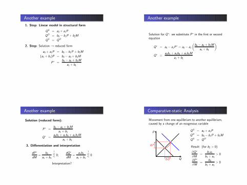
Another example
1. Step: Linear model in structural form
QS = a0 + a1P
QD = b0 − b1P + b2M
QS = QD
2. Step: Solution → reduced form
a0 + a1P = b0 − b1P + b2M
(a1 + b1)P = b0 − a0 + b2M
P∗ =b0 − a0 + b2M
a1 + b1
Another example
Solution for Q∗: we substitute P∗ in the first or secondequation
Q∗ = a0 − a1P∗ = a0 − a1
(
b0 − a0 + b2M
a1 + b1
)
Q∗ =a0b1 + a1b0 + a1b2M
a1 + b1
Another example
Solution (reduced form):
P∗ =b0 − a0 + b2M
a1 + b1
Q∗ =a0b1 + a1b0 + a1b2M
a1 + b1
3. Differentiation and interpretation
dP∗
dM=
b2a1 + b1
?
R 0;dQ∗
dM=
a1b2a1 + b1
?
R 0
Interpretation?
Comparative-static Analysis
Movement from one equilibrium to another equilibrium,caused by a change of an exogenous variable
P
Q∆Q
∆Pbc
bc
QS = a0 + a1P
QD = b0 − b1P + b2M
QS = QD
Result: (for b2 > 0)
∂Q∗
∂M=
b2a1b1 + a1
> 0
∂P∗
∂M=
b2b1 + a1
> 0

Comparative-static Analysis
Graphical Solution
Comparative-static Analysis
Graphical Solution:
3 Steps:
Decide whether the event shifts the supply ordemand curve (or both)
Decide whether the curve(s) shift(s) to the left orto the right
Examine how the shift affects equilibrium price P∗
and quantity Q∗
Comparative-static Analysis
Example:
If income increases consumer will be willing tospend more at any initial price (if it’s a normalgood), i.e., the demand curve shifts to the right
Suppliers have at the initial price no incentive tosupply more, they expand production only whenprice rises!
Therefore, a shift of the demand curve to theright causes an excess demand (shortage), thiscauses prices to rise, and suppliers adjust alongthe supply curve!
Dynamic of Adjustemnt
P
Q
bc bc
ExcessDemand
∆Q
∆P
bcAn exogeneous rise in in-come causes an excessdemand, . . .therefore price will in-crease and suppliers ad-just along the supplycurve.

Changes in Market Equilibrium
Qualitative forecast:Predicts only the direction in which an economicvariable will move
Quantitative forecast:Predicts both the direction and the magnitude of thechange in an economic variableEconometrics uses statistical tools (regressionanalysis) for making quantitative forecast
Examples
What is the effect of the following events onequilibrium quantity and price?
A strike in a firm on the goods market [⇓]
What is the effect of a decrease of average familysize on the market for 4-room apartments [⇓]
An increase in wages in a firm on the market ofthe good they produce [⇓]
Valentine’s day on the market for flowers [⇓]
A decrease in the price for Pepsi on the market forCoca-Cola [⇓]
A tax on electricity on the market for aluminium [⇓]
Skip Solutions
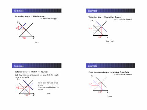
Example
Strike → Goods market: ⇒ decrease in supply.
P
Q∆Q
∆Pbc
bc
back
Example
Decreasing number of kids → market for largeapartments: ⇒ decrease in demand.
P
Q∆Q
∆Pbc
bc
back
Example
Increasing wages → Goods market:⇒ decrease in supply.
P
Q∆Q
∆Pbc
bc
back
Example
Valentin’s day → Market for flowers:⇒ increase in demand.
P
Q∆Q
∆Pbc
bc
fwd., back
Example
Valentin’s day → Market for flowers:
but: Expectations of suppliers can also shift the supplycurve to the right!
P
Q∆Q
∆P bcbc
Price can increase or de-crease,but quantity will always in-crease!
back
Example
Pepsi becomes cheaper → Market Coca-Cola:⇒ decrease in demand.
P
Q∆Q
∆Pbc
bc
back

Example
Tax on electricity → Market for aluminium:⇒ decrease in supply.
P
Q∆Q
∆Pbc
bc
back
Example: Price of Coffee
Why are coffee prices very volatile?Most of the world’s coffee is produced in BrazilMany changing weather conditions affect the crop ofcoffee, thereby affecting pricePrice following bad weather conditions is usuallyshort-livedIn long run, prices come back to original levels, all elseequal
Price of Coffee (1965 - 2003, nominal prices) Price of Coffee: short-run
P
Q
S1
Q1
D
P1
S2
P2
Q2
In the short run supply is(almost) perfectly inelastic(vertical)
A freeze decreases thesupply of coffee
Price increases significantlydue to inelastic supply anddemand.

Price of Coffee: long-run
P
Q
Slr
Qlr
D
Plr
In the long run supplyis extremely elastic(almost horizontal),demand is more elasticthan in the short run
Price falls back to Plr
Quantity falls back toQlr.
Shifts in Supply and Demand
When supply and demand change simultaneously,the impact on the equilibrium price and quantityis determined by:
The relative size and direction of the change.The shape of the supply and demand models.
Example: The Price of a Education
The real price of a college education in USA rose55 percent from 1970 to 2002.
Increases in costs of modern classrooms and wagesincreased costs of production – decrease in supply.Due to a larger percentage of high school graduatesattending college, demand increased.
Example: The Price of a Education
P
Q
S1970
D1970
P∗70
Q∗70
S2002
D2002
P∗02
Q∗02
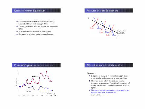
Resource Market Equilibrium
Consumption of copper has increased about ahundredfold from 1880 through 2002.
The long term real price for copper has somewhatfallen.
Increased demand as world economy grew.
Decreased production costs increased supply.
Resource Market Equilibrium
P
Q
D1900S1900
D1950S1950
D2005S2005
Long-Run Pathof Price andConsumption
Prices of Copper (1965 - 2002, real & nominal prices) Allocation function of the market
Summary:
Exogeneous changes in demand or supply causeprices to change in response to new scarcities.
This new prices affect demand and supplydecisions (prices act as ‘incentives’), behaviour ofmarket participants changes in response to pricesignals.
Therefore, competitive markets contribute to anefficient allocation of resources!(Details will follow . . . )

Value of Market Exchange:
Consumer- and Producer Surplus
Equilibrium & Welfare Economics
Market equilibrium reflects the way marketsallocate scarce resources
Whether the market allocation is desirable or notis determined by welfare positions of buyers andsellers
⇒ Welfare EconomicsBuyers and sellers receive benefits from taking part inthe market:→ Consumer surplus and producer surplusSum over consumer and producer surplus represents asociety’s total welfareEquilibrium in a market maximizes the total welfare ofbuyers and sellers
Consumer Surplus
Willingness to pay
Consumer will buy a good only if its benefit atleast covers its cost (price)
Willingness to pay: Maximum price that a buyeris willing and able to pay for a good
Reservation Price: Price at which a consumer isjust indifferent between buying and not buying →
Measures the willingness to pay.If you buy for the reservation price you are neitherbetter nor worse off, your cost equals your benefit!

Example
Willingness to Pay and Market Demand:
Willingness to payof A, B, C & D:
$A 20B 15C 10D 7
0
5
10
15
20
0 1 2 3 4
P
Q
7
bc
bc
bc
bc
bc
bc
bc
bc
bc
bc
bc
bc
Market Demand
Demand and willingness to pay
0
5
10
15
20
0 1 2 3 4
P
Q
7
bc
bc
bc
bc
Willingness to pay of A
Willingness to pay of B
WtP of C
WtP of D
Consumer Surplus
Consumer Surplus with P = 15:
0
5
10
15
20
0 1 2 3 4
P
Q
bc
bc
bc
bc
Total consumer surplus= consumer surplus of A= 1× 5 = 5A
Consumer Surplus
Consumer Surplus with P = 10:
0
5
10
15
20
0 1 2 3 4
P
Q
bc
bc
bc
bc
Total consumer Surplus= consumer surplus of A+ consumer surplus of B= 1× 10 + 1× 5 = 15
AB

Consumer Surplus
Consumer Surplus with P = 7:
0
5
10
15
20
0 1 2 3 4
P
Q
7
bc
bc
bc
bc
Total consumer Surplus= consumer surplus of A+ consumer surplus of B+ consumer surplus of C= 1× 13 + 1× 8 + 1× 3 = 24
AB
C
Consumer Surplus
Total consumer surplus and expenditures with P = 8:
0
5
10
15
20
0 1 2 3 4
P
Q
8
bc
bc
bc
bc
TotalConsumer Surplus
Total Consumer Surplus= 1× 12 + 1× 7 + 1× 2 = 21
Total Expenditures
Total Expenditures= 3× 8 = 24
Effects of a price cut
P
Q
QD
Initial consumer surplus
bc
bc
Additional consu-mer surplus toinitial consumers
bc
Consumer surplusto new consumers
(With many consumers the market demand curve is almost linear.)
Effects of a price cut
P
Q
QD
bc
Total additionalconsumer surplusof a price cut
bc

Consumer Surplus
Consumer surplus in the market is measured bythe area below the demand curve and above theequilibrium price
Consumer surplus is the amount that buyers arewilling to pay for a good minus the amount theyactually pay for it.
Consumer surplus measures the benefit thatbuyers receive from a good as the buyersthemselves perceive it
Consumer Surplus
Attention:
This concept of consumer surplus neglects tat achange in prices ceteris paribus also affects thepurchasing power!
Therefore it is only approximately valid
This concept of consumer surplus is only a limitedindicator for welfare, since it does not considerother aspects of welfare, like fairness or thedistribution of income
Producer Surplus
Producer Surplus
Producer will sell a product only when the price ofthe unit sold at least covers the cost of this unit
⇒ Marginal Cost: The cost of one additional unit(or the cost of the last produced unit respectively)

Example
Marginal Cost and Market Supply:
Marginal cost (MC)of 4 producersW, X, Y & Z:
MC ($)W 5X 12Y 17Z 22
Supply of W, X, Y & Zat different prices:
Price Seller(s) QS
P ≥ 22 W, X, Y & Z 417 ≤ P < 22 W, X & Y 312 ≤ P < 17 W & X 25 ≤ P < 12 W 1
P < 5 0
Example
Marginal Cost and Market Supply:
Marginal Cost ofW, X, Y & Z:
$W 5X 12Y 17Z 22
0
5
10
15
20
0 1 2 3 4
P
Q
bc
bc
bc
bcbc
bc
bc
bc
MC of W
MC of X
MC of Y
MC of Z
bc
bc
bc
bc
Supply Curve
Producer Surplus
At any quantity, the price given by the supplycurve shows the cost of the marginal seller, theseller who would leave the market first if the pricewere any lower
Just as consumer surplus is related to the demandcurve, producer surplus is closely related to thesupply curve
Producer Surplus: The area below the price andabove the supply curve measures the producersurplus in a market
Producer Surplus
Producer Surplus with P = 12:
0
5
10
15
20
0 1 2 3 4
P
Q
bc
bc
bc
bc
Total Producer Surplus= Producer Surplus of W= 1× (12− 5) = 7
W
12

Producer Surplus
Producer Surplus with P = 17:
0
5
10
15
20
0 1 2 3 4
P
Q
bc
bc
bc
bc
Total Producer Surplus= Producer Surplus of W+ Producer Surplus of X= 1× (17− 5) + 1× (17− 12)= 17
WX
17
Producer Surplus
Producer Surplus with P = 22:
0
5
10
15
20
0 1 2 3 4
P
Q
bc
bc
bc
bc
Total Producer Surplus= Producer Surplus of W+ Producer Surplus of X+ Producer Surplus of Y= 1× 17 + 1× 10 + 1× 5 = 32
WX
Y
22
Effects of a price increase
P
Q
QS
Initial producer surplus
bc
bc
additional pro-ducer surplusto initialproducers
producersurplus tonew producers
Effects of a price increase
P
Q
QS
Total additionalproducer surplus
bc
bc

Equilibrium & Welfare
Demand and Supply Function
0
5
10
15
20
0 1 2 3 4
P
Q
bc
bc
bc
bc
MC W: 5
MC X: 12
MC Y: 17
MC Z: 22bc
bc
bc
bc
WtP A: 20
WtP B: 15
WtP C: 10WtP D: 7
MC: Marginal Cost WtP: Willingness to Pay
Equilibrium & Welfare
Free markets allocate the supply of goods to thebuyers who value them most highly
Free markets allocate the demand for goods tothe sellers who can produce them at least cost
Free markets produce the quantity of goods thatmaximizes the sum of consumer and producersurplus
Equilibrium & Welfare
P
Q
QS
QD
bcValueto
buyersCost toproducers
Value to buyersis greater thancost to sellers!
Cost toproducers
Value tobuyers
Value to buyersis less than
cost to sellers!

Equilibrium & Welfare
Consumer-surplus
=Value toconsumers
−Amount paidby consumers
Producer-surplus
=Revenue ofproducers
−Cost toSellers
TotalSurplus
=Value to
Consumers−
Cost toSellers
Equilibrium & Welfare
P
Q
QS
QD
Consu-mer surplus
Producersurplus
bc
Market efficiency is achieved whenthe allocation of resources
maximizes totalsurplus!
P∗
Q∗
Market Efficiency
Market outcome is often not efficient
⇒ Market failure: Examples includeMarket powerExternalitiesPublic goodsAsymmetric informationPrice regulation . . .
Apart from efficiency, a social planner might alsocare about equity: Fairness of the distribution ofwell-being among the various buyers and sellers
Welfare Effects of PriceRegulations

Welfare effects of price floors
Effects of a price floor: Pmin = 7
0
2
4
6
8
10
0 2 4 6 8 10 12 14 16 18
P
Q
7Pmin = 7
bc
Consumer surplus
Producer surplus
Dead-weightloss
Welfare effects of price ceilings
Effects of a price ceiling: Pmax = 4
0
2
4
6
8
10
0 2 4 6 8 10 12 14 16 18
P
Q
bc Pmax = 4
Producer Surplus
Consumer-surplus
Dead-weightloss
Price Regulation and Deadweight Loss
Notice: The total amount of the deadweight lossdepends on ...
how distant the price floor/ceiling is away fromthe equilibrium price, and
the slopes of demand and supply curves
An Application:
International Trade

International Trade
If a country is isolated from rest of the world(under autarky) domestic price adjusts to balancedemand and supply.
The sum of consumer and producer surplusmeasures the total benefits that buyers and sellersreceive.Can international trade further improve thissituation?
International Trade
If a country has a comparative advantage, thenthe domestic price will be below the world price,and the country will be an exporter of the good.
If the country has a comparative disadvantage,then the domestic price will be higher than theworld price, and the country will be an importer ofthe good.
Two Countries before International Trade
Consumer and producer surplus under autarky:
Country 1 Country 2P
Q
P
QCountry 2 has a comparative advantage in the production of thisgood, i.e., it can produce the good cheaper!
International Trade
Consumer and producer surplus with trade:
Country 1 (Importer) Country 2 (Exporter)P
Q
PW
Imports
bc bc
QS QD
P
Q
Exports
bc bc bc bc
QSQD

International Trade
Consumer and producer surplus with trade:
Country 1 (Importer) Country 2 (Exporter)P
Q
PW
Imports
Net-gain of
consumersurplus
bc bc
QS QD
P
Q
Exports
Net-gain ofproducersurplus
bc bc bc bc
QSQD
International Trade and Welfare
Consequences for importing countries:Domestic producers of the good are worse off, anddomestic consumers of the good are better off.If welfare of producers and consumers is equallyweighted trade raises the economic well-being of thenation as a whole.
Consequences for exporting countries:Domestic producers of the good are better off, anddomestic consumers of the good are worse off.Again, trade raises the economic well-being of thenation as a whole.
Trade Policy
Tariffs
Tariffs are taxes on imported goods.
Tariffs raise the price of imported goods above theworld price by the amount of the tariff.
A tariff reduces the quantity of imports and movesthe domestic market closer to its equilibriumwithout trade.
With a tariff, total surplus in the market decreasesby an amount referred to as a deadweight loss.
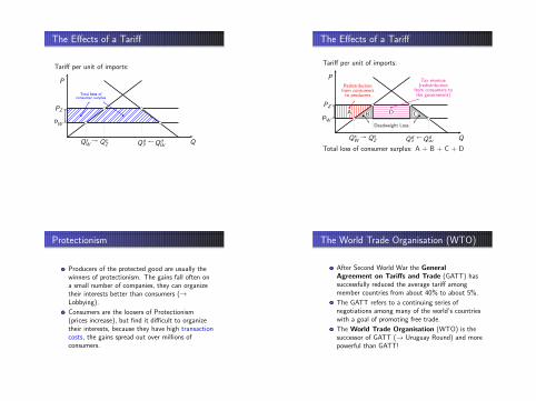
The Effects of a Tariff
Tariff per unit of imports:
P
Q
PW
QsW Qd
W
bc bc
PZ
QsZ Qd
Z
bc bc
bc bc
bc bc
Total loss ofconsumer surplus
The Effects of a Tariff
Tariff per unit of imports:
P
Q
PW
QsW Qd
W
bc bc
PZ
QsZ Qd
Z
bc bc
A
Redistributionfrom consumersto producers
D
Tax revenue(redistribution
from consumers tothe government)
B C
Deadweight Loss
bc bc
bc bc
Total loss of consumer surplus: A + B + C + D
Protectionism
Producers of the protected good are usually thewinners of protectionism. The gains fall often ona small number of companies, they can organizetheir interests better than consumers (→Lobbying).
Consumers are the loosers of Protectionism(prices increase), but find it difficult to organizetheir interests, because they have high transactioncosts, the gains spread out over millions ofconsumers.
The World Trade Organisation (WTO)
After Second World War the GeneralAgreement on Tariffs and Trade (GATT) hassuccessfully reduced the average tariff amongmember countries from about 40% to about 5%.
The GATT refers to a continuing series ofnegotiations among many of the world’s countrieswith a goal of promoting free trade.
The World Trade Organisation (WTO) is thesuccessor of GATT (→ Uruguay Round) and morepowerful than GATT!

The World Trade Organisation (WTO)
WTO Rules:
Non-discrimination: Under the ‘most favorednations clause’, any trade concession that onecountry makes one member must be granted to allsignatories.
Reciprocity: Any nation benefiting from a tariffreduction by another country must reciprocate bymaking similar tariff reductions itself.
Furthermore: General prohibition of quotas, Faircompetition, Binding tariffs.
Any questions?
Thanks!