Portland State University Portland State University

PDXScholar PDXScholar

Dissertations and Theses Dissertations and Theses

7-22-1994

Building of a Thermoacoustic Refrigerator and Building of a Thermoacoustic Refrigerator and

Measuring the Basic Performance Measuring the Basic Performance

Torsten Blumreiter Portland State University

Follow this and additional works at: https://pdxscholar.library.pdx.edu/open_access_etds

Part of the Physics Commons

Let us know how access to this document benefits you.

Recommended Citation Recommended Citation Blumreiter, Torsten, "Building of a Thermoacoustic Refrigerator and Measuring the Basic Performance" (1994). Dissertations and Theses. Paper 4714. https://doi.org/10.15760/etd.6598

This Thesis is brought to you for free and open access. It has been accepted for inclusion in Dissertations and Theses by an authorized administrator of PDXScholar. Please contact us if we can make this document more accessible: pdxscholar@pdx.edu.

THESIS APPROVAL

The abstract and thesis of Torsten Blumreiter for the Master of Science in Physics were

presented July 22, 1994, and accepted by the thesis committee and the department.

COMMITTEE APPROVALS:

DEPARTMENT APPROVAL:

Laird C. Brodie "l

Paul Latiolais / .. Representative of the Office of Graduate Studies

Enk'·Bcxlegom, Chair Department of Physics

* * * * * * * * * * * * * * * * * * * * * * * * * * * * * * * * * * * * * * * * * * * * * *

ACCEPTED FOR PORTLAND STATE UNIVERSITY BY THE LIBRARY

by~ ·If

Oni<l;,~ £i4·em4-lf· /<??1

ABSTRACT

An abstract of the thesis ofTorsten Blumreiter for the Master of Science in Physics

presented July 22, 1994

Title: Building of a thennoacoustic refrigerator and measuring the basic performance

The application of thennoacoustic phenomena for cooling purposes has a comparatively

short history. However, recent experiments have shown that thennoacoustic refrigeration

can achieve practical significance for both every day cooling in households and

cryocooling for scientific purposes due to its high reliability, environmental safety and

functioning under extreme conditions.

We build a thermoacoustic refrigerator driven by a commercial loudspeaker. It was

equipped with a vacuum pump and an entrance port for introducing different gases under

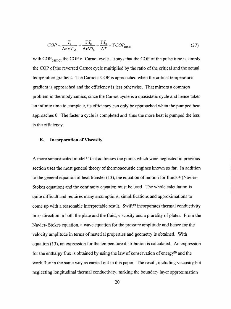
different pressures as working fluids. It contained two thermocouples and a pressure

transducer for quantitative measurements of the basic perfonnance.

The resonance frequency of the tube for different gases has been determined and

compared to the theoretical value. The temperatures of the hot and the cold heat

exchanger have been measured.

Also, a simple thennoacoustic oscillator for demonstration purposes was built. After

immersing one end in liquid nitrogen or heating up the other end with a bunsen burner it

started to oscillate and emit a sound.

BUILDING OF A THERMOACOUSTIC REFRIGERATOR AND MEASURING

THE BASIC PERFORMANCE

by

TORSTEN BLUMREITER

A thesis submitted in partial fulfillment of the requirements for the degree of

MASTER OF SCIENCE m

PHYSICS

Portland State University 1994

Table of Contents

Table of Contents ......................................................................................................... ii

L . f . . 1st o Figures .............................................................................................................. 1v

List of Tables ................................................................................................................ v

Acknowledgements ..................................................................................................... vi

CHAPTER 1: Introduction ........................................................................................... 2

CHAPTER 2: Theory of Thermoacoustic Engines ...................................................... .4

2.1 Qualitative Description of a Thermoacoustic Refrigerator ......................... 4

2.2 Theoretical Treatment ................................................................................. 4

A. Introduction .................................................................................... 2

B. Properties of Sound Waves ............................................................ 9

C. Oscillatory Temperature ............................................................... 12

D. Heat Flux, Work Flux and Efficiency .......................................... 16

E. Incorporation ofViscosity ............................................................ 20

2.3 Summary of Working Conditions and Working Fluids ............................ 22

2 .4 Resonator Geometry ................................................................................. 26

CHAPTER 3: Experimental Setup and Construction ................................................. 28

A. The Driver ................................................................................................ 29

B. The Heat Exchangers ............................................................................... 30

C. The Stack .................................................................................................. 31

D. The Resonator .......................................................................................... 32

E. Vacuum and Helium ................................................................................. 33

F. Instrumentation and Measurements .......................................................... 34

G. Demonstration Tube ................................................................................ 36

CHAPTER 4: Experimental Results and Conclusions .................................................... 38

4.1 Results ............................................................................................................ 38

4.2 Conclusions .................................................................................................... 40

List of Figures

Figure 1: Sketch of the work principle of a prime mover and a heat pump .................... .4

Figure 2: Drawing of the pulse tube used in this experiment (units in inch) ................... 5

Figure 3: Four- step- cycle of a fluid parcel near a plate ................................................. 7

Figure 4: p-V-diagram of a complete cycle ..................................................................... 8

Figure 5: The thermoacoustic cycle in a s-T-diagram ...................................................... 9

Figure 6: Schematic of four possible resonator geometries ............................................. 26

Figure 7: Picture of the modified speaker with the aluminum cone replaced the

soft dome .......................................................................................................................... 30

Figure 8:'String alignment jig and section of the plastic film ........................................... 31

Figure 9: Picture of the rolled up stack ............................................................................ 32

Figure 10: Drawing of the vacuum and helium filling system ......................................... 34

Figure 11: Calibration curve of the thermocouple in conjunction with an amplifier,

with one junction in an ice bath and the other junction in water ..................................... 35

Figure 12: Drawing of a simple thermoacoustic oscillator .............................................. 36

Figure 13: Voltage signal of the pressure tranducer in arbitrary units as a function

of the frequency for air (p= 1 atm, T=20 C) ..................................................................... 39

Figure 14: Voltage signal of the pressure transducer in arbitrary units versus the

frequency for helium (p=l atm, T=20 C) ......................................................................... 39

List of Tables

Table 1: Some thermodynamic properties related to the performance of a

thermoacoustic engine of various gases at their resonance frequency in the

resonator used in this experiment at the same temperature and pressure (p= 1 atm,

T=273K) ........................................................................................................................... 23

Table 2: Prandtl number and viscous diffusity for various gases for T=273K ................ 25

Table 3: Calculated and experimentally determined resonance frequency for

T=20C .............................................................................................................................. 38

Acknowledgements

I am very thankful to Mr. Rudolf Zupan from the science support shop for his continuous

and fine work.

I would like to thank Dr. Erik Bodegom, my academic adviser, for his many useful

suggestions.

I would like to acknowledge the flexibility of the committee members Laird C. Brodie,

Paul Latiolais and Erik Bodegom.

CHAPTER 1: Introduction

Thermoacoustics is a branch of physics dealing, as the word already reveals, with

thermodynamics and acoustics. Specifically, it relates to the transfer of heat, work,

enthalpy, and other thermodynamic quantities and to the conversion of heat energy into

other kinds of energy and vice versa by using acoustic phenomena or sound waves1•

In this research, thermoacoustics is applied to a refrigerating system in which sound

waves are used for transferring heat from a location of lower temperature to one of higher

temperature (heat pump). The usage of sound waves has some significant advantages

compared to current refrigerating systems. The only moving part is the sound generating

part, a voice coil of a regular commercial loudspeaker. This coil can be driven quite

inexpensively by a simple amplifier. This amplifier needs only to amplify one sinusoidal

frequency, the resonance frequency of the refrigerator. Good acoustic insulation can

make the refrigerator fairly quiet. It is also an environmentally significant step to safe

technology, because no chlorofluorocarbons (CFCs) are released.

The history of thermoacoustics goes back to the glassblowers in the 18th and 19th

century. Sometimes, while blowing their glass tubes, a loud sound occurred. First

experiments were probably done by Byron Higgins in 1777, who was able to excite organ

pipe oscillations in a large tube, open at both ends, by suitable placement of a hydrogen

flame inside. The best known thermoacoustical devices in history are the Sondhauss tube

and the Rijke tube, introduced in 1850 and 1859, respectively. The Soundhauss tube was

an open tube of about 15 cm made of glass with a sphere on top. After heating the closed

end or spherical end it started to produce and maintain a vibration.

Probably, the best known example of the excitation of sound waves is known as "Taconis

oscillations" that occur when a tube, closed on the top, is inserted in a liquid helium

dewar. They were systematically observed by Clement and Gaffney and recently some

2

quantitative experiments were done by Yasaki2.

The history of serious and systematic research of the reverse process is quite short. The

first experiments were done by Gifford and Longsworth2. They operated the Sondhauss

tube in reverse, i.e. they produced a temperature difference by applying a low- frequency,

high- amplitude acoustic wave to the gas in a tube. They called their device a pulse tube.

Later experiments were done by a group of researchers in Los Alamos, California in the

eighties. Their experiments resulted in an almost practical refrigerator, and theory and

experimental results3 were compared.

The Russian scientist E.I. Mikulin4 used a different technique. He outfitted the original

pulse tube with an orifice. This orifice allows the gas to expand through the orifice into a

large reservoir. This increased the refrigeration capacity considerably.

According to Rott1, the creation of the field of theoretical thermoacoustics goes back to

Kirchhoff in 1868. In 1896, Lord Rayleigh discussed, although more qualitatively in

nature, the phase difference between temperature and motion. The most complete

quantitative theory was introduced and developed by Rott and co- workers in the sixties

and seventies.

3

CHAPTER 2: Theory of Thermoacoustic Engines

2.1 Qualitative Description of a Thermoacoustic Refrigerator

When talking about conversion of heat into work, two concepts always appear: prime

mover and heat pump (see figure 1 for a schematic representation of both engines

indicating the flow of energy). A prime mover requires a cold and hot heat exchanger and

by transferring heat from the hot to the cold exchanger, work can be done. (That was the

way the glass blowers generated their sounds and the way the Sondhauss tube worked.)

The reverse device called heat pump transfers heat from the cold to the hot heat

exchanger by absorbing work. Both machines typically work in cycles and in a steady

state which means that the state of the heat exchangers after one cycle has not changed.

Prime mover Heat pump

hot hot i I //·~~

Q H

i I

~/ I I Q H

'W I

W I

Engine ~ ~1 L/ Engine ! ~-1

[

QC ~; /> LJ Q c

cold cold

Figure I: Sketch of the work principle of a prime mover and a heat pump

The acoustic refrigerator (pulse tube) is a heat pump that absorbs acoustic power

4

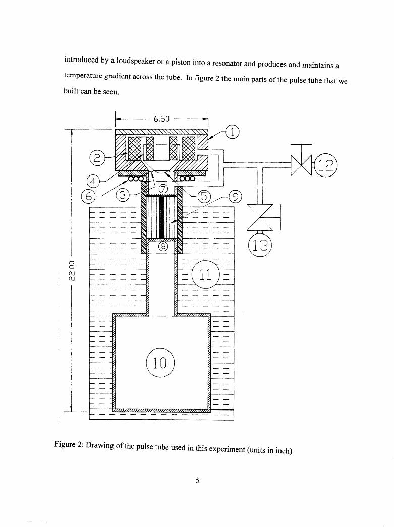
introduced by a loudspeaker or a piston into a resonator and produces and maintains a

temperature gradient across the tube. In figure 2 the main parts of the pulse tube that we

built can be seen.

r 1--

0 a (\J (\J

@___,/~~

®~

6.50

@

-1

~ ~~®

,/

Figure 2: Drawing of the pulse tube used in this experiment (units in inch)

5

The labeling numbers mean the following:

1 . -speaker housing

2. -magnet

3. -extra surround

4. -voice coil

5. -aluminum cone

6. -cooling tubes

7. -hot heat exchanger

8. -cold heat exchanger

9. -stack

10. -cold section

11. -insulation

12. -vacuum pump valve

13. -helium regulator valve

The essential parts are the speaker on top (2 and 4), the stack of poor heat conducting

plates (9) between two heat exchangers (7 and 8) and the resonator. The speaker

maintains a standing acoustic wave in the resonator. The principle of thermoacoustic

refrigerators can be understood by considering small fluid parcels moving back and forth

between a state of compression and expansion. In an undisturbed standing wave no heat

transfer and work absorption would occur, except for dissipative losses. This is changed,

however, in the presence of a second medium. To illustrate, a complete cycle that a fluid

parcel goes through near a plate, is shown in four steps in figure 3.

6

~ v ~

2

a) b)

[J I I dW 1 l__j -----> I

c) 2 d)

~ n

Figure 3: Four- step- cycle of a fluid parcel near a plate

2

• I

IC I dQ

2

I __ J dQ

Step a) shows the adiabatic compression of the parcel due to increased pressure resulting

in the associated movement to the right, a decrease in volume and increase in

temperature. At the farthest point on the right hand side, heat transfer from the heated

parcel to the plate takes place. This results in a volume and temperature decrease of the

parcel. Step c) describes the adiabatic expansion due to decreased pressure. As the

parcel moves to the left it cools down further and expands. Lastly, step d) completes the

cycle. Since the temperature has decreased below the plate's temperature, heat is being

transferred from the plate to the parcel. It is accompanied by an increase in volume and

temperature. Considering a complete cycle, heat is being transferred from the left to the

right hand side as well as work being done in the expanded state and absorbed in the

7

compressed state. Since the temperature in the compressed state is higher, net work has

been absorbed. In figure 4, the cycle is shown in a p-V- diagram.

p

l -----

Figure 4: p-V-diagram of a complete cycle

The heat flow is equivalent to an entropy flow. Steps a) and c) are nearly adiabatic,

therefore the entropy of the parcel remains constant. In position 1 in figure 3d, heat is

being picked up from the plate which results in an entropy increase of ~s. This amount is

carried from the position 1 to position 2 where it is returned to the plate. Hence, in half a

cycle entropy of ~s has moved from the left to the right.

8

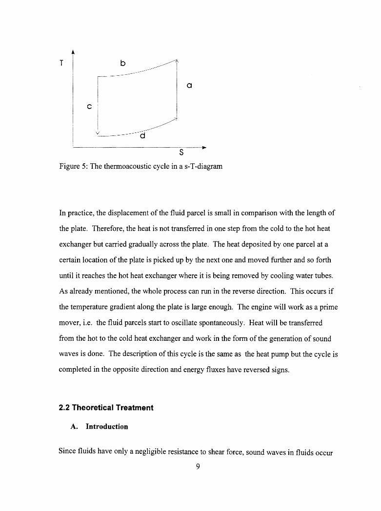
t T I

I

b /!'\

I

I I C I I

L_~-cj/

a

s Figure 5: The thermoacoustic cycle in a s-T-diagram

In practice, the displacement of the fluid parcel is small in comparison with the length of

the plate. Therefore, the heat is not transferred in one step from the cold to the hot heat

exchanger but carried gradually across the plate. The heat deposited by one parcel at a

certain location of the plate is picked up by the next one and moved further and so forth

until it reaches the hot heat exchanger where it is being removed by cooling water tubes.

As already mentioned, the whole process can run in the reverse direction. This occurs if

the temperature gradient along the plate is large enough. The engine will work as a prime

mover, i.e. the fluid parcels start to oscillate spontaneously. Heat will be transferred

from the hot to the cold heat exchanger and work in the form of the generation of sound

waves is done. The description of this cycle is the same as the heat pump but the cycle is

completed in the opposite direction and energy fluxes have reversed signs.

2.2 Theoretical Treatment

A. Introduction

Since fluids have only a negligible resistance to shear force, sound waves in fluids occur

9

only longitudinally, i.e., the direction of propagation is the same as the movement of the

molecules carrying the wave. The molecules move irregularly and randomly. In the

presence of a sound wave an averaged directed motion in the direction of the wave

propagation takes place. This causes a change in pressure and hence a backdirected force

towards the original state. The usual treatment of sound waves is macroscopic. This

means that individual molecular motions are neglected and only a macroscopic fluid

parcel, yet small enough to be treated as an infinitesimal, is considered.

As long as the displacement of the molecules is proportional to the backdirected force, we

speak of harmonic waves. This leads to a linear differential equation describing the

behavior of the wave. If the areas of equal phase and amplitude are planes, perpendicular

to the direction of propagation, the wave is said to be plane.

In acoustics, the pressure and the oscillatory velocity of the fluid parcel are often used to

describe the sound wave. We assume that the amplitude of the sound wave is small

compared to the average pressure. We will assume that all oscillating quantities (such as

temperature, entropy) are small and non- linear terms can be ignored. Or, in

mathematical terms, every quantity is expanded in a power series and second and all

higher order terms are neglected. These variation terms are designated by a subscript 1

while the equilibrium quantities are designated by subscript 0.

The complex notation for physical quantities is consequently used for the calculations,

although the physics is described just by the real part.

B. Properties of Sound Waves

The one dimensional wave equation for the pressure p1 is5:

a2P1 - I a2P1 ax2 --;r at2

10

(1)

with c = 1(i) defined as the phase velocity of the sound wave. The most simple p p=po

solution is described by the trigonometric functions using the customary complex Euler-

notation and convenient boundary conditions:

P1 = p Aei(kx-cor)

whereas ro is angular frequency of the wave. From Euler's equation for fluids6,

describing a relationship between the pressure of the sound wave and the oscillatory

velocity v1 of a parcel, and the well known relation of the phase velocity

c=Af=ro k

the following expression for v1 is obtained:

v1

= _!_ J ~t = PA ei(kx-cor)

Po Bx PoC

(2)

(2a)

(3)

In our experiments we deal exclusively with standing waves. In a pipe, standing wave

patterns are built up due to superposition of the initial and the reflected wave. Thus, the

pressure at a certain point can be calculate~ just by adding up the pressures of the back

and forth traveling wave, or:

P1 = p: + p1- = PA(ei(k.x-cor) +ei(-k.x-cor)) (4)

This can be simplified to:

P1=2pA coskx e·icor (5)

The oscillatory velocity in the standing wave is obtained by substituting ( 5) in (3) as

follows:

11

v = i 2 p A sin kx e-irot I

PoC (6)

Considering only the real part of either formula, it can be seen that the spatial and the

temporal part of a standing wave are not coupled anymore. Also, unlike the traveling

wave, there is a constant phase shift of Tt/2 between the pressure and velocity for both the

temporary and the spatial part as indicated by the imaginary unit and the different

trigonometric functions. It follows that the pressure antinode is at a location where the

velocity node is and vice versa.

C. Oscillatory Temperature

The next step is to derive a relationship between the pressure and the temperature

distribution in the bulk gas for a standing wave. The temperature is considered to consist

of a mean temperature T0 and a small variation in the x-direction T1 (the linear term of

the power series expansion) and to be constant in y- direction. With the assumption of

small pressure and temperature variations, assuming an adiabatic process, T 1 can be

written as

I;= (8TJ 8p P1 s

(8)

By using the well-known Maxwell relation? we obtain:

r. = __ 1 (ap) I 2 -p as P1

0 s

(9)

which can be reworked to:

1 (ap) (ar) Ta~ :z; = - p: OT ' Os P Pi = Poe' Pi

(10)

12

with c P = _!_ ( oH) = To ( os ) the isobaric heat capacity8, m8TP m8TP

1 (av) 1 (op) and p = V 8T P = - Po 8T P

the thermal expansion coefficient at constant pressure9.

(lOa)

(lOb)

All those relationships are derived by expanding the partial derivatives and by applying

the general chain rule and using the Maxwell relations.

For an ideal gas, we obtain:

( 8T) _ ToP _ y -1 Ta - -----Op s PoCp Y Po

( 11)

by using the adiabatic equation for an ideal gas

1-y

Tp r = constant. (12)

So far, we only considered the waves in the bulk phase of the gas.

By introducing a plate as a second medium, those simple relations change considerably.

So far, we have no y- dependence of the temperature, no heat transfer takes place and

pressure and temperature are in phase. The second medium causes a thermal lag between

temperature and motion in the fluid. To calculate the temperature distribution in the

presence of a plate, simplifications must be made.

1) Viscosity is neglected. This assumption is not realistic but simplifies the

calculation considerably. For that reason it is going to be added to the final result

by means of an estimate.

2) The amplitudes of pressure and velocity are assumed to be constant all over the

plate since the plate is short enough with respect to the wavelength.

3) Heat transfer due to thermal conduction occurs only in y- direction and is neglected

13

in the x direction (see the definitions of the directions in figure 3) both through the

plate and the fluid. This approximation can be made in the fluid since the heat flux

due to convective heat flow is much larger and faster, and in the plate since the

material of the plate is chosen to be poor with respect to thermal conduction.

4) All mean physical quantities, e.g. T0, p0 ,s0 ••• are constant in space and time.

5) Beside the mean physical quantities and the first order terms, all higher order terms

are neglected.

6) From now on, the exponential time factor eiror that all oscillating quantities have in

common will be suppressed. i vI will be replaced by vI for convenience.

One starts with the general equation of heat transfer10:

Tp(:; +v• Vs)= V •(KV'T) (13)

where s is the entropy per unit mass and K the thermal conductivity.

This equation describes the change of entropy at a given point due to convective flow of

entropy and thermal conduction of heat. Quadratic terms of the velocity describing

entropy changes due to viscosity are neglected according to the assumptions mentioned

before. The entropy is considered to consist of a constant part so plus a small variation s1

according to the introduced notation. This assumption as well as the existence of only an

x- component of the velocity and the neglect of thermal conduction in x- direction

simplifies equation (13) as follows:

(as as) a2

T Pol'o at + v1 8x = K ay2 (14)

To eliminate the derivatives of s, the generalized chain rule for the two- dimensional case

is used:

14

: = ( :~ Lnst;Tof, °: + (:) T•<onst;n0

:

(15)

and a similar expression for the time derivative. With equation (lOa) and (lOb) and one

of the Maxwell equationsII we obtain:

(as) cp

BT p=const;T=To = To and (16)

(: Lon•t;p•p., = P:2 (;~ Lon'1;p•p, = - :. (17)

Substituting (15), (16), (17) into (14), a differential equation for the temperature TI is

obtained.

. T. K a2 r; . TA aro 1rop0cP 1 - --2 = 1ro10pp1 -p0cP -v1 ay ax (18)

The solution for this equation with boundary conditions that T 1 near the plate assumes the

temperature of the plate and far away from the plate is still finite, isI2:

1 P1 ---v1 l-e 0k

T. = ( To~ 1 BT )( _<i+i)y) PoCp (J) ax

(19)

with I> k = ) 2

K the thermal penetration depth, the characteristic length for thermal ropoc P

diffusion between a gas and a solid boundary. Equation (19) describes the temperature

behavior of the fluid at a certain location x with respect to the plate's temperature.

If the fluid is far enough away from the plate, y >> 8k, the exponential term can be

neglected and equation (19) becomes

15

T. = ( I'oP 1 BT ) I,yocok P1 ---Vi .

PoC p (t) ax (20)

The first term is identical with equation (10) and the second term is due to the

temperature gradient in x- direction throughout the fluid. If the temperature gradient

approaches a critical value, the second term will completely compensate the first term, i.e.

fluid and plate have the same temperature at every location. This turns out to be the

boundary between working as a refrigerator and a prime mover.

( BT) = T.~w:, = VJ;n, ax crit Po p I

(21)

As well as for the other quantities, the actual temperature distribution is described by the

real part of formula ( 19). The imaginary part, however, has significance for the work and

heat flux and is therefore shown explicitly in the next equation:

lm(J;) = - 0,..,-p1 ---v1 e 0k sin-

( Tr A 1 BT ) _1'._ y

PoC p (t) ax (\ (2la)

D. Heat Flux, Work Flux and Efficiency

As is customary in hydrodynamics, the convective flow of a physical quantity can be

found out by considering a large volume of fluid and a small cylinder of the fluid carrying

a certain amount of that quantity and entering the large volume through a surface element

dA with a velocity v1. Then, in a time ..M, the length v..1t of the cylinder will have crossed

the surface. Hence, the total heat load entering the volume is

..1Q = J Mp0Tov1s1dA (22)

by using the relationI3

dq = T(Xls = ~p0s1 (23)

16

with s the entropy per unit mass and q the heat per unit volume. The heat flux in steady

state is obtained by dividing equation (23) by .1t and time averaging. The surface element

in this particular case is the width of the plate TI times dy.

Q = TI J I'oPo ( S1 V1 )dy (24)

The integrand in formula (24) is the heat flux density q .

iJ =~Po (s1v1) (24a)

s 1 can be expressed in terms of T 1 and p 1 by using the formula for the total differential

and equation (16) and (17). For the time averaged product the well-known relation14

(AB)= tRe(AB*) (25)

with the asterix designating the complex conjugate can be used. After performing the

previous explained steps and considering that (p1v1 ) = 0, for the heat flux density in x-

direction is obtained:

q = t Pc,C P Im( J;)v1 (26)

After applying equation (24) to carry out the integral, the total heat flux15 is obtained to

be

• Q = tTII'o8kPP1V1 (r-1) (26a)

where r is the ratio between the temperature gradient and the critical temperature

gradient.

This formula reveals the following, partly expected results:

The heat flux is proportional to the area TI8 k • It is also proportional to the product of the

pressure and the oscillating velocity amplitudes. Since those are 74' 'A apart the maximum

17

heat transfer occurs right in the middle of the pressure and velocity antinodes. Lastly, the

heat flux decreases as the temperature gradient approaches the critical temperature

gradient. The heat flux density is greatest with respect to they-direction when the

imaginary part of T 1 is greatest. This occurs about a penetration depth away from the

plate (cf. equation (21a)).

To calculate the absorbed net work rate, the work per unit volume done by a differential

volume as it expands from V to V +dV is to be considered.

dV = P dp dw=-p v p

Divided by the total time differential it yields:

dw pdp -=--dt p dt

For pin the power series expansion the first approximation (p =Po+ p 1ei00') can be

substituted and the total time derivative of p in equation (28) can be expanded.

apo dp = ap +(v•V')p=icop, +v, ax dt at

(27)

(28)

(29)

After performing the two latter steps, four terms occur in (28). Three of the four terms

vanish after time averaging since (p1) = ( v1) = (p1 v1) = 0. The following remains

w = !!!__(iP1P1) Po

(30)

as the average acoustic power produced per unit volume. p1 can be expanded in terms

of T 1 and p 1 by using the formula for the total differential and after computing the

various derivatives, the following formula for the acoustic power absorbed per unit

volume is obtained:

18

w = -rop(ip11'i) = troPp1 Im(I'i) (31)

This formula shows, similar to the heat flux, that the work done or absorbed is greatest a

penetration depth away from the plate (see formula (21a)). It can be integrated over the

whole space to obtain the total time averaged acoustic power absorptionI6:

Clj

W = J wdV =-II& J ¥oPP1 lm(I'i)dy (32) (V) 0

w - J_ II8 Llx ToP2

ro 2 er -1) - 4 k P1 (33)

PoCp

whereby Llx is the length of the plate. As can be seen the total acoustic power absorbed is

proportional to the volume generated by the plate surface and the penetration depth, to the

square of the pressure amplitude and to the temperature gradient factor ( r - 1) that

already appeared in the heat flux.

The thermal efficiency of a prime mover is defined as the ratio of the work done and the

heat load of the hot heat exchanger.

w w 11=-=-

QH QH (34)

For a heat pump, an equivalent so-called COP (coefficient of performance) is defined just

as the reciprocal value.

COP= QH - QH w-w By dividing equation (26) and (33) the COP for this application can be obtained.

V1P0Cp

COP = &prop1

With formula (21) and the definition for the r it can be written

19

(35)

(36)

COP= To = 11'o 11'o ll:xVT = - = rcoP crit flx Y' fa f!i T carnot

(37)

with COP carnot the COP of Carnot cycle. It says that the COP of the pulse tube is simply

the COP of the reversed Carnot cycle multiplied by the ratio of the critical and the actual

temperature gradient. The Carnot's COP is approached when the critical temperature

gradient is approached and the efficiency is less otherwise. That mirrors a common

problem in thermodynamics, since the Carnot cycle is a quasistatic cycle and hence takes

an infinite time to complete, its efficiency can only be approached when the pumped heat

approaches 0. The faster a cycle is completed and thus the more heat is pumped the less

is the efficiency.

E. Incorporation of Viscosity

A more sophisticated model 17 that addresses the points which were neglected in previous

section uses the most general theory of thermoacoustic engines known so far. In addition

to the general equation of heat transfer (13), the equation of motion for fluids 18 (Navier­

Stokes equation) and the continuity equation must be used. The whole calculation is

quite difficult and requires many assumptions, simplifications and approximations to

come up with a reasonable interpretable result. Swift19 incorporates thermal conductivity

in x- direction in both the plate and the fluid, viscosity and a plurality of plates. From the

N avier- Stokes equation, a wave equation for the pressure amplitude and hence for the

velocity amplitude in terms of material properties and geometry is obtained. With

equation ( 13 ), an expression for the temperature distribution is calculated. An expression

for the enthalpy flux is obtained by using the law of conservation of energy20 and the

work flux in the same way as carried out in this paper. The result, including viscosity but

neglecting longitudinal thermal conductivity, making the boundary layer approximation

20

(y0 >> 8 k) and assuming a short plate is shown in the next two formulas21:

i-I = _ _!_ 8 n J:PP1 (vi) (r - 1)-n( K) d~ 4 k 1-~ Yo dx

(38)

W = _!_ mi,Ax ( y-l)~p12 (r -1)-_!_ Ill\Axcop0(vi)2

4 p0a 4 (39)

where (v1) is the averaged velocity over they-direction. (In that model, the velocity has

gotten an additional y- component22.)

iI is the enthalpy flux (includes both heat and work flux), cr the Prandtl number defined

as

cr=c:=(U withµ the viscosity, K the thermal conductivity and Cp the isobaric heat coefficient.

o" =) 2µ co po

(40)

(41)

is the fluid's viscous penetration depth. It can be interpreted as a characteristic length of

interaction between gas and a solid boundary for momentum diffusion. Yo is the plate's

spacing. The Prandtl number is a dimensionless quantity describing the amount of

momentum diffusion relative to thermal diffusion or in other words viscosity to thermal

conductivity.

Some additional results for practical usage can be extracted from the two latter equations.

The second term in the equation (39) is the power dissipated by viscous shear in the fluid

of the boundary layer. Therefore, gases with low viscosity and hence a low Prandtl

number work best. Due to dissipative losses, the idea of a critical temperature gradient

has to be replaced by a critical temperature range bordered by either one of the conditions

21

W = 0 and Q = 0. In that range, only losses occur and heat is transferred from the hot to

the cold heat exchanger while the net work is negative.

2.3 Summary of Working Conditions and Working Fluids

The theoretical treatment yields some qualitative statements concerning geometry, the

choice of the working fluid and thermodynamic conditions for the best possible

performance of the refrigerator. Ff\.'."} ~'

'j,,:1· \j

It is desirable to have a large heat transfer because the critical temperature gradient is

approached faster and a larger volume can be cooled. The work absorbed should also be

large. In equation (26a) and (33), and (38) and (39), respectively, it can be seen how the

working conditions and the properties of the working fluid affect the performance of the

refrigerator. All these equations contain either the volume spanned by the plate surface

and the thermal penetration depth or the area spanned by the width of the plate and the

thermal penetration depth. In either case, the plate surface should be made large and the

working fluid should have a large thermal penetration depth. One can see from table 1

that helium and hydrogen have the greatest thermal penetration depth.

22

Table 1: Some thermodynamic properties23 related to the performance of a

thermoacoustic engine of various gases at their resonance frequency in the resonator used

in this experiment at the same temperature and pressure (p=latm, T=273K)

resonance Thermal co- Density pin Specific Thermal

Gas frequency ro nductivity K kg/m3 heat cp in penetration

in 10-6 kJ/kgK depth~\ in

kW/mK mm

helium 4410 150.7 0.179 5.19 0.27

oxygen 1443 26.6 1.431 0.92 0.17

nitrogen 1526 26.l 1.251 1.04 0.16

air 1512 26.0 1.287 1.00 0.16

neon 1987 48.l 0.894 1.03 0.23

hydrogen 5867 186.7 0.044 14.2 0.32

argon 1406 17.8 5.85 0.52 0.09

23

V--:

' l.; ...

The pressure and velocity amplitudes should be large. This can be achieved by increasing

the power generated by the speaker or the by placing the stack right in the middle of the

resonator (Ys A) where the product of velocity and pressure amplitudes is greatest.

However, according to equation (21 ), the achievable temperature gradient is maximum at

the location of greatest acoustical impedance (pressure antinode ). Therefore, the stack in

our experiment is moved closer to the driver.

The volume expansivity ~is generally large for gases.

According to equation (38) and (39), working fluids with a low Prandtl number and a

small viscous diffusity increase work and heat flux since dissipative losses decrease.

Hence, the viscosity and the thermal conductivity (cf. eqn. (40) and (41)) should be small

and large, respectively.

If in the equation (38) and (39) the formulas for the pressure and velocity amplitude are

plugged in and the definition for the sound velocity is used it can be seen that the sound

velocity and the mean pressure should be as large as possible .

. There is another practical reason for the sound velocity in the working fluid to be large.

The loudspeaker runs much better at higher frequencies and should not run below ~ts

resonance frequency (325 Hz). ,.-_;, ~f

c

Again, helium and hydrogen show good properties with respect to the requirements to

thermal conductivity, viscosity, and sound velocity (see tables 1 and 2).

24

Table 2: Prandtl number and viscous diffusity for various gases for T=273K

Gas Viscosity µ in 1o-7 viscous penetration Prandtl number cr

kg/ms24 depth 8v in mm

helium 194.1 0.22 0.668

oxygen 201.8 0.14 0.697

nitrogen 175 0.135 0.697

au 182.7 0.14 0.702

neon 311.1 0.19 0.665 -·

hydrogen 87.6 0.26 0.666 -

argon 221 0.073 0.644

25

2.4 Resonator Geometry

The basic pulse tube is a quarter wavelength tube with one open end and one closed end.

The velocity and displacement antinodes are at the open end and the pressure antinode is

at the closed end. The system is driven from the open end and the heat flux in the heat

pump mode is directed towards the opposite end, i.e. the cold heat exchanger is nearer to

the driver (figure 6a). In that assembly, the heat generated by the driver would interfere

with the cold produced at the cold heat exchanger.

1 c

~ l I~ I t 0 a. .,,

I I I ~ 0 _.,, -

oc ,..., .,,...,

U II -&. -&.

u 00 00

_L ...,... u a. u a.

......... --1- .J__ _, 3 ..-<

~-~1111111 "'

00

l ·- i:

]~ 111111111111111.c!

! J

" :

a) b) c) d)

Figure 625: Schematic of four possible resonator geometries

26

Two methods to change this and improve the efficiency are possible. Since there is a

standing wave set up in the tube, the placement of the driver is not critical. Thus, the

system can be driven from the closed end at the pressure antinode. The cold end can now

be thermally isolated and insulated. However, the geometry of the resonator has to be

modified since the acoustic losses at the open end would be too large. The length of the

tube can be doubled resulting in a half wavelength resonator with two closed ends (figure

6b) and pressure antinodes at either end or a sphere can be attached to the open end

(figure 6c). This diminishes the dissipative losses considerably, and retains the property

of an open end.

The researchers in Los Alamos developed an improved version of figure 6c where the

tube underneath the stack tapers to a smaller diameter (figure 6d). The advantage can be

seen both mathematically and experimentally by analyzing the thermal and viscous

resonator losses. It eventually reduces to determine a so- called quality factor Q and then

to compare it for different resonator geometries. . -~I .

The factor e-1ro

1 in equation (5) and (6) must be replaced bye 2 e-1ro

1, where pis a

damping factor describing the exponential decay of the amplitude of the oscillation. It is

assumed to be small in eqn. (5) and (6). The quality factor Q is defined by26

( x) ro ro Q = 7t In - X 11 = p ~ /2 - Ji

11+1

(42)

where Xn and Xn+ 1 are the amplitudes of the oscillation at two subsequent maxima

(separated by one full period length), f1 and f2 the frequency where the amplitude has

dropped by the factor~ and ro the resonance frequency. Experimentally, formula (42)

can easily be verified. The theoretical treatment found in the literature goes the

following way: Q can be obtained by the following formula27:

27

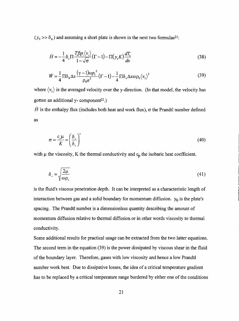
Q = roEst E

(43)

where Est is the energy stored in the resonance and E is the average rate of dissipation.

Est can be obtained by integrating the time averaged acoustic energy densitJ28 over the

volume of the resonator. E can be calculated by integrating thermal and viscous surface

dissipation over the whole surface of the resonator. Applied to the different geometries of

resonators, losses of the tapered tube are decreased by about 30% to the straight tube

resonator which diminishes the losses of the half wavelength resonator by about one half.

The resonator used in our experiments, ranks between the latter two.

28

CHAPTER 3: Experimental Setup and Construction

A. The Driver

The simplicity in the construction consists of the usage of a regular, though slightly

modified high fidelity midrange loudspeaker29. A speaker with high power capabilities

had to be chosen. This is realized by speaker with a ferrofluid in the magnet gap and the

voice coil wrapped around an aluminum cylinder. The main modification was the cutoff

of the soft dome membrane. Instead, an aluminum cone machined in a lathe with a

moving mass of2.2 grams was glued in place. It tapers from a diameter of 5.08 mm

where it is attached to the voice coil of the speaker down to 2.54 mm where the end is

closed with a slight taper and a small flat in the middle. The wall thickness is 0.3 mm.

This change was due to adapting the mechanical impedance, an expression for stiffness

(imaginary part) and damping (real part) of the driver, to the high acoustical impedance

of the fluid at this location. In other words, the cone had to withstand the comparatively

high dynamic pressure differential at the pressure antinode.

Another surround (a flexible connection between the cone and the housing) was made to

close up the upper end. It consisted of a rubber like gastight fabric. It was epoxied to the

cone where the slight taper starts and attached by screws and a washer to the driver's

housing. It is pushed somewhat together to allow the cone to move freely. The driver is

bolted to the machined aluminum housing and heat sink. A bore with the same taper as

the cone was machined to the end joining the resonator tube. After placing the speaker

into the housing, the surface of the housing and the cone were nearly level. The flat of

the cone stuck out slightly. Care was taken to make a good thermal connection between

the magnet and the housing to remove the excess heat. An aluminum lid with an 0-ring

29

closed the housing gastight from the top.

,-..

r • J;

.

Figure 7: Picture of the modified speaker with the aluminum cone replacing the soft dome

B. The Heat Exchangers

The heat exchangers were made from copper meshes soldered on a machine made groove

on the copper tube. Three screens have been used for the hot heat exchanger with a total

thickness of 2.4 mm and two for the cold heat exchanger with a total thickness of 1.6

mm. The screens were precisely aligned. The dimensions of the heat exchangers were

chosen to be different since the hot heat exchanger has to conduct much more heat than

the cold heat exchanger. Care was taken to establish a good thermal contact to the copper

tube for a good heat supply and removal.

30

C. The Stack

In contrast to the theoretical treatment, a spiral roll was used instead of a stack of parallel

plates. It consists of a approximately 250 cm long, 80 mm wide and 0.12 mm thick

flexible plastic strip. This strip is wound around a a plastic rod, that is 80 mm long and 8

mm in diameter. The spacers were made from regular 0.44 mm diameter fishing line. A

jig was machined with grooves on either side to glue and align the spacers both vertically

and parallel on the plastic strip.

: I I I

I I

I

I

1

I (

I I

i I

figure 8: String alignment jig and section of the plastic film

The fishing line was fastened by a bolt to one end, then laced back and forth by making

use of the grooves and then bolted to the other end. 10 lines could be glued to the strip at

the same time spaced 8 mm apart. After lacing the jig, a spray adhesive was applied to

one side of the string. A flat block fitting in the middle of the jig with a weight on it was

used to press the strings firmly on the plastic strip until it sticks. The strings were cut off

at the edge with a scalpel. Finally, the strip was wound tightly around the rod and pushed

into the tube with a piston.

31

Figure 9: Picture of the rolled up stack

D. The Resonator

The resonator consists of a quarter wavelength tube with a cylinder shaped volume at the

bottom.

For reasons of simplicity, the sphere and the neckdown (see figure 6d) were given up and

replaced by a straight tube and a cylinder. The tube can be divided into three parts. The

upper part containing the hot heat exchanger is made from copper to ensure good thermal

conduction. It is attached to the speaker housing by a flange. Some copper tubing is

wound and soldered to the flange with water flowing through to provide cooling for the

32

hot heat exchanger and the speaker. This upper part is epoxied into a plastic tube. This

second section contains the stack which is going to create and sustain the temperature

gradient. Hence, this should be made from thermally poor conducting material. In our

case this was section of Schedule 40 PVC pipe. The last section, a copper tube with the

cold heat exchanger on top is epoxied from the other side into the plastic tube making

contact between the stack and the heat exchanger. The other end of the tube is silver

soldered onto the aluminum can which is closed with copper lids from the top and the

bottom.

The cold section reaches from the cold heat exchanger to the very bottom. The large can

is kept in a snug fit polystyrene box for thermal insulation from the ambient. For the rest

of the cold portion, polystyrene housing was cut and placed tightly around it.

E. Vacuum and Helium

From the considerations in chapter 2.3 can be seen that helium as a working fluid is

desirable. In order to change the working fluid and the pressure in the refrigerator, a

vacuum system with a vacuum rotary pump and a helium pressure bottle had to be

installed. The helium bottle is equipped with a regulator and a pressure gauge to adjust

and measure the mean pressure in the tube. The housing and the resonator have to be

evacuated and filled at the same time since there is no gas connection between them. The

tubing is screwed and epoxied into the housing and resonator, respectively.

33

vacuum pump -t><J

helium

speaker housing

© en 0 :J 0 0 """'

LJ Figure 10: Drawing of the vacuum and helium filling system

F. Instrumentation and Measurements

Copper- constantan thermocouples were used for the temperature measurement. One end

of each thermocouple was soldered onto the hot and the cold heat exchanger,

respectively, directly on the middle of the copper screens. The wires are led through tiny

holes of the tube wall. Both holes are closed with a little drop of epoxy. The reference

end of the thermocouples was put in an ice- water bath in a dewar for a constant reference

temperature. The obtained voltage was amplified, measured with a multimeter and

converted to a temperature from the calibration curve shown in figure 11 of the

thermocouple's signal versus temperature.

34

u -~ Q)

~ 05 03 c... E Q)

I-

-0.8 -0.6 -0.4 -0.2

Thermovoltage in V

100

80

60

40

20

0

Figure 11: Calibration curve of the thermocouple in conjunction with an amplifier, with

one junction in an ice bath and the other junction in water

A pressure signal was obtained by using a quartz piezo crystal glued upright onto the hot

heat exchanger near the pressure antinode. The leads to the pressure transducer were

introduced through a hole in the wall as well. Basically, the transducer has been used to

verify the theoretical calculated resonance frequency experimentally. The resonance

frequency for a pipe can be determined by the following formula considering that it is a

quarter wavelength resonator.

f=~=l_ {Ji=J__~yRT 'A 'A ~P. 'A M

(44)

with 'A= 41+0.82r. 1 is the length and r the radius of the resonator. The second term is a

correction term3o.

35

G. Demonstration Tube

For demonstration purposes, a prime mover, a thermally driven oscillator has been made.

~ ··-6- .j___ - 1 -i- --6 _J

T 1.625

I

j_

L__ SCREEi'J --- ·······----_i

Figure 12: Drawing of a simple thermoacoustic oscillator

36

As soon as a sufficient large temperature gradient has been established, it begins to

oscillate spontaneously. Design and construction was kept quite simple and basically the

same methods as in the refrigerator were applied.

The core parts are the stack, the heat exchangers and the resonator. Two copper tubes of

equal length are used for the resonator. The same copper screens used for the heat

exchangers in the refrigerator are soldered onto one end of either tube, one on each side.

The stack has been made in the same way as the first one. However, the width is only

2.54 cm. It is housed in a plastic tube. The two copper tubes were stuffed into the plastic

housing until the screens make contact with the stack. One end was closed up by a

copper lid. The tube has a total length of 13 in.

In operation, the open end is immersed in liquid nitrogen with the liquid level close to the

heat exchanger and the closed end is kept warm by the hands. After a sufficient

temperature gradient has been established it starts to vibrate and shake and after taking it

out, it starts to release a sound.

37

CHAPTER 4: Experimental Results and Conclusions

4.1 Results

The pressure signal obtained by the pressure tranducer has been measured for verifying

the resonance frequency and determining the quality factor of the resonator.

The transducer turned out to work quite well. However, due to the high dynamic pressure

amplitude, the signal on the oscilloscope was not sinoidial but somewhat distorted. The

pressure signal of the transducer as a function of the frequency was measured for air and

helium as a working fluid. This is shown in figures 13 and 14. The resonance frequency

(where the signal of the pressure transducer is greatest) can be seen in table 3. Equation

( 44) has been used for calculating the theoretical value.

Table 3: Calculated and experimentally determined resonance frequency for T=20°C

medium Calculated by experimentally

equation (44)

air (fundamental 267 281

mode)

air (first mode 791 785

resonance)

Helium 762 805

38

5

4.5 .!!? 4 ·c: :::J

3.5 t ; \ I ~ • e • ±: \ • :e 3 0

2.5 t • -~ ~ ~· Q) ~. O> 2 0 +-g 1.5

1

0.5

0 0 100 200 300 400 500 600 700 800 900 1000

Frequency in Hz

Figure 13: Voltage signal of the pressure tranducer in arbitrary units as a function of the

frequency for air (p=l atm, T=20 °C)

.!!? ·c

3.5 T

3 + :::J ~ 2.5 t Q I ~ I :e 2 l c I C I _.

·a; 1.5~-~ O> .

J? ~

1

0.5

• •

~ ~~~

0 +-~~_._~~~t--~~-t-~~-+~~~-r-~~--~~~t--~----;

600 700 750 780 805 820 850 900 1100

frequency in Hz

Figure 14: Voltage signal of the pressure transducer in arbitrary units versus the

frequency for helium (p= 1 atm, T=20 °C)

With a power output from the amplifier of 9W, after 10 minutes the following

39

temperatures were measured with an ambient temperature of 20°C.

The temperature of the cold heat exchanger was l 6°C and the temperature of the hot heat

exchanger was 23 °C.

4.2 Conclusions

The objective of this research was to build a thermoacoustic refrigerator and analyzing its

basic performance.

The experimentally obtained resonance frequencies matched quite well with the

calculated values. The deviations were less than 5%. The two resonances in air, the

fundamental mode resonance ( t /...) and the first mode resonance ( t /...) can be seen quite

well.

The measured cooling effect was distinct, although quite small. According to the data

reputed on the Hofler refrigerator3, a much lower temperature along with a higher cooling

power would have been expected. The reasons for the comparatively poor performance

are various. The main reason was the limited amount of power which could be applied to

the speaker due to its repeated breakdowns. The voice coil and the surround came apart

at one side. Due to the relative motions between the voice coil and the surround and due

to the fact that the lead to the voice coil was in contact with the surround the lead broke

off. Several attempts to fix it permanently were not successful. It broke off repeatedly,

even though we ran it with minimal power (9W in comparison to an estimated 150W in

the Hofler's experiment). The cold section was designed to be fairly large. It was

comprised of the cold heat exchanger attached to the copper tube below as well as the

large volume at the bottom. The small amount of acoustic power that could be delivered

40

into the tube, was likely not enough to cool the entire section. The heat conduction in the

copper tube and the brass can would in addition hinder the cooling down of the cold heat

exchanger.

Finally, it can be said that we built a working acoustic refrigerator. For more elaborate

results and a comparison of theory and experiment, a new speaker has to be bought or

made. The instrumentation, such as the pressure transducer and accelerometer for

quantitative measurement of acoustic power have to be improved and/or installed.

41

References

1N. Rott, Adv. Appl. Mech. 20, 135 (1980).

2J. Wheatley, T. Hofler, ... "Understanding some simple phenomena in thermoacoustics

with applications to heat engines", Am. J. Phys. 53 (2), 148 (1985).

3Th. Hofler, Dissertation, "Thermoacoustic Refrigerator Design and Performance" (1986).

4P. Storch, R. Radebaugh, J. Zimmermann, "Analytical Model for the Refrigeration

Power of the Orifice Pulse Tube Refrigerator", Natl. Inst. Stand. Tech. 1343 (1990).

5Landau-Lifshitz, "Fluid Mechanics", Pergamon Oxford (1987), eqn. 64.9.

6ref. 5, eqn. 2.3.

7R. Sonntag, "Introduction to Thermodynamics", John Wiley & sons New York, eqn.

12.12.

sref. 7, eqn. 5 .15.

9ref. 7, eqn. 12.47.

IOref. 5, eqn. 49.4.

IIref. 7,eqn.12.14.

12G.W. Swift, "Thermoacoustic engines", J. of Acoustic Soc. Am. 84 (1988), 1164.

Bref. 7, eqn. 12. 7 for dP=O.

14Peter Leung, Lecture electrodynamics winter term 1994, Portland State University.

Isref 12, 1152.

I6ref 12, 1153.

17ref 12, 1156-1160.

I8ref. 5, eqn. 15.6.

19ref 12, 1176-1179.

20ref 5, eqn. 49.2.

21ref. 12, 1160.

42

22ref 1, 138.

23E. Verheiden, Handbook of Chemistry and Physics, 50th edition (1969), E3, E2, D125.

24ref. 23, F43.

25ref. 3, figures 1 and 2.

26S. Bate, "Acoustical and Vibration Physics", London Eduard Arnold LTD (1966) 277-8.

27ref. 12, 1162.

28ref. 5, eqn. 65.1.

29Midrange high fidelity loudspeaker, Dynaudio Skanderborg Denmark, model AF 3 5.

30ref. 26, 175.

43