Embed Size (px)
Citation preview

DEVELOPMENT OF SMALL-SCALE THERMOACOUSTIC ENGINE
AND THERMOACOUSTIC COOLING DEMONSTRATOR
By
NAJMEDDIN SHAFIEI-TEHRANY
Masters in Mechanical Engineering
Washington State University School of Mechanical and Material Engineering
May 2008
ii
To the Faculty of Washington State University
The members of the Committee appointed to examine the thesis of Najmeddin
Shafiei-Tehrany find it satisfactory and recommend that it be accepted.
________________________________ Chair
________________________________
________________________________

iii
Acknowledgements
Many special thanks go to my advisor, Dr. Konstantin Matveev, for the guidance he gave
me during my graduate studies. Without his help and patience I would not have succeeded. I also
extend my gratitude to Mr. John Rutherford, machinist at The Science Shop, and Mr. Kurt
Hutchinson, machinist at The Mechanical and Materials Engineering Shop, for their
professionalism and the time they spent on manufacturing the components of the thermoacoustic
engine and the refrigeration system. I am also grateful for the assistance provided by Mr. Robert
Lentz during the entire research. I also would like to thank the Mechanical Shop for allowing me
to use their machines to manufacture necessary parts at my convenience. I also would like to
thank Dr. Mike Anderson for all the help and support he showed throughout my research. Finally
I would like to thank my committee, Prof. Robert Richards and Prof. Cecilia Richards, for
honoring me with their participation.
iv
Development of Small-Scale Thermoacoustic Engine and Thermoacoustic Cooling Demonstrator
Abstract
By Najmeddin Shafiei-Tehrany, M.S. Washington State University
May 2008
Chair: Konstantin Matveev
Thermoacoustics is a science and technology field that studies heat and sound
interactions. Sound waves in any fluid consist of coupled pressure, motion, and temperature
oscillations. When the sound travels through a narrow channel, an oscillating heat flow between
the fluid and the channel’s wall becomes significant. The present study deals with the effects of
thermoacoustic cooling with closed and open ended tubes and also investigates the performance
of a small-scale thermoacoustic heat engine.
The first part of this document presents the design, construction, and testing of a
miniature standing-wave thermoacoustic heat engine. The main objective was to build and test a
miniature heat engine without moving parts. Recorded parameters included the temperature
difference across the stack and the corresponding acoustic pressure amplitude of the sound
produced by the engine. The system was also tested for different stack materials and tube
lengths. The most efficient system is described in detail in this document. The critical
temperature difference across the stack was measured to be approximately 350°C for the 5.8 cm
engine and 250°C for the 9.3 cm engine. The average acoustic RMS pressure of the sound
produced was about 2.7 Pa at 30 cm from the engine for both lengths and the frequency of the
sound was about 1.4 kHz for the 5.8 cm engine and about 1 kHz for the 9.3 cm engine.
The second part of this document presents the effects of thermoacoustic cooling with
closed and open ended tubes. The position of the stack and sound frequencies were varied to
v
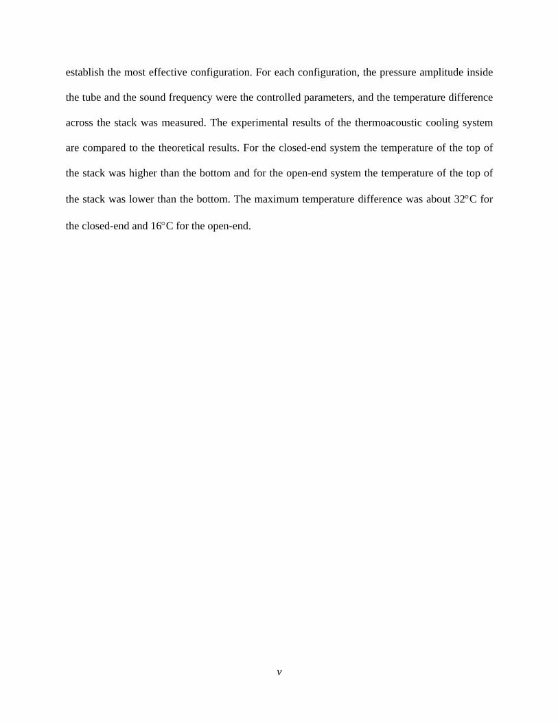
establish the most effective configuration. For each configuration, the pressure amplitude inside
the tube and the sound frequency were the controlled parameters, and the temperature difference
across the stack was measured. The experimental results of the thermoacoustic cooling system
are compared to the theoretical results. For the closed-end system the temperature of the top of
the stack was higher than the bottom and for the open-end system the temperature of the top of
the stack was lower than the bottom. The maximum temperature difference was about 32°C for
the closed-end and 16°C for the open-end.
vi
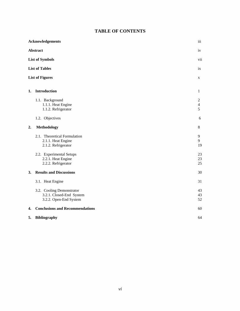
TABLE OF CONTENTS Acknowledgements iii Abstract iv List of Symbols vii List of Tables ix List of Figures x 1. Introduction 1
1.1. Background 2
1.1.1. Heat Engine 4 1.1.2. Refrigerator 5
1.2. Objectives 6
2. Methodology 8
2.1. Theoretical Formulation 9
2.1.1. Heat Engine 9 2.1.2. Refrigerator 19
2.2. Experimental Setups 23
2.2.1. Heat Engine 23 2.2.2. Refrigerator 25
3. Results and Discussions 30
3.1. Heat Engine 31
3.2. Cooling Demonstrator 43
3.2.1. Closed-End System 43 3.2.2. Open-End System 52
4. Conclusions and Recommendations 60 5. Bibliography 64
vii
List of Symbols
a speed of sound pc isobaric heat capacity per unit mass
D diameter of the stack hxD diameter of the heat exchanger
h spacing between the stack plates hxh spacing between the heat exchanger plates
k fluid thermal diffusivity K fluid thermal conductivity
SK solid thermal conductivity l stack’s plate half-thickness hxl heat exchanger’s plate half-thickness L resonator length
sp acoustic pressure waveform
AP acoustic pressure amplitude R radius of the resonator
gR air gas constant
mT mean temperature
mT∇ mean temperature gradient across the stack
critT∇ ideal critical temperature gradient across the stack TΔ temperature difference across the stack su acoustic velocity waveform
x coordinate along the resonator Sx stack position xΔ stack length
hxxΔ heat exchanger length
0y half-spacing between plates of the stack
hxy0 half-spacing between plates of the heat exchanger γ ratio of specific heats
sε stack’s plate heat capacity ratio σ Prandtl number Γ normalized temperature gradient Π cross-sectional perimeter of the stack surface
hxΠ cross-sectional perimeter of the heat exchanger surface ω angular frequency
radλ radian wavelength
viii
λ acoustic wavelength β thermal expansion coefficient
mρ mean density ν kinetic viscosity μ dynamic viscosity
kδ thermal penetration depth of the fluid
sδ thermal penetration depth of the solid material
νδ viscous penetration depth of the fluid
ix
List of Tables
1. Tabulated Temperature Uncertainty Calculations 33
2. Tabulated Temperature Uncertainty Calculations 33
3. Tabulated Results of the Acoustic Pressure RVC 100 PPI 39
4. Tabulated Results of the Acoustic Pressure for RVC 80 PPI 40
5. Tabulated Results of the Acoustic Pressure for Steel Wool 40
6. Pressure Uncertainty Calculations for 5.8 cm Engine at Different Angles 41
7. Tabulated experimental and theoretical results for both 5.8 and 9.3 cm engines 42
8. Uncertainty Calculations for Different RMS Pressures 49
9. Uncertainty Calculations for Different Stack Positions 49
10. Uncertainty Calculations for Different Stack Positions 57
11. Uncertainty Calculations for Different RMS Pressures 58
x
List of Tables
1. Two Types of Heat Engine 3
2. (a) Schematic of Thermoacoustic Engine 9 (b) Expanded View of the Stack Plates 9 (c) Pressure and Velocity Waveforms along the Resonator 9
3. Locations of Recorded Temperatures and Refrigerator Setting 21
4. (a) Schematic of 5.8 cm Engine 24 (b) Schematic of 5.8 cm Engine 24
5. Engine Structure 24
6. (a) Assembled 9.3 cm Engine With Cooling Jacket 24 (b) Photo of the 5.8 cm Engine 24
7. Heat Engine Experiment 26
8. (a) Schematic of Open-End System 27 (b) Schematic of Closed-End System 27
9. (a) Open-End System 28 (b) Closed-End System 28
10. (a) Open-Ended Refrigerator 29 (b) Closed-Ended Refrigerator 29
11. Temperature Profile for 5.8 cm Engine 31
12. Pressure Profile for 5.8 cm Engine 32
13. Variation of Temperature Difference for 5.8 cm Engine 32
14. Pressure Variation for 5.8 cm Engine 32
15. Acoustic RMS Pressure with the Change in Temperature Difference Across the Stack 34
16. Temperature Profile for Steel Wool 35
17. Temperature Profile for RVC 100 PPI 35
18. Temperature Profile for RVC 80 PPI 35

xi
19. Temperature Difference for RVC 100 PPI, 80 PPI, and Steel Wool for 5.8 cm Engine 36
20. Temperature Profile for 5.8 cm and 9.3 cm Engine with RVC 100PPI 39
21. Acoustic Pressure Profile for 5.8 cm and 9.3 cm engine with RVC 100PPI 39
22. Acoustic Pressure Error Measurements at Different Angles for 5.8 cm Engine 41
23. Frequency Profile for Stack at 13 cm 44
24. Temperature Difference for Stack Located at 7 cm 45
25. Temperature Difference for Stack Located at 9 cm 45
26. Temperature Difference for Stack Located at 11 cm 45
27. Temperature Difference for Stack Located at 13 cm 46
28. Temperature Difference for Different Stack Location at 3.5 kPa of RMS Pressure 46
29. Temperature Difference for Different Stack Location at 218 Hz 47
30. Repeatability Error for 218 Hz Signal and 3.5 kPa of RMS Pressure 48
31. Repeatability Error for 218 Hz Signal and Stack at 13 cm 48
32. Temperature Difference for Different Stack Material at 13 cm 50
33. Temperature Profile Recorded Every 15 Seconds 50
34. Temperature Profile Recorded Every 5 Seconds 51
35. Enthalpy Flow Across the Tube for a Close-Ended System 52
36. Temperature Difference for Stack Located at 6 cm 53
37. Temperature Difference for Stack Located at 7 cm 53
38. Temperature Difference for Stack Located at 8 cm 53
39. Frequency Profile for Stack at 6 cm 54
40. Enthalpy Flow Across the Tube for an Open-Ended System 55

xii
41. Temperature Difference for Different Stack Position at 0.35 kPa of RMS Pressure 55
42. Temperature Difference for Different Stack Position at 330 Hz 56
43. Repeatability Error for 330 Hz Signal and 0.5 kPa of RMS Pressure 56
44. Repeatability Error for 330 Hz Signal and Stack at 6 cm 57
45. Temperature Difference for Different Stack Material at 6 cm 58

1
Chapter 1
Introduction
2
Introduction
1.1. Background
Thermoacoustics is a science and technology field that studies heat and sound
interactions. Sound waves in any fluid consist of coupled pressure, motion, and
temperature oscillations. When sound travels through a narrow channel, an oscillating
heat flow between the fluid and the channel’s wall becomes significant. Devices in which
heat-sound interactions play an important role are known as thermoacoustic systems [1].
Audible sound temperature fluctuations are usually very small and normally not
important. In the case of thermoacoustic engines, the combination of temperature
gradient and special system geometry makes these temperature fluctuations important,
since they can significantly amplify sound [2].
Thermoacoustic effects have been studied since the 19th century. One of the first
observations was made in 1850 when Sondhauss recorded sound appearance in
glassblower equipment [3]. The sound waves were produced when hot glass came in
contact with a cool open ended glass tube. The frequency of the observed tonal sound
was equal to the natural frequency of the tube [4]. Subsequently, other thermoacoustic
findings soon followed. In 1859, Rijke noticed that placing hot gauze in the lower half of
an open-ended tube created a similar pure tone where sound oscillations were varied by
changing the gauze location along the tube. Rijke postulated that the expansion of air at
the gauze and the contraction of cooling air toward the open end of the tube explained the
sound generation [5]. Soon after these discoveries, Lord Rayleigh came up with an
explanation of the thermoacoustic instabilities which caused this phenomenon: “If heat be
given to the air at the moment of greatest condensation, or be taken from it at the moment

3
of greatest rarefaction, the vibration is encouraged. On the other hand, if heat be given at
the moment of greatest rarefaction, or abstracted at the moment of greatest condensation,
the vibration is discouraged” [6].
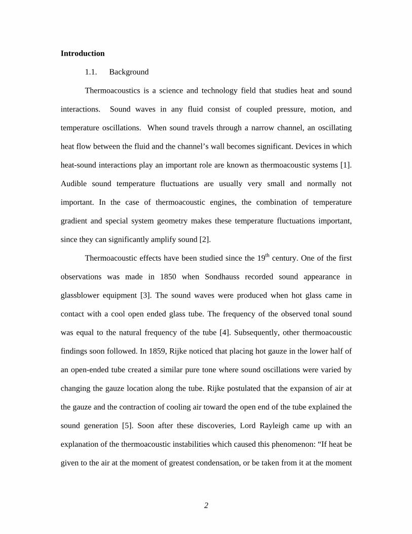
Thermoacoustic devices can be made without moving parts and using various
gases as working fluids. The simplicity of manufacturing such engines results in low cost
and low maintenance and, therefore, is desirable in industry [7]. Thermoacoustic engines
can be divided into two major groups. In the first group, thermoacoustic prime movers
convert some fraction of heat supplied from a high temperature source into acoustic
power, rejecting the rest of the heat into a low temperature heat sink. In the second group,
thermoacoustic refrigerators and heat pumps use sound to pump heat against a
temperature gradient. The temperature gradient in a refrigerator is typically much lower
than in the heat engine [16]. Figure 1 shows the two basic types of heat engines.
Figure 1: Two types of heat engine.
There have been major developments and advances in the thermoacoustic field in recent
decades and some thermoacoustic systems have been tested for industrial use. One
example is large scale commercial refrigeration using thermoacoustic engines. The
efficiency limitations in simple standing wave engines motivated the development of
closed loop traveling wave engines, a few meters in size, that produce approximately 1
kW of acoustic power [13]. Other medium-scale systems were built that produce up to
WQ
T
TH
C
H
QC
..
.Engine
Prime Mover
W Q
T
TH
C
H
QC
. .
.Engine
Heat Pump - Refrigerator
4
100 W of acoustic power. One example of such a thermoacoustic engine was built by
NASA with a total length of 16 cm and weight of about 900 g [12].
Because manufacturing macro-scale thermoacoustic engines is relatively simple,
most of the work and studies done use large or medium engines. Some of the
thermoacoustic projects are aimed at converting acoustic power into electric power. A
project attempting to facilitate this conversion was originally designed for a space
generator which produced 100 W of electrical power at 20% efficiency. This engine has
a total length of 16 cm, but the generated power is much larger in comparison to previous
designs [14]. Another case study was done at Los Alamos National Laboratory that
coupled a thermoacoustic engine to an electric alternator, which was part of a NASA
space project [16].
1.1.1. Heat Engine
A simple thermoacoustic engine consists of a tube (resonator) with one end closed
and the other end open to the atmosphere with a porous material, referred to as a stack,
placed inside the tube at a fixed location. The system produces sound only when the
temperature difference across the stack exceeds a critical value. Thermoacoustic heat
engines can be divided in two major categories: standing-wave and traveling-wave
engines. In a standing-wave thermoacoustic heat engine, heat is supplied to the oscillating
gas at high pressure and is removed at a low pressure supporting pressure and velocity
fluctuations. These self-sustained oscillations satisfy Rayleigh’s criterion; in other words,
heat is added to the gas in phase with pressure fluctuations, similar to the Stirling cycle
[16]. For thermoacoustic pumps or refrigerators this process is reversed.
5
In a traveling-wave heat engine, the pressure and velocity components of an
acoustic traveling wave are inherently phased to cause the fluid in the stationary
temperature gradient to undergo a Stirling thermodynamic cycle. This cycle results in
amplification or attenuation of the wave depending on the wave direction relative to the
direction of the gradient. This cycle pumps heat in the direction opposite the direction of
wave propagation through the device [9].
Various thermoacoustic systems have been built in the past, usually in large or
medium scale. The main motivation for our research is to build a miniature engine with a
relatively simple design for ease of manufacturing. An example of a relatively small
thermoacoustic engine previously developed is a 14 cm Hofler tube [7]. The Hofler tube
has a constant bore capped at one end, and similar to other engines, open on the other
end. The open end is made of aluminum and funnel shaped with a stack of reticulated
vitreous carbon (RVC). Smaller engines, down to few centimeters in length, were also
built [17], but their design was not documented in details sufficient for reproduction.
1.1.2. Refrigerator
A simple thermoacoustic refrigerator consists of a resonator with one end attached
to a speaker. The other end is open or closed, and porous material (stack) is placed at a
certain location inside the resonator [6]. The stack usually consists of a large number of
closely spaced surfaces aligned with the resonator tube. The primary constraint in
selecting the stack is the fact that stack layers need to be placed a few thermal penetration
depths apart. About four thermal penetration depths is the recommended plate separation
in standing-wave systems. Thermal penetration depth is the distance, or thickness, of the
6
layer where unsteady heat propagates during one oscillation cycle [1]. In a refrigerator,
externally applied work transfers heat from the lower temperature reservoir to the higher
temperature reservoir. In this case the external work is supplied by the standing sound
wave produced by a speaker in the resonator. The standing sound wave forces the gas
particles to oscillate parallel to the walls of the stack. The alternating compression and
rarefaction of the gas causes the local temperature of the gas to fluctuate. If the local
temperature of the gas becomes higher than that of the nearby stack wall, heat is
transferred from the gas to the stack wall. However, if the local temperature of the gas
drops below that of the stack wall, heat is transferred from the wall to the gas. Depending
on the system’s configuration, the mean temperature of each stack end will differ. In the
closed-end configuration, the temperature of the stack end close to the cap is higher than
the other end of the stack, where a cooling effect is achieved. The heat is pumped from
the cold end to the hot end.
1.2. Objectives
The main objective of this study is to build and test a miniature thermoacoustic
engine and quantify its performance. The development process included several different
models that were built and tested. The heat engine was tested with different stack
materials in order to find the best material for the stack. The values measured in our
studies are the critical temperature across the stack and the pressure amplitude of the
sound produced. These values are compared with theoretical values obtained from
numerical analysis.
7
The second part of our efforts deals with a construction of a cooling model with a
speaker as a sound source. This system is built and then tested with different stack
materials and two different geometry configurations: closed- and open-ended. The
frequency of the acoustic signal and the pressure amplitude inside the resonator were
controlled parameters, and the measured parameter was the temperature difference across
the stack. These studies are done to identify the differences between a closed and open
systems and also to find the most effective system. The experimental results were
compared with the theoretical values. Some results of these activities were presented at
conferences [18, 19].

8
Chapter 2
Methodology
9
2. Methodology
2.1. Theoretical Formulation
2.1.1. Heat Engine
The goal of this section is to theoretically obtain the critical temperature
difference across the stack, the acoustic power produced, and the acoustic pressure
amplitude. In order to formulate necessary equations to calculate these parameters, the
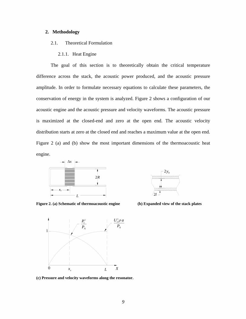
conservation of energy in the system is analyzed. Figure 2 shows a configuration of our
acoustic engine and the acoustic pressure and velocity waveforms. The acoustic pressure
is maximized at the closed-end and zero at the open end. The acoustic velocity
distribution starts at zero at the closed end and reaches a maximum value at the open end.
Figure 2 (a) and (b) show the most important dimensions of the thermoacoustic heat
engine.
Figure 2. (a) Schematic of thermoacoustic engine (b) Expanded view of the stack plates
(c) Pressure and velocity waveforms along the resonator.
X sx
1
L
A
s
PP1
0
A
s
PaU ρ1
l2
02y
L
x Δ
R2
xs
10
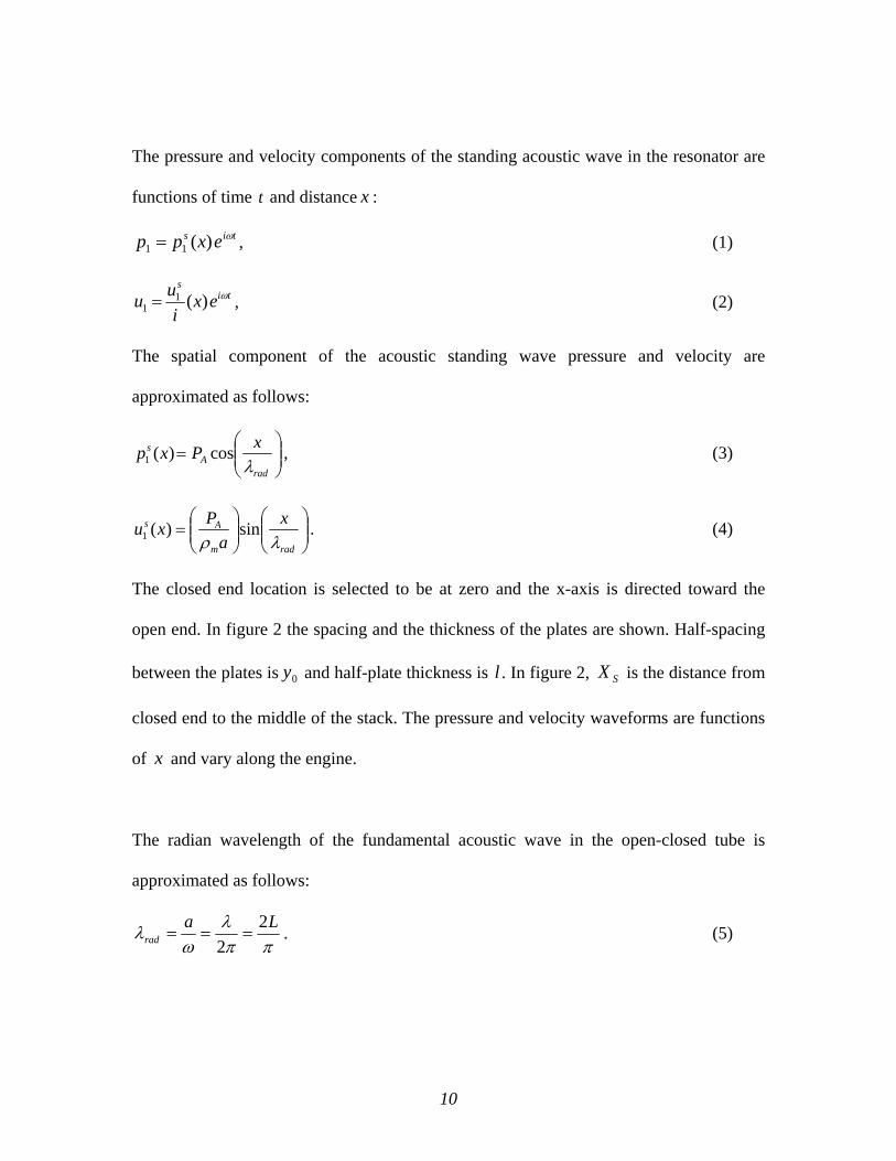
The pressure and velocity components of the standing acoustic wave in the resonator are
functions of time t and distance x :
tis expp ω)(11 = , (1)
tis
exi
uu ω)(11 = , (2)
The spatial component of the acoustic standing wave pressure and velocity are
approximated as follows:
⎟⎟⎠
⎞⎜⎜⎝
⎛=
radA
s xPxpλ
cos)(1 , (3)
⎟⎟⎠
⎞⎜⎜⎝
⎛⎟⎟⎠
⎞⎜⎜⎝
⎛=
radm
As xa
Pxuλρ
sin)(1 . (4)
The closed end location is selected to be at zero and the x-axis is directed toward the
open end. In figure 2 the spacing and the thickness of the plates are shown. Half-spacing
between the plates is 0y and half-plate thickness is l . In figure 2, SX is the distance from
closed end to the middle of the stack. The pressure and velocity waveforms are functions
of x and vary along the engine.
The radian wavelength of the fundamental acoustic wave in the open-closed tube is
approximated as follows:
ππλ
ωλ La
rad2
2=== . (5)

11
The wavelengthλ is a function of length of the resonator. In our case, since one end of
the engine is open, the wave length is equal to about L4 . The speed of sound is a
function of temperature and for ideal gas can be written as follows:
TRa γ= , (6)
where T is the gas temperature.
Therefore the natural frequency of the open-closed tube becomes a function of
temperature and tube length:
LTR
f42γ
πω
== , (7)
In order to find the critical temperature difference across the stack we use the energy
balance of the system [3]:
hxresrad EEEW &&&& ++=2 , (8)
where 2W& is the acoustic power produced, radE& is the radiated acoustic power, resE& is the
acoustic power absorbed by the walls of the resonator, and hxE& is the acoustic power
absorbed by thermoviscous effects in heat exchangers.
Acoustic oscillations occurring in the vicinity of a plate result in two important effects:
the generation and absorption of acoustic power 2W& , and also a time-average heat flow
2Q& near the surface of the plate, both effects occurring along the direction of acoustic
oscillation.
Now each term in the energy balance equation will be analyzed. The acoustic power
produced in the presence of thermoviscous losses can be written as follows [3]:
12
( ) ( )( ) ( )
( )( )2
0
2
0
21
20
2
0
2
21
2
21
411
211
1)(1
41
yy
xux
yya
xpxW ss
mv
sm
Ss
kνννν δδ
ωρδδδσ
ερωγδ
+−ΔΠ−
⎟⎟⎟⎟⎟
⎠
⎞
⎜⎜⎜⎜⎜
⎝
⎛
−
⎟⎟⎠
⎞⎜⎜⎝
⎛+−+
Γ⎟⎟⎠
⎞⎜⎜⎝
⎛
+−
ΔΠ=& , (9)
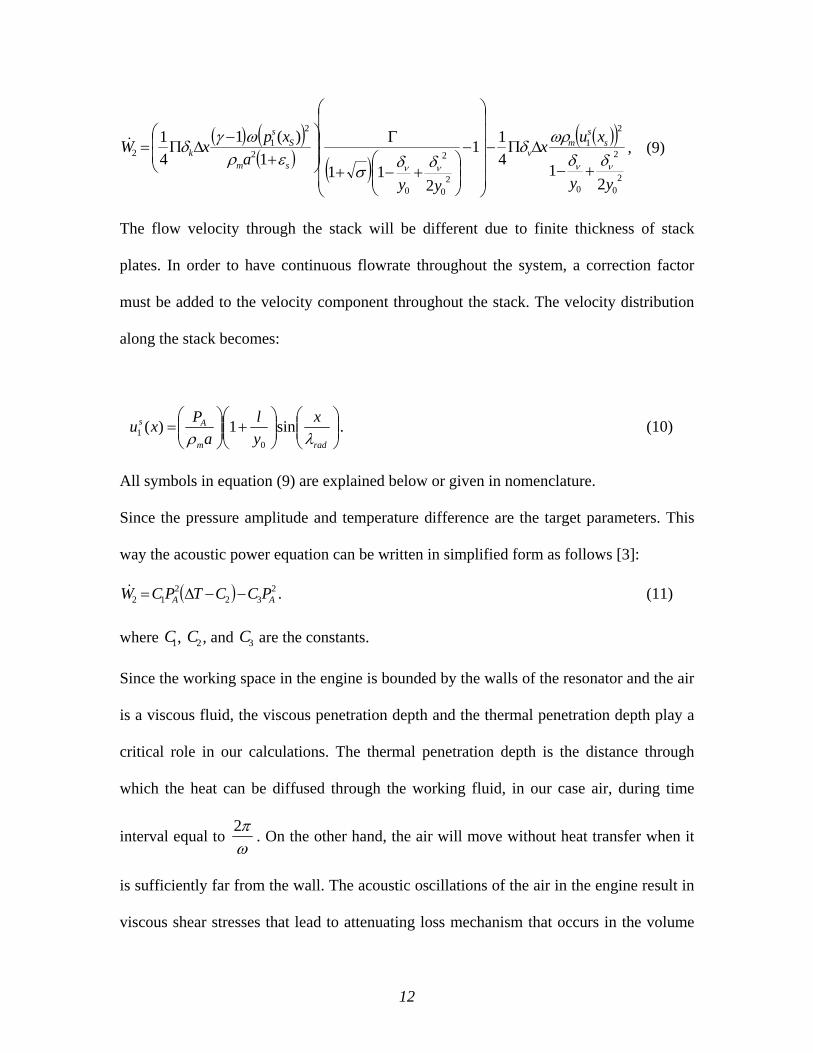
The flow velocity through the stack will be different due to finite thickness of stack
plates. In order to have continuous flowrate throughout the system, a correction factor
must be added to the velocity component throughout the stack. The velocity distribution
along the stack becomes:
⎟⎟⎠
⎞⎜⎜⎝
⎛⎟⎟⎠
⎞⎜⎜⎝
⎛+⎟⎟
⎠
⎞⎜⎜⎝
⎛=
radm
As xyl
aPxu
λρsin1)(
01 . (10)
All symbols in equation (9) are explained below or given in nomenclature.
Since the pressure amplitude and temperature difference are the target parameters. This
way the acoustic power equation can be written in simplified form as follows [3]:
( ) 232
212 AA PCCTPCW −−Δ=& . (11)
where 1C , 2C , and 3C are the constants.
Since the working space in the engine is bounded by the walls of the resonator and the air
is a viscous fluid, the viscous penetration depth and the thermal penetration depth play a
critical role in our calculations. The thermal penetration depth is the distance through
which the heat can be diffused through the working fluid, in our case air, during time
interval equal to ωπ2 . On the other hand, the air will move without heat transfer when it
is sufficiently far from the wall. The acoustic oscillations of the air in the engine result in
viscous shear stresses that lead to attenuating loss mechanism that occurs in the volume
13
of air generally within a viscous penetration depth. The viscous penetration depth in the
fluid can be written as follows:
ωνδν
2= , (12)
where kinematic viscosity is:
mρμν = . (13)
Here the mean density mρ is a function of temperature that for the ideal gas becomes:
TRP
gm =ρ , (14)
where for air Kkg
kJRg 287.0= .
The dynamic viscosity of the working fluid, in our case the air, also varies with
temperature [3].
The thermal penetration depth of the solid is
ωδ k
k2
= , (15)
where thermal diffusivity is
pmcKk
ρ= . (16)
The Prandtl number is one of the parameters used, which can be written as:
2
⎟⎟⎠
⎞⎜⎜⎝
⎛===
k
p
kKc
δδνμ
σ ν . (17)
14
The plate heat capacity ratio sε uses the properties of the fluid, in our case the air, and the
properties of the solid. Considering ky δ>>0 and sl δ>> , the simplified expression for sε
is:
solidsss
airkpm
s ccδρδρ
ε = , (18)
The perimeter in equation (9) can be approximated assuming parallel plate stack
geometry:
hD2
2π=Π , (19)
where 02yh = , if 0yl << , or with the finite plate thickness, 00 22 lyh += .
The next term that appears in the equation is the normalized temperature gradient.
Normalized temperature gradient is the ratio of to the actual and ideal critical temperature
gradient.
crit
m
TT
∇∇
=Γ , (20)
where f∇ is defined as dxdf since we consider a one-dimensional problem.
In this case mT∇ is the mean temperature gradient of the tube in the x-direction, which
can be represented as follows:
xTTm Δ
Δ=∇ , (21)
where TΔ is the difference temperature of two sides of the stack and xΔ is the stack
length.
15
The critT∇ is the critical mean temperature gradient that can be obtained using the
following equation [3]:
( )ss
pm
Ss
mcrit xuc
xpTT
1
1 )(ρβω
=∇ . (22)
The thermal expansion coefficientβ for an ideal gas is
T1
=β . (23)
Now we consider individual terms on the right hand side of equation (8).
The first term is the radiated acoustic power radE& . The acoustic power radiating away
from the open end of a small-diameter 4λ
resonator [1]:
⎟⎟⎠
⎞⎜⎜⎝
⎛⎟⎠⎞
⎜⎝⎛= 2
42
8 radm
Arad a
RPEλρ
π& , (24)
Where AP is the acoustic pressure amplitude at the closed end of the resonator and R is
the radius of the resonator. The simplified form of radiated acoustic power is:
24 Arad PCE =& , (25)
where
⎟⎟⎠
⎞⎜⎜⎝
⎛= 2
43
4 32 aLRCmρ
π . (26)
Acoustic power adsorbed by the resonator walls resE& is obtained by integrating the local
power attenuation per surface area over 4λ of side walls:
( ) ( ) ( ) ωδρε
γωρ
δν
212
21
41
11
4s
msm
sk
res ua
pe +
+−
=& , (27)
16
where sp1 and su1 were defined by equation (3) and (4).
We integrate rese& over the surface area of the resonator.
( ) 02
0 res e2e &&& RdxREL
res ππ += ∫ . (28)
Performing the integration we obtain:
⎟⎟⎠
⎞⎜⎜⎝
⎛+⎟
⎠⎞
⎜⎝⎛ +
+−
⎟⎟⎠
⎞⎜⎜⎝
⎛= νδδ
εγ
ρπω
LR
aPRLE k
sm
Ares 1
11
4 2
2& . (29)
The simplified equation of the acoustic power adsorbed is:
25 Ares PCE =& , (30)
where
⎟⎟⎠
⎞⎜⎜⎝
⎛+⎟
⎠⎞
⎜⎝⎛ +
+−
⎟⎟⎠
⎞⎜⎜⎝
⎛= νδδ
εγ
ρπω
LR
aRLC k
sm
11
14 25 . (31)
We obtain the acoustic power absorbed by viscous effects in the heat exchanger hxE& by
using the same equation that the acoustic power absorbed but this time it will be
multiplied the surface area of the first and the second heat exchanger.
Acoustic power absorbed:
( ) ( ) ( ) hxhxs
msm
sk
hx xua
pE ΔΠ
⎥⎥⎦
⎤
⎢⎢⎣
⎡+
+−
= ωδρε
γωρ
δν
212
21
41
11
4& , (32)
where the surface area can be expressed as follows:
hxhxhx
hxhx
hx
hxhxhx x
lyD
xhD
x Δ+
=Δ=ΔΠ222 0
22 ππ. (33)
In this case the pressure and velocity amplitude can be estimated from equations (3) and
(4) at heat exchanger locations.
The total energy absorbed by both heat exchangers (on each side of stack) is:

17
21 hxhxhx EEE &&& += , (34)
Finally the energy absorbed by the heat exchangers can be written as follows:
26 Ahx PCE =& , (35)
where
( )⎥⎦
⎤⎢⎣
⎡+
+−ΔΠ
= νδεγδ
ρω BA
axC
s
k
m
hxhx
11
4 26 , (36)
where A and B are parameters that include the acoustic pressure and velocity:
⎟⎟⎟⎟
⎠
⎞
⎜⎜⎜⎜
⎝
⎛⎟⎠⎞
⎜⎝⎛ Δ
++
⎟⎟⎟⎟
⎠
⎞
⎜⎜⎜⎜
⎝
⎛⎟⎠⎞
⎜⎝⎛ Δ
−=
L
xx
L
xxA
ss
22cos
22cos 22
ππ, (37)
⎟⎟⎟⎟
⎠
⎞
⎜⎜⎜⎜
⎝
⎛⎟⎠⎞
⎜⎝⎛ Δ
++
⎟⎟⎟⎟
⎠
⎞
⎜⎜⎜⎜
⎝
⎛⎟⎠⎞
⎜⎝⎛ Δ
−=
L
xx
L
xxB
ss
22sin
22sin 22
ππ. (38)
Combining equations (11), (25), (30), and (35) the critical temperature difference across
the stack TΔ can be written as follows:
21
6543 CC
CCCCT ++++
=Δ . (39)
It is important to note that the temperature difference is a function of geometry and
material property of the stack. Material properties relates to thermo-physical properties of
the materials used in the stack (air, copper, stainless steel). The geometries relate to the
resonator length L and radius R , stack position x and length xΔ , plate thickness l2 and
spacing 02y , and heat exchanger thickness hxl2 , spacing hxy2 , and length hxxΔ .
18
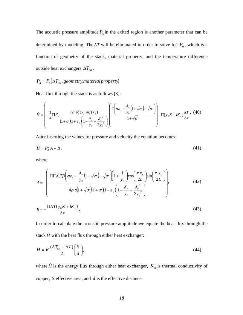
The acoustic pressure amplitude AP in the exited region is another parameter that can be
determined by modeling. The TΔ will be eliminated in order to solve for AP , which is a
function of geometry of the stack, material property, and the temperature difference
outside heat exchangers extTΔ .
( )propertymaterialgeometryTPP extAA ,,Δ=
Heat flux through the stack is as follows [3]:
( )( )
( )( )
xTlKKy
y
yy
xuxpTH s
vs
s
Ss
Ss
v ΔΔ
+Π−
⎟⎟⎟⎟⎟
⎠
⎞
⎜⎜⎜⎜⎜
⎝
⎛
+
⎟⎟⎠
⎞⎜⎜⎝
⎛−+−Γ
⎟⎟⎟⎟⎟
⎠
⎞
⎜⎜⎜⎜⎜
⎝
⎛
⎟⎟⎠
⎞⎜⎜⎝
⎛+−++
Π−= 00
20
2
0
11
1
1
2111
)()(41
σ
σσδ
σε
δδεσ
βδ
νν
& , (40)
After inserting the values for pressure and velocity the equation becomes:
BAPH A += 2& . (41)
where
( )
( )( )( ) ⎟⎟⎟⎟⎟
⎠
⎞
⎜⎜⎜⎜⎜
⎝
⎛
⎟⎟⎠
⎞⎜⎜⎝
⎛+−+++
⎟⎠
⎞⎜⎝
⎛⎟⎠
⎞⎜⎝
⎛⎟⎟⎠
⎞⎜⎜⎝
⎛+⎟⎟
⎠
⎞⎜⎜⎝
⎛−+−ΠΓ
−=
20
2
0
00
211114
2sin
2cos11
yya
Lx
Lx
yl
yT
A
s
ssvsv
νν δδεσσρ
ππσσ
δσεβδ
, (42)
( )x
lKKyTB s
Δ+ΠΔ
−= 0 , (43)
In order to calculate the acoustic pressure amplitude we equate the heat flux through the
stack H& with the heat flux through either heat exchanger:
⎟⎠⎞
⎜⎝⎛Δ−Δ
=dSTTKH ext
2)(& , (44)
where H& is the energy flux through either heat exchanger, cuK is thermal conductivity of
copper, S effective area, and d is the effective distance.
19
These parameters can be estimated as follows:
42hxhx DR
d == , (45)
hxhx xlnS Δ= 2 , (46)
where
( )hxhx
hx
ylR
n0+
=π
. (47)
The heat flow through the heat exchanger can now be written as:
( )TTCH exthx Δ−Δ=& , (48)
where
hx
hxhxcu
DxlnK
CΔ
=4
. (49)
Pressure amplitude can be calculated equating the heat transfer equations:
( )A
BTTCP ext
A−Δ−Δ
= . (50)
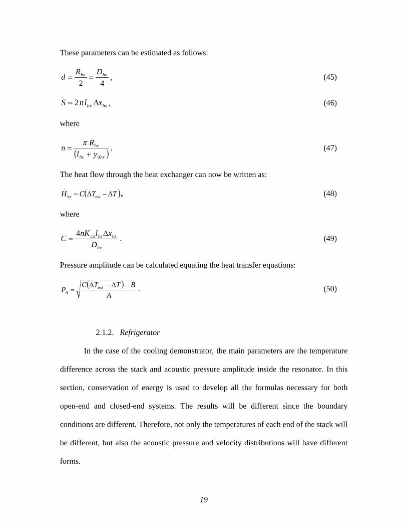
2.1.2. Refrigerator
In the case of the cooling demonstrator, the main parameters are the temperature
difference across the stack and acoustic pressure amplitude inside the resonator. In this
section, conservation of energy is used to develop all the formulas necessary for both
open-end and closed-end systems. The results will be different since the boundary
conditions are different. Therefore, not only the temperatures of each end of the stack will
be different, but also the acoustic pressure and velocity distributions will have different
forms.
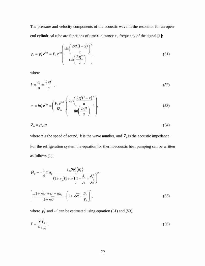
20
The pressure and velocity components of the acoustic wave in the resonator for an open-
end cylindrical tube are functions of time t , distance x , frequency of the signal [1]:
( )
⎟⎟⎟⎟
⎠
⎞
⎜⎜⎜⎜
⎝
⎛
⎟⎠⎞
⎜⎝⎛
⎟⎠⎞
⎜⎝⎛ −
==
afl
axlf
ePepp tiA
tis
π
πωω
2sin
2sin11 , (51)
where
af
ak πω 2
== , (52)
( )
⎟⎟⎟⎟
⎠
⎞
⎜⎜⎜⎜
⎝
⎛
⎟⎠⎞
⎜⎝⎛
⎟⎠⎞
⎜⎝⎛ −
⎟⎟⎠
⎞⎜⎜⎝
⎛==
afl
axlf
iZePeiuu
tiAtis
π
πω
ω
2sin
2cos
011 , (53)
aZ airρ=0 , (54)
where a is the speed of sound, k is the wave number, and 0Z is the acoustic impedance.
For the refrigeration system the equation for thermoacoustic heat pumping can be written
as follows [1]:
( )( )×
⎟⎟⎠
⎞⎜⎜⎝
⎛+−++
Π−=
20
2
0
112
11141
yy
upTH
s
ssm
kνν δδσε
βδ&
⎥⎦
⎤⎢⎣
⎡⎟⎟⎠
⎞⎜⎜⎝
⎛−+−
++++
Γ0
11
1y
s νδσσ
σεσσ , (55)
where sp1 and su1 can be estimated using equation (51) and (53),
crit
m
TT
∇∇
=Γ , (56)
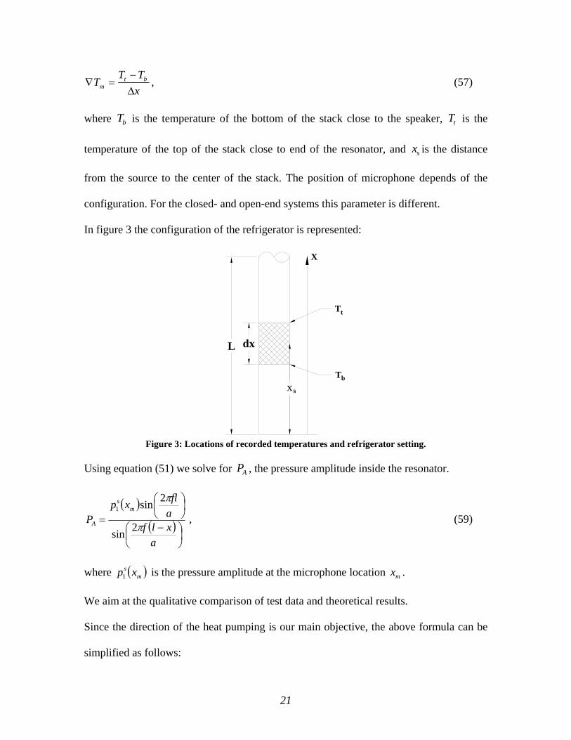
21
xTT
T btm Δ
−=∇ , (57)
where bT is the temperature of the bottom of the stack close to the speaker, tT is the
temperature of the top of the stack close to end of the resonator, and sx is the distance
from the source to the center of the stack. The position of microphone depends of the
configuration. For the closed- and open-end systems this parameter is different.
In figure 3 the configuration of the refrigerator is represented:
Figure 3: Locations of recorded temperatures and refrigerator setting.
Using equation (51) we solve for AP , the pressure amplitude inside the resonator.
( )
( )⎟⎠⎞
⎜⎝⎛ −
⎟⎠⎞
⎜⎝⎛
=
axlfaflxp
Pm
s
A π
π
2sin
2sin1
, (59)
where ( )ms xp1
is the pressure amplitude at the microphone location mx .
We aim at the qualitative comparison of test data and theoretical results.
Since the direction of the heat pumping is our main objective, the above formula can be
simplified as follows:
dx
X
L
T
T
t
b
sx

22
22 ~ hH , (60)
( ) ( )ss
ss xuxph 112 = . (61)
For a closed ended system spatial variations of acoustic pressure and velocity are:
( ) ( ) ( )⎟⎠⎞
⎜⎝⎛ −
⎟⎟⎟⎟
⎠
⎞
⎜⎜⎜⎜
⎝
⎛
⎟⎠⎞
⎜⎝⎛
=a
xlf
aflPaxp As ππ
ρ 2cos2sin
2
1 , (62)
( )( )
⎟⎟⎟⎟
⎠
⎞
⎜⎜⎜⎜
⎝
⎛
⎟⎠⎞
⎜⎝⎛
⎟⎠⎞
⎜⎝⎛ −
=
afl
axlf
aPxu As
π
π
ρ2sin
2sin1 , (63)
For estimating the thermoacoustic enthalpy flow, equations (60) and (61) can be used for
the closed-end system as well.
23
2.2. Experimental Setups
2.2.1. Heat Engine
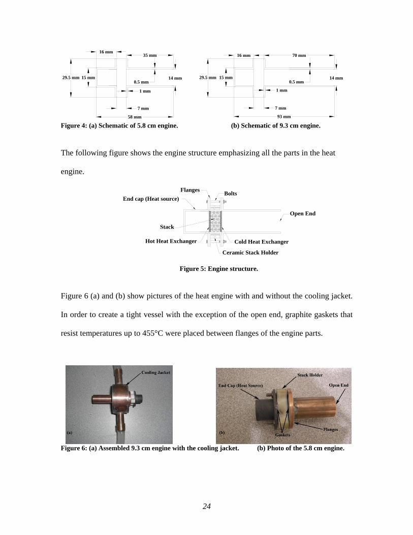
The resonator of the engine consists of three parts. The first part is the tube with
one end closed acting as the hot heat exchanger in the system. It is made of solid copper
tubing, which was machined down to appropriate dimensions. The second part is the
ceramic stack holder that contains a cavity with the same inner diameter as the copper
tube. The third part is the open-end tube made of copper and similarly machined to the
right dimensions. Flanges were added to each part, which were connected with each by
long screws tightened with nuts for the integrity of assembly. The heat exchangers were
two layers of thin copper mesh placed on each side of the stack. The assembled engine is
schematically shown in figure 5. The materials used for the stack were similar to the
Hofler tube [7]: Reticulated Vitreous Carbon foam (RVC) with two different densities
and a steel wool. RVC is a porous structure or open-celled foam consisting of an
interconnected network of solid fibers. RVCs can be specified with two different
characteristics: the number of pores per inch (PPI) and volumetric porosity [8]. The
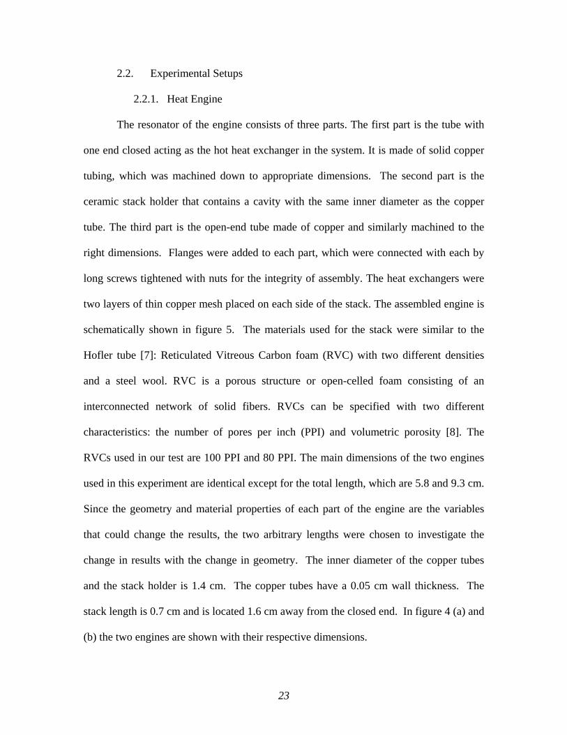
RVCs used in our test are 100 PPI and 80 PPI. The main dimensions of the two engines
used in this experiment are identical except for the total length, which are 5.8 and 9.3 cm.
Since the geometry and material properties of each part of the engine are the variables
that could change the results, the two arbitrary lengths were chosen to investigate the
change in results with the change in geometry. The inner diameter of the copper tubes
and the stack holder is 1.4 cm. The copper tubes have a 0.05 cm wall thickness. The
stack length is 0.7 cm and is located 1.6 cm away from the closed end. In figure 4 (a) and
(b) the two engines are shown with their respective dimensions.
24
Figure 4: (a) Schematic of 5.8 cm engine. (b) Schematic of 9.3 cm engine.
The following figure shows the engine structure emphasizing all the parts in the heat
engine.
Figure 5: Engine structure.
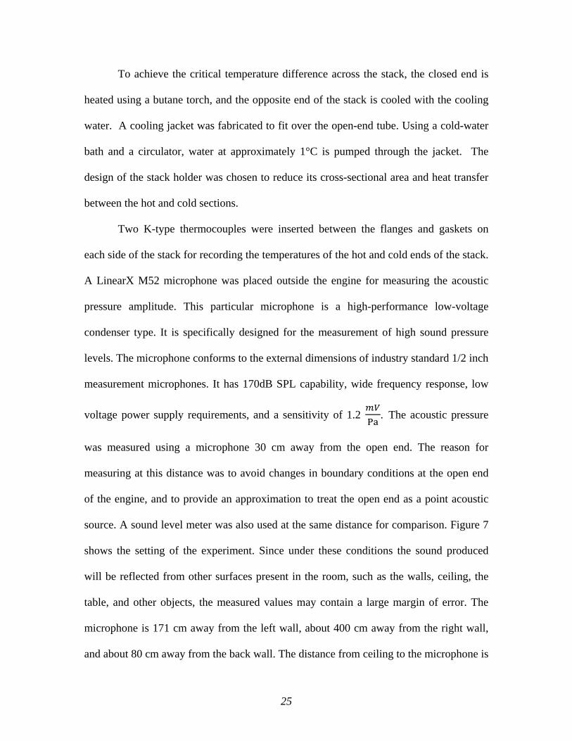
Figure 6 (a) and (b) show pictures of the heat engine with and without the cooling jacket.
In order to create a tight vessel with the exception of the open end, graphite gaskets that
resist temperatures up to 455°C were placed between flanges of the engine parts.
Figure 6: (a) Assembled 9.3 cm engine with the cooling jacket. (b) Photo of the 5.8 cm engine.
0.5 mm14 mm
7 mm
15 mm29.5 mm
58 mm
35 mm16 mm
1 mm
0.5 mm14 mm
7 mm
15 mm29.5 mm
93 mm
70 mm
1 mm
16 mm
End cap (Heat source)Flanges
Open End
Hot Heat Exchanger Cold Heat Exchanger
Stack
Bolts
Ceramic Stack Holder
25
To achieve the critical temperature difference across the stack, the closed end is
heated using a butane torch, and the opposite end of the stack is cooled with the cooling
water. A cooling jacket was fabricated to fit over the open-end tube. Using a cold-water
bath and a circulator, water at approximately 1°C is pumped through the jacket. The
design of the stack holder was chosen to reduce its cross-sectional area and heat transfer
between the hot and cold sections.
Two K-type thermocouples were inserted between the flanges and gaskets on
each side of the stack for recording the temperatures of the hot and cold ends of the stack.
A LinearX M52 microphone was placed outside the engine for measuring the acoustic
pressure amplitude. This particular microphone is a high-performance low-voltage
condenser type. It is specifically designed for the measurement of high sound pressure
levels. The microphone conforms to the external dimensions of industry standard 1/2 inch
measurement microphones. It has 170dB SPL capability, wide frequency response, low
voltage power supply requirements, and a sensitivity of 1.2 P
. The acoustic pressure
was measured using a microphone 30 cm away from the open end. The reason for
measuring at this distance was to avoid changes in boundary conditions at the open end
of the engine, and to provide an approximation to treat the open end as a point acoustic
source. A sound level meter was also used at the same distance for comparison. Figure 7
shows the setting of the experiment. Since under these conditions the sound produced
will be reflected from other surfaces present in the room, such as the walls, ceiling, the
table, and other objects, the measured values may contain a large margin of error. The
microphone is 171 cm away from the left wall, about 400 cm away from the right wall,
and about 80 cm away from the back wall. The distance from ceiling to the microphone is

26
about 15 m and from the microphone to the ground is about 130 cm. The distance to the
table is about 26 cm where soft foam was placed on for acoustic damping. Under these
specific conditions the acoustic pressure was measured.
Figure 7: Heat engine experimental setup.
2.2.2. Refrigerator
The refrigerator is driven by a 100 W RCA 4” 2-way full range speaker made by
Smart Mobile Technology. The speaker is mounted to a 5 cm thick plastic plate. This
plate has a hole with the size of the speaker to allow vertical movement of air. A 1 cm
thick plastic plate, with a hole in the center the same size as the resonator, is screwed to
the 5 cm plate, and an acrylic tube is inserted in the thinner plate. For the open end, the
resonator is 17.5 cm long with an internal diameter of 3 cm. In the case of the closed end,
the length of the tube is 29 cm so that a cap can be screwed on top, but the inner diameter
was machined to be the same. Figure 8 shows a representation of both systems with all
parts and main dimensions.

27
Figure 8: (a) Schematics of open-end system. (b) Schematic of closed-end system
For each configuration, different types of stacks were tested in order to find the
most efficient stack for each system. The stack materials included cotton wool, steel wool
with two different densities, and ceramics with two different porosities. The steel wool is
a bundle of strands of very fine soft steel filaments with a fiber diameter of 50 µm for
super-fine and 80 µm for fine wool. This particular steel wool is a production of Rhodes
American Steel Wool. The two grades that responded to our system were the super fine
and extra fine. The Celcor cellular ceramic substrates used in our experiment are made by
Corning Incorporated and they have been widely used at the core of the catalytic
converters. The ceramic substrates have high temperature durability and can effectively
operate at temperatures up to 1200 °C. Their single piece structure and cellular geometry
ensure stiffness and mechanical durability. The particular ceramic used in these
experiments has a porosity of 35% [20]. The ceramic structure is parallel plates that are
placed vertically, creating square shaped gaps. These squares have a side length of
approximately 1 mm. For our system the best results were obtained using the super-fine
290 mm
50 mm
10 mm
30 mm
sx
50 mm
175 mm
10 mm
30 mm
sx
135 mm
28
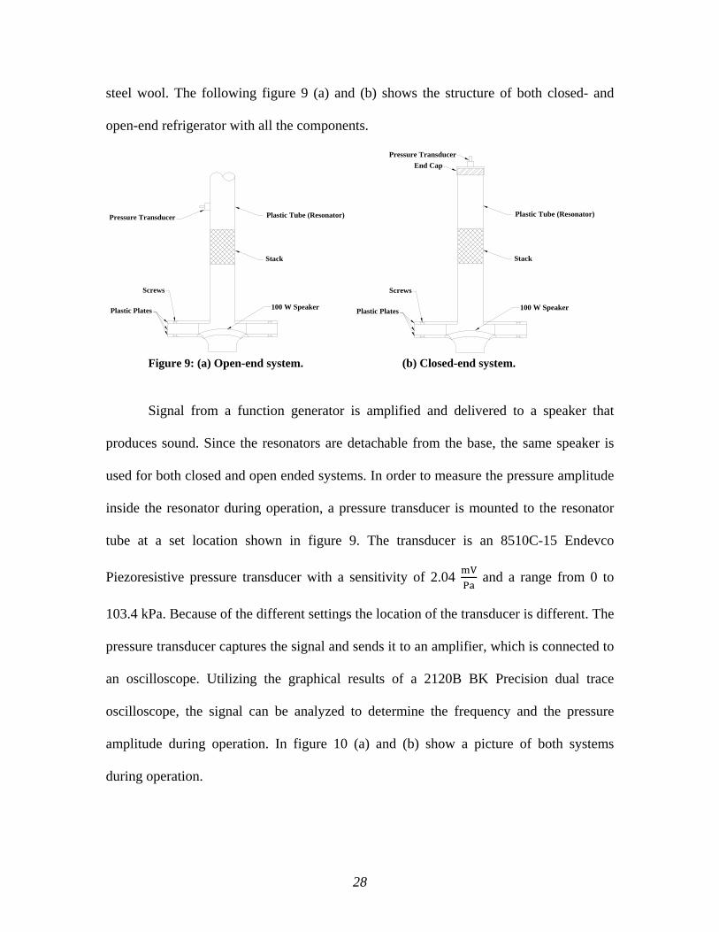
steel wool. The following figure 9 (a) and (b) shows the structure of both closed- and
open-end refrigerator with all the components.
Figure 9: (a) Open-end system. (b) Closed-end system.
Signal from a function generator is amplified and delivered to a speaker that
produces sound. Since the resonators are detachable from the base, the same speaker is
used for both closed and open ended systems. In order to measure the pressure amplitude
inside the resonator during operation, a pressure transducer is mounted to the resonator
tube at a set location shown in figure 9. The transducer is an 8510C-15 Endevco
Piezoresistive pressure transducer with a sensitivity of 2.04 VP
and a range from 0 to
103.4 kPa. Because of the different settings the location of the transducer is different. The
pressure transducer captures the signal and sends it to an amplifier, which is connected to
an oscilloscope. Utilizing the graphical results of a 2120B BK Precision dual trace
oscilloscope, the signal can be analyzed to determine the frequency and the pressure
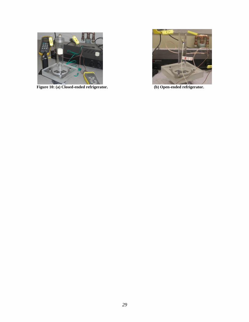
amplitude during operation. In figure 10 (a) and (b) show a picture of both systems
during operation.
Stack
Plastic Tube (Resonator)
100 W SpeakerPlastic Plates
Screws
Pressure Transducer
Stack
Plastic Tube (Resonator)
100 W SpeakerPlastic Plates
Screws
Pressure TransducerEnd Cap
29
Figure 10: (a) Closed-ended refrigerator. (b) Open-ended refrigerator.

30
Chapter 3
Results and Discussion
31
3. Results and Discussions
In this section all the experimental results for both heat engine and refrigerator are
presented, discussed and compared to theoretical results.
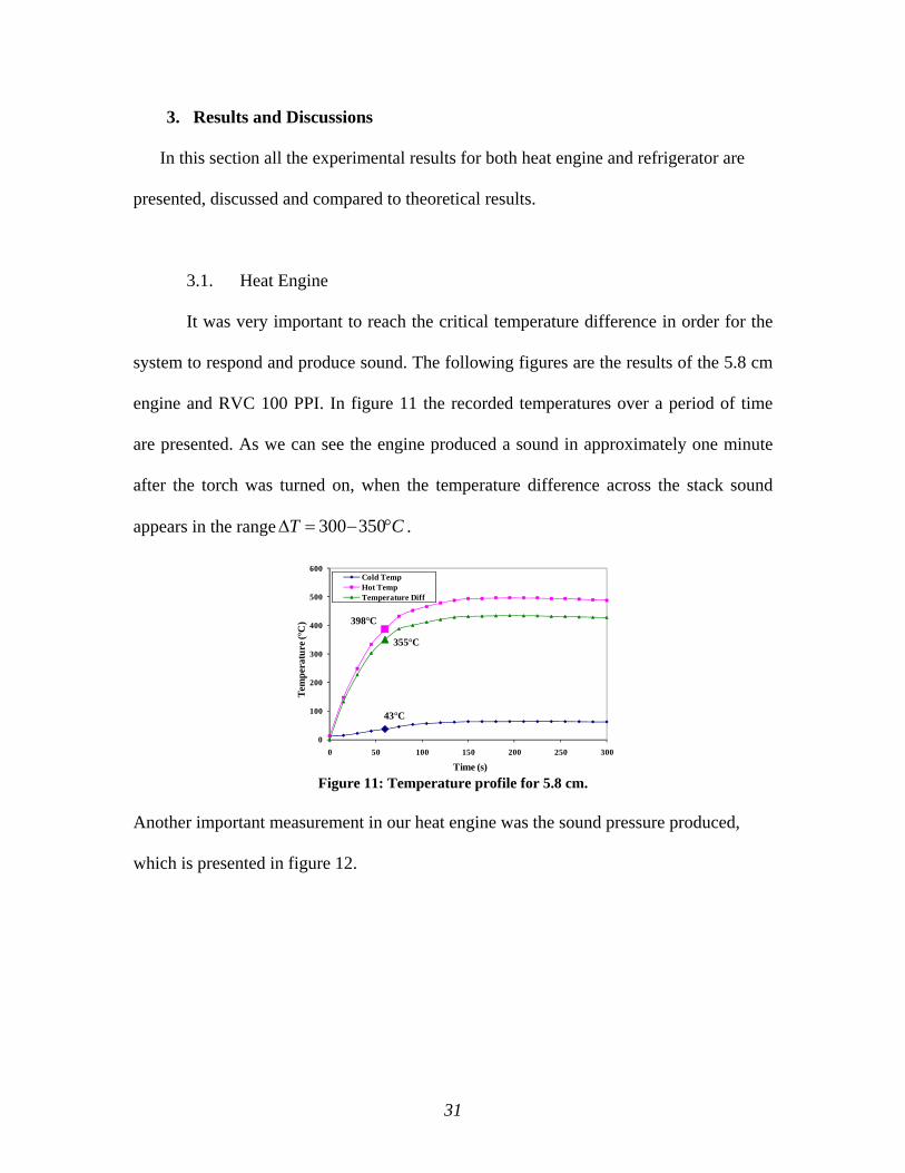
3.1. Heat Engine
It was very important to reach the critical temperature difference in order for the
system to respond and produce sound. The following figures are the results of the 5.8 cm
engine and RVC 100 PPI. In figure 11 the recorded temperatures over a period of time
are presented. As we can see the engine produced a sound in approximately one minute
after the torch was turned on, when the temperature difference across the stack sound
appears in the range CT °−=Δ 350300 .
Figure 11: Temperature profile for 5.8 cm.
Another important measurement in our heat engine was the sound pressure produced,
which is presented in figure 12.
43°C
398°C
355°C
0
100
200
300
400
500
600
0 50 100 150 200 250 300
Tem
pera
ture
(°C
)
Time (s)
Cold TempHot TempTemperature Diff
32
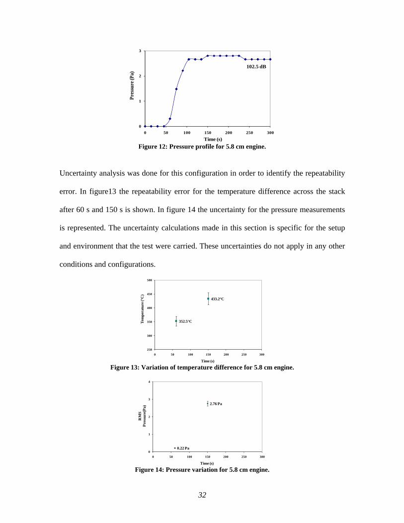
Figure 12: Pressure profile for 5.8 cm engine.
Uncertainty analysis was done for this configuration in order to identify the repeatability
error. In figure13 the repeatability error for the temperature difference across the stack
after 60 s and 150 s is shown. In figure 14 the uncertainty for the pressure measurements
is represented. The uncertainty calculations made in this section is specific for the setup
and environment that the test were carried. These uncertainties do not apply in any other
conditions and configurations.
Figure 13: Variation of temperature difference for 5.8 cm engine.
Figure 14: Pressure variation for 5.8 cm engine.
102.5 dB
0
1
2
3
0 50 100 150 200 250 300Pr
essu
re (P
a)Time (s)
352.5°C
433.2°C
250
300
350
400
450
500
0 50 100 150 200 250 300
Tem
pera
ture
(°C
)
Time (s)
0.22 Pa
2.76 Pa
0
1
2
3
4
0 50 100 150 200 250 300
RM
SPr
essu
re(P
a)
Time (s)

33
Table 1: Tabulated temperature uncertainty calculations.
Table 2: Tabulated pressure uncertainty calculations.
In figure 15 the pressure amplitude of the system is plotted against temperature
difference across the stack. Here we can see that after reaching certain temperature at the
hot end of the engine, in this case 500 °C, the system reaches steady state and the change
in pressure amplitude is not drastic. From the time the sound produced to the time the
sound reaches maximum amplitude is about 135 s. The recorded temperature of the heat
Time (s) 60 150T1 (°C) 350 433T2 (°C) 359 431T3 (°C) 343 443T4 (°C) 353 426T5 (°C) 366 431T6 (°C) 343 429T7 (°C) 350 428T8 (°C) 356 432T9 (°C) 348 440T10 (°C) 357 439
Avg. Temp. (°C) 352.50 433.20Linearity (°C) 0.7 0.7
Thermocouple Sensitivity (°C) 0.35 0.35Thermometer Sensitivity (°C) 2.06 2.30
Zero Shift (°C) 0.50 0.50Standard Dev. (°C) 7.23 5.61
Standard Dev. of Mean (°C) 2.29 1.78Total Bias (°C) 2.26 2.48
Total Uncertainty (°C) 5.10 4.33
Time (s) 60 150P1 (Pa) 0.2 2.8P2 (Pa) 0.1 2.8P3 (Pa) 0.3 2.8P4 (Pa) 0.3 2.65P5 (Pa) 0.3 2.8P6 (Pa) 0.2 2.65P7 (Pa) 0.1 2.8P8 (Pa) 0.2 2.8P9 (Pa) 0.1 2.65P10 (Pa) 0.4 2.8
Avg. Acoustic Pressure (Pa) 0.22 2.76Oscilloscope Readability error (Pa) 0.09 0.09
Microphone Sensitivity (Pa) 0.018 0.23Standard Dev. (Pa) 0.10 0.07
Standard Dev. of Mean (Pa) 0.03 0.02Total Bias (Pa) 0.09 0.25
Total Uncertainty (Pa) 0.23 0.25
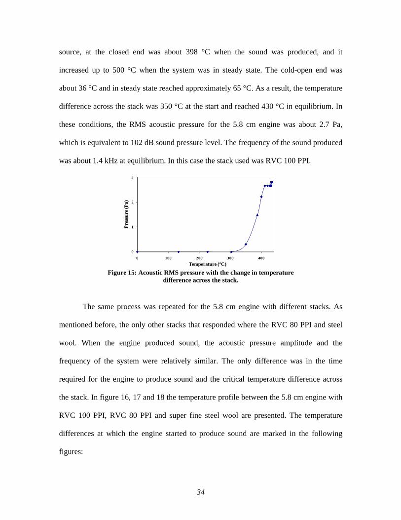
34
source, at the closed end was about 398 °C when the sound was produced, and it
increased up to 500 °C when the system was in steady state. The cold-open end was
about 36 °C and in steady state reached approximately 65 °C. As a result, the temperature
difference across the stack was 350 °C at the start and reached 430 °C in equilibrium. In
these conditions, the RMS acoustic pressure for the 5.8 cm engine was about 2.7 Pa,
which is equivalent to 102 dB sound pressure level. The frequency of the sound produced
was about 1.4 kHz at equilibrium. In this case the stack used was RVC 100 PPI.
Figure 15: Acoustic RMS pressure with the change in temperature
difference across the stack.
The same process was repeated for the 5.8 cm engine with different stacks. As
mentioned before, the only other stacks that responded where the RVC 80 PPI and steel
wool. When the engine produced sound, the acoustic pressure amplitude and the
frequency of the system were relatively similar. The only difference was in the time
required for the engine to produce sound and the critical temperature difference across
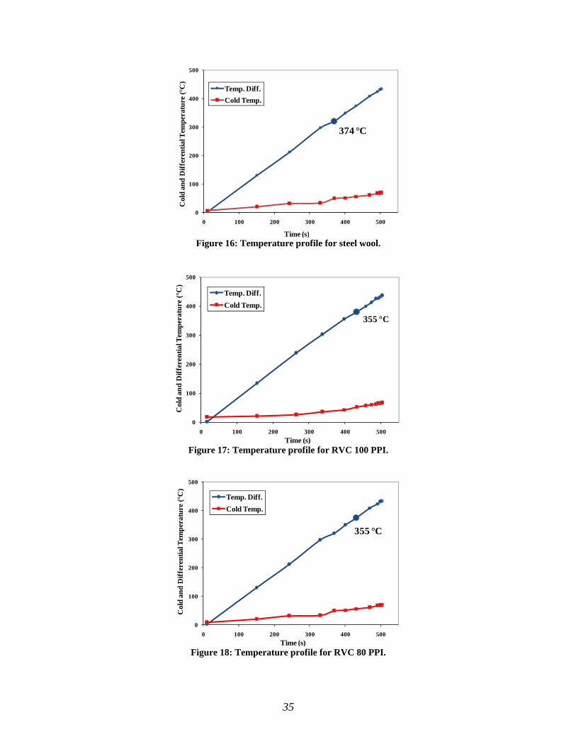
the stack. In figure 16, 17 and 18 the temperature profile between the 5.8 cm engine with
RVC 100 PPI, RVC 80 PPI and super fine steel wool are presented. The temperature
differences at which the engine started to produce sound are marked in the following
figures:
0
1
2
3
0 100 200 300 400
Pres
sure
(Pa)
Temperature (°C)
35
Figure 16: Temperature profile for steel wool.
Figure 17: Temperature profile for RVC 100 PPI.
Figure 18: Temperature profile for RVC 80 PPI.
374 °C
0
100
200
300
400
500
0 100 200 300 400 500
Col
d an
d D
iffer
entia
l Tem
pera
ture
(°C
)
Time (s)
Temp. Diff.Cold Temp.
355 °C
0
100
200
300
400
500
0 100 200 300 400 500
Col
d an
d D
iffer
entia
l Tem
pera
ture
(°C
)
Time (s)
Temp. Diff.Cold Temp.
355 °C
0
100
200
300
400
500
0 100 200 300 400 500
Col
d an
d D
iffer
entia
l Tem
pera
ture
(°C
)
Time (s)
Temp. Diff.Cold Temp.

36
The sound pressure level in all three cases reached a maximum of approximately
103 dB. In figure 19 the results for 5.8 cm engine with three different stack materials are
shown. In this case the temperature difference was recorded over 180 s time period. We
can see that the RVC PPI 100 and PPI 80 have very similar results. Both materials
require approximately 60 seconds and a temperature difference across the stack at about
350 °C in order to produce sound. In the case of steel wool the sound was produced after
about 90 seconds and a temperature difference of about 380 °C was required for the
engine to respond.
Figure 19: Temperature difference for RVC 100 PPI, 80 PPI, and steel-wool for 5.8 cm engine.
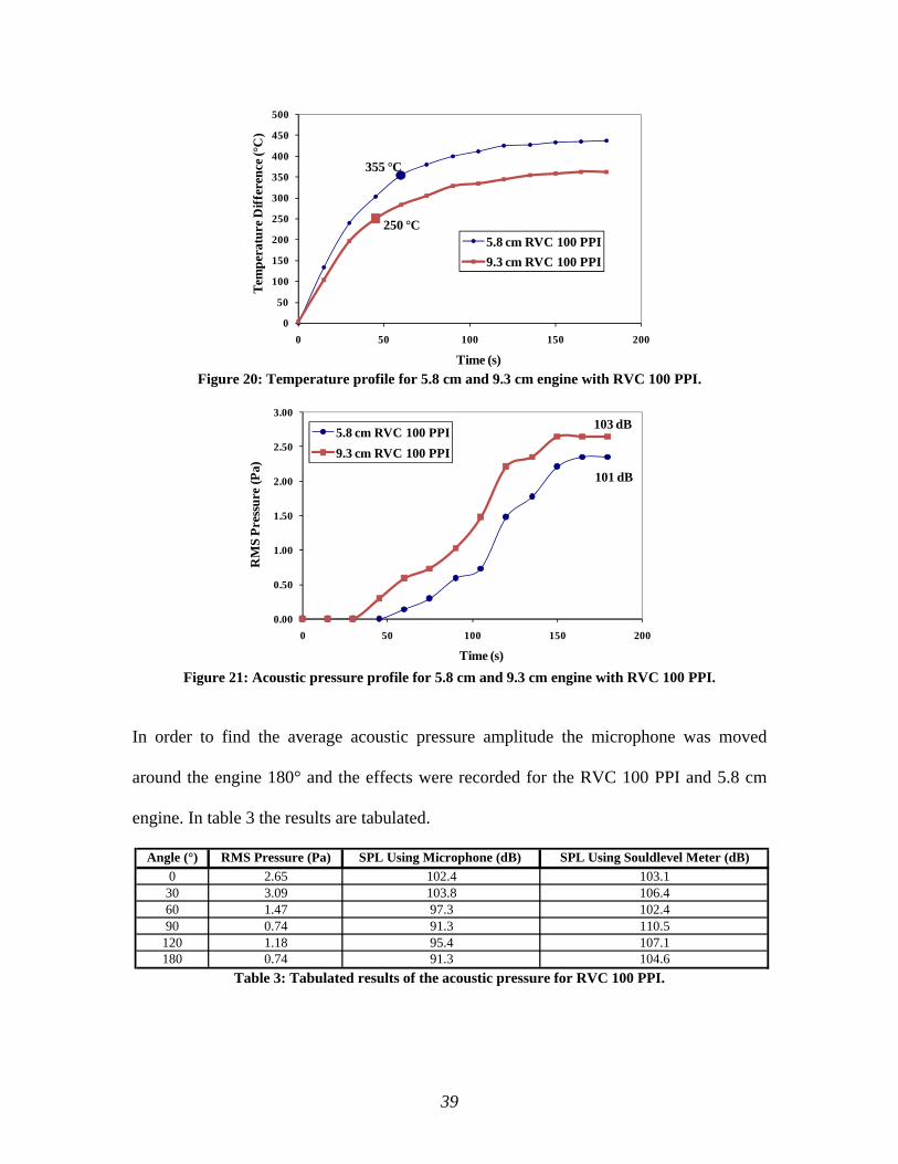
The following results represent the temperature difference and the pressure
distribution for RVC 100 PPI stack in the 5.8 cm and 9.3 cm engine. In figures 20 and 21,
the temperature difference across the stack and acoustic pressure distribution were plotted
over 180 second time period in order to see how long it takes for the engines to produce
sound and reach equilibrium. The results show that for the 5.8 cm engine we require
about 60 seconds in order to produce sound, but for the 9.3 cm engine, after only 45
second, sound was produced. Also, a lower temperature difference across the stack was
required for the longer engine to perform. The experimental results were compared to the
356 °C 374 °C
0
50
100
150
200
250
300
350
400
450
500
0 50 100 150 200
Tem
pera
ture
Diff
eren
ce (°
C)
Time (s)
RVC 100 PPIRVC 80 PPISteel Wool

37
theoretical analysis from section 2.1.1. The stack used in our system was an RVC with
non-uniform geometry, therefore the surface area needed to be recalculated. The RVC of
100 PPI and 80 PPI have 97% porosity. In order to calculate the surface area of the RVC
it was assumed that the stack is a solid material with uniform holes across it. This
assumption neglects the empty spaces between the holes and uses the porosity of the
RVC to determine the approximated perimeter. Making these assumptions the surface
area determined to be as follows:
rRxxS s
s
28.1 Δ=ΔΠ=
π . (64)
where R is the inner radius of the stack holder, r
is the radius of the small cylinders, and
sxΔ is the length of the stack.
Using the new surface area formula for the 5.8 cm engine, the required
temperature difference calculated is about 212 °C; and for the 9.3 cm it is about 173 °C.
However, the theoretical calculations contain idealized assumptions because of
irregularities in the stack geometry and the assumptions made to calculate the surface
area. Also, the theoretical results do not take into account the heat loss to the environment
and assume perfect conditions; therefore the theoretical results are significantly lower
than the measured values.
The pressure was calculated for different temperatures to compare with the
acoustic pressure measured 30 cm away from the open end. In order to calculate the
acoustic pressure we assume that the open end of the engine is a point source located in
the center of a sphere with a radius of 30 cm (the distance between the engine and the
microphone). We calculate the radiated energy from the point source to the sphere using
equation (24) from section 2.1.1. Since energy is conserved the radiated energy from
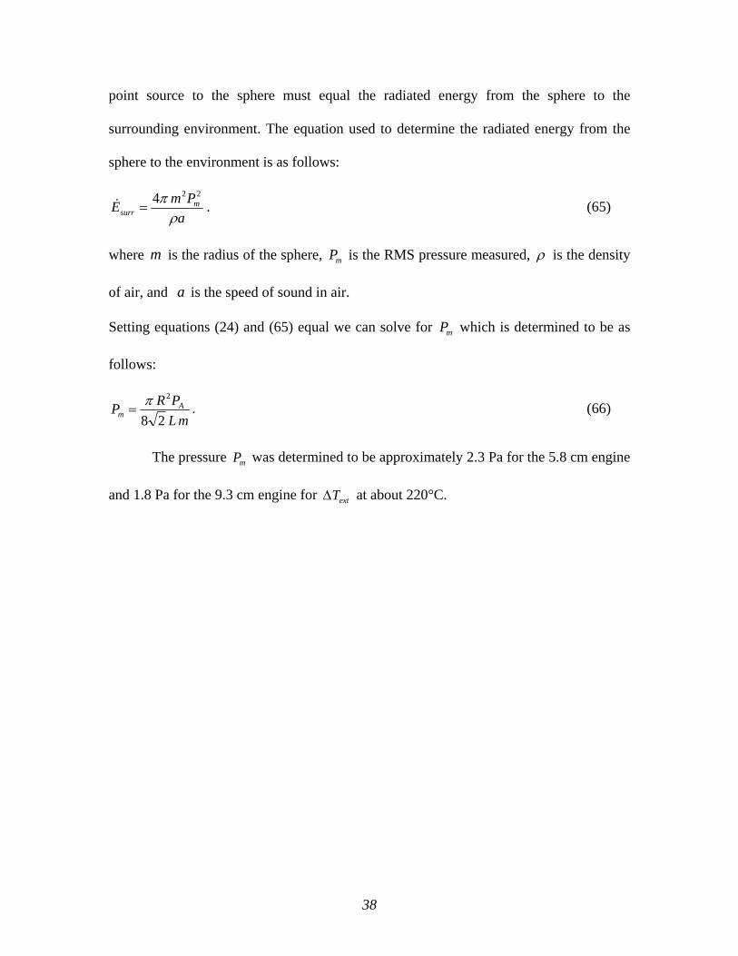
38
point source to the sphere must equal the radiated energy from the sphere to the
surrounding environment. The equation used to determine the radiated energy from the
sphere to the environment is as follows:
aPmE m
surr ρπ 224
=& . (65)
where m is the radius of the sphere, mP
is the RMS pressure measured, ρ
is the density
of air, and a is the speed of sound in air.
Setting equations (24) and (65) equal we can solve for mP which is determined to be as
follows:
mLPRP A
m 28
2π= . (66)
The pressure mP was determined to be approximately 2.3 Pa for the 5.8 cm engine
and 1.8 Pa for the 9.3 cm engine for extTΔ at about 220°C.
39
Figure 20: Temperature profile for 5.8 cm and 9.3 cm engine with RVC 100 PPI.
Figure 21: Acoustic pressure profile for 5.8 cm and 9.3 cm engine with RVC 100 PPI.
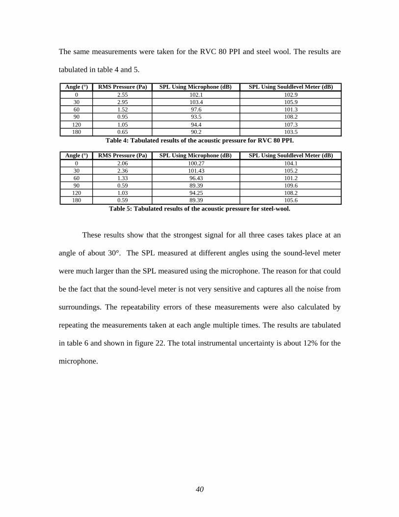
In order to find the average acoustic pressure amplitude the microphone was moved
around the engine 180° and the effects were recorded for the RVC 100 PPI and 5.8 cm
engine. In table 3 the results are tabulated.
Table 3: Tabulated results of the acoustic pressure for RVC 100 PPI.
355 °C
250 °C
0
50
100
150
200
250
300
350
400
450
500
0 50 100 150 200
Tem
pera
ture
Diff
eren
ce (°
C)
Time (s)
5.8 cm RVC 100 PPI9.3 cm RVC 100 PPI
101 dB
103 dB
0.00
0.50
1.00
1.50
2.00
2.50
3.00
0 50 100 150 200
RM
S Pr
essu
re (P
a)
Time (s)
5.8 cm RVC 100 PPI9.3 cm RVC 100 PPI
Angle (°) RMS Pressure (Pa) SPL Using Microphone (dB) SPL Using Souldlevel Meter (dB)0 2.65 102.4 103.1
30 3.09 103.8 106.460 1.47 97.3 102.490 0.74 91.3 110.5
120 1.18 95.4 107.1180 0.74 91.3 104.6
40
The same measurements were taken for the RVC 80 PPI and steel wool. The results are
tabulated in table 4 and 5.
Table 4: Tabulated results of the acoustic pressure for RVC 80 PPI.
Table 5: Tabulated results of the acoustic pressure for steel-wool.
These results show that the strongest signal for all three cases takes place at an
angle of about 30°. The SPL measured at different angles using the sound-level meter
were much larger than the SPL measured using the microphone. The reason for that could
be the fact that the sound-level meter is not very sensitive and captures all the noise from
surroundings. The repeatability errors of these measurements were also calculated by
repeating the measurements taken at each angle multiple times. The results are tabulated
in table 6 and shown in figure 22. The total instrumental uncertainty is about 12% for the
microphone.
Angle (°) RMS Pressure (Pa) SPL Using Microphone (dB) SPL Using Souldlevel Meter (dB)0 2.55 102.1 102.9
30 2.95 103.4 105.960 1.52 97.6 101.390 0.95 93.5 108.2
120 1.05 94.4 107.3180 0.65 90.2 103.5
Angle (°) RMS Pressure (Pa) SPL Using Microphone (dB) SPL Using Souldlevel Meter (dB)0 2.06 100.27 104.1
30 2.36 101.43 105.260 1.33 96.43 101.290 0.59 89.39 109.6
120 1.03 94.25 108.2180 0.59 89.39 105.6

41
Figure 22: Acoustic pressure error measurements at different angles for 5.8 cm engine.
Table 6: Pressure uncertainty calculations for 5.3 cm engine at different angles.
Even though the results are very close for all three stack materials, we can
conclude that for 5.8 cm engine the RVC 100 PPI was the most suitable stack, resulting
to the highest acoustic pressure amplitude at all angles. Using this assumption and
equation (65) the acoustic power W& can be determined, which was 0.01 W and 0.04 W
for the 5.8 cm and 9.3 cm engine respectively. Because of the uncertainties in the
pressure and dimension measurement errors the uncertainties of the calculated acoustic
0.22 Pa
2.76 Pa
5.31
7.86
0
2
4
6
8
10
0 50 100 150 200
RM
SPr
essu
re(P
a)
Angle (°)
Angle (°) 0 30 90 180P1 (Pa) 0.2 2.8 5.4 8P2 (Pa) 0.1 2.8 5.5 8.2P3 (Pa) 0.3 2.8 5.3 7.8P4 (Pa) 0.3 2.65 5 7.35P5 (Pa) 0.3 2.8 5.3 7.8P6 (Pa) 0.2 2.65 5.1 7.55P7 (Pa) 0.1 2.8 5.5 8.2P8 (Pa) 0.2 2.8 5.4 8
Avg. Acoustic Pressure (Pa) 0.21 2.76 5.31 7.86Oscilloscope Readability error (Pa) 0.09 0.09 0.09 0.09
Microphone Sensitivity (Pa) 0.02 0.23 0.44 0.66Standard Dev. (Pa) 0.22 0.18 0.48 0.80
Standard Dev. of Mean (Pa) 0.07 0.06 0.15 0.25Total Bias (Pa) 0.09 0.25 0.45 0.66
Total Uncertainty (Pa) 0.17 0.27 0.54 0.83
42
power for these particular configurations were about 14%. The acoustic pressure
measurements were obtained by averaging the pressure amplitude obtained for the same
engine conditions but different microphone positions.
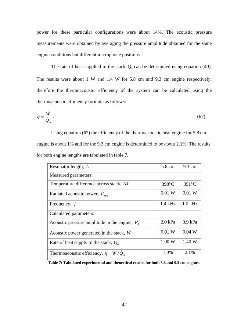
The rate of heat supplied to the stack inQ& can be determined using equation (40).
The results were about 1 W and 1.4 W for 5.8 cm and 9.3 cm engine respectively;
therefore the thermoacoustic efficiency of the system can be calculated using the
thermoacoustic efficiency formula as follows:
inQW&
&=η . (67)
Using equation (67) the efficiency of the thermoacoustic heat engine for 5.8 cm
engine is about 1% and for the 9.3 cm engine is determined to be about 2.1%. The results
for both engine lengths are tabulated in table 7.
Resonator length, L 5.8 cm 9.3 cm
Measured parameters:
Temperature difference across stack, TΔ 398°C 351°C
Radiated acoustic power, radE& 0.01 W 0.01 W
Frequency, f 1.4 kHz 1.0 kHz
Calculated parameters:
Acoustic pressure amplitude in the engine, AP 2.0 kPa 3.9 kPa
Acoustic power generated in the stack, W& 0.01 W 0.04 W
Rate of heat supply to the stack, inQ& 1.00 W 1.40 W
Thermoacoustic efficiency, inQW && /=η 1.0% 2.1%
Table 7: Tabulated experimental and theoretical results for both 5.8 and 9.3 cm engines.
43
3.2. Cooling Demonstrator
The main objective was to find the best stack location for each configuration and
measure the absolute value of the temperatures on both ends of the stack. The following
results are put together using different materials for the stack.
3.2.1. Closed-End System
In order to analyze the cooling demonstrator, the acoustic pressure inside the tube
and the frequency of the signal were varied, and for each case the temperature difference
across the stack was measured.
The closed system results show the system produces the highest temperature
difference across the stack as we move the stack closer to the closed end. It was also
observed that the sack side closer to the closed end of the tube was higher than the
opposite end of the stack. This conclusion was made by keeping the frequency and the
pressure amplitude of the signal the same during the operation, and moving the stack
along the resonator. The figures below show the development of temperature difference
as we move the stack in the resonator. In this case, ceramic with smaller holes were used.
The frequency of the signal input was also changed in order to find the optimum
frequency at which the system gives the best results. From previous experiments, it was
found that the optimum frequency was in vicinity of 220 Hz; the main frequency of 218
Hz was selected. In order to analyze the system for higher and lower frequencies, the
system was tested for frequencies both 100 Hz over and below the desired frequency.
44
This range was used because small changes in signal frequency did not change the results
significantly.
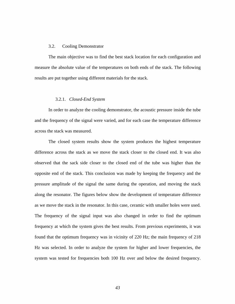
In figure 23, the temperature difference dependence of frequency is shown for the
stack at 13 cm. The stack was placed at 13 cm from the tube hole in the plate, the
frequency of the input signal was varied, and the temperature difference was recorded in
order to specify the best operating frequency for this system. These results conclude that
the optimum frequency in which the system operation is most efficient is between 200
and 230 Hz. Several frequencies between 200 and 230 Hz were tested. The speaker can
be used at 218 Hz over extended period of time without any damage.
Figure 23: Frequency profile for stack at 13 cm.
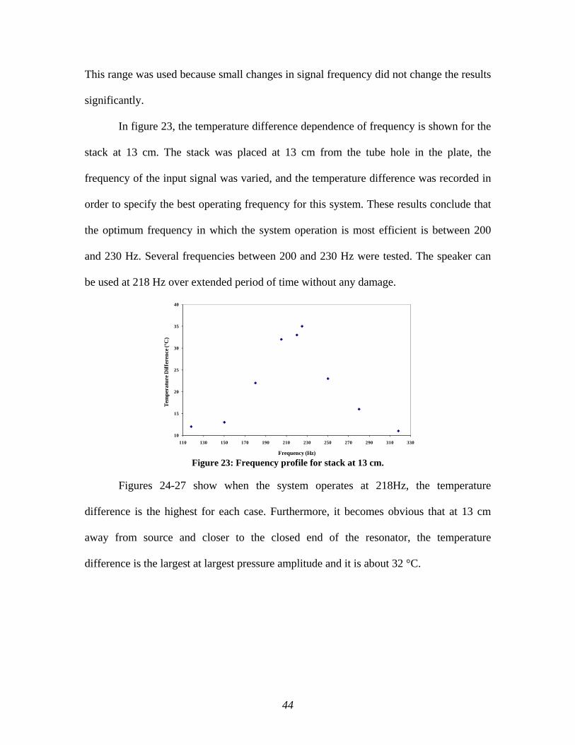
Figures 24-27 show when the system operates at 218Hz, the temperature
difference is the highest for each case. Furthermore, it becomes obvious that at 13 cm
away from source and closer to the closed end of the resonator, the temperature
difference is the largest at largest pressure amplitude and it is about 32 °C.
10
15
20
25
30
35
40
110 130 150 170 190 210 230 250 270 290 310 330
Tem
pera
ture
Diff
eren
ce (°
C)
Frequency (Hz)
45
Figure 24: Temperature difference for stack located at 7 cm.
Figure 25: Temperature difference for stack located at 9 cm.
Figure 26: Temperature difference for stack located at 11 cm.
5
10
15
20
0 1 2 3 4
Tem
p D
iffer
ence
(°C
)
RMS Pressure (kPa)
218 Hz118 Hz318 Hz
5
10
15
20
25
30
0 2 4
Tem
p D
iffer
ence
(°C
)
RMS Pressure (kPa)
218 Hz118 Hz318 Hz
0
5
10
15
20
25
30
0 1 2 3 4
Tem
p D
iffer
ence
(°C
)
RMS Pressure (kPa)
218 Hz118 Hz318 Hz
46
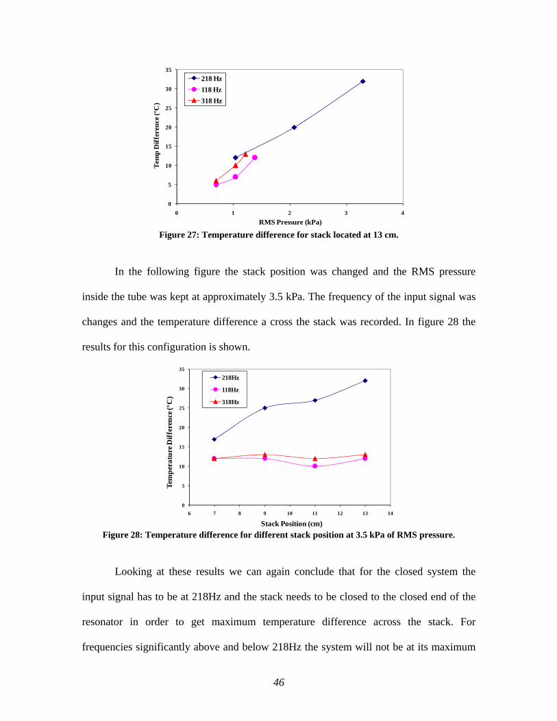
Figure 27: Temperature difference for stack located at 13 cm.
In the following figure the stack position was changed and the RMS pressure
inside the tube was kept at approximately 3.5 kPa. The frequency of the input signal was
changes and the temperature difference a cross the stack was recorded. In figure 28 the
results for this configuration is shown.
Figure 28: Temperature difference for different stack position at 3.5 kPa of RMS pressure.
Looking at these results we can again conclude that for the closed system the
input signal has to be at 218Hz and the stack needs to be closed to the closed end of the
resonator in order to get maximum temperature difference across the stack. For
frequencies significantly above and below 218Hz the system will not be at its maximum
0
5
10
15
20
25
30
35
0 1 2 3 4
Tem
p D
iffer
ence
(°C
)
RMS Pressure (kPa)
218 Hz118 Hz318 Hz
0
5
10
15
20
25
30
35
6 7 8 9 10 11 12 13 14
Tem
pera
ture
Diff
eren
ce (°
C)
Stack Position (cm)
218Hz
118Hz
318Hz
47
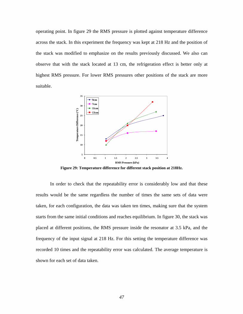
operating point. In figure 29 the RMS pressure is plotted against temperature difference
across the stack. In this experiment the frequency was kept at 218 Hz and the position of
the stack was modified to emphasize on the results previously discussed. We also can
observe that with the stack located at 13 cm, the refrigeration effect is better only at
highest RMS pressure. For lower RMS pressures other positions of the stack are more
suitable.
Figure 29: Temperature difference for different stack position at 218Hz.
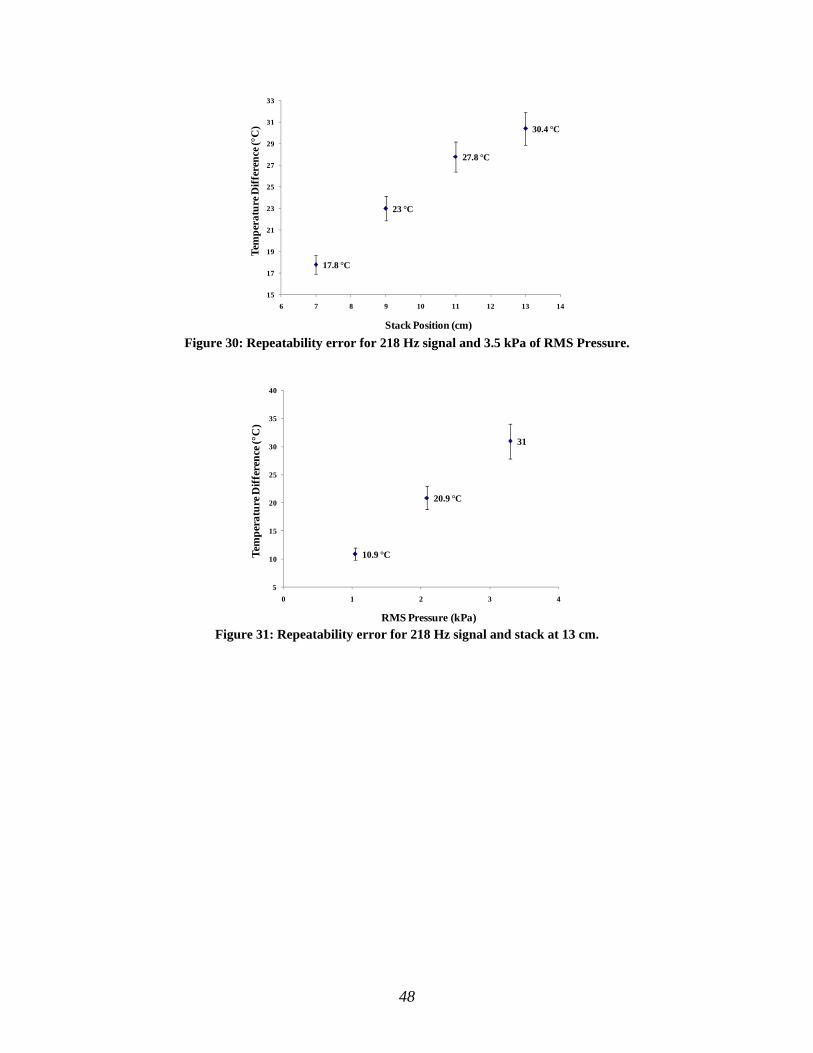
In order to check that the repeatability error is considerably low and that these
results would be the same regardless the number of times the same sets of data were
taken, for each configuration, the data was taken ten times, making sure that the system
starts from the same initial conditions and reaches equilibrium. In figure 30, the stack was
placed at different positions, the RMS pressure inside the resonator at 3.5 kPa, and the
frequency of the input signal at 218 Hz. For this setting the temperature difference was
recorded 10 times and the repeatability error was calculated. The average temperature is
shown for each set of data taken.
5
10
15
20
25
30
35
0 0.5 1 1.5 2 2.5 3 3.5 4
Tem
pera
ture
Diff
eren
ce (°
C)
RMS Pressure (kPa)
9cm7cm11cm13cm
48
Figure 30: Repeatability error for 218 Hz signal and 3.5 kPa of RMS Pressure.
Figure 31: Repeatability error for 218 Hz signal and stack at 13 cm.
17.8 °C
23 °C
27.8 °C
30.4 °C
15
17
19
21
23
25
27
29
31
33
6 7 8 9 10 11 12 13 14
Tem
pera
ture
Diff
eren
ce (°
C)
Stack Position (cm)
10.9 °C
20.9 °C
31
5
10
15
20
25
30
35
40
0 1 2 3 4
Tem
pera
ture
Diff
eren
ce (°
C)
RMS Pressure (kPa)
49
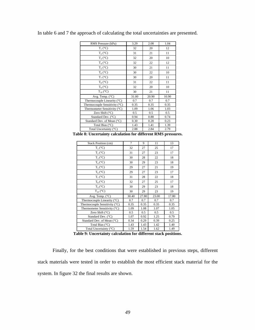
In table 6 and 7 the approach of calculating the total uncertainties are presented.
Table 8: Uncertainty calculation for different RMS pressures.
Table 9: Uncertainty calculation for different stack positions.
Finally, for the best conditions that were established in previous steps, different
stack materials were tested in order to establish the most efficient stack material for the
system. In figure 32 the final results are shown.
RMS Pressure (kPa) 3.29 2.08 1.04T1 (°C) 32 20 12T2 (°C) 31 21 11T3 (°C) 32 20 10T4 (°C) 32 22 12T5 (°C) 30 21 11T6 (°C) 30 22 10T7 (°C) 30 20 11T8 (°C) 31 22 11T9 (°C) 32 20 10T10 (°C) 30 21 11
Avg. Temp. (°C) 31.00 20.90 10.90Thermocouple Linearity (°C) 0.7 0.7 0.7
Thermocouple Sensitivity (°C) 0.35 0.35 0.35Thermometer Sensitivity (°C) 1.09 1.06 1.03
Zero Shift (°C) 0.5 0.5 0.5Standard Dev. (°C) 0.94 0.88 0.74
Standard Dev. of Mean (°C) 0.30 0.28 0.23Total Bias (°C) 1.43 1.41 1.39
Total Uncertainty (°C) 2.88 2.84 2.79
Stack Position (cm) 7 9 11 13T1 (°C) 32 27 25 17T2 (°C) 31 27 23 17T3 (°C) 30 28 22 18T4 (°C) 30 29 23 18T5 (°C) 29 27 21 19T6 (°C) 29 27 23 17T7 (°C) 31 28 22 18T8 (°C) 32 27 25 17T9 (°C) 30 29 23 18T10 (°C) 30 29 23 19
Avg. Temp. (°C) 30.40 27.80 23.00 17.80Thermocouple Linearity (°C) 0.7 0.7 0.7 0.7
Thermocouple Sensitivity (°C) 0.35 0.35 0.35 0.35Thermometer Sensitivity (°C) 1.09 1.08 1.07 1.05
Zero Shift (°C) 0.5 0.5 0.5 0.5Standard Dev. (°C) 1.07 0.92 1.25 0.79
Standard Dev. of Mean (°C) 0.34 0.29 0.39 0.25Total Bias (°C) 1.43 1.43 1.42 1.40
Total Uncertainty (°C) 1.59 1.54 1.62 1.49
50
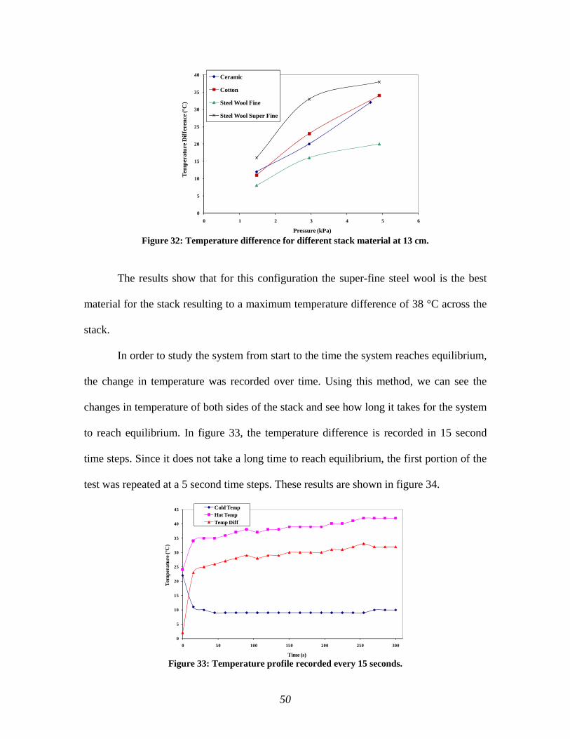
Figure 32: Temperature difference for different stack material at 13 cm.
The results show that for this configuration the super-fine steel wool is the best
material for the stack resulting to a maximum temperature difference of 38 °C across the
stack.
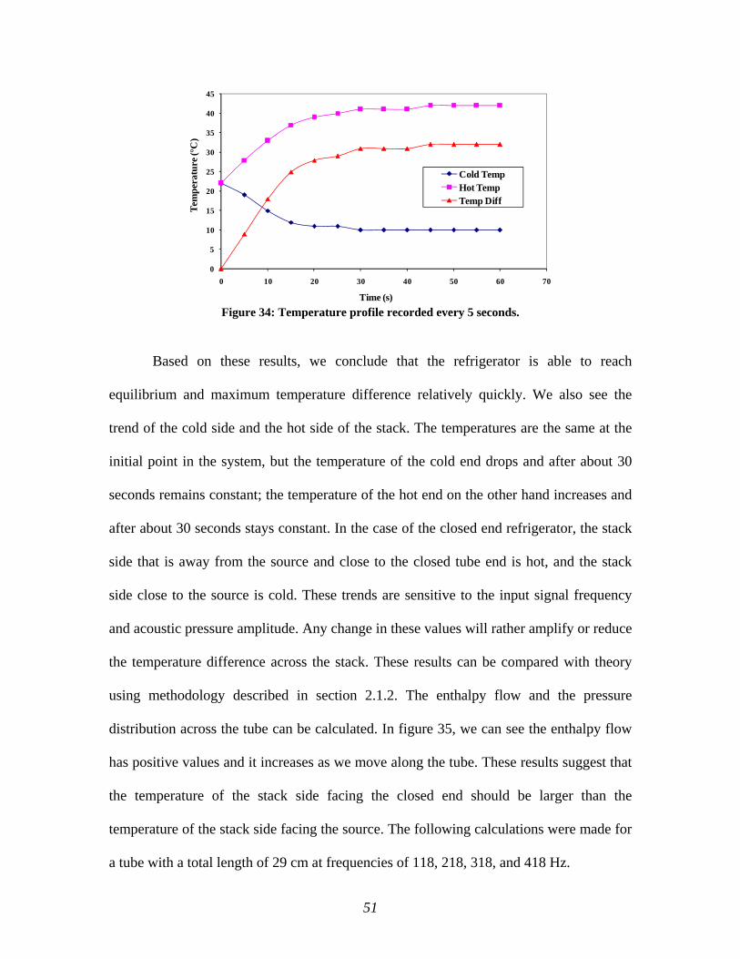
In order to study the system from start to the time the system reaches equilibrium,
the change in temperature was recorded over time. Using this method, we can see the
changes in temperature of both sides of the stack and see how long it takes for the system
to reach equilibrium. In figure 33, the temperature difference is recorded in 15 second
time steps. Since it does not take a long time to reach equilibrium, the first portion of the
test was repeated at a 5 second time steps. These results are shown in figure 34.
Figure 33: Temperature profile recorded every 15 seconds.
0
5
10
15
20
25
30
35
40
0 1 2 3 4 5 6
Tem
pera
ture
Diff
eren
ce (°
C)
Pressure (kPa)
Ceramic
Cotton
Steel Wool Fine
Steel Wool Super Fine
0
5
10
15
20
25
30
35
40
45
0 50 100 150 200 250 300
Tem
pera
ture
(°C
)
Time (s)
Cold TempHot TempTemp Diff
51
Figure 34: Temperature profile recorded every 5 seconds.
Based on these results, we conclude that the refrigerator is able to reach
equilibrium and maximum temperature difference relatively quickly. We also see the
trend of the cold side and the hot side of the stack. The temperatures are the same at the
initial point in the system, but the temperature of the cold end drops and after about 30
seconds remains constant; the temperature of the hot end on the other hand increases and
after about 30 seconds stays constant. In the case of the closed end refrigerator, the stack
side that is away from the source and close to the closed tube end is hot, and the stack
side close to the source is cold. These trends are sensitive to the input signal frequency
and acoustic pressure amplitude. Any change in these values will rather amplify or reduce
the temperature difference across the stack. These results can be compared with theory
using methodology described in section 2.1.2. The enthalpy flow and the pressure
distribution across the tube can be calculated. In figure 35, we can see the enthalpy flow
has positive values and it increases as we move along the tube. These results suggest that
the temperature of the stack side facing the closed end should be larger than the
temperature of the stack side facing the source. The following calculations were made for
a tube with a total length of 29 cm at frequencies of 118, 218, 318, and 418 Hz.
0
5
10
15
20
25
30
35
40
45
0 10 20 30 40 50 60 70
Tem
pera
ture
(°C
)
Time (s)
Cold TempHot TempTemp Diff

52
Figure 35: Enthalpy flow across the tube for a close-ended system.
3.2.2. Open System
The same approach was taken for the open-end system as for the closed-end
system. In the case of the open system, the stack needs to be closer to the sound source
for better performance. At this point, all the experiments are done using the steel wool as
the stack material, since the steel wool found to be the best choice for these
configurations. The temperature difference across the stack is much lower in the case of
open-end and the measured temperature close to the source is lower than the temperature
of the stack side close to the open end. Therefore the temperature difference across the
stack will be defined by subtracting the top temperature from the bottom temperature.
The following figures show the results for different stack position and different
frequencies. Because of the pressure transducer location, in open-end configuration, the
displacement range of the stack is small.
53
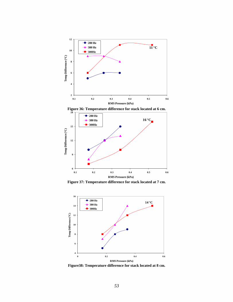
Figure 36: Temperature difference for stack located at 6 cm.
Figure 37: Temperature difference for stack located at 7 cm.
Figure38: Temperature difference for stack located at 8 cm.
11 °C
2
4
6
8
10
12
0.1 0.2 0.3 0.4 0.5 0.6
Tem
p D
iffer
ence
(°C
)
RMS Pressure (kPa)
280 Hz380 Hz300Hz
16 °C
6
9
12
15
18
0.1 0.2 0.3 0.4 0.5 0.6
Tem
p D
iffer
ence
(°C
)
RMS Pressure (kPa)
280 Hz380 Hz300Hz
14 °C
4
6
8
10
12
14
16
0 0.2 0.4 0.6
Tem
p D
iffer
ence
(°C
)
RMS Pressure (kPa)
280 Hz380 Hz300Hz
54
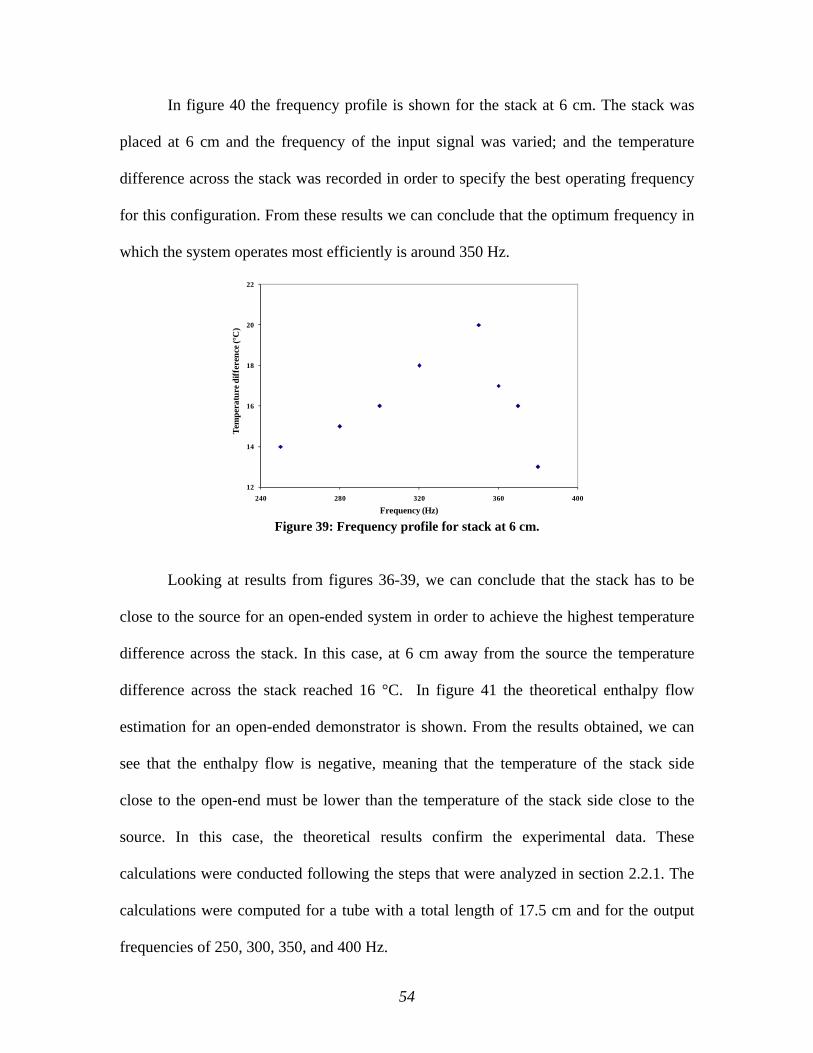
In figure 40 the frequency profile is shown for the stack at 6 cm. The stack was
placed at 6 cm and the frequency of the input signal was varied; and the temperature
difference across the stack was recorded in order to specify the best operating frequency
for this configuration. From these results we can conclude that the optimum frequency in
which the system operates most efficiently is around 350 Hz.
Figure 39: Frequency profile for stack at 6 cm.
Looking at results from figures 36-39, we can conclude that the stack has to be
close to the source for an open-ended system in order to achieve the highest temperature
difference across the stack. In this case, at 6 cm away from the source the temperature
difference across the stack reached 16 °C. In figure 41 the theoretical enthalpy flow
estimation for an open-ended demonstrator is shown. From the results obtained, we can
see that the enthalpy flow is negative, meaning that the temperature of the stack side
close to the open-end must be lower than the temperature of the stack side close to the
source. In this case, the theoretical results confirm the experimental data. These
calculations were conducted following the steps that were analyzed in section 2.2.1. The
calculations were computed for a tube with a total length of 17.5 cm and for the output
frequencies of 250, 300, 350, and 400 Hz.
12
14
16
18
20
22
240 280 320 360 400
Tem
pera
ture
diff
eren
ce (°
C)
Frequency (Hz)
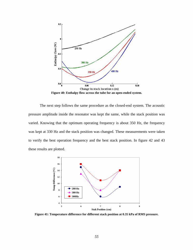
55
Figure 40: Enthalpy flow across the tube for an open-ended system.
The next step follows the same procedure as the closed-end system. The acoustic
pressure amplitude inside the resonator was kept the same, while the stack position was
varied. Knowing that the optimum operating frequency is about 350 Hz, the frequency
was kept at 330 Hz and the stack position was changed. These measurements were taken
to verify the best operation frequency and the best stack position. In figure 42 and 43
these results are plotted.
Figure 41: Temperature difference for different stack position at 0.35 kPa of RMS pressure.
4
6
8
10
12
14
16
18
5 6 7 8 9
Tem
p D
iffer
ence
(°C
)
Stak Position (cm)
280 Hz380 Hz300Hz
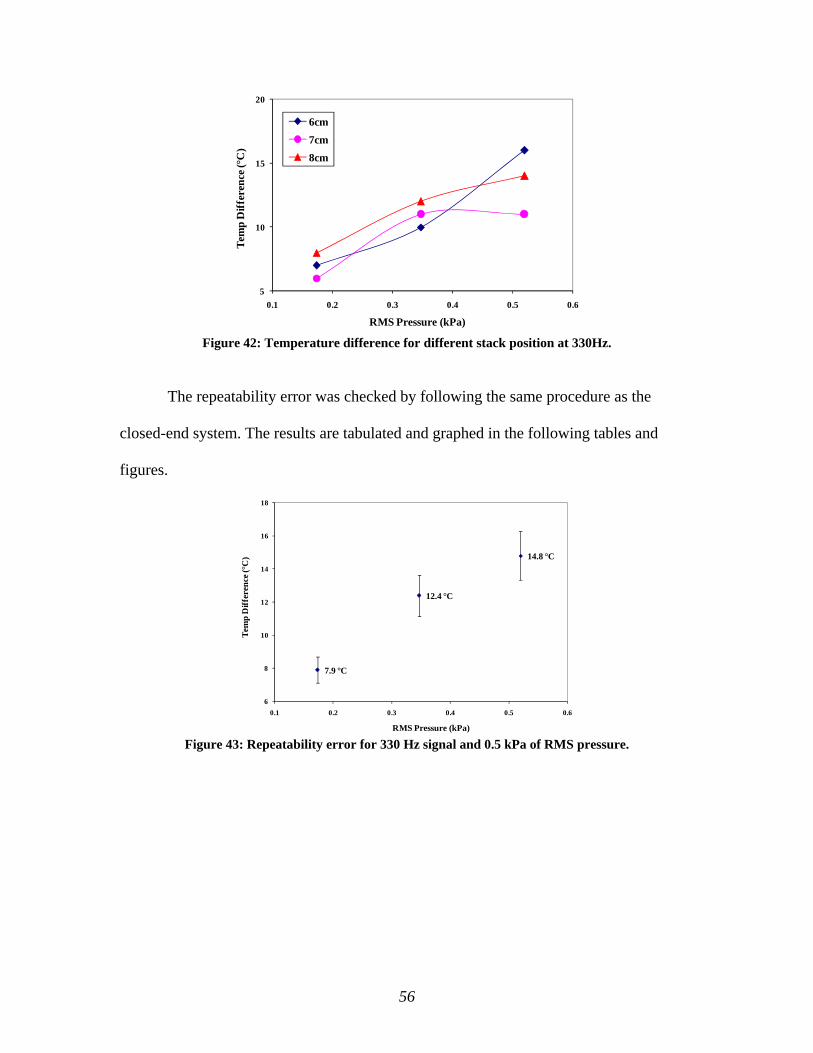
56
Figure 42: Temperature difference for different stack position at 330Hz.
The repeatability error was checked by following the same procedure as the
closed-end system. The results are tabulated and graphed in the following tables and
figures.
Figure 43: Repeatability error for 330 Hz signal and 0.5 kPa of RMS pressure.
5
10
15
20
0.1 0.2 0.3 0.4 0.5 0.6
Tem
p D
iffer
ence
(°C
)
RMS Pressure (kPa)
6cm7cm8cm
14.8 °C
12.4 °C
7.9 °C
6
8
10
12
14
16
18
0.1 0.2 0.3 0.4 0.5 0.6
Tem
p D
iffer
ence
(°C
)
RMS Pressure (kPa)

57
Table 10: Uncertainty calculation for different stack positions.
Figure 44: Repeatability error for 330 Hz signal and stack at 6 cm.
Stack Position (cm) 6 7 8
T1 (°C) 14 10 11T2 (°C) 15 10 11T3 (°C) 15 11 12T4 (°C) 16 11 12T5 (°C) 16 11 13T6 (°C) 16 11 13T7 (°C) 17 12 13T8 (°C) 15 11 12T9 (°C) 15 11 12T10 (°C) 16 11 13
Avg. Temp. (°C) 15.50 10.90 12.20Thermocouple Linearity (°C) 0.7 0.7 0.7
Thermocouple Sensitivity (°C) 0.35 0.35 0.35Thermometer Sensitivity (°C) 1.05 1.03 1.04
Zero Shift (°C) 0.5 0.5 0.5Standard Dev. (°C) 0.85 0.57 0.79
Standard Dev. of Mean (°C) 0.27 0.18 0.25Total Bias (°C) 1.40 1.39 1.39
Total Uncertainty (°C) 1.50 1.43 1.48
15.5 °C
10.9 °C
12.2 °C
8
10
12
14
16
18
5 6 7 8 9
Tem
p D
iffer
ence
(°C
)
Stak Position (cm)
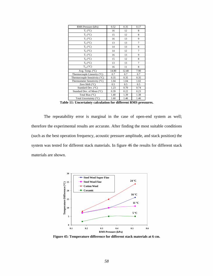
58
Table 11: Uncertainty calculation for different RMS pressures.
The repeatability error is marginal in the case of open-end system as well;
therefore the experimental results are accurate. After finding the most suitable conditions
(such as the best operation frequency, acoustic pressure amplitude, and stack position) the
system was tested for different stack materials. In figure 46 the results for different stack
materials are shown.
Figure 45: Temperature difference for different stack materials at 6 cm.
RMS Pressure (kPa) 0.52 0.35 0.17T1 (°C) 16 12 8T2 (°C) 15 12 8T3 (°C) 16 13 9T4 (°C) 13 13 7T5 (°C) 14 13 8T6 (°C) 14 12 7T7 (°C) 16 13 9T8 (°C) 15 12 8T9 (°C) 13 13 7T10 (°C) 16 11 8
Avg. Temp. (°C) 14.80 12.40 7.90Thermocouple Linearity (°C) 0.7 0.7 0.7
Thermocouple Sensitivity (°C) 0.35 0.35 0.35Thermometer Sensitivity (°C) 1.04 1.04 1.02
Zero Shift (°C) 0.5 0.5 0.5Standard Dev. (°C) 1.23 0.70 0.74
Standard Dev. of Mean (°C) 0.39 0.22 0.23Total Bias (°C) 1.40 1.39 1.38
Total Uncertainty (°C) 1.60 1.46 1.46
16 °C
11 °C
24 °C
5 °C
0
5
10
15
20
25
30
0.1 0.2 0.3 0.4 0.5 0.6
Tem
pera
ture
Diff
eren
ce (°
C)
RMS Pressure (kPa)
Steel Wool Super FineSteel Wool FineCotton WoolCeramic
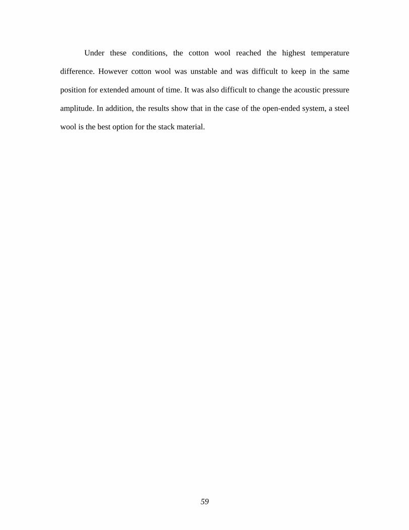
59
Under these conditions, the cotton wool reached the highest temperature
difference. However cotton wool was unstable and was difficult to keep in the same
position for extended amount of time. It was also difficult to change the acoustic pressure
amplitude. In addition, the results show that in the case of the open-ended system, a steel
wool is the best option for the stack material.

60
Chapter 4
Conclusion and Recommendations
61
4. Conclusions and Recommendations
In this study a thermoacoustic heat engine was successfully built and tested for
different conditions. During the tests, different stack materials and engine lengths were
used. The temperature difference across the stack and the acoustic pressure amplitude
were measured and compared with theoretical values.
The acoustic power radiated by the 5.8 cm long engine, with 100 PPI RVC as the
stack, is about 0.01 W, with a sound pressure level of approximately 106 dB measured 30
cm away from the open end of the engine. There are many variables that contribute to
exergy loss and performance reduction in the system. One possible way to increase the
performance of the heat engine will be to minimize the heat losses to the surrounding
medium. An important factor in the engine construction is the sealing between its parts.
The engine did not produce any sound before the gaskets were introduced between the
flanges of the system components. Presently, a flame is applied as a heat source in our
system; in the future the flame can be replaced with other more efficient heat sources. By
implementing a piezoelectric pressure transducer at the open end of the engine, the
acoustic power can be converted to electric power. Hence, the thermoacoustic heat engine
can be used as a small scale power source.
The microphone was placed outside the engine to measure the pressure amplitude
in the external acoustic field. In order to eliminate acoustic reflection uncertainty, the
system can be placed in an anechoic chamber that would minimize these reflections. The
acoustic power inside the engine is of main importance; therefore, a small cavity can be
added to the engine structure, where a pressure transducer can be inserted. In the future,
62
temperature and pressure data can be taken using a data acquisition system for better time
resolved measurements.
A cooling demonstrator was also built in this study. It was tested in different
conditions, open- and closed-end configurations. The results gave us an idea about the
most favorable stack material and location in each system. In both open and closed-end
systems, super fine steel wool was determined to be the best material used for stack.
In the closed system the stack has to be close to the closed end away from the
source to produce higher temperature difference across the stack. The temperature of the
stack side close to the cap was higher than the temperature of the stack side closer to the
source. In the case of the open system the effects were reversed; the closer the stack was
to the source and away from the open end, the higher the temperature difference across
the stack was observed. We can see that by changing the tube boundary conditions the
cooling effect can be influenced. It can be recommended to test other materials for the
stack, which can result in higher temperature differences across the stack. Since the
temperatures were taken using thermocouples connected to thermometers, recording the
change of temperature over time at a fast rate was difficult. The temperatures can be
recorded using a data acquisition system for better time resolution. The pressure
amplitude inside the resonator was monitored by a pressure transducer that was
connected to an oscilloscope. In the future, this pressure transducer can be also connected
to a data acquisition system for automatic readings. In order to use the full range of our
amplifier and maximize the heat pumping in the cooling demonstrator, more powerful
speakers can be implemented in the system.
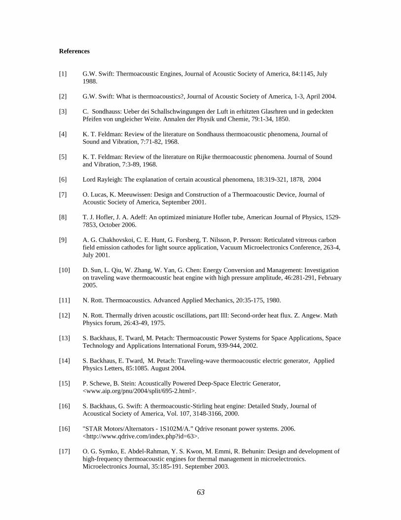
63
References
[1] G.W. Swift: Thermoacoustic Engines, Journal of Acoustic Society of America, 84:1145, July
1988. [2] G.W. Swift: What is thermoacoustics?, Journal of Acoustic Society of America, 1-3, April 2004. [3] C. Sondhauss: Ueber dei Schallschwingungen der Luft in erhitzten Glasrhren und in gedeckten
Pfeifen von ungleicher Weite. Annalen der Physik und Chemie, 79:1-34, 1850. [4] K. T. Feldman: Review of the literature on Sondhauss thermoacoustic phenomena, Journal of
Sound and Vibration, 7:71-82, 1968. [5] K. T. Feldman: Review of the literature on Rijke thermoacoustic phenomena. Journal of Sound
and Vibration, 7:3-89, 1968. [6] Lord Rayleigh: The explanation of certain acoustical phenomena, 18:319-321, 1878, 2004 [7] O. Lucas, K. Meeuwissen: Design and Construction of a Thermoacoustic Device, Journal of
Acoustic Society of America, September 2001. [8] T. J. Hofler, J. A. Adeff: An optimized miniature Hofler tube, American Journal of Physics, 1529-
7853, October 2006. [9] A. G. Chakhovskoi, C. E. Hunt, G. Forsberg, T. Nilsson, P. Persson: Reticulated vitreous carbon
field emission cathodes for light source application, Vacuum Microelectronics Conference, 263-4, July 2001.
[10] D. Sun, L. Qiu, W. Zhang, W. Yan, G. Chen: Energy Conversion and Management: Investigation
on traveling wave thermoacoustic heat engine with high pressure amplitude, 46:281-291, February 2005.
[11] N. Rott. Thermoacoustics. Advanced Applied Mechanics, 20:35-175, 1980. [12] N. Rott. Thermally driven acoustic oscillations, part III: Second-order heat flux. Z. Angew. Math
Physics forum, 26:43-49, 1975. [13] S. Backhaus, E. Tward, M. Petach: Thermoacoustic Power Systems for Space Applications, Space
Technology and Applications International Forum, 939-944, 2002. [14] S. Backhaus, E. Tward, M. Petach: Traveling-wave thermoacoustic electric generator, Applied
Physics Letters, 85:1085. August 2004. [15] P. Schewe, B. Stein: Acoustically Powered Deep-Space Electric Generator,
<www.aip.org/pnu/2004/split/695-2.html>.
[16] S. Backhaus, G. Swift: A thermoacoustic-Stirling heat engine: Detailed Study, Journal of Acoustical Society of America, Vol. 107, 3148-3166, 2000.
[16] "STAR Motors/Alternators - 1S102M/A.” Qdrive resonant power systems. 2006.
<http://www.qdrive.com/index.php?id=63>. [17] O. G. Symko, E. Abdel-Rahman, Y. S. Kwon, M. Emmi, R. Behunin: Design and development of
high-frequency thermoacoustic engines for thermal management in microelectronics. Microelectronics Journal, 35:185-191. September 2003.
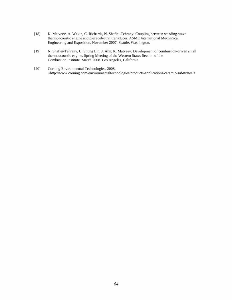
64
[18] K. Matveev, A. Wekin, C. Richards, N. Shafiei-Tehrany: Coupling between standing-wave
thermoacoustic engine and piezeoelectric transducer. ASME International Mechanical Engineering and Exposition. November 2007. Seattle, Washington.
[19] N. Shafiei-Tehrany, C. Shung Lin, J. Ahn, K. Matveev: Development of combustion-driven small
thermoacoustic engine. Spring Meeting of the Western States Section of the Combustion Institute. March 2008. Los Angeles, California.
[20] Corning Environmental Technologies. 2008. <http://www.corning.com/environmentaltechnologies/products-applications/ceramic-substrates/>.