Embed Size (px)
DESCRIPTION
bubbles and structural changes_ france and spain
Citation preview

7/18/2019 bubbles and structural changes_ france and spain
http://slidepdf.com/reader/full/bubbles-and-structural-changes-france-and-spain 1/28
D
I S
C
U
S
S
I O
N
P
A
P
E
R
S E
R
I E
S
Forschungsinstitut
zur Zukunft der ArbeitInstitute for the Study
of Labor
Bubble Economics and Structural Change:
The Cases of Spain and France Compared
IZA DP No. 8942
March 2015
Pablo AgneseJana Hromcová

7/18/2019 bubbles and structural changes_ france and spain
http://slidepdf.com/reader/full/bubbles-and-structural-changes-france-and-spain 2/28
Bubble Economics and Structural Change:The Cases of Spain and France Compared
Pablo AgneseFH Düsseldorf
and IZA
Jana HromcováUniversitat Autònoma de Barcelona
Discussion Paper No. 8942March 2015
IZA
P.O. Box 724053072 Bonn
Germany
Phone: +49-228-3894-0Fax: +49-228-3894-180
E-mail: [email protected]
Any opinions expressed here are those of the author(s) and not those of IZA. Research published inthis series may include views on policy, but the institute itself takes no institutional policy positions.The IZA research network is committed to the IZA Guiding Principles of Research Integrity.
The Institute for the Study of Labor (IZA) in Bonn is a local and virtual international research centerand a place of communication between science, politics and business. IZA is an independent nonprofitorganization supported by Deutsche Post Foundation. The center is associated with the University ofBonn and offers a stimulating research environment through its international network, workshops andconferences, data service, project support, research visits and doctoral program. IZA engages in (i)original and internationally competitive research in all fields of labor economics, (ii) development ofpolicy concepts, and (iii) dissemination of research results and concepts to the interested public.
IZA Discussion Papers often represent preliminary work and are circulated to encourage discussion.
Citation of such a paper should account for its provisional character. A revised version may beavailable directly from the author.

7/18/2019 bubbles and structural changes_ france and spain
http://slidepdf.com/reader/full/bubbles-and-structural-changes-france-and-spain 3/28
IZA Discussion Paper No. 8942March 2015
ABSTRACT
Bubble Economics and Structural Change: The Cases of Spain and France Compared*
This paper delves into the recent events that led to the formation of the housing bubble in
Spain and the resulting structural change that is arguably needed to put the economy backinto the right track. For this purpose we calibrate a model with different equilibria descriptiveof the labor markets in Spain and France, where the unemployment rates went from thesame initial spot to very different levels. In addition to this, we run two counterfactualanalyses that throw some more light on the performance of the Spanish labor market and theSpanish housing bubble. Our results suggest that the unemployment rate in Spain has jumped to much higher levels while switching between equilibria or, what is the same,because of structural change. Moreover, our counterfactuals indicate that, first, the Spanishflexibilization reform has fallen short of its own goals and, second, there has been animportant misdirection of resources into the construction industry mainly fueled byexcessively low real interest rates.
JEL Classification: J64, O57
Keywords: structural change, bubble, unemployment, interest rate, productivity
Corresponding author:
Pablo AgneseFH DüsseldorfDepartment of Business StudiesUniversitätsstraße Geb. 23.32
40225 DüsseldorfGermanyE-mail: [email protected]
* Financial support from the Spanish Ministry of Education and Science through grant ECO2012-37572 is gratefully acknowledged.

7/18/2019 bubbles and structural changes_ france and spain
http://slidepdf.com/reader/full/bubbles-and-structural-changes-france-and-spain 4/28
1 Introduction
In this paper we aim at …nding a possible answer to the structural change that took
place in Spain in recent years, as particularly manifested by the sharp increase in the
unemployment rate to all-time record levels. Spain, unlike many other countries in theEU, embarked, through its banking sector, in a lending spree fueled by the ECB’s lax
monetary policy that ended up in the housing bubble and the subsequent deep recession.
For this we calibrate a model that allows for di¤erent types of equilibria descriptive of
both Spain and France, the latter used as a benchmark country. We complement this
analysis with two counterfactual exercises that throw some more light on the Spanish
labor market and the making of its housing bubble. As it will become evident in the
next pages our paper will go beyond the theoretical framework and will rely, when
possible, on the available data.
Recent developments and growth …gures in Spain and France stand in stark con-
trast.1 While Spain is currently …ghting its way out of a severe and long-lasting reces-
sion, apparently with positive results that indicate a clear change in the trend, France,
on the other hand, is slowing down and even grinding to a halt. But this is just the tip
of the iceberg. Prior to these new events, however, Spain had to undo (and still has to)
much of its previous wrongdoings while aiming its guns on a di¤erent target. Indeed,
austerity measures were joined by a clear consensus that the construction industry could
no longer be the economy’s main driver.
Our contribution in this paper o¤ers a possible answer to what brought these two
countries to their current state of economic a¤airs and the diverging paths undertaken
in both cases. What we contend is that Spain, unlike France, has had to undergo (and
still has) a deep structural change in its productive model—or a switch between di¤erent
equilibria as it will become clear later. This took place basically out of the necessity
to move away from the construction industry and into other more highly value-added
activities.2 The "brick sector", as has been dubbed in Spain, was hailed as the chicken
of the golden eggs during most of the early 2000s. However, as credit became scarce
and investors and construction companies began to pull out of the sector, the economystarted on a downhill slide that was aggravated by the international crisis of 2007–08
and that made the unemployment rate hit new records—26% in 2013 along with more
than 50% youth unemployment.
On the onset of the current crisis both countries were positioned on the same spot in
terms of unemployment. By 2006 both unemployment rates stood at virtually the same
1 See Figure 1 and Table 1 below, as well as Figures 3 through 7 in the next section.2 Such preference has been called out from di¤erent quarters lately, see among many, the OECD
Economic Surveys for Spain (2005, 2014), the OECD Report (2007) on competitiveness and the value
chain, the IMF multi-authored Working Paper on competitiveness in the Southern Euro Area, and theMcKinsey&Company–Fedea Growth Agenda for Spain (2010).
2
7/18/2019 bubbles and structural changes_ france and spain
http://slidepdf.com/reader/full/bubbles-and-structural-changes-france-and-spain 5/28
level, 8.5% according to the OECD Economic Outlook (2014). But the similarities end
right there. Higher GDP growth rates in Spain prior to the crisis were fueled by the
housing bubble which was in turn sparked by the very low interest rate policy of the
European Central Bank. Notice that this "arti…cial" growth brought the unemployment
rate down from "normal" to unprecedented low levels, equaling that of France in 2006.We say unprecedented because the natural or equilibrium rate of unemployment in
Spain has been estimated to be around 14–20% in the years preceding the bubble (see
Estrada et al. 2000, or Mc Morrow and Roeger, 2000). We argue that the sudden
increase of the unemployment rate during and after the crisis was mainly due to a
substantial reallocation of resources. This was the natural consequence of putting all
eggs in one basket. In other words, once the need for a change in the Spanish productive
model became noticeable, it also became self-evident that the transition process towards
another kind of economy was not going to be an easy walk.The reason we focus so eagerly on the Spanish economy responds to what we think is
a major structural change and, as a result, a change in the direction from previous years.
France will only be used as a reference for comparison purposes, mainly to highlight
the notable changes that took place recently in its next-door neighbor. It must be
noted that France, unlike Spain, has not diverted as many resources to the construction
industry during the pre-crisis years and, thus, has not experimented a swift change in
its macroeconomic fundamentals.
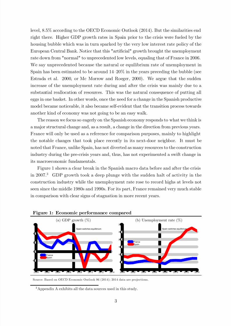
Figure 1 shows a clear break in the Spanish macro data before and after the crisis
in 2007.3 GDP growth took a deep plunge with the sudden halt of activity in the
construction industry while the unemployment rate rose to record highs at levels not
seen since the middle 1980s and 1990s. For its part, France remained very much stable
in comparison with clear signs of stagnation in more recent years.
Figure 1: Economic performance compared
(a) GDP growth (%) (b) Unemployment rate (%)
4
2
0
2
4
6
2000 2002 2004 2006 2008 2010 2012 2014
FranceSpain
Spain switches equilibrium
4
8
12
16
20
24
28
2000 2002 2004 2006 2008 2010 2012 2014
France
Spain
Spain switches equilibrium
Source: Based on OECD Economic Outlook 96 (2014); 2014 data are projections.
3 Appendix A exhibits all the data sources used in this study.
3
7/18/2019 bubbles and structural changes_ france and spain
http://slidepdf.com/reader/full/bubbles-and-structural-changes-france-and-spain 6/28
Table 1 highlights the economic performance of both countries in recent years and
also shows the OECD forecasts for the coming few years. According to the data it
seems that, in both cases, recovery is well under way. We remain, however, a bit
skeptical about the prospect and instead focus alone on the evident change of trend in
the Spanish economy. The year 2014 has been labeled as an in‡ection point towardsthe right economic path,4 as GDP growth went from negative 1.2 to positive 1.3 and
the unemployment rate dropped almost 2 p.p. from a still high 26%.5
Table 1: Economic performance, recent years
2012 2013 2014 2015 2016
(a) GDP growth (%)
France 0.367 0.384 0.371 0.764 1.452
Spain -2.089 -1.230 1.290 1.742 1.947
(b) Unemployment rate (%)
France 9.39 9.85 9.86 10.15 10.05
Spain 24.78 26.09 24.47 23.05 21.93
Source: OECD Economic Outlook 96 (2014); 2014, 2015, 2016 data are projections.
To come to grips with this reversion of the Spanish economy we make use of the equi-
librium and welfare analysis as discussed in Albrecht and Vroman (2002) and Davidson
et al. (2008). Albrecht and Vroman (2002) present a matching model with endogenousskill requirements where employers create both high and low-skill vacancies, and where
it is also assumed that a low-skill job can be done by either type of worker yet high-skill
jobs can only be …lled by high-skill workers. The model suggests that low-skill workers
are generally better o¤ the greater the fraction of low-skill vacancies while the opposite
is true for high-skill workers. Likewise, …rms with low-skill requirements are generally
better o¤ the greater the fraction of low-skill job candidates.
Two equilibria are possible: cross-skill matching (CSM) and ex-post segmentation
(EPS). The equilibrium is of the CSM type when high-skill workers and low-skill vacan-
cies are matched, and EPS when these potential matches do not meet (e.g. high-skill
workers only work in high-skill jobs). Changing the model’s parameters can yield three
scenarios: (i) a CSM-CSM change; (ii) a CSM–EPS switch; and (iii) an EPS–EPS
change. As it will become clear later, only (ii) will be of relevance for us. We argue
that this ‘switch’ between equilibria can be satisfactorily used to explain the structural
4 See the Banco de España Annual Report (2013) for a comprehensive study on the change of coursein the Spanish economy.
5 Indeed, the projected OECD 2014 …gures have been recently supported by the INE (SpanishStatistical O¢ce) and stand at 1.4% for GDP growth and 24.45% for unemployment. French yearly
…gures for 2014 by the INSEE (French Statistical O¢ce) were not available by the time of writing thispaper.
4

7/18/2019 bubbles and structural changes_ france and spain
http://slidepdf.com/reader/full/bubbles-and-structural-changes-france-and-spain 7/28
change taking place in Spain during the crisis years, especially as related to the housing
bubble and the misallocation of resources that resulted from it.
2 Feeding the monkey: The Spanish bubbleDelving into the numbers of the Spanish construction and housing industries might get
us closer to the truth about the recent structural change—or switch between equilibria
to use a more technical term. A smaller economy than its bigger European partners—
with almost only half the population of Germany and three quarters the population of
countries like Italy, France, or the UK—Spain boasted as many as double the workers in
the construction sector as in Germany in 2007, right at the peak of the bubble. Table 2
shows the evolution of construction jobs in major European economies up to the critical
2007 year mark.But what put Spain in this awkward position? What made for the pro‡igacy in
the construction industry, which is clearly re‡ected in the excessive number of jobs
prior to the 2007 crunch? A more than possible yet usually overlooked hypothesis is
that of the booms and busts cycles as laid out by the Austrian School, and recently
discussed by Calvo (2013) in a non-technical paper that goes over the anatomy of crises.
In setting interest rates too low for too long by way of a monetary expansion, central
banks arguably pave the way for higher asset and real estate prices and, eventually, for
overall in‡ation.
6
Following with this reasoning, it is contended that extremely low realinterest rates might divert resources into activities that would not have been targeted
otherwise (e.g. housing). In other words, that due to the arti…cially low cost of credit
resources can be badly allocated, turning the situation into an arti…cial boom—what
Austrians label malinvestment.
Table 2: Construction jobs pre-crisis, Spain in context
2002 2003 2004 2005 2006 2007
Spain 2,189,274 2,310,524 2,455,722 2,657,643 2,797,500 2,880,513
Germany 1,824,337 1,697,818 1,623,974 1,515,465 1,498,760 1,521,752
Italy 1,574,979 1,705,742 1,748,373 1,809,834 1,844,895 1,964,195
France 1,470,596 1,494,723 1,547,648 1,538,128 1,651,546 na
United Kingdom 1,307,459 1,322,636 1,347,409 1,392,009 1,393,461 na
Source: EUROSTAT and INE (2015).
6 For early references on the Austrian School in relation to booms and busts cycles and monetaryexpansion see, most notably, Mises (1912) and Hayek (1931); for other more up-to-date references not
necessarily in line with the Austrians see, for example, Bordo and Landon-Lane (2013) and the onescited in Calvo (2013).
5
7/18/2019 bubbles and structural changes_ france and spain
http://slidepdf.com/reader/full/bubbles-and-structural-changes-france-and-spain 8/28
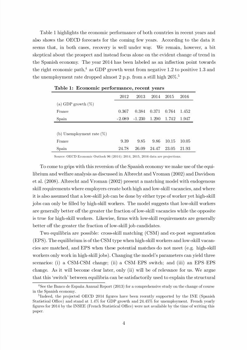
Even when it is not our intention here to analyze this claim further, we think it
provides with a clear and more than reasonable motivation for the structural break
the Spanish economy is currently undergoing. Figure 2 illustrates this ‘break’ to some
extent: mortgages and construction jobs experienced a remarkable growth during the
pre-crisis period which was accompanied with negative real interest rates in most of theyears. This process is now being reverted to some degree after the de‡ationary forces
have set in and have brought interest rates to a higher level. This, however, is not devoid
of serious consequences as spiralling increases in house prices have been combined with
increases in home ownership during the bubble years (see Garriga, 2010)—which, in
turn, plays against those facing mortgage obligations under the new higher interest
rate scenario. Both the long-term interest on Spanish government bonds and the 12-
month Euribor display similar patterns, which were again driven down to very low levels
during 2012–2014 (shown in Figure 3) due to further monetary expansion by the ECBin the face of these "de‡ationary threats".7 ;8
Figure 2: Housing bubble in Spain
Sources: Based on OECD Economic Outlook 96 (2014), Spanish Ministry of Development
and INE (2015), and Bank of Spain (2015).
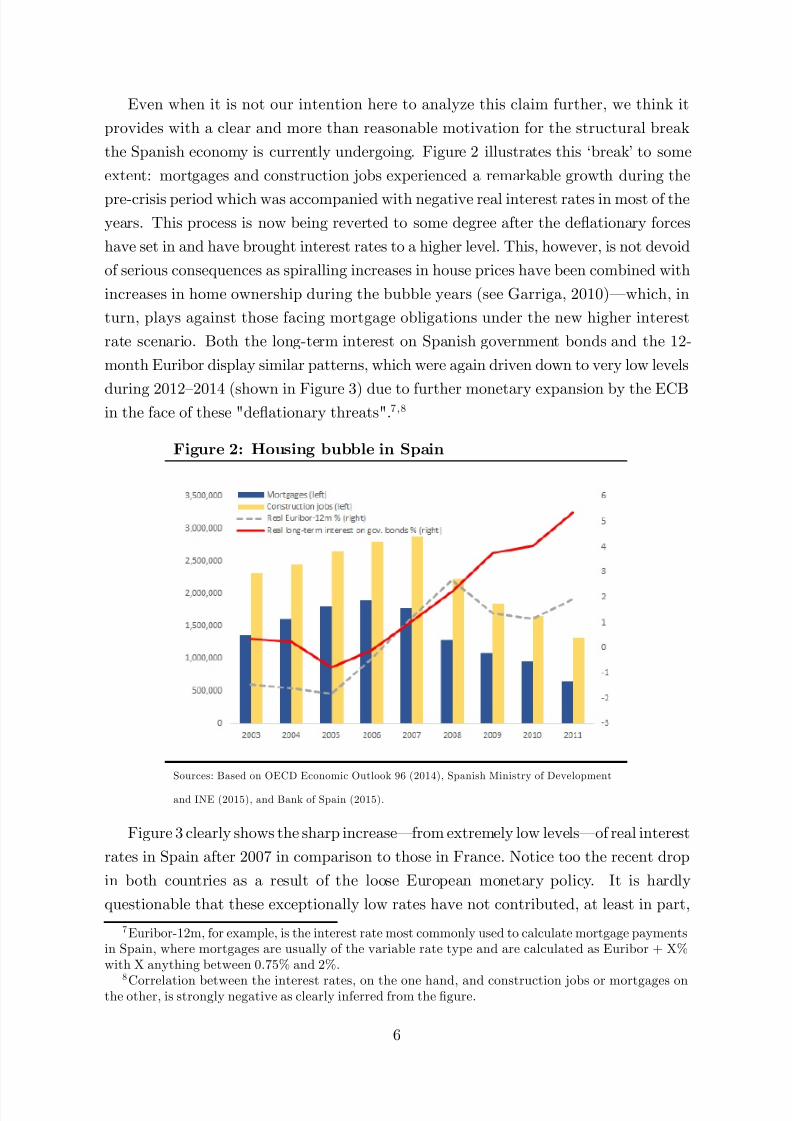
Figure 3 clearly shows the sharp increase—from extremely low levels—of real interest
rates in Spain after 2007 in comparison to those in France. Notice too the recent drop
in both countries as a result of the loose European monetary policy. It is hardly
questionable that these exceptionally low rates have not contributed, at least in part,
7 Euribor-12m, for example, is the interest rate most commonly used to calculate mortgage paymentsin Spain, where mortgages are usually of the variable rate type and are calculated as Euribor + X%with X anything between 0.75% and 2%.
8
Correlation between the interest rates, on the one hand, and construction jobs or mortgages onthe other, is strongly negative as clearly inferred from the …gure.
6
7/18/2019 bubbles and structural changes_ france and spain
http://slidepdf.com/reader/full/bubbles-and-structural-changes-france-and-spain 9/28
to give shape to the housing bubble in Spain. We cannot assess the magnitude of this
phenomenon here, and it is not our goal; rather, we propose a fairly simple setting to
rationalize the structural change in the Spanish economy in terms of a switch between
equilibria.
Figure 3: Real interest rates compared
(a) Long-term government bonds (%) (b) Euribor-12m (%)
1
0
1
2
3
4
5
6
2000 2002 2004 2006 2008 2010 2012 2014
FranceSpain
-2
-1
0
1
2
3
4
2000 2002 2004 2006 2008 2010 2012 2014
FranceSpain
Source: Based on OECD Economic Outlook 96 (2014) and Bank of Spain (2015).
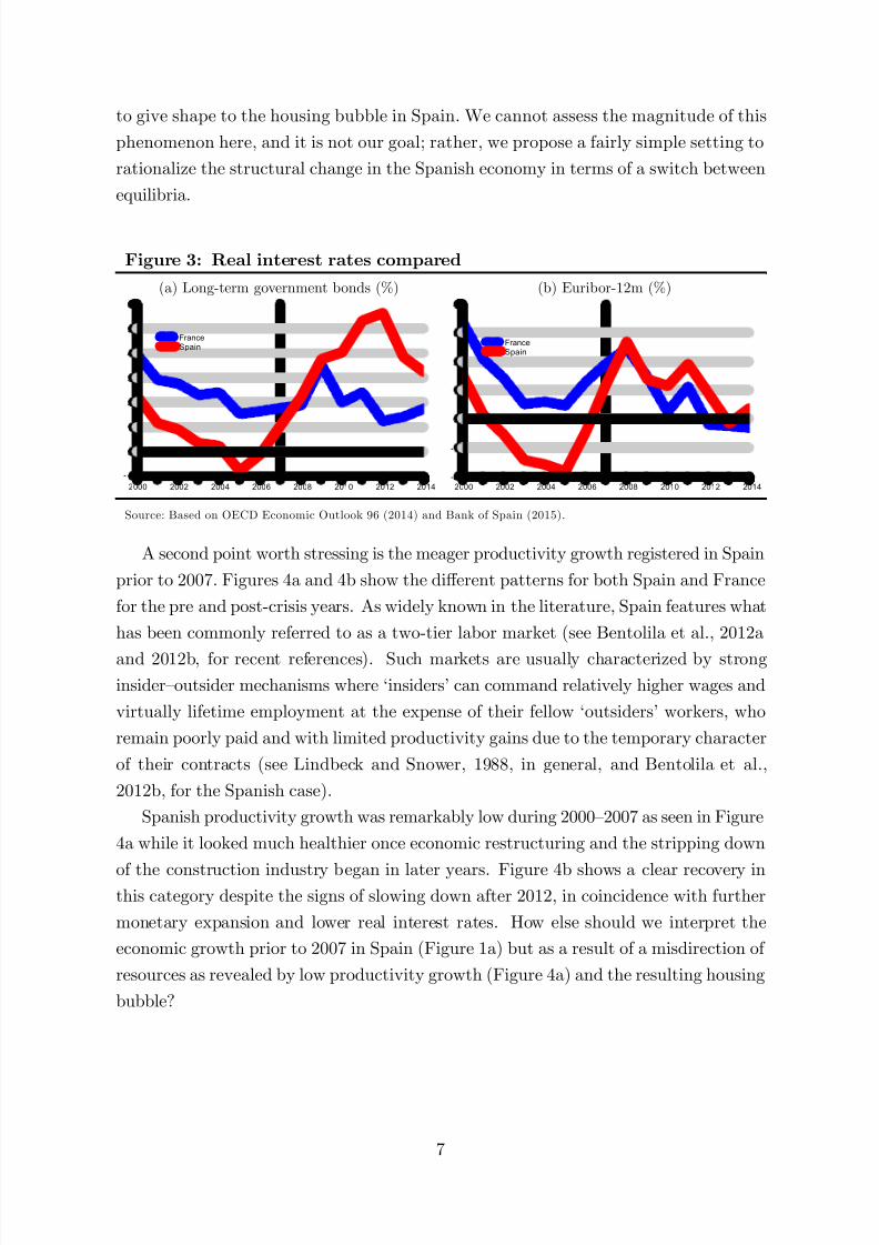
A second point worth stressing is the meager productivity growth registered in Spain
prior to 2007. Figures 4a and 4b show the di¤erent patterns for both Spain and France
for the pre and post-crisis years. As widely known in the literature, Spain features what
has been commonly referred to as a two-tier labor market (see Bentolila et al., 2012a
and 2012b, for recent references). Such markets are usually characterized by strong
insider–outsider mechanisms where ‘insiders’ can command relatively higher wages and
virtually lifetime employment at the expense of their fellow ‘outsiders’ workers, who
remain poorly paid and with limited productivity gains due to the temporary character
of their contracts (see Lindbeck and Snower, 1988, in general, and Bentolila et al.,
2012b, for the Spanish case).
Spanish productivity growth was remarkably low during 2000–2007 as seen in Figure
4a while it looked much healthier once economic restructuring and the stripping down
of the construction industry began in later years. Figure 4b shows a clear recovery inthis category despite the signs of slowing down after 2012, in coincidence with further
monetary expansion and lower real interest rates. How else should we interpret the
economic growth prior to 2007 in Spain (Figure 1a) but as a result of a misdirection of
resources as revealed by low productivity growth (Figure 4a) and the resulting housing
bubble?
7

7/18/2019 bubbles and structural changes_ france and spain
http://slidepdf.com/reader/full/bubbles-and-structural-changes-france-and-spain 10/28
Figure 4: Labor productivity compared
(a) Growth rate, pre-crisis (%) (b) Growth rate, post-crisis (%)
-0.5
0.0
0.5
1.0
1.5
2.0
2.5
2000 2001 2002 2003 2004 2005 2006 2007
France
Spain
-2
-1
0
1
2
3
4
2007 2008 2009 2010 2011 2012 2013 2014
FranceSpain
Source: Based on OECD Economic Outlook 96 (2014).
Another unambiguous indication of the Spanish economy being out-of-step before
2007 is given by the evolution of the unit labor costs—which can be de…ned as theaverage cost of labor per unit of output. Figure 5a presupposes a real disconnect
between workers’ compensations and labor productivity for too many years during
‘bubble times’. Figure 5b instead reverses the previous trend as productivity growth is
now catching up with previous wage hikes.
Figure 5: Unit labor costs compared
(a) Growth rate, pre-crisis (%) (b) Growth rate, post-crisis (%)
1
4
2000 2001 2002 2003 2004 2005 2006 2007
FranceSpain
-4
-2
0
2
4
6
8
2007 2008 2009 2010 2011 2012 2013 2014
FranceSpain
Source: Based on OECD Economic Outlook 96 (2014).
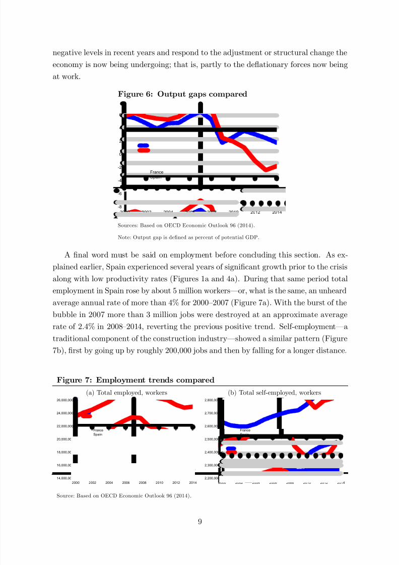
Figure 6 throws more light on the major distortion within the Spanish economy.
The output gap, de…ned as the deviation of actual GDP from potential GDP, as a
percentage of potential GDP, was signi…cantly high in Spain prior to the crisis. The
potential gross domestic product is de…ned by the OECD’s Economic Outlook as the
level of output that an economy can produce at a constant in‡ation rate. Producing
more than the potential level of output, as was the case of Spain before the crisis, comes
at the cost of rising in‡ation, as was also the case there.9 The numbers were reversed to
9 China, too, has recently shown clear signs of overheating, with a housing overstock running up in
the millions, a GDP growth that hasn’t fallen below 7% in the last two decades, and rising commodityprices (especially of food).
8
7/18/2019 bubbles and structural changes_ france and spain
http://slidepdf.com/reader/full/bubbles-and-structural-changes-france-and-spain 11/28
negative levels in recent years and respond to the adjustment or structural change the
economy is now being undergoing; that is, partly to the de‡ationary forces now being
at work.
Figure 6: Output gaps compared
-8
-6
-4
-2
0
2
4
6
2000 2002 2004 2006 2008 2010 2012 2014
France
Spain
Sources: Based on OECD Economic Outlook 96 (2014).
Note: Output gap is de…ned as percent of potential GDP.
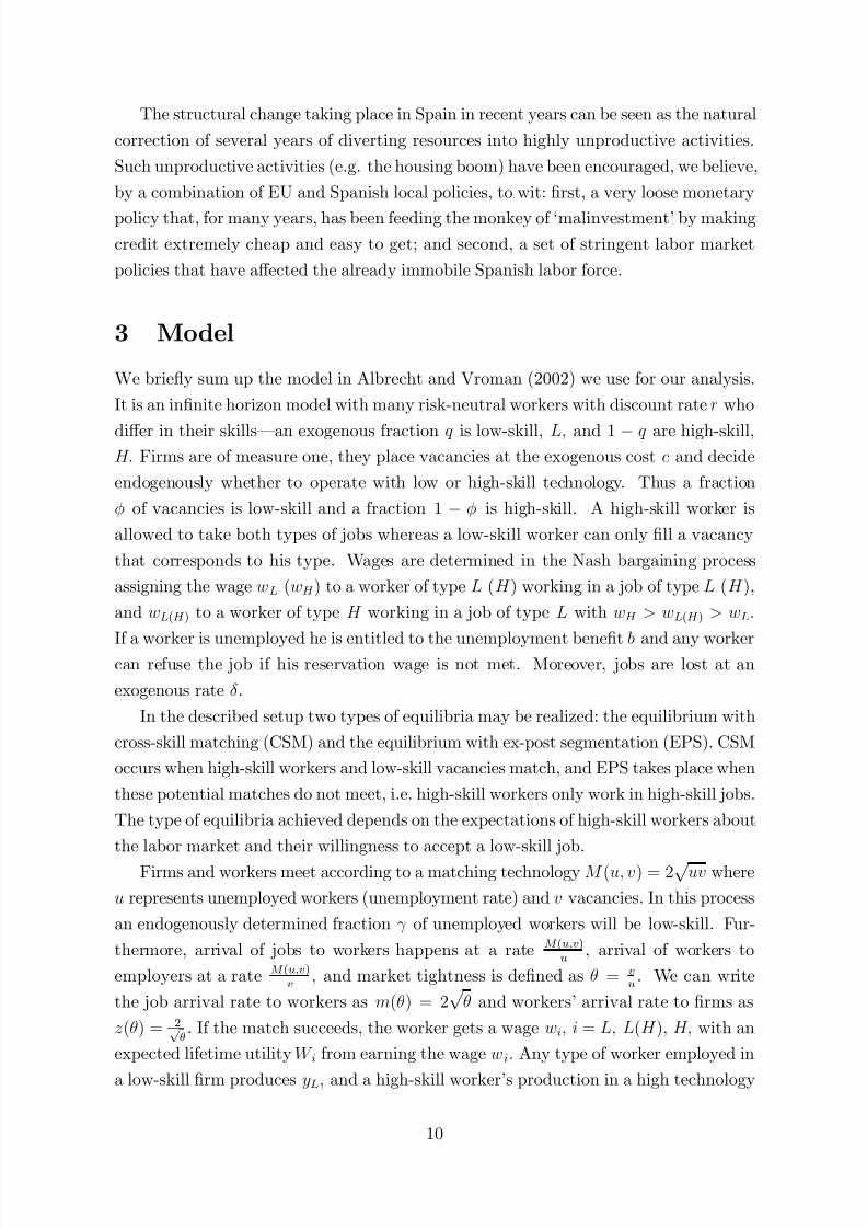
A …nal word must be said on employment before concluding this section. As ex-
plained earlier, Spain experienced several years of signi…cant growth prior to the crisis
along with low productivity rates (Figures 1a and 4a). During that same period total
employment in Spain rose by about 5 million workers—or, what is the same, an unheard
average annual rate of more than 4% for 2000–2007 (Figure 7a). With the burst of the
bubble in 2007 more than 3 million jobs were destroyed at an approximate average
rate of 2.4% in 2008–2014, reverting the previous positive trend. Self-employment—a
traditional component of the construction industry—showed a similar pattern (Figure
7b), …rst by going up by roughly 200,000 jobs and then by falling for a longer distance.
Figure 7: Employment trends compared
(a) Total employed, workers (b) Total self-employed, workers
14,000,000
16,000,000
18,000,000
20,000,000
22,000,000
24,000,000
26,000,000
2000 2002 2004 2006 2008 2010 2012 2014
France
Spain
2,200,000
2,300,000
2,400,000
2,500,000
2,600,000
2,700,000
2,800,000
2000 2002 2004 2006 2008 2010 2012 2014
France
Spain
Source: Based on OECD Economic Outlook 96 (2014).
9
7/18/2019 bubbles and structural changes_ france and spain
http://slidepdf.com/reader/full/bubbles-and-structural-changes-france-and-spain 12/28
The structural change taking place in Spain in recent years can be seen as the natural
correction of several years of diverting resources into highly unproductive activities.
Such unproductive activities (e.g. the housing boom) have been encouraged, we believe,
by a combination of EU and Spanish local policies, to wit: …rst, a very loose monetary
policy that, for many years, has been feeding the monkey of ‘malinvestment’ by makingcredit extremely cheap and easy to get; and second, a set of stringent labor market
policies that have a¤ected the already immobile Spanish labor force.
3 Model
We brie‡y sum up the model in Albrecht and Vroman (2002) we use for our analysis.
It is an in…nite horizon model with many risk-neutral workers with discount rate r who
di¤er in their skills—an exogenous fraction q is low-skill, L; and 1 q are high-skill,H: Firms are of measure one, they place vacancies at the exogenous cost c and decide
endogenously whether to operate with low or high-skill technology. Thus a fraction
of vacancies is low-skill and a fraction 1 is high-skill. A high-skill worker is
allowed to take both types of jobs whereas a low-skill worker can only …ll a vacancy
that corresponds to his type. Wages are determined in the Nash bargaining process
assigning the wage wL (wH ) to a worker of type L (H ) working in a job of type L (H ),
and wL(H ) to a worker of type H working in a job of type L with wH > wL(H ) > wL:
If a worker is unemployed he is entitled to the unemployment bene…t b and any workercan refuse the job if his reservation wage is not met. Moreover, jobs are lost at an
exogenous rate .
In the described setup two types of equilibria may be realized: the equilibrium with
cross-skill matching (CSM) and the equilibrium with ex-post segmentation (EPS). CSM
occurs when high-skill workers and low-skill vacancies match, and EPS takes place when
these potential matches do not meet, i.e. high-skill workers only work in high-skill jobs.
The type of equilibria achieved depends on the expectations of high-skill workers about
the labor market and their willingness to accept a low-skill job.
Firms and workers meet according to a matching technology M (u; v) = 2p uv where
u represents unemployed workers (unemployment rate) and v vacancies. In this process
an endogenously determined fraction of unemployed workers will be low-skill. Fur-
thermore, arrival of jobs to workers happens at a rate M (u;v)u
; arrival of workers to
employers at a rate M (u;v)v
; and market tightness is de…ned as = vu
. We can write
the job arrival rate to workers as m() = 2p
and workers’ arrival rate to …rms as
z () = 2p
. If the match succeeds, the worker gets a wage wi; i = L; L(H ); H; with an
expected lifetime utility W i from earning the wage wi: Any type of worker employed in
a low-skill …rm produces yL; and a high-skill worker’s production in a high technology
10
7/18/2019 bubbles and structural changes_ france and spain
http://slidepdf.com/reader/full/bubbles-and-structural-changes-france-and-spain 13/28
…rm produces yH : Notice that high-skill …rms are more productive than low-skill …rms,
yH > yL, and that the …rms’ pro…ts depend on the level of output and the incurred
costs, namely, wages and searching. Pro…ts are de…ned as yLwLc and yLwL(H )c
in the case that a low-skill …rm employs a low and high-skill worker, respectively, and
yH wH c in the case that a high-skill …rm employs a high-skill worker. We also havethat a …rm’s expected discounted pro…ts are J i; i = L; L(H ); H . Figure 8 sketches the
matches, wages, and output obtained under the two equilibria.
Figure 8: Possible matches between workers and …rms
If the agreement between a worker and a …rm is not achieved, the worker’s income
corresponds to the unemployment bene…t b and his lifetime expected utility is U j; j = L;
H: In such a case, the …rm ends up with an un…lled vacancy of value V j; j = L; H:
We thus have that W i stands for the value of working and U j for the value of unem-
ployment, while J i stands for the value of the job and V j for the value of the vacancyfor the corresponding type. There is something to bargain over if the worker obtains
a positive surplus when working W H U H > 0; W L(H ) U H > 0 and W L U L > 0;
and when the …rm gets positive surplus by hiring the worker, i.e. J H V H > 0; J L(H )V L > 0 and J L V L > 0: Wages are then chosen to maximize the weighted worker’s
and …rm’s surpluses, (W H U H ) (J H V H )
1;
W L(H ) U H
J L(H ) V L1
and
(W L U L) (J L V L)1 ; respectively, where represents the worker’s bargaining power.
Firms enter the market as long as the value of opening a vacancy is non-negative. Once
many …rms enter the market the value of the vacancy hits zero and the process stops—
thus V L = 0 and V H = 0 hold in all periods.
11
7/18/2019 bubbles and structural changes_ france and spain
http://slidepdf.com/reader/full/bubbles-and-structural-changes-france-and-spain 14/28
Workers may experience spells of employment and unemployment. When the ‡ow
of workers into and out of each employment state coincide the steady-state equilibrium
is achieved. Previously employed workers of each type who lose their jobs coincide with
the number of unemployed workers that …nd the job
E L = m() (q E L) ; (1)
E H = m() (1 q E H ) (2)
where E L denotes employed low-skill workers E L = q u; and E H denotes employed
high-skill workers E H = 1 q (1 ) u: Like Albrech and Vroman (2002) we concen-
trate on the steady state equilibrium results. More details on the equilibrium equations
can be found in Appendix B.
4 Results
To make sense of the model above and better understand the housing bubble and struc-
tural change that has recently taken place in Spain we propose three di¤erent exercises.
First, we calibrate the model with real data for France and Spain as these two coun-
tries’ performances, especially in terms of unemployment, stand in stark contrast during
the recent crisis period. We suggest various possibilities concerning the parameters and
equilibria as to make sense of the countries’ diverging unemployment rates.10 Second,
we carry out a …rst counterfactual experiment focusing on the unemployment rate in
Spain and highlighting the e¤ects of the mild ‡exibilization reform undertaken in recent
years. And third, we propose a second counterfactual experiment with an eye on the
interest rate and the making of the Spanish bubble.
One hard piece of evidence worth noting is that both unemployment rates went from
8.5% in 2006 to very di¤erent plateaus in 2013 at the peak of the recession—9.9% in
France and 26.1% in Spain. This is quite a leap indeed for Spain and deserves some
thought. We can summarize our analysis below by arguing, …rst, that a change in
the productivity di¤erential in the calibrated model can lead to a change of equilibria
in Spain as to render the economy quite out of balance (e.g. the burst of bubble
and the ensuing skyrocketing unemployment); second, that the existing labor market
institutions in Spain are not suitable to deal with the unemployment problem and,
moreover, that in the Spanish experience they might have proved highly detrimental as
the economy switched between equilibria; and third, that the housing bubble was, in
all probability, behind the structural change in Spain.
10 Bentolila et al. (2012a) develop a parallel analysis for France and Spain with quarterly data yet
with a focus on the transition between equilibria.
12
7/18/2019 bubbles and structural changes_ france and spain
http://slidepdf.com/reader/full/bubbles-and-structural-changes-france-and-spain 15/28
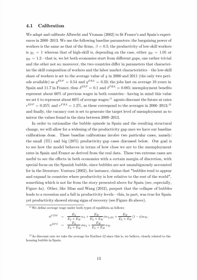
4.1 Calibration
We adapt and calibrate Albrecht and Vroman (2002) to …t France’s and Spain’s experi-
ences in 2000–2013. We use the following baseline parameters: the bargaining power of
workers is the same as that of the …rms, = 0:5; the productivity of low-skill workers
is yL = 1 whereas that of high-skill is, depending on the case, either yH = 1:05 or
yH = 1:2—that is, we let both economies start from di¤erent gaps, one rather trivial
and the other not so; moreover, the two countries di¤er in parameters that character-
ize the skill composition of workers and the labor market characteristics—the low-skill
share of workers is set to the average value of q in 2000 and 2011 (the only two peri-
ods available) as q ESP = 0:54 and q FRA = 0:33; the jobs last on average 10 years in
Spain and 11.7 in France, thus ESP = 0:1 and FRA = 0:085; unemployment bene…ts
represent about 60% of previous wages in both countries—having in mind this value
we set b to represent about 60% of average wages;11 agents discount the future at rates
rESP = 0:35% and rFRA = 1:2%, as these correspond to the averages in 2000–2013;12
and …nally, the vacancy cost is set to generate the target level of unemployment as to
mirror the values found in the data between 2000–2013.
In order to rationalize the bubble episode in Spain and the resulting structural
change, we will allow for a widening of the productivity gap once we have our baseline
calibrations done. These baseline calibrations involve two particular cases, namely:
the small (5%) and big (20%) productivity gap cases discussed below. Our goal is
to see how the model behaves in terms of how close we are to the unemploymentrates in Spain and France as derived from the real data. These two extreme cases are
useful to see the e¤ects in both economies with a certain margin of discretion, with
special focus on the Spanish bubble, since bubbles are not unambiguously accounted
for in the literature. Ventura (2002), for instance, claims that "bubbles tend to appear
and expand in countries where productivity is low relative to the rest of the world",
something which is not far from the story presented above for Spain (see, especially,
Figure 4a). Other, like Miao and Wang (2012), purport that the collapse of bubbles
leads to a recession and a fall in productivity levels—this, in part, was true for Spainyet productivity showed strong signs of recovery (see Figure 4b above).
11 We de…ne average wage under both types of equilibria as follows
wCSM = E L
E L + E H wL +
E H
E L + E H wL(H ) +
E H
E L + E H (1 )wH ;
wEPS = E L
E L + E H wL +
E H
E L + E H wH :
12 As discount rate we take the average for Euribor-12 since this is, we believe, closely related to thehousing bubble in Spain.
13
7/18/2019 bubbles and structural changes_ france and spain
http://slidepdf.com/reader/full/bubbles-and-structural-changes-france-and-spain 16/28
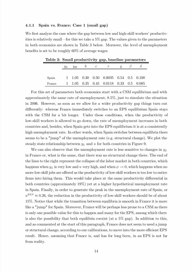
4.1.1 Spain vs. France: Case 1 (small gap)
We …rst analyze the case where the gap between low and high-skill workers’ productiv-
ities is relatively small—for this we take a 5% gap. The values given to the parameters
in both economies are shown in Table 3 below. Moreover, the level of unemployment
bene…ts is set to be roughly 60% of average wages.
Table 3: Small productivity gap, baseline parameters
yL yH b c r q
Spain 1 1.05 0.30 0.50 0.0035 0.54 0.5 0.100
France 1 1.05 0.35 0.45 0.0118 0.33 0.5 0.085
For this set of parameters both economies start with a CSM equilibrium and with
approximately the same rate of unemployment, 8.5%, just to simulate the situation
in 2006. However, as soon as we allow for a wider productivity gap things turn out
di¤erently: whereas France immediately switches to an EPS equilibrium Spain stays
with the CSM for a bit longer. Under these conditions, when the productivity of
low-skill workers is allowed to go down, the rate of unemployment increases in both
countries and, besides, when Spain gets into the EPS equilibrium it is at a consistently
high unemployment rate. In other words, when Spain switches between equilibria there
seems to be a "jump" of the unemployment rate (e.g. structural change). We plot the
steady state relationship between yL and u for both countries in Figure 9.
We can also observe that the unemployment rate is less sensitive to changes in yL
in France or, what is the same, that there was no structural change there. The end of
the lines to the right represent the collapse of the labor market in both countries, which
happens when yL is very low and u very high, and when ! 0, which happens when no
more low-skill jobs are o¤ered as the productivity of low-skill workers is too low to entice
…rms into hiring them. This would take place at the same productivity di¤erential in
both countries (approximately 19%) yet at a higher hypothetical unemployment rate
in Spain. Finally, in order to generate the peak in the unemployment rate of Spain, oruESP 0:26, the reduction in the productivity of low-skill workers should be of about
15%. Notice that while the transition between equilibria is smooth in France it is more
like a "jump" for Spain. Moreover, France will be perhaps less prone to a CSM as there
is only one possible value for this to happen and many for the EPS, among which there
is also the possibility that both equilibria coexist (at a 5% gap). In addition to this,
and as commented at the start of this paragraph, France does not seem to need a jump
or structural change, according to our calibrations, to move into the more e¢cient EPS
result. Hence, assuming that France is, and has for long been, in an EPS is not far
from reality.
14

7/18/2019 bubbles and structural changes_ france and spain
http://slidepdf.com/reader/full/bubbles-and-structural-changes-france-and-spain 17/28
Figure 9: Spain vs. France, small productivity gap
4.1.2 Spain vs. France: Case 2 (big gap)
Our second case depicts the more realistic event of a wider productivity di¤erential
between low and high-skill workers. We here set yH = 1:2 and yL = 1, a 20% produc-
tivity gap. Notice that the parameters used for this calibration shown in Table 4 below
slightly di¤er from those above, mainly due to the fact that we want to guarantee that
bene…ts are roughly 60% of average wages in both countries.
Table 4: Big productivity gap, baseline parameters
yL yH b c r q
Spain 1 1.20 0.32 0.50 0.0035 0.54 0.5 0.100
France 1 1.20 0.40 0.40 0.0118 0.33 0.5 0.085
For this set of parameters both France and Spain start in an EPS equilibrium—
the CSM equilibrium does not exist. Allowing for a 20% gap now suggests that, inorder to achieve the peaks in the unemployment rates in recent years, uESP 0:26 and
uFRA 0:10; the drop in productivity should be of about 13% in Spain and almost
negligible in France. Figure 10 plots the new sets of equilibrium combinations between
yL and u. This is consistent with …ndings in Bentolila et al. (2012a) that the impact of
the recession in Spain was more deeply felt. Again, the end of the lines to the right (low
yL; high u) represent the collapse of the labor market as low-skill vacancies approach
zero. Notice that the Spanish labor market would collapse "earlier" and at a much
higher unemployment rate due to a smaller fraction of high-skill workers.
15

7/18/2019 bubbles and structural changes_ france and spain
http://slidepdf.com/reader/full/bubbles-and-structural-changes-france-and-spain 18/28
Figure 10: Spain vs. France, big productivity gap
4.2 Counterfactuals I: The Spanish labor market
We now proceed with our …rst set of counterfactuals, as we believe it will further our
understanding about the performance of the Spanish labor market after the recent ‡ex-
ibilization reforms. Our strategy goes as follows: we …rst derive an estimable equation
for unemployment from our model above; then we estimate the equation using the
available data; and last, we use the estimated model to obtain the contribution of the‡exibilization variable to the change of the unemployment rate during the recent years.
This contribution is computed through a dynamic simulation of the estimated model
as follows: we …rst …x the exogenous variable at the level of certain arbitrary year, then
we solve the model, and …nally we retrieve the new path of the unemployment rate. For
us, the simulation’s initial year roughly corresponds with the beginning of the global
crisis in Europe—we take 2007 as this year coincides with the lowest of unemployment
in our period of analysis.
It can be demonstrated that the unemployment rate is given by the following generalexpression13
u = f (; q; c; b; r; ; yL; )
where unemployment is dependent on , the rate at which jobs are lost, q , the
share of low-skill workers, c, vacancy costs (more broadly interpreted here as ‘market
‡exibility’), b, the unemployment bene…t, r, the rate at which agents discount the
future, the bargaining power of workers, yL, the productivity of low-skill workers,
13 The unemployment rate as derived from the model above is non-linear and quite burdensome for
estimation purposes. The formal derivation is available on request but we will stick to the linearizedversion as this does not pose a serious drawback for our analysis.
16
7/18/2019 bubbles and structural changes_ france and spain
http://slidepdf.com/reader/full/bubbles-and-structural-changes-france-and-spain 19/28
and , the fraction of low-skill unemployment.
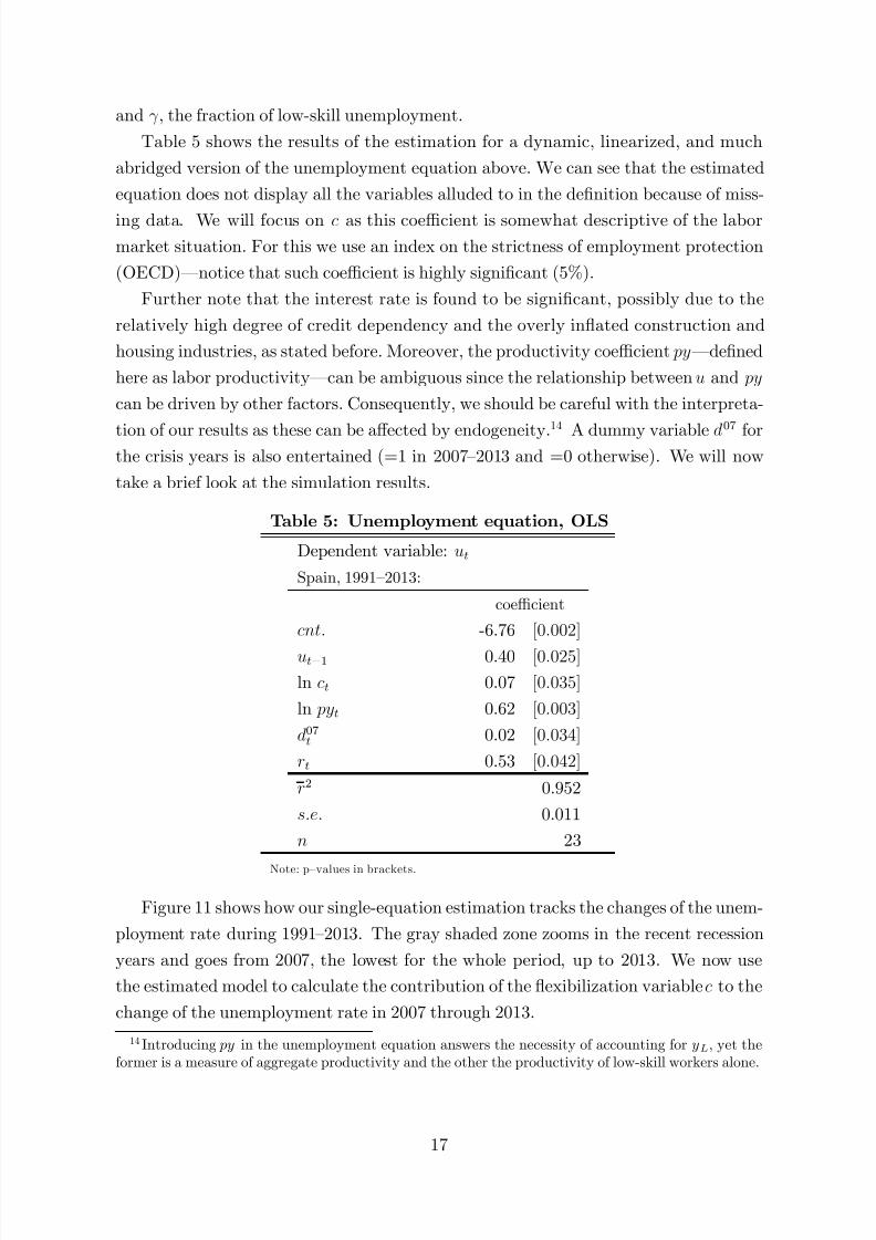
Table 5 shows the results of the estimation for a dynamic, linearized, and much
abridged version of the unemployment equation above. We can see that the estimated
equation does not display all the variables alluded to in the de…nition because of miss-
ing data. We will focus on c as this coe¢cient is somewhat descriptive of the labormarket situation. For this we use an index on the strictness of employment protection
(OECD)—notice that such coe¢cient is highly signi…cant (5%).
Further note that the interest rate is found to be signi…cant, possibly due to the
relatively high degree of credit dependency and the overly in‡ated construction and
housing industries, as stated before. Moreover, the productivity coe¢cient py—de…ned
here as labor productivity—can be ambiguous since the relationship between u and py
can be driven by other factors. Consequently, we should be careful with the interpreta-
tion of our results as these can be a¤ected by endogeneity.14
A dummy variable d07
forthe crisis years is also entertained (=1 in 2007–2013 and =0 otherwise). We will now
take a brief look at the simulation results.
Table 5: Unemployment equation, OLS
Dependent variable: ut
Spain, 1991–2013:
coe¢cient
cnt: -6.76 [0:002]
ut1 0.40 [0:025]
ln ct 0.07 [0:035]
ln pyt 0.62 [0:003]
d07t 0.02 [0:034]
rt 0.53 [0:042]
r2 0.952
s:e: 0.011
n 23
Note: p–values in brackets.
Figure 11 shows how our single-equation estimation tracks the changes of the unem-
ployment rate during 1991–2013. The gray shaded zone zooms in the recent recession
years and goes from 2007, the lowest for the whole period, up to 2013. We now use
the estimated model to calculate the contribution of the ‡exibilization variable c to the
change of the unemployment rate in 2007 through 2013.
14 Introducing py in the unemployment equation answers the necessity of accounting for yL, yet theformer is a measure of aggregate productivity and the other the productivity of low-skill workers alone.
17

7/18/2019 bubbles and structural changes_ france and spain
http://slidepdf.com/reader/full/bubbles-and-structural-changes-france-and-spain 20/28
Figure 11: Unemployment rate (%)
4
8
12
16
20
24
28
1992 1996 2000 2004 2008 2012
Actual Fitted
We …x c to the simulation’s starting year, 2007, and solve the model accordingly.
Once we do this we are able to recover the new (simulated) path of the unemployment
rate. Figure 12 is very revealing on the ‘what ifs’ regarding the policy measures related
to c and labor market performance in general. Figure 12 (a) shows the path of the
unemployment rate had the employment protection indicator remained at the level of
2007 (in red), along with the actual trajectory (in blue). As shown there, ‡exibilization
has contributed to a reduction of the unemployment rate of approximately 1.1 p.p..
Unlike a comparative statics exercise our simulation here takes account of the dynamics
occurring within the subsample 2007–2013, and therefore the …nal e¤ect on u is the
result of this summation of e¤ects—even when this is only seen from 2010 onwards,
when the …rst steps were taken in the direction of labor ‡exibilization. Figure 12 (b)
exhibits both the evolution of this variable as well as its simulated path …xed at 2007.
According to our analysis here the Spanish ‡exibilization reform has thus fallen short
of achieving a real improvement of the current conditions.
Figure 12: Labor ‡exibility and unemployment in Spain
(a) Unemployment rate (%) (b) Strictness indicator (0=‡exible to 6=tight)
8
12
16
20
24
28
2007 2008 2009 2010 2011 2012 2013
Actual trajectory
Simulated (employment protection,indicator kept at 200 7--10 value)
8.3
26.4
27.5
2.04
2.08
2.12
2.16
2.20
2.24
2.28
2.32
2.36
2007 2008 2009 2010 2011 2012 2013
Actual tr ajectory
Fixed at 20082.35
2.04
18

7/18/2019 bubbles and structural changes_ france and spain
http://slidepdf.com/reader/full/bubbles-and-structural-changes-france-and-spain 21/28
4.3 Counterfactuals II: The Spanish bubble
We undertake a separate yet similar counterfactual exercise in this section to throw some
light on the role played by interest rates in the building-up of the Spanish bubble during
the early years of the current century. As before, we follow the same methodological
procedure regarding estimation and simulations, with the exception that we now have
no theoretical derivation of the estimable equation. Moreover, our database at this
point is rather limited and we should remain on the conservative side when reading
through our simulations.
Table 6 shows two similar regressions, with the share of construction jobs on total
employment being regressed upon the real interest rate and the output gap. Panel (a)
on the left has the euribor-12 as a regressor whereas panel (b) on the right has the rate
on government bonds. Both coe¢cients are highly signi…cant and negatively signed,
something which is clearly consistent with the story related earlier—that is, very low
interest rates are a major driver behind the malinvestment and redirection of resources
into the in‡ated construction industry.
In addition to the interest rate, the output gap is included as a regressor to highlight
the overheating of the Spanish economy. Signi…cant and positive coe¢cients in both
equations are suggestive of a positive correlation between ‘going beyond the means’
and the housing bubble. In other words, this variable accounts for factors leading to the
housing bubble and the increase of construction employment other than those brought
about by very low interest rates.
Table 6: Construction jobs share equation, OLS
Dependent variable: st
(a) Spain, 2002–2011: (b) Spain, 2002–2011:
coe¢cient coe¢cient
cnt: 0.11 [0:000] cnt: 0.13 [0:000]
reur12t -0.76 [0:000] rgovt -0.94 [0:001]
ogapt 0.71 [0:000] ogapt 0.24 [0:091]
r2 0.969 0.950
s:e: 0.004 0.006
n 10 10
Note: p–values in brackets.
Figure 13 exhibits the actual and …tted patterns of the construction employment
share in those key years of the housing bubble. The drop is quite remarkable after 2007
and the …t quite good for both equations in spite of the few observations involved. In
the next few paragraphs we will be using the estimated model to assess the contribution
of the exogenous variables to the drop in the construction share.
19

7/18/2019 bubbles and structural changes_ france and spain
http://slidepdf.com/reader/full/bubbles-and-structural-changes-france-and-spain 22/28
Figure 13: Construction jobs share
(a) Construction share (%), Euribor equation (b) Construction share (%), Gov. bonds equation
7
8
9
10
11
12
13
14
15
2002 2003 2004 2005 2006 2007 2008 2009 2010 2011
Actual Fitted
7
8
9
10
11
12
13
14
15
2002 2003 2004 2005 2006 2007 2008 2009 2010 2011
Actual Fitted
Figure 14 reveals the contributions of the real interest rates in both equations to the
drop in construction employment. In both cases the contribution was far from negligible,especially for the rate on government bonds. Respectively, these contributions amount
to 1.8 p.p. and 5.1 p.p. for equations in panels (a) and (b).
Figure 14: Contribution of interest rates to the construction share
(a) Construction share (%), Euribor equation (b) Construction share (%), Gov. bonds equation
7
8
9
10
11
12
13
14
15
16
2006 2007 2008 2009 2010 2011
Actual tra jectory
Simulated (euribor-12 kept at 2006 value)14
9
7.2
7
8
9
10
11
12
13
14
15
16
2006 2007 2008 2009 2010 2011
Actual tra jectory
Simulated (gov. bonds rate kept at 2006 value)
14
12.3
7.2
Figure 15 shows the actual and simulated trajectories of the interest rates under
consideration. Notice that, for practical reasons, the simulations had to be run start-
ing in 2006—right during the time when the change in the interest rates was clearly
observed, going from negative in 2006 to positive in 2007 for both rates.
20

7/18/2019 bubbles and structural changes_ france and spain
http://slidepdf.com/reader/full/bubbles-and-structural-changes-france-and-spain 23/28
Figure 15: Interest rates, actual and simulated
(a) Euribor-12 (%) (b) Gov. bonds rate (%)
-0.5
0.0
0.5
1.0
1.5
2.0
2.5
3.0
2006 2007 2008 2009 2010 2011
Actual trajectory
Fixed at 2006
1.92
-0.44-1
0
1
2
3
4
5
6
2006 2007 2008 2009 2010 2011
Actual tr ajectory
Fixed at 2006
5.34
-0.1
The size of the contributions is switched for the next simulation, where we assess
the e¤ect of economic overheating by way of the output gap on the construction share.
While the output gap for the Euribor equation in panel (a) of Figure 16 shows acontribution of 5.4 p.p. in the drop of the employment share, the contribution for the
government bonds equations in (b) stands at 1.8 p.p..
Figure 16: Contribution of other factors to the construction share
(a) Construction share (%), Euribor equation (b) Construction share (%), Gov. bonds equation
7
8
9
10
11
12
13
14
15
2007 2008 2009 2010 2011
Actual trajectory
Simulated (output gap kept at 200 7 value)
14 12.6
7.2
7
8
9
10
11
12
13
14
15
2007 2008 2009 2010 2011
Actual trajectory
Simulated (output gap kept at 2 007 value)
14
9
7.2
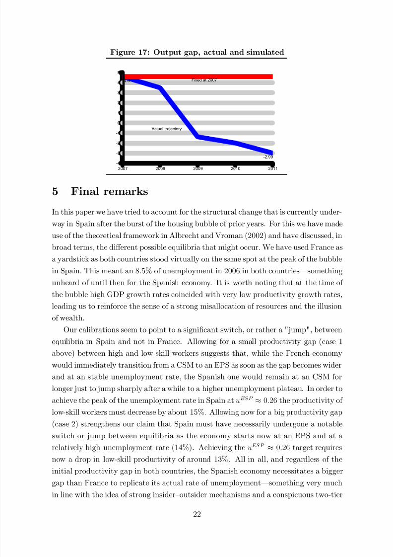
Further notice that if we add both contributions in each one of the equations they
roughly add to the total drop in employment—which was approximately of the order
of 7 p.p. between 2006–7 and 2011, as seen in Figure 13 above. These numbers are nottrivial since total employment in Spain went down by 2.2 millions during that period
and the employment in the construction industry shrank by 1.5 millions from almost 3
millions—or a 50% drop. Finally, Figure 17 shows the actual and simulated trajectory
of the output gap for both equations.
21
7/18/2019 bubbles and structural changes_ france and spain
http://slidepdf.com/reader/full/bubbles-and-structural-changes-france-and-spain 24/28
Figure 17: Output gap, actual and simulated
-4
-3
-2
-1
0
1
2
3
4
5
2007 2008 2009 2010 2011
Actual trajectory
Fixed at 20074.6
-2.99
5 Final remarksIn this paper we have tried to account for the structural change that is currently under-
way in Spain after the burst of the housing bubble of prior years. For this we have made
use of the theoretical framework in Albrecht and Vroman (2002) and have discussed, in
broad terms, the di¤erent possible equilibria that might occur. We have used France as
a yardstick as both countries stood virtually on the same spot at the peak of the bubble
in Spain. This meant an 8.5% of unemployment in 2006 in both countries—something
unheard of until then for the Spanish economy. It is worth noting that at the time of
the bubble high GDP growth rates coincided with very low productivity growth rates,
leading us to reinforce the sense of a strong misallocation of resources and the illusion
of wealth.
Our calibrations seem to point to a signi…cant switch, or rather a "jump", between
equilibria in Spain and not in France. Allowing for a small productivity gap (case 1
above) between high and low-skill workers suggests that, while the French economy
would immediately transition from a CSM to an EPS as soon as the gap becomes wider
and at an stable unemployment rate, the Spanish one would remain at an CSM for
longer just to jump sharply after a while to a higher unemployment plateau. In order toachieve the peak of the unemployment rate in Spain at uESP 0:26 the productivity of
low-skill workers must decrease by about 15%. Allowing now for a big productivity gap
(case 2) strengthens our claim that Spain must have necessarily undergone a notable
switch or jump between equilibria as the economy starts now at an EPS and at a
relatively high unemployment rate (14%). Achieving the uESP 0:26 target requires
now a drop in low-skill productivity of around 13%. All in all, and regardless of the
initial productivity gap in both countries, the Spanish economy necessitates a bigger
gap than France to replicate its actual rate of unemployment—something very much
in line with the idea of strong insider–outsider mechanisms and a conspicuous two-tier
22

7/18/2019 bubbles and structural changes_ france and spain
http://slidepdf.com/reader/full/bubbles-and-structural-changes-france-and-spain 25/28
labor market in Spain. Arguably, Spain has jumped from a CSM to an EPS in the
post-bubble years while France has either smoothly transitioned from one to the other
(case 1) or, more likely, has always been at an EPS (case 2).
To complement our previous analysis we have carried out two sets of counterfactuals
exercises descriptive of the Spanish labor market and of the Spanish bubble episode. The…rst results are indicative of a move in the good direction by the Spanish government,
which has however fallen short of achieving a major change for the better—‡exibilization
has brought Spanish unemployment down but there is still a long way to go. The
second results stress the misdirection of resources into the construction industry that
were mainly fueled by very low (even negative) real interest rates for the most part of
the last decade. We get to explain the whole change in the construction jobs share by
way of the real interest rate and the output gap—the latter being broadly identi…ed
with additional factors pointing in the direction of economic overheating.
References
[1] Albrecht, James and Vroman, Susan, 2002. A Matching Model with Endogenous
Skill Requirements, International Economic Review 43 (1), 283–305.
[2] Banco de España, 2014. Annual Report 2013, Madrid, ISSN: 1579 - 8623 (online
edition).
[3] Bentolila, Samuel, Cahuc, Pierre, Dolado, Juan J., and Le Barbanchon, Thomas,
2012a. Two-Tier Labour Markets in the Great Recession: France Versus Spain,
The Economic Journal 122 (562), 155–187.
[4] Bentolila, Samuel, Dolado, Juan J., and Jimeno, Juan F., 2012b. Reforming an
insider-outsider labor market: The Spanish experience, IZA Journal of European
Labor Studies 1:4.
[5] Bordo, Michael D. and Landon-Lane, John, 2013. Does Expansionary MonetaryPolicy Cause Asset Price Booms: Some Historical and Empirical Evidence, NBER
Working Paper No. 19585.
[6] Calvo, Guillermo, 2013. Puzzling over the Anatomy of Crises: Liquidity and the
Veil of Finance, Bank of Japan IMES Discussion Paper 13-E-09.
[7] Davidson, Carl, Matusz, J. Steven, and Shevchenko, Andrei, 2008. Outsourcing
Peter to pay Paul: High-skill Expectations and Low-skill Wages with Imperfect
Labor Markets, Macroeconomic Dynamics 12 (4), 463–479.
23

7/18/2019 bubbles and structural changes_ france and spain
http://slidepdf.com/reader/full/bubbles-and-structural-changes-france-and-spain 26/28
[8] Estrada, Angel, Hernando, Ignacio and López-Salido, J. David, 2000. Measuring
the NAIRU in the Spanish Economy, Banco de España Working Papers #0009.
[9] Garriga, Carlos, 2010. The role of construction in the housing boom and bust in
Spain. FEDEA Working Papers 2010-09.
[10] Hayek, Friedrich A. von, 1931, reprint 2008. Prices and Production and Other
Works On Money, the Business Cycle, and the Gold Standard, Auburn, AL: Ludwig
von Mises Institute.
[11] IMF (various authors), 2008. Competitiveness in the Southern Euro Area: France,
Greece, Italy, Portugal, and Spain, IMF WP 08/112.
[12] Lindbeck, Assar and Snower, Dennis, 1988. The Insider-Outsider Theory of Em-
ployment and Unemployment, MIT Press.
[13] McKinsey&Company–Fedea (various authors), 2010. A Growth Agenda for Spain.
[14] Mc Morrow, Kieran and Roeger, W., 2000. Time-Varying NAIRU/NAWRU Esti-
mates for the EU’s Member States, ECFIN Economic Paper No. 145.
[15] Miao, Jianjun, and Wang, Pengfei, 2012. Bubbles and Total Factor Productivity,
American Economic Review 102 (3), 82–87.
[16] Mises, Ludwig von, 1912, reprint 1981. The Theory of Money and Credit, Indi-anapolis, IN: Liberty Fund.
[17] OECD Economic Surveys Spain (various authors), 2005, 2014. ISSN 0376-6438.
[18] OECD Report (various authors), 2007. Staying Competitive in the Global Econ-
omy: Moving Up the Value Chain, OECD Publishing ISBN 9264034250.
[19] Ventura, Jaume, 2002. Bubbles and Capital Flows, NBER Working Papers 9304.
24

7/18/2019 bubbles and structural changes_ france and spain
http://slidepdf.com/reader/full/bubbles-and-structural-changes-france-and-spain 27/28
A Appendix: Data sources
Table A: Data sources
Real GDP growth (%) OECD Economic Outlook 96 (2014).
Unemployment rate (%) OECD Economic Outlook 96 (2014).Construction jobs EUROSTAT and INE (2015).
Mortgages INE (2015).
Real long-term interest on gov. bonds (%) OECD Economic Outlook 96 (2014).
Real Euribor–12 months (%) Bank of Spain (2015).
Labor productivity, growth rate (%) OECD Economic Outlook 96 (2014).
Unit labor costs, growth rate (%) OECD Economic Outlook 96 (2014).
Output gap (%) OECD Economic Outlook 96 (2014).
Total and self-employment data OECD Economic Outlook 96 (2014).
Note: Both real interest rates de‡ated by gross domestic product de‡ator, market prices (OECD).
B Appendix: CMS and EPS equations
We outline all the equations that must hold in CSM and EPS equilibria.
Cross-skill matching equilibrium:
Bellman equations of employed workers are
rW L = wL (W L U L); (3)
rW L(H ) = wL(H )
W L(H ) U H
; (4)
rW H = wH (W H U H ): (5)
Bellman equations that characterize the unemployed workers are
rU L = b + m() (W L U L) ; (6)
rU H = b + m()[W L(H ) + (1 )W H U H ]: (7)
Bellman equations for the active …rms are
rJ L = (yL wL c) (J L V L) ; (8)
rJ L(H ) =
yL(H ) wL(H ) c [J L(H ) V L]; (9)
rJ H = (yH wH c) (J H V H ) : (10)
25

7/18/2019 bubbles and structural changes_ france and spain
http://slidepdf.com/reader/full/bubbles-and-structural-changes-france-and-spain 28/28
Corresponding equations for inactive …rms are
rV L = c + z ()
J L + (1 )J L(H ) V L
; (11)
rV H = c + z ()(1 ) (J H V H ) : (12)
Wages are set in the Nash bargaining process as
wL = (yL c) + (1 )rU L; (13)
wL(H ) = (yL c) + (1 )rU H ; (14)
wH = (yH c) + (1 )rU H : (15)
Zero vacancy conditions, V L = V H = 0, (1) and (2) must also hold. Cross-skill matching
equilibrium will exist if yL c > rU H : (16)
Ex-post segmentation equilibrium:
Bellman equations that characterize the employed workers are (3) and (5), corre-
sponding equations for unemployed workers are (6) and
rU H = b + (1 )m() (W H U H ) : (17)
Bellman equations for the active …rms are (8) and (10), and for the inactive …rms are
rV L = c + z () (J L V L) (18)
and (12).15 Zero vacancy conditions, V L = V H = 0, (1) and (2) must also hold. The
condition for the existence of the EPS equilibrium implies that high-skill workers are
matching only with high-skill jobs
yL c rU H : (19)
15
Notice that equations (17) and (18) now imply that high-skill unemployed workers will only takehigh-skill jobs and low-skill …rms will ony hire low-skill workers.