Bridging genetic networks and queueing theory - TAUuriy/Papers/Bridging-genetic-networks-and... · A. Arazi et al./Physica A 332 (2004) 585–616 587 The tools suppliedby queueing

Available online at www.sciencedirect.com

Physica A 332 (2004) 585–616www.elsevier.com/locate/physa

Bridging genetic networks and queueing theoryArnon Arazia, Eshel Ben-Jacobb;∗, Uri Yechialia

aDepartment of Statistics & Operations Research, School of Mathematical Sciences,Raymond & Beverly Sackler Faculty of Exact Sciences, Tel-Aviv University, Tel-Aviv 69978, Israel

bSchool of Physics and Astronomy, Raymond & Beverly Sackler Faculty of Exact Sciences,Tel-Aviv University, Tel-Aviv 69978, Israel

Abstract

One of the main challenges facing biology today is the understanding of the joint actionof genes, proteins and RNA molecules, interwoven in intricate interdependencies commonlyknown as genetic networks. To this end, several mathematical approaches have been introducedto date. In addition to developing the analytical tools required for this task anew, one canutilize knowledge found in existing disciplines, specializing in the representation and analysisof systems featuring similar aspects. We suggest queueing theory as a possible source of suchknowledge. This discipline, which focuses on the study of workloads forming in a variety ofscenarios, o7ers an assortment of tools allowing for the derivation of the statistical properties ofthe inspected systems. We argue that a proper adaptation of modeling techniques and analyticalmethods used in queueing theory can contribute to the study of genetic regulatory networks. Thisis demonstrated by presenting a queueing-inspired model of a genetic network of arbitrary sizeand structure, for which the probability distribution function is derived. This model is furtherapplied to the description of the lac operon regulation mechanism. In addition, we discuss thepossible bene8ts stemming for queueing theory from the interdisciplinary dialogue with molecularbiology—in particular, the incorporation of various dynamical behaviours into queueing networks.c© 2003 Elsevier B.V. All rights reserved.

PACS: 87.22.B; 02.50.H; 87.10

Keywords: Genetic networks; Queueing theory; G-Networks; Product form; Periodic behaviour

1. Introduction

With the completion of several genome sequencing projects, concerning variousorganisms (see for examples Refs. [1–4]), increasing attention is now turned to the

∗ Corresponding author. Tel.: +972-3-6407845; fax: +972-3-642-5787.E-mail address: [email protected] (E. Ben-Jacob).

0378-4371/$ - see front matter c© 2003 Elsevier B.V. All rights reserved.doi:10.1016/j.physa.2003.07.009

mailto:[email protected]

586 A. Arazi et al. / Physica A 332 (2004) 585–616

understanding of the interactions between genes, proteins and RNA molecules [5].In particular, the regulation of gene expression is studied extensively. Alongside themore orthodox biological methods, mathematical tools are applied for the gaining ofboth qualitative and quantitative insights into regulatory systems (see Refs. [6,7] forsurveys).Although such e7orts have now seen their fourth decade, no single modeling frame-

work seems to capture all of the observed aspects of genetic regulatory networks [8].The use of di7erential equations for their description (see Ref. [9] for a pioneeringwork), the most common approach employed so far, has been criticized for assum-ing that the modeled quantities change continuously, whereas in reality the inspectedprocesses usually involve small numbers of molecules. Boolean networks [10], anotherwidespread formalism, were argued against for viewing genes as binary elements, be-ing either “o7” or “on”; while this can be considered as an acceptable approximationfor some genes, it has been shown that there are occasions where intermediate levelsof expression should be regarded explicitly. Both approaches have been criticized fortreating genetic networks as deterministic mechanisms, ignoring the stochastic noiseintrinsic to them.During the last decade, the use of discrete and probabilistic models for the descrip-

tion of genetic networks has become increasingly popular. As the analytical investi-gation of such schemes is quite complicated, most researchers employ simulations intheir study (see, for example, Ref. [11]). Even so, some analytical results have beenobtained (e.g. [12–15]).In this paper we suggest the use of queueing theory for the study of genetic networks.

Queueing theory is a branch of Operations Research, dedicated to the study of systemsof queues, or workloads, forming in various scenarios; usually, these are assumed toincorporate stochastic phenomena. A well-established 8eld, it has been successfullyutilized for the modeling and analysis of several real-world problems.Generalizing the standard concepts of queueing theory, a queue can be considered

as the accumulation of customers, due to a series of random events, whose occur-rence is subject to the set of rules de8ning the system. The customers can representpractically anything—people standing on a line in front of a clerk, airplanes waitingto land, computer jobs waiting to receive CPU time, etc. We suggest here to usethis general notion for the representation of molecules of some sort. In this case, thequeue length is simply the number of such molecules currently present in the system.Alternatively, one can view the queue length as something more abstract, such as theexpression level of some gene; a customer then represents a “notch” in the scale of geneactivity.Integrating multiple, interconnected queues in such a model, leads to a representation

of the interactions of several types of molecules and genes. A customer moving fromone queue to another due to service completion, can represent the formation of onetype of molecule due to some chemical reaction involving the other (e.g., the actionof a certain enzyme).The direct result of applying this modeling scheme is the description of the regulatory

network as a discrete, stochastic, asynchronous system. As mentioned above, such adescription is well in accordance with current views regarding these networks.

A. Arazi et al. / Physica A 332 (2004) 585–616 587

The tools supplied by queueing theory allow for the derivation of the long-termstatistical properties of such systems, as well as their dependence on parameter valuesand on the con8guration of queue interactions. Such insights can prove to be extremelyuseful to the understanding of genetic regulatory systems.The harnessing of queueing theory to the study of genetic networks can take two

forms. One may choose to adopt an existing queueing model, out of the exceedinglywide array of models studied over the years, changing its interpretation to match thebiological scene of interest; the immediate bene8t from such an approach is the readyvalidity of existing results found for the original model, in the biological context.Alternatively, an acquaintance with the analytical methods used in queueing theory maybe sought; these can be later employed in the study of similar models, tailor-made forthe exact biological system at hand.Some reservations must be noted, however. Most of the results obtained in queueing

theory are analytical, backed-up by rigorous mathematical proofs. While this is a majoradvantage, it also poses restrictions regarding the changes and adjustments that can bemade in a given model, without losing the validity of the results. In addition, at leastgenerally speaking, the requirement for mathematical strictness usually accompanyingqueueing theory, limits the complexity and intricacy of the scenarios that can be handledby its tools.Finally, it is worth mentioning that some of the analytical work done in the stochas-

tic modeling of genetic networks came close to queueing theory, in that some of theassumptions made (namely those regarding the Markovian character of the processesinvolved), as well as some of the analytical methods employed in these works, coincidewith subsets of queueing theory. In one case (and, to our knowledge, the only case),an explicit analogy was drawn between the model studied and a model taken fromqueueing theory [13]; doing so, the authors were able to prove that their model con-verges to a steady state distribution in an exponential rate. However, we are unawareof a more thorough attempt to draw lines of similarity between the two 8elds.We also argue that bridging between queueing theory and computational biology

can prove to be bene8cial for the former as well. Using approximation schemes ofstochastic systems, it is possible to derive queueing networks roughly depicting vari-ous dynamical behaviours, such as periodical cycles or chaos. While the mathematicalknowledge allowing for this possibility has existed for some time, queueing theoryliterature does not contain examples of such behaviours. To produce these, one canrely on existing dynamical models, and in particular, models describing the dynamicsof genetic networks. We suggest that the employment of dynamical systems theory ingeneral, and that of dynamical genetic networks in particular, can signi8cantly enrichthe study of queueing systems.The organization of this paper is as follows. Section 2 provides an overview intro-

ducing queueing theory, with examples of some of the themes and models studied, aswell as some of the results obtained. Section 3 presents the notion of genetic networks,and reviews the main approaches employed in their modeling, the emphasis being ondiscrete stochastic models. Section 4 discusses the use of queueing theory for the mod-eling of genetic networks. An example of a speci8c model, stemming from such anapproach, is given; as a demonstration of the kind of results it produces, this model


is later applied for the description of the lac operon regulation mechanism. The 8nalsection regards the construction of queueing networks displaying various dynamicalbehaviours; an example of this is supplied.

2. Queueing theory

2.1. The basics

Queueing theory (see, for example Refs. [16,17]) is one of the subjects exploredwithin the discipline of Operations Research. As the name implies, its main objects ofinterest are queues, or work loads, forming in front of servers of some sort. It has itsroots early in the twentieth century, in the work of the Danish engineer A.K. Erlang,who studied traOc loads occurring in telephone systems. Since then it has developedto answer various real-world challenges, stemming from a variety of areas such as thedesign and management of industrial production lines, telephony systems, computernetworks, motorized vehicles traOc and more, being successful in presenting new so-lutions. For example, the protocols implemented in the ALOHANET and ARPANETcomputer networks, which constitute the basis for today’s Internet, were designed andanalyzed using queueing theory. In order to address the complex nature of such scenar-ios, an extensive arsenal of mathematical tools has been devised, most of them generalenough to be utilized in an assortment of di7erent problems.The simplest queueing scheme—that of a single service facility—is described in

Fig. 1. In this scheme, customers requiring service enter the queueing system and jointhe queue, waiting to be served. From time to time, a customer standing in the queue isselected for service according to some prede8ned policy. The required service is thenperformed, after which the customer leaves the queueing system. Note that, given thewide variety of problems handled by queueing theory, it should be clear that the termsused—“customers”, “service” and so on—are general and metaphoric in their essence.Usually, the arrival of customers and their service are considered to be the out-

come of stochastic processes. Making speci8c assumptions regarding the distributionfunctions of these processes enables one to build mathematical probabilistic modelsfor the analysis of the queueing system. These, in turn, allow for the derivation ofcertain characteristics, such as the average queue length, the average waiting time of acustomer, the average time required to clear the system out of customers, and so on.Queueing theory mainly focuses on the steady state of the inspected system. That

is, it is assumed that after a suOcient time, the queueing system stabilizes, and its state(usually de8ned as the number of customers in it) becomes essentially independent ofits initial conditions. Note that this does not mean that the queueing system reaches a8xed state; rather, it obtains a 8xed (or stationary) distribution function describing itsstate—a distribution that does not change over time.Below is considered a series of representative examples, demonstrating common

models explored by queueing theory, as well as some of the results obtained; theseexamples will also assist us in establishing our ideas, further below. We open with twomodels of single queues, and continue to discuss networks of queues.


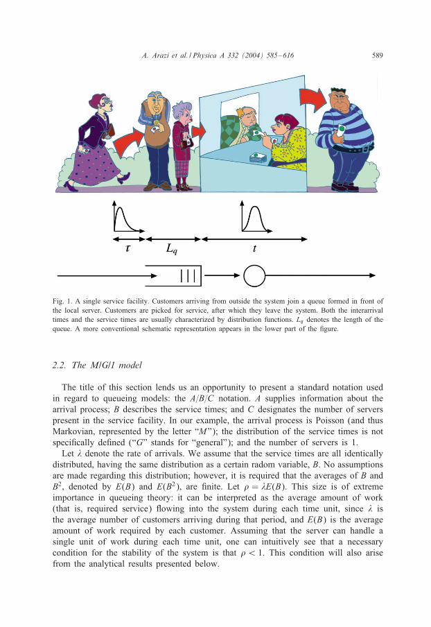
Fig. 1. A single service facility. Customers arriving from outside the system join a queue formed in front ofthe local server. Customers are picked for service, after which they leave the system. Both the interarrivaltimes and the service times are usually characterized by distribution functions. Lq denotes the length of thequeue. A more conventional schematic representation appears in the lower part of the 8gure.

2.2. The M/G/1 model

The title of this section lends us an opportunity to present a standard notation usedin regard to queueing models: the A=B=C notation. A supplies information about thearrival process; B describes the service times; and C designates the number of serverspresent in the service facility. In our example, the arrival process is Poisson (and thusMarkovian, represented by the letter “M”); the distribution of the service times is notspeci8cally de8ned (“G” stands for “general”); and the number of servers is 1.Let denote the rate of arrivals. We assume that the service times are all identically

distributed, having the same distribution as a certain radom variable, B. No assumptionsare made regarding this distribution; however, it is required that the averages of B andB2, denoted by E(B) and E(B2), are 8nite. Let � = E(B). This size is of extremeimportance in queueing theory: it can be interpreted as the average amount of work(that is, required service) Sowing into the system during each time unit, since isthe average number of customers arriving during that period, and E(B) is the averageamount of work required by each customer. Assuming that the server can handle asingle unit of work during each time unit, one can intuitively see that a necessarycondition for the stability of the system is that �¡ 1. This condition will also arisefrom the analytical results presented below.


In order to analyze this model, one can use the fact that the arrival process is Poisson,and de8ne a Markov chain embedded in the moments of service completion. Let Xnbe the number of customers present in the system at the moment the nth customercompletes his service; and let �n be the number of customers arriving to the systemduring the service of the nth customer. It follows that

Xn+1 = Xn − 1 + �n+1 if Xn¿ 0

and

Xn+1 = �n+1 if Xn = 0 :

The reason for this is as follows: If the system was not empty after the departure ofthe nth customer (that is, Xn¿ 0), then the number of customers in it after the nextservice completion, is the number of customers present when that service began, minus1 (the (n+ 1)th served customer), plus the customers arriving during that service. If,on the other hand, the nth customer left no customers behind him, then the (n+ 1)thcustomer reaches an empty system, receives service, and leaves behind him only thecustomers arriving during his service.Using this recursive rule, it is possible to derive the Laplace–Stieltjes transform of

X , de8ned as X (s)=E[eSX ]. Relying again on the Poisson nature of the arrival process,one can show that the distribution of X , the number of customers in the system at themoments of service completion, is the same as the distribution of L, the number ofcustomers in the system at an arbitrary moment. One can then proceed to deduce themean of L, given by the so-called Pollaczek-Khintchine formula:

E(L) =2E(B2)2(1− �)

+ � : (1)

We can see that indeed, as � → 1; E(L) → ∞, and the system loses its stability.A less intuitive result is the dependence of L on the second moment (and hence, thevariance) of the service times distribution. This means that it is not enough to rely ona calculus of averages alone to describe the behaviour of a queueing system; variancesmust be considered as well.There is a wealth of other results that can be found for this model. However, we

will settle with what was presented, and proceed to the next example.

2.3. The M/M/1 model

Here we look at a scenario identical to the previous one, but further assume thatthe distribution of the service times is exponential, with a rate denoted by � (thus,the events of service completion are generated by a Markovian process. This explainsthe second “M” in the notation used for this case). This additional assumption enablesthe derivation of more detailed results, most notably an explicit expression of thedistribution function of L. However, this assumption may be diOcult to justify in somecases.Again, we set �= E(B). Here, E(B) = 1=�, so �= =�.


The analysis of the M=M=1 system is conducted in a di7erent manner than that ofthe M=G=1 model. The system is described using a birth-and-death process, where abirth stands for the arrival of a customer, and a death for a departure of a customer(after service completion). One can then show that the stationary probability of havingk customers in the system is equal to

P(L= k) = (1− �)�k (2)

(conditioned that �¡ 1).In particular, P(L = 0) = 1 − �, or, alternatively, P(L¿ 0) = �. This gives another

interpretation to the meaning of �—the proportion of time during which the server isbusy serving customers.Some of the additional results obtainable here are the average number of customers

in the system, and the average time a single customer spends in the system (denotedby W ):

E(L) =�

1− �=

� −

; (3)

E(W ) =1

� − : (4)

Furthermore, one can show that the probability distribution function of W is expo-nential with a rate equal to (� − ), namely P(W 6 t) = 1− e−(u−)t .

2.4. Networks of queues and product form solutions

Queueing theory analysis is not limited to the case of a single service facility; onepossible complication is the consideration of a network of queues. Such a network iscomposed of multiple service facilities, each with its own queue and server. 1 Cus-tomers may generally arrive from outside the system to any of these facilities. Aftera customer is served, he can either leave the system or move to a di7erent facility inthe network, joining the queue there. The possible movements between the queues 2 —usually described by transition probabilities, speci8ed separately for each queue—de8nethe structure of the network.Queueing networks are rather diOcult to explore, and in order to enable some sort

of analysis to be conducted, one must usually assume that all of the distributionsinvolved—both of the interarrival times and the service times—are exponential. Furtherassuming that the rates of these distributions are constant, results in a family of models

1 Note that it is possible to derive analytical results in the case where multiple servers are present in aservice facility, as well. However, we will restrict our discussion here to the case of a single server in eachfacility.

2 That is, movements between service facilities. In what follows, the term “queue” will be used to denoteboth the service facility, and the queue in it—in accordance with the conventional terminology used inrelation to queueing networks.


Fig. 2. Two queues in a Jackson network. The 8gure displays the possible transitions, together with theirrates and probabilities. Each queue is denoted by a circle and each transition is denoted by an arrow. Theservice rates are written inside the circles; the arrival rates, in front of arrows; probabilities, beside arrows.

named Jackson networks. In these networks, it is possible to derive an explicit ex-pression of the stationary joint distribution function of the queue lengths—that is, onecan precisely 8gure the probability that in the 8rst queue there will be k1 customers,in the second queue k2 customers, etc. Furthermore, this distribution function has aparticular form, called product form: it can be written as the product of n components,n being the number of queues in the network, where each component complies withthe marginal distribution function of a single queue. This allows not only for the ex-ploration of the joint behaviour of the network, but also for the separate analysis ofeach single queue. We will brieSy show all this now.Let �i be the rate of arrivals to the ith queue, from outside the system; and let �i be

the service rate at facility i. When a customer completes his service there, he moves toqueue j with probability pij, or leaves the system with probability di = 1−∑n

j=1 pij.This scheme is presented in Fig. 2.We further de8ne the aggregate input rates in each queue—that is, the rate of

arrivals to the queue, both from the outside and from other queues in the network. Theaggregate arrival rate to queue i is denoted by i. It follows that:

i = �i +n∑

j=1

jpji = �i +n∑

j=1

�j�jpji; i = 1; : : : ; n ; (5)

where �i=i=�i. These n linear equations are called the tra@c equations of the network.Note that as in the M=M=1 and M=G=1 models, �j represents the proportion of timeduring which the server in queue j is busy. Thus, �j�j is the eAective service rate atqueue j, and �j�jpji is the e7ective passage rate from queue j to queue i.The so-called Jackson Theorem states that the stationary joint probability distribution

of the system is given by

P(L1 = k1; : : : ; Ln = kn) =n∏i=1

(1− �i)�kii : (6)

The condition for stability is �i ¡ 1; ∀i.Indeed, one can see that the joint probability distribution is presented as the product

of n components, each depending on the parameters of a single queue only (once theaggregate rates have been computed, that is). This allows for the conclusion of the


marginal probability distribution function of each queue, as well as its average length:

P(Li = ki) = (1− �i)�kii ; (7)

E(Li) =�i

1− �i: (8)

Comparing these results to those obtained in the M=M=1 model, it is possible to see thatonce the aggregate rates have been computed (taking into account the interdependenciesof queues in the network), each queue can be statistically treated as if it were a separateM=M=1 system, standing on its own.

2.5. G-Networks

G-networks (the “G” stands for “generalized”), 8rst presented by Gelenbe in theearly 1990s [18], are an extension of Jackson networks. Here, two types of elementsmove around in the network: Customers, which are identical to the customers in regularqueueing networks; and signals, which induce some e7ect on the queues of the network,and then leave the system. The exact nature of this e7ect di7ers in the various typesof G-networks: signals can cause a single customer to leave the system (in which casethey are sometimes called “negative customers”); they can trigger the movement ofa customer from one queue to another; or they can cause the deletion of a randomamount of work from a queue—these are but a few of the signals types studied so far(for surveys of papers exploring G-networks, see Refs. [19,20]). Signals can appearfrom outside the network; or they can be a result of a “metamorphosis” occurring toa regular customer.A common result recurring in the study of G-networks, is that of product form

stationary solutions—as with Jackson networks. However, in G-networks, the traOcequations, used here for the description of the aggregate rates of customer arrivals aswell as those of signal arrivals, are generally nonlinear; this poses questions regardingthe existence of such solutions (note that uniqueness is derived automatically fromexistence, since we are dealing here with the normalized stationary solution of a systemof Chapman-Kolmogorov equations—see also Ref. [19]).Most of the applications of G-networks explored to date refer to computer networks,

where cancellation of work, as well as the movement of work from one server toanother, is indeed possible—for example, as part of load balancing schemes. Anotherapplication—the one that initially motivated the use of G-networks—is the modelingof neural networks. In this context, a service facility represents a neuron; the length ofthe queue represents the activation level of the neuron; the movement of a customerfrom one service facility to another represents the excitation of the latter neuron bythe former; and the movement of a signal, which has the e7ect of removing a sin-gle customer from the target queue, represents inhibition. For further information, seeRefs. [19,21,22].Thus, G-networks constitute a convenient framework for modeling rather general

phenomena—that of stochastic processes involving the coupled increase and decreaseof some studied amounts (which can be represented by the queue lengths), organizedin some prede8ned structure. This framework can be applied to a wide range of cases.


However, at least to our knowledge, G-networks were not yet used for the descriptionof biochemical or genetic networks.

2.6. Approximations of queueing networks

Finding an explicit expression of the joint distribution function of a queueingnetwork is usually possible only in the simplest cases, e.g. when one considers thestationary distribution and assumes Bxed rates for the stochastic processes involved.For more complicated scenarios, it is still possible to write an integro-di7erential equa-tion describing the time evolution of the network’s transition probabilities: this is thewell-known Kolmogorov forward integro-diAerential equation, also called the mas-ter equation of the network [23]. Solving this equation supplies the time-dependentjoint probability distribution function of the network; however, this is generally adiOcult task.An alternative way to write the master equation is to use the Kramers–Moyal ex-

pansion [24,25]. Here, the time derivatives of the transition probabilities are expressedusing an in8nite series involving the moments of the distribution function of the jumpprocess. This does not necessarily simplify the solution of the equations, but it readilyleads to an approximation scheme, namely keeping only the leading terms in the series.Taking into account only the 8rst term in the series results in what is known as the

Cuid approximation, which approximates the average behaviour of the system overtime, employing a deterministic description. Such an approximation is usually validonly when the changes induced by the movement of a single customer are relativelynegligible compared to the overall network’s state. In addition, if the Suid approxima-tion features more than one stable steady state, its validity is limited to a certain timeinterval.When one keeps the 8rst two terms in the Kramers–Moyal expansion, the result is a

diAusion equation. Its solution approximates the transition probability density functionof the system, so that the statistical properties of the system can be assessed.

3. Genetic networks

3.1. Biological motivation

The main functions in a living cell are carried out by proteins, which are synthesizedfrom the information kept in its genes. Though all the cells in an organism contain thesame DNA (with few exceptions), di7erent cells express di7erent genes and producedi7erent proteins, therefore exhibiting di7erent behaviours. Thus, in order to understandthe cell’s functioning, one cannot settle for acquiring knowledge of the DNA sequencesalone, but must also become acquainted with the processes regulating protein synthesis,determining which protein will be produced and when, and at what level [6].A key feature of these regulatory processes is the fact that they themselves involve

the utilization of proteins. For example, proteins may act as enhancers or repressors ofthe expression of speci8c genes (possibly the genes which are responsible to their own


production), controlling the amount of mRNA transcribed from them; and the synthesisof these regulatory proteins themselves may be controlled by yet other proteins. Thisgives rise to an intricate network of regulatory interactions between DNA, RNA, pro-teins and small molecules, sometimes referred to as a genetic network. Through thesenetworks, the organism can implement complicate logical “circuits”, which enable itto respond appropriately to various environmental conditions. A well-studied exampleis the relatively simple network, which enables E. coli to produce the metabolic en-zymes required for the digestion of lactose, only in the absence of the more favourableglucose [5,26].Since the interactions comprising a genetic network may be fairly complex, includ-

ing interlocking positive and negative feedback loops, mere intuition usually does notsuOce for understanding their behaviour. Rather, formal mathematical methods andcomputer tools are required for their modeling, analysis and simulation, as means ofgaining some insight into their functioning.More speci8cally, such approaches are useful for several purposes. First, there are

certain regulatory circuits, extensively studied over the years, for which most elementsparticipating in the regulatory processes, as well as the interactions between them, havebeen identi8ed. For these cases, detailed models can be built and studied, shedding newlight on the possible dynamics that can arise, their robustness to changes in certainconditions, etc. The results of such an analysis may pose new questions and point toareas where more experimental work is needed, which can lead to more accurate andspeci8c models, and so forth.A second use for modeling and analysis is the study of general structural mo-

tifs, which are recurrent in several regulatory circuits (for example, negative feedbackloops). The exploration of general motifs may result in a more profound understandingof regulatory networks in general (see Ref. [27] for an example of this approach).Third, recent years have seen the rise of such laboratory techniques as microarray

technology, which allow for the simultaneous measurement of the expression levels ofmany genes. One possible use for such data is the reverse-engineering of the underly-ing genetic network, through the use of statistical inference methods (see, for example,Ref. [28]). However, these methods may result in several candidate networks. Incor-porating the knowledge gained from the study of regulatory circuits dynamics mayenhance such a research process, helping to disqualify unsuitable networks.Over the past 40 years, various approaches have been suggested for studying regu-

latory networks, each with its own strengths and weaknesses. Most of these focus onthe 8rst point of regulation, i.e., that of gene expression (protein synthesis is regulatedat each of its steps—gene expression, RNA processing and transport, RNA transla-tion, and posttranslational modi8cations of proteins). Here we discuss some of theseapproaches, in particular those which are more closely related to the one suggested byus. We base our discussion on Refs. [6,7], which contain more elaborate surveys.

3.2. Boolean networks

Boolean networks were 8rst suggested as a model of genetic regulatory systems byKau7man, in 1969 [10]. In this approach, it is assumed that in order to e7ectively


describe the behaviour of such systems, it is suOcient to consider explicitly only theexpression levels of genes, without specifying the concentrations of mRNA molecules,proteins and other participants in the modeled processes. The state of a gene is approx-imated by a Boolean variable—that is, a gene can be either “on” (currently expressed)or “o7” (currently silenced). The regulatory control of the expression of each gene isrepresented by a logical function, depending on the states of other genes in the net-work. For example, such a function may specify that gene A will be “on” in the nexttime step if currently gene B is “on” and gene C is “o7”. As implied in this example,the states of the genes in the network are updated in discrete time steps; moreover, ineach time step the state of every gene in the network is updated. Thus, all networkelements are assumed to change synchronously.

Since the number of elements in a Boolean network is 8nite, and since each elementhas a discrete number of possible states, the number of possible network states (de8nedas the vector of the states of the individual elements) is also 8nite; thus, a speci8c runof a network is bound to return to a state it already encountered. Also, since all statetransitions are deterministic, the system will then reconstruct all its steps since the 8rstappearance of the recurrent state. Thus, the network is said to have reached a cycle.If this cycle consists of a single state, it is termed a steady state of the system.At the price of making somewhat radical assumptions regarding the nature of gene

expression and its regulation, the Boolean networks approach allows for the study ofextremely large genetic networks, due to its computational simplicity: already in the late1960s, Kau7man was able to inspect networks containing up to 10,000 elements. Suchlarge networks are way beyond the reach of any other existing modeling technique,even today.The study of Boolean networks is performed using computer simulations. These allow

for the identi8cation of steady states and cycles, and of their domains of attraction (thatis, states which lead to these attractors). One research direction concerns studying theimplications of local properties and structural motifs, such as the average connectivityof each element in the network or the logical functions used, on the global behaviourof the network (see Refs. [29–33] for reviews).For example, Kau7man [10] showed that the average connectivity a7ects the length

and stability of cycles in the network.The simplicity of Boolean networks, and the relatively low number of parame-

ters involved in their de8nition, make them attractive models for the purpose ofreverse-engineering the structure of a genetic network out of actual gene-expressiondata (cf. Ref. [34]). However, here their deterministic nature may pose a problem, dueto the noise inherent in real-life gene-expression data [35,36].Almost all of the assumptions made by the Boolean networks approach draw criticism

[8]. First, though it is acceptable, in many cases, to regard gene expression as having abinary nature, as the activation pro8le of genes commonly has the shape of a sigmoidcurve, it is not always appropriate to do so; there are cases where intermediate levels ofgene expression cannot be neglected, as these have a di7erent e7ect than very low orvery high expression levels. Also, the description of gene expression regulation usinglogical functions has been pointed out to be an oversimpli8cation. Third, the assumptionthat all elements change synchronously is problematic, as this is not usually the case,


and as it prevents from certain behaviours from happening [6,7]. In addition, the factthat Boolean networks lack speci8c modeling of the role played by mRNA molecules,proteins and other molecules in gene regulation, makes them unsuitable for describingvarious phenomena [7]. Finally, the assumption of determinism is challenged; this isdiscussed below.

3.3. The “continuous” approach

Under this title we group several works, all using di7erential equations to describethe time evolution of gene expression levels and the amounts or concentrations ofmRNA, proteins and other molecules. All of the involved variables are non-negative andcontinuous. The regulatory interactions are expressed using functional and di7erentialrelations between the variables.Such methods have been widely used for the modeling of genetic regulatory systems,

starting from 1963 [9]; see Refs. [6,7] for a partial list of works. Models were built todescribe either speci8c regulatory circuits, or for the study of general motifs and char-acteristics recurring in a large number of known regulatory systems, such as negativefeedback loops. The interactions considered can be either linear or nonlinear (the lattermore realistic and widespread). Some models take into account the spatial variation,using partial di7erential equations; others use time delays for the same purpose. Severaltypes of behaviour were described using continuous models: steady states, limit cycles,chaos, bistability and multistability, and more.Due to the nonlinearity of most models, numerical simulations are used for their

analysis, rather than analytical methods. In addition, bifurcation analysis is commonlyused for the investigation of the sensitivity of steady states and limit cycles to changesin parameter values.The main advantage of this approach is the ability to accurately model the quantities

described and their interactions. Also, it makes available to the researcher the extensiveknowledge and methodologies of dynamical systems theory.The main disadvantage is the high computational cost involved in running the nu-

merical simulations required. This considerably limits the size of the systems that canbe explored using this approach. In addition, building a complete model requires theaccurate knowledge of the functional interactions between the described molecules,as well as the precise assessment of the involved parameter values. The absence ofsuch data may seriously cripple the model, as the derived behaviours are usually quitesensitive to these speci8cations.

3.4. Probabilistic models

The continuous approach assumes that the modeled amounts vary continuously anddeterministically. However, in the context of gene regulation, these assumptions may beinappropriate, for two reasons: 8rst, the number of molecule instances participating insuch processes may be quite small—few tens of molecules in some cases; and second,some of the chemical reactions involved occur at slow rates. The 8rst point suggeststhat discrete variables may be more 8tting for the representation of molecules amounts;


the second implies the existence of stochasticity in genetic regulatory systems. Indeed,for the latter claim, experimental evidence exists for some time (see Refs. [37,12] fora more elaborate discussion). For example, in phage , the choice between the lyticand lysogenic outcome is probabilistic in its essence, and was successfully modeled assuch in Ref. [11]. Thus, the fate of the entire organism may lie on a single roll of adice.This leads us to the discrete, probabilistic modeling approach. Here, the state of the

system is de8ned as the number of molecules of each type, and is expressed usinga vector of integer, non-negative variables. The possible chemical reactions are de-termined, together with the probability of each reaction to occur (these probabilitiesmay be state-dependent). From these de8nitions stems implicitly the joint probabilitydistribution of the system, which speci8es the probability of a certain state to occur ata certain time. The time evolution of the joint distribution is governed by the masterequation of the system; solving it produces the explicit functional form of this distri-bution, thus giving a complete description of the system’s stochastic behaviour overtime.Unfortunately, in most cases it is quite diOcult to derive the exact form of the master

equation, let alone solve it. Thus, most researchers resort to the use of simulations ofthe explicit molecular interactions occurring in the regulation process, disregarding themaster equation altogether. Even so, some analytic work on the subject exists (seebelow).Stochastic simulations use the framework suggested by Gillespie in 1977 [38]. In

each step, two choices are made randomly, according to the state-dependent probabil-ities speci8ed by the model: the next reaction to occur, and the time on which it willtake place. The state of the system is then updated accordingly, and the simulationproceeds to the next step. This framework was later modi8ed and improved by otherauthors, for example in Ref. [39].A single run of a stochastic simulation will produce an arbitrary trajectory in the

phase space. In order to derive general results concerning the stochastic behaviour ofthe system, several such runs must be performed. It is then possible to get an estimateof the joint probability distribution, as well as the average trajectory and the dispersalaround it.The main advantage of the stochastic simulations approach is the ability to construct

accurate models for the molecular processes involved in gene expression regulation,taking into account all the details held relevant while not neglecting such e7ects asstochasticity. However, exaggerating in this perspective will limit the ability to makeuseful interpretations of the results.From the requirement to execute numerous simulation runs, and from the detailed

description of the chemical reactions involved, usually incorporated in such models,stems the main disadvantage of this approach—its high computational cost. In addition,as with the continuous approach, an exact knowledge of the reaction rates and indeed,of the reaction mechanisms themselves, is required; however, such knowledge is oftenunavailable.As mentioned above, some analytical results were obtained for probabilistic

models of genetic networks, mostly in recent years. In some of these works, it was


possible to derive, and even solve, the master equation itself; others use approximationschemes, based mainly on the Kramers–Moyal expansion. Following is a sample ofthese works.Peccoud and Ycart [13] suggested the use of Markovian birth-and-death processes

to model a single gene and the protein it produces. The gene can be either “on” or“o7”, while the amount of protein molecules is described using an integer, non-negativevariable. The possible transitions in this model are the activation and deactivation of thegene, the production of a protein molecule (if the gene is active), and the degradationof a protein molecule (if the number of these molecules is greater than 0). The rate ofdegradation is linear in the number of protein molecules; all other rates are constant.The model does not include an explicit description of the regulation of the gene (thatis, it is not related to the protein molecules). The authors were able to derive thetime-dependent mean and variance of the number of protein molecules in the system,as well as those in steady state.Kepler and Elston [12] considered a similar model, but examined additionally a

gene enhancing its own production, and a system composed of two mutually repress-ing genes. Again, all reactions are considered to be Markovian, with a linear ratedescribing the degradation of the protein, and 8xed rates for all other interactions.The activation and repression of the gene result from an interaction of two proteinmolecules, so their rate is quadratic in the number of molecules. In the case of theself-enhancing gene, the authors were able to write the di7usion approximation of themaster equation, and to derive from it an approximation of the stationary distributionfunction of the number of protein molecules. They then used this distribution functionto generate a bifurcation diagram, depicting regions of qualitatively di7erent steadystate distributions, as a function of the model parameter values; in addition, they ex-plored the 8rst-passage times between alternative stable steady states. In the case of thetwo mutually repressing genes, the authors conducted a similar analysis, but instead ofusing a di7usion approximation, they approximated the number of protein moleculesusing a set of deterministic ODEs, and generated a bifurcation diagram using these.The analytical results were veri8ed using numerical simulations.Thattai and van Oudenaarden [14] presented a general framework for the treatment

of regulatory networks, consisting of an arbitrary number of genes. Each gene is rep-resented by a triplet of non-negative integers, specifying the numbers of DNA, mRNAand protein molecules (the number of DNA molecules can be used to represent the geneactivation level). The state of the entire network is the collection of all these triplets.The possible stochastic transitions—all Markovian—are an increment or a decrementin the amount of a single molecule. The state-dependent rates of these transitions areassumed to be linear combinations of the numbers of molecules present. The authorsmanaged to obtain the explicit form of the master equation, and from it derived adi7erential equation for the moment generating function of the joint distribution of thenetwork. From the latter one can deduce, solving linear algebraic equations, the sta-tionary mean and variance of the network state. These analytical results were furtherveri8ed using stochastic simulations. As the authors note, such a framework can beused for the exploration of the stochastic behaviour around stable steady states, wherethe linearization of transition rates can be considered to be valid.


Gonze et al. [15] looked at a di7erent scheme: They started with a set of determinis-tic di7erential equations, which can be used for the description of circadian oscillations.They then considered a stochastic system, where the transition rates are chosen suchthat the average behaviour of the stochastic system can be approximated by the limitcycle produced by the original deterministic equations; the stochastic system evolvesaround this cycle, displaying noisy oscillations. More precisely, their model consistsof three variables, describing the amount of mRNA molecules, and the amounts ofthe protein produced from it, in its two forms—cytosolic and nuclear. The possibletransitions are the increment and decrement of these amounts; some of the transitionsinvolve simultaneous changes (that is, the increment of one number and the decrementof another). Here also, these transitions are taken to be Markovian; however, in orderto reconstruct the desired oscillatory behaviour, their rates are nontrivial functions ofthe molecule amounts. The authors also introduced a new parameter !, designating thesize of the stochastic network; dividing the numbers of molecules by it, they obtainedthe concentrations of each molecule type. These concentrations serve as the variablesof the model. Note also, that the larger ! is, the smaller the relative change in aconcentration due to a stochastic transition is; thus, for large values of !, the systemis expected to behave regularly, maintaining a close trajectory around the approxi-mated average, while in the opposite case, signi8cant random Suctuations are to beobserved.The authors employed the di7usion approximation of the master equation (that is,

a Fokker–Planck equation). From it, they obtained several analytical results, includingthe probability density of the system around the limit cycle, the probability densityof the 8rst return time of one of the concentrations to its average value (this is anindication of the period of the noisy oscillations), and the time-dependent autocorrela-tion functions of the chemical concentrations. They showed that the smaller ! is, thelarger the variance in the above-mentioned distribution functions, and the less correlatedare successive oscillations. All these analytical results were veri8ed using stochasticsimulations.

3.5. Other approaches

In this section we will brieSy mention some modi8cations and enhancements madein the reviewed approaches, in light of their weaknesses, pointed out above.As mentioned in the previous section, Boolean networks are, due to their relative

simplicity, handy for the purpose of inferring the structure of a genetic network outof experimental data. However, their deterministic nature poses two problems in thiscontext: First, since such data is noisy, and since the model itself is obviously anoversimpli8cation of reality, a perfect match between the model and the experimentaldata may not be possible. Second, if the data is scarce (which is usually the case),there can be several models matching it.In order to cope with the 8rst problem, Akutsu et al. proposed [35] a modi8cation for

the basic model, which they termed noisy Boolean networks. Their model contains anadditional parameter, pnoise; this is an upper bound on the probability that the outcomeof a logical function in the network will be inversed (that is, ‘0’ instead of ‘1’ and


vice-versa). They then presented an algorithm for inferring a noisy Boolean networkgiven experimental gene expression patterns.Shmulevich et al. [36] suggested a wider framework, termed probabilistic Boolean

networks (PBN). Here, instead of de8ning a single logical function for each gene, itis assigned a distribution over the possible logical functions, specifying a probabilityof each function to appear. The authors showed that the dynamics of such networkscan be studied within the context of Markov chains.

Generalized logical networks [6,40] are another extension of Boolean networks, al-lowing for a more detailed representation of gene expression levels (using integer ratherthan binary variables for their quanti8cation), and for an asynchronous change of net-work elements. Note that incorporating asynchronicity into the model is still insuOcientto ensure an accurate ordering of gene activations [7].It is possible to insert stochasticity into continuous models, in the form of an ad-

ditional noise term added to each di7erential equation; this results in the so-calledLangevin equations. Under some conditions, these equations constitute a good approx-imation of the master equation; see Ref. [41] for a detailed discussion.In the hybrid Boolean-Continuous approach (see for example Ref. [42]), genetic

networks are modeled using “circuits” containing both types of elements: whenever aBoolean representation is suitable for the description of the activation of a gene, itis used; otherwise, the gene is modeled using continuous equations. The computationtime required for simulating the resulting model is reported to be much smaller thanthat of ordinary continuous models.

4. Applying queueing theory to the modeling of genetic networks

In this section we show how queueing theory can be used to model genetic regulatorysystems, in accordance with the ideas depicted in the introduction. We do this by pre-senting an example for such an application: using formulations and methods borrowedfrom queueing theory, a model for a genetic network of arbitrary size and structure isconstructed and analyzed. Among other things, this model demonstrates how a commonresult in queueing theory—the existence of product form solutions—can be establishedfor genetic networks.We start by de8ning the model, and proceed to supply some of the results that can

be derived for it. It is then employed to describe a speci8c regulatory network—thatof the lac operon. We conclude with a brief discussion regarding the main features ofthe proposed model.Note that the model considered here is not an adaptation of an existing queueing

model to the biological problem at hand (although a queueing model with similarmathematical attributes, unrelated to a biological problem, was suggested by Gelenbein Ref. [43]). Rather, it demonstrates how the analytical tools of queueing theory canbe put to work in the biological domain. Indeed, this model exhibits a feature usuallynot found in queueing networks: the main events in it involve customers waiting atthe queue, rather than customers completing service.


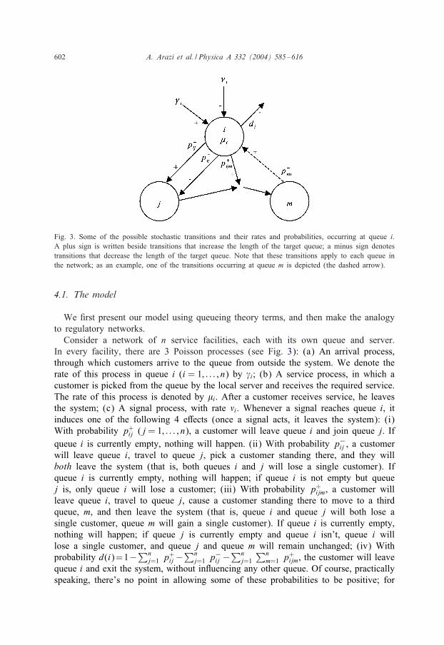
Fig. 3. Some of the possible stochastic transitions and their rates and probabilities, occurring at queue i.A plus sign is written beside transitions that increase the length of the target queue; a minus sign denotestransitions that decrease the length of the target queue. Note that these transitions apply to each queue inthe network; as an example, one of the transitions occurring at queue m is depicted (the dashed arrow).

4.1. The model

We 8rst present our model using queueing theory terms, and then make the analogyto regulatory networks.Consider a network of n service facilities, each with its own queue and server.

In every facility, there are 3 Poisson processes (see Fig. 3): (a) An arrival process,through which customers arrive to the queue from outside the system. We denote therate of this process in queue i (i = 1; : : : ; n) by �i; (b) A service process, in which acustomer is picked from the queue by the local server and receives the required service.The rate of this process is denoted by �i. After a customer receives service, he leavesthe system; (c) A signal process, with rate $i. Whenever a signal reaches queue i, itinduces one of the following 4 e7ects (once a signal acts, it leaves the system): (i)With probability p+

ij (j = 1; : : : ; n), a customer will leave queue i and join queue j. Ifqueue i is currently empty, nothing will happen. (ii) With probability p−

ij , a customerwill leave queue i, travel to queue j, pick a customer standing there, and they willboth leave the system (that is, both queues i and j will lose a single customer). Ifqueue i is currently empty, nothing will happen; if queue i is not empty but queuej is, only queue i will lose a customer; (iii) With probability p+

ijm, a customer willleave queue i, travel to queue j, cause a customer standing there to move to a thirdqueue, m, and then leave the system (that is, queue i and queue j will both lose asingle customer, queue m will gain a single customer). If queue i is currently empty,nothing will happen; if queue j is currently empty and queue i isn’t, queue i willlose a single customer, and queue j and queue m will remain unchanged; (iv) Withprobability d(i)=1−∑n

j=1 p+ij −∑n

j=1 p−ij −

∑nj=1

∑nm=1 p

+ijm, the customer will leave

queue i and exit the system, without inSuencing any other queue. Of course, practicallyspeaking, there’s no point in allowing some of these probabilities to be positive; for


example, having p+ii ¿ 0 for some i implies an event that does not change the state of

the system. However, from a pure mathematical perspective, no such restrictions arerequired.One can see that unlike the case of Jackson networks, here the movement of cus-

tomers between queues does not follow a completion of service, but is rather causedby the arrivals of signals, which act on customers waiting at the queue. The possiblemovements are de8ned by the sets of probabilities {p+

ij}; {p−ij } and {p+

ijm}; thus, it isthese probabilities that characterize the system as a network, with prede8ned connec-tions between its elements.Note that generally, all the mentioned rates and probabilities are allowed to be

any functions of the current state of the network; this, in turn, is de8ned by thevector (k1; k2; : : : ; kn), where ki is the number of customers currently standing at queuei (including the one being served).We can now discuss a possible analogy between this system and a genetic regulatory

network. Each service facility represents a single, speci8c, type of molecule (be it anRNA molecule of some gene, a protein or a small molecule) or gene. The length ofthe queue can be considered to be the number of instances of that molecule type, or, ifthe service facility represents a gene—its expression level. Arrivals of customers fromoutside the system denote a rise in the number of molecules or expression level due tosome external condition change; service, which causes a decrease in the queue length,can be considered as degradation, not related to any other quantity described by themodel apart from the decreased quantity itself. The passage of a customer from queuei to queue j (the 8rst type of signal e7ect) can be thought of as an enhancement ofquantity j by quantity i, at the cost of some work performed by i; for example, if queuei represents the expression level of some gene, then queue j may denote the numberof mRNA molecules transcribed from that gene, and the referred change in quantitieswill represent a transcription of a single mRNA molecule. The loss of a customer inj due to a single arrival in i (the second type of e7ect induced by signals) can belooked at as a repression of i by j. For instance, if the length of queue i is the numberof molecules of some protein, and queue j is the expression level of some gene, thementioned e7ect can represent the repression of the transcription of gene j by protein i.The third type of e7ect—that of i and j teaming together to increase m—can representthe formation of complexes from simpler molecules. The 8nal possibility—that of isimply losing a customer due to the arrival of a signal—can represent a reduction inexpression level or number of molecules due to some external event or condition.Thus, one can use the special case of queueing network presented above, for the

description of a regulatory network, designating directly amounts of molecules or geneexpression levels. The model is able to capture the chemical interactions between theseelements, maintaining their discrete and stochastic nature. Since the rates and probabil-ities can be any function of the state of the whole network, the interactions describedcan be quite complicated (of course, this a7ects the ability to derive analytical resultsfor the model, as discussed below). Interactions which cannot be represented explicitlyby the model, can still be described indirectly, at least to some degree of success. Forexample, the formation of a complex from 3 types of molecules, can be described us-ing an intermediate “queue”, representing the complex formed by 2 of these molecules;


the third molecule will then join the elements of that “queue” (a tight timing of theseevents can be obtained by assigning a relatively high rate to the signals a7ecting theintermediate queue). We note also that the possible events included in the model aresuOcient for the representation, by analogy, of any logical function. This is explainedfurther below.

4.2. Results

In this section we present the results that can be derived when studying a special caseof the model suggested above—namely, when the rates of all the stochastic transitionsinvolved are taken to be constant. Making this assumption allows for the derivation ofseveral results, most notably an explicit expression of the joint probability distributionfunction of the network. We also give formulas for the marginal distributions of eachelement in the network, as well as their average values. Note the similarity of theseresults to those obtained for Jackson networks (see Section 2).Let us start by presenting the notion of aggregate rates of “positive” customers

and “negative” customers arriving to each queue. A “positive” customer arrival is astochastic event that has the e7ect of adding a customer to the queue; a “negative”customer arrival is a stochastic event that has the e7ect of removing a customer fromthe queue (if the queue is not empty). By the word “aggregate” we mean customersarriving to the queue not only from outside the system, but also from other queues, dueto events occurring there. The aggregate arrival rate of “positive” customers in queuei is denoted by +i ; similarly, −i represents the aggregate rate of “negative” customersarriving to that queue.It is possible to prove [44] that if the network reaches a steady state, then there exist

numbers �i; 0¡�i ¡ 1; i=1; : : : ; n, such that the probability of having (simultaneously)k1 customers in the 8rst queue (including the one begin served), k2 customers in thesecond queue, and generally ki customers in the ith queue (i = 1; : : : ; n), is given bythe formula

P(L1 = k1; L2 = k2; : : : ; Ln = kn) =n∏i=1

(1− �i)�kii : (9)

The numbers �i depend on the aggregate rates de8ned above, and obey the equations

�i =+i

�i + −i; i = 1; : : : ; n : (10)

The aggregate rates, in turn, are found by solving the traOc equations of the network:

+i = �i +n∑

j=1

�j$jp+ji +

n∑j=1

n∑m=1

�j�m$jp+jmi ; (11)

−i = $i +n∑

j=1

�j$jp−ji +

n∑j=1

n∑m=1

�j$jp+jim : (12)

To see that these are indeed the aggregate rates, one should keep in mind that here too,as in the Jackson networks, �j is the proportion of time during which queue j is not


empty (we show this below explicitly). Thus, for example, �j$j is the eAective rate inwhich signals arriving to queue j induce some change on the system (remember thata signal arriving to an empty queue has no e7ect), and �j$jp+

ji is the e7ective rate inwhich customers move to queue i from queue j due to signals arriving to queue j.Using similar considerations completes the construction of the aggregate arrival ratesfor each queue.As mentioned previously, the special form of the joint distribution function—a prod-

uct of n factors, each depending on a single queue only—is called product form, and isrelatively common in queueing networks. It allows us to easily derive several featuresregarding each queue separately, without specifying the state of the other queues in thenetwork. For example, the probability that there are ki customers in the ith queue is

P(Li = ki) = (1− �i)�kii : (13)

In particular, the probability of having an empty queue is 1− �i; that is, �i is indeedthe proportion of time during which the ith queue is not empty.Another result readily available, due to the product form, is the average length of

queue i, given by

E(Li) =�i

1− �i: (14)

4.3. Application: Modeling the lac operon

We will now use the suggested model to describe a speci8c, well-studied regulatorycircuit, which is responsible for controlling the expression of the lac operon in E.coli (see, for example, Ref. [26]). The proteins coded for by this operon are requiredfor the transportation and breakdown of lactose. The regulation circuit ensures thatthese proteins will be synthesized only when lactose is present in the cell and a morefavorable carbon source, namely glucose, is absent.More speci8cally, the expression of the lac operon is regulated through a combi-

nation of a positive and a negative transcriptional controls; both are required for ane7ective transcription to occur. The positive regulation is accomplished through theCAP protein, which binds to the DNA near the promoter of the lac operon, and en-hances its transcription considerably. In order for this to occur, CAP must also bindto cyclic AMP molecules; these, in turn, are abundantly found in the cell only whenthe level of glucose is low. Thus, lac is expressed only when glucose levels are low.The negative control is implemented through the lac repressor protein. When present,

this protein binds to an operator on the promoter of the lac operon, and prevents theRNA polymerase from starting the transcription. The presence of lactose causes theremoval of this protein from the DNA, thus enabling the expression of lac.The general model introduced in the previous section is now employed in represent-

ing this mechanism (see Fig. 4). Eight queues are used, designating glucose, lactose,cyclic AMP, CAP (not bound to cyclic AMP), the lac repressor protein, the lac operon,the mRNA produced by it and the synthesized proteins (the lac operon codes for asingle mRNA molecule, which is translated into several proteins; a single queue is usedto represent all of these proteins). We recall that the proposed general model allowed


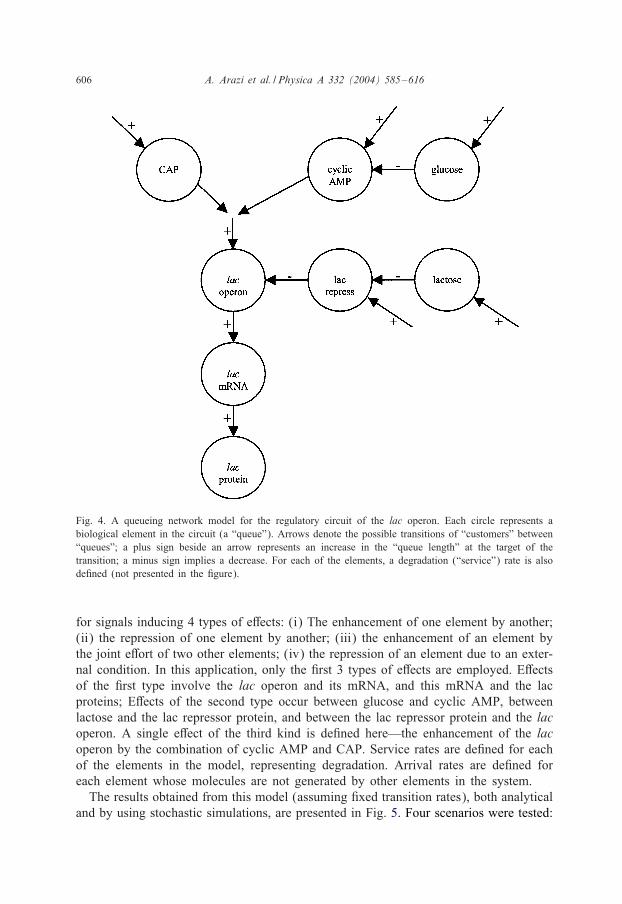
Fig. 4. A queueing network model for the regulatory circuit of the lac operon. Each circle represents abiological element in the circuit (a “queue”). Arrows denote the possible transitions of “customers” between“queues”; a plus sign beside an arrow represents an increase in the “queue length” at the target of thetransition; a minus sign implies a decrease. For each of the elements, a degradation (“service”) rate is alsode8ned (not presented in the 8gure).

for signals inducing 4 types of e7ects: (i) The enhancement of one element by another;(ii) the repression of one element by another; (iii) the enhancement of an element bythe joint e7ort of two other elements; (iv) the repression of an element due to an exter-nal condition. In this application, only the 8rst 3 types of e7ects are employed. E7ectsof the 8rst type involve the lac operon and its mRNA, and this mRNA and the lacproteins; E7ects of the second type occur between glucose and cyclic AMP, betweenlactose and the lac repressor protein, and between the lac repressor protein and the lacoperon. A single e7ect of the third kind is de8ned here—the enhancement of the lacoperon by the combination of cyclic AMP and CAP. Service rates are de8ned for eachof the elements in the model, representing degradation. Arrival rates are de8ned foreach element whose molecules are not generated by other elements in the system.The results obtained from this model (assuming 8xed transition rates), both analytical

and by using stochastic simulations, are presented in Fig. 5. Four scenarios were tested:


(a)

0

0.2

0.4

0.6

0.8(b)

0

2

4

6

8

10

(c)

0

0.2

0.4

0.6

0.8(d)

0

2

4

6

8

10

(e)

0

0.2

0.4

0.6

0.8(f )

0

2

4

6

8

10

(g)

0

0.2

0.4

0.6

0.8

0 2 4 6 8 10 12 14 16 18 20 22 24

(h)

0

2

4

6

8

10

cyclic AMP CAP lacrepr es s or

lac op eron lac mRNA lac proteins

Fig. 5. Results for a model of lac regulation. The graphs to the left depict the distribution of the numberof lac proteins molecules. For the other quantities modeled, only the averages are shown—in the graphs tothe right (the “CAP” bar refers to CAP molecules not bound to cyclic AMP). Note that the rightmost barin thse graphs depicts the average of the distribution shown to the left. The 8gures display both predictedvalues (light shades) and values occurring in stochastic simulations (dark shades). The scenarios presentedin each graph: (a) and (b)—no glucose, no lactose; (c) and (d)—glucose present, lactose absent; (e) and(f)—both glucose and lactose present; (g) and (h)—only lactose present. One can see that indeed, only inthe last scenario the lac proteins are produced in high levels. Note that some of the quantities measureddisplay a rather high variance in their amounts; this can account for the di7erences between predicted andencountered values, and reaOrms the necessity to study statistical properties other than the mere averagesalone.


(i) low glucose level, low lactose level; (ii) high glucose level, low lactose level; (iii)high glucose level, high lactose level and (iv) low glucose level, high lactose level.The levels of glucose and lactose were controlled through the respective arrival rates.As required, the proteins serving for the utilization of lactose were produced in highquantities only in the fourth case.

4.4. Discussion

The main feature of the suggested model is the ability to obtain, for a geneticnetwork of any size and con8guration, the exact distribution function. Analytical resultsregarding arbitrary probabilistic genetic networks are quite rare (in fact, we are familiaronly with Ref. [14]). We haven’t encountered a previous derivation of the explicit jointdistribution function of such a network.On the other hand, these results come at the price of making a quite restricting

assumption—that of 8xed rates. The biological implication of this assumption is thatthe rate in which an element of the regulatory network—for example, some protein—propagates its e7ect on other elements in the network, is independent of its amount;once molecules of this element are present (or, in the case the element is a gene, onceit is active), the rate of its e7ect is constant. Note that this does not mean that theelements in the network function as Boolean components: the larger the amount thereis of a protein, the more time it will induce an e7ect on the network, and the moreenzyme molecules, for example, will be required to turn it o7. This model is 8t todescribe regulation phenomena involving more than two levels of activation; however,the timing of events, as well as their ordering, in some cases, may be erroneous. Thus,such a model should be probably best used in cases where general activity patterns aresought, rather than the exact time evolution of a regulatory system.We note also that the possible chemical interactions included in the model are suf-

8cient for the imitation, by analogy, of any logical function. The repression of oneelement by the other can be thought of as representing a NOT gate; the combinationof two elements for the activation of a third element embodies an AND gate. Recallingresults obtained in the theory of Boolean logic, we conclude that any logical functionis attainable by combining these two elementary operators. Thus, the presented modelpossesses a considerable computational power.The analytical results derived here, most notably the product form solution of the

network, and the methods used for their deduction, are considered to be commonpractice in terms of queueing theory. Thus, by merely adopting the notion that thegenetic network can also be viewed as a queueing network, one can readily earn awealth of imported insights.

5. Queues and dynamic behaviours

As was mentioned in Section 2, most of the research conducted in queueing theoryfocuses on systems that have reached a steady state. Some attention has been given tothe analysis of transient behaviours of queues (see Ref. [45]). However, there is almost


no work dealing with speci8c dynamic behaviours, such as oscillations or chaos (forexamples of the few exceptions, see Refs. [46,47]; note, however, that these di7er fromthe work presented here, both in the modeling scheme and in the analysis methodsapplied).On the other hand, the mathematical 8eld of dynamic systems is well established,

with a vast body of knowledge accumulated over centuries. In addition, it has extensiveapplications in physics, chemistry and biology, as well as other areas of science (see,for example, Refs. [48,49]).These facts come to mind, when one considers the idea that bridging queueing theory

and computational biology may be pro8table to both 8elds. Queueing theory can onlygain, if one is able to import into it some of the insights arising in the study of dynamicsystems in general, and regulatory circuits in particular.One possible way to obtain this is through the Suid approximation of queueing mod-

els. As explained above, this scheme approximates the time evolution of the averagebehaviour of the stochastic system. One can start with a speci8c dynamic, determin-istic, system, and then 8nd a matching stochastic counterpart, such that the averagebehaviour of the latter is approximated by the former. This can be accomplished bycorrectly de8ning the rates of the stochastic transitions, as functions of the system state.We now demonstrate this point. Consider a network of queues, where customers

arrive to service facilities, leave them or move between them due to some stochasticevents, generated by Poisson processes. In each queue, some of these events result inthe arrival of customers to the queue, while others cause the departure of customersfrom the queue. Let us inspect the jth queue. Denote the rates of the former type ofevents (those increasing the length of the queue) by {rj1(L); : : : ; rjR(L)}, and those ofthe latter type by {qj1(L); : : : ; qjQ(L)}, where L = (L1; : : : ; Ln) is the vector of queuelengths, and R and Q are the numbers of rates of each type. That is, the rates areconsidered to be some functions of the state of the system. For the simplicity of thisdemonstration, it is assumed that each arrival or departure changes the queue lengthby a single customer only.Since all the inspected events result from independent Poisson processes, the proba-

bility of each of them to occur during an in8nitesimally short interval of time, (t; t+h],is equal to the product of its rate and h, plus a small quantity o(h) [23]. 3 In addition,up to one event can occur in this interval. Thus, the probability of an arrival of acustomer to the queue during this interval is given by

P+j (L) =

R∑i=1

rji(L)h+ o(h) (15)

and the probability of a departure of a customer from the queue is equal to

P−j (L) =

Q∑i=1

qji(L)h+ o(h) : (16)

3 o(h) is de8ned as being of a smaller order of magnitude than h. That is, when h tends to 0; o(h)=hvanishes.


It follows that the length of the queue at time t + h, given its length at time t, is

Lj(t + h) = Lj(t) + �j(L) ; (17)

where �j is the random variable designating the change in the queue’s length due to anevent occurring in the interval (t; t+ h]. �j can be either 0, −1 or 1, with probabilitiesdepending on P+

j (L) and P−j (L); hence, �j depends indeed on the lengths of the other

queues.It may be desired to estimate the average behaviour of this system. To this end, the

Suid approximation L is presented. This size, which approximates E(L), satis8es theequations

Lj(t + h) = Lj(t) + 1 · P+j (L) + (−1) · P−

j (L) + o(h)

= Lj(t) + h

(R∑i=1

rji(L)−Q∑i=1

qji(L)

)+ o(h) : (18)

Note that this is indeed only an approximation of the time evolution of E(Lj). To seethis, consider the case where one of the rates is given by the product of two queuelengths, Li and Lk . In Eq. (18), this rate will be replaced by Li · Lk , representing itsaverage value; however, it is not generally true that E(Li · Lk) = E(Li) · E(Lk). Thus,this is a mere approximation of the actual average behaviour of E(Lj).Rearranging Eq. (18), dividing by h and taking the limit as h → 0, leads to the next

di7erential equation, approximating the time evolution of the average queue length:

dLjdt

=R∑i=1

rji(L)−Q∑i=1

qji(L) : (19)

Since no constraints are imposed on the functional form of the involved rates (providedthat they all remain positive), the resulting di7erential equation can take a wide rangeof possible forms. Thus, an abundance of types of complex dynamic behaviours canbe integrated into the queueing network.In the analysis conducted here, it is desired to inspect the e7ect of the workload in

the system on the divergence from the approximated average behaviour. Alternatively,one can consider the e7ect of the size of a change induced by a single stochasticevent. Instead of assuming that each arrival increments the queue length by 1, and eachdeparture decrements it by 1, we will set these changes to be ±). By varying the sizeof ), it is now possible to study the approximated average behaviour of the queueingsystem at di7erent orders of magnitude of workloads. This leads to the followingequation:

dLjdt

= )

[R∑i=1

rji(L)−Q∑i=1

qji(L)

]: (20)

The multiplication by ) implies a mere scaling of the time axis; thus, the approximatedaverage behaviour itself does not qualitatively change—only the time it takes for itsmanifestation. However, the divergence of the actual behaviour from this approximatedaverage does depend on ).


The immediate bene8t from such an analysis is the ability to recognize the localtransition rates required to produce a desired system-wise behaviour, and by this gain,maybe, a more general insight regarding the relation between local interactions andglobal dynamics, in the context of queues. However, one needs not settle for this: thefull strength of dynamic systems theory can be made available for the exploration ofqueueing systems, allowing for the utilization of such tools as phase space investiga-tion, stability analysis, bifurcation analysis, and so on. Moreover, using tools developedin the study of the approximation schemes of stochastic models, it is possible to es-tablish further results concerning the behaviour of stochastic queueing systems, suchas the dispersion around the approximated average trajectory, the distribution of theperiod time (if the matching dynamic system displays cycles), the distribution of theduration of time such a system stays in one steady state before jumping to another (ifmultistability exists), and so forth.An example of such a work, done in relation to a biochemical system, can be found

in Ref. [15] (mentioned in Section 3). The authors there started with a set of di7erentialequations, generating an oscillatory behaviour, which can be regarded as a simpli8edmodel of circadian oscillations. They then presented a stochastic model, describing thesame biological sizes, and de8ned the transition rates in it so that indeed, its averagebehaviour can be approximated by the oscillations predicted by the deterministic model.They derived results similar to those suggested above. In particular, they discussed thevalidity of the Suid approximation, as a function of the system’s size: the larger thesystem is, the more closer its behaviour to that of its deterministic counterpart.Here we suggest to perform a similar analysis, but to further interpret the functional

form of the transition rates in terms relevant to queueing systems. This is demonstratedin the following example.Consider the next set of di7erential equations, consisting of the well-known Brusse-

lator model, studied in chemistry [50]:dXdt

= A− (B+ 1)X + X 2Y ;

dYdt

= BX − X 2Y : (21)

These equations describe the next (hypothetical) chemical reactions:

A → X ;

B+ X → Y + D ;

2X + Y → 3X ;

X → E :

We can now consider a speci8c queueing network (a Jackson network with varyingrates, as it is), whose average behaviour can be approximated by the dynamics ofthe Brusselator model. The network will consist of two queues. The length of the8rst queue matches X , while the length of the second queue coincides with Y . Therespective Suid approximations are denoted by X and Y . Denote the external arrivalrates to the queues by �1 and �2, and the service rates by �1 and �2. Let p1;2 be the


probability that a customer completing service in the 8rst queue moves to the secondqueue, and d1 =1−p1;2 the probability that the customer leaves the system. Similarly,de8ne p2;1 and d2.We now follow the procedure outlined above. The analysis here is limited to the

case where both queues are not empty. Since, in order for the presented approximationto be valid, it is assumed that the system is overloaded (that is, ) is close to 0), thisis the common state of the network. However, to complete the picture presented here,the cases where at least one of the queues is empty should be investigated as well.Consider the 8rst queue. The stochastic events resulting in the increment of the length

of this queue are the arrival of a customer from outside the system, with rate �1, and thecompletion of service in the second queue, provided that the served customer moves tothe 8rst queue; the rate of this event is given by the product �2p2;1 (there is no needto further multiply this size by the proportion of time during which the second queueis not empty, since, as stated above, we assume that both queues currently containcustomers). A loss of a customer in the queue is caused solely by a completion ofservice, with rate �1. Hence, the resulting di7erential equation is

dXdt

= )[(�1 + �2p2;1)− �1] : (22)

A similar analysis of the second queue produces the equation

dYdt

= )[(�2 + �1p1;2)− �2] : (23)

In these equations, the rates are written in terms of X and Y , instead of X and Y .Comparing these equations to the Brusselator equations, one can see that the followingchoice of parameters results in an identical set of equations (up to a multiplicationby )):

�1 = A; �2 = 0

�1 = (B+ 1)X; �2 = X 2Y

p1;2 =B

B+ 1; p2;1 = 1

d1 =1

B+ 1; d2 = 0

That is, customers reach the system from the outside at a constant rate, A, and jointhe 8rst queue (the second queue does not have an external inSow of customers).These customers are served in a rate equal to (B+1)X . After his service is completed,a customer leaves the system with probability 1=(B + 1), or joins the second queuewith probability B=(B + 1). The service rate in the second queue is given by X 2Y . Acustomer served in the second queue, returns to the 8rst queue with probability 1. Thisscenario is depicted in Fig. 6.As mentioned above, the distance of the actual behaviour from this approximated

average depends on the workload in the system or, equivalently, on the size of thechange induced by a single stochastic transition, ): the smaller the change, the moreregular the global behaviour of the system. This is demonstrated in Fig. 7, displaying


1 XL =1

XB )1(1 +=µ

2 YL =2

YX 2

2 =µ

A

1

1

+B

1+B

B

1

Fig. 6. A Jackson network displaying, approximately, an average behaviour of oscillations. Each circlerepresents a single queue. Customers arrive from the outside to queue 1 only, at a constant rate A. Theservice rates are written inside the circles; transition probabilities appear next to the arrows.

examples of actual trajectories produced by this network, for di7erent sizes of ). Theresulting queueing system exhibits, roughly, a periodic behaviour, rarely encounteredin queueing theory models and studies.We will now suggest an interpretation to the functional form of the rates appearing in

this model, focusing our attention on the rates which can be considered to be “peculiar”,in queueing theory terms—the service rates. The linear service rate in the 8rst queueposes the lesser problem, since such rates do occur in queues: when a service facilityhas an in8nite number of servers (or, more realistically, a number of servers which ispractically larger than any number of waiting customers), the total service rate in thefacility increases by a constant value (representing the service rate of a single server)with every new customer joining the system. So, explaining the form of this rate doesnot require us to employ unorthodox ideas.The service rate of the second queue, however, is a di7erent story. Here it follows

that the longer the 8rst queue is, the more eOcient is the server in the second facility.To explain this odd situation, we suggest the notion of customers acting as servers:customers waiting in the 8rst queue participate, in the meantime, in the service ofcustomers standing in the second queue, enhancing the rate of service there. The factthat this rate increases with X 2, rather than X , implies that this enhancement of serviceresults from connections, or a cooperation, forming between pairs of customers standingin the 8rst queue; the “computation” performed by the “network” of these customers isdone by its “edges”, rather than its “nodes”. This scheme of computation is similar tothe one encountered in neural networks. To complete the picture, the linear dependenceon Y of this rate suggests that a large number of servers are present in the secondfacility as well, and that these servers are responsible for the utilization of customerswaiting in the 8rst queue.The idea of waiting customers, which in the meantime supply some sort of service,

is not so farfetched as it may 8rst seem. In fact, such a scheme already exists forsome time: by this, we refer to the SETI@home project, managed by the Space Sci-ences Laboratory at the University of California, Berkeley. This venture, which aims atsearching for extraterrestrial intelligence, utilizes idle personal computers, connected tothe Internet, using their computational power to process its data (recordings made by


Fig. 7. The occurrence of periodic behaviour in queueing networks. The queueing network de8ned in the textwas simulated, using di7erent sizes of ), the size of a change induced by a single transition. The 8gures onthe left column depict trajectories in the phase space of the system, in which the horizontal axis designatesthe length of the 8rst queue (X ) and the vertical axis the length of the second queue (Y ); the 8gures onthe right column show the change in time in the length of each queue (the 8rst queue is shown in darkshades, the second in light shades). (a) and (b) describe the deterministic system, which approximates theaverage behaviour of the queueing network. The other Figures correspond to di7erent sizes of ): in (c) and(d), )=0:01; in (e) and (f), )=0:05; and in (g) and (h), )=0:1. As can be seen, the larger ) is, the furtherthe system deviates from its approximated average behaviour. Notice that changing ) also scales the timeaxis.

radio telescopes). This is accomplished using a designated screen saver, installed onthe participating PCs: when such a computer is waiting for user input long enough, thisscreen saver is activated, and the processing of SETI data takes place. Hence, the PCwaiting for user response can be viewed as a customer waiting on a queue, supplyingsome service in the meantime.Generally speaking, researching queueing networks which display complex dynamic

behaviours will usually involve transitions rates depending on various componentsof the system, and in particular, the lengths of other queues in the network. Such


dependencies can be expected to have nontrivial, nonlinear forms. Thus, notions suchas customers supplying service, or networks of customers performing some computa-tion, will probably be recurring themes in such models. To these one must add therequest that the queueing network is overloaded, so that the Suid approximation canbe considered to be valid.

6. Conclusions

It is becoming increasingly acknowledged that genetic regulatory systems have dis-crete and stochastic aspects to their behaviour, and should be modeled accordingly.Thus, the study of these systems can bene8t from the integration of knowledgeacquired in existing disciplines, which specialize in modeling systems displaying suchaspects. Queueing theory is an example of such a discipline.We have demonstrated here the application of modeling and analysis techniques,

borrowed from queueing theory, to the description of an arbitrary genetic network.This allowed for the derivation of the probability distribution function of the network.It should be clear, however, that there is more to accomplish from the interaction of thetwo disciplines. Queueing theory literature is extensive and diverse, and further delvinginto it, while still keeping in mind the biological problems at hand, can probably yieldseveral other useful results.In addition, we have suggested that queueing theory may bene8t as well from this

interdisciplinary dialogue. The employment of methodologies and insights gained in thestudy of dynamical systems in general, and the dynamics of genetic regulatory networksin particular, can promote the integration of complex behaviours into queueing models,enriching and diversifying the existing results.

Acknowledgements

The authors would like to thank Zeev Schuss for his helpful comments in preparingthis paper. We would also like to thank Hila Rosenberg, for the illustration appearing inFig. 1. E.B.J. would like to thank Mark Ptashne, for insightful conversations regardinggenetic networks.

References

[1] F.R. Blattner, Science 277 (1997) 1453.[2] S.T. Cole, Nature 393 (1998) 537.[3] The C. Elegans Sequencing Consortium, Science 282 (1998) 2012.[4] F.S. Collins, A. Patrinos, E. Jordan, A. Chakravati, R. Gesteland, L. Walters, Science 282 (1998) 682.[5] M. Ptashne, A. Gann, Genes & Signals, Cold Spring Harbor Laboratory Press, New York, 2002.[6] H. De Jong, J. Comput. Biol. 9 (2002) 67.[7] P. Smolen, D.A. Baxter, J.H. Byrne, Bull. Math. Biol. 62 (2000) 247.[8] H.H. McAdams, A. Arkin, Annu. Rev. Biophys. Bimol. Struct. 27 (1998) 199.[9] B.C. Goodwin, Temporal Organization in Cells, Academic Press, New York, 1963.


[10] S.A. Kau7man, J. Theor. Biol. 22 (1969) 437.[11] A. Arkin, J. Ross, H.H. McAdams, Genetics 149 (1998) 1633.[12] T.B. Kepler, T.C. Elston, Biophys. J. 81 (2001) 3116.[13] J. Peccoud, B. Ycart, Theor. Popul. Biol. 48 (1995) 222.[14] M. Thattai, A. van Oudenaarden, Proc. Natl. Acad. Sci. USA 98 (2001) 8614.[15] D. Gonze, J. Halloy, P. Gaspard, J. Chem. Phys. 116 (2002) 10 997.[16] L. Kleinrock, Queueing System, Vol. 1, John Wiley & Sons, New York, 1975.[17] T.G. Robertazzi, Computer Networks and Systems: Queueing Theory and Performance Evaluation,

Springer, New York, 1990.[18] E. Gelenbe, J. Appl. Probab. 28 (1991) 656.[19] J.R. Artalejo, Eur. J. Oper. Res. 126 (2000) 233.[20] E. Gelenbe, Lect. Notes Comput. Sci. 2459 (2002) 1.[21] E. Gelenbe, Neural Comput. 1 (1989) 502.[22] H. Bakircioglu, T. Kocak, Eur. J. Oper. Res. 126 (2000) 319.[23] W. Feller, An Introduction to Probability Theory and its Application, Wiley, New York, 1968.[24] H.A. Kramers, Physica 7 (1940) 284.[25] J.E. Moyal, J. Roy. Stat. Soc. 11 (1949) 150.[26] B. Alberts, D. Bray, J. Lewis, M. Ra7, K. Roberts, J.D. Watson, Molecular Biology of the Cell, 3rd

Edition, Garland Publishing, New York, 1994.[27] R. Milo, S. Shen-Orr, S. Itzkovitz, N. Kashtan, D. Chklovskii, U. Alon, Science 298 (2002) 824.[28] N. Friedman, M. Linial, I. Nachman, D. Pe’er, J. Comput. Biol. 7 (2000) 601.[29] S.A. Kau7man, Sci. Am. 265 (1991) 78.[30] S.A. Kau7man, The Origins of Order: Self-Organization and Selection in Evolution, Oxford University

Press, New York, 1993.[31] R. Somogyi, C.A. Sniegoski, Complexity 1 (1996) 45.[32] Z. Szallasi, S. Liang, in: R.B. Altman, A.K. Dunker, L. Hunter, T.E. Klein (Eds.), Proceedings of the

Paci8c Symposium on Biocomputing (PSB’98), Vol. 3, World Scienti8c Publishing, Singapore, 1998,pp. 66–76.

[33] G. Weisbuch, J. Theor. Biol. 121 (1996) 255.[34] S. Liang, S. Fuhrman, R. Somogyi, in: R.B. Altman, A.K. Dunker, L. Hunter, T.E. Klein (Eds.),

Proceedings of Paci8c Symposium on Biocomputing (PSB’98), Vol. 3, World Scienti8c Publishing,Singapore, 1998, pp. 66–76.

[35] T. Akutsu, S. Miyano, S. Kuhara, Bioinformatics 16 (2000) 727.[36] I. Shmulevich, E.R. Dougherty, S. Kim, W. Zhang, Bioinformatics 18 (2002) 261.[37] H.H. McAdams, A. Arkin, Trends Genet. 15 (1999) 65.[38] D.T. Gillespie, J. Phys. Chem. 81 (1977) 2340.[39] M.A. Gibson, J. Bruck, J. Phys. Chem. A 104 (2000) 1876.[40] R. Thomas, J. Theor. Biol. 153 (1991) 1.[41] D.T. Gillespie, J. Chem. Phys. 113 (2000) 297.[42] H. McAdams, L. Shapiro, Science 269 (1995) 650.[43] E. Gelenbe, J. Appl. Probab. 30 (1993) 742.[44] A. Arazi, M.Sc. Dissertation, Tel-Aviv University, 2003.[45] H. Chen, D.D. Yao, Fundamentals of Queueing Networks, Springer, Berlin, 2001.[46] C. Chase, J. Serrano, P.J. Ramadge, IEEE Trans. Automat. Control 38 (1993) 70.[47] C.M. Rump, S. Stidham Jr., Manage Sci. 44 (1998) 246.[48] J.M.T. Thompson, H.B. Stewart, Nonlinear Dynamics and Chaos, Wiley, New York, 1986.[49] H. Haken, Synergetics, Springer, Berlin, 1977.[50] G. Nicolis, I. Prigogine, Self-Organization in Non-Equilibrium Systems. From Dissipative Structures to

Order Through Fluctuations, Wiley, New York, 1977.

Documents

Bridging genetic networks and queueing theory - TAUuriy/Papers/Bridging-genetic-networks-and... · A. Arazi et al./Physica A 332 (2004) 585–616 587 The tools suppliedby queueing