Bloch equations �

Ravinder Reddy�

Outline��•  Magnetic moment and Larmor precession �•  Bloch equations�

– With and without relaxation �– With RF and Relaxation �–  Transformation into rotating frame�–  Steady state solutions�

•  Absorption and dispersion �–  Steady state solutions�–  Pulse responses�

•  Advantages and Limitations of BE �–  Single pulse and spin-echo sequence�

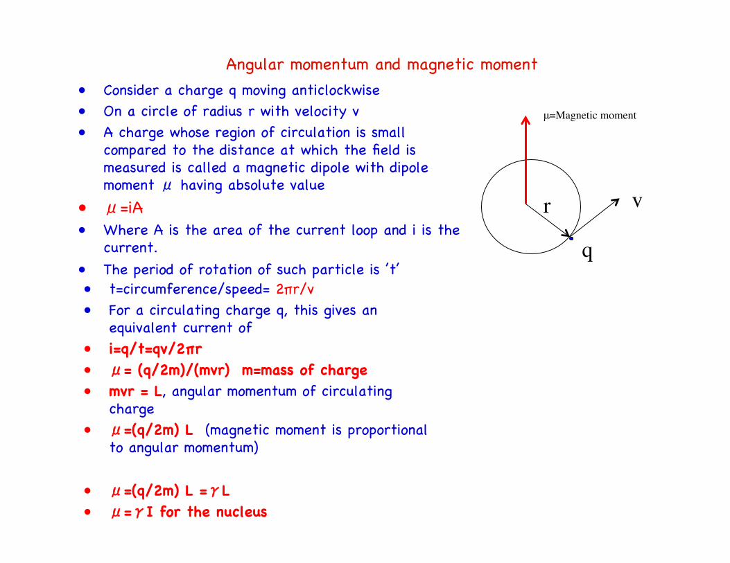
Angular momentum and magnetic moment �•  Consider a charge q moving anticlockwise�•  On a circle of radius r with velocity v �•  A charge whose region of circulation is small

compared to the distance at which the field is measured is called a magnetic dipole with dipole moment μ having absolute value�

•  μ=iA �•  Where A is the area of the current loop and i is the

current. �•  The period of rotation of such particle is ’t’�

�

μ=Magnetic moment

v r

q •  t=circumference/speed= 2πr/v �•  For a circulating charge q, this gives an

equivalent current of�•  i=q/t=qv/2πr�•  μ= (q/2m)/(mvr) m=mass of charge �•  mvr = L, angular momentum of circulating

charge�•  μ=(q/2m) L (magnetic moment is proportional

to angular momentum)�

•  μ=(q/2m) L =γL �•  μ=γI for the nucleus�

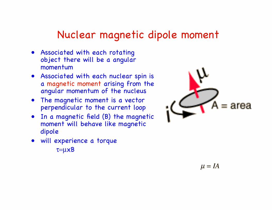
Nuclear magnetic dipole moment �•  Associated with each rotating

object there will be a angular momentum�

•  Associated with each nuclear spin is a magnetic moment arising from the angular momentum of the nucleus�

•  The magnetic moment is a vector perpendicular to the current loop �

•  In a magnetic field (B) the magnetic moment will behave like magnetic dipole�

•  will experience a torque� τ=µxB �

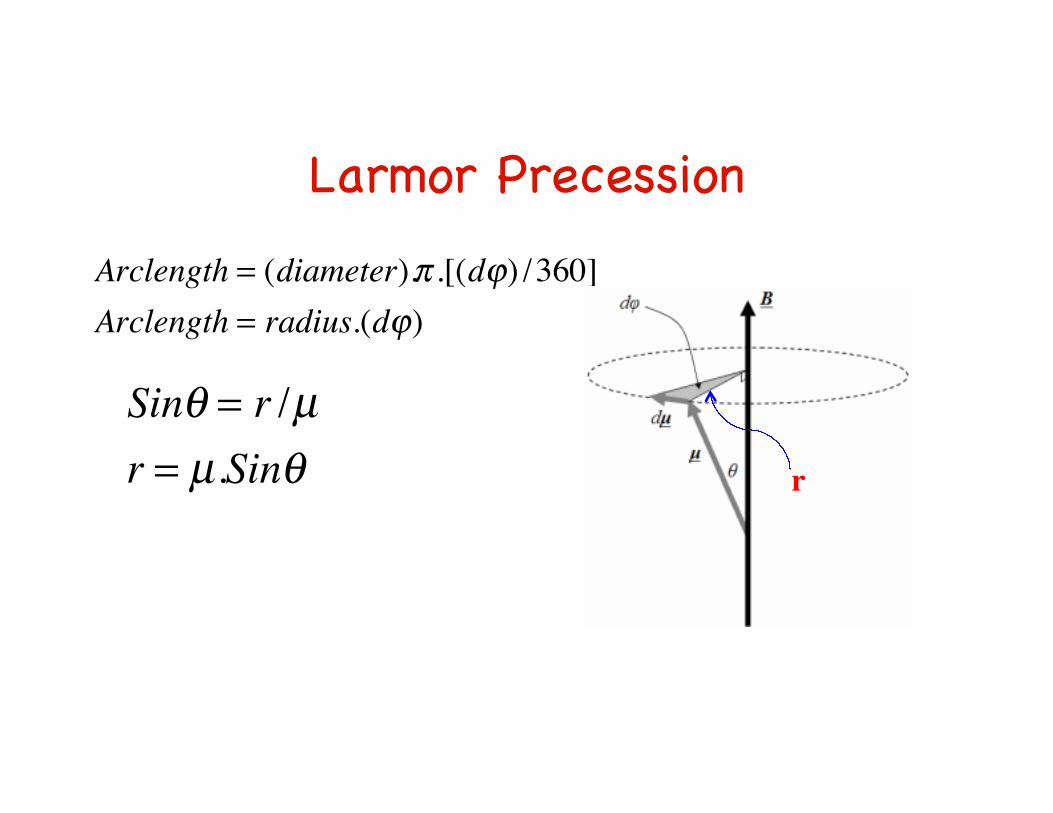
Larmor Precession �

�

Arclength = (diameter).π .[(dϕ) /360]Arclength = radius.(dϕ)

�

Sinθ = r /µr = µ.Sinθ r

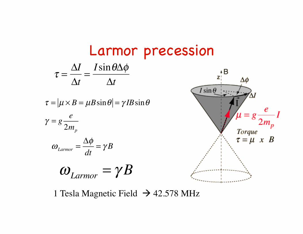
Larmor precession �

�

τ =ΔIΔt

=I sinθΔφ

Δt

1 Tesla Magnetic Field à 42.578 MHz

ω Larmor = γ B

τ = µ × B = µBsinθ = γ IBsinθ

γ = g e2mp

ω Larmor =Δφdt

= γ B

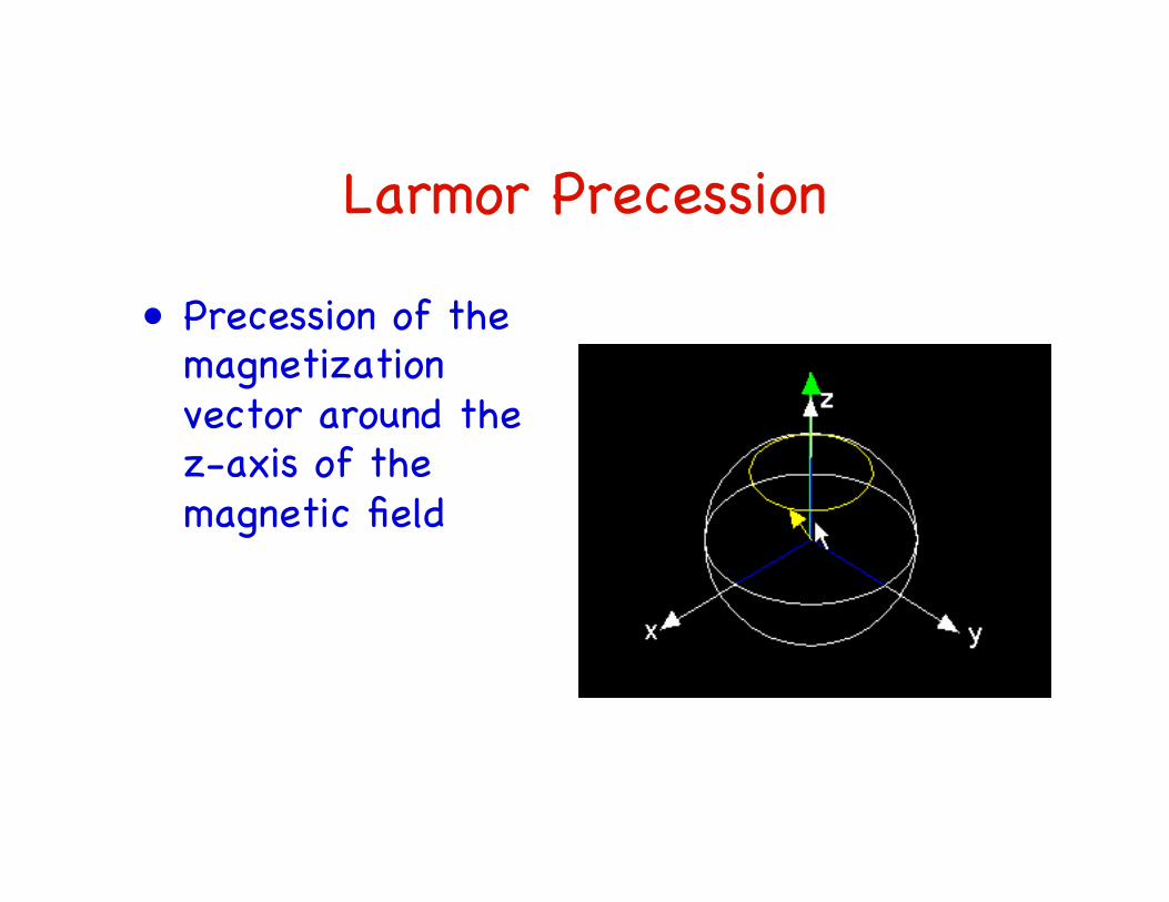
Larmor Precession �

•  Precession of the magnetization vector around the z-axis of the magnetic field �

Boltzman factor�

•  Boltzman factor�•  b=(N+-N-)/N=ΔE/2kT �•  K=1.3805x10-23 J/Kelvin �

•  T=300 k �•  ΔE= hν=6.626x10-34 Js x100 MHz �•  b= 7.99 x10-6�

•  How is the Boltzman factor changes with Bo and or T?�

Bloch equations�

•  In terms of total angular momentum of a sample�

�

dΜdt

= γΜxB

�

M= µi

i

∑

•  Total magnetic moment of a sample�

•  Interaction of magnetic moment with magnetic field gives a torque on the system and changes the angular momentum of the system�

�

M = γL

�

τ =dL

dt= M × B

�

dMdt

= γdLdt

= γM × B

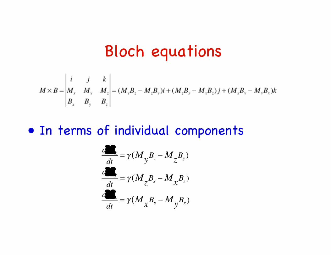
Bloch equations�

•  In terms of individual components�dΜx

dt= γ (MyBz −MzBy )

dΜy

dt= γ (MzBx −MxBz )

dΜz

dt= γ (MxBy −MyBx )

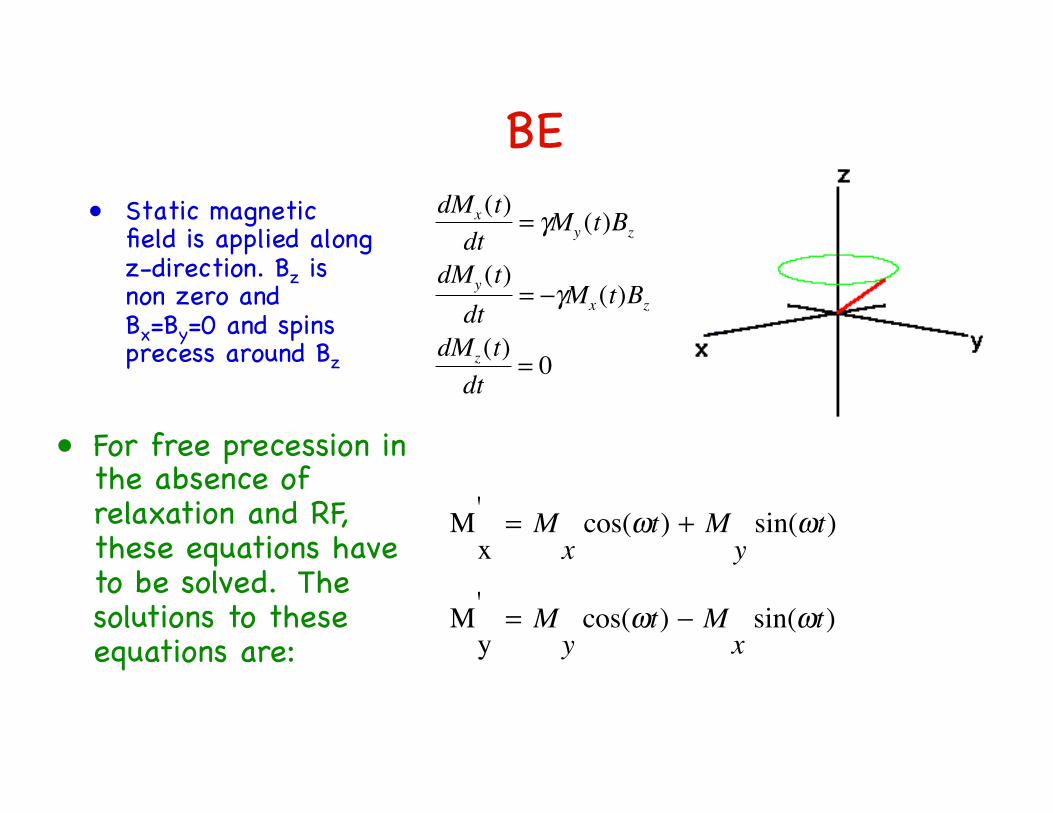
BE�•  Static magnetic

field is applied along z-direction. Bz is non zero and Bx=By=0 and spins precess around Bz�

•  For free precession in the absence of relaxation and RF, these equations have to be solved. The solutions to these equations are: �

�

Mx

'= M

xcos(ωt) + M

ysin(ωt)

My

'= M

ycos(ωt) − M

xsin(ωt)

�

dMx (t)dt

= γMy (t)Bz

dMy (t)dt

= −γMx (t)Bz

dMz(t)dt

= 0

Including relaxation �•  Spin-lattice and spin-

spin relaxation can be treated as first order processes with characteristic times T1 and T2 respectively. �

�

dMx

dt= γ (M

yBz−M

zBy) −Mx

T2

dM y

dt= γ (M

zBx−M

xBz) −

My

T2

dMz

dt= γ (M

xBy −My

Bx ) − −(M

z−M

o)

T1

•  Including relaxation terms alone and treating that the Bo applied along z-axis (Bx=By=0, Bo=Bz)) the Bloch equations are given by: �

�

�

dMx

dt= γM

yBo−Mx

T2

dMy

dt= −γM

xBo−

My

T2

dMz

dt= −(M

z−M

o)

T1

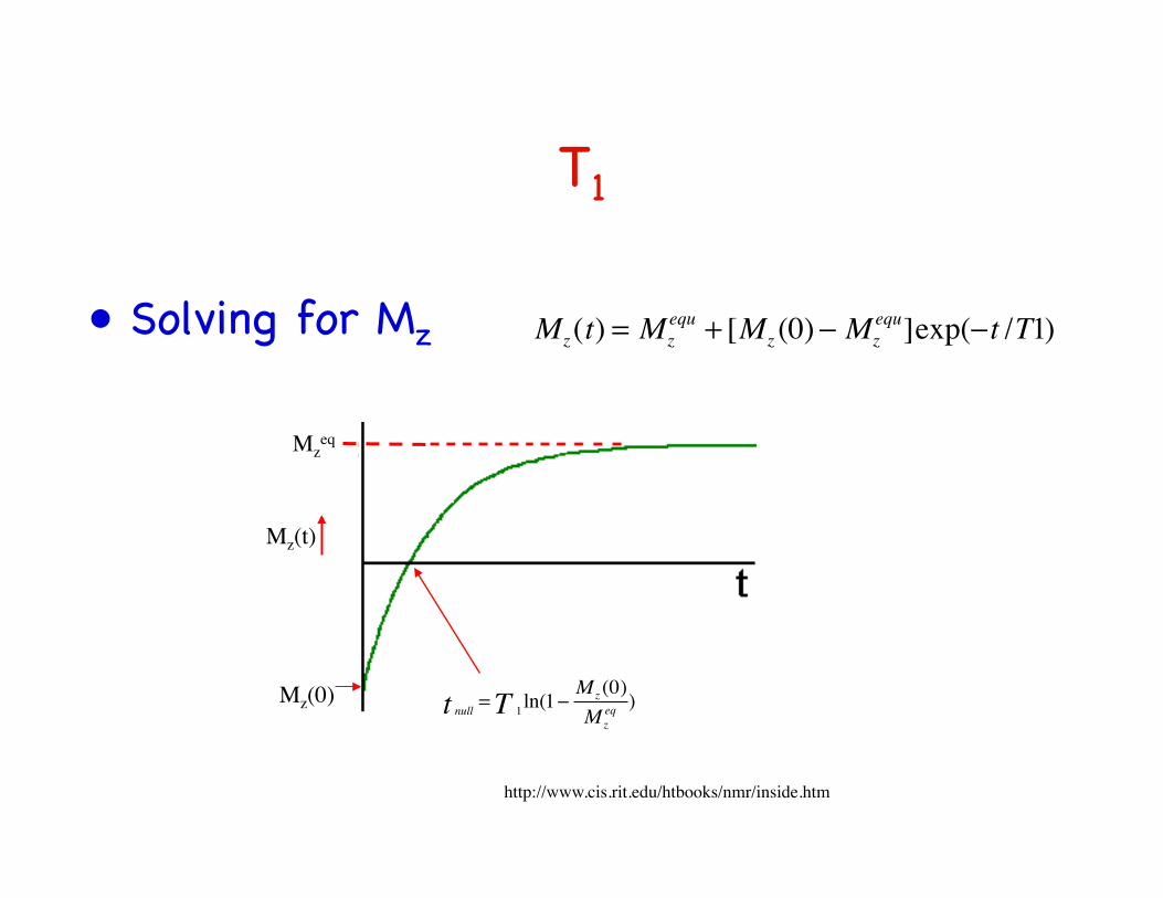
T1 �

•  Solving for Mz�

�

Mz(t) = Mz

equ+ [Mz (0)− Mz

equ]exp(−t /T1)

Mz(t)

Mz(0) nullt = 1T ln(1−

Mz (0)Mz

eq )

Mzeq

http://www.cis.rit.edu/htbooks/nmr/inside.htm

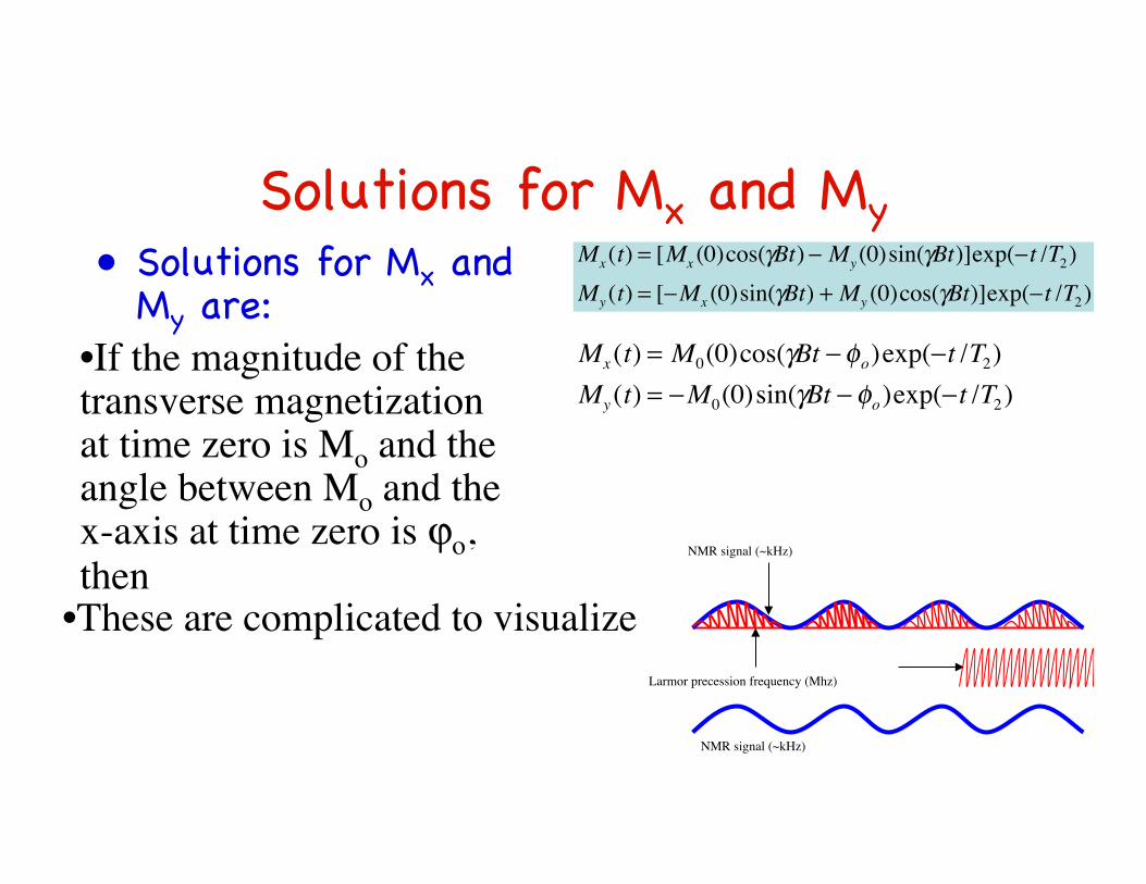
Solutions for Mx and My�•  Solutions for Mx and

My are: �

�

Mx(t) = [M

x(0)cos(γBt) − M

y(0)sin(γBt)]exp(−t /T2)

My (t) = [−Mx (0)sin(γBt) + My (0)cos(γBt)]exp(−t /T2)

�

Mx (t) = M0(0)cos(γBt −φo)exp(−t /T2)

My (t) = −M0(0)sin(γBt − φo)exp(−t /T2)

• These are complicated to visualize

• If the magnitude of the transverse magnetization at time zero is Mo and the angle between Mo and the x-axis at time zero is ϕo, then

NMR signal (~kHz)

Larmor precession frequency (Mhz)

NMR signal (~kHz)

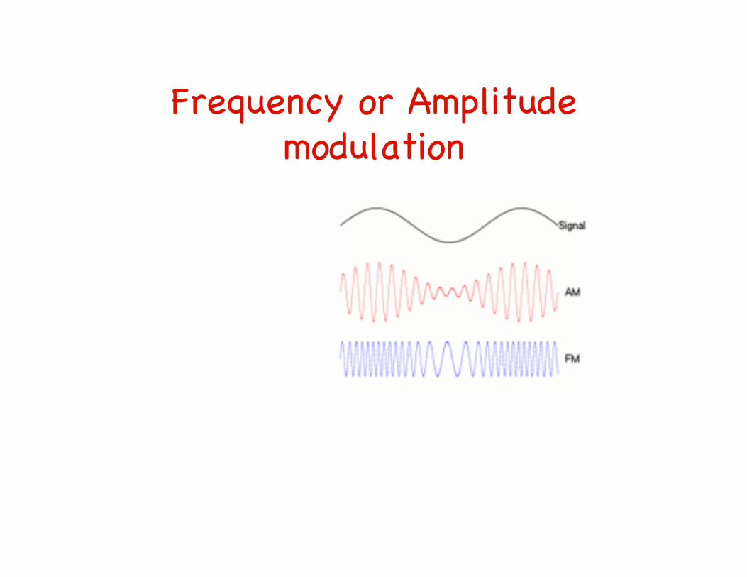
Frequency or Amplitude modulation �

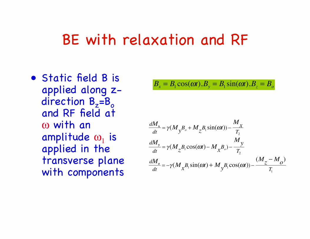
BE with relaxation and RF�

•  Static field B is applied along z-direction Bz=Bo and RF field at ω with an amplitude ω1 is applied in the transverse plane with components�

�

Bx = B1 cos(ωt),By = B1 sin(ωt),Bz = Bo

�

dMx

dt= γ (M

yBo

+ MzB1sin(ωt)) −

Mx

T2

dM y

dt= γ (M

zB1cos(ωt)−M

xBo) −

My

T2

dMz

dt= −γ (M

xB1 sin(ωt)+ M

yB1 cos(ωt))−

(Mz−M

o)

T1

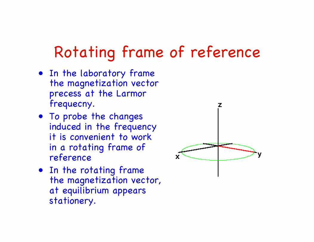
Rotating frame of reference�•  In the laboratory frame

the magnetization vector precess at the Larmor frequecny.�

•  To probe the changes induced in the frequency it is convenient to work in a rotating frame of reference�

•  In the rotating frame the magnetization vector, at equilibrium appears stationery.�

Magnetization vector�•  Bo is along z-axis �•  Equilibrium

magnetization Mo is along z-axis�

•  Mx and My = 0�

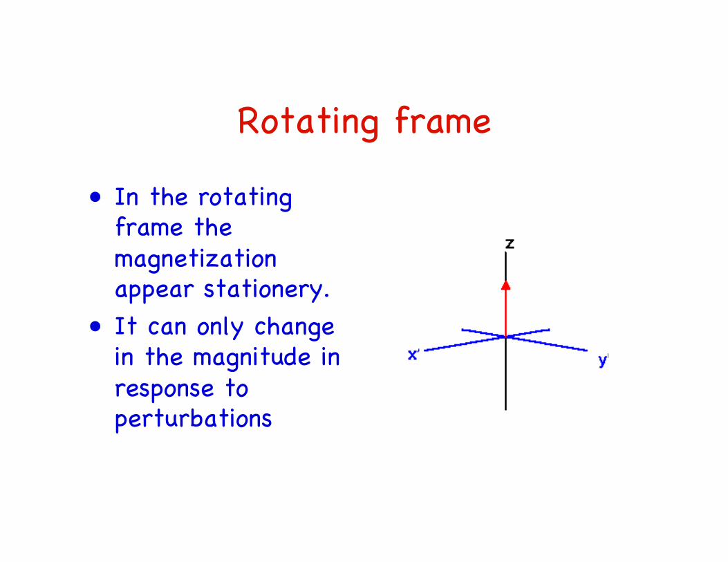
Rotating frame �

•  In the rotating frame the magnetization appear stationery.�

•  It can only change in the magnitude in response to perturbations�

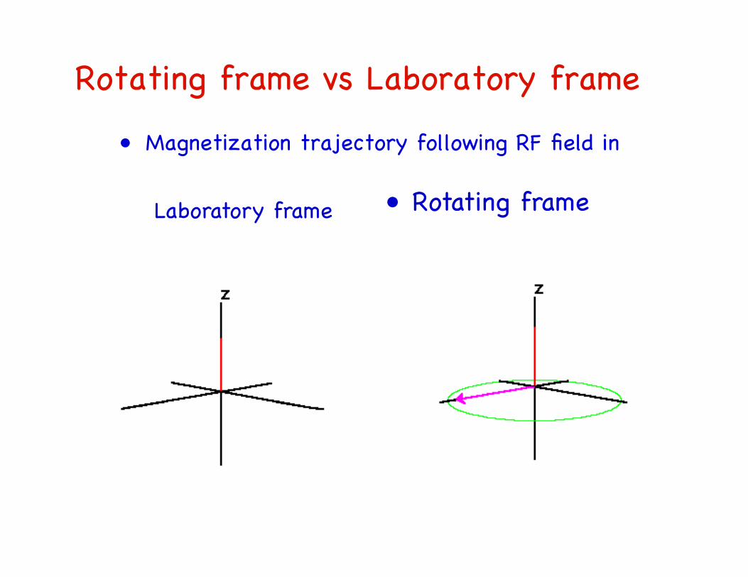
Rotating frame vs Laboratory frame�•  Magnetization trajectory following RF field in �

•  Rotating frame�Laboratory frame�

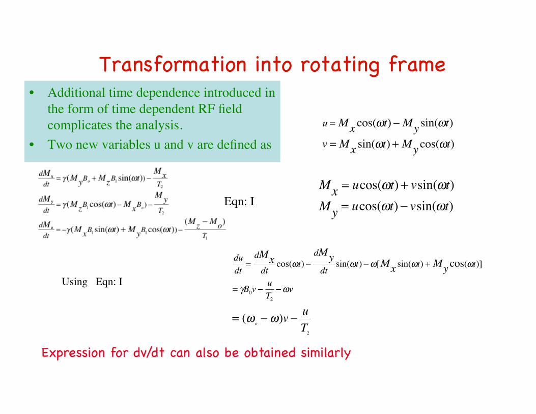
Transformation into rotating frame�•  Additional time dependence introduced in

the form of time dependent RF field complicates the analysis.

•  Two new variables u and v are defined as

�

u = Mxcos(ωt)−M

ysin(ωt)

v = Mxsin(ωt)+ M

ycos(ωt)

�

Mx

= ucos(ωt)+ vsin(ωt)

My

= ucos(ωt)− vsin(ωt)

�

= (ωo− ω)v −

u

T2

Expression for dv/dt can also be obtained similarly �

du

dt=

dMx

dtcos(ωt) −

dMy

dtsin(ωt) −ω[M

xsin(ωt) + M

ycos(ωt)]

= γB0v −

u

T2

−ωvUsing Eqn: I

Eqn: I

Rotating frame solutions�

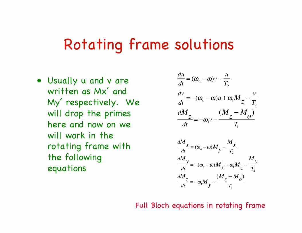
•  Usually u and v are written as Mx’ and My’ respectively. We will drop the primes here and now on we will work in the rotating frame with the following equations�

�

du

dt= (ω

o−ω)v −

u

T2

dv

dt= −(ω

o−ω)u + ω1Mz

−v

T2

dMz

dt= −ω1v −

(Mz−M

o)

T1

�

dMx

dt= (ω

o−ω)M

y−

Mx

T2

dMy

dt= −(ω

o−ω)M

x+ ω

1Mz−

My

T2

dMz

dt= −ω1My

−

(Mz−M

o)

T1

Full Bloch equations in rotating frame�

Steady state solutions�

•  If we assume that the system has been allowed to soak in this combination of of static and time varying fields a steady state ultimately will be reached in which none of the components change with time: � �

δω = (ωo−ω)

ω1 = γB1

• now on we will work in the rotating frame with the following eqautions�

�

Mx =ω1T22δω

1+ ω12T1T2

+ (T2δω)2

Mo

My =ω1T2

1+ ω12T1T2

+ (T2δω)2

Mo

Mz =1+T

22δω2

1+ ω12T1T2

+ (T2δω)2

Mo

(ωo −ω )My −MxT2

= 0

−(ωo −ω )Mx +ω1Mz −MyT2

= 0

−ω1My −(Mz −Mo)

T1= 0

Steady state solutions in the limiting case�

•  In the limiting case of small RF limit,

�

�

ω1

2T1T2

<< 1

�

Mx≈ (ω

1Mo)

T2

2δω

1+ (T2δω)

2= ω

1MoG(δω)

My≈ (ω1Mo

)T2

1+ (T2δω)

2= ω1Mo

F(δω)

•  The functional forms F and G are the absorption and dispersion for a particular kind of line known as a Lorentzian line.

�

�

G(δω) =

T2

2δω

1+ (T2δω )

2

F(δω) =

T2

1+ (T2δω )

2

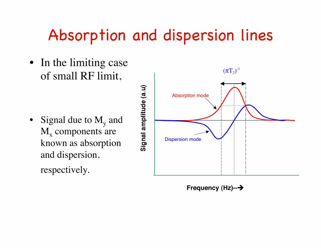
Absorption and dispersion lines�•  In the limiting case

of small RF limit, �

•  Signal due to My and Mx components are known as absorption and dispersion, respectively. �

(πT2)-1

Frequency (Hz)--

Absorption mode

Dispersion mode

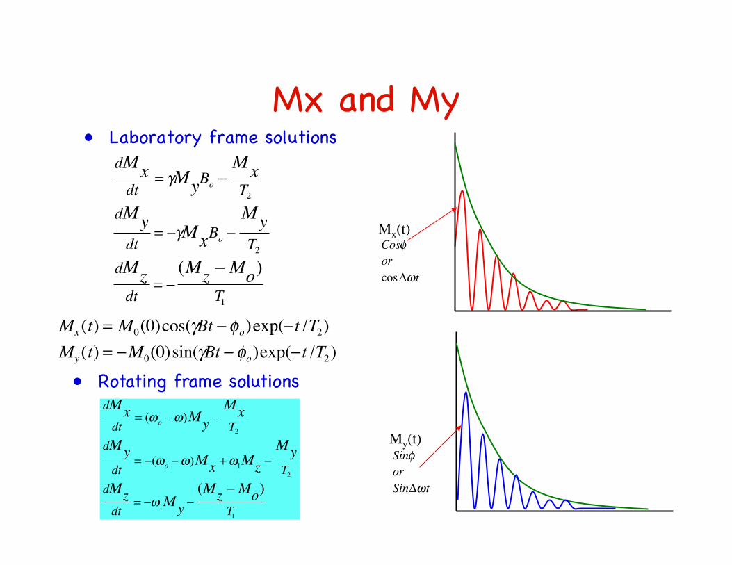
Mx and My�•  Laboratory frame solutions�

�

dMx

dt= γM

yBo−Mx

T2

dMy

dt= −γM

xBo−

My

T2

dMz

dt= −(M

z−M

o)

T1

�

dMx

dt= (ω

o−ω)M

y−

Mx

T2

dMy

dt= −(ω

o−ω)M

x+ ω

1Mz−

My

T2

dMz

dt= −ω1My

−

(Mz−M

o)

T1

•  Rotating frame solutions�

�

Mx (t) = M0(0)cos(γBt −φo)exp(−t /T2)

My (t) = −M0(0)sin(γBt − φo)exp(−t /T2)

Mx(t) CosφorcosΔωt

My(t) SinφorSinΔωt

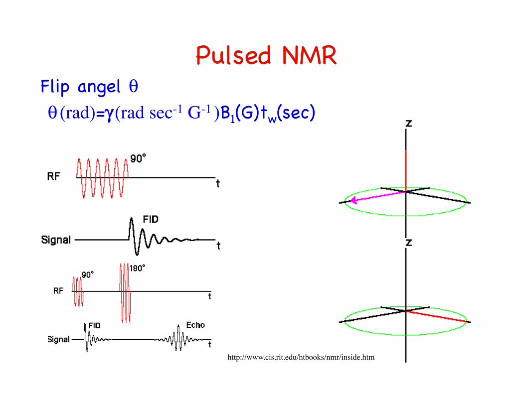
Pulsed NMR �Flip angel θ θ (rad)=γ (rad sec-1 G-1 )B1(G)tw(sec)�

http://www.cis.rit.edu/htbooks/nmr/inside.htm

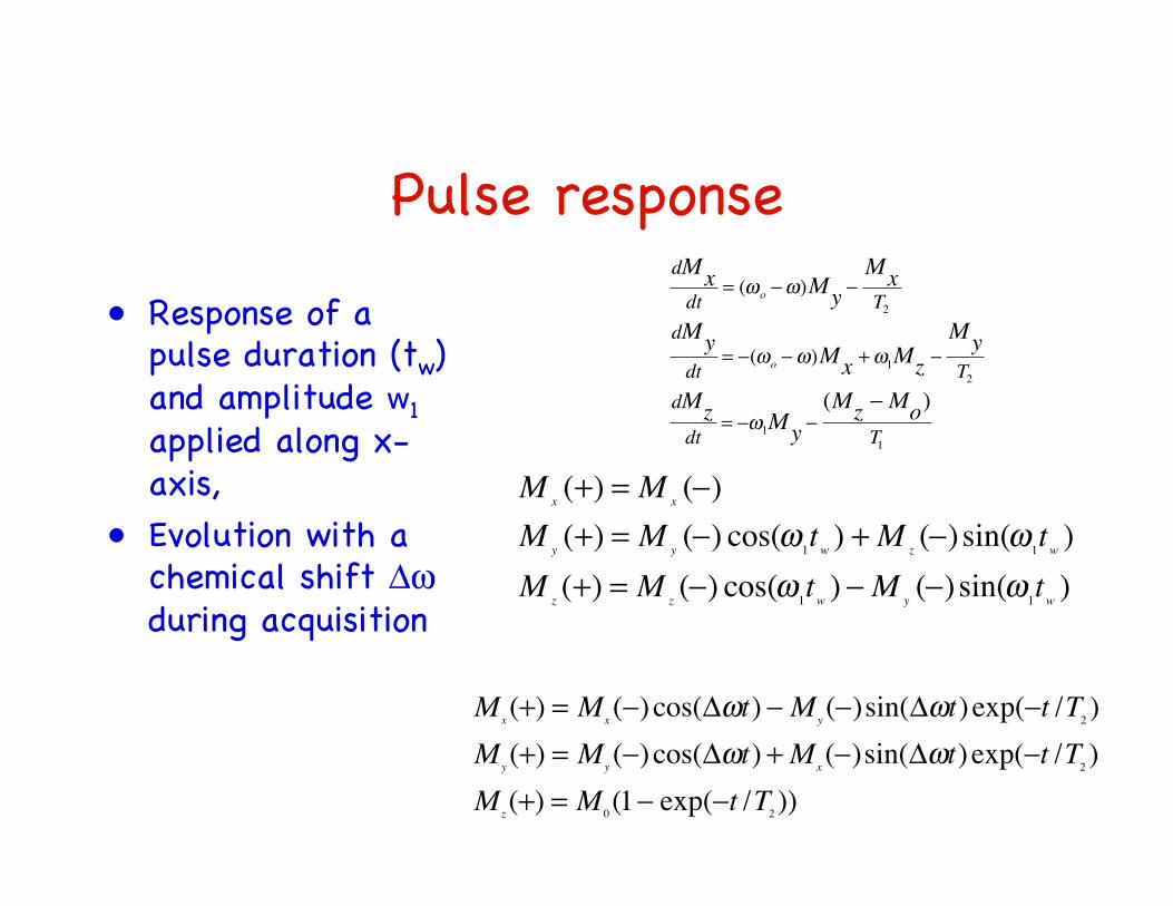
Pulse response�

•  Response of a pulse duration (tw) and amplitude w1 applied along x-axis,�

•  Evolution with a chemical shift Δω during acquisition �

�

M x (+) = M x (−)M y (+) = M y (−) cos(ω1tw ) + M z (−) sin(ω1tw )M z (+) = M z (−) cos(ω1tw ) −M y (−) sin(ω1tw )

�

Mx(+) = M

x(−) cos(Δωt) − M

y(−)sin(Δωt) exp(−t /T

2)

My(+) = M

y(−) cos(Δωt) + M

x(−)sin(Δωt) exp(−t /T

2)

Mz(+) = M

0(1− exp(−t /T

2))

�

dMx

dt= (ω

o−ω)M

y−

Mx

T2

dMy

dt= −(ω

o−ω)M

x+ ω

1Mz−

My

T2

dMz

dt= −ω1My

−

(Mz−M

o)

T1

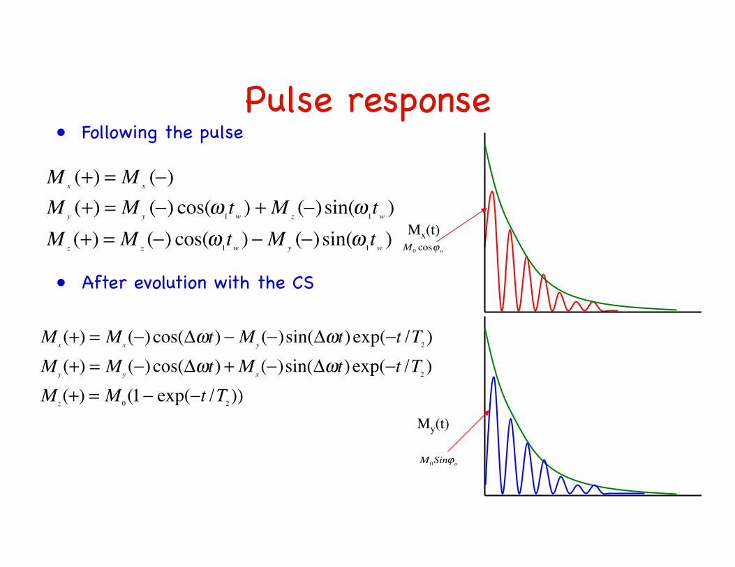
Pulse response�•  Following the pulse�

My(t)

M 0Sinϕo

Mx(t) M 0 cosϕo

�

M x (+) = M x (−)M y (+) = M y (−) cos(ω1tw ) + M z (−) sin(ω1tw )M z (+) = M z (−) cos(ω1tw ) −M y (−) sin(ω1tw )

�

Mx(+) = M

x(−) cos(Δωt) − M

y(−)sin(Δωt) exp(−t /T

2)

My(+) = M

y(−) cos(Δωt) + M

x(−)sin(Δωt) exp(−t /T

2)

Mz(+) = M

0(1− exp(−t /T

2))

•  After evolution with the CS�

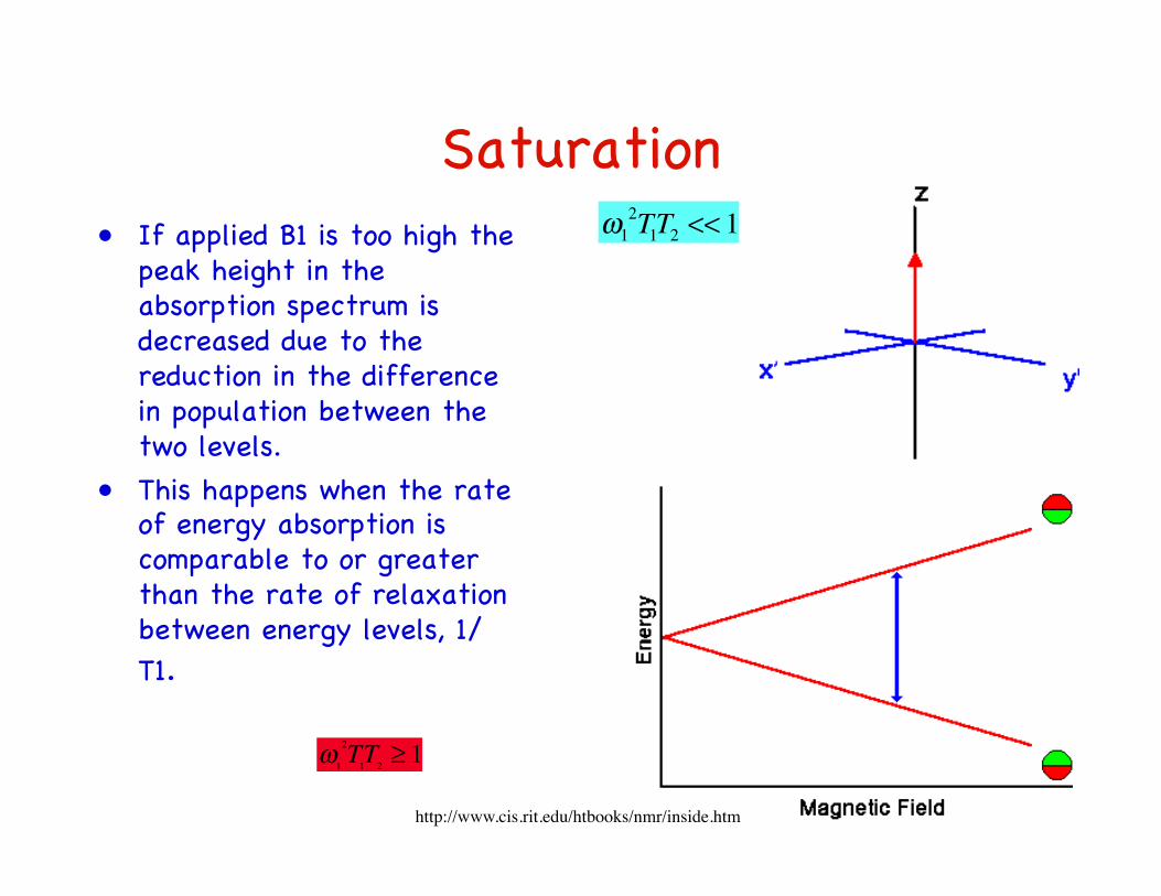
Saturation �•  If applied B1 is too high the

peak height in the absorption spectrum is decreased due to the reduction in the difference in population between the two levels. �

•  This happens when the rate of energy absorption is comparable to or greater than the rate of relaxation between energy levels, 1/T1. �

�

ω1

2T1T2

<< 1

�

ω1

2T1T2 ≥ 1

http://www.cis.rit.edu/htbooks/nmr/inside.htm

Nuclear receptivity�•  In Steady state NMR

experiment the spin system can absorb energy from RF at a rate R is depends on transition probability p, energy level separation, ΔE and population difference Δno �

•  NMR detected signal ~ dMy/dt =R/B1 �

�

R = pΔEΔno ∝ γ 4B0

2NB1

2g(ω) / kT

�

S ∝ R /B1 ∝ γ 4B0

2NB1g(ω) / kT

�

Δno = NΔE /2kTp∝ γ 2B1

2g(ω)ΔE = γBo

�

B1(opt) = (γ 2T1T2 )−1/ 2

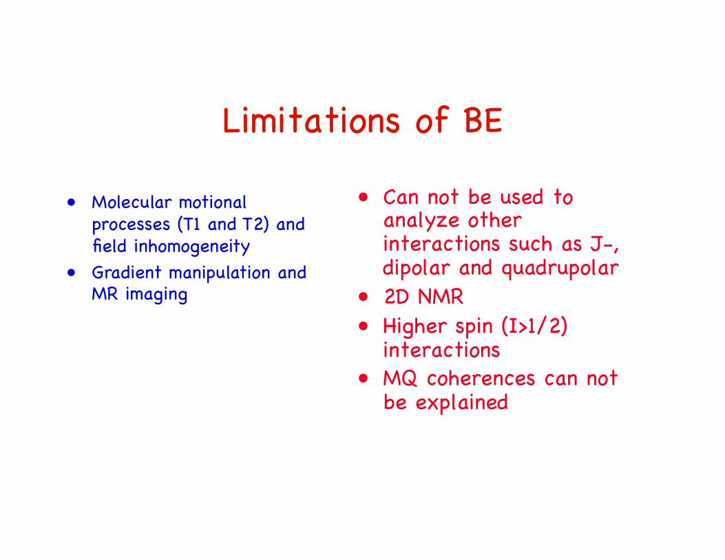
Limitations of BE�

•  Can not be used to analyze other interactions such as J-, dipolar and quadrupolar�

•  2D NMR �•  Higher spin (I>1/2)

interactions�•  MQ coherences can not

be explained�

•  Molecular motional processes (T1 and T2) and field inhomogeneity�

•  Gradient manipulation and MR imaging �