Embed Size (px)
Citation preview

UNIVERSITY OF CALGARY
Storage and Manipulation of Qubits via Controlled Reversible Inhomogeneous
Broadening
by
Michael S. Underwood
A THESIS
SUBMITTED TO THE FACULTY OF GRADUATE STUDIES
IN PARTIAL FULFILLMENT OF THE REQUIREMENTS FOR THE
DEGREE OF MASTER OF SCIENCE
DEPARTMENT OF PHYSICS AND ASTRONOMY
CALGARY, ALBERTA
September, 2008
c© Michael S. Underwood 2008

Abstract
A new variation of the so-called CRIB protocol for quantum memory based on controlled
reversible inhomogeneous broadening is presented. The CRIB protocol is a proposal to
allow quantum states of light to be stored in, and later recalled from, the collective state
of a solid-state atomic ensemble. An introductory discussion explores the theory of the
original protocol, which relies on a hidden time-reversal symmetry in the Maxwell-Bloch
equations. This symmetry is then broken here in a controlled fashion, by considering a
single storage medium as two spatially-distinct segments when recalling the light. The
stored photonic state is recalled from the two segments individually; this results in a
superposition state in which the photon has specified probabilities to have left the storage
medium at one of two times, either ‘early’ or ‘late’. It is shown that the operations of a
beam splitter and phase shifter, the fundamental building blocks of any optical setup, can
be implemented in a quantum memory under this new version of the protocol. Motivation
for the work is drawn from experimental implementations of quantum key distribution,
in particular from the need to perform projective measurements onto certain bases when
making use of the protocol due to Bennett and Brasard in 1984. Simulations of the
systems described herein were performed; their results are presented, and agree with the
theoretical predictions.
ii

Acknowledgements
I would like to thank my parents, Bruce and Joanne, for their continuous and unfailing
support through every stage of my life. They taught me the value of critical thinking,
encouraged an active imagination, and showed me that problems can be looked at as
challenges, and their solutions as rewards unto themselves.
I would also like to thank my wife Katie, whose confidence and support have been
invaluable to me throughout my studies. In particular I could not have finished this
document the same week we got married without the enourmous effort which she put in
to the planning of our wedding, along with my parents-in-law, Debbie and Harold.
Finally I would like to thank my supervisors, Peter and Wolfgang, for their guidance,
dedication, expertise, and advice.
iii

Table of Contents
Abstract ii
Acknowledgements iii
Table of Contents iv
List of Tables vi
List of Figures vii
1 Introduction 11.1 Quantum key distribution . . . . . . . . . . . . . . . . . . . . . . . . . . 1
1.1.1 The BB84 protocol . . . . . . . . . . . . . . . . . . . . . . . . . . 21.1.2 Extending the range of QKD . . . . . . . . . . . . . . . . . . . . 4
1.2 Quantum memory . . . . . . . . . . . . . . . . . . . . . . . . . . . . . . . 61.3 Manipulating qubits . . . . . . . . . . . . . . . . . . . . . . . . . . . . . 71.4 Document structure . . . . . . . . . . . . . . . . . . . . . . . . . . . . . . 9
2 Background 102.1 Theoretical framework . . . . . . . . . . . . . . . . . . . . . . . . . . . . 102.2 The Bloch equations . . . . . . . . . . . . . . . . . . . . . . . . . . . . . 122.3 Maxwell-Bloch equations . . . . . . . . . . . . . . . . . . . . . . . . . . . 15
3 The CRIB protocol 173.1 Finding time-reversal symmetry . . . . . . . . . . . . . . . . . . . . . . . 183.2 Implementation . . . . . . . . . . . . . . . . . . . . . . . . . . . . . . . . 20
3.2.1 Tranverse vs. longitudinal broadening . . . . . . . . . . . . . . . . 223.3 Analysis of CRIB . . . . . . . . . . . . . . . . . . . . . . . . . . . . . . . 23
3.3.1 Forward direction . . . . . . . . . . . . . . . . . . . . . . . . . . . 233.3.2 Backward direction . . . . . . . . . . . . . . . . . . . . . . . . . . 26
3.4 Specific cases . . . . . . . . . . . . . . . . . . . . . . . . . . . . . . . . . 283.4.1 The uniform distribution . . . . . . . . . . . . . . . . . . . . . . . 293.4.2 The Gaussian distribution . . . . . . . . . . . . . . . . . . . . . . 30
3.5 Recall efficiency . . . . . . . . . . . . . . . . . . . . . . . . . . . . . . . . 313.5.1 The magnitude of η . . . . . . . . . . . . . . . . . . . . . . . . . . 323.5.2 Analysis of the recalled pulse . . . . . . . . . . . . . . . . . . . . 333.5.3 Phase of the recalled field . . . . . . . . . . . . . . . . . . . . . . 353.5.4 Output energy . . . . . . . . . . . . . . . . . . . . . . . . . . . . 363.5.5 The ideal case . . . . . . . . . . . . . . . . . . . . . . . . . . . . . 36
iv

0.0 v
4 Breaking time-reversal symmetry 384.1 Splitting the memory . . . . . . . . . . . . . . . . . . . . . . . . . . . . . 39
4.1.1 Optimizing recall efficiency . . . . . . . . . . . . . . . . . . . . . . 414.1.2 The output pulse . . . . . . . . . . . . . . . . . . . . . . . . . . . 424.1.3 Phase difference . . . . . . . . . . . . . . . . . . . . . . . . . . . . 43
4.2 Recall efficiency . . . . . . . . . . . . . . . . . . . . . . . . . . . . . . . . 444.2.1 Dependence on z0 . . . . . . . . . . . . . . . . . . . . . . . . . . . 454.2.2 The ideal case . . . . . . . . . . . . . . . . . . . . . . . . . . . . . 46
4.3 Manipulating qubits . . . . . . . . . . . . . . . . . . . . . . . . . . . . . 494.3.1 Time-bin qubits . . . . . . . . . . . . . . . . . . . . . . . . . . . . 494.3.2 State creation . . . . . . . . . . . . . . . . . . . . . . . . . . . . . 50
5 Simulations 535.1 Forward-propagating Maxwell-Bloch simulation . . . . . . . . . . . . . . 56
5.1.1 Co-moving frame . . . . . . . . . . . . . . . . . . . . . . . . . . . 565.1.2 Runge-Kutta algorithm . . . . . . . . . . . . . . . . . . . . . . . . 585.1.3 Finite difference method . . . . . . . . . . . . . . . . . . . . . . . 595.1.4 Algorithm summary – forward direction . . . . . . . . . . . . . . 605.1.5 Simulating the Bloch vector . . . . . . . . . . . . . . . . . . . . . 61
5.2 Backward-propagating Maxwell-Bloch simulation . . . . . . . . . . . . . 625.2.1 Algorithm summary – backward direction . . . . . . . . . . . . . 63
5.3 Simulating the protocol . . . . . . . . . . . . . . . . . . . . . . . . . . . . 645.3.1 Example simulation – creating two conjugate bases . . . . . . . . 655.3.2 Interfering two time bins . . . . . . . . . . . . . . . . . . . . . . . 675.3.3 Simulating decoherence . . . . . . . . . . . . . . . . . . . . . . . . 695.3.4 Recall in the forward direction . . . . . . . . . . . . . . . . . . . . 70
6 Concluding remarks 73
A Matlab simulation code 74
B Notations and symbols used 81

List of Tables
5.1 Names and values of physical parameters as they appear in the Matlabsimulation code. . . . . . . . . . . . . . . . . . . . . . . . . . . . . . . . . 55
vi

List of Figures
1.1 Original example of BB84 due to Bennett and Brassard in 1984 . . . . . 41.2 Generation of time-bin qubits with an interferometer . . . . . . . . . . . 8
3.1 Construction of a reversible distribution of detunings . . . . . . . . . . . 203.2 The uniform distribution of detunings . . . . . . . . . . . . . . . . . . . 28
4.1 Spacetime diagram of pulse motion . . . . . . . . . . . . . . . . . . . . . 404.2 A demonstrative plot of the output of the double-recall scheme. . . . . . 424.3 Dependence of recall efficiency on z0 . . . . . . . . . . . . . . . . . . . . 474.4 Graphical representation of time-bin states . . . . . . . . . . . . . . . . 50
5.1 Comparison of simulation results arising from different forms of the Maxwell-Bloch equations . . . . . . . . . . . . . . . . . . . . . . . . . . . . . . . 54
5.2 Schematic of the simulation grid . . . . . . . . . . . . . . . . . . . . . . 585.3 Creating an arbitrary output state with a beam splitter and phase shifter 655.4 Creating various states using the double-recall scheme . . . . . . . . . . . 665.5 Interfering the two pulses of a time-bin qubit using the double-recall CRIB
protocol . . . . . . . . . . . . . . . . . . . . . . . . . . . . . . . . . . . . 685.6 Effect of dechoerence on recalled pulse . . . . . . . . . . . . . . . . . . . 695.7 Comparison of double recall results with different decoherence rates . . . 705.8 Simulated recall in the forward direction . . . . . . . . . . . . . . . . . . 715.9 Simulating double-recall in the forward direction . . . . . . . . . . . . . . 72
vii
Chapter 1
Introduction
1.1 Quantum key distribution
In 1984 at a conference in Bangalore, Charles Bennett and Gilles Brassard presented a
protocol which allows the uncertainty principle of quantum mechanics to be exploited
in such a way as to distribute a cryptographic key between two parties [BB84]. What
makes this key distribution protocol unique is that it guarantees no third party can
gain information about the key without advertising their eavesdropping attempt to the
original two. Furthermore, the two communicating parties require only a small amount of
shared secret information in order to prove that they are who they claim to be; besides
this initial authentication they can communicate large volumes of data with absolute
security. Within five years Bennett and Brassard proclaimed “The dawn of a new era
for quantum cryptography: The experimental prototype is working!” [BB89]. By 1991,
Bennett, Brassard, and others had implemented this protocol, now commonly referred
to as ‘BB84’, to distill a secret key between two fictional parties simulated by the same
computer, over a free-space quantum channel 32 cm long [BBB+92]. They also predicted
that existing optical fibres could extend the length of the channel to “at least several
kilometers.”
Also in 1991, Artur Ekert, then working independently, extended the proposal of
Bennett and Brassard by making use of the Einstein-Podolsky-Rosen paradox [EPR35]
to describe an equivalent protocol and prove that its security is inherent in the laws of
quantum mechanics. That is, so long as the quantum theory is not shown to be incomplete
the protocol will remain absolutely secure [Eke91]. The BB84 protocol has become
1
1.1. QUANTUM KEY DISTRIBUTION
widely known in recent years, however it was not generally looked upon as more than an
academic exercise until a Scientific American article published by Bennet, Brassard, and
Ekert not only popularized the idea of ‘quantum cryptography’ but showed the world that
it could be performed in a laboratory environment [BBE92]. Despite being commonly
called quantum cryptography, a more accurate description is given by the term ‘quantum
key distribution’ (QKD), since quantum mechanics plays a role only in distributing a key
between two parties. Once they are in possession of the key, any cryptography performed
with it is classical in nature.
QKD has come a long way since 1984. It is now possible to purchase commercial, off-
the-shelf systems that will provide point-to-point, unconditionally secure channels over
standard telecommunication optical fibres. Such systems include a range of offerings
from id Quantique in Geneva as well as MagiQ Technologies in New York. Of particular
interest to experimental research groups working with any aspect of QKD is the id Quan-
tique Clavis Plug&Play system [id 05], which is designed to be both versatile and stable
while allowing custom control via user-created C++ programs and integration with other
optical components. However, despite all of this progress there is still a basic limitation
to all current QKD implementations. Losses within optical fibres, or even free space,
increase with the distance between two communicating parties. There is a fundamental
limit above which the noise-to-signal ratio, known as the ‘quantum bit error rate’, be-
comes so large that no secret key can be distributed. Furthermore, the rate at which the
key can be generated drops dramatically as this distance limit is approached. Current
implementations such as the Plug&Play system state limits on the order of 100 km.
1.1.1 The BB84 protocol
There are many extant descriptions of the BB84 protocol and its derivatives. Those of a
pedagogical nature include the textbooks by Nielsen and Chuang [NC00] and by Le Bellac
2

1.1. QUANTUM KEY DISTRIBUTION
[LB06]. This is not the place for another in-depth discussion of the protocol, yet some
parts of this work are strongly motivated by aspects of its experimental implementation.
Therefore it will be useful to provide a summary of the key points that allow BB84
to provide unconditional security. For simplicity it will be assumed that detectors and
transmission lines are perfect.
In discussions of cryptographic protocols is is common to give names to the parties
involved, typically assigned alphabetically. Following the common standard, consider a
scenario in which Alice and Bob wish to generate a secret key without meeting, and
with certainty that the notorious eavesdropper Eve gains no information from them. In
order to do so, Alice sends to Bob a photon that is linearly polarized along one of four
axes, aligned at 0 (horizontal), π/2 (vertical), and ±π/4 (±diagonal) with respect to
the horizontal axis. Her choice of axis is random, and when Bob receives the photon he
measures its polarization in either the horizontal-vertical basis or the ±diagonal basis,
also chosen randomly. He then publicly announces to Alice which basis he chose, but
not the result of his measurement. If she chose an axis from the same basis then she
knows with certainty his measurement result, and they share a key bit. If the photon
was originally prepared along one of the other two axes, she tells Bob to discard his
result. This process repeats until Alice and Bob share enough key bits to safely encrypt
their message. In order to determine whether Eve attempted to listen, Alice and Bob
publicly declare the values of a subset of their key bits. If they all match, then Alice and
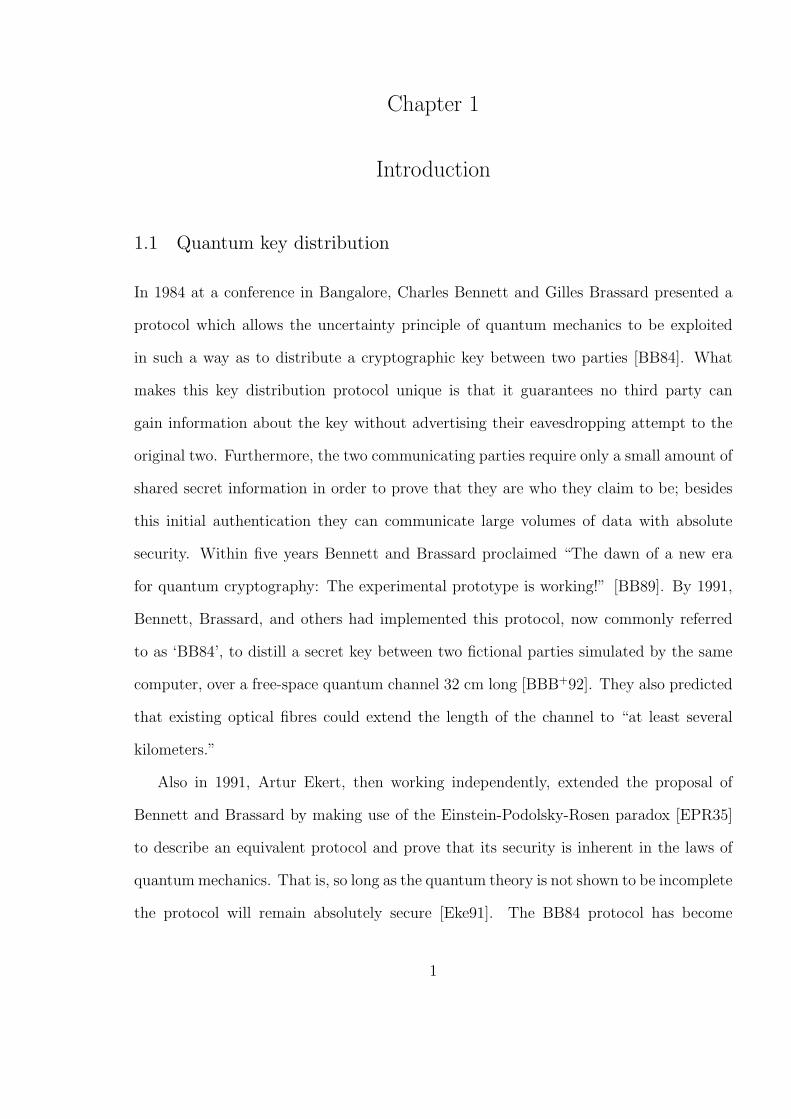
Bob can be confident that their remaining secret bits also match. Figure 1.1 contains a
reproduction of the hypothetical run of the protocol as originally presented in Bangalore
by Bennett and Brassard.
3

1.1. QUANTUM KEY DISTRIBUTION
1.1.2 Extending the range of QKD
As already mentioned, existing QKD implementations have a finite range, due to the
fact that no method of transmission can be truly lossless, and since the losses increase
with distance while the level of detector noise remains constant, the signal-to-noise ratio
approaches zero. This problem is circumvented in classical telecommunications by the
use of repeaters – devices which read a signal before it has degraded to uselessness, then
amplify and re-transmit it. By chaining such repeaters together, there is no limit to the
distance over which classical communications can occur. Unfortunately in the case of
quantum information, the same property that guarantees security also prevents the use
of traditional repeaters; any attempt to read the information in order to amplify it will
instead destroy the quantum nature of the state. However, there are proposals for other
methods to solve this problem. The simplest theoretical solution is to have a trusted site
every 100 km or so along the desired transmission path. Each of these sites can then
create a secret key with its neighbours, and ultimately pass the message the entire length
of the chain. In practice of course, it is dangerous to assume that such a sequence of sites
will exist, and impractical on a large scale to hope that all possible pairs of people who
wish to communicate across a network will trust every node in the network.
Figure 1.1: The original example of the BB84 protocol, reproduced from the paper ofBennett and Brassard [BB84]. The bases are labeled ‘R’ for rectilinear, corresponding tothe axes at 0 and π/2; and ‘D’ for diagonal, those at ±π/4.
4
1.1. QUANTUM KEY DISTRIBUTION
A more promising method that allows arbitrary extension of the distance over which
keys can be generated, without requiring any additional trusted sites, makes use of so-
called quantum repeaters [BDCZ98, DLCZ01]. As with quantum cryptography, the term
‘quantum repeater’ is something of a misnomer; the proposal is however to provide a
method of obtaining the result that a repeater would offer, if the quantum no-cloning
theorem didn’t forbid it [WZ82]. What the protocol actually allows for is also known
as entanglement swapping, which better describes the physical mechanism behind its
achievement. Briefly, the protocol functions as follows. Two parties who wish to com-
municate securely but are too far apart to implement QKD each generate a pair of
maximally-entangled photons, keeping one half of the pair and sending the other half to
a centrally-located third party. When both photons have arrived, a Bell-state measure-
ment is performed on them. This results in the other halves of the original photon pairs
becoming entangled, which in turn allows a QKD protocol to be enacted. Obviously un-
der this description the maximum distance over with QKD can be implemented is merely
doubled, but the process can be easily chained together as many times as necessary to
cover an arbitrary distance. It is worth noting that the two communicators do not need
to trust the third party (or parties, in the case of multiple steps between them) in order
for the protocol to work.
The integral component that allows the entanglement-swapping protocol to work
efficiently over large distances is a method by which a photon can be ‘paused’ at a certain
location. This then allows the two communicators to each store a photon while waiting
for the protocol to complete. There is also the possibility that either of the photons
might not arrive at the central location, due to losses in the transmission medium. The
probability of successfully implementing the protocol increases when it is possible to store
one photon until the other has arrived. As may be evident by now, the role of photons in
quantum information in general, and in QKD specifically, is to be information carriers.
5

1.2. QUANTUM MEMORY
This pausing of the photon is therefore seen as analogous to storing or ‘remembering’ the
photon’s information, so devices capable of performing this task are generally referred to
as ‘quantum memories’.
1.2 Quantum memory
The goal of any quantum memory for photons is to keep in one place, for a specified
period of time, the information encoded in a quantum state of light. After the desired
time has passed, the information should then continue to propagate at the speed of
light. One method for achieving this goal is to radically slow or even stop the light by
affecting the refractive index of a medium. Achieving this is generally based on the idea
of electromagnetically-induced transparency (EIT) [HFI90, BIH91]. The phenomenon of
EIT allows an otherwise-opaque medium to be rendered transparent to a given probe
pulse by use of a strong control field. If the control field is switched off while the probe
is still inside the medium, the pulse cannot continue propagating effectively, and so
remains trapped within the medium until the control is switched back on. This was first
achieved by Hau et al. in 1999 when they slowed light to 17 m/s [HHDB99]. A year
later it was proposed to make use of this method as a quantum memory [FL00], and
experimental storage of classical light fields in trapped Sodium [LDBH01] and in atomic
Rubidium vapour [PFM+01] soon followed. Storage of quantum states of light has also
been achieved more recently by various groups [AEW+05, CMJ+05, AFK+08].
Another common method for attempting to store quantum states of light is to co-
herently transfer, in a reversible manner, the relevant quantum information from the
state of the light to the state of either a single trapped atom or a solid-state ensemble of
many atoms. The case of interactions between a photon and a single trapped atom is the
domain of cavity quantum electrodynamics; Jeff Kimble’s group has proposed and begun
6

1.3. MANIPULATING QUBITS
experimental investigations into such a memory [BBM+07]. When many more atoms
are involved, the system can be treated as a statistical ensemble. It is in this regime
that protocols based on controlled reversible inhomogeneous broadening of the medium’s
absorption profile (CRIB) can be employed, and it is this basis for quantum state storage
which the current work explores and to which it adds. As it is the foundation for the
current work, a detailed description of the CRIB protocol is left until Chapter 3, wherein
a detailed analysis is presented, following the work of Sangouard et al. [SSAG07], while
including calculations in a more general, non-ideal setting.
1.3 Manipulating qubits
Fundamental not only to QKD but to any quantum information processing application
is the ability to manipulate qubits. When the qubits are encoded in photons, this obvi-
ously entails an optical setup of some sort. It has been shown that an arbitrary optical
setup can always be decomposed into a combination of beam splitters and phase shifters
[RZBB94], which can therefore be thought of as fundamental units or building blocks for
manipulating photonic states. For example, in the BB84 protocol it is necessary to be
able to prepare a set of four appropriate states, and perform projection measurements
onto each of them. The most intuitive of these sets of states is generally held to be that
described in Section 1.1.1, based on polarization. This choice is not well adapted for
communications over standard optical fibres though, as fibres may not preserve the state
of polarization of transmitted light. A more common approach is to make use of time
windows, or bins, to define qubits. Instead of associating the bit values 0 and 1 with hor-
izontal and vertical polarization respectively, as done in Figure 1.1, the bits 0 and 1 can
be assigned to photons arriving in the first (early) or second (late) time bin, for example
[BGTZ99]. This then implies that the analogue of the ±π/4 polarization states must be
7
1.3. MANIPULATING QUBITS
¡¡¡ @
@@
¡¡¡ @
@@
-
?
ϕ
Single-photon
input state
Vacuum input state
Variable beam splitters
Phase shifter Superposition
output states
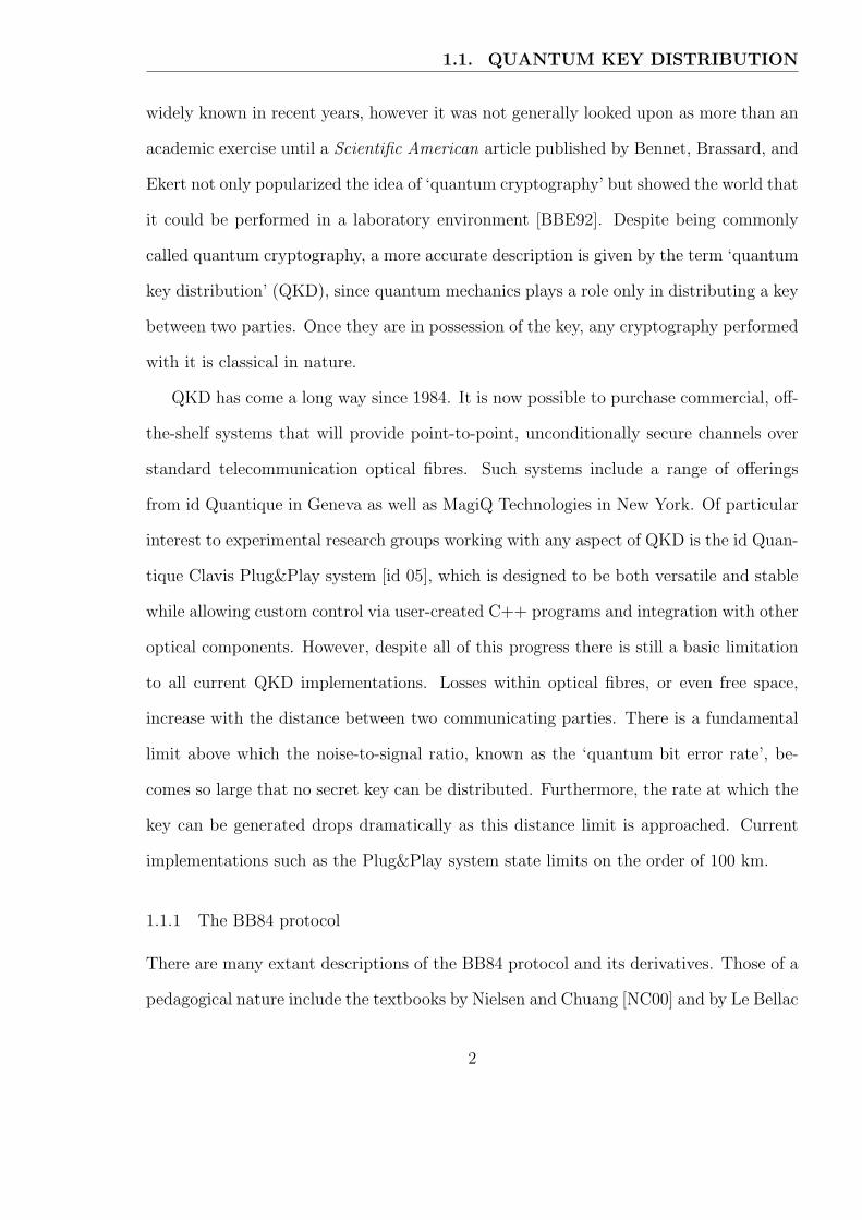
Figure 1.2: A schematic representation of the traditional method of making a measure-ment in a time-bin basis. A photon in an arbitrary superposition of two time bins is sentinto the first beam splitter. If the path-length difference between the two arms corre-sponds to the time delay between the two time bins, there will be three bins to considerat each output.
given by a photon in a superposition of being early and late. In general the creation and
measurement of such a state is achieved by use of an interferometer, as shown in Figure
1.2, which is composed of two beam splitters and a phase shifter. This method works well
for creating the states, and also works perfectly, in theory, for making measurements. It
also works well in practice, however, in order for Alice and Bob to obtain useful results
they must each have an interferometer, and the path-length differences of the pair must
be stabilized to within a small fraction of the photon’s wavelength over distances of up
to 100 km. The need for this stabilization arises due to the fact that Alice and Bob
must use the same definition of |early〉 and |late〉 in order for the protocol to work. This
can already be achieved experimentally, although a method that removed the need for
long-distance stabilization and which made use of a device with other applications in
QKD would have distinct advantages. Another method of manipulating states, known as
Raman adiabatic transfer of optical states (RATOS), has been proposed in the context
of EIT [AML06]. The RATOS scheme makes use of multiple optical control fields and an
ensemble of atoms that possess an energy level structure containing a so-called multi-Λ
configuration in order to transfer photons between two optical modes.
8
1.4. DOCUMENT STRUCTURE
In Chapter 4 a new method for performing the same tasks as beam splitters and phase
shifters is presented. It also makes use of atomic ensembles, although being based on a
modification of the CRIB protocol means that it requires only a two-level system. This
new method allows the same physical device to be employed as a quantum memory, a
beam splitter, and a phase shifter. It requires only the ability to control classical static
electric fields, so has the potential to be experimentally simpler than the interferometer-
based methods currently in use. Furthermore, the method is also able to prepare the
requisite BB84 states.
1.4 Document structure
In Chapter 2 the background theory required for a discussion of the CRIB protocol is
reviewed. This consists primarily of the Maxwell-Bloch equations, and is where many
notations and concepts are introduced. As already mentioned, Chapters 3 and 4 provide
a detailed investigation of the CRIB protocol in a non-ideal medium, and the proposed
modifications to it that allow arbitrary time-bin qubits to be created and the tasks of
a beam splitter and phase shifter to be replicated in the storage device. With the new
protocol well-defined, Chapter 5 presents the method used in this work to simulate the
evolution of the modified system, along with various results from the simulations and
their interpretations. Finally some concluding remarks can be found in Chapter 6. The
code that was used to create the simulation results is presented in Appendix A, and a
summary of symbols and notation can be found in Appendix B.
9

Chapter 2
Background
2.1 Theoretical framework
A description of the CRIB protocol relies on a description of the interaction of a weak
electric field with an ensemble of absorbers. Thus before investigating the protocol in
detail, a theoretical framework able to describe such an interaction must be established.
The appropriate theory is contained in the Maxwell-Bloch equations, which describe the
interaction of a classical light field and an ensemble of quantized two-level atoms. In the
present case the light field is assumed to be a pulse of finite temporal width. This pulse
is likely to come from a laser so it is well justified to consider a one-dimensional electric
field of the form
Ef(z, t) = εEf(z, t)e−i(ωLt−kz) + c.c. , (2.1)
where Ef is a function describing the pulse envelope, and is assumed to be real. Here
the subscript ‘f’ refers to a forward-propagating pulse, i.e. one moving in the positive z
direction; later ‘b’ subscripts will be introduced for a backward-moving pulse.
The state of a single two-level atom can be described by a density operator ρ(t) that
evolves according to the Schrodinger equation. This leads to the definition of the Bloch
vector, r(t) =3∑i=1
ri(t)ei, specified by the three components
r1 = 2Re(ρ12) , (2.2a)
r2 = 2Im(ρ12) , (2.2b)
r3 = ρ22 − ρ11 . (2.2c)
The chosen basis in which to work is that of the atomic Hamiltonian, HA, with |1〉 and |2〉
10

2.1. THEORETICAL FRAMEWORK
representing the ground state and excited state, respectively. For example ρ12 = 〈1|ρ|2〉.Such an atom will have a resonance frequency ω0, from which the laser is detuned by an
amount ∆. That is, for i ∈ 1, 2, HA|i〉 = ~ωi|i〉 and
ω2 − ω1 =: ω0 = ωL + ∆ . (2.3)
The absorption profile of the medium as a whole is equivalent to a distribution of spectral
components within the medium, given by a function g(∆) satisfying
∫ ∞
−∞d∆ g(∆) = 1 ; (2.4)
that is, 100% of the atoms must have some detuning. Each atom has some natural
linewidth centred on its resonance frequency. This width, assumed to be the same for
all the atoms in the medium, is known as the ‘homogeneous linewidth’ and denoted
Γh. However, in any solid medium there are localized stresses and strains which modify
the energy levels of individual atoms, resulting in different resonance frequencies for
different absorbers. In particular this is true in the case of rare-earth-ion-doped crystals
and locally crystalline media, such as optical fibres. The stresses and strains create
a spatially inhomogeneous potential, resulting in variations of the resonant frequencies
present in the ensemble. The net result of this is an absorption profile for the medium
that is wider than the profile of any individual absorber within it; the width of this profile
is the ‘inhomogeneous linewidth’ and is denoted Γih. In addition, external factors such as
electric or magnetic fields may further broaden the range of transition frequencies present
within the sample. This results in a cumulative absorption profile that is significantly
wider than the individual profile of any given absorber. This profile in frequency space,
relative to the laser frequency ωL, is the detuning profile g(∆).
If the medium as a whole is now considered to be comprised of a continuum of two-
level atoms, with a corresponding Bloch vector at each position z and for each detuning
∆, distributed according to g(∆), then the state of the medium can be described by
11
2.2. THE BLOCH EQUATIONS
a continuous field of Bloch vectors, r(z, t, ∆). With this description of the medium its
polarization P(z, t), appearing in Maxwell’s equations, is given by
P(z, t) =N
2
∫ ∞
−∞d∆ g(∆)µ12 [r1(z, t, ∆)− ir2(z, t, ∆)] + c.c. (2.5)
where N is the density of atomic dipoles in the medium, and the atomic dipole moment
µ12 = 〈1|µ|2〉 is the off-diagonal element of the dipole operator µ. This expression
suggests a definition which will prove to be convenient, that of the atomic polarization
σ(z, t, ∆) := r1(z, t, ∆)− ir2(z, t, ∆) . (2.6)
As the light propagates within the medium it induces a wave of polarization whose phase
will match that of the electric field. It is therefore useful to further define slowly-varying
forward- and backward-moving components of the polarization via
σ(z, t, ∆) =: σf(z, t, ∆)e−i(ωLt−kz) + σb(z, t, ∆)e−i(ωLt+kz) . (2.7)
Of course, so long as there has only been a pulse moving in the forward direction σb will
vanish.
2.2 The Bloch equations
The goal of this chapter is to derive a set of equations that govern the evolution of a
light pulse (or more specifically its envelope function) within a solid-state medium, and
of the medium itself. These will be the well-known Maxwell-Bloch equations [MW95].
The first step will be to derive the evolution of the atomic polarization in the presence of
an external electric field. To begin, consider the behaviour of the Bloch vector under the
influence of an interaction Hamiltonian HI . The equations of motion for r are straight-
forward to derive from Schrodinger’s equation; they are the Bloch equations [Blo46], a
12
2.2. THE BLOCH EQUATIONS
set of coupled differential equations,
∂tr1 =2
~Im
(〈1|HI |2〉
)r3 − ω0r2 , (2.8a)
∂tr2 = −2
~Re
(〈1|HI |2〉
)r3 + ω0r1 , (2.8b)
∂tr3 = −2
~Im
(〈1|HI |2〉
)r1 +
2
~Re
(〈1|HI |2〉
)r2 . (2.8c)
The case of interest here involves the interaction between the light field and the atomic
dipoles in the medium, and it is assumed that the light is propagating in the forward
direction. The interaction Hamiltonian, HI , is thus of the well-known form
HI = −µ · Ef . (2.9)
The result of the inner product in (2.9) depends on the nature of the atomic transition and
on the polarization of the light field. It is generally assumed that the atomic transition
of the medium is known and that the polarization state of the light can be chosen to
maximize the probability of the transition occuring. That is, linearly-polarized light
will be chosen for the case of an atomic ∆m = 0 transition, while circularly-polarized
light will be selected given a ∆m = ±1 transition. These two cases result in different
equations of motion for the Bloch vector, but under the rotating wave approximation
they become equivalent [MW95]. This approximation consists of neglecting rapidly-
oscillating components which vanish on average over any appreciable time scale. The
resulting equations are,
∂tr1 = −2℘Ef
~sin(ωLt− kz)r3 − ω0r2 , (2.10a)
∂tr2 =2℘Ef
~cos(ωLt− kz)r3 + ω0r1 , (2.10b)
∂tr3 =2℘Ef
~sin(ωLt− kz)r1 − 2℘Ef
~cos(ωLt− kz)r2 , (2.10c)
where
℘ := µ12 · ε∗ (2.11)
13

2.2. THE BLOCH EQUATIONS
can be assumed to be real based on an appropriate choice of light polarization for the
type of atomic transition.
There is a final simplifying step that can be made, that of switching into the so-called
rotating frame. This is achieved by noting that most of the terms in these equations of
motion oscillate with frequency ωLt− kz, and therefore choosing to define a pair of new
components r′1 and r′2 via
r′1 − ir′2 := (r1 − ir2) ei(ωLt−kz) . (2.12)
Note that this definition is equivalent to those anticipated by (2.6) and (2.7) for the case
in which there is no backward-moving polarization wave, σb = 0, namely
σf = σei(ωLt−kz) . (2.13)
Furthermore, the definition of r′, the Bloch vector in the rotating frame, is completed
by setting r′3 := r3. The equations of motion for the components of this vector are then
given by
∂tr′1 = ∆r′2 , (2.14a)
∂tr′2 = −∆r′1 +
2℘Ef
~r′3 , (2.14b)
∂tr′3 = −2℘Ef
~r′2 . (2.14c)
From (2.12) and (2.13) it is clear that σf = r′1 − ir′2; from this and (2.14) the equation of
motion for σf is found to be
∂tσf(z, t, ∆) = i∆σf(z, t, ∆)− i2℘
~Ef(z, t)r3(z, t, ∆) . (2.15)
In the low-excitation limit, eminently valid for the case of a large number of atoms
interacting with a weak field equivalent to a small number of photons, the vast majority
of the atoms remain unexcited. As can be seen from (2.2c) this means that r3 ≈ −1.
14

2.3. MAXWELL-BLOCH EQUATIONS
Under this assumption the equation of motion for the polarization becomes
∂tσf(z, t, ∆) = i∆σf(z, t, ∆) + i2℘
~Ef(z, t) . (2.16a)
When the only electric field present in the medium is a backward-propagating pulse,
similar considerations result in the same equation of motion for the corresponding polar-
ization wave,
∂tσb(z, t, ∆) = i∆σb(z, t, ∆) + i2℘
~Eb(z, t) . (2.16b)
These two equations describe the behaviour of the ensemble of dipoles in the medium in
the presence of an electric field. The next step will be to determine the behaviour of the
electric field in the presence of this atomic polarization.
2.3 Maxwell-Bloch equations
A good starting point when examining the behaviour of an electromagnetic field is always
provided by Maxwell’s equations. They yield the wave equation for light in a polarized
medium, (∂2z −
n2
c2∂2t
)Ef(z, t) =
1
ε0c2∂2tP(z, t) . (2.17)
Here n denotes the refractive index of a transparent background medium in which the
medium with polarization P is embedded. In particular this may represent a polarizable
ensemble of rare-earth ions doped into a glass or crystal. The polarization can be ex-
pressed in terms of the collective state of the atomic dipoles using (2.5). Along with the
slowly-varying envelope approximations
∣∣∂2t Ef
∣∣ ¿ ωL |∂tEf| ¿ ω2L |Ef| and
∣∣∂2zEf
∣∣ ¿ k |∂zEf| ¿ k2 |Ef| (2.18)
this results in the paraxial wave equation
(n
c∂t + ∂z
)Ef(z, t) = i
ωLN℘
4ε0nc
∫ ∞
−∞d∆ g(∆)σf(z, t, ∆) . (2.19a)
15
2.3. MAXWELL-BLOCH EQUATIONS
Under the same conditions the backward-moving field is governed by
(n
c∂t − ∂z
)Eb(z, t) = i
ωLN℘
4ε0nc
∫ ∞
−∞d∆ g(∆)σb(z, t, ∆) . (2.19b)
At this point there are two possibile paths forward. The first results in the full, general
form of the Maxwell-Bloch equations: from the definition of σf, (2.19a) is equivalent to
(n
c∂t + ∂z
)Ef(z, t) = i
ωLN℘
4ε0nc
∫ ∞
−∞d∆ g(∆) [r′1(z, t, ∆)− ir′2(z, t, ∆)] (2.20)
which, on comparison of real and imaginary parts, simplifies to
(n
c∂t + ∂z
)Ef(z, t) =
ωLN℘
4ε0nc
∫ ∞
−∞d∆ g(∆)r′2(z, t, ∆) . (2.21)
The combination of (2.21) and the evolution of r′2 as governed by (2.14) yields the
Maxwell-Bloch equations (a similar result holds for the backward-moving components).
On the other hand, one can make use of (2.16) to evolve the atomic polarization in
the low-excitation limit, in which case the light field is governed by (2.19). These coupled
differential equations provide a simplified form of the Maxwell-Bloch equations that is
particularly useful for describing the CRIB protocol for quantum memory.
In order to further simplify the notation used it is common to define the Rabi fre-
quency
Ω(z, t) :=2℘
~E(z, t) (2.22)
and to define a constant
β :=ωLN℘2
2ε0~nc. (2.23)
The Maxwell-Bloch equations are presented using these conventions in the next chapter,
along with a detailed description and analysis of the CRIB protocol. While Ω has units
of Hz, it differs from the electric field only by a constant factor. For this reason one may
refer to Ω as the light field, and in fact this is done frequently in the subsequent chapters.
16

Chapter 3
The CRIB protocol
The CRIB protocol for quantum memory describes a method by which a given state of
light can be stored in the coherences of an ensemble of atomic dipoles embedded in an
otherwise-transparent solid. The process is similar to that of photon echoes [KAH64,
AKH66]; light is absorbed coherently by the ensemble, the members of which begin to
dephase with respect to one another. A hidden time-reversal symmetry of the system is
then exploited to cause the atoms to begin rephasing, so that a time-reversed copy of the
input light is re-emitted, propagating in the opposite direction [MK01, NK05, KTG+06,
SSAG07]. Modifications to the original protocol that allow for high-efficiency recall in
the forward direction have also been propsed, and initial experimental tests have yielded
recall efficiencies of up to 15% [ALSM06, HLA+08].
A detailed description of the CRIB protocol is the subject of the following sections,
but it is instructive to begin with an outline of its general form. A light pulse to be
stored travels forward in the positive z direction through a transparent medium toward
the storage medium, which contains an ensemble of atomic dipoles. These absorbers exist
for z ∈ [0, L], where L is the length of the medium. Inside the medium some portion of
the pulse gets absorbed; ideally absorption is complete, but for finite optical depth some
percentage of the pulse will exit the medium at z = L and be lost from the system. Some
time after the absorption it is possible to perform some action that results in the recall
of the pulse, which exits the medium at z = 0 propagating backward, in the negative z
direction.
17
3.1. FINDING TIME-REVERSAL SYMMETRY
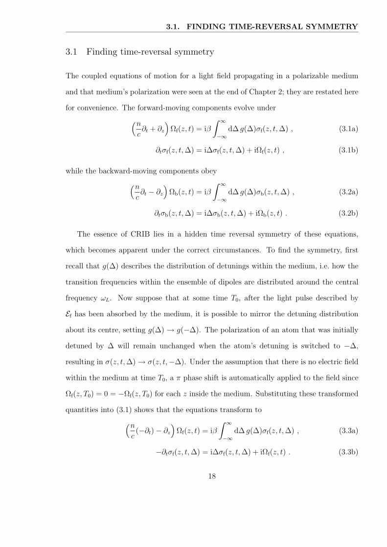
3.1 Finding time-reversal symmetry
The coupled equations of motion for a light field propagating in a polarizable medium
and that medium’s polarization were seen at the end of Chapter 2; they are restated here
for convenience. The forward-moving components evolve under
(n
c∂t + ∂z
)Ωf(z, t) = iβ
∫ ∞
−∞d∆ g(∆)σf(z, t, ∆) , (3.1a)
∂tσf(z, t, ∆) = i∆σf(z, t, ∆) + iΩf(z, t) , (3.1b)
while the backward-moving components obey
(n
c∂t − ∂z
)Ωb(z, t) = iβ
∫ ∞
−∞d∆ g(∆)σb(z, t, ∆) , (3.2a)
∂tσb(z, t, ∆) = i∆σb(z, t, ∆) + iΩb(z, t) . (3.2b)
The essence of CRIB lies in a hidden time reversal symmetry of these equations,
which becomes apparent under the correct circumstances. To find the symmetry, first
recall that g(∆) describes the distribution of detunings within the medium, i.e. how the
transition frequencies within the ensemble of dipoles are distributed around the central
frequency ωL. Now suppose that at some time T0, after the light pulse described by
Ef has been absorbed by the medium, it is possible to mirror the detuning distribution
about its centre, setting g(∆) → g(−∆). The polarization of an atom that was initially
detuned by ∆ will remain unchanged when the atom’s detuning is switched to −∆,
resulting in σ(z, t, ∆) → σ(z, t,−∆). Under the assumption that there is no electric field
within the medium at time T0, a π phase shift is automatically applied to the field since
Ωf(z, T0) = 0 = −Ωf(z, T0) for each z inside the medium. Substituting these transformed
quantities into (3.1) shows that the equations transform to
(n
c(−∂t)− ∂z
)Ωf(z, t) = iβ
∫ ∞
−∞d∆ g(∆)σf(z, t, ∆) , (3.3a)
−∂tσf(z, t, ∆) = i∆σf(z, t, ∆) + iΩf(z, t) . (3.3b)
18

3.1. FINDING TIME-REVERSAL SYMMETRY
It is now clear that under time reversal, t → −t, these equations become
(n
c∂t − ∂z
)Ωf(z,−t) = iβ
∫ ∞
−∞d∆ g(∆)σf(z,−t, ∆) , (3.4a)
∂tσf(z,−t, ∆) = i∆σf(z,−t, ∆) + iΩf(z,−t) . (3.4b)
On comparison with (3.2) it can be seen by making the identifications
Ωb(z, t) = Ωf(z,−t) and σb(z, t, ∆) = σf(z,−t, ∆) (3.5)
that the equations of motion for a forward-moving pulse have been transformed into
those for a time-reversed copy of the same pulse propagating in the backward direction.
That is, light that has been absorbed while propagating in the forward direction can be
recalled from the medium after some delay; the field will be re-emitted propagating in
the backward direction. This means that the system can be used as a memory for storing
the light if a method can be found for causing the equations of motion for the system to
switch from (3.1) to (3.2). There are indeed methods for doing just that, and they will
be investigated in the next sections.
Before proceeding though one further requirement for triggering the recall of the pulse
must be noted; there is a subtlety in making the assignment σb(z, t, ∆) = σf(z,−t, ∆).
Recall the definition (2.7) of the components of the atomic polarization in the medium:
σ(z, t, ∆) = σf(z, t, ∆)e−i(ωLt−kz) + σb(z, t, ∆)e−i(ωLt+kz) . (3.6)
It is clear that σf is the component propagating in the +z direction, so in order for the
system to evolve backward a 2kz phase shift must be applied to the medium such that
σb(z, t, ∆)e−i(ωLt+kz) = e−2ikzσf(z,−t, ∆)e−i(ωLt−kz) = σf(z,−t, ∆)e−i(ωLt+kz) . (3.7)
Without this phase shift the polarization wave within the medium, and therefore the
recalled pulse, will continue to propagate in the forward direction, and the time-reversal
symmetry will be lost.
19

3.2. IMPLEMENTATION
Frequency
P(a
bso
rb)
- ¾Γih
(a) Naturally broadened profileof inhomogeneous linewidth Γih
Frequency
P(a
bso
rb)
- ¾Γh
(b) Anti-hole burning results inthe homogeneous linewidth Γh
Frequency
P(a
bso
rb)
¾ -γ
(c) Artificially, reversibly broad-ened profile of width γ
Figure 3.1: Probability for light to be absorbed in the medium as a function of frequencyduring the preparatory stages of the CRIB protocol. (a) Initially each dipole in the stor-age medium has a narrow homogeneous linewidth. The probability for the medium toabsorb a photon at a given frequency depends on the number of dipoles at that frequency(solid lines); collectively this range of resonance frequencies provides a much wider in-homogeneous absorption spectrum (dashed line). For clarity an arbitrary homogeneousline has been picked out (bold line). (b) After employing spectral hole burning tech-niques only a single absorption peak remains, within a certain frequency window. (c)An external electric field gradient is applied to the medium, causing a broadening of theabsorption peak. The total area under the absorption line remains constant as it widens.
3.2 Implementation
The results of the previous section show that a memory based on complete time-reversal
of the input light field can be achieved in a system for which the absorption spectrum can
be controllably reversed, g(∆) → g(−∆). Of course, the linewidth must also be broad
enough to absorb all Fourier components of the incoming pulse. This can obviously not
be achieved with every possible choice for the polarizable medium. In fact there currently
is no definitive choice as to which material provides the best possibility for CRIB. Even
as investigations continue it is unlikely that a single medium will become ubiquitous,
since the choice will still depend on parameters such as the frequency of light to be
stored and the required storage duration. There is agreement that locally crystalline
structures doped with a low concentration of rare-earth ions provide all of the necessary
properties, yet determining what rare-earth element should be added to which medium
is still an active area of research. One potential candidate is Erbium-doped optical fibres
[HSSA+06, Sta08], which are already used extensively in classical telecommunication.
20

3.2. IMPLEMENTATION
Two well-studied rare-earth elements are Europium and Praseodymium, generally doped
into crystals such as Y2SiO5 [Ale07]. The properties of Thulium as the dopant are also
being investigated, in YAG and Y2O3 [Cha08], as well as Erbium-doped Y2SiO5, Y2O3,
LiNbO3, YAG, YAlO3, CaWO4, and SrWO4 [STC+02], and Er3+:LiNbO3 along with
Neodymium-doped YVO4 and Y2SiO5[Sta08].
Because of this wide range of choices, all of which are in the relatively early stages of
investigation, there do not exist ‘typical’ values for many of the parameters involved. For
example, optical coherence times can range from nanoseconds to milliseconds for different
ions. For the purposes of the current discussion, when numerical values are required they
will be taken from the investigation of Erbium as a dopant, performed by Staudt [Sta08].
With that in mind, each ion in the ensemble can have a relatively narrow homogeneous
linewidth as depicted in Figure 3.1, on the order of 50 Hz to a few kHz. However, stresses
and strains within the local crystalline structure have the effect of shifting the central
frequencies of these lines. This results in the medium containing a spectrum of classes of
narrow absorption lines which combine to create a much broader line width (∼1 GHz).
This can be seen graphically in Figure 3.1(a).
The overall natural spectrum of the medium is wide, as required, however it cannot
be reversed about its central frequency. Therefore further preparation of the medium
is needed. A single narrow peak can be obtained via spectral hole burning [Mel05]. In
general this technique uses a high-intensity laser of frequency ωL to optically pump any
ions that have a transition resonant with ωL to an auxiliary long-lived ground state. This
results in the medium becoming temporarily transparent to light of frequency ωL. By
scanning the laser frequency over a range of values, broader transparency windows can
be created. In order to prepare the medium for the CRIB protocol, a narrow peak is left
in the middle of the wider transparency window, as depicted in Figure 3.1(b). Finally,
this line is broadened via an externally applied electric field, ES, that results in a Stark
21

3.2. IMPLEMENTATION
shift of each ion. Due to either the random nature of local stresses and strains within
an amorphous medium, or a gradient in the applied field for the case of crystals, the
absorption frequency resulting from the Stark shift will not be the same for each ion.
The net effect is an inhomogeneously broadened spectrum as shown in Figure 3.1(c).
With this setup the CRIB protocol can now be implemented. When the absorption
profile is artificially broadened, the photon to be stored is sent into the medium. It will be
absorbed and the atoms will begin to dephase with respect to each other. Reversing the
polarity of the externally applied field, ES → −ES, will cause the Stark shift affecting each
ion to also be negated. That is, ions initially detuned by an amount ∆ will be detuned
by −∆ after reversing the field; the collective effect of this over all ions is to transform
g(∆) → g(−∆). A frequently-proposed method for applying the 2kz phase shift to the
ensemble is to apply two counter-propagating π pulses to the medium, transferring the
excited atomic population to an auxiliary long-lived ground state and back. Once the
detunings have been reversed and the phase shift applied, the atoms will begin rephasing,
resulting in the photon re-emerging from the medium.
3.2.1 Tranverse vs. longitudinal broadening
The absorption profiles referred to here, particularly those in Figure 3.1, describe how the
memory medium as a whole absorbs light. There are two distinct ways in which one can
obtain such profiles over a finite length. One method is to create a single absorption peak
at each position z between 0 and L, so that the entire width of the profile g(∆) is only
seen when considering the full length of the medium. This results in a position-dependent
distribution such as
g(∆, z) = δ
[∆− γ
(z
L− 1
2
)], (3.8)
which states that the resonance frequency in the medium varies linearly from −γ/2 at
z = 0 to γ/2 at z = L. Such a distribution is often called ‘longitudinal broadening’ since
22
3.3. ANALYSIS OF CRIB
the profile is only broad when integrated along the propagation direction. This method
has been explored both theoretically and experimentally by the research group of Matt
Sellars in Australia [HLA+08].
The other option occurs if at each position within the medium, which has finite width,
there exist multiple absorbers such that the entire profile g(∆) is present at each z. Such
a position-independent distribution is termed ‘transverse broadening’ due to the fact that
the variation in the profile occurs transverse to the direction of propagation. It was this
type of distribution which was assumed in the initial proposal for a CRIB-based memory
[MK01], and is the subject of the current work. While currently being attempted in at
least two research laboratories, the CRIB protocol based on transverse broadening has
yet to be implemented experimentally.
3.3 Analysis of CRIB
Some initial assumptions about the pulse that we wish to store, Ωf(0, t), must be made.
Clearly the pulse must be assumed to have a finite duration if one expects to store it in
its entirety. In order for decoherence effects to be minimized it is further assumed that
the temporal full-width-at-half-maximum duration of the pulse, δt, is short compared
to T2, the inverse of the optical linewidth. These assumptions imply that the pulse is
localized in time, and it is useful to define tp as the temporal centre of the pulse.
3.3.1 Forward direction
The equations (3.1) and (3.2) that exhibit perfect time reversal symmetry represent the
ideal case of unitary evolution within the system. In reality decoherence effects including
spontaneous emission break unitarity. This can be included in the model of the system
23
3.3. ANALYSIS OF CRIB
via inclusion of the decoherence rate,
Γ2 =1
πT2
. (3.9)
In this case the evolution of the atomic polarization can be stated as
∂tσi(z, t, ∆) = (i∆− Γ2) σi(z, t, ∆) + iΩi(z, t) , (3.10)
for i ∈ f, b. The goal here will be to assume that an input pulse at the start of the
medium has a known temporal shape, Ωf(0, t), and to determine the behaviour of the
light plus atoms as the protocol is performed.
In the work of Sangouard et al. [SSAG07], a similar analysis was performed, but with
the assumption of infinite coherence times, Γ2 = 0. The methods employed in these
sections are motivated by their work, with the added inclusion of a non-zero decay rate.
The first step is to formally integrate the evolution equation (3.10) to find a solution
for σf under the assumption that all atoms are initially in the ground state so that
σf(z,−∞, ∆) = 0. This solution,
σf(z, t, ∆) = i
∫ t
−∞ds e(i∆−Γ2)(t−s)Ωf(z, s) , (3.11)
turns the paraxial wave equation into
(n
c∂t + ∂z
)Ωf = −β
∫ ∞
−∞d∆ g(∆)
∫ t
−∞ds e(i∆−Γ2)(t−s)Ωf(z, s) . (3.12)
Taking the Fourier transform of this partial differential equation (PDE) will turn it into
an ordinary differential equation (ODE) that will be easier to solve. The transformation
results in
(inω
c+ ∂z
)Ωf(z, ω) =
−β√2π
∫ ∞
−∞d∆ g(∆)
∫ ∞
−∞dt e−iωt
∫ t
−∞ds e(i∆−Γ2)(t−s)Ωf(z, s) .
(3.13)
Next, the order of integration over the s-t plane is reversed, and the variable u = t− s is
introduced. This isolates the Fourier transform of the input field and yields an integral
24

3.3. ANALYSIS OF CRIB
which can be evaluated:
(inω
c+ ∂z
)Ωf(z, ω) =
−β√2π
∫ ∞
−∞d∆ g(∆)
∫ ∞
−∞ds Ωf(z, s)
∫ ∞
s
dt e−iωte(i∆−Γ2)(t−s)
(3.14a)
=−β√2π
∫ ∞
−∞d∆ g(∆)
∫ ∞
−∞ds Ωf(z, s)
∫ ∞
0
du e−iω(u+s)e(i∆−Γ2)u
(3.14b)
= −β
∫ ∞
−∞d∆ g(∆)Ωf(z, ω)
∫ ∞
0
du ei(∆−ω)ue−Γ2u . (3.14c)
Due to the assumption that Γ2 is positive, the integral over u converges. This leaves an
ODE with respect to z,
(inω
c+ ∂z
)Ωf(z, ω) = −β
∫ ∞
−∞d∆
g(∆)
Γ2 − i(∆− ω)Ωf(z, ω) . (3.15)
A function of ω is defined to be this integral over ∆ in order to simplify the notation of
the previous expression,
H(ω) :=
∫ ∞
−∞d∆
g(∆)
Γ2 − i(∆− ω), (3.16)
so that the evolution of the Fourier components of the incoming light field can be seen
to evolve according to
∂zΩf(z, ω) = −(inω
c+ βH(ω)
)Ωf(z, ω) . (3.17)
This homogeneous DE is easily solved by
Ωf(z, ω) = e−inωz/ce−βH(ω)zΩf(0, ω) , (3.18)
from which an absorption coefficient can be determined. The intensity of each frequency
component decreases exponentially with distance into the medium,
|Ωf(z, ω)|2|Ωf(0, ω)|2 = e−2βRe[H(ω)]z . (3.19)
25

3.3. ANALYSIS OF CRIB
This leads to the definition of the absorption coefficient
α(ω) := 2βRe [H(ω)] . (3.20)
Note that g(∆), β, and Γ2 are all positive by definition. Thus α is also positive, as it
must be to describe an absorbing medium, since
Re [H(ω)] =
∫ ∞
−∞d∆
g(∆)Γ2
Γ22 + (∆− ω)2
> 0 . (3.21)
3.3.2 Backward direction
Since the medium absorbing the pulse is of finite length L, a time T0 can be chosen at
which no non-negligible portiton of the pulse remains within the medium. There is of
course no backward-moving field at this time either, so it can be safely assumed that
Ωf(z, T0) = Ωb(z, T0) = 0. This time is taken to be the moment at which the detunings
are reversed, g(∆) → g(−∆), and a 2kz phase shift is applied so that σf → σb. The state
of the polarization at t = T0 is given by
σb(z, T0, ∆) = σf(z, T0,−∆) = i
∫ T0
−∞ds e−(i∆+Γ2)(T0−s)Ωf(z, s) =: σ0(z, ∆) . (3.22)
After the detunings have been reversed, the equations of motion for the backward-moving
field are given by
(n
c∂t − ∂z
)Ωb(z, t) = iβ
∫ ∞
−∞d∆ g(∆)σb(z, t, ∆) ,
∂tσb(z, t, ∆) = (i∆− Γ2)σb(z, t, ∆) + iΩb(z, t) .
The polarization is again solved for formally,
σb(z, t, ∆) = σ0(z, ∆)e(i∆−Γ2)(t−T0) + i
∫ t
T0
ds e(i∆−Γ2)(t−s)Ωb(z, s) . (3.23)
Putting this into the paraxial wave equation for the light field results in
(n
c∂t − ∂z
)Ωb(z, t) = iβ
∫ ∞
−∞d∆ g(∆)σ0e
(i∆−Γ2)(t−T0)
− β
∫ ∞
−∞d∆ g(∆)
∫ t
T0
ds e(i∆−Γ2)(t−s)Ωb(z, s) . (3.24)
26

3.3. ANALYSIS OF CRIB
As in the previous section the next step will be to Fourier transform this equation. The
left-hand side and second term on the right-hand side are very similar to (3.12), and the
applicable methods are likewise similar. The additional term in this equation provided
by the non-zero initial condition for σ0 is worth investigating more closely. In order to
relate it to the input pulse, the definition (3.22) is used along with the Fourier transform,
resulting in
iβ√2π
∫ ∞
−∞d∆ g(∆)e−(i∆−Γ2)T0
∫ ∞
−∞dt e−iωte(i∆−Γ2)tσ0
=−β√2π
∫ ∞
−∞d∆ g(∆)e−2i∆T0
∫ ∞
−∞dt
∫ ∞
−∞ds e−iωtei∆(t+s)eΓ2(s−t)Ωf(z, s) . (3.25)
This time a useful substitution is provided by u = t + s, which turns (3.25) into
−β√2π
∫ ∞
−∞d∆ g(∆)e−2i∆T0
∫ ∞
−∞du
∫ ∞
−∞ds e−iω(u−s)ei∆ueΓ2(2s−u)Ωf(z, s) (3.26a)
=−β√2π
∫ ∞
−∞d∆ g(∆)e−2i∆T0
∫ ∞
−∞du e−iωuei∆ue−Γ2u
∫ ∞
−∞ds e−i(−ω+2iΓ2)sΩf(z, s)
(3.26b)
= −βΩf(z,−ω + 2iΓ2)
∫ ∞
−∞du e−(iω+Γ2)u
∫ ∞
−∞d∆ g(∆)ei∆(u−2T0) . (3.26c)
In order to simplify notation again the terms independent of z are grouped into the
definition of a new function,
F (ω) :=
∫ ∞
−∞du e−(iω+Γ2)u
∫ ∞
−∞d∆ g(∆)ei∆(u−2T0) , (3.27)
and the solution (3.18) for Ωf can then be used to continue from (3.26c) with
−βF (ω)Ωf(z,−ω + 2iΓ2) = −βF (ω)e−in(−ω+2iΓ2)z/ce−βH(−ω+2iΓ2)zΩf(0,−ω + 2iΓ2) .
(3.28)
Combined with the Fourier transform of the rest of (3.24), this result yields the following
equation of motion:
∂zΩb(z, ω) =(inω
c+ βH(ω)
)Ωb(z, ω)
+ βF (ω)eiωnz/ce2Γ2nz/ce−βH(−ω+2iΓ2)zΩf(0,−ω + 2iΓ2) .
27
3.4. SPECIFIC CASES
-¾
6
+∆−∆
g(∆)
γ/2−γ/2
HHj
1
γ
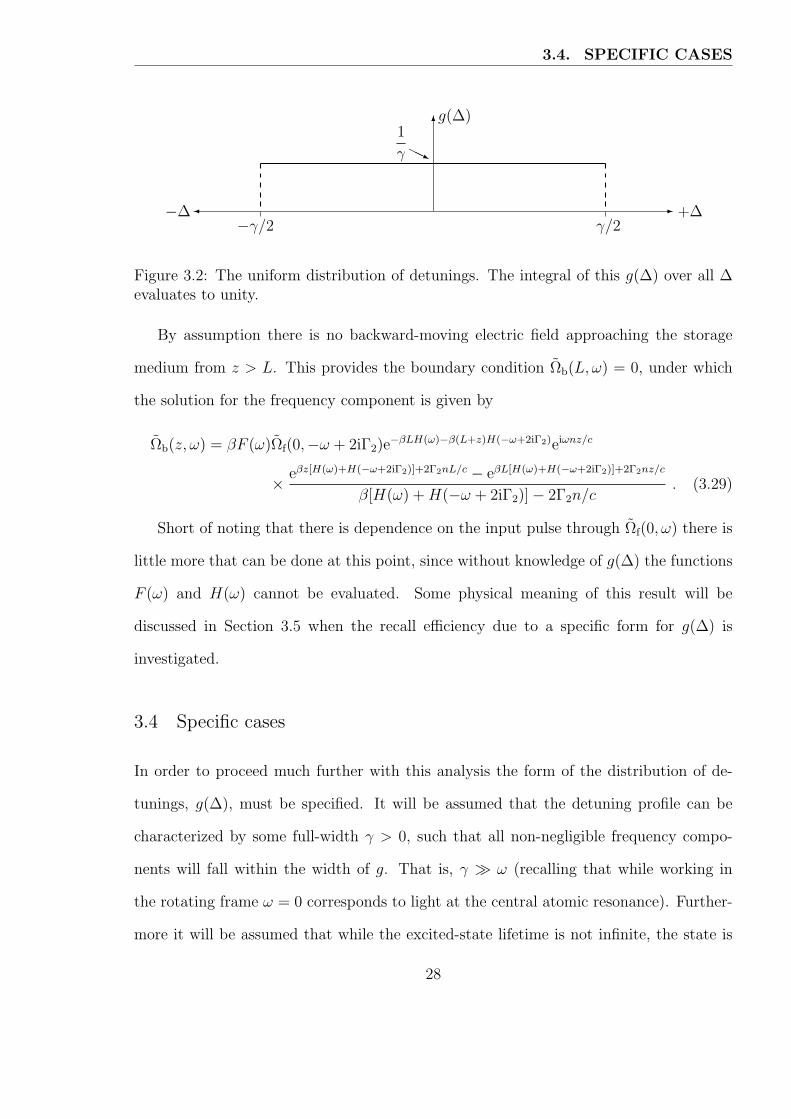
Figure 3.2: The uniform distribution of detunings. The integral of this g(∆) over all ∆evaluates to unity.
By assumption there is no backward-moving electric field approaching the storage
medium from z > L. This provides the boundary condition Ωb(L, ω) = 0, under which
the solution for the frequency component is given by
Ωb(z, ω) = βF (ω)Ωf(0,−ω + 2iΓ2)e−βLH(ω)−β(L+z)H(−ω+2iΓ2)eiωnz/c
× eβz[H(ω)+H(−ω+2iΓ2)]+2Γ2nL/c − eβL[H(ω)+H(−ω+2iΓ2)]+2Γ2nz/c
β[H(ω) + H(−ω + 2iΓ2)]− 2Γ2n/c. (3.29)
Short of noting that there is dependence on the input pulse through Ωf(0, ω) there is
little more that can be done at this point, since without knowledge of g(∆) the functions
F (ω) and H(ω) cannot be evaluated. Some physical meaning of this result will be
discussed in Section 3.5 when the recall efficiency due to a specific form for g(∆) is
investigated.
3.4 Specific cases
In order to proceed much further with this analysis the form of the distribution of de-
tunings, g(∆), must be specified. It will be assumed that the detuning profile can be
characterized by some full-width γ > 0, such that all non-negligible frequency compo-
nents will fall within the width of g. That is, γ À ω (recalling that while working in
the rotating frame ω = 0 corresponds to light at the central atomic resonance). Further-
more it will be assumed that while the excited-state lifetime is not infinite, the state is
28

3.4. SPECIFIC CASES
long-lived so that γ À Γ2.
A physically realistic description of the distribution g(∆) is perhaps provided by a
Gaussian or Lorentzian function. A function that is simple to deal with mathematically
in many of the integrals involved is the uniform distribution which takes on a constant
positive value within a given range and vanishes everywhere else. It can be shown that
under approximations due to the stated assumptions, these three distributions yield
values of H(ω) that differ only by constant factors. For a given width γ and physical
system characterized by β, the uniform distribution attenuates the input pulse more
quickly than the Lorentzian, which in turn absorbs more strongly than the Gaussian
distribution, but otherwise their behaviours are the same. In fact, for any sufficiently
wide and smooth distribution g, the value of g(∆) can be approximated by g(0) for those
∆ that contribute significantly to the behaviour of the system. Therefore any distribution
that satisfies this set of assumptions will result in an absorption coefficient independent
of ω, and differing from α only by a constant factor. For this reason it is sufficient to
consider only the uniform distribution from now on, as is common practice.
3.4.1 The uniform distribution
The previously described uniform distribution, shown in Figure 3.2, can be described
mathematically as
g(∆) =1
γΘ
(γ
2+ ∆
)Θ
(γ
2−∆
). (3.30)
This states that the frequencies of the atoms are uniformly distributed within a window
of width γ centred on ω0 (i.e. on ∆ = 0), and that no atoms exist with detunings outside
that range.
In this case H(ω) as defined in (3.16) evaluates to
H(ω) =2
γarctan
(γ
2
1
Γ2 + iω
). (3.31)
29

3.4. SPECIFIC CASES
Under the given assumptions, γ À |Γ2 + iω| and the argument of arctan is sufficiently
large to approximate
H(ω) ≈ π
γ=⇒ α =
2βπ
γ. (3.32)
The Fourier components of the light field then decay according to (3.18),
Ωf(z, ω) = e−βπz/γe−iωnz/cΩf(0, ω) , (3.33)
which shows that as the field propagates into the medium it evolves as
Ωf(z, t) = e−αz/2Ωf(0, t− nz/c) . (3.34)
This is easily interpreted as follows: The pulse moves through the medium in the positive
z direction with speed c/n; as it does so it retains its original shape, while its amplitude
decays exponentially.
3.4.2 The Gaussian distribution
As already mentioned there is little need to investigate other distributions so long as the
assumptions about their general form are satisfied. It is however informative to show
explicitly that this is true for at least one other case, so in this brief subsection a moment
will be taken to see the effect of choosing to work with the Gaussian distribution,
gG(∆) =e−∆2/2γ2
γ√
2π. (3.35)
The resulting form of H(ω) is again able to be solved exactly,
HG(ω) =1
γ
√π
2e(Γ2+iω)2/2γ2
erfc
(Γ2 + iω
γ√
2
)≈ 1
γ
√π
2, (3.36)
where the final approximation again makes use of the fact that γ À |Γ2 + iω|. The
absorption coefficient is then found from (3.20) to be
αG =2β
γ
√π
2=
α√2π
. (3.37)
30
3.5. RECALL EFFICIENCY
The reason for this can be easily seen from the assumption that the pulse is much narrower
in frequency space than the distribution of detunings. In this case most interaction occurs
roughly at the centre of the distribution; and it is clear to see that
gG(0) =g(0)√
2π. (3.38)
The absorption coefficients reflect this accordingly.
3.5 Recall efficiency
Of particular interest in any memory, quantum or otherwise, is the ability to recall what
has been stored. In this case what is being stored is the input light pulse, Ωf(0, t), and
the field recalled from the medium is likewise Ωb(0, t). From (3.29) it can be seen that
Ωb(0, ω) =βF (ω)e−βL[H(ω)+H(−ω+2iΓ2)]
(e2Γ2nL/c − eβL[H(ω)+H(−ω+2iΓ2)]
)
β[H(ω) + H(−ω + 2iΓ2)]− 2Γ2n/cΩf(0,−ω + 2iΓ2) .
(3.39)
This is still not particularly enlightening, and it is again useful to turn to the uniform
distribution for further analysis. As already seen, in the case of large γ the function H
can be approximated by H(ω) ≈ π/γ. Similarly it can be shown that in the same regime
F (ω) can be approximated by
F (ω) ≈ 2π
γe−2iωT0e−2Γ2T0 . (3.40)
With these approximations the expression for the Fourier components reduces to
Ωb(0, ω) =1− e2Γ2nL/c−2βπL/γ
1− Γ2γn/cβπe−2(iω+Γ2)T0Ωf(0,−ω + 2iΓ2) . (3.41)
The inverse Fourier transform of this expression will finally yield an expression for the
output pulse recalled from the medium. After defining the constant
η := Γ2γn
πβc, (3.42)
31

3.5. RECALL EFFICIENCY
and recalling that the absorption coefficient for the medium is given by α = 2βπ/γ, the
output pulse given by the inverse Fourier transform of (3.41) can be written as
Ωb(0, t) = −e−2Γ2(t−T0) 1− e−αL(1−η)
1− ηΩf(0,−t + 2T0) . (3.43)
Note that in the case of atoms with infinite excited-state lifetimes, Γ2 = 0 ( =⇒ η = 0),
and with the recall being initiated at T0 = 0, this simplifies to
Ωb(0, t) = − (1− e−αL
)Ωf(0,−t) . (3.44)
The simplified result (3.44) is in agreement with the previous work of Sangouard et al.
describing the ideal case [SSAG07]. The new extension to their work resulting from the
less-ideal case described by (3.43) is analyzed here in further detail.
3.5.1 The magnitude of η
While Γ2 has been kept finite throughout this analysis, it has been assumed that the
effects of decoherence are small; if they weren’t, no coherent storage of light could be
performed. Therefore it should be expected that the denominator in (3.43) is roughly
equal to unity. However, this cannot be guaranteed based solely on the stated assump-
tions, since γ À Γ2 says nothing about the product Γ2γ. Furthermore the other terms
involved, such as β, depend only on the physical system involved and no mathematical
assumptions have been made about them.
Before investigating the output pulse specified in (3.43) further, it will be shown that
the statement η ¿ 1 is valid in at least one important case for QKD implementations,
that of Erbium-doped silicate optical fibres, with values taken again from the work of
Staudt [Sta08]. Using the definition of β, the dimensionless constant η is seen to be
η = Γ2γn
πc
2ε0~nc
ωLN℘2=
2Γ2ε0γ~n2
πωLN℘2. (3.45)
32

3.5. RECALL EFFICIENCY
Experimental results give a value of ℘/~ ∼ 50 Hz m/V so that
~℘2≈ 6× 1029 V2s
m2J. (3.46)
The magnitude of Γ2 has a strong dependence on temperature; for an Erbium-doped glass
at 150 mK it is on the order of 105 Hz. The dopant density can vary over several orders
of magnitude, and is typically between 1023 and 1027 m−3; consider the median, N ∼1025 m−3. Typical telecommunication wavelengths are on the order of 1000 nm, which
translates to ωL ≈ 5 × 10¹³ s−1. Combining these values with those of the fundamental
constants involved and a refractive index of n = 1.5 results in η ∼ γ× (10−15 s). To store
a 10 ns pulse the medium must be able to accommodate a spectral width on the order of
100 MHz, so to satisfy the assumption that the linewidth of the medium is greater than
the bandwidth of the photon, γ should be on the order of 1 GHz. This finally results in
an order-of-magnitude approximation,
η ∼ 10−6 , (3.47)
which is indeed small as compared with unity.
3.5.2 Analysis of the recalled pulse
The opposite signs of Ωb and Ωf indicate that the pulse acquires an overall π phase shift
during storage in the memory, while the argument of −t + 2T0 to Ωf shows that the
temporal shape of the output Ωb is a reflection of the input pulse shape about the time
t = T0. It is this fact which proves the claim that the medium has in fact acted as a
memory to store the light pulse.
The remaining term of interest is the prefactor
χ(t) := e−2Γ2(t−T0) 1− e−αL(1−η)
1− η. (3.48)
33
3.5. RECALL EFFICIENCY
Since 0 < η ¿ 1 it is clear that χ(t) is always positive, so the phase of the output
is unaffected by this term. As expected from the physical nature of the decay rate
Γ2, the amplitude of the recalled pulse decreases exponentially with the storage time.
Furthermore, the original shape of the pulse is damped by the decay term. However, it is
assumed that the excited-state lifetime is much longer than the storage duration, which
is in turn longer than the pulse width. Therefore the magnitude of the decay term is
roughly constant over the width of the pulse, so that the shape is only negligibly affected
and the decay term can be replaced by its value at the peak of the pulse, t = −tp + 2T0,
e−2Γ2(t−T0) ≈ e−2Γ2(T0−tp) . (3.49)
This results in χ(t) being redefined as a constant effective scaling factor for the recalled
pulse, given by
χ := e−2Γ2(T0−tp) 1− e−αL(1−η)
1− η. (3.50)
Expanding the fraction in (3.48) to first-order in η results in
1− e−αL(1−η)
1− η= 1− e−αL − ηe−αL(1 + αL) + η +O (
η2)
. (3.51)
For very large optical depth, αL À 1, this is roughly equal to 1 + η, which appears to
imply that the amplitude of the output pulse is actually greater than that of the input.
However, note that for χ to exceed unity in this regime it is required that tp be very close
to T0 so that 1 + η > e2Γ2(T0−tp), or
2Γ2(T0 − tp) < ln(1 + η) ≈ η =⇒ 2(T0 − tp) / η
Γ2
. (3.52)
It has been seen though that a typical value for η/Γ2 is on the order of 10−11 s. This
is small even compared to the temporal duration of pulses that may be stored, and
the storage time, δt := 2(T0 − tp), is expected to be closer to microseconds or even
milliseconds. Therefore it may be the case that χ > 1 for the first few hundredths of a
34

3.5. RECALL EFFICIENCY
nanosecond or so of the recall stage, but the field that it would be amplifying at those
times is essentially zero.
It can be concluded then that for arbitrary optical depth, the factor χ will lie in the
range [0, 1] at all times for which the ideal recalled field, Ωf(0,−t+2T0), is non-negligible.
3.5.3 Phase of the recalled field
The expression (3.29) describes only the Fourier components of the envelope of the re-
called field, Ωb(0, ω). While the field Ωb(0, t) cannot be calculated in general as mentioned
above, something can be said about the phase relationship between its peak and that
of the input pulse. Assuming that for a specific case one has found Ωb(0, t), the actual
electric field emitted from the medium is described by (for tb > T0)
E(0, tb) =~Ωb(0, tb)
2℘e−iωLtb + c.c. (3.53)
On the other hand, the electric field at the front of the medium for times tf < T0 is given
by
E(0, tf) =~Ωf(0, tf)
2℘e−iωLtf + c.c. (3.54)
Consider then the phase difference between the fields at their peaks, temporally located
at tf = tp and tb = −tp + 2T0:
δϕ = ωL[(−tp + 2T0)− tp] = ωL2(T0 − tp) = ωL δt . (3.55)
This provides a method for controlling the relative phase of the output pulse. Suppose
for example that two in-phase pulses are stored and then recalled, one after the other. If
the first is stored for a duration δt and the second for δt + π/ωL then the two recalled
pulses will be out of phase by π.
35

3.5. RECALL EFFICIENCY
3.5.4 Output energy
A useful definition for the recall efficiency of a memory is given by the percentage of the
total input energy that is recalled. Define
Ef :=
∫ T0
−∞dt |Ωf(0, t)|2 , (3.56)
which is proportional to the total energy sent into the memory medium. Similarly, the
output energy should then be defined by
Eb :=
∫ ∞
T0
dt |Ωb(0, t)|2 . (3.57)
The efficiency as defined is then simply
µ :=Eb
Ef
. (3.58)
These two energies can be related by making use of the solution (3.43) for the output
pulse, modified to include the term χ as defined in (3.50), to write
Eb = χ2
∫ ∞
T0
dt |Ωf(0,−t + 2T0)|2 = χ2
∫ T0
−∞dt |Ωf(0, t)|2 = χ2Ef . (3.59)
Therefore, based on the definition of χ, the memory’s recall efficiency is
µ = χ2 = e−4Γ2(T0−tp)
(1− e−αL(1−η)
1− η
)2
. (3.60)
3.5.5 The ideal case
In order to examine the ideal scenario one can neglect decoherence effects by setting
Γ2 = 0. This is a good approximation to the physical system when the coherence time
1/Γ2 is much longer than the storage time, δt = 2(T0 − tp). This statement results in a
further approximation,
1 À 2Γ2(T0 − tp) =⇒ e−4Γ2(T0−tp) ≈ 1 . (3.61)
36

3.5. RECALL EFFICIENCY
Of course, for the ideal case Γ2 = 0 this exponential equals unity exactly. Under these
assumptions the recall efficiency simplifies to
µ =(1− e−αL
)2. (3.62)
This again agrees with the results of [SSAG07], and can be easily seen from the expression
for the field recalled in the ideal case, (3.44). Under the common assumption of large
optical depth, αL À 1, the value of µ tends to unity. That is, perfect recall is achieved.
37

Chapter 4
Breaking time-reversal symmetry
It has been shown that not every aspect of the CRIB protocol described in Chapter 3 is
required in order to recall the pulse from the medium, although modifying the protocol
tends to result in a decrease in efficiency. For example, if the 2kz phase shift is not
applied when the detunings are reversed then the pulse will still be recalled from the
medium, and will come out propagating in the forward direction [SSAG07]. Without
this phase shift the equations of motion do not exhibit perfect time-reversal symmetry,
so the recall is not 100% efficient, in the same way that the decoherence effects due to
non-zero Γ2 both break the symmetry and decrease the memory’s efficiency. It could be
imagined then that there may be other ways in which the symmetry of the system could
be broken, yet still allow at least partial recall of the stored pulse. Indeed, it is exactly
this effect that is exploited in the current chapter to allow a single temporally localized
input pulse to be transformed into a pair of temporally separated pulses, each with the
same shape as the input, albeit with smaller amplitudes. This results in the medium
performing the same function as a beam splitter, although the beam is split into different
temporal modes rather than different spatial modes as with a standard beam splitter. A
method for applying an arbitrarily chosen phase to one of the beam splitter’s outputs is
also described.
The resulting decrease in efficiency could prevent this scheme from being useful in a
setting that requires it to be used repeatedly on a single qubit, for example as a single-
qubit rotation gate in a quantum computer performing a lengthy algorithm. However, in
the more realistic and currently viable implementations of quantum key distribution this
loss due to imperfect recall will turn out to be small compared to the transmission losses
38

4.1. SPLITTING THE MEMORY
encountered when transmitting single photons through a hundred kilometers of optical
fibre. In this case the overall efficiency of the system, considered as a combination of
transmission and storage, is therefore decreased only slightly.
4.1 Splitting the memory
The method of breaking the symmetry of the system in a controlled manner investigated
in this work is to trigger recall from the two different parts of the memory at two different
times. Instead of the original CRIB setup as described in Chapter 3, suppose that the
external field controlling the detunings can be manipulated separately in the two spatial
segments A = [0, z0] and B = (z0, L], where 0 < z0 < L.
Assume again that the centre of a temporally localized input pulse propagating in the
forward direction arrives at z = 0 at time t = tp. The pulse will be absorbed throughout
the entire medium from z = 0 to z = L, as described in Section 3.3.1. Now, instead of
reversing the applied detunings and applying a 2kz phase shift to the entire memory at
time T0, suppose that recall is triggered from section A at time TA > tp, and subsequently
from section B at time TB > TA. This situation can be analyzed as follows, by building
on the results from the previous chapter.
As in the prior analysis it is assumed that the input pulse, Ωf(0, t), is known and that
the detunings follow the uniform distribution (3.30). The evolution of the pulse as it
travels through the medium is given by (3.34) so that the light field which leaves A, i.e.
that portion of the pulse that wasn’t absorbed between z = 0 and z = z0, is
Ωf(z0, t) = e−αz0/2Ωf(0, t− nz0/c) . (4.1)
In Figure 4.1 this corresponds to the portion of the input field that crosses the boundary
at z = z0, and is therefore the input pulse to the second segment, B. When the recall
from A is performed it behaves as a single memory of length z0, and the output pulse is
39
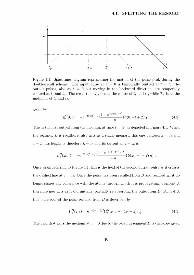
4.1. SPLITTING THE MEMORY
6z
- t
L
z0
¡¡
¡¡
¡¡
¡¡
¡¡
¡¡µ@
@@
@@
@@
@@
@@R
@@
@@@Rtp TA TB t1 t2
Figure 4.1: Spacetime diagram representing the motion of the pulse peak during thedouble-recall scheme. The input pulse at z = 0 is temporally centred at t = tp; theoutput pulses, also at z = 0 but moving in the backward direction, are temporallycentred at t1 and t2. The recall time TA lies at the centre of tp and t1, while TB is at themidpoint of tp and t2.
given by
ΩAb (0, t) = −e−2Γ2(t−TA) 1− e−αz0(1−η)
1− ηΩf(0,−t + 2TA) . (4.2)
This is the first output from the medium, at time t = t1, as depicted in Figure 4.1. When
the segment B is recalled it also acts as a single memory, this one between z = z0 and
z = L. Its length is therefore L− z0 and its output at z = z0 is
ΩBb (z0, t) = −e−2Γ2(t−TB) 1− e−α(L−z0)(1−η)
1− ηΩf(z0,−t + 2TB) .
Once again referring to Figure 4.1, this is the field of the second output pulse as it crosses
the dashed line at z = z0. Once the pulse has been recalled from B and reached z0, it no
longer shares any coherence with the atoms through which it is propagating. Segment A
therefore now acts as it did initially, partially re-absorbing the pulse from B. For z ∈ A
this behaviour of the pulse recalled from B is described by
ΩBb (z, t) = e−α(z0−z)/2ΩB
b [z0, t− n(z0 − z)/c] . (4.3)
The field that exits the medium at z = 0 due to the recall in segment B is therefore given
40
4.1. SPLITTING THE MEMORY
by
ΩBb (0, t) = e−αz0/2ΩB
b (z0, t− nz0/c) (4.4a)
= −e−2Γ2(t−nz0/c−TB) 1− e−α(L−z0)(1−η)
1− ηe−αz0/2Ωf(z0,−t + nz0/c + 2TB) (4.4b)
= −e−2Γ2(t−nz0/c−TB) 1− e−α(L−z0)(1−η)
1− ηe−αz0Ωf(0,−t + 2TB) , (4.4c)
which corresponds to the final output pulse at t = t2 in Figure 4.1.
The principle of superposition allows the total output from the medium to be written
as the sum of ΩAb (0, t) and ΩB
b (0, t). Before doing so though it is useful to consider an
optimization that can be made to minimize the loss that ΩBb experiences as it travels
through segment A.
4.1.1 Optimizing recall efficiency
The pulse recalled from segment B that leaves the medium will be partially re-absorbed
as it travels from z = z0 back to z = 0, as described by (4.3). Note that the absorption
coefficient α depends not only on intrinsic properties of the medium, but is also inversely
proportional to γ, the width of the distribution of detunings present. This width in turn
depends on the strength of the externally-applied electric field, ES, that creates the Stark
shift in the atoms. Therefore, the greater the strength of this electric field the smaller
the value of α.
It has already been assumed that the field ES can be controlled in segments A and B
independently. Therefore if the field strength in A is made sufficiently large before the
recall of B is initiated, re-absorption effects can be safely neglected. That is, the field
recalled from B at a position z ∈ A can now be written simply as
ΩBb (z, t) = ΩB
b [z0, t− n(z0 − z)/c] . (4.5)
41

4.1. SPLITTING THE MEMORY
tp 2TA − tp 2TB − tpTA TB
Inte
nsi
ty
Time
Forward
Backward
δtA
δtB
Figure 4.2: A demonstrative plot of the intensity at z = 0 during the double recall scheme.The first peak, at t = tp, is the input field. The second and third peaks represent scaledcopies of the input pulse reflected about times t = TA and t = TB, respectively.
Under these considerations then, the net effect is that the recalled pulse is given by
ΩBb (0, t) = −e−2Γ2(t−nz0/c−TB) 1− e−α(L−z0)(1−η)
1− ηe−αz0/2Ωf(0,−t + 2TB) . (4.6)
4.1.2 The output pulse
The expression for the total output from the memory can now easily be found as the sum
of the fields resulting from the two recalls. It is convenient to define a scaling factor for
each output pulse. As was the case in Section 3.5, each factor depends on time but can
be well-approximated by the value it takes on at the peak of the corresponding pulse.
That is,
χA := e−2Γ2(TA−tp) 1− e−αz0(1−η)
1− η(4.7)
and
χB := e−2Γ2(TB−tp) 1− e−α(L−z0)(1−η)
1− η. (4.8)
Then, for t > TB,
Ωb(0, t) = −χAΩf(0,−t + 2TA)− χBe−αz0/2e2Γ2nz0/cΩf(0,−t + 2TB) . (4.9)
From this it is easy to see that two time-reversed copies of the input pulse are re-emitted,
with amplitudes that depend on the choice of z0. The first pulse is a scaled reflection
42

4.1. SPLITTING THE MEMORY
of the input about the moment of recall TA. The second pulse is delayed from the first,
being reflected about TB. The storage times of the pulses are defined to be the temporal
separation of each of their peaks from the peak of the input pulse, δtA = 2(TA − tp) and
δtB = 2(TB − tp). This is represented in Figure 4.2.
There are two additional factors to note in the term related to the second pulse. The
first, e−αz0/2, is simply the decrease in amplitude due to the electric field passing through
segment A, an absorbing medium of length z0 (cf. Equation [3.34]). The second, e2Γ2nz0/c,
is slightly more subtle. The scaling factor χB contains a term e−2Γ2(TB−tp) that describes
the decay of the field due to decoherence effects for the time δtB. However, since the
portion of the pulse that was stored in segment B had to travel the length of segment
A twice, a distance 2z0, the time spent propagating through A must be subtracted from
the storage time. The actual time the pulse spent absorbed is thus 2(TB − tp)− 2nz0/c,
and it is this final term which results in the second exponential in (4.9).
4.1.3 Phase difference
As with the single-recall case each output pulse in this scheme will have a phase difference
with respect to the input that depends on its storage time, δϕi = ωLδti. The phase
difference between the two output pulses then depends on the difference in their storage
times,
δϕB − δϕA = ωL (δtB − δtA) . (4.10)
It is useful to express the phase difference modulo 2π. That is, there exists a unique
integer m such that
δϕB − δϕA = 2mπ + δϕ (4.11)
and δϕ ∈ [0, 2π). Let this define the physically relevant phase difference δϕ between the
two output pulses. Conversely, given a desired phase difference one needs only to time
43

4.2. RECALL EFFICIENCY
the recalls appropriately in order to achieve it,
ωL (δtB − δtA) = 2mπ + δϕ =⇒ δtB = δtA +2mπ + δϕ
ωL. (4.12)
4.2 Recall efficiency
As with the the original CRIB protocol, the percentage of total input energy recalled from
the medium is a useful figure of merit for the modified version. Clearly the efficiency of
this new protocol will depend on whether the pulse recalled from segment B interacts with
segment A on its way through. If it does not then the expression for the output pulse
is given by (4.6); otherwise it will be assumed that the absorption coefficient remains
unchanged and the output is given by (4.4c). The only difference between these two
expressions is a factor of e−αz0/2, so they can both be expressed as
ΩBb (0, t) = −e−2Γ2(t−nz0/c−TB) 1− e−α(L−z0)(1−η)
1− ηe−αz0qΩf(0,−t + 2TB) , (4.13)
where q ∈ 1, 1/2 describes whether or not re-absorption occurs. Of course, q could take
on other values if the absorption coefficient of segment A was altered during recall, but
not taken arbitrarily close to zero. However, there is no reason to increase the coefficient
so examining these two cases will place bounds on the expected recall efficiency.
The definitions used in Chapter 3 are still of use, but the output energy must be
re-examined for this new case,
Eb =
∫ ∞
TA
dt |Ωb(0, t)|2 (4.14a)
=
∫ ∞
TA
dt∣∣χAΩf(0,−t + 2TA) + χBe−αz0qe2Γ2nz0/cΩf(0,−t + 2TB)
∣∣2 (4.14b)
= χ2A
∫ ∞
TA
dt |Ωf(0,−t + 2TA)|2 + χ2Be−2αz0qe4Γ2nz0/c
∫ ∞
TA
dt |Ωf(0,−t + 2TB)|2
+ χAχBe−αz0qe2Γ2nz0/c
(∫ ∞
TA
dt Ωf(0,−t + 2TA)Ω∗f (0,−t + 2TB) + c.c.
).
(4.14c)
44

4.2. RECALL EFFICIENCY
The first two integrals are straight-forward to deal with, as will be done soon. The
third integral is worth investigating first however. Note that by defining the variable
s = −t + 2TA the integral can be rewritten as
C[2(TA − TB)] :=
∫ TA
−∞ds Ωf(0, s)Ω
∗f [0, s− 2(TA − TB)] . (4.15)
Since by assumption Ωf(0, s) vanishes for all s > TA the upper limit can be extended
to infinity without affecting the value of the integral. It is then seen that C is the
autocorrelation of Ωf at z = 0. Its value depends explicitly on the duration between the
recalls performed on the two sections A and B. For arbitrary TA and TB this obviously
cannot be evaluated further without knowledge of the specific form of Ωf(0, t). In the
case of interest here though it is assumed that the output pulses are sufficiently far apart
to reasonably define two time bins (as depicted in Figure 4.2). That is, the time between
the pulses is large compared to their widths. In this case, with no further assumptions
on the form of Ωf(0, t), it is clear that C = 0 since there is no moment in time at which
the integrand is non-negligible.
With this knowledge about the third term in the expression for the recalled energy,
and with appropriate changes to the variables of integration, Eb simplifies to
Eb = χ2A
∫ TA
−∞dt |Ωf(0, t)|2 + χ2
Be−2αz0qe4Γ2nz0/c
∫ TB
−∞dt |Ωf(0, t)|2 . (4.16)
Since Ωf(0, t) is assumed to vanish at every time between TA and TB, the upper limit of
the second integral can be reduced to TA so that the total recalled energy can be written
in terms of the input energy (3.56) as,
Eb =(χ2A + χ2
Be−2αz0qe4Γ2nz0/c)Ef . (4.17)
4.2.1 Dependence on z0
The output of this new protocol for generating two smaller pulses from a single larger
one is really a function of z0, the position at which the medium is ‘split’. The efficiency
45

4.2. RECALL EFFICIENCY
of the transformation, equivalent to how much of the input energy is in the output, is
found from (4.17). Using the definitions (4.7) and (4.8) of χA and χB the efficiency is
µ(z0) := e−4Γ2(TA−tp)
(1− e−αz0(1−η)
1− η
)2
+ e−2αz0qe−4Γ2(TB−tp−nz0/c)(
1− e−α(L−z0)(1−η)
1− η
)2
. (4.18)
The value of z0 can range over the full length of the medium, from 0 to L. The limiting
cases are therefore
µ(0) = e−4Γ2(TB−tp)
(1− e−αL(1−η)
1− η
)2
= χ2∣∣T0=TB
(4.19)
and
µ(L) = e−4Γ2(TA−tp)
(1− e−αL(1−η)
1− η
)2
= χ2∣∣T0=TA
. (4.20)
These results agree exactly with what should be expected for them based on the efficiency
of the single-recall scheme, (3.60). Setting z0 = 0 means that segment B comprises the
entire medium, which then behaves as a single-recall memory with recall triggered at time
TB. Similarly z0 = L implies that the whole medium is segment A, so the single-recall
result for triggering at t = TA is recovered.
4.2.2 The ideal case
It has been seen that the effect of a non-zero decay rate is to decrease the amplitude of
the output pulse with increased storage time, and thus to decrease the recall efficiency.
However Γ2 has essentially no impact on the shape of the output pulse. Therefore the
ideal case of Γ2 = 0 will be investigated, though it should be kept in mind that any values
obtained for efficiency or amplitude are merely upper bounds on the physical situation.
In this case the results of the previous subsection simplify significantly. The scaling
coefficients become χA = 1− e−αz0 and χB = 1− e−α(L−z0), and the output pulse is given
46
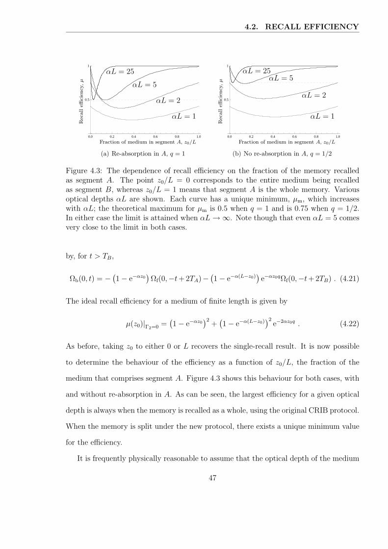
4.2. RECALL EFFICIENCY
0.0 0.2 0.4 0.6 0.8 1.0
0.5
1
Fraction of medium in segment A, z0/L
Rec
all
effici
ency
,µ
αL = 1
αL = 2
αL = 5
αL = 25
(a) Re-absorption in A, q = 1
0.0 0.2 0.4 0.6 0.8 1.0
0.5
1
Fraction of medium in segment A, z0/L
Rec
all
effici
ency
,µ
αL = 1
αL = 2
αL = 5αL = 25
(b) No re-absorption in A, q = 1/2
Figure 4.3: The dependence of recall efficiency on the fraction of the memory recalledas segment A. The point z0/L = 0 corresponds to the entire medium being recalledas segment B, whereas z0/L = 1 means that segment A is the whole memory. Variousoptical depths αL are shown. Each curve has a unique minimum, µm, which increaseswith αL; the theoretical maximum for µm is 0.5 when q = 1 and is 0.75 when q = 1/2.In either case the limit is attained when αL →∞. Note though that even αL = 5 comesvery close to the limit in both cases.
by, for t > TB,
Ωb(0, t) = − (1− e−αz0
)Ωf(0,−t+2TA)− (
1− e−α(L−z0))e−αz0qΩf(0,−t+2TB) . (4.21)
The ideal recall efficiency for a medium of finite length is given by
µ(z0)|Γ2=0 =(1− e−αz0
)2+
(1− e−α(L−z0)
)2e−2αz0q . (4.22)
As before, taking z0 to either 0 or L recovers the single-recall result. It is now possible
to determine the behaviour of the efficiency as a function of z0/L, the fraction of the
medium that comprises segment A. Figure 4.3 shows this behaviour for both cases, with
and without re-absorption in A. As can be seen, the largest efficiency for a given optical
depth is always when the memory is recalled as a whole, using the original CRIB protocol.
When the memory is split under the new protocol, there exists a unique minimum value
for the efficiency.
It is frequently physically reasonable to assume that the optical depth of the medium
47

4.2. RECALL EFFICIENCY
as a whole is sufficiently large that the term e−αL can be neglected. This further simplifies
the recall efficiency, yielding
µ(z0) =(1− e−αz0
)2+ e−2αz0q . (4.23)
It turns out that the position which minimizes this function is the same for both q = 1
and q = 1/2; this position is zm = α−1 ln 2.
Re-absorption, q = 1
When the absorption coefficient of segment A remains constant throughout the protocol
so that the pulse recalled from segment B experiences absorption as it passes through A,
the ideal efficiency (4.22) becomes
µ =(1− e−αz0
)2+ e−2αz0 . (4.24)
When the memory is split at zm the efficiency is µm = 1/2, and the output pulse is given
by
−1
2[Ωf(0,−t + 2TA) + Ωf(0,−t + 2TB)] . (4.25)
The minimum efficiency corresponds to the case of equal-amplitude pulses being recalled
from the memory.
No re-absorption, q = 1/2
Similar analysis when the atoms of segment A are caused to not re-absorb the pulse from
B results in an ideal efficiency of
µ =(1− e−αz0
)2+ e−αz0 . (4.26)
In this case the minimum efficiency is greater; when split at zm the recall efficiency is
µm = 3/4. The amplitude of the pulse recalled from A remains the same, but as expected
the amplitude of the pulse due to B increases; the output pulse is
−1
2Ωf(0,−t + 2TA)− 1√
2Ωf(0,−t + 2TB) . (4.27)
48
4.3. MANIPULATING QUBITS
In this case, obtaining equal-amplitude output pulses requires splitting the medium at
z0 =2
αarcsinh
(1
2
). (4.28)
Since this position is not at zm, the output efficiency is slightly higher in this case,
µ = 3−√5 ≈ 0.764.
4.3 Manipulating qubits
The most commonly used photonic degree of freedom employed to encode information in
photonic qubits propagating through optical fibres is that of arrival time. Polarization
is generally regarded to be the most intuitive choice, and is frequently used to introduce
quantum key distribution via the BB84 protocol. However, standard telecommunications
fibres do not preserve the state of polarization of light propagating through them. This
is why so-called time-bin qubits are a better choice than polarization qubits in most
implementations of quantum key distribution.
4.3.1 Time-bin qubits
The concept of time-bin qubits was introduced in Section 1.3; they will be further mo-
tivated and explored here. By definition the state space of a qubit is two-dimensional.
Therefore any physical system in which one plans to encode a qubit must have a Hilbert
space containing a two-dimensional subspace. If two optical pulses travel sequentially
through air or through an optical fibre, any variations in the index of refraction will af-
fect both equally. Therefore the time separating the two pulse peaks will remain constant
during transmission. This is the motivation behind the definition of time-bin qubits.
Consider a detector that records the time at which a photon is detected. One can
define an arbitrary time as the separation between two states – either the photon arrives
before that time and is ‘early’, or arrives after that time and is ‘late’. Of course, to
49

4.3. MANIPULATING QUBITS
Time
P(fi
nd
photo
n),|ψ|2
-
6
|early〉 |late〉(a) Temporal probability distri-bution for a photon in the state|early〉
Time
P(fi
nd
photo
n),|ψ|2
-
6
|early〉 |late〉(b) A photon in the state |late〉
Time
P(fi
nd
photo
n),|ψ|2
-
6
|early〉 |late〉(c) A superposition state such as1√2
(|early〉+ |late〉)
Figure 4.4: Graphical representation of photons in three different time-bin states. (a)The state |early〉, in which the photon has essentially unit probability of arriving at adetector during the first time bin. (b) When the photon will arrive in the second timebin it is in the state |late〉. (c) A photon prepared in a superposition of |early〉 and |late〉has some non-negligible probability to arrive during either time bin; in this graphic thereis equal probability for both.
be useful for encoding more than a single qubit a window during which the photon is
expected to arrive should be defined, allowing multiple sequential photons to encode
multiple bits. That is, let T be the width of such a window, or bin, and define that if a
photon arrives between t = −T and t = 0 then it is in the state |early〉; arrival between
t = 0 and t = T corresponds to the state |late〉. This system now repeats: For m ∈ Z,
a photon arriving between t = 2(m − 1)T and 2mT is |early〉; one arriving between
t = 2mT and t = 2(m + 1)T is |late〉.
4.3.2 State creation
Under this definition, all photons impinging on the detector must be measured to be
in exactly one of |early〉 and |late〉, assuming either perfect detection efficiency or post-
selection of detection events. Under the further assumption that the photons are known
to have been prepared in states such that there is negligible probability for them to arrive
outside of these two detection windows, this defines a two-dimensional state space for
the photons. To be of practical use one must of course define the time-bin width T to be
longer than the temporal duration of the photonic pulses that will be used.
50

4.3. MANIPULATING QUBITS
It may already be clear that given an input photon in a single well-defined time bin,
the double-recall CRIB protocol allows one to transform the photon into an arbitrary
superposition of |early〉 and |late〉, making the memory device able to act like a variable
beam splitter and phase shifter. This will now be shown explicitly. For simplicity the
ideal case, with Γ2 = 0, αL →∞, and q = 1/2, will be assumed for the remainder of this
chapter. Define
|0〉 := |early〉 and |1〉 := |late〉 , (4.29)
and let the desired output state be given by
a|0〉+ beiϕ|1〉 (4.30)
with a, b, ϕ ∈ R and a2 + b2 = 1. Note that these states define a so-called computational
basis, and that the state |1〉 defined here is unrelated to the atomic energy state employed
in Chapter 2. The two are not used in the same context, so no confusion should arise
from this duplicate definition of the state |1〉. It is also useful at this point to define a
pair of conjugate bases,
B0 := |0〉, |1〉 , and B+ := |+〉, |−〉 , (4.31)
where the states in B+ are defined by
|+〉 :=|0〉+ |1〉√
2, |−〉 :=
|0〉 − |1〉√2
. (4.32)
In order to prepare the state (4.30), one has only to determine the value of z0 that
will produce the amplitude coefficients a and b. The phase ϕ is determined simply by
adding an appropriate delay to TB, as described in Subsection 4.1.3. Note that this delay
is orders of magnitude shorter than the width of a time bin, so that the shift will not
affect the magnitude of a or b.
The normalized recalled state is
−(1− e−αz0) |0〉+ e−αz0/2|1〉√1− e−αz0 + e−2αz0
(4.33)
51
4.3. MANIPULATING QUBITS
from which the coefficients a and b can be read off. Either can be used to determine the
appropriate value of z0. For example,
b = − e−αz0/2√1− e−αz0 + e−2αz0
=⇒ z0 =1
αarccosh
(1 + b2
2b2
). (4.34)
In particular, a qubit initially in the state |1〉 can be transformed into the state |+〉 by
setting b = 1/√
2. One would also set b = 1/√
2 to obtain an output of |−〉, but at the
same time would adjust the phase between the peaks of the two ouput pulses as described
in Subsection 4.1.3.
From these results it is straightforward to see how the effects of either or both of a
beam splitter and a phase shifter can be reproduced from a double-recall CRIB device.
In fact, it is the combination of these two things which can create the state (4.30).
52
Chapter 5
Simulations
The results of the preceding analysis can be supported by numerical integration of the
equations of motion for the system, either in the low-excitation form involving the po-
larization σ or in the more general setting provided by the Bloch equations (2.14). Pro-
gramatically the difference between the two situations is rather minor, so both sets of
equations have been simulated as part of this body of work. The primary purpose of the
simulations is pedagogical, through the pictures they are able to produce of the evolu-
tion of the system within the medium. They also provide the opportunity to investigate
distributions of atomic detunings that are more general than those that fall under the as-
sumptions of the previous chapters. These simulations were written in Matlab [Mat07]
and the source code for the .m file can be found in Appendix A. Based on the strong
similarities between the two sets of code, it was deemed sufficient to include only the
one that simulates σ. This is also the version which was used to generate the majority
of the graphics in this chapter. The results of simulating the different sets of equations
are essentially identical in the case of light pulses equivalent to a few photons in terms
of energy. For example, consider the evolution of the fields presented in Figure 5.1.
In order to facilitate comparisons with and use of experimental data the simulations
make us of SI units. Except where otherwise specified, the values used to create the
results in this chapter were those stated in Table 5.1. The simulations, and indeed the
Maxwell-Bloch equations, determine the evolution of a classical electric field. One can
still make use of them to analyze the single-photon case though; due to the linearity of
the equations of motion, the fields Ωf and Ωb can be interpreted either as classical electric
fields or as the probability amplitudes for a photonic state.
53

010
2030
4050 0
0.2
0.4
0.60
0.2
0.4
0.6
0.8
1
Position,z (cm)
Time,t (ns)
(a) Simulating the absorption ofa single photon based on the fullMaxell-Bloch equations, (5.6)
010
2030
4050 0
0.2
0.4
0.60
0.2
0.4
0.6
0.8
1
Position,z (cm)
Time,t (ns)
(b) Simulating the same initialconditions using the simplifiedMaxwell-Bloch equations, (5.5)
010
2030
4050 0
0.2
0.4
0.60
0.2
0.4
0.6
0.8
1
Position,z (cm)
Time,t (ns)
x10−5
(c) Absolute difference betweenthe two simulation results
Figure 5.1: A comparison of simulation results arising from different forms of theMaxwell-Bloch equations. Note that the vertical scale on the difference plot (c) is fiveorders of magnitude smaller than the scales of the simulation results (a) and (b). It isclear that there is no disadvantage to using the simpler form found in (5.5).
To determine the classical electric field amplitude corresponding to a single photon
the classical and quantum energies may be equated. For the classical case assume that
the pulse is Gaussian in all three spatial dimensions, and has cylindrical symmetry about
the direction of propagation. Let the cross-sectional width of the pulse be given by w;
its width in the z direction is c δt. This results in
E(z) = εE0e−i(ωLt−kz) exp
(− (x2 + y2)
w2
)exp
( −z2
c2δt2
)+ c.c. (5.1)
The task now is to determine the value of E0 in terms of the other known constants
involved. The corresponding magnetic field has magnitude |B| = |E|/c, resulting in the
linear energy density being given by
u(z) =ε0
2
∫ ∞
−∞dx dy
(|E|2 + c2|B|2) = ε0
∫ ∞
−∞dx dy |E|2 . (5.2)
The Gaussian integral over the transverse directions simply evaluates to πw2. The total
energy stored in the field is therefore
U =
∫ ∞
−∞dz u(z) = ε0E
20πw2
∫ ∞
−∞dz e−2z2/c2δt2 = ε0E
20w
2c δt
√π3
2. (5.3)
It is this energy which is equated with the quantum-mechanical expression for the energy
54
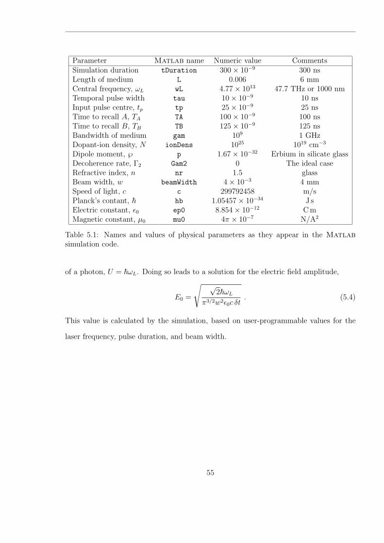
Parameter Matlab name Numeric value CommentsSimulation duration tDuration 300× 10−9 300 nsLength of medium L 0.006 6 mmCentral frequency, ωL wL 4.77× 10¹³ 47.7 THz or 1000 nmTemporal pulse width tau 10× 10−9 10 nsInput pulse centre, tp tp 25× 10−9 25 nsTime to recall A, TA TA 100× 10−9 100 nsTime to recall B, TB TB 125× 10−9 125 nsBandwidth of medium gam 109 1 GHzDopant-ion density, N ionDens 1025 1019 cm−3
Dipole moment, ℘ p 1.67× 10⁻³² Erbium in silicate glassDecoherence rate, Γ2 Gam2 0 The ideal caseRefractive index, n nr 1.5 glassBeam width, w beamWidth 4× 10⁻³ 4 mmSpeed of light, c c 299792458 m/sPlanck’s contant, ~ hb 1.05457× 10⁻³⁴ J sElectric constant, ε0 ep0 8.854× 10⁻¹² C mMagnetic constant, µ0 mu0 4π × 10−7 N/A2
Table 5.1: Names and values of physical parameters as they appear in the Matlabsimulation code.
of a photon, U = ~ωL. Doing so leads to a solution for the electric field amplitude,
E0 =
√ √2~ωL
π3/2w2ε0c δt. (5.4)
This value is calculated by the simulation, based on user-programmable values for the
laser frequency, pulse duration, and beam width.
55

5.1. FORWARD-PROPAGATING MAXWELL-BLOCH SIMULATION
5.1 Forward-propagating Maxwell-Bloch simulation
5.1.1 Co-moving frame
The simulations numerically integrate one of two forms of the Maxwell-Bloch equations.
One of these makes use of σ in the low-excitation limit,
(n
c∂t + ∂z
)Ωf(z, t) = iβ
∫ ∞
−∞d∆ g(∆)σf(z, t, ∆) , (5.5a)
∂tσf(z, t, ∆) = (i∆− Γ2)σf(z, t, ∆) + iΩf(z, t) , (5.5b)
along with the corresponding equations for the backward-moving pulse. The other is
their full form, with decay terms added, given by
(n
c∂t + ∂z
)Ωf(z, t) = iβ
∫ ∞
−∞d∆ g(∆) [r′1(z, t, ∆)− ir′2(z, t, ∆)] , (5.6a)
∂tr′1(z, t, ∆) = ∆r′2(z, t, ∆)− Γ2r
′1 , (5.6b)
∂tr′2(z, t, ∆) = −∆r′1(z, t, ∆) + Ωf(z, t)r
′3(z, t, ∆)− Γ2r
′2 , (5.6c)
∂tr′3(z, t, ∆) = −Ωf(z, t)r
′2(z, t, ∆)− Γ1(1 + r′3) , (5.6d)
as well as the equivalent forms for a pulse propagating in the negative z direction. Here
Γ1 = 1/T1 is the inverse of the natural lifetime of the excited state. The combination of
the two forms results in four sets of coupled differential equations, comprised of a total
of four PDEs and eight ODEs.
A coordinate transformation to a frame moving at the speed of light in the medium
allows the four PDEs ([5.6a], [5.5a], and their backward-moving counterparts) to be recast
as ODEs, without affecting the form of the other eight equations. This procedure is the
same for all four sets of equations, so it suffices to describe the process in detail for one
of them. Specifically, consider (5.5a).
The first step is to define a new set of coordinates, ξ = z and τ = t − nz/c. The
56
5.1. FORWARD-PROPAGATING MAXWELL-BLOCH SIMULATION
paraxial wave operator transforms to this new reference frame as
n
c∂t + ∂z =
n
c
(∂ξ
∂t∂ξ +
∂τ
∂t∂τ
)+
(∂ξ
∂z∂ξ +
∂τ
∂z∂τ
)=
n
c∂τ + ∂ξ − n
c∂τ = ∂ξ , (5.7)
while the partial derivative with respect to time simply becomes
∂t = ∂τ . (5.8)
With the definitions Ωf(ξ, τ) := Ωf(z, t) and σf(ξ, τ, ∆) := σf(z, t, ∆), the equations
(5.5) transform as
∂ξΩf(ξ, τ) = iβ
∫ ∞
−∞d∆ g(∆)σf(ξ, τ, ∆) , (5.9a)
∂τ σf(ξ, τ, ∆) = (i∆− Γ2)σf(ξ, τ, ∆) + iΩf(ξ, τ) . (5.9b)
Given a condition for the initial state of the atoms at some time τ0, σf(ξ, τ0, ∆), and a
boundary condition for the light field over all times at a spatial position ξ0, Ωf(ξ0, τ), the
evolution equation (5.9b) can be solved for the behaviour of the atoms at position ξ0 for
all time, σf(ξ0, τ, ∆). This in turn allows the right-hand side of (5.9a) to be evaluated at
ξ0; now with both Ωf(ξ0, τ) and ∂ξΩf(ξ0, τ) known, an approximation of Ωf(ξ1, τ) can be
made, where ξ1 = ξ0 + δξ represents a position one ‘step’ forward into the medium. This
process can now be repeated to solve for σf(ξ1, τ, ∆) and subsequently Ωf(ξ2, τ), and so
on. In this manner the evolution of the pulse through the medium can be solved over a
given duration and length. A visual depiction of this process can be found in Figure 5.2.
In the case of interest here, the initial condition for the atomic polarization is given
by σf(ξ, τ0, ∆) = 0, since initially all atoms in the medium are in the ground state. The
boundary condition for the light field at ξ = ξ0 represents the pulse entering the medium
that is to be stored.
57
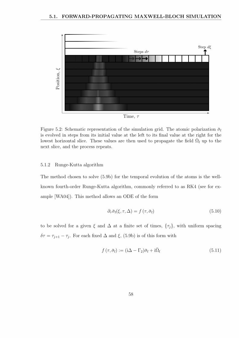
5.1. FORWARD-PROPAGATING MAXWELL-BLOCH SIMULATION
-
6
Time, τ
Pos
itio
n,ξ
Steps dτStep dξ
Figure 5.2: Schematic representation of the simulation grid. The atomic polarization σf
is evolved in steps from its initial value at the left to its final value at the right for thelowest horizontal slice. These values are then used to propagate the field Ωf up to thenext slice, and the process repeats.
5.1.2 Runge-Kutta algorithm
The method chosen to solve (5.9b) for the temporal evolution of the atoms is the well-
known fourth-order Runge-Kutta algorithm, commonly referred to as RK4 (see for ex-
ample [WA04]). This method allows an ODE of the form
∂τ σf(ξ, τ, ∆) = f (τ, σf) (5.10)
to be solved for a given ξ and ∆ at a finite set of times, τj, with uniform spacing
δτ = τj+1 − τj. For each fixed ∆ and ξ, (5.9b) is of this form with
f (τ, σf) := (i∆− Γ2)σf + iΩf (5.11)
58

5.1. FORWARD-PROPAGATING MAXWELL-BLOCH SIMULATION
If the value of σf is known at time τj, then its value at the next time, τj+1, can be found
as follows. First, four coefficients are calculated via
a1 = δτ[(i∆− Γ2)σf(ξ, τj, ∆) + iΩf(ξ, τj)
], (5.12a)
a2 = δτ[(i∆− Γ2)
(σf(ξ, τj, ∆) +
a1
2
)+ iΩf(ξ, τj+1/2)
], (5.12b)
a3 = δτ[(i∆− Γ2)
(σf(ξ, τj, ∆) +
a2
2
)+ iΩf(ξ, τj+1/2)
], (5.12c)
a4 = δτ[(i∆− Γ2) (σf(ξ, τj, ∆) + a3) + iΩf(ξ, τj+1)
], (5.12d)
and then σf is calculated at the next time step as
σf(ξ, τj+1, ∆) = σf(ξ, τj, ∆) +a1 + 2a2 + 2a3 + a4
6. (5.13)
It is assumed that the functional dependence of the input pulse on the time variable τ
is known at the start of the medium, ξ = ξ0. However, in general during the simulation
the values of Ωf will only be known at the discrete times τj. This poses a problem
in determining a2 and a3, which depend on the value of Ωf mid-way between two such
times. As long as δτ is sufficiently small and the input pulse is slowly-varying, as has
been assumed since Section 2.3, this mid-point value can be adequately approximated by
a linear interpolation,
Ωf(ξ, τj+1/2) =Ωf(ξ, τj) + Ωf(ξ, τj+1)
2. (5.14)
In order to be prepared for the integral over ∆ in (5.9a) an array of polarizations
is created, indexed by the detuning ∆ and covering the support of g(∆), which is also
specified at a discrete set of detunings ∆k. The above algorithm is used to evolve each
of these polarizations σf(ξ, τj, ∆k).
5.1.3 Finite difference method
As with the time and detuning domains, the length of the medium is discretized into a
set of points ξi. The desired input pulse is then specified as Ωf(ξ0, τj) for each j in the
59
5.1. FORWARD-PROPAGATING MAXWELL-BLOCH SIMULATION
simulation’s time window. After the atomic polarization has been found for each time at
position ξi, the value of this integral is approximated for each τj by
∫ ∞
−∞d∆ g(∆)σf(ξi, τj, ∆) ≈
∑
k
δ∆ g(∆k)σf(ξi, τj, ∆k) =: δΩ(ξi, τj) , (5.15)
where δ∆ is the uniform spacing between detunings. Since there is no good method
of approximating σf at ξi+1/2 and ξi+1 until Ωf is known at those positions, the RK4
algorithm cannot be used again here.
However, as mentioned at the end of the previous section the pulse envelope Ωf is
assumed to be slowly-varying, in both time and space, so a simpler method of propagating
it to the next position is acceptable. The spatial derivative in (5.9a) is approximated
using the finite difference method, i.e. Newton’s quotient
∂ξΩf(ξi, τj) ≈ Ωf(ξi+1, τj)− Ωf(ξi, τj)
δξ. (5.16)
Equating this to iβ times (5.15) allows the value of the pulse at the next position to be
determined,
Ωf(ξi+1, τj) = Ωf(ξi, τj) + iβ δξ δΩ(ξi, τj) . (5.17)
5.1.4 Algorithm summary – forward direction
It is beneficial to see the steps of the algorithm to simulate the forward direction summa-
rized as a sort of pseudo-code. Let the number of spatial steps comprising the length of
the medium be denoted Mz, and let the number of temporal steps to take in the forward
direction be Mtf. Assuming that all physical quantities are appropriately defined, the
algorithm can be summarized as:
1. Initialize atomic polarizations: Set σf(ξi, τ0, ∆k) = 0 for each i and k
2. Initialize input pulse: Set Ωf(ξ0, τj) = Ωf[0, t(τj)] for each j
3. Define detuning distribution: Set g(∆k) for each k
60
5.1. FORWARD-PROPAGATING MAXWELL-BLOCH SIMULATION
4. Set loop variable i = 0
(a) Set loop variable j = 1
(b) Calculate σf(ξi, τj, ∆k) for each k from (5.13)
(c) Calculate δΩ(ξi, τj) using (5.15) and then Ωf(ξi+1, τj) with (5.17)
(d) Increment j
(e) If j < Mt, repeat from (a)
5. Increment i
6. If i < Mz, repeat from 4
5.1.5 Simulating the Bloch vector
When simulating r′, the Bloch vector in the co-moving frame, equations (5.6) must be
evolved in time instead of (5.5). This is still achieved with the RK4 algorithm but with 12
coefficients to be calculated, the four specified by (5.12) for each of the three components
of the Bloch vector. Written in vector form these coefficients are given by
a1α = δτTαβ(ξi, τj, ∆k)r
′β(ξi, τj, ∆k)− δα3Γ1
, (5.18a)
a2α = δτ
Tαβ(ξi, τj+1/2, ∆k)
[r′β(ξi, τj, ∆k) +
1
2a1α
]− δα3Γ1
, (5.18b)
a3α = δτ
Tαβ(ξi, τj+1/2, ∆k)
[r′β(ξi, τj, ∆k) +
1
2a2α
]− δα3Γ1
, (5.18c)
a4α = δτTαβ(ξi, τj+1/2, ∆k)
[r′β(ξi, τj, ∆k) + a3α
]− δα3Γ1
. (5.18d)
Here α and β are indices that run over 1, 2, 3, and δαβ is the Kronecker delta. Sum-
mation over repeated indices is assumed, and the matrix T = Tαβ is given by
T(ξi, τj, ∆k) =
−Γ2 ∆k 0
−∆k −Γ2 Ωf(ξi, τj)
0 −Ωf(ξi, τj) −Γ1
. (5.19)
61

5.2. BACKWARD-PROPAGATING MAXWELL-BLOCH SIMULATION
As before, the Bloch vector is then evolved via
r′α(ξi, τj+1, ∆k) = r′α(ξi, τj, ∆k) +a1α + 2a2α + 2a3α + a4α
6, (5.20)
and the integral in the source term of the paraxial wave equation is approximated as
∫ ∞
−∞d∆ g(∆) [r′1(ξi, τj, ∆)− ir′2(ξi, τj, ∆)]
≈∑
k
δ∆ g(∆k) [r′1(ξi, τj, ∆k)− ir′2(ξi, τj, ∆k)] =: δΩ(ξi, τj) , (5.21)
In order to simulate the evolution of the Bloch vector instead of the atomic polarization,
there are only two modifications that must be made to the algorithm presented in Sub-
section 5.1.4. One is to calculate r′ instead of σf in Step (b), and the other to calculate
δΩ from (5.21) instead of from (5.15) in Step (c).
5.2 Backward-propagating Maxwell-Bloch simulation
The algorithm described in the previous section simulates the absorption by the medium
of an incoming (i.e. forward-moving) light pulse. In order to simulate the entire CRIB
protocol, it is necessary to use the final state of the medium after the absorption process
as the initial state for a wave propagating in the backward direction. This can be achieved
with the same sort of algorithm as employed in the previous section, but in the backward-
moving reference frame defined by ξ = z and τ = t+nz/c. As in (5.7) the paraxial wave
operator in this new frame is given by
n
c∂t − ∂z = −∂ξ , (5.22)
while the time derivative is unchanged, ∂t = ∂τ . This means that the evolution equations
for σ and r′ also remain unchanged; there is however a slight difference to the paraxial
wave equation (5.9a) that now has a negative sign on the source term,
∂ξΩb(ξ, τ) = −iβ
∫ ∞
−∞d∆ g(∆)σb(ξ, τ, ∆) . (5.23)
62

5.2. BACKWARD-PROPAGATING MAXWELL-BLOCH SIMULATION
However, the simulation is now evolving the field in the backward direction so that when
its value is known at position ξi, the next position at which it must be found is ξi−1 as
opposed to ξi+1. Thus when Newton’s quotient is expressed as
∂ξΩb(ξi, τj) ≈ Ωb(ξi, τj)− Ωb(ξi−1, τj)
δξ, (5.24)
the unknown value of the field is found as
Ωb(ξi−1, τj) = Ωb(ξi, τj) + iβ δξ δΩ(ξi, τj) . (5.25)
Note that despite the opposite signs in the source terms of the forward- and backward-
propagating equations (5.9a) and (5.23), the terms used to calculate the next step of Ω,
provided by the right-hand sides of (5.17) and (5.25), are the same in either case.
5.2.1 Algorithm summary – backward direction
Since the point of simulating the backward direction is to recall the pulse already stored
by the forward simulation, it is assumed that the algorithm in Subsection 5.1.4 has already
been run. With that in mind, let Mtb be the total number of time steps in the whole
simulation, i.e. Mtf plus the number of time steps to take in the backward direction. In
this case, the simulation of the backward direction can be summarized as follows:
1. Initialize polarizations: Set σb(ξi, τMtf, ∆k) = σf(ξi, τMtf
, ∆k) for each i and k
2. Initialize field at end of medium: Set Ωf(ξMz , τj) = 0 for each j
3. Reverse detunings: Set ∆k := −∆k for each k
4. Set position loop variable i = Mz
(a) Set time loop variable j = Mtf + 1
(b) Calculate σb(ξi, τj, ∆k) for each k from (5.13), with ‘b’ subscripts replacing ‘f’
63

5.3. SIMULATING THE PROTOCOL
(c) Calculate δΩ(ξi, τj) from (5.15) with ‘b’ subscripts, and Ωb(ξi−1, τj) with (5.25)
(d) Increment j
(e) If j < Mtb, repeat from (a)
5. Decrement i
6. If i > 0, repeat from 4
5.3 Simulating the protocol
The methods of simulating the evolution of an electric field in a polarizable medium
described in the previous two sections can be combined to simulate various forms of the
CRIB protocol. There is an inherent limitation to them that must always be kept in
mind though: there cannot be in the medium both a forward- and backward-moving
field simultaneously. This does not inhibit simulation of either the standard protocol or
the modified version defined in this work, yet being aware of it is important none the
less.
The methods of the previous sections were used to create the Matlab code found
in Appendix A, which consists primarily of the forward algorithm in Subsection 5.1.4
followed by the backward one of Subsection 5.2.1, along with some commands to visualize
the results. In order to be able to simulate the double-recall CRIB protocol the forward-
direction algorithm must simulate a longer period of time for one part of the medium
than for the rest, which makes the code found in Appendix A slightly more complicated
than merely running Subsections 5.1.4 and 5.2.1 sequentially. The general form however
is as presented therein.
The simulation allows the user to specify in the code the value of b from the target
state (4.30), and from that use (4.34) to calculate the appropriate value of z0 for the
64
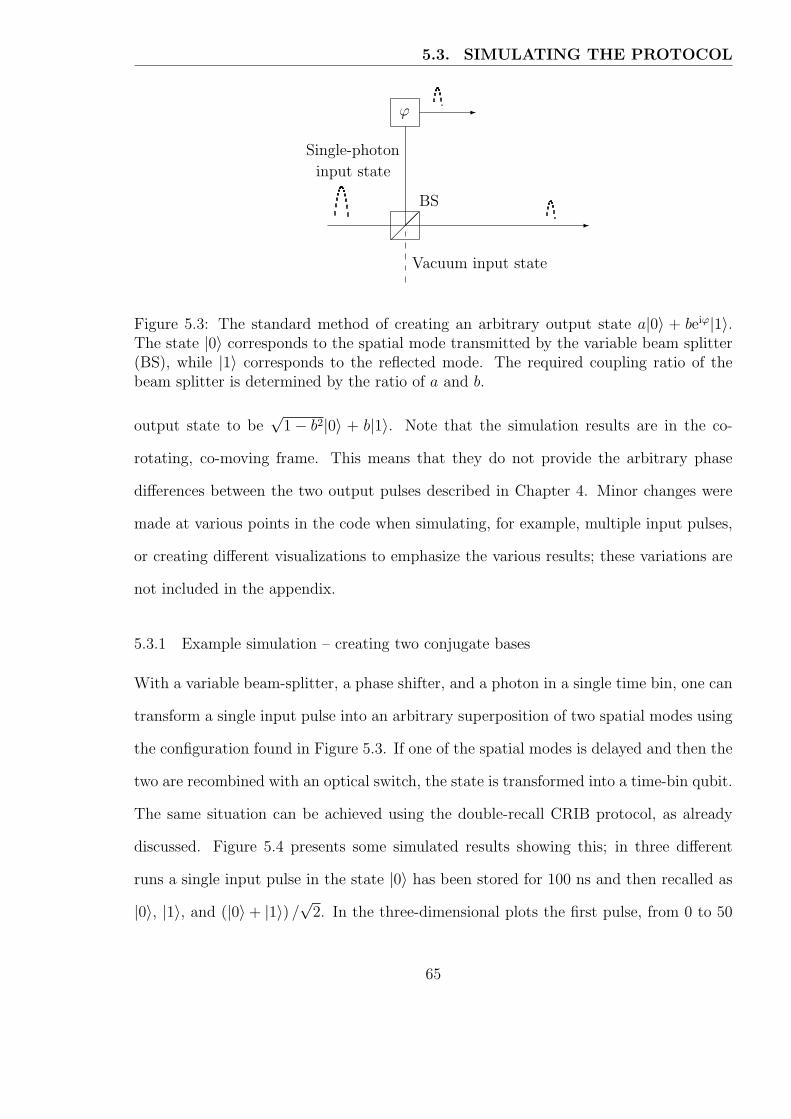
5.3. SIMULATING THE PROTOCOL
¡¡¡ -
-ϕ
Single-photon
input state
Vacuum input state
BS
Figure 5.3: The standard method of creating an arbitrary output state a|0〉 + beiϕ|1〉.The state |0〉 corresponds to the spatial mode transmitted by the variable beam splitter(BS), while |1〉 corresponds to the reflected mode. The required coupling ratio of thebeam splitter is determined by the ratio of a and b.
output state to be√
1− b2|0〉 + b|1〉. Note that the simulation results are in the co-
rotating, co-moving frame. This means that they do not provide the arbitrary phase
differences between the two output pulses described in Chapter 4. Minor changes were
made at various points in the code when simulating, for example, multiple input pulses,
or creating different visualizations to emphasize the various results; these variations are
not included in the appendix.
5.3.1 Example simulation – creating two conjugate bases
With a variable beam-splitter, a phase shifter, and a photon in a single time bin, one can
transform a single input pulse into an arbitrary superposition of two spatial modes using
the configuration found in Figure 5.3. If one of the spatial modes is delayed and then the
two are recombined with an optical switch, the state is transformed into a time-bin qubit.
The same situation can be achieved using the double-recall CRIB protocol, as already
discussed. Figure 5.4 presents some simulated results showing this; in three different
runs a single input pulse in the state |0〉 has been stored for 100 ns and then recalled as
|0〉, |1〉, and (|0〉+ |1〉) /√
2. In the three-dimensional plots the first pulse, from 0 to 50
65

5.3. SIMULATING THE PROTOCOL
0 50 100 150 200 250 0
0.2
0.4
0.6
0
0.2
0.4
0.6
0.8
1
Inte
nsi
ty(a
.u.)
Time, t (ns)
Position,z (cm) 0 50 100 150 200 250
0
0.1
0.2
0.3
0.4
0.5
0.6
0.7
0.8
0.9
1
Inte
nsi
ty(a
.u.)
Time, t (ns)
(a) Recalling the input pulse in the state |0〉
0 50 100 150 200 250 0
0.2
0.4
0.6
0
0.2
0.4
0.6
0.8
1
Inte
nsi
ty(a
.u.)
Time, t (ns)
Position,z (cm) 0 50 100 150 200 250
0
0.1
0.2
0.3
0.4
0.5
0.6
0.7
0.8
0.9
1
Inte
nsi
ty(a
.u.)
Time, t (ns)
(b) Recalling the input pulse in the state |1〉
050
100150
200250 0
0.2
0.4
0.60
0.2
0.4
0.6
0.8
1
Inte
nsi
ty(a
.u.)
Time, t (ns)
Position,z (cm) 50 100 150 200 250
0
0.1
0.2
0.3
0.4
0.5
0.6
0.7
0.8
0.9
1
Inte
nsi
ty(a
.u.)
Time, t (ns)
Input¾ - Storage¾ - Early¾ - Late¾ -
(c) Recalling the input pulse in the superposition state 1√2
(|0〉+ |1〉)
Figure 5.4: Simulating the transformation of a single input pulse in the state |0〉 = |early〉into various output states, using the double-recall CRIB scheme. In each case an inputpulse centred at t = 25 ns propagating in the +z direction is absorbed. (a) Recall wasinitiated from the entire medium at t = 100 ns. (b) Recall was initiated from the entiremedium at t = 125 ns. (c) Recall began in segment A from z = 0 to z = z0 = 0.967 mmat time t = 100 ns, and started in the rest of the medium at t = 125 ns.
66

5.3. SIMULATING THE PROTOCOL
ns, is the input field propagating into and being absorbed by the medium that is 6 mm
long. The light is stored during the period of time from 50 ns to either 150 ns or 200
ns, depending on the simulation. The pulses after t = 150 ns are those recalled from the
medium. Propagating in the negative z direction, they are seen to build up within the
medium before exiting it at z = 0. Note that the second output pulse in Figure 5.4(c)
builds up for a while and then remains constant in amplitude. This starts at the point
that the pulse reaches z0, and is due to the absorption coefficient being negligible in the
first segment at that time.
5.3.2 Interfering two time bins
When working with time-bin qubits, one of course cannot always assume that the input to
a system will be in a single time-bin state. Indeed, it is the ability to have superpositions
of early and late that allows the BB84 protocol to function in the time-bin basis. An
important aspect of BB84 implementations in particular, and qubit manipulations in
general, is the ability to interfere the portions of the photon in different time bins with
each other. Traditionally this is achieved with an unbalanced interferometer, as was seen
in Figure 1.2. With the double-recall CRIB protocol this overlap can also be seen by
timing the recalls appropriately. If the late time bin recalled from segment A coincides
with the early time bin from B, the two fields will be superposed at the memory’s output.
When the phase difference between the two input pulses is zero, as for the state |+〉, the
two will interfere contructively in the central time bin. On the other hand, a phase
difference of π results in destructive interference so that no energy is recalled during
the middle time window. These two statements are easily seen in the simulation results
presented in Figure 5.5.
67

5.3. SIMULATING THE PROTOCOL
0
100
200
300 0
0.2
0.4
0.60
0.2
0.4
0.6
0.8
1
0 50 100 150 200 250 3000
0.1
0.2
0.3
0.4
0.5
0.6
0.7
0.8
0.9
1
(a) Input state: |+〉
0
100
200
300 0
0.2
0.4
0.60
0.2
0.4
0.6
0.8
1
0 50 100 150 200 250 3000
0.1
0.2
0.3
0.4
0.5
0.6
0.7
0.8
0.9
1
(b) Input state: |−〉
Figure 5.5: When the input pulse is in a superposition of two time-bin states, recall canbe timed such that the two input pulses overlap in the output. This can result in (a)constructive or (b) destructive interference.
68

5.3. SIMULATING THE PROTOCOL
50 100 150 200 250 300 350 400 450 500
Inte
nsity
(a.u
.)
Time, t (ns)
Figure 5.6: The effect of non-zero Γ2 on recall efficiency. The same input pulse issent into the medium multiple times, and recalled after various delays. The effect ofΓ2 = 2 × 10⁶ s−1 is easily seen in the decreasing amplitude of the recalled pulses withincreasing storage time.
5.3.3 Simulating decoherence
The expected result for a non-zero rate of decoherence is for the efficiency of the recall
to decrease exponentially with increased storage time. The simulations were written to
include a constant Γ2 in the evolution of the atomic polarization, but set equal to zero by
default. To demonstrate the effect of decoherence, a simulation of the same system was
run repeatedly, changing only the recall time for each run. These results can be found in
Figure 5.6. It can be seen that the pulse width is unaffected, resulting in a reshaping of
the pulse.
To achieve such an obvious decay in the pulse height over less than a microsecond, the
decoherence rate was set to Γ2 = 2× 10⁶ s−1. Such a large rate would have a significant
impact on the output of the double recall scheme, however at the more physical rate of
Γ2 = 105 s−1 the effects of decoherence are negligible over a few tenths of a microsecond.
As can be seen in Figure 5.7, the efficiency of the double recall scheme is practically
unaffected by the lower decoherence rate, whereas not only is the overall efficiency greatly
decreased with the higher rate but the two output pulses are no longer equal in amplitude.
69

5.3. SIMULATING THE PROTOCOL
0 50 100 150 200 250 3000
0.1
0.2
0.3
0.4
0.5
0.6
0.7
0.8
0.9
1
(a) Decoherence rate Γ2 = 105 s−1
0 50 100 150 200 250 3000
0.1
0.2
0.3
0.4
0.5
0.6
0.7
0.8
0.9
1
(b) Decoherence rate Γ2 = 2× 10⁶ s−1
Figure 5.7: In both plots the results of the ideal (Γ2 = 0) case is shown as a lighter line.(a) The total output energy in the case of Γ2 = 105 s−1 is over 96.5% of the recall inthe lossless case. (b) The recalled energy with rapid decoherence is less than 50% of theideal case.
5.3.4 Recall in the forward direction
A user-definable parameter in the code, fwdSim, determines whether or not the simulation
will recall the pulse in the forward direction. When this boolean variable is true, the
entire simulation is run in the forward direction. Figure 5.8 shows the results of two such
simulations. In the first, the whole medium was recalled at a single time, with b = 0. In
this simulation the parameters were set the same as in the creation of Figure 5.4(a). The
amplitude of the output pulse within the medium is proportional to z2e−z, as predicted
by Sangouard et al. [SSAG07]. The shape of this predicted curve can be seen in the
amplitude of the output pulse of Figure 5.8(a).
In the second simulation, z0 was calculated so that b would have been 1/√
2 had
the recall been in the backward direction. This run used the same parameters as the
double-recall simulation presented in 5.4(c). It can be seen that the amplitude of the
second output pulse follows the same general shape as the one in Figure 5.8(a). For the
length of segment A, i.e. from 0 to z0, the first output pulse does as well. However,
as soon as it enters segment B it starts to get re-absorbed, and decays exponentially
70

5.3. SIMULATING THE PROTOCOL
0 50 100 150 200 250 0
0.2
0.4
0.6
0
0.2
0.4
0.6
0.8
1In
tensi
ty(a
.u.)
Time, t (ns)
Position,z (cm)
(a) Single recall in the forward direction
0 50 100 150 200 250 0
0.2
0.4
0.6
0
0.2
0.4
0.6
0.8
1
Inte
nsi
ty(a
.u.)
Time, t (ns)
Position,z (cm)
(b) Double recall in the forward direction
Figure 5.8: Without application of the 2kz phase shift, the pulse continues to travelin the positive z direction when it is recalled. The recalled pulses can be seen to startincreasing in amplitude, before continuing to be absorbed by the medium. Besides notswitching to the backward direction after storage, all other simulation parameters arethe same as those used to create Figure 5.4.
so that there is only negligible output from segment A at z = L. This effect can be
minimized using the same technique as was used to maximize the output efficiency of the
backward-direction double recall. If the pulse is instead recalled from segment B first,
after which the absorption coefficient in that region is made as small as possible, then
when segment A is recalled its output will move through B unhindered. An example
resulting from this setup can be seen in Figure 5.9. While the total energy recalled from
the medium is greater than either case in Figure 5.8, it is still less than the output of the
double-recall backward case of Figure 5.4(c). Furthermore, some of the original energy
is lost due to incomplete absorption of the initial pulse; if the medium is optically dense
enough to absorb the entire input, then it will also re-absorb a significant portion of the
output.
71

5.3. SIMULATING THE PROTOCOL
050100150200250
0
0.1
0.2
0
0.2
0.4
0.6
0.8
1
Inte
nsi
ty(a
.u.)
Time, t (ns)
Position,z (cm)
(a) Intensity within the medium. Note that theviewing angle is different from previous plots.
0 50 100 150 200 2500
0.1
0.2
0.3
0.4
0.5
0.6
0.7
0.8
0.9
1
Inte
nsi
ty(a
.u.)
Time, t (ns)
Input at z = 0¾
Output atz = L
HHHHHj@@R
¡¡
¡¡ª
(b) Plot of the pulse intensity at the two endsof the medium.
Figure 5.9: Simulation results for implementing the double-recall protocol in the forwarddirection with no absorption of the pulse recalled from segment A as it moves throughsegment B. Note that in order for the important features of the three-dimensional plotof intensity to be visible, this plot views the result from a different angle than previousresults; time increases to the left, and the pulse enters at the back and propagates towardthe front.
72

Chapter 6
Concluding remarks
The primary motivation for the present work came from the field of quantum key dis-
tribution, in which quantum memory devices are important for extending arbitrarily the
distance over which QKD can be performed; in this work a new variation to the well-
known quantum memory protocol based on controlled reversible inhomogeneous broad-
ening has been introduced. By treating the storage medium as two separate regions, and
by tailoring the relative lengths of those two sections as well as the times at which recall is
performed in each one, a method has been constructed that allows quantum state storage
to be combined with a beam-splitting operation. For instance, this combination allows
the transformation of a single temporally localized pulse into an arbitrary superposition
of pulses in two distinct time bins. The double-recall scheme allows this transformation to
be performed with nothing more than control of static electric fields, making the method
potentially more stable and simple to implement than the current alternative provided
by interferometers that must be mechanically stabilized to within a small fraction of an
optical wavelength. Of particular importance in the context of experimental QKD is the
fact that this allows the performance of projection measurements onto the bases B0 and
B+, without the need for interferometers to be stabilized over long distances. Important
steps toward this result have been made, as seen in the results of Figure 5.5 that show
constructive and destructive interference at the output of the medium. This corresponds
to one of the output ports of an interferometer. Future directions for expanding the
scope of this work include an investigation into methods for reproducing the results of
the second output port in order to complete the set of measurements required by BB84.
This will provide another use of quantum memory within the realm of QKD.
73

Appendix A
Matlab simulation code
The simulation results presented in Chapter 5 were created with the code listed below,with modification only to parameters as mentioned in the text or to the visualizationcommands employed at the end.
%%%%%%%%%%%%%%%%%%%%%%%%%%%%%%%%%%%%%%%%%%%%%%%%%%%%%%%%%%%%%%%%%%%%%%%%
display([datestr(now,14), ’: Initializing’]);
clear all;
close all;
opengl neverselect; % Solves some graphics-card related crashes
%% Options
fwdSim = false;
b=1/sqrt(2); % Probability amplitude of second output pulse
% All quantities are defined in SI units
tDuration = 300e-9; % Duration of simulation, 300 ns
L = 0.006; % Length of simulated medium, 6 mm
tau = 10e-9; % Temporal width of pulse, 10 ns
wL = 4.77e13; % Central frequency of laser
% Corresponds to 1000 nm wavelength
tp = 25e-9; % Centre of pulse, 25 ns
binSep = 50e-9;
TA = 100e-9; % Time when recall starts in segment A
TB = 125e-9; % Time when recall starts in segment B
gam = 1e9; % Storage bandwidth of medium, 1 GHz
nr = 1.5; % refractive index of medium
c = 299792458; % speed of light
hb = 1.05457e-34; % reduced Planck’s constant, hbar
mu0 = pi*4e-7; % permeability of free space
74
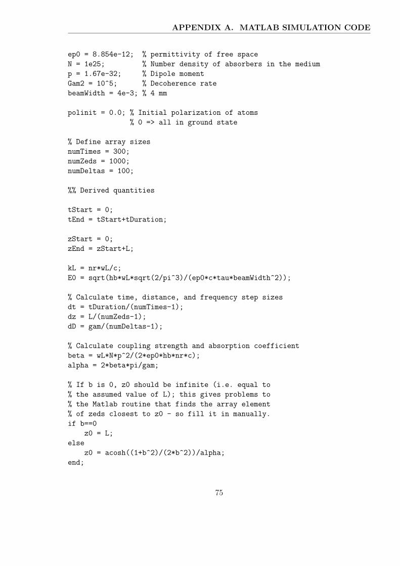
APPENDIX A. MATLAB SIMULATION CODE
ep0 = 8.854e-12; % permittivity of free space
N = 1e25; % Number density of absorbers in the medium
p = 1.67e-32; % Dipole moment
Gam2 = 10^5; % Decoherence rate
beamWidth = 4e-3; % 4 mm
polinit = 0.0; % Initial polarization of atoms
% 0 => all in ground state
% Define array sizes
numTimes = 300;
numZeds = 1000;
numDeltas = 100;
%% Derived quantities
tStart = 0;
tEnd = tStart+tDuration;
zStart = 0;
zEnd = zStart+L;
kL = nr*wL/c;
E0 = sqrt(hb*wL*sqrt(2/pi^3)/(ep0*c*tau*beamWidth^2));
% Calculate time, distance, and frequency step sizes
dt = tDuration/(numTimes-1);
dz = L/(numZeds-1);
dD = gam/(numDeltas-1);
% Calculate coupling strength and absorption coefficient
beta = wL*N*p^2/(2*ep0*hb*nr*c);
alpha = 2*beta*pi/gam;
% If b is 0, z0 should be infinite (i.e. equal to
% the assumed value of L); this gives problems to
% the Matlab routine that finds the array element
% of zeds closest to z0 - so fill it in manually.
if b==0
z0 = L;
else
z0 = acosh((1+b^2)/(2*b^2))/alpha;
end;
75

APPENDIX A. MATLAB SIMULATION CODE
%% Initial conditions
% Create arrays to hold real-world times and positions
times = tStart:dt:tEnd;
zeds = zStart:dz:zEnd;
% Initialize the field to zero everywhere in the simulation domain
Omega = zeros(numZeds,numTimes);
% Define a Gaussian input pulse centred at tp
pulseTimes1 = times - tp;
pulseTimes2 = times - (tp+binSep);
Omega(1,:) = E0*exp(-pulseTimes1.*pulseTimes1/tau^2);
% Define the initial and reversed detunings
posDeltas = (-gam/2):dD:(gam/2);
negDeltas = -posDeltas;
% Create the detuning distribution g(Delta)
g = ones(1,numDeltas)/gam;
%% Find the array elements closest to the desired times and positions
[minDiff, tSwitchA] = min(abs(times-TA));
[minDiff, tSwitchB] = min(abs(times-TB));
[minDiff, zSplit] = min(abs(zeds-z0));
Tm = TA+TB-tp;
[minDiff, tMidPoint] = min(abs(times-Tm));
%% The simulation itself
% An array to save the atomic states after the forward simulation
polsave = zeros(numZeds,numDeltas);
Deltas = posDeltas;
for n=1:numZeds
% Initialize the polarizations at this position
pol = polinit*ones(1,numDeltas);
% The field at the first time step won’t change, unless polarization
76

APPENDIX A. MATLAB SIMULATION CODE
% exists in the medium before the field arrives
if n<numZeds;
%Note that this does nothing in the normal case of polinit=0
dE = i*beta*dD*sum(g.*pol);
Omega(n+1,1) = Omega(n,1) + dE*dz;
end;
% In the section A the detunings are switched at a different time
% than in section B
if n<zSplit
runTime = tSwitchA-1;
else
runTime = tSwitchB-1;
end;
for s=1:runTime
% Determine the current, next, and intermediate values of the
% electric field, needed by the RK4 algorithm
Om = Omega(n,s);
OmNext = Omega(n,s+1);
OmHalf = (Om+OmNext)/2;
% Find the RK coefficients
k1 = dt*((i*Deltas-Gam2).*pol + i*Om);
k2 = dt*((i*Deltas-Gam2).*(pol+k1/2) + i*OmHalf);
k3 = dt*((i*Deltas-Gam2).*(pol+k2/2) + i*OmHalf);
k4 = dt*((i*Deltas-Gam2).*(pol+k3) + i*OmNext);
% Calculate pol(n,s+1) using RK4
pol = pol + (k1 + 2*k2 + 2*k3 + k4)/6;
% Calculate the change in Omega over the next step
dOm = i*beta*dD*sum(g.*pol);
if n<numZeds
Omega(n+1,s+1) = Omega(n,s+1) + dOm*dz;
end;
end; % s-loop (times)
% Save the polarizations at time tSwitchA or tSwitchB
polsave(n,:) = pol;
77

APPENDIX A. MATLAB SIMULATION CODE
% Print a status update occasionally
if mod(n,numZeds/10)==0; display([’z=’,num2str(n)]); end;
end;
% Setup variables that allow the next section of code to
% work in either the forward or backward direction
if fwdSim
first = 1;
last = numZeds;
inc = 1;
else
first = numZeds;
last = 1;
inc = -1;
end;
% Reverse the detunings
Deltas = negDeltas;
% Continue the simulation, in the appropriate direction
for n=first:inc:last
% Restore the polarization state at the current position
% from the the result of the above simulation
pol = polsave(n,:);
% The start time for the current simulation, as well as the order
% in which sections are made transparent, depend on the simulation
% direction.
if n<zSplit
runTime = tSwitchA;
if fwdSim
betaSec2 = beta;
else
betaSec2 = 0;
end;
else
runTime = tSwitchB;
if fwdSim
betaSec2 = 0;
else
betaSec2 = beta;
end;
78

APPENDIX A. MATLAB SIMULATION CODE
end;
if n ~= last;
dE = i*beta*dD*sum(g.*pol);
Omega(n+inc,runTime) = Omega(n,runTime) + dE*dz;
end;
betaUse = beta; % Restore the original value of beta,
% in case 0 was used in the previous interation
for s=runTime:numTimes-1
if s==tMidPoint
betaUse = betaSec2;
end;
Om = Omega(n,s); %*2*p/hb;
OmNext = Omega(n,s+1); %*2*p/hb;
OmHalf = (Om+OmNext)/2;
k1 = dt*((i*Deltas-Gam2).*pol + i*Om);
k2 = dt*((i*Deltas-Gam2).*(pol+k1/2) + i*OmHalf);
k3 = dt*((i*Deltas-Gam2).*(pol+k2/2) + i*OmHalf);
k4 = dt*((i*Deltas-Gam2).*(pol+k3) + i*OmNext);
pol = pol + (k1 + 2*k2 + 2*k3 + k4)/6;
dOm = i*betaUse*dD*sum(g.*pol);
if n ~= last;
Omega(n+inc,s+1) = Omega(n,s+1) + dOm*dz;
end;
end; % s-loop (times)
if mod(n,numZeds/10)==0; display([’z=’,num2str(n)]); end;
end;
display([datestr(now,14), ’: Finished simulation’]);
% The complex field cannot be easily visualized,
% and intensity is what is measured experimentally.
% So, calculated the normalized (to one E0 photon)
% intensity of the field.
79
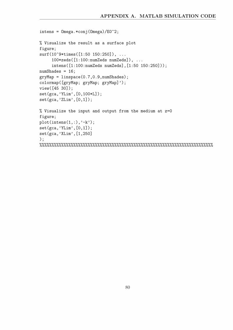
APPENDIX A. MATLAB SIMULATION CODE
intens = Omega.*conj(Omega)/E0^2;
% Visualize the result as a surface plot
figure;
surf(10^9*times([1:50 150:250]), ...
100*zeds([1:100:numZeds numZeds]), ...
intens([1:100:numZeds numZeds],[1:50 150:250]));
numShades = 16;
gryMap = linspace(0.7,0.9,numShades);
colormap([gryMap; gryMap; gryMap]’);
view([45 30]);
set(gca,’YLim’,[0,100*L]);
set(gca,’ZLim’,[0,1]);
% Visualize the input and output from the medium at z=0
figure;
plot(intens(1,:),’-k’);
set(gca,’YLim’,[0,1]);
set(gca,’XLim’,[1,250]
);
%%%%%%%%%%%%%%%%%%%%%%%%%%%%%%%%%%%%%%%%%%%%%%%%%%%%%%%%%%%%%%%%%%%%%%%%
80

Appendix B
Notations and symbols used
|0〉, |1〉 computational basis states from Chapter 4 on (see Page 51)|1〉, |2〉 ground and excited states of a two-level system (see Page 10)
α absorption coefficient (see Pages 26 and 30)β coupling strength between the atoms and light (see Page 16)c speed of light in vacuum, c = 299792458 m/s
c.c. complex conjugateχ scaling factor of the recalled field amplitude (see Page 34)
∂(·) partial derivative with respect to the subscript∆ a detuning, ∆ = ω0 − ωL (see Page 11)
δ(·) Dirac delta distributionδt temporal width of the pulse to be stored (see Page 23)E energy in the light pulse (see Page 36)E electric fieldE pulse envelopeε polarization vectorε0 permittivity of free space, ε0 ≈ 8.854× 10⁻¹² C2/N m2
η constant related to decoherence effects (see Page 31)g(∆) distribution of detunings within the medium (see Page 11)
γ width of absorption profile (see Figure 3.1(c) and Page 3.4)Γ2 decoherence rate in the system (see Page 24)
HA, HI atomic and interaction Hamiltonians (see Pages 10 and 12)~ reduced Planck’s constant, h/2π ≈ 1.055× 10⁻³⁴ J si the complex unit, i2 = −1
Im(·) the imaginary part of the argumentk wavenumber, k = nωL/cL length of the memory medium (see Page 17)µ recall efficiency (see Page 36)
µ12, µ atomic dipole moment and operator (see Page 12)n refractive index or a summation index, dictated by contextN linear density of atomic dipoles (see Page 12)
Ω(z, t) Rabi frequency corresponding to the light field (see Page 16)
Ω(z, ω) Fourier transform of the Rabi frequencyΩ(ξ, τ) Rabi frequency in the co-moving frame (see Page 57)
ω0 transition frequency of a two-level system (see Page 11)ωL central frequency of laser light pulse
ODE, PDE ordinary or partial differential equationP polarization of the medium (see Page 12)℘ projection of light’s polarization on the dipole moment (see Page 13)
81

APPENDIX B. NOTATIONS AND SYMBOLS USED
r, ri Bloch vector, its components (see Page 10)r′, r′i Bloch vector and its components in the co-rotating frame (see Page 14)ρ, ρij density operator, its components ρij = 〈i|ρ|j〉Re(·) the real part of the argument
σ atomic polarization (see Page 12)σ atomic polarization in co-moving frame (see Page 57)t time variableT0 time at which CRIB protocol is initiated (see Page 18)T2 inverse of the medium’s optical linewidth (see Page 23)
TA, TB times at which recall is initiated in segments A and Btp time of the peak of the input pulse (see Page 23)U energy stored in the electric field (see Page 54)w cross-sectional width of the light pulse (see Page 54)z position variablez0 point between z = 0 and z = L at which the memory is split
82

References
[AEW+05] A. Andre, M. D. Eisaman, R. L. Walsworth, A. S. Zibrov, and M. D. Lukin.Quantum control of light using electromagnetically induced transparency.Journal of Physics B, 38:S589–S604, 2005.
[AFK+08] Jurgen Appel, Eden Figueroa, Dmitry Korystov, M. Lobino, and A. I.Lvovsky. Quantum memory for squeezed light. Phys. Rev. Lett., 100:093602,2008.
[AKH66] I. D. Abella, N. A. Kurnit, and S. R. Hartmann. Photon echoes. Phys. Rev.,141(1):391 – 406, January 1966.
[Ale07] Annabel Lucy Alexander. Investigation of Quantum Information Storage inRare Earth Doped Materials. PhD thesis, Australian National University,March 2007.
[ALSM06] A. L. Alexander, J. J. Longdell, M. J. Sellars, and N. B. Manson. Photonechoes produced by switching electric fields. Phys. Rev. Lett., 96:043602,February 2006.
[AML06] Jurgen Appel, K.-P. Marzlin, and A. I. Lvovsky. Raman adiabatic transferof optical states in multilevel atoms. Phys. Rev. A, 73:013804, January 2006.
[BB84] C. H. Bennett and G. Brassard. Quantum cryptography: Public key distri-bution and coin tossing. In Proceedings of IEEE International Conference onComputers, Systems and Signal Processing, pages 175–179, December 1984.
[BB89] Charles H. Bennett and Gilles Brassard. The dawn of a new era in quantumcryptography: The experimental prototype is working! SIGACT News,20:78–83, 1989.
[BBB+92] Charles H. Bennett, Francois Bessette, Gilles Brassard, Louis Salvail, andJohn Smolin. Experimental quantum cryptography. Journal of Cryptology,5(1):3–28, January 1992.
[BBE92] C. H. Bennett, G. Brassard, and A. K. Ekert. Quantum cryptography. Sci-entific American, 267:50–57, October 1992.
[BBM+07] A. D. Boozer, A. Boca, R. Miller, T. E. Northup, and H. J. Kimble. Re-versible state transfer between light and a single trapped atom. Phys. Rev.Lett., 98:193601, May 2007.
[BDCZ98] H.-J. Briegel, W. Dur, J. I. Cirac, and P. Zoller. Quantum repeaters: Therole of imperfect local operations in quantum communication. Phys. Rev.Lett., 81(26):5932–5935, December 1998.
83

REFERENCES
[BGTZ99] J. Brendel, N. Gisin, W. Tittel, and H. Zbinden. Pulsed energy-time en-tangled twin-photon source for quantum communication. Phys. Rev. Lett.,82(12):2594–2597, March 1999.
[BIH91] K.-J. Boller, A. Imamoglu, and S. E. Harris. Observation of electromagneti-cally induced transparency. Phys. Rev. Lett., 66(20):2593–2596, May 1991.
[Blo46] F. Bloch. Nuclear induction. Phys. Rev., 70(7 and 8):460–474, October 1946.
[Cha08] Thierry Chaneliere. Quantum storage investigation in thulium based mate-rials. In Storage and Manipulation of Quantum Information in Optically-Addressed Solids, January 2008.
[CMJ+05] T. Chaneliere, D. N. Matsukevich, S. D. Jenkins, S.-Y. Lan, T. A. B.Kennedy, and A. Kuzmich. Storage and retrieval of single photons trans-mitted between remote quantum memories. Nature, 438:833–836, 2005.
[DLCZ01] L. M. Duan, M. D. Lukin, J. I. Cirac, and P. Zoller. Long-distance quantumcommunication with atomic ensembles and linear optics. Nature, 414:413–418, November 2001.
[Eke91] Artur K. Ekert. Quantum cryptography based on bell’s theorem. Phys. Rev.Lett., 67(6):661–663, August 1991.
[EPR35] A. Einstein, B. Podolsky, and N. Rosen. Can quantum-mechanical descrip-tion of physical reality be considered complete? Physical Review, 47:777–780,May 1935.
[FL00] M. Fleischhauer and M. D. Lukin. Dark-state polaritons in electromagneti-cally induced transparency. Phys. Rev. Lett., 84(22):5094–5097, May 2000.
[HFI90] S. E. Harris, J. E. Field, and A. Imamoglu. Nonlinear optical processes usingelectromagnetically induced transparency. Phys. Rev. Lett., 64(10):1107–1110, March 1990.
[HHDB99] Lene Vestergaard Hau, S. E. Harris, Zachary Dutton, and Cyrus H. Behroozi.Light speed reduction to 17 metres per second in an ultracold atomic gas.Nature, 397:594–598, 1999.
[HLA+08] G. Hetet, J. J. Longdell, A. L. Alexander, P. K. Lam, and M. J. Sellars.Gradient echo quantum memory for light using two-level atoms. Phys. Rev.Lett., 100:023601, January 2008.
[HSSA+06] Sara R. Hastings-Simon, Matthias U. Staudt, Mikael Afzelius, Pascal Baldi,Didier Jaccard, Wolfgang Tittel, and Nicolas Gisin. Controlled stark shifts iner3+-doped crystalline and amorphous waveguides for quantum state storage.Optics Communications, 266(2):716–719, October 2006.
84

REFERENCES
[id 05] id Quantique. Clavis: Plug & Play Quantum Cryptography, id 3000 datasheet,v2.1 edition, 2005.
[KAH64] N. A. Kurnit, I. D. Abella, and S. R. Hartmann. Observation of a photonecho. Phys. Rev. Lett., 13(19):567–568, November 1964.
[KTG+06] B. Kraus, W. Tittel, N. Gisin, M. Nilsson, S. Kroll, and J. I. Cirac. Quantummemory for nonstationary light fields based on controlled reversible inhomo-geneous broadening. Phys. Rev. A, 73:020302(R), 2006.
[LB06] Michel Le Bellac. A Short Introduction to Quantum Information and Quan-tum Computation. Cambridge University Press, 2006.
[LDBH01] Chien Liu, Zachary Dutton, Cyrus H. Behroozi, and Lene Vestergaard Hau.Observation of coherent optical information storage in an atomic mediumusing halted light pulses. Nature, 409:490–493, January 2001.
[Mat07] The MathWorks, Inc. Matlab R2007b: The language of technical com-puting. Software, 1984-2007.
[Mel05] R. S. Meltzer. Spectroscopic Properties of Rare Earths in Optical Materials,chapter 4. Line Broadening Mechanisms and Their Measurement, pages 191–265. Springer Series in Materials Science. Tsunghua University Press andSpringer-Verlag, 2005.
[MK01] S. A. Moiseev and S. Kroll. Complete reconstruction of the quantum stateof a single-photon wave packet absorbed by a doppler-broadened transition.Phys. Rev. Lett., 87(17):173601, October 2001.
[MW95] Leonard Mandel and Emil Wolf. Optical Coherence and Quantum Optics.Cambridge University Press, 1995.
[NC00] Michael A. Nielsen and Isaac L. Chuang. Quantum Computation and Quan-tum Information. Cambridge University Press, 2000.
[NK05] Mattias Nilsson and Stefan Kroll. Solid state quantum memory using com-plete absorption and re-emission of photons by tailored and externally con-trolled inhomogeneous absorption profiles. Optics Communications, 247:393–403, March 2005.
[PFM+01] D. F. Phillips, A. Fleischhauer, A. Mair, R. L. Walsworth, and M. D. Lukin.Storage of light in atomic vapor. Phys. Rev. Lett., 86:783–786, 2001.
[RZBB94] Michael Reck, Anton Zeilinger, Herbert J. Bernstein, and Philip Bertani.Experimental realization of any discrete unitary operator. Phys. Rev. Lett.,73(1):58–61, July 1994.
85

REFERENCES
[SSAG07] Nicolas Sangouard, Christoph Simon, Mikael Afzelius, and Nicolas Gisin.Analysis of a quantum memory for photons based on controlled reversibleinhomogeneous broadening. Phys. Rev. A, 75:032327, March 2007.
[Sta08] Matthias Ulrich Staudt. Probing Coherent Optical Memories in Rare-Earth-Ion-Doped Materials. PhD thesis, Universite de Geneve, April 2008.
[STC+02] Y. Sun, C. W. Thiel, R. L. Cone, R. W. Equall, and R. L. Hutcheson. Recentprogress in developing new rare earth materials for hole burning and coherenttransient applications. Journal of Luminescence, 98:281–287, 2002.
[WA04] Hans J. Weber and George B. Arfken. Essential Mathematical Methods forPhysicists. Elsevier Academic Press, 2004.
[WZ82] W. K. Wootters and W. H. Zurek. A single quantum cannot be cloned.Nature, 299:802–803, October 1982.
86