Bench Measurements and Simulations of Beam Coupling · PDF fileCST Particle Studio® ... Curl-Curl Equation and FIT 17 November 2015 ... 2D impedance solver implemented Open source

17 November 2015 | TU Darmstadt | Fachbereich 18 | Institut Theorie Elektromagnetischer Felder | Uwe Niedermayer | 1

Bench Measurements and Simulations of Beam Coupling Impedance Uwe Niedermayer Institut für Theorie Elektromagnetischer Felder, TU-Darmstadt, Germany CERN Accelerator School on Intensity Limitations in Particle Beams

Maxwell‘s Equations and Particle Beams


Maxwell

Lorentz Force

Update

Interpolate

Self consistent for

PIC Not suitable for

complicated accelerator structures

Wake fields and Beam Coupling Impedance: Divide and Conquer


Maxwell

Update

Wake function or impedance

Electromagnetics

Mechanics

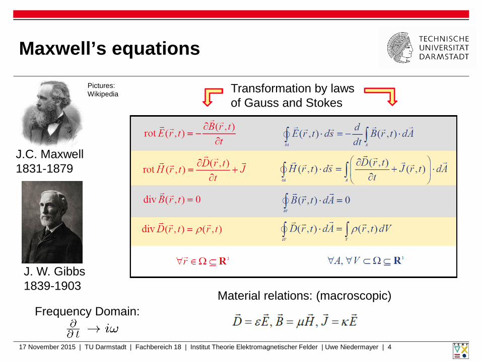
Maxwell’s equations


Frequency Domain:

J.C. Maxwell 1831-1879

J. W. Gibbs 1839-1903

Transformation by laws of Gauss and Stokes

Material relations: (macroscopic)

Pictures: Wikipedia

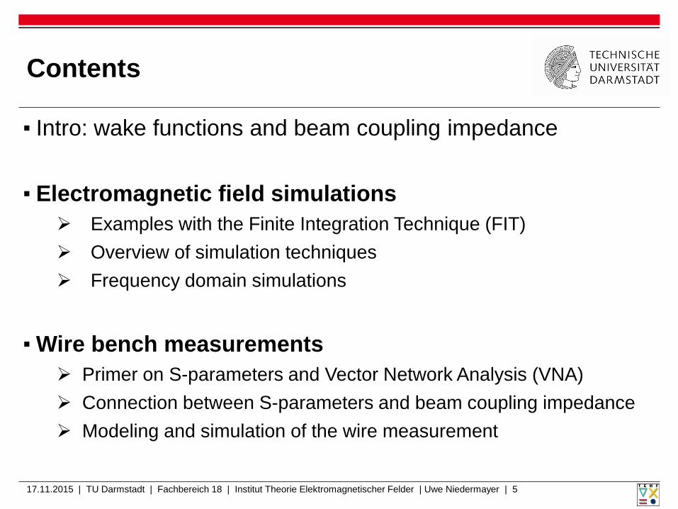
▪ Intro: wake functions and beam coupling impedance

▪ Electromagnetic field simulations Examples with the Finite Integration Technique (FIT) Overview of simulation techniques Frequency domain simulations

▪ Wire bench measurements

Primer on S-parameters and Vector Network Analysis (VNA) Connection between S-parameters and beam coupling impedance Modeling and simulation of the wire measurement

17.11.2015 | TU Darmstadt | Fachbereich 18 | Institut Theorie Elektromagnetischer Felder | Uwe Niedermayer | 5

Contents

Wake Function


▪ Characterizes the accelerator structure ▪ “Kick“ after passage ▪ Green‘s function Wake potential by convolution

▪ Beam Coupling Impedance by Fourier Transform

Source charge Test

charge

Arbitrary accelerator structure

Picture: www.e-hoi.de

Consequences on Beam Dynamics ▪ Can lead to beam instabilities

(both longitudinal and transverse) ▪ Describes beam induced component heating






Contents

Mesh

▪ In general Mesh and Method are independent.

▪ Usually FEM on tetrahedral mesh (unstructured) ▪ Usually FIT/FDTD on hexahedral mesh (structured)


Pictures: Wikipedia

Computational advantages Modeling advantages

Finite Integration Technique (FIT): Grid-Maxwell-Equations


The Grid-Equations represent an EVALUATION of Maxwell‘s equations Therefore they are exact Lecture: Verfahren und Anwendungen der Feldsimulation, TUD

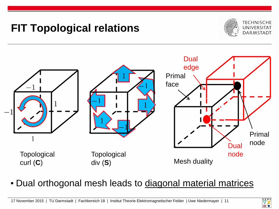
FIT Topological relations

▪ Dual orthogonal mesh leads to diagonal material matrices


Primal node Dual

node

Primal face

Dual edge

Topological curl (C)

Topological div (S) Mesh duality

Leapfrog algorithm and stability

▪ Courant Friedrichs Levy (CFL) stability criterion:

▪ Moreover: grid dispersion, numerical Cherenkov radiation, … 17 November 2015 | TU Darmstadt | Fachbereich 18 | Institut Theorie Elektromagnetischer Felder | Uwe Niedermayer | 13

For equidistant mesh and vacuum

Wake Potential Example (Broadband) Ferrite Ring in Perfectly Electric Conducting (PEC) Pipe


Longitudinal cut

Dispersively lossy ferrite material

10 cm Magnitude of the electric field, logarithmic color scale

Wake potential (convolution of wake function with line density)

Beam line density (a.u.)

CST Particle Studio®

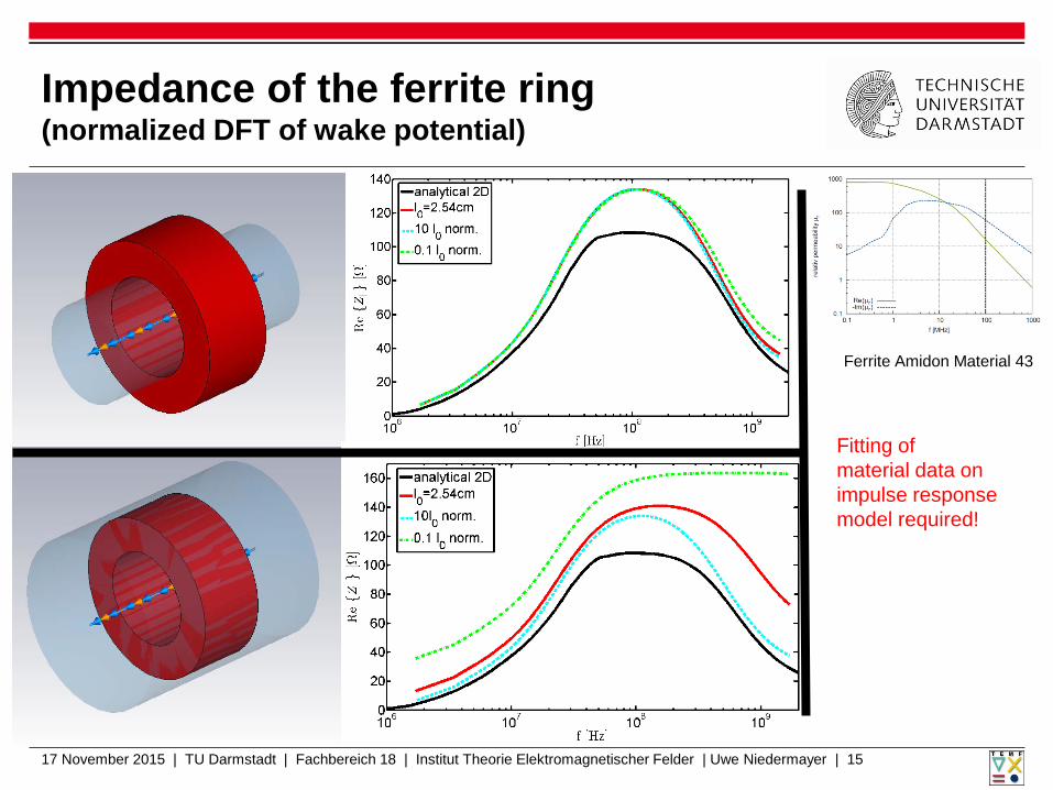
Impedance of the ferrite ring (normalized DFT of wake potential)


Fitting of material data on impulse response model required!

Ferrite Amidon Material 43

Wake Potential Example (Narrowband) Parasitic cavity with 2 gaps (arbitrary…)


Rotationally symmetric

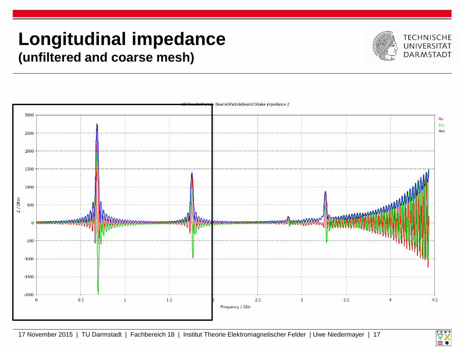
Longitudinal impedance (unfiltered and coarse mesh)


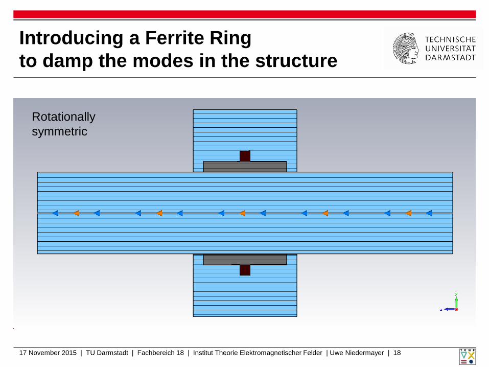
Introducing a Ferrite Ring to damp the modes in the structure



Shifting the ring


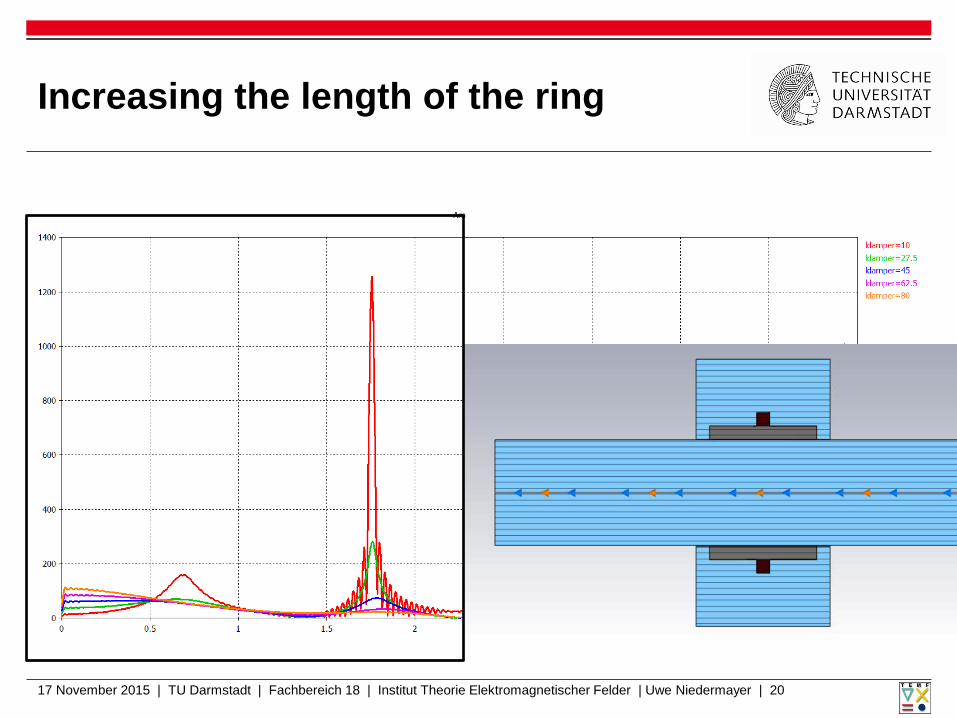
Increasing the length of the ring


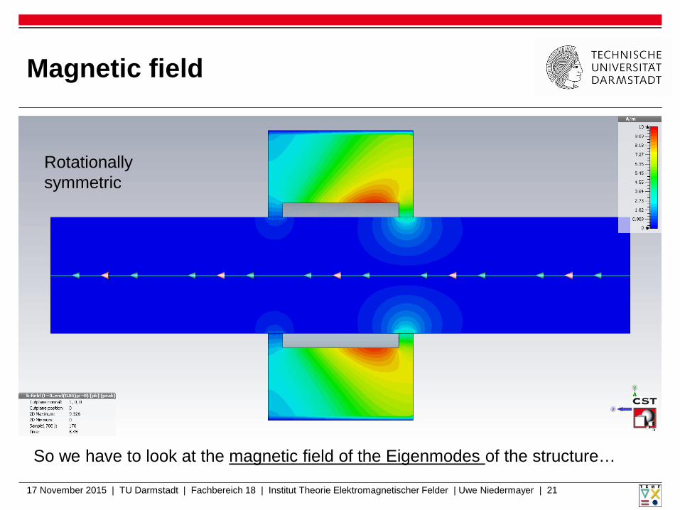
Magnetic field


So we have to look at the magnetic field of the Eigenmodes of the structure…


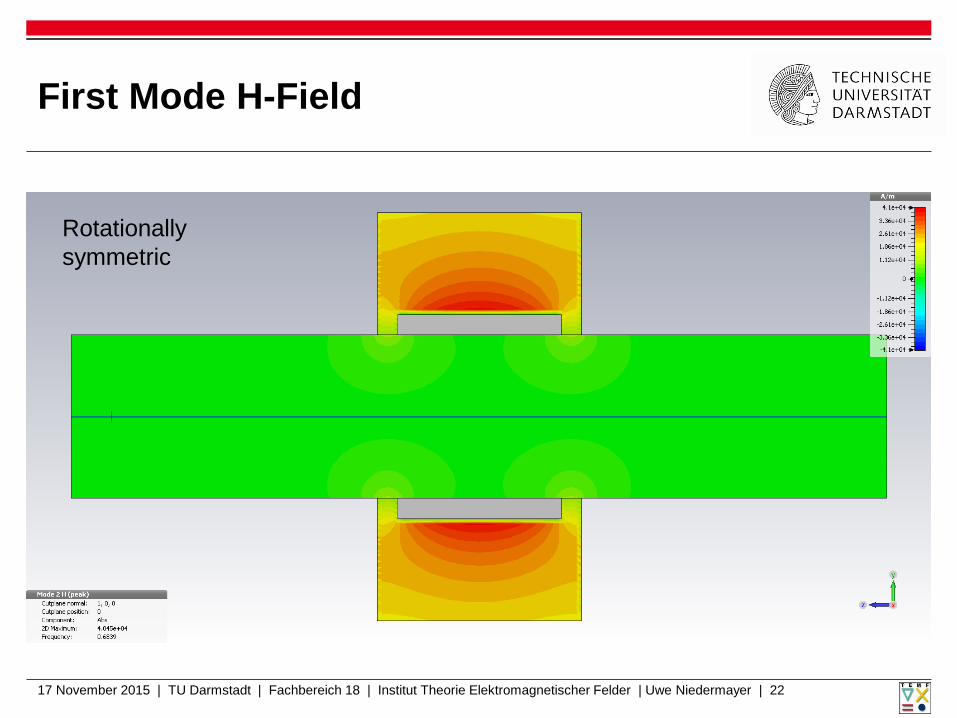
First Mode H-Field



Second Mode H-Field








Contents

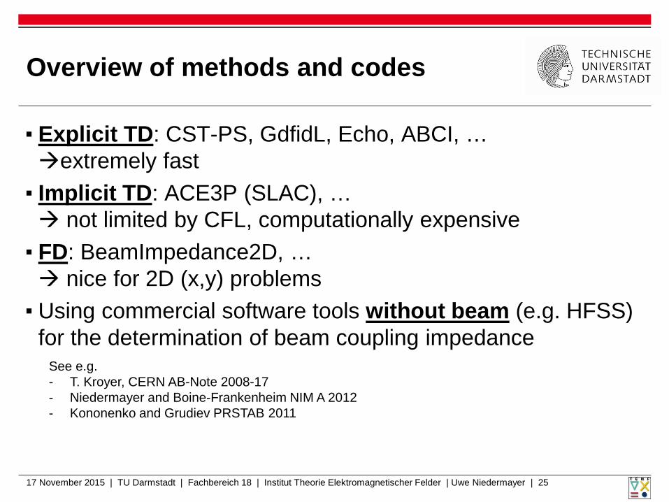
Overview of methods and codes

▪ Explicit TD: CST-PS, GdfidL, Echo, ABCI, … extremely fast

▪ Implicit TD: ACE3P (SLAC), … not limited by CFL, computationally expensive

▪ FD: BeamImpedance2D, … nice for 2D (x,y) problems

▪ Using commercial software tools without beam (e.g. HFSS) for the determination of beam coupling impedance


See e.g. - T. Kroyer, CERN AB-Note 2008-17 - Niedermayer and Boine-Frankenheim NIM A 2012 - Kononenko and Grudiev PRSTAB 2011


Impedance of SIS100 dipole chamber (FD power loss calculation with CST-EMS)

Lowest relevant frequency (specified by Betatron tune)

Longitudinal E-field and wall current for

U.Niedermayer and O. Boine-Frankenheim, Analytical and numerical calculations of resistive wall impedances for thin beam pipe structures at low frequencies, NIM A, 2012

Neclect of beam charge valid at LF and high beam velocity

Dipolar wall current

Properties of Time Domain (TD) and Frequency Domain (FD) Computation

▪ Broadband ▪ Matrix-vector products (cheap) ▪ Commercial / non-commercial

codes available

▪ Limitation at Low Frequency by uncertainty relation and CFL criterion

▪ Difficult for low beam velocity ▪ Difficult for dispersive material


(Explicit-) TD FD (Impedances obtained by DFT)

▪ Arbitrary frequency points ▪ Beam velocity and dispersive

material data are just parameters

▪ Computationally expensive (one ill conditioned linear system of equations (LSE) for each frequency)

▪ Optimized codes not (yet) available

(Impedances obtained directly)






Contents

Defining Sources for Impedance Computation in the Frequency Domain


charged disc

Monopole moment Dipole moment

Longitudinal wake function / impedance Transverse wake function / impedance

displaced source = undisplaced source + dipole moment at the boundary

Beam Coupling Impedance Fourier transform of wake function


Volume integral definition well suited for computation on mesh

Transverse dipolar impedance

Fourier transform

Longitudinal monopolar impedance

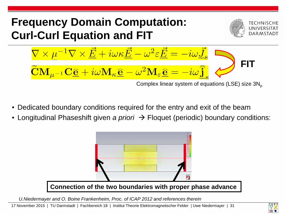
Frequency Domain Computation: Curl-Curl Equation and FIT


FIT

Connection of the two boundaries with proper phase advance

▪ Dedicated boundary conditions required for the entry and exit of the beam ▪ Longitudinal Phaseshift given a priori Floquet (periodic) boundary conditions:

Complex linear system of equations (LSE) size 3Np

U.Niedermayer and O. Boine Frankenheim, Proc. of ICAP 2012 and references therein

Frequency Domain Computation: Curl-Curl Equation and FIT


Complex linear system of equations (LSE) size 3Np

FIT

▪ Dedicated boundary conditions required for the entry and exit of the beam ▪ Longitudinal Phaseshift given a priori Floquet (periodic) boundary conditions:

U.Niedermayer and O. Boine Frankenheim, Proc. of ICAP 2012 and references therein

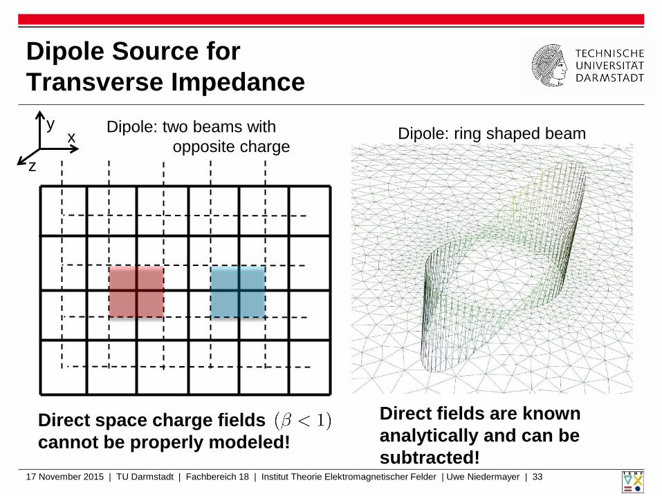
Dipole Source for Transverse Impedance


Direct space charge fields cannot be properly modeled!

Direct fields are known analytically and can be subtracted!

x

z

y Dipole: two beams with opposite charge

Dipole: ring shaped beam

Finite Element Method (FEM)

▪ Very flexible due to unstructured mesh

▪ Discretization of “weak formulation“ ▪ Standard Ritz-Galerkin FEM: trial and test functions are identical

▪ 2D impedance solver implemented ▪ Open source package FEniCS (A. Logg, K. Mardal, G. Wells et al.)

Mesh from Gmsh (C. Geuzaine, J. Remacle) all open source Weak formulation of PDE can be interpreted No complex numbers, can be overcome by coupled function spaces


Discretization of the Electromagnetic Problem in 2D


Discretized by 1st order nodal elements

Discretized by 1st order Nédélec edge elements of the first kind

Split: Longitudinal / Transverse Real / Imaginary

Pic.: P. Jacobsson, Nedelec elements for computational electromagnetics

Helmholtz Split (Domain needs to be simply connected)


“Continuity equation“

solenoidal irrotational

Ritz-Galerkin FEM Discretization


Few (<107) degrees of freedom (dof) in 2D solved with sparse direct solver

U. Niedermayer et al., Space charge and resistive wall impedance computation in the frequency domain using the finite element method, Phys. Rev. –STAB 18, 032001, 2015

Code named “BeamImpedance2D“ (in PYTHON)

Lonitudinal Impedance Examples


A ferrite ring (dispersively lossy material)

Beam of radius a=1cm in perfecly conducting pipe of radius b=4cm

“Longitudinal space charge impedance“

Asymptotes:

Application: Beam Induced Heat Power in SIS 100 transfer kicker magnet


Magnet gap

Dispersive ferrite yoke

Beam

Beam power spectral density Angular revolution frequency

Beam spectrum envelope (a.u.)

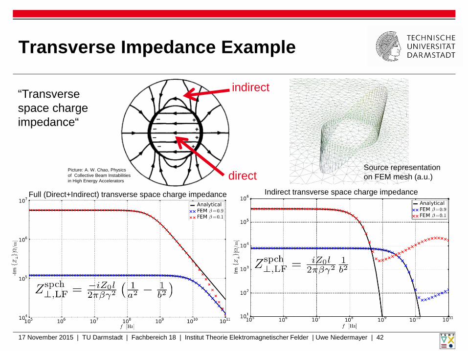
Transverse Impedance Example


Full (Direct+Indirect) transverse space charge impedance

Source representation on FEM mesh (a.u.)

Picture: A. W. Chao, Physics of Collective Beam Instabilities in High Energy Accelerators

Indirect transverse space charge impedance

direct

indirect “Transverse space charge impedance“

Transverse Resistive Wall Impedance: Thin Steel Beam Pipe (idealized SIS-100 pipe)


Resolved wall

Surface impedance boundary condition

d=0.3mm

Thin wall Thick wall






Contents

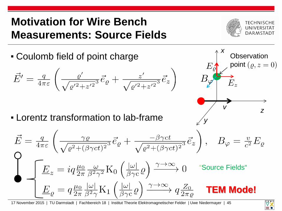
Motivation for Wire Bench Measurements: Source Fields

▪ Coulomb field of point charge


TEM Mode!

v z

x Observation point

y

“Source Fields“

▪ Lorentz transformation to lab-frame

Motivation and History of Wire Bench Measurements


M. Sands, J. Rees, SLAC Report PEP-95, 1974

Beam Bench

• The two setups produce approximately the same image current in the wall • Measurements of loss factors in time domain

It has evolved since 1974…

▪Read as many papers as possible before you start! - F. Caspers, article in the Handbook of Accelerator Physics and Engineering - F. Caspers and A. Mostacci, talk given at ICFA mini workshop on wakefields and impedance, Erice 2014 - G. Nassibian and F. Sacherer, “Methods for Measuring Transverse Coupling Impedances,” Nucl.

Instrum. Meth., vol. 159, no. 6, pp. 21–27, 1978 - H. Hahn and F. Pedersen, “On Coaxial Wire Measurements of the Longitudinal Coupling Impedance,”

BNL Report 78-9, 1978 - T. Kroyer, F. Caspers, and E. Gaxiola, “Longitudinal and Transverse Wire Measurements for the

Evaluation of Impedance Reduction Measures on the MKE Extraction Kickers,” CERN Rep., 2007 - V. Vaccaro, “Coupling Impedance Measurements: An improved wire method,” INFN/TC-94/023, 1994 - E. Jensen, “An improved log-formula for homogeneously distributed impedance,” PS/RF/2000-001 - A. Argan, L. Palumbo, M. R. Masullo, and V. G. Vaccaro, “On the Sands and Rees Measurement

Method of the Longitudinal Coupling Impedance”, Proc. of PAC 8, 1999 - F. Caspers, C. Gonzalez, M. D’yachkov, E. Shaposhnikova, H. Tsutsui, Impedance Measurement Of

The SPS MKE Kicker By Means Of The Coaxial Wire Method, PS/RF/Note 2000-004 - E. Métral, F. Caspers, M. Giovannozzi, A. Grudiev, T. Kroyer, and L. Sermeus, “Kicker impedance

measurements for the future multiturn extraction of the CERN Proton Synchrotron,” in EPAC, Edinburgh, 2006

- Many more, see proceedings







Contents

Wave Amplitudes and Scattering Parameters

▪ Voltage cannot be uniquely defined in RF systems ▪ Thus one defines power flow parameters ai and bi (Unit: sqrt(W))

which are related to the voltage and current in a TEM line by


“Smith Chart“ maps between z and

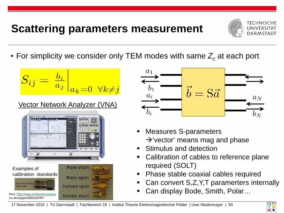
Scattering parameters measurement

▪ For simplicity we consider only TEM modes with same Zc at each port


Vector Network Analyzer (VNA)

Measures S-parameters ‘vector‘ means mag and phase

Stimulus and detection Calibration of cables to reference plane

required (SOLT) Phase stable coaxial cables required Can convert S,Z,Y,T paramerters internally Can display Bode, Smith, Polar…

Examples of calibration standards

Pics: http://www.kirkbymicrowave. co.uk/support/85033/HP/

http://www.kirkbymicrowave/

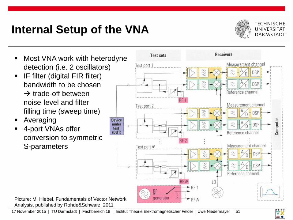
Internal Setup of the VNA


Most VNA work with heterodyne detection (i.e. 2 oscillators)

IF filter (digital FIR filter) bandwidth to be chosen trade-off between noise level and filter filling time (sweep time)

Averaging 4-port VNAs offer

conversion to symmetric S-parameters

Picture: M. Hiebel, Fundamentals of Vector Network Analysis, published by Rohde&Schwarz, 2011

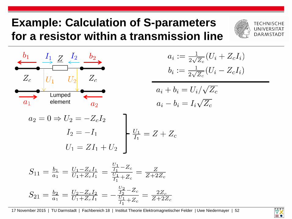
Example: Calculation of S-parameters for a resistor within a transmission line


Lumped element






Contents

Bench Measurements of Broadband Impedances ▪ Measurement in the Frequency Domain

▪ Measure transmission parameter S21

▪ Two fundamental issues

- Corresponds only to scaling by FD simulation - Wire must be thin high characteristic impedance


DUT

REF

VNA

A Priori Distinction between Lumped and Distributed Impedance


DUT

Hahn and Pedersen 1978

Lumped (concentrated) impedance Equally distributed impedance

De-embedded structure: Characteristic Impedance

Distributed Impedance cont‘d


J.Wang and S.Zhang,,” NIM A 459, 2001

Textbook, e.g. Pozar

DUT

Improved Log Formula, Vaccaro et al. 1994

REF

DUT

What if the impedance is neither lumped nor equally distributed?


Log-Formula (Walling et al. 1989)

Requirements for distributed impedance: Requirements for lumped impedance:

U. Niedermayer et al., Analytic modeling, simulation and interpretation of broadband beam coupling impedance bench measurements, Nucl. Instrum. Meth. A 776, 2015 H. Hahn, Validity of coupling impedance bench measurements, PRSTAB 3, 122001, 2000

Mixed Impedance: Log-Formula

‘electrical length‘

Benchmarking the different formulas in 2D (analytical)


(slow) convergence for wire radius

• Beam impedance calculated analytically (multilayer field matching) • S21 calculated from Eigenvalue equation for kz of Quasi-TEM mode

(semi-analytically) U. Niedermayer et al., Analytic modeling, simulation and interpretation of broadband beam coupling impedance bench measurements, Nucl. Instrum. Meth. A 776, 2015


Without reflection correction

Reflection correction • Easy in simulation waveguide ports

• Difficult in reality! Multiple reflections

• Beam impedance from CST Particle Studio (PS)

• S-parameters from CST Microwave Studio (MWS)

With reflection correction

Benchmarking the different formulas in 3D (numerical)

Measurement of the ferrite ring


measurement uncertainty

Large setup

Small setup

Attenuation foam

3.3 cm

L. Eidam

Measurement of Transverse Impedance


▪ S21Z formulas can be linearized

▪ Lumped and distributed impedance do not have to be distinguished

Upper frequency limit due to coil resonance @ approx. 3 MHz

Reasonable measurement results down to 1 kHz Quasi-stationary interpretation required

Twin wire measurement

Expectation by microwave simulation:

L. Eidam

Low frequency measurement of beam pipe transverse impedance


Analytical

Upper frequency limit due to coil resonance @ approx. 3 MHz

Reasonable measurement results down to 1 kHz Quasi-stationary interpretation required

L. Eidam

Summary


▪ Frequency domain beam coupling impedance computation Advantageous for LF, dispersive material, low beam velocity

Direct transverse space charge fields not accurate on structured hex-mesh

Space charge and resistive wall impedance solver in 2D FEM implemented

SIBC allows high frequency since skin depth is not meshed

▪ Bench measurements of broadband impedances Should be cross-checked with RF simulations

A priori knowledge about impedance distribution required for

Medium frequency range

Twin wire method inapplicable at LF by coil method down to 1 kHz

Quasi stationary methods at extremely LF, for both simulation and measurement

Outlook

▪ I will be available the whole week for any questions…

▪ Optimized (parallel) FEM-FD solver in 3D

(PhD position open at TUD)

▪ Optimization of matching networks and conducting bench

measurements (also above cut-off)

(BSc/MSc projects open at GSI and TUD)


The End


Thank you for your attention!

Acknowledgements: - Elias Metral and ICE section at CERN - Fritz Caspers, Manfred Wendt (CERN) - Lewin Eidam, Udo Blell, Oliver Boine-Frankenheim (GSI) - Wolfgang Ackermann, Erion Gjonaj, Ulrich Römer, Herbert De Gersem, Thomas Weiland and

many more… (TEMF)

Any Questions? Please contact me for more references…

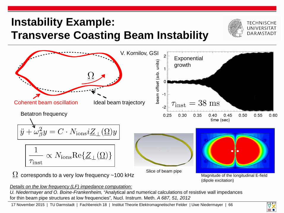
Instability Example: Transverse Coasting Beam Instability


Slice of beam pipe

Details on the low frequency (LF) impedance computation: U. Niedermayer and O. Boine-Frankenheim, “Analytical and numerical calculations of resistive wall impedances for thin beam pipe structures at low frequencies”, Nucl. Instrum. Meth. A 687, 51, 2012

Magnitude of the longitudinal E-field (dipole excitation)

Ideal beam trajectory Coherent beam oscillation

Betatron frequency

V. Kornilov, GSI

corresponds to a very low frequency ~100 kHz

Exponential growth

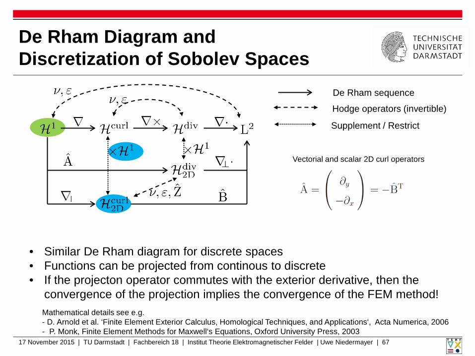
De Rham Diagram and Discretization of Sobolev Spaces


De Rham sequence

Supplement / Restrict

Hodge operators (invertible)

Vectorial and scalar 2D curl operators

• Similar De Rham diagram for discrete spaces • Functions can be projected from continous to discrete • If the projecton operator commutes with the exterior derivative, then the

convergence of the projection implies the convergence of the FEM method! Mathematical details see e.g. - D. Arnold et al. ‘Finite Element Exterior Calculus, Homological Techniques, and Applications‘, Acta Numerica, 2006 - P. Monk, Finite Element Methods for Maxwell‘s Equations, Oxford University Press, 2003

2D Discretization of FCC-hh pipe (similar to LHC pipe)


Gmsh triangular mesh

Design by R. Kersevan, CERN, mesh by T. Egenolf, TU Darmstadt

Meshing the whole structure is required only for extremely low frequency! Otherwise: Surface Impedance Boundary Condition (SIBC)

12mm

18mm

FCC-hh design study: 100TeV c.m., 100km circumf. The first hadron collider where synchrotron radiation losses play significant role

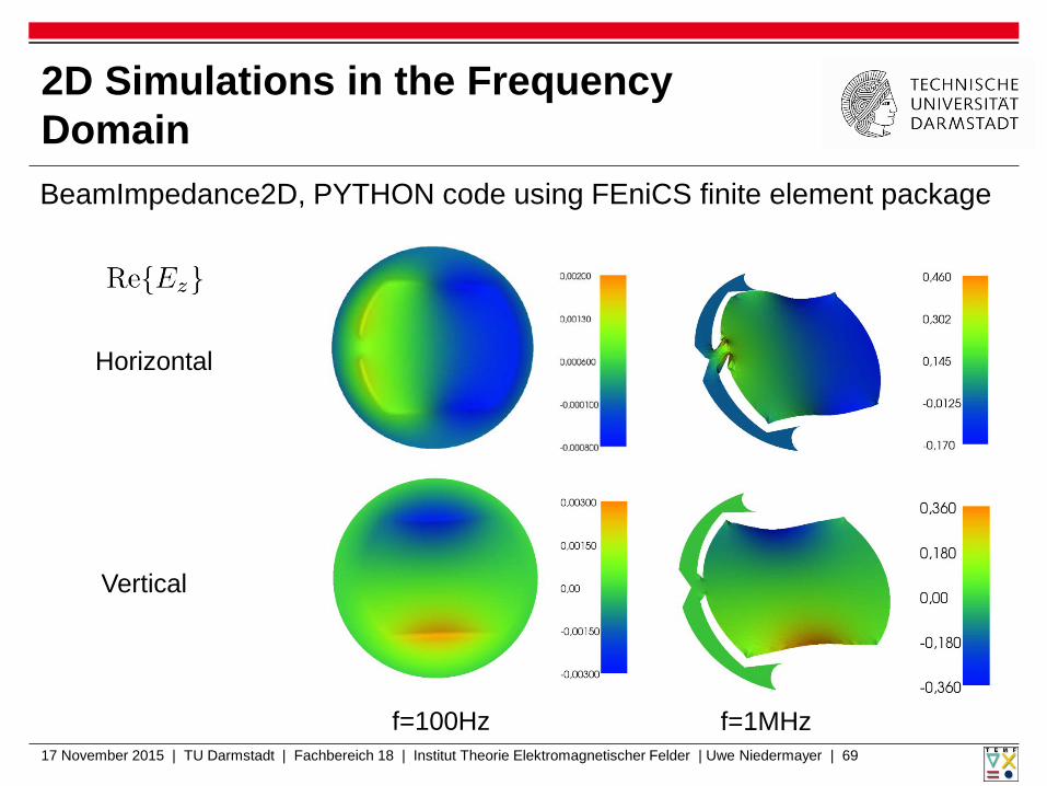
2D Simulations in the Frequency Domain


f=100Hz f=1MHz

Horizontal

Vertical

BeamImpedance2D, PYTHON code using FEniCS finite element package

Penetration Depth

▪ Surface impedance for coated surface


Copper Titanium Vacuum

6.4kHz

Boundary conditions


▪ Natural: Neumann (E-field formulation: Magnetic BC) ▪ Essential: Dirichlet (E-field formulation: Electric BC) ▪ Surface Impedance Boundary Condition (SIBC) ▪ Periodic ▪ Floquet ▪ Open boudary conditions Mur (absorbing BC) Berenger PML (perfectly matched layer)

▪ Waveguide ports Solve 2D eigenvalue problem and connect to 3D structure

▪ Dedicated boundary conditions for particle beams

The Smith Chart


https://upload.wikimedia.org/wikipedia/commons/thumb/d/df/Smith_chart_explanation.svg/2666px-Smith_chart_explanation.svg.png

Documents

Bench Measurements and Simulations of Beam Coupling · PDF fileCST Particle Studio® ... Curl-Curl Equation and FIT 17 November 2015 ... 2D impedance solver implemented Open source