BASIC PROPERTIES OF THE MULTIVARIATE FRACTIONAL BROWNIAN ... · Research supported in part by ANR STARAC grant and a fellowship from Région Rhône-Alpes ... A multivariate extension

BASIC PROPERTIES OF THE MULTIVARIATEFRACTIONAL BROWNIAN MOTION

by

Pierre-Olivier Amblard, Jean-François Coeurjolly, Frédéric Lavancier& Anne Philippe

Abstract. — This paper reviews and extends some recent results on the multivariate frac-tional Brownian motion (mfBm) and its increment process. A characterization of the mfBmthrough its covariance function is obtained. Similarly, the correlation and spectral analysesof the increments are investigated. On the other hand we show that (almost) all mfBm’s maybe reached as the limit of partial sums of (super)linear processes. Finally, an algorithm toperfectly simulate the mfBm is presented and illustrated by some simulations.

Résumé (Propriétés du mouvement brownien fractionnaire multivarié)Cet article constitue une synthèse des propriétés du mouvement brownien fractionnaire

multivarié (mBfm) et de ses accroissements. Di!érentes caractérisations du mBfm sont présen-tées à partir soit de la fonction de covariance, soit de représentations intégrales. Nous étudionsaussi les propriétés temporelles et spectrales du processus des accroissements. D’autre part,nous montrons que (presque) tous les mBfm peuvent être atteints comme la limite (au sensde la convergence faible) des sommes partielles de processus (super)linéaires. Enfin, un algo-rithme de simulation exacte est présenté et quelques simulations illustrent les propriétés dumBfm.

1. Introduction

The fractional Brownian motion is the unique Gaussian self-similar process with station-ary increments. In the seminal paper of Mandelbrot and Van Ness [22], many propertiesof the fBm and its increments are developed (see also [30] for a review of the basic proper-ties). Depending on the scaling factor (called Hurst parameter), the increment process mayexhibit long-range dependence, and is commonly used in modeling physical phenomena.

2000 Mathematics Subject Classification. — 26A16, 28A80, 42C40.Key words and phrases. — Self similarity ; Multivariate process ; Long-range dependence ; Superlinearprocess ; Increment process ; Limit theorem.

Research supported in part by ANR STARAC grant and a fellowship from Région Rhône-Alpes (France)and a Marie-Curie International Outgoing Fellowship from the European Community.Research supported in part by ANR InfoNetComaBrain grant.

2 AMBLARD, COEURJOLLY, LAVANCIER & PHILIPPE

However in many fields of applications (e.g. neuroscience, economy, sociology, physics,etc), multivariate measurements are performed and they involve specific properties such asfractality, long-range dependence, self-similarity, etc. Examples can be found in economictime series (see [11], [14], [15]), genetic sequences [2], multipoint velocity measurementsin turbulence, functional Magnetic Resonance Imaging of several regions of the brain [1].

It seems therefore natural to extend the fBm to a multivariate framework. Recently, thisquestion has been investigated in [20, 19, 5]. The aim of this paper is to summarize andto complete some of these advances on the multivariate fractional Brownian motion andits increments. A multivariate extension of the fractional Brownian motion can be statedas follows :

Definition 1. — A Multivariate fractional Brownian motion (p-mfBm or mfBm) withparameter H ! (0, 1)p is a p-multivariate process satisfying the three following properties

– Gaussianity,– Self-similarity with parameter H ! (0, 1)p,– Stationarity of the increments.

Here, self-similarity has to be understood as joint self-similarity. More formally, we usethe following definition.

Definition 2. — A multivariate process (X(t) = (X1(t), · · · , Xp(t)))t!R is said self-similar if there exists a vector H = (H1, · · · , Hp) ! (0, 1)p such that for any ! > 0,

(1) (X1(!t), · · · , Xp(!t)))t!Rfidi=!!H1X1(t), · · · ,!HpXp(t)

"t!R,

where fidi= denotes the equality of finite-dimensional distributions. The parameter H is called

the self-similarity parameter.

This definition can be viewed as a particular case of operator self-similar processes bytaking diagonal operators (see [12, 16, 17, 21]).

Note that, as in the univariate case [18], the Lamperti transformation induces anisometry between the self-similar and the stationary multivariate processes. Indeed,from Definition 2, it is not di!cult to check that (Y (t))t!R is a p-multivariate stationaryprocess if and only if there exists H ! (0, 1)p such that its Lamperti transformation(tH1Y1(log(t)), . . . , tHpYp(log(t)))t!R is a p-multivariate self-similar process.

The paper is organized as follows. In Section 2, we study the covariance structure ofthe mfBm and its increments. The cross-covariance and the cross-spectral density of theincrements lead to interesting long-memory type properties. Section 3 contains the timedomain as well as the spectral domain stochastic integral representations of the mfBm.Thanks to these results we obtain a characterization of the mfBm through its covariancematrix function. Section 4 is devoted to limit theorems, the mfBm is obtained as the limit ofpartial sums of linear processes. Finally, we discuss in Section 5 the problem of simulating

BASIC PROPERTIES OF THE MULTIVARIATE FRACTIONAL BROWNIAN MOTION 3

sample paths of the mfBm. We propose to use the Wood and Chan’s algorithm [32]well adapted to generate multivariate stationary Gaussian random fields with prescribedcovariance matrix function.

2. Dependence structure of the mfBm and of its increments

2.1. Covariance function of the mfBm. — In this part, we present the form of thecovariance matrix of the mfBm.

Firstly, as each component is a fractional brownian motion, the covariance function ofthe i-th component is well-known and we have

(2) EXi(s)Xi(t) ="2i

2

#|s|2Hi + |t|2Hi " |t" s|2Hi

$.

with "2i := var(Xi(1)). The cross covariances are given in the following proposition.

Proposition 3 (Lavancier et al. [20]). — The cross covariances of the mfBm satisfythe following representation, for all (i, j) ! {1, . . . , p}2, i #= j,

1. If Hi+Hj #= 1, there exists (#i,j, $i,j) ! ["1, 1]$R with #i,j = #j,i = corr(Xi(1), Xj(1))and $i,j = "$j,i such that

(3) EXi(s)Xj(t) ="i"j2

#(#i,j + $i,jsign(s))|s|Hi+Hj + (#i,j " $i,jsign(t))|t|Hi+Hj

"(#i,j " $i,jsign(t" s))|t" s|Hi+Hj$.

2. If Hi+Hj = 1, there exists (#i,j, $i,j) ! ["1, 1]$R with #i,j = #j,i = corr(Xi(1), Xj(1))and $i,j = "$j,i such that

(4)EXi(s)Xj(t) =

"i"j2

{#i,j(|s|+ |t|" |s" t|) + $i,j(t log |t|" s log |s|" (t" s) log |t" s|)} .

Proof. — Under some conditions of regularity, Lavancier et al. [20] actually prove thatProposition 3 is true for any L2 self-similar multivariate process with stationary incre-ments. The form of cross covariances is obtained as the unique solution of a functionalequation. Formulae (3) and (4) correspond to expressions given in [20] after the followingreparameterization : #i,j = (ci,j + cj,i)/2 and $i,j = (ci,j " cj,i)/2 where ci,j and cj,i arise in[20].

Remark 1. — Extending the definition of parameters #i,j, #i,j, $i,j, $i,j to the case i = j,we have #i,i = #i,i = 1 and $i,i = $i,i = 0, so that (2) coincides with (3) and (4).

Remark 2. — The constraints on coe!cients #i,j, #i,j, $i,j, $i,j are necessary but not su!-cient conditions to ensure that the functions defined by (3) and (4) are covariance functions.This problem will be discussed in Section 3.4.


Remark 3. — Note that coe!cients #i,j, #i,j, $i,j, $i,j depend on the parameters (Hi, Hj).Assuming the continuity of the cross covariances function with respect to the parameters(Hi, Hj), the expression (4) can be deduced from (3) by taking the limit as Hi +Hj tendsto 1, noting that ((s + 1)H " sH " 1)/(1 " H) % s log |s| " (s + 1) log |s + 1| as H % 1.We obtain the following relations between the coe!cients : as Hi +Hj % 1

#i,j & #i,j and (1"Hi "Hj)$i,j & $i,j.

This convergence result can suggest a reparameterization of coe!cients $i,j in (1 " Hi "Hj)$i,j.

2.2. The increments process. — This part aims at exploring the covariance structureof the increments of size % of a multivariate fractional Brownian motion given by Defini-tion 1. Let !!X = (X(t+ %)"X(t))t!R denotes the increment process of the multivariatefractional Brownian motion of size % and let !!Xi be its i-th component.

Let &i,j(h, %) = E!!Xi(t)!!Xj(t + h) denotes the cross-covariance of the increments ofsize % of the components i and j. Let us introduce the function wi,j(h) given by

(5) wi,j(h) =

%(#i,j " $i,jsign(h))|h|Hi+Hj if Hi +Hj #= 1,#i,j|h|+ $i,jh log |h| if Hi +Hj = 1.

Then from Proposition 3, we deduce that &i,j(h, %) is given by

(6) &i,j(h, %) ="i"j2

&wi,j(h" %)" 2wi,j(h) + wi,j(h+ %)

'.

Now, let us present the asymptotic behaviour of the cross-covariance function.

Proposition 4. — As |h| % +', we have for any % > 0

(7) &i,j(h, %) & "i"j%2|h|Hi+Hj"2'i,j(sign(h)),

with

(8) 'i,j(sign(h)) =

%(#i,j " $i,jsign(h))(Hi +Hj)(Hi +Hj " 1) if Hi +Hj #= 1,$i,jsign(h) if Hi +Hj = 1.

Proof. — Let ( = Hi + Hj. Let us choose h, such that |h| ( %, which ensures thatsign(h" %) = sign(h) = sign(h+ %). When ( #= 1, this allows us to write

&i,j(h, %) ="i"j2

|h|" (#i,j " $i,jsign(h))B(h),

with B(h) =!1" !

h

"" " 2 +!1 + !

h

"" & ((( " 1)%2h"2, as |h| % +'. When ( = 1 and|h| ( %, &i,j(h, %) reduces to

&i,j(h, %) ="i"j2$i,jB(h) with B(h) =

&(h" %) log

&1" %

h

'+ (h+ %) log

&1 +

%

h

''.


Using the expansion of log(1 ± x) as x % 0 leads to B(h) & %2|h|"1 as |h| % +', whichimplies the result.

Proposition 4 and (6) lead to the following important remarks on the dependence struc-ture. For i #= j and Hi +Hj #= 1 :

– If the two fractional Gaussian noises are short-range dependent (i.e. Hi < 1/2 andHj < 1/2) then they are either short-range interdependent if #i,j #= 0 or $i,j #= 0, orindependent if #i,j = $i,j = 0.

– If the two fractional Gaussian noises are long-range dependent (i.e. Hi > 1/2 andHj > 1/2) then they are either long-range interdependent if #i,j #= 0 or $i,j #= 0, orindependent if #i,j = $i,j = 0. This confirms the dichotomy principle observed in [12].

– In the other cases, the two fractional Gaussian noises can be short-range interdepen-dent if #i,j #= 0 or $i,j #= 0 and Hi +Hj < 1, long-range interdependent if #i,j #= 0 or$i,j #= 0 and Hi +Hj > 1 or independent if #i,j = $i,j = 0.

Moreover, note that when Hi+Hj = 1, whatever the nature of the two fractional Gaussiannoises (i.e. short-range or long-range dependent, or even independent), they are eitherlong-range interdependent if $i,j #= 0 or independent if $i,j = 0.

The following result characterizes the spectral nature of the increments of a mfBm.

Proposition 5 (Coeurjolly et al. [5]). — Let Si,j(·, %) be the (cross)-spectral density ofthe increments of size % of the components i and j, i.e. the Fourier transform of &i,j(·, %)

Si,j(), %) =1

2*

(

Re"ih#&i,j(h, %) dh =: FT (&i,j(·, %)).

(i) For all i, j and for all Hi, Hj, we have

(9) Si,j(), %) ="i"j*

"(Hi +Hj + 1)1" cos()%)

|)|Hi+Hj+1$ +i,j(sign())),

where(10)

+i,j(sign())) =

%#i,j sin

!$2 (Hi +Hj)

"" i$i,jsign()) cos

!$2 (Hi +Hj)

"if Hi +Hj #= 1,

#i,j " i$2 $i,jsign()) if Hi +Hj = 1.

(ii) For any fixed %, when Hi +Hj #= 1 then we have, as ) % 0,(11)

))Si,j(), %))) & "i"j

2*"(Hi +Hj + 1)%2

*#2i,j sin

!$2 (Hi +Hj)

"2+ $2i,j cos

!$2 (Hi +Hj)

"2+1/2

|)|Hi+Hj"1.

(iii) Moreover, when Hi +Hj #= 1, the coherence function between the two componentsi and j satisfies, for all )


Ci,j(), %) :=|Si,j(), %)|2

Si,i(), %)Sj,j(), %)

="(Hi +Hj + 1)2

"(2Hi + 1)"(2Hj + 1)

#2i,j sin!$2 (Hi +Hj)

"2+ $2i,j cos

!$2 (Hi +Hj)

"2

sin(*Hi) sin(*Hj).(12)

(iv) When Hi + Hj = 1, (11) and (12) hold, replacing #2i,j sin!$2 (Hi +Hj)

"2+

$2i,j cos!$2 (Hi +Hj)

"2 by #2i,j + $2

4 $2i,j.

Proof. — The proof is essentially based on the fact that in the generalized function sense,for ( > "1,

FT (|h|") = " 1

*"(( + 1) sin

**2(+|)|"""1,

FT (h"+) =

1

2*"(( + 1)e"isign(#)!2 ("+1)|)|"""1,

FT (h"") =

1

2*"(( + 1)eisign(#)

!2 ("+1)|)|"""1,

FT (h log |h|) = isign())

2)2.

See [5] for more details.

Remark 4. — From this proposition, we retrieve the same properties of dependence andinterdependence of Xi and Xj as stated after Proposition 4.

2.3. Time reversibility. — A stochastic process is said to be time reversible if X(t) =X("t) for all t. As shows in [12], this is equivalent for zero-mean multivariate Gaussianstationary processes to EXi(t)Xj(s) = EXi(s)Xj(t) for s, t ! R or that the cross covarianceof the increments satisfies &i,j(h, %) = &i,j("h, %) for h ! R. The following propositioncharacterizes this property.

Proposition 6. — A mfBm is time reversible if and only if $i,j = 0 (or $i,j = 0) for alli, j = 1, . . . , p.

Proof. — If $i,j = 0 (or $i,j = 0), &i,j(h, %) is proportional to the covariance of a fractionalGaussian noise with Hurst parameter (Hi+Hj)/2 and is therefore symmetric. Let us provethe converse. Let ( = Hi +Hj, then

&i,j(h, %)" &i,j("h, %) = "i"j$%

"$i,j (sign(h" %)|h" %|" + 2sign(h)|h|" " sign(h+ %)|h+ %|") if ( #= 1,$i,j ((h" %) log |h" %|" 2h log |h|+ (h+ %) log |h+ %|) if ( = 1.

Assuming &i,j(h, %)" &i,j("h, %) equals zero for all h leads to $i,j = 0 (or $i,j = 0).


Remark 5. — This result can also be viewed from a spectral point view. The time re-versibility of a mfBm is equivalent to the fact that the spectral density matrix is real. Using(9), this implies $i,j = 0 (or $i,j = 0).

3. Integral representation

3.1. Spectral representation. — The following proposition contains the spectral rep-resentation of mfBm. This representation will be especially useful to obtain a conditioneasy to verify which ensures that the functions defined by (3) and (4) are covariance func-tions.

Theorem 7 (Didier and Pipiras, [12]). — Let (X(t))t!R be a mfBm with parameter(H1, · · · , Hp) ! (0, 1)p. Then there exists a p$ p complex matrix A such that each compo-nent admits the following representation

(13) Xi(t) =p,

j=1

(eitx " 1

ix(Aijx

"Hi+1/2+ + Aijx

"Hi+1/2" )Bj( dx),

where for all j = 1, . . . , p, Bj is a Gaussian complex measure such that Bj = Bj,1 +iBj,2 with Bj,1(x) = Bj,1("x), Bj,2(x) = "Bj,2(x), Bj,1 and Bj,2 are independent andE(Bj,i( dx)Bj,i( dx)#) = dx, i = 1, 2.

Conversely, any p-multivariate process satisfying (13) is a mfBm process.

Proof. — This representation is deduced from the general spectral representation of oper-ator fractional Brownian motions obtained in [12]. By denoting "H+1/2 := diag("H1 +1/2, · · · ,"Hp + 1/2) we have indeed

(14) X(t) =

(eitx " 1

ix(x"H+1/2

+ A+ x"H+1/2" A)B( dx).

Any mfBm having representation (13) has a covariance function as in Proposition 3.The coe!cients #i,j, $i,j, #i,j and $i,j involved in (3) and (4) satisfy

(15) (AA$)i,j ="i"j2*

"(Hi +Hj + 1)+i,j(1),

where +i,j is given in (10) and where A$ is the transpose matrix of A. This relation isobtained by identification of the spectral matrix of the increments deduced on the onehand from (13) and provided on the other hand in Proposition 5.

Given (13), relation (15) provides easily the coe!cients #i,j, $i,j, #i,j and $i,j which definethe covariance function. The converse is more di!cult to obtain. Given a covariancefunction as in Proposition 3, obtaining the explicit representation (13) requires finding amatrix A such that (15) holds. This choice is possible if and only if the matrix on the right


hand side of (15) is positive semidefinite. Then a matrix A (which is not unique) may bededuced by the Cholesky decomposition. When p = 2, an explicit solution is the matrixwith entries, for i, j = 1, 2,

Ai,j = !i,j

-.#i,j sin

**2(Hi +Hj)

++ $i,j

/1" Ci,j

Ci,jcos**2(Hi +Hj)

+0

+i

.#i,j

/1" Ci,j

Ci,jsin**2(Hi +Hj)

+" $i,j cos

**2(Hi +Hj)

+01,

where !i,j ="i

2)*

"(Hi +Hj + 1)2"(2Hj + 1) sin(Hj*)

and Ci,j is given in (12), provided H1 +H2 #= 1.

When H1+H2 = 1, the same solution holds, replacing #i,j by #i,j and $i,j cos!$2 (H1 +H2)

"

by "$2 $i,j.

3.2. Moving average representation. — In the next proposition, we give an alterna-tive characterization of the mfBm from an integral representation in the time domain (ormoving average representation).

Theorem 8 (Didier and Pipiras, [12]). — Let (X(t))t!R be a mfBm with parameter(H1, · · · , Hp) ! (0, 1)p. Assume that for all i ! {1, ..., p}, Hi #= 1/2. Then there existM+,M" two p$ p real matrices such that each component admits the following represen-tation(16)

Xi(t) =p,

j=1

(

RM+

i,j

!(t" x)Hi".5

+ " ("x)Hi".5+

"+M"

i,j

!(t" x)Hi".5

" " ("x)Hi".5"

"Wj(dx),

with W (dx) = (W1(dx), · · · ,Wp(dx)) is a Gaussian white noise with zero mean, indepen-dent components and covariance EWi(dx)Wj(dx) = %i,jdx.

Conversely, any p-multivariate process satisfying (16) is a mfBm process.

Proof. — This representation is deduced from the general representation obtained in [12].

Remark 6. — When Hi = 1/2 for each i ! {1, ..., p}, it is shown in [12] that eachcomponent of the mfBm admits the following representation :

Xi(t) =p,

j=1

(

RM+

i,j(sign(t" x)" sign(x)) +M"i,j (log |t" x|" log |x|)Wj(dx).

Our conjecture is that this representation remains valid when Hi = 1/2 whatever the valuesof other parameters Hj, j #= i.


Starting from the moving average representation (16), using results in [27], we canspecify the coe!cients #i,j, $i,j, #i,j and $i,j involved in the covariances (3) and (4) (see[20]). More precisely, let us denote

M+(M+)# =!(++i,j

", M"(M")# =

!(""i,j

", M+(M")# =

!(+"i,j

"

where M # is the transpose matrix of M . The variance of each component is equal to

"2i =

B(Hi + .5, Hi + .5)

sin(Hi*)

#(++i,i + (""

i,i " 2 sin(Hi*)(+"i,i

$,

where B(·, ·) denotes the Beta function.Moreover, if Hi +Hj #= 1 then

"i"j#i,j =B(Hi + .5, Hj + .5)

sin((Hi +Hj)*)$

#((++

i,j + (""i,j )(cos(Hi*) + cos(Hj*))" ((+"

i,j + ("+i,j ) sin((Hi +Hj)*)

$,

"i"j$i,j =B(Hi + .5, Hj + .5)

sin((Hi +Hj)*)$

#((++

i,j " (""i,j )(cos(Hi*)" cos(Hj*))" ((+"

i,j " ("+i,j ) sin((Hi +Hj)*)

$.

If Hi +Hj = 1 then

"i"j #i,j = B(Hi + .5, Hj + .5)

%sin(Hi*) + sin(Hj*)

2((++

i,j + (""i,j )" (+"

i,j " ("+i,j

3,

"i"j $i,j = (Hj "Hi)((++i,j " (""

i,j ).

Conversely, given a covariance function as in Proposition 3, if Hi #= 1/2 for all i, onemay find matrices M+ and M" such that (16) holds, provided the matrix on the righthand side of (15) is positive semidefinite. Indeed, in this case, a matrix A which solves(15) may be found by the Cholesky decomposition, then M+ and M" are deduced fromrelation (3.20) in [12]:

M± =

4*

2

!D"1

1 A1 ±D"12 A2

",

where A = A1 + iA2 and

D1 = diag

&sin(*H1)"(H1 +

1

2), . . . , sin(*Hp)"(Hp +

1

2)

',

D2 = diag

&cos(*H1)"(H1 +

1

2), . . . , cos(*Hp)"(Hp +

1

2)

'.


3.3. Two particular examples. — Let us focus on two particular examples which arequite natural: the causal mfBm (M" = 0) and the well-balanced mfBm (M" = M+).In the causal case, the integral representation is a direct generalization of the integralrepresentation of Mandelbrot and Van Ness [22] to the multivariate case. The well-balancedcase is studied by Stoev and Taqqu in one dimension [27]. With the notation of thetwo previous sections, we note that the causal case (resp. well-balanced case) leads toA1 = tan(*H)A2 (resp. A2 = 0), where tan(*H) := diag (tan(*H1), . . . , tan(*Hp)). Inthese two cases, the covariance only depends on one parameter, for instance #i,j (or #i,j).Indeed we easily deduce $i,j (or $i,j) as follows :

– in the causal case i.e. M" = 0 or equivalently A1 = tan(*H)A2 :

$i,j = "#i,j tan(*

2(Hi +Hj)) tan(

*

2(Hi "Hj)) if Hi +Hj #= 1,

$i,j = #i,j2

* tan(*Hi)if Hi +Hj = 1.

– in the well-balanced case i.e. M" = M+ or equivalently A2 = 0 :

$i,j = 0 if Hi +Hj #= 1,

$i,j = 0 if Hi +Hj = 1.

Remark 7. — From Proposition 6, the well-balanced mfBm is therefore time reversible.

3.4. Existence of the covariance of the mfBm. — In this paragraph, we highlightsome of the previous results in order to exhibit the sets of the possible parameters (#i,j, $i,j)or (#i,j, $i,j) ensuring the existence of the covariance of the mfBm.

For i, j = 1, . . . , p, let us give (Hi, Hj) ! (0, 1)2, ("i, "j) ! R+ $ R+ and (#i,j $i,j) !["1, 1]$ R with #j,i = #i,j and $j,i = "$i,j if Hi +Hj #= 1, or (#i,j, $i,j) ! ["1, 1]$ R with#j,i = #i,j and $j,i = "$i,j if Hi +Hj = 1.

For this set of parameters, let us define the matrix #(s, t) = (#i,j(s, t)) as follows :#i,i(s, t) is given by (2) and #i,j(s, t) is given by (3) when Hi + Hj #= 1 and (4) whenHi +Hj = 1.

Proposition 9. — The matrix #(s, t) is a covariance matrix function if and only if theHermitian matrix Q = ("(Hi +Hj + 1)+i,j(1)) with +i,j defined in (10), is positive semidef-inite. When p = 2, this condition reduces to C1,2 * 1 where C1,2 is the coherence definedby (12).

Proof. — First, note that since #j,i = #i,j and $j,i = "$i,j , Q is a Hermitian matrix.Now, if Q is positive semidefinite, then so is the matrix (2*)"1("i"jQi,j). Therefore thereexists a matrix A satisfying (15). From Theorem 7, there exists a mfBm having #(s, t) as


covariance matrix function. Conversely, if #(s, t) is a covariance matrix function of a mfBmthen the representation (13) holds and by (15), the matrix Q is positive semidefinite.

When p = 2, the result comes from the fact that Q is positive semidefinite if and only ifdet(Q) ( 0 or equivalently C1,2 * 1.

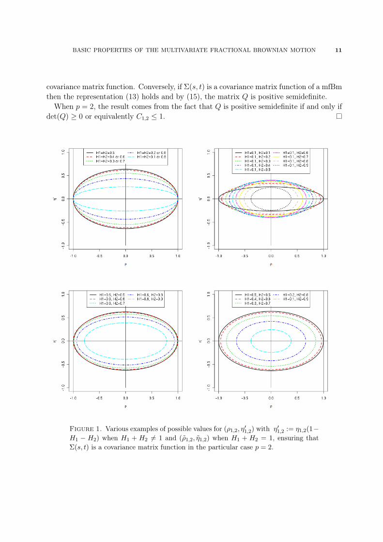
Figure 1. Various examples of possible values for (!1,2, "#1,2) with "#1,2 := "1,2(1"H1 " H2) when H1 + H2 #= 1 and (!1,2, "1,2) when H1 + H2 = 1, ensuring that!(s, t) is a covariance matrix function in the particular case p = 2.


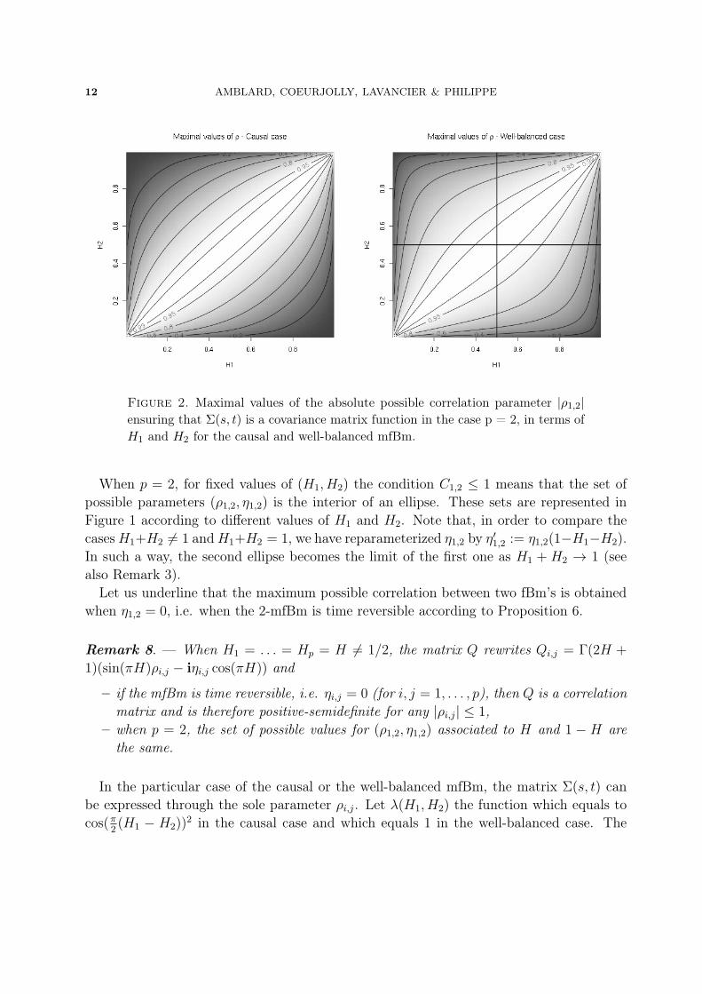
Figure 2. Maximal values of the absolute possible correlation parameter |!1,2|ensuring that !(s, t) is a covariance matrix function in the case p = 2, in terms ofH1 and H2 for the causal and well-balanced mfBm.

When p = 2, for fixed values of (H1, H2) the condition C1,2 * 1 means that the set ofpossible parameters (#1,2, $1,2) is the interior of an ellipse. These sets are represented inFigure 1 according to di"erent values of H1 and H2. Note that, in order to compare thecases H1+H2 #= 1 and H1+H2 = 1, we have reparameterized $1,2 by $#1,2 := $1,2(1"H1"H2).In such a way, the second ellipse becomes the limit of the first one as H1 + H2 % 1 (seealso Remark 3).

Let us underline that the maximum possible correlation between two fBm’s is obtainedwhen $1,2 = 0, i.e. when the 2-mfBm is time reversible according to Proposition 6.

Remark 8. — When H1 = . . . = Hp = H #= 1/2, the matrix Q rewrites Qi,j = "(2H +1)(sin(*H)#i,j " i$i,j cos(*H)) and

– if the mfBm is time reversible, i.e. $i,j = 0 (for i, j = 1, . . . , p), then Q is a correlationmatrix and is therefore positive-semidefinite for any |#i,j| * 1,

– when p = 2, the set of possible values for (#1,2, $1,2) associated to H and 1 " H arethe same.

In the particular case of the causal or the well-balanced mfBm, the matrix #(s, t) canbe expressed through the sole parameter #i,j. Let !(H1, H2) the function which equals tocos($2 (H1 " H2))2 in the causal case and which equals 1 in the well-balanced case. The


maximal possible correlation when p = 2 is given by

#21,2 ="(2H1 + 1)"(2H2 + 1)

"(H1 +H2 + 1)2sin(*H1) sin(*H2)

sin($2 (H1 +H2))2$ !(H1, H2).

Figure 2 represents |#1,2| with respect to (H1, H2).Figures 1 and 2 illustrate the main limitation of the mfBm model. Under self-similarity

condition (1), it is not possible to construct arbitrary correlated fractional Brownian mo-tions. For example, when H1 = 0.1 and H2 = 0.8, the correlation cannot exceed 0.514.

4. The mfBm as a limiting process.

A natural way to construct self-similar processes is through limits of stochastic processes.In dimension one, the result is due to Lamperti [18]. In [16], an extension to operatorself-similar processes is given. A similar result for the mfBm is deduced and stated below.In the following, a p-multivariate process (X(t))t!R is said proper if, for each t, the law ofX(t) is not contained in a proper subspace of Rp.

Theorem 10. — Let (X(t))t!R be a p-multivariate proper process, continuous in proba-bility. If there exist a p-multivariate process (Y (t))t!R and p real functions a1, ...., ap suchthat

(17) (a1(n)Y1(nt), . . . , ap(n)Yp(nt))n%&"""%fidi

X(t),

then the multivariate process (X(t)) is self-similar. Conversely, any multivariate self-similar process can be obtained as a such limit.

Proof. — The proof is similar to Theorem 5 in [16]. Fix k ! N and r > 0. For eachT ! Rk we denote X(T ) := (X(T1), . . . , X(Tk)). Let Dr,k be the set of all invertiblediagonal matrices ( such that, for all T ! Rk, X(rT ) = (X(T ).

Let us first show that Dr,k is not empty. According to (17), we have

diag(a1(n), . . . , ap(n))Y (nrT )n%&"""%

dX(rT ),

anddiag(a1(rn), . . . , ap(rn))Y (nrT )

n%&"""%d

X(T ).

Since (X(t)) is proper, diag(a1(n), . . . , ap(n)) and diag(a1(rn), . . . , ap(rn)) are invertiblefor n large enough. Then, Theorem 2.3 in [31] ensures that (n defined by

(n = diag(a1(n), . . . , ap(n))diag(a1(nr), . . . , ap(nr))"1

has a limit in Dr,k. Moreover if ( is a limit of (n then X(rT ) = (X(T ) and thus Dr,k #= +.


It is then straightforward to adapt Lemma 7.2-7.5 in [16] for the subgroup Dr,k, whichyields that for each r, ,kDr,k is not empty. Therefore, for any fixed r > 0, there ex-ists ( ! ,kDr,k such that (X(rt)) and ((X(T )) have the same finite dimensional dis-tributions. Theorem 1 in [16] ensures that there exists (H1, . . . , Hp) ! (0, 1)p such that( = diag(rH1 , . . . , rHp). The converse is trivial.

As an illustration of Theorem 10, the mfBm can be obtained as the weak limit of partialsums of sum of linear processes (also called superlinear processes, see [33]). Some examplesmay be found in [8] and [19]. In Proposition 11 below, we give a general convergence resultwhich allows to reach almost any mfBm from such partial sums. The unique restrictionconcerns the particular case when at least one of the Hurst parameters is equal to 1/2.

Let (,j(k))k!Z , j = 1, . . . , p be p independent i.i.d. sequences with zero mean and unitvariance. Let us consider the superlinear processes

(18) Zi(t) =p,

j=1

,

k!Z

-i,j(t" k),j(k), i = 1, . . . , p,

where -i,j(k) are real coe!cients with5

k!Z -2i,j(k) < '.

Moreover, we assume that -i,j(k) = -+i,j(k) + -"

i,j(k) where -+i,j(k) satisfies one of the

following conditions:

(i) -+i,j(k) =

!(+i,j + o(1)

"kd+i,j"1+ as |k| % ', with 0 < d+i,j <

12 and (+

i,j #= 0,

(ii) -+i,j(k) =

!(+i,j + o(1)

"kd+i,j"1+ as |k| % ', with "1

2 < d+i,j < 0,5

k!Z -+i,j(k) = 0 and

(+i,j #= 0,

(iii)5

k!Z))-+

i,j(k))) < ' and let (+

i,j :=5

k!Z -+i,j(k) #= 0, d+i,j := 0.

Similarly, -"i,j(k) is assumed to satisfy (i), (ii) or (iii) where k+, d+i,j and (+

i,j are replacedby k", d"i,j and ("

i,j.

Proposition 11. — Let di = max(d+i1, d"i1, · · · , d+ip, d"ip), for i = 1, . . . , p. Consider the

vector of partial sums, for + ! R,

Sn(+) =

6

7n"d1"(1/2)

[n% ],

t=1

Z1(t), · · · , n"dp"(1/2)

[n% ],

t=1

Zp(t)

8

9 .

Then the finite dimensional distributions of (Sn(+))%!R converge in law towards a p-mfBm(X(+))%!R.

– When di #= 0, (Xi(+))%!R is defined through the integral representation (16) whereM+

i,j = (+i,jd

"1i 1d+i,j=di

and M"i,j = ("

i,jd"1i 1d!i,j=di

.– When di = 0, Xi(+) =

5pj=1((

+i,j1d+i,j=0 + ("

i,j1d!i,j=0)Wj(+), where Wj is a standardBrownian motion.


Moreover, if for all j = 1, . . . , p, E(,j(0)2") < ' with ( > 1 - (1 + 2dmax)"1 wheredmax = maxi{di}, then Sn(.) converges towards the p-mfBm X(.) in the Skorohod spaceD([0, 1]).

Sketch of proof. — We focus on the convergence in law of Sn(+) to X(+), for a fixed + inR, the finite dimensional convergence is deduced in the same way. We set for simplicity+ = 1.

According to the Cramér-Wold device, for any vector (!1, . . . ,!p) ! Rp, we must showthat !#Sn(1) converges in law to !#X(1). We may rewrite !#Sn(1) as a sum of discretestochastic integrals (see [29] and [4]) :

!#Sn(1) =p,

i=1

!in"di"(1/2)

n,

t=1

Zi(t)

=p,

i=1

!i

p,

j=1

,

k!Z

n"di"(1/2)n,

t=1

(-+i,j(t" k) + -"

i,j(t" k)),j(k)

=p,

i=1

!i

p,

j=1

(

R(f+

i,j,n(x) + f"i,j,n(x))Wj,n(dx),(19)

where the stochastic measures Wj,n, j = 1, . . . , p are defined on finite intervals C by

Wj,n(C) = n"1/2,

k/n!C

,j(k),

and where f+i,j,n, f

"i,j,n are piecewise constant functions defined as follows: denoting .x/ the

smallest integer not less than x, we have for all x ! R,

f+i,j,n(x) = n"di

n,

t=1

-+i,j(t" .nx/),

respectively f"i,j,n(x) = n"di

5nt=1 -

"i,j(t" .xn/).

The following lemma states the convergence of a linear combination of discrete stochasticintegrals as in (19). A function is said n-simple if it takes a finite number a nonzero constantvalues on intervals (k/n, (k + 1)/n], k ! Z.

Lemma 12. — Let (f1,n, · · · , fp,n)n!N be a sequence of p n-simple functions in L2(R).If for any j = 1, . . . , p, there exists fj ! L2(R) such that

:R |fj,n(x) " fj(x)|2dx % 0,

then5p

j=1

:R fj,n(x)Wj,n(dx) converges in law to

5pj=1

:R fj(x)Wj(dx), where the Wj’s are

independent standard Gaussian random measures.

When p = 1, this lemma is proved in [28]. The case p = 2 is considered in [4] and theextension to p ( 3 is straightforward.


From Lemma 12 and (19), it remains to show that

limn%&

(

R

)))))f±i,j,n(x)"

(±i,j

di

!(1" x)di± " ("x)di±

"1d±i,j=di

)))))

2

dx = 0,

where we agree that d"1i ((1"x)di±"("x)di± ) = 1[0,1](x) when di = 0. Below, we only consider

the pointwise convergence of f±i,j,n(x), for x ! R, when d±i,j = di. The convergence in L2 is

then deduced from the dominated convergence theorem (see [28], [29], [4] for details). Italso follows easily that, when d±i,j < di,

:R |f

±i,j,n(x)|2dx % 0.

Under assumption (i), note that since di > 0, (1 " x)di± " ("x)di± = di: 1

0 (t " x)di"1± dt.

We have, for any x ! R,

f±i,j,n(x) = n"di

n,

t=1

-±i,j(t" .nx/)

= n"di

( n

0

-±i,j(.t/ " .nx/)dt

= n"di

( n

0

!(±i,j + o(1)

"(.t/ " .nx/)di"1

± dt

=

( 1

0

!(±i,j + o(1)

"&.nt/ " .nx/n

'di"1

±dt "% (±

i,j

( 1

0

(t" x)di"1± dt.

Under assumption (ii), di < 0. When x * 0, (1" x)di+ " ("x)di+ = di: 1

0 (t" x)di"1dt andthe convergence of f+

i,j,n(x) can be proved as above. When x ( 1, (1 " x)di+ " ("x)di+ =

0 = f+i,j,n(x). When 0 * x * 1, (1 " x)di+ " ("x)di+ = "di

: +&1 (t " x)di"1dt and, since5

k!Z -+i,j(k) = 0, we have

f+i,j,n(x) = n"di

n,

t='nx(

-+i,j(t" .nx/) = n"di

n"'nx(,

t=0

-+i,j(t) = "n"di

,

t>n"'nx(

-+i,j(t).

Therefore,

f+i,j,n(x) = "n"di

( +&

n"'nx(

!(+i,j + o(1)

"(.t/)di"1dt

= "( +&

1" "nx#n

!(+i,j + o(1)

"&.nt/n

'di"1

dt

"% "(+i,j

( +&

1"x

tdi"1dt = "(+i,j

( +&

1

(t" x)di"1dt

This proves f+i,j,n(x) % d"1

i (+i,j((1 " x)di+ " ("x)di+ ), for any x ! R, under assumption (ii).

The same scheme may be used to prove that f"i,j,n(x) % d"1

i ("i,j((1" x)di" " ("x)di" ) under


assumption (ii), noting that

(1" x)di" " ("x)di" =

;<<=

<<>

0 when x * 0,

"di: 0

"&(t" x)di"1dt when 0 * x * 1,

di: 1

0 (t" x)di"1" dt when x > 1.

Under assumption (iii),

f±i,j,n(x) =

n,

t=1

-±i,j(t" .nx/) =

n"'nx(,

t=1"'nx(

-±i,j(t).

Since5

t!Z -±i,j(t) < ', f±

i,j,n(x) % 0 for all x /! [0, 1]. When x ! [0, 1], we have f±i,j,n(x) %

(±i,j.Therefore, the first claim of the theorem is proved, i.e. the convergence in law of the finite

dimensional distribution of (Sn(+))%!R to (X(+))%!R. To extend this convergence to a func-tional convergence in D([0, 1]), it remains to show tightness of the sequence (Sn(+))%![0,1].This follows exactly from the same arguments as in the proof of Theorem 1.2 in [4].

5. Synthesis of the mfBm

5.1. Introduction. — The exact simulation of the fractional Brownian motion has beena question of great interest in the nineties. This may be done by generating a sample pathof a fractional Gaussian noise. An important step towards e!cient simulation was obtainedafter the work of Wood and Chan [32] about the simulation of arbitrary stationary Gaussiansequences with prescribed covariance function. The technique relies upon the embeddingof the covariance matrix into a circulant matrix, a square root of which is easily calculatedusing the discrete Fourier transform. This leads to a very e!cient algorithm, both in termsof computation time and storage needs. Wood and Chan method is an exact simulationmethod provided that the circulant matrix is semidefinite positive, a property that is notalways satisfied. However, for the fractional Gaussian noise, it can be proved that thecirculant matrix is definite positive for all H ! (0, 1), see [9, 13].

In [7], Wood and Chan extended their method and provided a more general algorithmadapted to multivariate stationary Gaussian processes. The main characteristic of thismethod is that if a certain condition for a familiy of Hermitian matrices holds then thealgorithm is exact in principle, i.e. the simulated data have the true covariance. We presenthereafter the main ideas, briefly describe the algorithm and propose some examples.

Remark 9. — Other approaches could have been undertaken (see [3] for a review in thecase p = 1). Approximate simulations can be done by discretizing the moving-average orspectral stochastic integrals (13) or (16). [6] also proposed an approximate method based on


the spectral density matrix of the increments for synthesizing multivariate Gaussian timeseries. Thanks to Proposition 5, this could also be envisaged for the mfBm.

5.2. Method and algorithm. — For two arbitrary matrices A = (Aj,k) and B, we useA0 B to denote the Kronecker product of A and B that is the block matrix (Aj,kB).

Let !X := !1X denotes the increments of size 1 (% = 1) of a mfBm. We have!X = (!X(t))t!R = ((!X1(t), . . . ,!Xp(t))#)t!R. The aim is to simulate a realizationof a multivariate fractional Gaussian noise discretized at times j = 1, . . . , n, that is a real-ization of (!X(1), . . . ,!X(n)). Then a realization of the discretized mfBm will be easilyobtained.

We denote by !X(n) the merged vector !X(n) = (!X(1)#, . . . ,!X(n)#)# and by G itscovariance matrix. G is the np$np Toeplitz block matrix G = (G(|i"j|))i,j=1,...,n where forh = 0, . . . , n"1, G(h) is the p$p matrix given by G(h) := (&j,k(h))j,k=1,...,p. The simulationproblem can be viewed as the generation of a random vector following a Nnp(0,G). Thismay be done by computing G1/2 but the complexity of such a procedure is O(p3n2) forblock Toeplitz matrices. To overcome this numerical cost, the idea is to embed G into theblock circulant matrix C = circ{C(j), j = 0, . . . ,m " 1}, where m is a power of 2 greaterthan 2(n" 1) and where each C(j) is the p$ p matrix defined by

(20) C(j) =

;=

>

G(j) if 0 * j < m/212

!G(j) +G(j)#

"if j = m/2

G(j "m) if m/2 < j * m" 1.

Such a definition ensures that C is a symmetric matrix with nested block circulant structureand that G = {C(j), j = 0, . . . , n " 1} is a submatrix of C. Therefore, the simulation ofa Nnp(0,G) may be achieved by taking the n “first” components of a vector Nmp(0, C),which is done by computing C1/2. The last problem is more simple since one may exploitthe circulant characteristic of C: there exist m Hermitian matrices B(j) of size p$ p suchthat the following decomposition holds

(21) C = (J 0 Ip) diag(B(j), j = 0, . . . ,m" 1) (J$ 0 Ip),

where Q is the m$m unitary matrix defined for j, k = 0,m" 1 by Jj,k = e"2i$jk/m. Thecomputation of C1/2 is much less expensive than the computation of G1/2 since, as in theone-dimensional case (p = 1), (21) will allow us to make use of the Fast Fourier Transform(FFT) which considerable reduces the complexity.

Now, the algorithm proposed by Wood and Chan may be described through the followingsteps. Let m be a power of 2 greater than 2(n" 1).Step 1. For 1 * u * v * p calculate for k = 0, . . . ,m" 1

Bu,v(k) =m"1,

j=0

Cu,v(j)e"2i$jk/m


where Cu,v(j) if the element (u, v) of the matrix C(j) defined by (20) and setBv,u(k) = Bu,v(k)$.

Step 2. For each j = 0, . . . ,m" 1 determine a unitary matrix R(j) and real numbers .u(j)(u = 1, . . . , p) such that B(j) = R(j) diag(.1(j), . . . , .p(j)) R(j)$.

Step 3. Assume that the eigenvalues .1(j), . . . , .p(j) are non-negative (see Remark 11) anddefine ?B(j) = R(j) diag(

2.1(j), . . . ,

2.p(j)) R(j)$.

Step 4. For j = 0, . . . ,m/2 generate independent vectors U(j), V (j) & Np(0, I) and define

Z(j) =1)2m

$% )

2U(j) for j = 0, m2U(j) + iV (j) for j = 1, . . . , m2 " 1,

let Z(m" j) = Z(j) for j = m2 + 1, . . . ,m" 1 and set W (j) := ?B(j)Z(j).

Step 5. For u = 1, . . . , p calculate for k = 0, . . . ,m" 1

!Xu(k) =m"1,

j=0

Wu(j)e"2i$jk/m

and return#!Xu(k), 1 * u * p, k = 0, . . . , n" 1

$.

Step 6. For u = 1, . . . , p take the cumulative sums !Xu to get the u " th component Xu

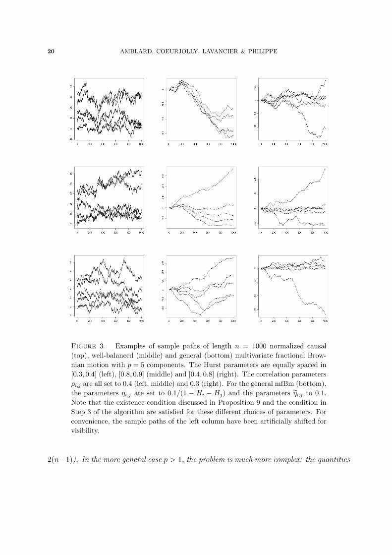
of a sample path of a mfBm.Figure 3 gives some examples of sample paths of mfBm’s simulated with this algorithm.

Remark 10. — Let us discuss the computation cost of the most expensive steps, that issteps 1, 2 and 5. Step 1 requires p(p+1)

2 applications of the FFT of signals of length m, Step2 needs m diagonalisations of p$ p Hermitian matrices and Step 5 requires p applicationsof the FFT of signals of length m. Therefore, the total cost, '(m, p) equals

'(m, p) = O&p(p+ 1)

2m logm

'+O(mp3) +O(pm logm).

Remark 11. — The crucial point of the previous algorithm lies in the non-negativity ofthe eigenvalues .1(j), . . . , .p(j) for any j = 0, . . . ,m"1. In the one-dimensional case (whenp = 1) Steps 2 and 3 disappear, and in Step 1, B11(k) corresponds to the k"th eigenvalueof the circulant matrix C11 with first line defined by C11(j) = &11(j) for 0 * j * m/2 and&(m" j) for j = m/2+1, . . . ,m" 1. For the fractional Gaussian noise, it has been provedby Craigmile [9] for H < 1/2, and by Dietrich and Newsam [13] for H > 1/2 that sucha matrix is semidefinite-positive for any m (and so for the first power of 2 greater than


Figure 3. Examples of sample paths of length n = 1000 normalized causal(top), well-balanced (middle) and general (bottom) multivariate fractional Brow-nian motion with p = 5 components. The Hurst parameters are equally spaced in[0.3, 0.4] (left), [0.8, 0.9] (middle) and [0.4, 0.8] (right). The correlation parameters!i,j are all set to 0.4 (left, middle) and 0.3 (right). For the general mfBm (bottom),the parameters "i,j are set to 0.1/(1 " Hi " Hj) and the parameters ?"i,j to 0.1.Note that the existence condition discussed in Proposition 9 and the condition inStep 3 of the algorithm are satisfied for these di!erent choices of parameters. Forconvenience, the sample paths of the left column have been artificially shifted forvisibility.

2(n"1)). In the more general case p > 1, the problem is much more complex: the quantities


Bu,v(k) are not necessarily real, and the establishment of a condition of positivity for thematrix Bu,v(k) does not seem obvious. When the condition in Step 3 does not hold, Woodand Chan suggest to either increase the value of m and restart Steps 1,2 or to truncatethe negative eigenvalues to zero which leads to an approximate procedure. These problemsare not addressed in this paper. Let us assert that for the simulation examples presentedin Figure 3, we have observed that this condition is satisfied for m equal to the first powerof2.

References

[1] Achard, S., Bassett, D. S., Meyer-Lindenberg, A. and Bullmore, E. (2008) Fractal connectivityof long-memory networks. Physical Review E, 77:036104.

[2] Arianos, S. and Carbone, A. (2009) Cross-correlation of long-range correlated series. Journalof Statistical Mechanics : Theory and Experiment, page P03037.

[3] Bardet, J.-M., Lang, G., Oppenheim, G., Philippe, A. and Taqqu, M. (2003) Generators oflong-range dependent processes : A survey. In: Doukhan, P., Oppenheim, G., Taqqu, M.S.(Eds.), Theory and Applications of Long-Range Dependence: Theory and Applications, pp. 557–578. Birkhäuser, Boston.

[4] Bru"aite, K. and Vai#iulis, M., (2005) Asymptotic independence of distant partial sums oflinear process. Lithuanian Mathematical Journal 45, 387–404.

[5] Coeurjolly, J.-F., Amblard, P.O., Achard, S., (2012) Wavelet analysis of the multivariatefractional Brownian motion, submitted arXiv:1007.2109.

[6] Chambers, J. (1995) The simulation of random vector time series with given spectrum. Math-ematical and Computer Modelling, 22, 1–6.

[7] Chan, G. and Wood, A. (1999) Simulation of stationary gaussian vector fields. Statistics andComputing, 9(4), 265–268.

[8] Chung, C.-F. (2002) Sample means, sample autocovariances, and linear regression of stationarymultivariate long memory processes. Econometric Theory 18, 51–78.

[9] Craigmile P. (2003) Simulating a class of stationary gaussian processes using the davies-hartealgortihm, with application to long memory processes. Journal of Time Series Analysis, 24,505–510.

[10] Davidson, J. and de Jong, R.M. (2000) The functional central limit theorem and weak con-vergence to stochastic integrals. Econometric Theory 16, 643–666.

[11] Davidson, J. and Hashimadze, N. (2008) Alternative frequency and time domain versions offractional Brownian motion. Econometric Theory 24, 256–293.

[12] Didier, G. and Pipiras, V. (2011) Integral representations of operator fractional Brownianmotion. Bernoulli 17(11) 1–33.

[13] Dietrich, C. R. and Newsam, G. N. (1997) Fast and exact simulation of stationary gaussianprocesses through circulant embedding of the covariance matrix. SIAM Journal on Scientific andStatistical Computing, 18, 1088 - 1107.

[14] Fleming B.J.W., Yu D., Harrison R.G. and Jubb D. (2001) Wavelet-based detection of co-herent structures and self-a$nity in financial data. The European Physical Journal B, 20(4),543-546.


[15] Gil-Alana L.A. (2003) A fractional multivariate long memory model for the US and theCanadian real output. Economics Letters, 81(3), 355-359.

[16] Hudson, W. and Mason, J. (1982) Operator-self-similar processes in a finite-dimensionalspace. Transactions of the American Mathematical Society 273, 281–297.

[17] Laha, R.G. and Rohatgi, V.K. (1981) Operator self-similar stochastic processes in Rd.Stochastic Processes and their Applications 12, 73–84.

[18] Lamperti J. (1962) Semi-Stable Stochastic Processes. Transactions of the American Mathe-matical Society, 104(1), pp. 62-78

[19] Lavancier, F., Philippe, A. and Surgailis, D. (2010) A two-sample test for comparison of longmemory parameters. Journal of Multivariate Analysis. 101 (9), pp 2118-2136.

[20] Lavancier, F., Philippe, A. and Surgailis, D. (2009) Covariance function of vector self-similarprocess. Statistics and Probability Letters. 79, 2415-2421.

[21] Maejima, M. and Mason, J. (1994) Operator-self-similar stable processes. Stochastic Processesand their Applications 54, 139–163.

[22] Mandelbrot, B. and Van Ness, J. (1968) Fractional Brownian motions, fractional noises andapplications. SIAM Review, 10(4), 422–437

[23] Marinucci, D. and Robinson, P.M. (2000) Weak convergence of multivariate fractional pro-cesses. Stochastic Processes and their Applications 86, 103–120.

[24] Robinson, P.M. (2008) Multiple local Whittle estimation in stationary systems. Annals ofStatistics. 36, 2508–2530.

[25] Samorodnitsky, G. and Taqqu, M.S. (1994) Stable Non-Gaussian Random Processes.Chapman and Hall, New York.

[26] Sato, K. (1991) Self-similar processes with independent increments. Probability Theory andRelated Fields 89, 285–300.

[27] Stoev, S. and Taqqu, M.S. (2006) How rich is the class of multifractional Brownian motions?Stochastic Processes and their Applications. 11, 200–221.

[28] Surgailis, D. (1982). Zones of attraction of self-similar multiple integrals. Lithuanian Mathe-matical Journal. 22, 185 201.

[29] Surgailis, D. (2003) Non CLTs: U-statistics, multinomial formula and approximations ofmultiple Itô-Wiener integrals. In: Doukhan, P., Oppenheim, G., Taqqu, M.S. (Eds.), Theory andApplications of Long-Range Dependence: Theory and Applications, pp. 129–142. Birkhäuser,Boston.

[30] Taqqu, M. (2003) Fractional Brownian motion and long-range dependence In: Doukhan,P., Oppenheim, G., Taqqu, M.S. (Eds.), Theory and Applications of Long-Range Dependence:Theory and Applications, pp. 5–38. Birkhäuser, Boston.

[31] Weissman, I. (1976) On convergence of types and processes in Euclidean space. ProbabilityTheory and Related Fields 37(1), 35–41.

[32] Wood, A. and Chan, G. (1994) Simulation of stationary gaussian processes in [0, 1]d. Journalof computational and graphical statistics, 3, 409–432.

[33] Zhao, O. and Woodroofe, M. (2008) On martingale approximations. Annals of Applied Prob-ability. 18, 1831-1847.


Amblard, Dept. Math & Stat., The University of Melbourne, Parkville, VIC 3010, Australia,and, GIPSAlab/CNRS UMR 5216/ BP 46, 38402 Saint Martin d’Hères cedex, FranceE-mail : [email protected] : http://www.gipsa-lab.grenoble-inp.fr/~bidou.amblard/

Coeurjolly, Laboratoire Jean Kuntzmann, UMR 5224, BSHM, 1251 Av. Centrale BP 47,, 38040Grenoble Cedex 9 FRANCE, and, GIPSAlab/CNRS UMR 5216/ BP 46, 38402 Saint Martind’Hères cedex, France • E-mail : [email protected] : http://www-ljk.imag.fr/membres/Jean-Francois.Coeurjolly/

Lavancier, Université de Nantes, Laboratoire de mathématiques Jean Leray, 2, rue de la Houssinière44322 Nantes, France • E-mail : [email protected] : http://www.math.sciences.univ-nantes.fr/~lavancie

Philippe, Université de Nantes, Laboratoire de mathématiques Jean Leray, 2, rue de la Houssinière44322 Nantes, France • E-mail : [email protected] : http://www.math.sciences.univ-nantes.fr/~philippe

Documents

BASIC PROPERTIES OF THE MULTIVARIATE FRACTIONAL BROWNIAN ... · Research supported in part by ANR STARAC grant and a fellowship from Région Rhône-Alpes ... A multivariate extension