Embed Size (px)
Citation preview

Basic Complex AnalysisA Comprehensive Course in Analysis, Part 2A
Barry Simon
Licensed to AMS.
License or copyright restrictions may apply to redistribution; see http://www.ams.org/publications/ebooks/terms

Basic Complex Analysis A Comprehensive Course in Analysis, Part 2A
Licensed to AMS.
License or copyright restrictions may apply to redistribution; see http://www.ams.org/publications/ebooks/terms

Licensed to AMS.
License or copyright restrictions may apply to redistribution; see http://www.ams.org/publications/ebooks/terms
Basic Complex Analysis A Comprehensive Course in Analysis, Part 2A
Barry Simon
Providence, Rhode Island
http://dx.doi.org/10.1090/simon/002.1
Licensed to AMS.
License or copyright restrictions may apply to redistribution; see http://www.ams.org/publications/ebooks/terms

2010 Mathematics Subject Classification. Primary 30-01, 33-01, 40-01;Secondary 34-01, 41-01, 44-01.
For additional information and updates on this book, visitwww.ams.org/bookpages/simon
Library of Congress Cataloging-in-Publication Data
Simon, Barry, 1946–Basic complex analysis / Barry Simon.
pages cm. — (A comprehensive course in analysis ; part 2A)Includes bibliographical references and indexes.ISBN 978-1-4704-1100-8 (alk. paper)1. Mathematical analysis—Textbooks. I. Title.
QA300.S527 2015515—dc23
2015009337
Copying and reprinting. Individual readers of this publication, and nonprofit librariesacting for them, are permitted to make fair use of the material, such as to copy select pages foruse in teaching or research. Permission is granted to quote brief passages from this publication inreviews, provided the customary acknowledgment of the source is given.
Republication, systematic copying, or multiple reproduction of any material in this publicationis permitted only under license from the American Mathematical Society. Permissions to reuseportions of AMS publication content are handled by Copyright Clearance Center’s RightsLink�service. For more information, please visit: http://www.ams.org/rightslink.
Send requests for translation rights and licensed reprints to [email protected] from these provisions is material for which the author holds copyright. In such cases,
requests for permission to reuse or reprint material should be addressed directly to the author(s).Copyright ownership is indicated on the copyright page, or on the lower right-hand corner of thefirst page of each article within proceedings volumes.
c© 2015 by the American Mathematical Society. All rights reserved.The American Mathematical Society retains all rightsexcept those granted to the United States Government.
Printed in the United States of America.
©∞ The paper used in this book is acid-free and falls within the guidelinesestablished to ensure permanence and durability.
Visit the AMS home page at http://www.ams.org/
10 9 8 7 6 5 4 3 2 1 20 19 18 17 16 15
Licensed to AMS.
License or copyright restrictions may apply to redistribution; see http://www.ams.org/publications/ebooks/terms

To the memory of Cherie Galvez
extraordinary secretary, talented helper, caring person
and to the memory of my mentors,
Ed Nelson (1932-2014) and Arthur Wightman (1922-2013)
who not only taught me Mathematics
but taught me how to be a mathematician
Licensed to AMS.
License or copyright restrictions may apply to redistribution; see http://www.ams.org/publications/ebooks/terms

Licensed to AMS.
License or copyright restrictions may apply to redistribution; see http://www.ams.org/publications/ebooks/terms

Contents
Preface to the Series xi
Preface to Part 2 xvii
Chapter 1. Preliminaries 1
§1.1. Notation and Terminology 1
§1.2. Complex Numbers 3
§1.3. Some Algebra, Mainly Linear 5
§1.4. Calculus on R and Rn 8
§1.5. Differentiable Manifolds 12
§1.6. Riemann Metrics 18
§1.7. Homotopy and Covering Spaces 21
§1.8. Homology 24
§1.9. Some Results from Real Analysis 26
Chapter 2. The Cauchy Integral Theorem: Basics 29
§2.1. Holomorphic Functions 30
§2.2. Contour Integrals 40
§2.3. Analytic Functions 49
§2.4. The Goursat Argument 66
§2.5. The CIT for Star-Shaped Regions 69
§2.6. Holomorphically Simply Connected Regions, Logs, andFractional Powers 71
§2.7. The Cauchy Integral Formula for Disks and Annuli 76
vii
Licensed to AMS.
License or copyright restrictions may apply to redistribution; see http://www.ams.org/publications/ebooks/terms

viii Contents
Chapter 3. Consequences of the Cauchy Integral Formula 79
§3.1. Analyticity and Cauchy Estimates 80
§3.2. An Improved Cauchy Estimate 93
§3.3. The Argument Principle and Winding Numbers 95
§3.4. Local Behavior at Noncritical Points 104
§3.5. Local Behavior at Critical Points 108
§3.6. The Open Mapping and Maximum Principle 114
§3.7. Laurent Series 120
§3.8. The Classification of Isolated Singularities;Casorati–Weierstrass Theorem 124
§3.9. Meromorphic Functions 128
§3.10. Periodic Analytic Functions 132
Chapter 4. Chains and the Ultimate Cauchy Integral Theorem 137
§4.1. Homologous Chains 139
§4.2. Dixon’s Proof of the Ultimate CIT 142
§4.3. The Ultimate Argument Principle 143
§4.4. Mesh-Defined Chains 145
§4.5. Simply Connected and Multiply Connected Regions 150
§4.6. The Ultra Cauchy Integral Theorem and Formula 151
§4.7. Runge’s Theorems 153
§4.8. The Jordan Curve Theorem for Smooth Jordan Curves 161
Chapter 5. More Consequences of the CIT 167
§5.1. The Phragmen–Lindelof Method 168
§5.2. The Three-Line Theorem and the Riesz–ThorinTheorem 174
§5.3. Poisson Representations 177
§5.4. Harmonic Functions 183
§5.5. The Reflection Principle 189
§5.6. Reflection in Analytic Arcs; Continuity at AnalyticCorners 196
§5.7. Calculation of Definite Integrals 201
Chapter 6. Spaces of Analytic Functions 227
§6.1. Analytic Functions as a Frechet Space 228
§6.2. Montel’s and Vitali’s Theorems 234
Licensed to AMS.
License or copyright restrictions may apply to redistribution; see http://www.ams.org/publications/ebooks/terms

Contents ix
§6.3. Restatement of Runge’s Theorems 244
§6.4. Hurwitz’s Theorem 245
§6.5. Bonus Section: Normal Convergence of MeromorphicFunctions and Marty’s Theorem 247
Chapter 7. Fractional Linear Transformations 255
§7.1. The Concept of a Riemann Surface 256
§7.2. The Riemann Sphere as a Complex Projective Space 267
§7.3. PSL(2,C) 273
§7.4. Self-Maps of the Disk 289
§7.5. Bonus Section: Introduction to Continued Fractionsand the Schur Algorithm 295
Chapter 8. Conformal Maps 309
§8.1. The Riemann Mapping Theorem 310
§8.2. Boundary Behavior of Riemann Maps 319
§8.3. First Construction of the Elliptic Modular Function 325
§8.4. Some Explicit Conformal Maps 336
§8.5. Bonus Section: Covering Map for General Regions 353
§8.6. Doubly Connected Regions 357
§8.7. Bonus Section: The Uniformization Theorem 362
§8.8. Ahlfors’ Function, Analytic Capacity and the PainleveProblem 371
Chapter 9. Zeros of Analytic Functions and Product Formulae 381
§9.1. Infinite Products 383
§9.2. A Warmup: The Euler Product Formula 387
§9.3. The Mittag-Leffler Theorem 399
§9.4. The Weierstrass Product Theorem 401
§9.5. General Regions 406
§9.6. The Gamma Function: Basics 410
§9.7. The Euler–Maclaurin Series and Stirling’sApproximation 430
§9.8. Jensen’s Formula 448
§9.9. Blaschke Products 451
§9.10. Entire Functions of Finite Order and the HadamardProduct Formula 459
Licensed to AMS.
License or copyright restrictions may apply to redistribution; see http://www.ams.org/publications/ebooks/terms

x Contents
Chapter 10. Elliptic Functions 475
§10.1. A Warmup: Meromorphic Functions on C 480
§10.2. Lattices and SL(2,Z) 481
§10.3. Liouville’s Theorems, Abel’s Theorem, and Jacobi’sConstruction 491
§10.4. Weierstrass Elliptic Functions 501
§10.5. Bonus Section: Jacobi Elliptic Functions 522
§10.6. The Elliptic Modular Function 542
§10.7. The Equivalence Problem for Complex Tori 552
Chapter 11. Selected Additional Topics 555
§11.1. The Paley–Wiener Strategy 557
§11.2. Global Analytic Functions 564
§11.3. Picard’s Theorem via the Elliptic Modular Function 570
§11.4. Bonus Section: Zalcman’s Lemma and Picard’sTheorem 575
§11.5. Two Results in Several Complex Variables:Hartogs’ Theorem and a Theorem of Poincare 580
§11.6. Bonus Section: A First Glance atCompact Riemann Surfaces 586
Bibliography 591
Symbol Index 623
Subject Index 625
Author Index 633
Index of Capsule Biographies 641
Licensed to AMS.
License or copyright restrictions may apply to redistribution; see http://www.ams.org/publications/ebooks/terms

Preface to the Series
Young men should prove theorems, old men should write books.
—Freeman Dyson, quoting G. H. Hardy1
Reed–Simon2 starts with “Mathematics has its roots in numerology, ge-ometry, and physics.” This puts into context the division of mathematicsinto algebra, geometry/topology, and analysis. There are, of course, otherareas of mathematics, and a division between parts of mathematics can beartificial. But almost universally, we require our graduate students to takecourses in these three areas.
This five-volume series began and, to some extent, remains a set of textsfor a basic graduate analysis course. In part it reflects Caltech’s three-terms-per-year schedule and the actual courses I’ve taught in the past. Much of thecontents of Parts 1 and 2 (Part 2 is in two volumes, Part 2A and Part 2B) arecommon to virtually all such courses: point set topology, measure spaces,Hilbert and Banach spaces, distribution theory, and the Fourier transform,complex analysis including the Riemann mapping and Hadamard producttheorems. Parts 3 and 4 are made up of material that you’ll find in some,but not all, courses—on the one hand, Part 3 on maximal functions andHp-spaces; on the other hand, Part 4 on the spectral theorem for boundedself-adjoint operators on a Hilbert space and det and trace, again for Hilbertspace operators. Parts 3 and 4 reflect the two halves of the third term ofCaltech’s course.
1Interview with D. J. Albers, The College Mathematics Journal, 25, no. 1, January 1994.2M. Reed and B. Simon, Methods of Modern Mathematical Physics, I: Functional Analysis,
Academic Press, New York, 1972.
xi
Licensed to AMS.
License or copyright restrictions may apply to redistribution; see http://www.ams.org/publications/ebooks/terms

xii Preface to the Series
While there is, of course, overlap between these books and other texts,there are some places where we differ, at least from many:
(a) By having a unified approach to both real and complex analysis, we areable to use notions like contour integrals as Stietljes integrals that crossthe barrier.
(b) We include some topics that are not standard, although I am sur-prised they are not. For example, while discussing maximal functions,I present Garcia’s proof of the maximal (and so, Birkhoff) ergodic the-orem.
(c) These books are written to be keepers—the idea is that, for many stu-dents, this may be the last analysis course they take, so I’ve tried towrite in a way that these books will be useful as a reference. For thisreason, I’ve included “bonus” chapters and sections—material that I donot expect to be included in the course. This has several advantages.First, in a slightly longer course, the instructor has an option of extratopics to include. Second, there is some flexibility—for an instructorwho can’t imagine a complex analysis course without a proof of theprime number theorem, it is possible to replace all or part of the (non-bonus) chapter on elliptic functions with the last four sections of thebonus chapter on analytic number theory. Third, it is certainly possibleto take all the material in, say, Part 2, to turn it into a two-term course.Most importantly, the bonus material is there for the reader to peruselong after the formal course is over.
(d) I have long collected “best” proofs and over the years learned a num-ber of ones that are not the standard textbook proofs. In this re-gard, modern technology has been a boon. Thanks to Google booksand the Caltech library, I’ve been able to discover some proofs thatI hadn’t learned before. Examples of things that I’m especially fondof are Bernstein polynomials to get the classical Weierstrass approxi-mation theorem, von Neumann’s proof of the Lebesgue decompositionand Radon–Nikodym theorems, the Hermite expansion treatment ofFourier transform, Landau’s proof of the Hadamard factorization theo-rem, Wielandt’s theorem on the functional equation for Γ(z), and New-man’s proof of the prime number theorem. Each of these appears in atleast some monographs, but they are not nearly as widespread as theydeserve to be.
(e) I’ve tried to distinguish between central results and interesting asidesand to indicate when an interesting aside is going to come up againlater. In particular, all chapters, except those on preliminaries, havea listing of “Big Notions and Theorems” at their start. I wish thatthis attempt to differentiate between the essential and the less essential
Licensed to AMS.
License or copyright restrictions may apply to redistribution; see http://www.ams.org/publications/ebooks/terms
Preface to the Series xiii
didn’t make this book different, but alas, too many texts are monotonelistings of theorems and proofs.
(f) I’ve included copious “Notes and Historical Remarks” at the end ofeach section. These notes illuminate and extend, and they (and theProblems) allow us to cover more material than would otherwise bepossible. The history is there to enliven the discussion and to emphasizeto students that mathematicians are real people and that “may you livein interesting times” is truly a curse. Any discussion of the history ofreal analysis is depressing because of the number of lives ended bythe Nazis. Any discussion of nineteenth-century mathematics makesone appreciate medical progress, contemplating Abel, Riemann, andStieltjes. I feel knowing that Picard was Hermite’s son-in-law spices upthe study of his theorem.
On the subject of history, there are three cautions. First, I am not aprofessional historian and almost none of the history discussed here is basedon original sources. I have relied at times—horrors!—on information on theInternet. I have tried for accuracy but I’m sure there are errors, some thatwould make a real historian wince.
A second caution concerns looking at the history assuming the mathe-matics we now know. Especially when concepts are new, they may be poorlyunderstood or viewed from a perspective quite different from the one here.Looking at the wonderful history of nineteenth-century complex analysis byBottazzini–Grey3 will illustrate this more clearly than these brief notes can.
The third caution concerns naming theorems. Here, the reader needsto bear in mind Arnol’d’s principle:4 If a notion bears a personal name,then that name is not the name of the discoverer (and the related Berryprinciple: The Arnol’d principle is applicable to itself ). To see the applica-bility of Berry’s principle, I note that in the wider world, Arnol’d’s principleis called “Stigler’s law of eponymy.” Stigler5 named this in 1980, pointingout it was really discovered by Merton. In 1972, Kennedy6 named Boyer’slaw Mathematical formulas and theorems are usually not named after theiroriginal discoverers after Boyer’s book.7 Already in 1956, Newman8 quotedthe early twentieth-century philosopher and logician A. N. Whitehead assaying: “Everything of importance has been said before by somebody who
3U. Bottazzini and J. Gray, Hidden Harmony—Geometric Fantasies. The Rise of ComplexFunction Theory, Springer, New York, 2013.
4V. I. Arnol’d, On teaching mathematics, available online at http://pauli.uni-muenster.
de/~munsteg/arnold.html.5S. M. Stigler, Stigler’s law of eponymy, Trans. New York Acad. Sci. 39 (1980), 147–158.6H. C. Kennedy, Classroom notes: Who discovered Boyer’s law?, Amer. Math. Monthly 79
(1972), 66–67.7C. B. Boyer, A History of Mathematics, Wiley, New York, 1968.8J. R. Newman, The World of Mathematics, Simon & Schuster, New York, 1956.
Licensed to AMS.
License or copyright restrictions may apply to redistribution; see http://www.ams.org/publications/ebooks/terms
xiv Preface to the Series
did not discover it.” The main reason to give a name to a theorem is to havea convenient way to refer to that theorem. I usually try to follow commonusage (even when I know Arnol’d’s principle applies).
I have resisted the temptation of some text writers to rename thingsto set the record straight. For example, there is a small group who haveattempted to replace “WKB approximation” by “Liouville–Green approxi-mation”, with valid historical justification (see the Notes to Section 15.5 ofPart 2B). But if I gave a talk and said I was about to use the Liouville–Greenapproximation, I’d get blank stares from many who would instantly knowwhat I meant by the WKB approximation. And, of course, those who try tochange the name also know what WKB is! Names are mainly for shorthand,not history.
These books have a wide variety of problems, in line with a multiplicityof uses. The serious reader should at least skim them since there is ofteninteresting supplementary material covered there.
Similarly, these books have a much larger bibliography than is standard,partly because of the historical references (many of which are available on-line and a pleasure to read) and partly because the Notes introduce lots ofperipheral topics and places for further reading. But the reader shouldn’tconsider for a moment that these are intended to be comprehensive—thatwould be impossible in a subject as broad as that considered in these vol-umes.
These books differ from many modern texts by focusing a little more onspecial functions than is standard. In much of the nineteenth century, thetheory of special functions was considered a central pillar of analysis. Theyare now out of favor—too much so—although one can see some signs of thependulum swinging back. They are still mainly peripheral but appear oftenin Part 2 and a few times in Parts 1, 3, and 4.
These books are intended for a second course in analysis, but in mostplaces, it is really previous exposure being helpful rather than required.Beyond the basic calculus, the one topic that the reader is expected to haveseen is metric space theory and the construction of the reals as completionof the rationals (or by some other means, such as Dedekind cuts).
Initially, I picked “A Course in Analysis” as the title for this series asan homage to Goursat’s Cours d’Analyse,9 a classic text (also translatedinto English) of the early twentieth century (a literal translation would be
9E. Goursat, A Course in Mathematical Analysis: Vol. 1: Derivatives and Differentials,Definite Integrals, Expansion in Series, Applications to Geometry. Vol. 2, Part 1: Functions of aComplex Variable. Vol. 2, Part 2: Differential Equations. Vol. 3, Part 1: Variation of Solutions.Partial Differential Equations of the Second Order. Vol. 3, Part 2: Integral Equations. Calculusof Variations, Dover Publications, New York, 1959 and 1964; French original, 1905.
Licensed to AMS.
License or copyright restrictions may apply to redistribution; see http://www.ams.org/publications/ebooks/terms

Preface to the Series xv
“of Analysis” but “in” sounds better). As I studied the history, I learned
that this was a standard French title, especially associated with Ecole Poly-technique. There are nineteenth-century versions by Cauchy and Jordanand twentieth-century versions by de la Vallee Poussin and Choquet. Sothis is a well-used title. The publisher suggested adding “Comprehensive”,which seems appropriate.
It is a pleasure to thank many people who helped improve these texts.About 80% was TEXed by my superb secretary of almost 25 years, CherieGalvez. Cherie was an extraordinary person—the secret weapon to myproductivity. Not only was she technically strong and able to keep my tasksorganized but also her people skills made coping with bureaucracy of allkinds easier. She managed to wind up a confidant and counselor for manyof Caltech’s mathematics students. Unfortunately, in May 2012, she wasdiagnosed with lung cancer, which she and chemotherapy valiantly fought.In July 2013, she passed away. I am dedicating these books to her memory.
During the second half of the preparation of this series of books, wealso lost Arthur Wightman and Ed Nelson. Arthur was my advisor andwas responsible for the topic of my first major paper—perturbation theoryfor the anharmonic oscillator. Ed had an enormous influence on me, bothvia the techniques I use and in how I approach being a mathematician. Inparticular, he taught me all about closed quadratic forms, motivating themethodology of my thesis. I am also dedicating these works to their memory.
After Cherie entered hospice, Sergei Gel’fand, the AMS publisher, helpedme find Alice Peters to complete the TEXing of the manuscript. Her experi-ence in mathematical publishing (she is the “A” of A K Peters Publishing)meant she did much more, for which I am grateful.
This set of books has about 150 figures which I think considerably addto their usefulness. About half were produced by Mamikon Mnatsakanian,a talented astrophysicist and wizard with Adobe Illustrator. The otherhalf, mainly function plots, were produced by my former Ph.D. student andteacher extraordinaire Mihai Stoiciu (used with permission) using Mathe-matica. There are a few additional figures from Wikipedia (mainly underWikiCommons license) and a hyperbolic tiling of Douglas Dunham, usedwith permission. I appreciate the help I got with these figures.
Over the five-year period that I wrote this book and, in particular, dur-ing its beta-testing as a text in over a half-dozen institutions, I receivedfeedback and corrections from many people. In particular, I should like tothank (with apologies to those who were inadvertently left off): Tom Al-berts, Michael Barany, Jacob Christiansen, Percy Deift, Tal Einav, GermanEnciso, Alexander Eremenko, Rupert Frank, Fritz Gesztesy, Jeremy Gray,
Licensed to AMS.
License or copyright restrictions may apply to redistribution; see http://www.ams.org/publications/ebooks/terms

xvi Preface to the Series
Leonard Gross, Chris Heil, Mourad Ismail, Svetlana Jitomirskaya, Bill John-son, Rowan Killip, John Klauder, Seung Yeop Lee, Milivoje Lukic, AndreMartinez-Finkelshtein, Chris Marx, Alex Poltoratski, Eric Rains, LorenzoSadun, Ed Saff, Misha Sodin, Dan Stroock, Benji Weiss, Valentin Zagreb-nov, and Maxim Zinchenko.
Much of these books was written at the tables of the Hebrew UniversityMathematics Library. I’d like to thank Yoram Last for his invitation andNaavah Levin for the hospitality of the library and for her invaluable help.
This series has a Facebook page. I welcome feedback, questions, andcomments. The page is at www.facebook.com/simon.analysis .
Even if these books have later editions, I will try to keep theorem andequation numbers constant in case readers use them in their papers.
Finally, analysis is a wonderful and beautiful subject. I hope the readerhas as much fun using these books as I had writing them.
Licensed to AMS.
License or copyright restrictions may apply to redistribution; see http://www.ams.org/publications/ebooks/terms

Preface to Part 2
Part 2 of this five-volume series is devoted to complex analysis. We’ve splitPart 2 into two pieces (Part 2A and Part 2B), partly because of the totallength of the current material, but also because of the fact that we’ve left outseveral topics and so Part 2B has some room for expansion. To indicate theview that these two volumes are two halves of one part, chapter numbersare cumulative. Chapters 1–11 are in Part 2A, and Part 2B starts withChapter 12.
The flavor of Part 2 is quite different from Part 1—abstract spaces areless central (although hardly absent)—the content is more classical and moregeometrical. The classical flavor is understandable. Most of the material inthis part dates from 1820–1895, while Parts 1, 3, and 4 largely date from1885–1940.
While real analysis has important figures, especially F. Riesz, it is hardto single out a small number of “fathers.” On the other hand, it is clearthat the founding fathers of complex analysis are Cauchy, Weierstrass, andRiemann. It is useful to associate each of these three with separate threadswhich weave together to the amazing tapestry of this volume. While useful,it is a bit of an exaggeration in that one can identify some of the otherthreads in the work of each of them. That said, they clearly did havedistinct focuses, and it is useful to separate the three points of view.
To Cauchy, the central aspect is the differential and integral calculus ofcomplex-valued functions of a complex variable. Here the fundamentals arethe Cauchy integral theorem and Cauchy integral formula. These are thebasics behind Chapters 2–5.
xvii
Licensed to AMS.
License or copyright restrictions may apply to redistribution; see http://www.ams.org/publications/ebooks/terms

xviii Preface to Part 2
For Weierstrass, sums and products and especially power series are thecentral object. These appear first peeking through in the Cauchy chapters(especially Section 2.3) and dominate in Chapters 6, 9, 10, and parts ofChapter 11, Chapter 13, and Chapter 14.
For Riemann, it is the view as conformal maps and associated geometry.The central chapters for this are Chapters 7, 8, and 12, but also parts ofChapters 10 and 11.
In fact, these three strands recur all over and are interrelated, but it isuseful to bear in mind the three points of view.
I’ve made the decision to restrict some results to C1 or piecewise C1
curves—for example, we only prove the Jordan curve theorem for that case.
We don’t discuss, in this part, boundary values of analytic functions inthe unit disk, especially the theory of the Hardy spaces, Hp(D). This is atopic in Part 3. Potential theory has important links to complex analysis,but we’ve also put it in Part 3 because of the close connection to harmonicfunctions.
Unlike real analysis, where some basic courses might leave out point settopology or distribution theory, there has been for over 100 years an ac-knowledged common core of any complex analysis text: the Cauchy integraltheorem and its consequences (Chapters 2 and 3), some discussion of har-monic functions on R2 and of the calculation of indefinite integrals (Chap-ter 5), some discussion of fractional linear transformations and of conformalmaps (Chapters 7 and 8). It is also common to discuss at least Weier-strass product formulas (Chapter 9) and Montel’s and/or Vitali’s theorems(Chapter 6).
I also feel strongly that global analytic functions belong in a basic course.There are several topics that will be in one or another course, notably theHadamard product formula (Chapter 9), elliptic functions (Chapter 10),analytic number theory (Chapter 13), and some combination of hypergeo-metric functions (Chapter 14) and asymptotics (Chapter 15). Nevanlinnatheory (Chapter 17) and univalents functions (Chapter 16) are almost al-ways in advanced courses. The break between Parts 2A and 2B is basedmainly on what material is covered in Caltech’s course, but the material isan integrated whole. I think it unfortunate that asymptotics doesn’t seemto have made the cut in courses for pure mathematicians (although the ma-terial in Chapters 14 and 15 will be in complex variable courses for appliedmathematicians).
Licensed to AMS.
License or copyright restrictions may apply to redistribution; see http://www.ams.org/publications/ebooks/terms

Chapter 1
Preliminaries
You know also that the beginning is the most important part of any work.
—Plato’s Republic [436]
This chapter sets notation and reviews various subjects that, it is hoped,the reader has seen before. For some, like calculus, the basic material isreally a prerequisite. Others, like covering spaces, are only used in a fewplaces, and enough background is given to perhaps tide over the studentwith less preparation. Essentially, Sections 1.1–1.4 are used often and therest sporadically.
1.1. Notation and Terminology
A foolish consistency is the hobgoblin of little minds . . . Is it so bad, then,to be misunderstood? Pythagoras was misunderstood, and Socrates, andJesus, and Luther, and Copernicus, and Galileo, and Newton, and everypure and wise spirit that ever took flesh. To be great is to be misunder-stood.
—Ralph Waldo Emerson [164]
For a real number a, we will use the terms positive and strictly positivefor a ≥ 0 and a > 0, respectively. It is not so much that we find nonnegativebad, but the phrase “monotone nondecreasing” for x > y ⇒ f(x) ≥ f(y) isdownright confusing so we use “monotone increasing” and “strictly mono-tone increasing” and then, for consistency, “positive” and “strictly positive.”Similarly for matrices, we use “positive definite” and “strictly positive defi-nite” where others might use “positive semi-definite” and “positive definite.”
1
http://dx.doi.org/10.1090/simon/002.1/01
Licensed to AMS.
License or copyright restrictions may apply to redistribution; see http://www.ams.org/publications/ebooks/terms

2 1. Preliminaries
Basic Rings and Fields.
R = real numbers Q = rationals Z = integers
C = complex numbers = {x+ iy | x, y ∈ R}
with their sums and products. For z = x + iy ∈ C, we use Re z = x,Im z = y. |z| = (x2 + y2)1/2.
Products. Xn = n-tuples of points in X with induced vector space and/oradditive structure; in particular, Rn, Qn, Zn, Cn.
Subsets of C (and one superset).
� C = C ∪ {∞} as a one-point compactification; in Section 7.2, we’ll puta complex structure near ∞.
� C+ = upper half-plane = {z | Im z > 0};H+ = right half-plane = {z | Re z > 0}
� Z+ = {n ∈ Z | n > 0} = {1, 2, 3, . . . };N = {0} ∪ Z+ = {0, 1, 2, . . . }
� D = {z ∈ C | |z| < 1}; ∂D = {z ∈ C | |z| = 1}� Dδ(z0) = {z ∈ C | |z − z0| < δ} for z0 ∈ C, δ > 0
� C× = C \ {0}; D× = D \ {0}; R× = R \ {0}(in general, Y × = invertible elements of Y )
� Ar,R = annulus = {z | r < |z| < R} for 0 ≤ r < R ≤ ∞� Sα,β = sector = {r(cos θ + i sin θ) | r > 0; α < θ < β} for α < β and|β − α| ≤ 2π; for example, S−π,π = C \ (−∞, 0]
Miscellaneous Terms.
� K a compact Hausdorff space, C(K) = continuous complex-valued func-tions on K
� For x ∈ R, [x] = greatest integer less than x, that is, [x] ∈ Z, [x] ≤ x <[x] + 1
� {x} = x− [x] = fractional parts of x
� �(A) = number of elements in a set A
� Ran f = range of a function f
� log(z) = natural logarithm, that is, logarithm to base e; if z is complex,put the cut along (−∞, 0], i.e., log(z) = log(|z|) + i arg(z) with −π <arg(z) ≤ π
� Region = open, connected subset of C
Licensed to AMS.
License or copyright restrictions may apply to redistribution; see http://www.ams.org/publications/ebooks/terms

1.2. Complex Numbers 3
� For sets A,B subsets of X, A∪B = union, A∩B = intersection, Ac =complement of A in X, A \B = A ∩Bc, AB = (A \B) ∪ (B \A)
� For matrices, M12 means row one, column two
� f � K = restriction of a function to K, a subset of the domain of f
Integer Notation (see Section 1.3 for modular arithmetic). This is mainlyrelevant in Chapter 13 of Part 2B. All letters in this subsection are in Z
� d | n means d is a divisor of n, that is, n = dk for k ∈ Z
� a ≡ b (mod m)⇔ m | a− b
� Zk ≡ conjugacy classes mod k
� Z×k = relatively prime conjugacy classes
We use “big oh, litttle oh” notation, e.g., f(x) = O(|x|) or f(x) = o(1).If the reader is not familiar with it, see Section 1.4.
1.2. Complex Numbers
Because all possible numbers which one can think of are either greateror less than 0, or else 0 itself, it is clear that the square roots of negativenumbers cannot be counted among the possible numbers. Consequentlywe must say that these are impossible numbers.
—L. Euler, as translated by U. Bottazzini [68]
We’ve already said something about complex numbers and their rectan-gular coordinates. Here we want to say something about the polar represen-tation. We suppose the reader knows the geometric basics of sinx and cosxas well as the fact that they both solve f ′′(x) = −f(x) and, indeed, that anysolution has the form f(x) = α cosx + β sinx where α = f(0), β = f ′(0).In particular, sin θ and cos θ have the Taylor expansions (see Section 2.3 formore)
sin θ =∞∑n=0
(−1)nθ2n+1
(2n+ 1)!cos θ =
∞∑n=0
(−1)nθ2n(2n)!
(1.2.1)
eiθ ≡ cos θ + i sin θ (1.2.2)
so z = reiθ. Later, in Section 2.3, we define ez by a power series, and(1.2.2) will become a derived equality rather than a definition. The geo-metric picture of complex numbers in a plane (see Figure 1.2.1) will playan important role in many places in this volume. Arithmetic operationshave geometric meaning. Addition is via parallelogram. Multiplication byz = reiθ is uniform scaling by a factor r, followed by rotation by angle θabout 0.
Licensed to AMS.
License or copyright restrictions may apply to redistribution; see http://www.ams.org/publications/ebooks/terms

4 1. Preliminaries
z = x + iy = r eiθ
x = r cosθ
y = r sinθ
θ
Figure 1.2.1. Polar and rectangular coordinates.
Notes and Historical Remarks. As the terms “imaginary” and “com-plex” attest, acceptance of complex numbers was a difficult process. Onemight have guessed, given the formula for solutions of the quadratic equa-tion, that square roots of negative numbers would have gone back to antiq-uity. But scholars were content to think that some equations, like x2+1 = 0,have no solutions. Rather, complex numbers came through cubic equations,where x3 − ax− b = 0 was first studied. In 1515, Scipione del Ferro (1465–1526) found but did not publish the solution
x =3
√b
2+
√b2
4− a3
27+
3
√b
2−√
b2
4− a3
27(1.2.3)
Even if b2
4 −a3
27 < 0, the equation has real solutions for a, b real. The formulawas finally published by Girolamo Cardano (1501–76) in 1545. Interestingly
enough, while Cardano’s book has examples where b2
4 −a3
27 < 0, he neverapplied the formula in such cases.
In 1572, Rafael Bombelli (1526–72) published a book [62] which spelledout rules of arithmetic for complex numbers and used them in Cardano’sformula for finding real solutions of cubics. Key later work is by Wallisand Euler [178] (see the Notes to Section 9.2 for a capsule biography). Inparticular, Euler clarified complex roots of unity and found the multipleroots represented by (1.2.3). It took almost another century before mathe-maticians as a community fully accepted complex numbers. Thus much ofCauchy’s work was done in a milieu where many, even sometimes Cauchyhimself, were not totally comfortable with complex numbers.
The geometric view of complex numbers as a plane was introduced byJean-Robert Argand (1768–1822) and Caspar Wessel (1745–1818) and cham-pioned by Gauss. Neither Argand nor Wessel were professional mathemati-cians. Wessel was a Danish surveyor and presented the geometric interpre-tation to the Royal Danish Academy in 1797. It was published in 1799 andpromptly forgotten until rediscovered and publicized by two Danish math-ematicians in 1895, Sophus Christian Juel and the famous Sophus Lie. SoWessel’s work had no impact.
Licensed to AMS.
License or copyright restrictions may apply to redistribution; see http://www.ams.org/publications/ebooks/terms

1.3. Some Algebra, Mainly Linear 5
Argand was an accountant and bookkeeper, and in 1806 self-publishedhis work in a book which appeared without his name! In 1813, a Frenchmathematician, Jacques Francais, published a follow-up paper asking theauthor of the book to identify himself. So Argand got some recognition,enough that the geometric picture like that in Figure 1.2.1 is often called anArgand diagram.
An interesting realization of C given R is to look at 2× 2 real matrices
Ma+ib =
(a b−b a
)(1.2.4)
with matrix addition and matrix multiplication realizing the operationson C.
1.3. Some Algebra, Mainly Linear
We’ll need some basic facts about finite matrices and, in Chapter 13 ofPart 2B, some simple facts about modular arithmetic. We assume the readerknows about finite-dimensional vector spaces, linear maps between them,bases, inner products (see Section 3.1 of Part 1), and matrices. A Jordanblock is a finite matrix of the form
J =
⎛⎜⎜⎜⎜⎜⎜⎝λ 1 00 λ 1
0 0. . .
. . .
. . . 10 λ
⎞⎟⎟⎟⎟⎟⎟⎠ (1.3.1)
that is, a constant complex number along the diagonal, 1’s directly aboveand 0 elsewhere. Notice that J(1 0 . . . 0)t = λ(1 0 . . . 0)t, so λ is an eigenvalueof J . A fundamental result says:
Theorem 1.3.1 (Jordan Normal Form). Let A be a linear map of a finite-dimensional complex vector space to itself. Then there is a basis in whichthe matrix form of A is ⎛⎜⎝J1
. . .
J�
⎞⎟⎠where each Jj is a Jordan block.
For a complex variable proof of this, see Problems 2, 3, and 4 in Sec-tion 3.9 and Section 2.3 of Part 4.
Generically, the Jordan blocks are 1× 1, that is, the matrix is diagonal.A matrix or operator on a finite-dimensional space for which there is a basisin which its matrix is diagonal is called diagonalizable. If some block is not
Licensed to AMS.
License or copyright restrictions may apply to redistribution; see http://www.ams.org/publications/ebooks/terms

6 1. Preliminaries
1 × 1, we say A has a Jordan anomaly. One can show that the blocks areuniquely associated to A up to order. In particular, the λ’s that arise areprecisely all the eigenvalues of J .
There is a natural complex-valued function, determinant, denoted bydet, from all linear maps of a finite-dimensional space to itself. In a matrixrepresentation,
det(A) =∑π∈Σn
(−1)πa1π(1) . . . anπ(n) (1.3.2)
where Σn is the group of permutations and (−1)π is their sign. One has
det(AB) = det(A) det(B) (1.3.3)
and A is invertible if and only if det(A) �= 0. Writing out A in Jordannormal form shows that if {λj}nj=1 are the diagonal elements in the Jordan
blocks (counting multiplicity), then
det(λ�−A) =
n∏j=1
(λ− λj) (1.3.4)
The multiplicity of the distinct λ’s in this product is called their algebraicmultiplicity. The number of distinct Jordan blocks associated to λi is dim{v |(A− λ0)v = 0}, called the geometric multiplicity of the eigenvalues.
We suppose the reader is familiar with the notion of inner product. Ourconvention, discussed in Section 3.1 of Part 1, is that 〈x, y〉 is linear in yand conjugate linear in x.
When one has an inner product, 〈 , 〉, on a finite-dimensional complexvector space, V, there is an additional important structure on the operatorsfrom that space to itself. One defines the adjoint, A∗, of A : V → V by
〈A∗x, y〉 = 〈x,Ay〉 (1.3.5)
There is a unique linear operator obeying (1.3.5); for example, in a matrixrepresentation, (1.3.5) is equivalent to
(a∗)ij = aji (1.3.6)
One defines A to be
normal⇔ A∗A = AA∗
self-adjoint⇔ A = A∗
positive⇔ 〈x,Ax〉 ≥ 0 for all x
unitary⇔ A∗A = AA∗ = �⇔ 〈Ax,Ay〉 = 〈x, y〉 for all x, y
Positive operators on a complex space are self-adjoint. Self-adjoint andunitary operators are normal.
Licensed to AMS.
License or copyright restrictions may apply to redistribution; see http://www.ams.org/publications/ebooks/terms

1.3. Some Algebra, Mainly Linear 7
Every operator has a polar decomposition:
Theorem 1.3.2 (Polar Decomposition). Any operator, A, on a finite-dimensional complex, inner product space can be uniquely written
A = U |A| (1.3.7)
where |A| is positive, Uϕ = 0 if ϕ ∈ (Ran(A))⊥ and ‖Uϕ‖ = ‖ϕ‖ forϕ ∈ Ran(A).
One finds |A| as√A∗A, where square root is defined by a power series
for√1− x. U is then determined by its conditions. This is discussed in
Section 2.4 of Part 4 even in the infinite-dimensional case.
Normal operators do not have Jordan anomalies; more is true—theireigenvectors can be chosen to be orthogonal. Recall that an orthonormalbasis of V, a finite-dimensional inner product space of dimension λ, is a set{ϕj}dj=1 with 〈ϕj , ϕk〉 = δjk. Any ϕ can then be written
ϕ =d∑
j=1
〈ϕj, ϕ〉ϕj (1.3.8)
Theorem 1.3.3 (Spectral Theorem for Finite-Dimensional Spaces). Forany normal operator, A, on a finite-dimensional vector space, there is anorthonormal basis of eigenvectors, Aϕj = λjϕj. Equivalently, if a fixedbasis is picked, there is a unitary U so that UAU−1 is a diagonal matrix inthis fixed basis.
Given that Theorem 1.3.1 implies that any operator has an eigenvector,the proof isn’t difficult. The following, which we’ll need again below, iscrucial:
Proposition 1.3.4. If A,B are two linear operators with AB = BA, thenfor any λ ∈ C, B maps {v | Av = λv} to itself.
This is immediate from Av = λv⇒ABv = BAv = λBv. Given theproposition, if A is normal, A and A∗ have common eigenvectors, that is,ϕ so Aϕ = λϕ and A∗ϕ = μϕ (it is easy to see that μ = λ). This impliesA and A∗ leave ϕ⊥ = {ψ | 〈ψ, ϕ〉 = 0} invariant, so Theorem 1.3.3 followsinductively.
Proposition 1.3.4 also implies, by an inductive argument,
Theorem 1.3.5. If A1, . . . , An are normal operators on a complex vectorspace, and AjAk = AkAj , AjA
∗k = A∗
kAj, then there is an orthonormal basis{ϕα}nα=1 so Ajϕα = μj,αϕα.
Licensed to AMS.
License or copyright restrictions may apply to redistribution; see http://www.ams.org/publications/ebooks/terms

8 1. Preliminaries
If
B =
(β1 . . .
βn
), βj �= 0, S =
(|β1|−1/2
. . . |βn|−1/2
)then S∗BS has every diagonal matrix element ±1. Combing this with The-orem 1.3.3 yields
Theorem 1.3.6. If A is an invertible symmetric matrix, there exists T soT ∗AT is diagonal with every diagonal entry ±1.
* * * * *
We suppose that the reader is familiar with the language of groups:homomorphism, subgroups, cosets, quotient groups. We will also very oc-casionally refer to rings and ideals and the fact that quotient rings have aninherited product.
In particular, in Chapter 13 of Part 2B, we’ll look at nZ ⊂ Z wherenZ = {kn | k ∈ Z}. This is an ideal. The quotient Z/nZ ≡ Zn is a ring ofn elements. Its elements viewed as subsets of Z are called conjugacy classes.a ≡ b, called a is conjugate to b if and only if n | (a− b).
p ∈ Z+ is prime if p > 1 and its only divisors are 1 and p. Every a ∈ Z+
can be uniquely written as a = pk11 . . . pk�� , where the pj are prime. a, b arecalled relatively prime if their only common divisor is 1. The Euclideanalgorithm asserts that this is true if and only if there are integers m and nso that ma+nb = 1. In turn, this is true if and only if in Zb, the conjugacyclass of a has an inverse (namely, the conjugacy class of m). Z×
b is the setof invertible elements of Zb; equivalently, those classes relatively prime to b.
Notes and Historical Remarks. For a textbook presentation of linearalgebra, see Lang [345], and for the basics of groups and rings, see Dummit–Foote [151].
1.4. Calculus on R and Rn
The key to the Cauchy approach to complex variables is the differential andintegral calculus of functions of a region Ω ⊂ C to C. Such functions canbe viewed as maps of R2 to R2 by forgetting the complex structure, so thecalculus of such functions is important background. To set notation, wereview the main elements in this section.
We begin with “big oh, little oh” notation. Let f, g : U → Y be functionsdefined on an open set U ⊂ X, some normed linear space to Y, anothernormed linear space. We say f = O(g) at x0 ∈ U if there is δ > 0 and C so
Licensed to AMS.
License or copyright restrictions may apply to redistribution; see http://www.ams.org/publications/ebooks/terms
1.4. Calculus on R and Rn 9
that
‖f(x)‖Y ≤ C‖g(x)‖Y (1.4.1)
if ‖x − x0‖X < δ. We say f = o(g) at x0 ∈ U if and only if, for all ε > 0,there is δ > 0 so that
‖x− x0‖X < δ ⇒ ‖f(x)‖Y ≤ ε‖g(x)‖Y (1.4.2)
We say f is differentiable at x0 if and only if there is a bounded linearmap T : X → Y, so at x0,
f(x)− f(x0)− T (x− x0) = o(‖x− x0‖) (1.4.3)
T is called the derivative of f at x0, written Dx0f . Clearly, since T is abounded linear map, (1.4.3) implies
f(x)− f(x0) = O(‖x− x0‖) (1.4.4)
so differentiability at x0 ⇒ continuity at x0. A function is called C1, akacontinuously differentiable, on U if and only if it is differentiable at all x0 ∈ Uand x → Dxf is continuous. Ck, k = 2, 3, . . . , is defined inductively byrequiring f to be Ck−1, and Dk−1
x f = Dx(Dx . . . Dxf) (k − 1 times) is C1
as a function in hom(X, hom(X, . . . , hom(X,Y ))). Dkxf can be viewed as a
multilinear functional of k variables in x.
Riemann integrals of continuous X-valued functions on [a, b] can be de-fined so long as X is a Banach space, that is, complete; see Chapter 5 ofPart 1. The fundamental theorem of calculus asserts that if f is C1 on (a, b)to X, a Banach space, then for any a < c < d < b,
f(d)− f(c) =
ˆ d
cf ′(x) dx (1.4.5)
where f ′(x) = (Dxf)(1) ≡ dfdx(x). Conversely, if g is continuous on (a, b)
and c ∈ (a, b),
f(x) =
ˆ x
cg(u) du (1.4.6)
is C1 and dfdx(x) = g(x).
A simple induction starting with (1.4.5) and using (1.4.5) at each stepallows one to show
Theorem 1.4.1 (Taylor’s Theorem with Remainder). If f is Ck on (a, b)with values in a Banach space, Y, then for every x, x0 ∈ (a, b),
f(x) =k−1∑j=1
f (j)(x0)
j!(x− x0)
j +(x− x0)
k
(k − 1)!
ˆ 1
0tk−1f (k)(tx+ (1− t)x0) dt
(1.4.7)
Licensed to AMS.
License or copyright restrictions may apply to redistribution; see http://www.ams.org/publications/ebooks/terms

10 1. Preliminaries
One of the deepest results in differential calculus that will illuminatesome of the theorems in this book is:
Theorem 1.4.2 (Implicit Function Theorem). Let X and Y be Banachspaces, U ⊂ X × Y open, and F : U → X, a C1 function. Suppose
for (x0, y0) ∈ U , F (x0, y0) = 0. Let D(x0,y0)F (x, y) = D(1)(x0,y0)
F (x) +
D(2)(x0,y0)
F (y) and suppose that D(1)(x0,y0)
F is invertible. Then there is V, an
open neighborhood of y0, W, an open neighborhood of x0, and g, a C1 map ofV to W, so that W×V ⊂ U, and for (x, y) ∈W×V, F (x, y) = 0⇔ y = g(x).
As a corollary (take F (x, y) = f(x)− y),
Corollary 1.4.3 (Inverse Function Theorem). Let X be a Banach space, Uopen in X, f : U → X, a C1 function. Let x0 ∈ U , y0 = f(x0), and supposeDx0f is invertible. Then there exist neighborhoods V of y0 and W of x0 sothat f is a bijection of W onto V, and so the inverse, g, on V is C1.
A second theme that will occur, especially in connection with the Weier-strass approach to complex analysis, involves infinite series. One subtle issueinvolves rearrangements. Given a sequence {an}∞n=1 of real numbers, a re-arrangement is a sequence of the form bn = aπ(n), where π is a bijection ofZ+ to itself. Here the main result is:
Theorem 1.4.4. Let {an}∞n=1 be a sequence of real numbers. If∑∞
n=1|an| <∞, then for any rearrangement, limN→∞
∑Nn=1 bn ≡
∑∞n=1 bn exists in R
and ∞∑n=1
an =
∞∑n=1
bn (1.4.8)
If∑∞
n=1 an exists in R but∑∞
n=1|an| =∞, then for any α ∈ [−∞,∞], thereis a rearrangement with
limN→∞
N∑n=1
bn = α (1.4.9)
Remarks. 1. By looking at Re an and Im an, we see the rearrangementinvariant result holds for complex an.
2. The idea behind the proof that absolute convergence implies rearrange-ment invariance is the following: Given ε, find N so
∑∞N+1|aj | < ε. Given
b and π, find M so π(j) < M for j = 1, . . . , N . Then for k > N,M ,
|∑k
1(aj − bj)| ≤ 2ε since all the “large” a’s are cancelled.
Closely related to rearrangement is Fubini’s theorem for sums:
Theorem 1.4.5. If∑∞
i=1
∑∞j=1|aij | <∞, then
∞∑i=1
( ∞∑j=1
aij
)=
∞∑j=1
( ∞∑i=1
aij
)(1.4.10)
Licensed to AMS.
License or copyright restrictions may apply to redistribution; see http://www.ams.org/publications/ebooks/terms

1.4. Calculus on R and Rn 11
The following “real analysis” result is occasionally useful in complexanalysis:
Theorem 1.4.6 (C∞ Partitions of Unity). Let K ⊂ Rν be compact and{Uα}α∈I an open cover of K. Then there exist C∞ functions, {jk}nk=1,of compact support so that each jk has support in some Uαk
and so that∑nk=1 jk(x) = 1 for all x ∈ K.
The idea of the proof is to first use products of functions of the form
g(x) =
{exp(−(x− x0)
−1), x ≥ x0
0, x ≤ x0(1.4.11)
to get, for any V ⊂ Rν and x ∈ V, a function qx,V , C∞ of compact support so
that sup qx,V ⊂ V, 0 ≤ qx,V ≤ 1, and qx,V (y) = 1 for y in some neighborhood,Nx,V , of x.
Then, for each α ∈ I and x ∈ Uα, pick such a qx,Uα and Nx,Uα . Finitelymany Nx,Uα coverK, so let q1, . . . , qn;N1, . . . , Nn be the corresponding func-tions and sets.
Finally, define j1, . . . , jn by
j1 = q1, . . . , jk+1 = qk+1(1− q1) . . . (1− qk), . . . (1.4.12)
Then∑n
k=1 jk = 1−∏n
k=1(1− qk) is 1 on K.
Finally, we note results on ODEs. We look at Rn-valued functions.There is no loss in restricting to first order at least for equations of the form
u(n)(t) = F (t;u(t), . . . , u(n−1)(t)) (1.4.13)
since this is equivalent to
v′(t) = A(t; v(t)) (1.4.14)
if v(t) = (u(t), . . . , u(n−1), t) and A has components
Aj(t) = −vj+1(t); j = 0, . . . , n− 2; An−1(t) = F (t; v0(t), . . . , vn−1(t))(1.4.15)
The basic existence and uniqueness result (see Theorem 5.12.5 of Part 1)is local.
Theorem 1.4.7. If A(t; v) is continuous in t for v fixed and obeys
|A(t; v)−A(t; v)| ≤ C‖v − v‖ (1.4.16)
for a fixed C and all t ∈ (t0 − δ, t0 + δ), then there is δ′ < δ so that for anyv0, (1.4.14) has a unique solution in (t0 − δ′, t0 + δ′) with v(t0) = v0.
If the equation is linear, we have global solutions (see Theorem 5.12.8 ofPart 1).
Licensed to AMS.
License or copyright restrictions may apply to redistribution; see http://www.ams.org/publications/ebooks/terms

12 1. Preliminaries
Theorem 1.4.8. If A(t; v) = A(t)v where A(t) is a linear map of Rn to Rn
and continuous in t on (a, b), then for any c ∈ (a, b) and v0 ∈ Rn, there is aunique solution of (1.4.14) on (a, b) with v(c) = v0. Moreover,
‖v(t)‖ ≤ exp
(∣∣∣∣ˆ t
c‖A(s)‖ ds
∣∣∣∣)‖v0‖ (1.4.17)
in the Euclidean norm, ‖v‖ = (∑n
j−1|vj |2)1/2.
Notes and Historical Remarks. Big oh/little oh notation was intro-duced by Bachmann [29] in 1894 and popularized especially by Landau[338] and Hardy [238]. They are sometimes called Landau symbols. Hardyused f � g for O( · ) and f � g for o( · ), but by his book on divergent series[239], he had shifted to O and o.
For a textbook presentation of calculus on Banach spaces, includingthe implicit function theorem, see Choquet-Bruhat et al. [115], Lang [346],Loomis–Sternberg [367], and Section 5.12 of Part 1. For a discussion oftheorems on series, see Knopp [318]. Many books discuss the details of theconstruction of a partition of unity, for example, DiBenedetto [141].
Theorem 1.4.7 is obtained by rewriting (1.4.14) as an integral equationand using the contraction mapping theorem (see Theorem 5.12.4 of Part 1)on a suitable metric space (see Theorem 5.12.5 of Part 1). Uniquenesscan fail if A is only assumed continuous, for example, the scalar equationv′(t) = 2
√v(t) has the solutions v(t) = 0 and also v(t) = (t − t0)
2 (t ≥ t0;0 if t ≤ t0), all with v(0) = 0. This result is called the method of successiveapproximation (since the contraction mapping theorem can be proven byiteration) or Picard iteration, after its inventor, or sometimes the Picard–Lindelof theorem, after [434, 435, 355].
(1.4.17) comes from ddt‖v(t)‖ ≤ ‖A(t)‖‖v(t)‖, so
ddt log‖v(t)‖ ≤ ‖A(t)‖,
which can be integrated. With (1.4.17) as an a priori bound, one can seethat the local can be continued indefinitely; hence, there are global solutions.
Details of the proofs of these basic ODE theorems can be found, forexample, in Hille [263] or Ince [275].
1.5. Differentiable Manifolds
The language of differentiable manifolds is ideal to describe surfaces andhypersurfaces. We’ll discuss in this book Riemann surfaces which have morestructure, but both the structures and analogies to manifolds are useful.Here is a lightning summary.
Definition. (Preliminary) A C∞ manifold, aka differentiable manifold,(manifold for short), is a metric space, M , with a collection, called an
Licensed to AMS.
License or copyright restrictions may apply to redistribution; see http://www.ams.org/publications/ebooks/terms

1.5. Differentiable Manifolds 13
atlas, {(Uα, fα)}α∈I of pairs Uα ⊂ M , an open set, and fα : Uα → Rν , ahomeomorphism of Uα, and an open set, Ran(fα), so that
(i)⋃
α∈I Uα = M
(ii) If Uα ∩ Uβ �= ∅, then fβ ◦ f−1α : Ran(fα)→ Ran(fβ) is a C∞ map with
C∞ inverse.
ν is called the dimension of M .
Two atlases, {(Uα, fα)}α∈I and {(Vβ, gβ)}β∈J , on M are called compati-
ble if Uα ∩ Vβ �≡ ∅ implies fα ◦ g−1β : gβ[Uα ∩ Vβ ]→ fα[Uα ∩ Vβ] is a C∞ map
with C∞ inverse.
Definition. A manifold is a metric space, M , with an equivalence class ofatlases.
Definition. On a manifold, (U, f), an element of some atlas is called a localcoordinate or coordinate patch. If f(x) = (x1, . . . , xν), {xj}νj=1 are calledthe coordinates.
Definition. If M,N are two manifolds, a map f : M → N , is called C∞ iffor any local coordinates (Uα, fα) onM and (Vβ, gβ) onN , we have gβ◦f◦f−1
α
is C∞. C∞(M) is the family of C∞ maps of M to R.
Theorem 1.4.6 extends even to a noncompact setting.
Theorem 1.5.1. Let {Uα}α∈I be an open cover of a manifold, M . Thenthere is a refinement, {Vβ}β∈J , which is locally finite, that is, for any x,there is a neighborhood, N , so that {β | N ∩ Vβ �= ∅} is finite and C∞
functions, jβ : M → R with 0 ≤ jβ ≤ 1 so that supp(jβ) ⊂ Vβ, and for allx ∈M, ∑
β
jβ(x) = 1 (1.5.1)
Remarks. 1. Refinement means every Vβ is a subset of some Uα and∪Vβ = M .
2. By the local finiteness, the sum in (1.5.1) only has finitely many termsfor each x ∈M .
Here are the basic facts about differential and integral calculus on man-ifolds:
(1) A point derivation at x0 ∈M is a linear map, � : C∞(M)→ R, so that
�(fg) = f(x0)�(g) + �(f)g(x0) (1.5.2)
The set of point derivations at x0 is denoted Tx0(M).
Licensed to AMS.
License or copyright restrictions may apply to redistribution; see http://www.ams.org/publications/ebooks/terms
14 1. Preliminaries
(2) If γ : [0, 1]→M is a C∞ curve,
�(f) =d
dsf(γ(s))
∣∣∣∣s0
(1.5.3)
is a point derivation at γ(s0), called the tangent to γ at γ(s0).
(3) If x0 ∈M and (U, f) a coordinate patch, then every point derivation atx0 has the form
�(f) =
ν∑i=1
ai∂f
∂xi
∣∣∣∣∣x=x0
(1.5.4)
so that dim(Tx0(M)) = ν.
(4) T (M) ≡⋃
x∈M Tx(M) is called the tangent bundle. For each coordinate
patch, (U, f) for M , define f :⋃
x∈U Tx(M) ≡ TU (M) → R2ν by f(x0, �) =
(f(x0), {aj}νj=1), where the aj ’s are given by (1.5.1). T (M) can be given a
metric topology so that these (TU (M), f) turn T (M) into a 2ν-dimensionalmanifold. π : (x, �)→ x from T (M)→M is called the natural projection.
(5) A vector field is a map X : M → T (M) so that π ◦X is the identity. X isa general first-order differential operator on M . We say X is a cross-sectionof T (M). Γ(T (M)) will denote the set of all vector fields.
(6) A flow is a C∞ map, Φ, to M from a subset, S ⊂ M × R, with theproperty that {(x, s) | s ∈ Ix = (αx, βx)} is an interval, Ix, of R containing 0so that
Φ(x, 0) = x (1.5.5)
and so that if s ∈ Ix and t ∈ IΦ(x,s), then s + t is an Ix and (the flowequation)
Φ(x, s+ t) = Φ(Φ(x, s), t) (1.5.6)
(7) If Φ is a flow, then there is a unique vector field, X, so that for anyf ∈ C∞, we have
d
dtf(Φ(x, t))
∣∣∣∣t=0
= X(x)(f) (1.5.7)
(8) Conversely (a variant of Theorem 1.4.8), given any vector field, X, thereis a flow obeying (1.5.7). There is a unique such maximal flow, where max-imal means S is maximal. For this maximal flow, for any x, either βx isinfinite or Φ(x, s) has no limit point in M as s ↑ βx (and similarly for αx).
(9) Elements of the dual space, Tx(M)∗, are covectors at x. If dxi is thedual basis to ∂
∂xi (i.e., dxj( ∂∂xi ) = δij), then any ω ∈ Tx(M)∗ has the form
ω =∑
bjdxj .
(10) As with the tangent bundle,⋃
x T∗x (M) ≡ T ∗(M), the cotangent bundle
is a 2ν-dimensional manifold with local coordinates 〈x, b〉.
Licensed to AMS.
License or copyright restrictions may apply to redistribution; see http://www.ams.org/publications/ebooks/terms

1.5. Differentiable Manifolds 15
(11) If f ∈ C∞(M), then df is defined by df(�) = �(f). The map f �→ df isa map of C∞(M) to Γ(T ∗(M)), the one-forms which are cross-sections ofT ∗(M). We also write ∧(M) for Γ(T ∗(M)).
(12) (Exterior algebra is discussed in Section 3.8 of Part 1.) One de-fines ∧k(T ∗
x (M)), k = 1, 2, . . . , ν, to be the exterior spaces over T ∗x (M).⋃
x ∧k(T ∗x (M)) is again a manifold and its cross-sections, denoted ∧k(M),
are called k-forms. The map d extends to ∧k(M) into ∧k+1(M) by requiringd(f dx1 ∧ · · · ∧ dxk) = df ∧ dx1 · · · ∧ dxk. One has d2 = 0 because of theantisymmetry of dx1 ∧ · · · ∧ dxk and symmetry of ∂2f/∂xi∂xj .
(13) A manifold, M , is called orientable if there is a nowhere vanishingm-form. Picking one gives one a notion of positivity, called an orientation.
(14) ν-forms transform under coordinate transformations as determinants,that is, Jacobians of the coordinate change. So long as one only considersorientation-preserving coordinate transformations, we can define integralsof ν-forms by using a partition of unity supported on coordinate patchesand defining
´Uα
jαω =´Uα
gjα dx1 . . . dxn if ω = g dx1 ∧ · · · ∧ dxν in localcoordinates on Uα. The Jacobian transformation means this definition iscoordinate-independent.
(15) A C∞ map f : M → N between manifolds induces maps on the bundles(or at least their fibers), which we’ve discussed. f∗ : C∞(N)→ C∞(M) by
f∗(g) = g ◦ f (1.5.8)
This then induces f∗ : Tm(M)→ Tf(m)(N) (the push forward) via
f∗(X)g = X(f ◦ g) (1.5.9)
Its transpose is then a map f∗ : T ∗f(m)(N)→ T ∗
m(M) (the pullback). ∧k(f∗),
which we also denote f∗, then defines a pullback of ∧k(T ∗f(m)(N)) →
∧k(T ∗m(M)).
If {xα} and {yβ} are local coordinates on M and N , respectively, andfβ ≡ yβ ◦ f as a function of (x1, . . . , xm), then
f∗(∑
α
aα∂
∂xα
)=∑α,β
aα∂fβ
∂xα∂
∂yβ(1.5.10)
and
f∗
(∑β
bβ(y) dyβ
)=∑α,β
bβ(f(x))∂fβ
∂xαdxα (1.5.11)
(16) One cannot use f∗ to push forward vector fields on M to ones on Nsince n = f(m) may have no solution or many (i.e., f∗ is purely local), butf∗ can be used to push a one-form (or k-form) since n = f(m) has a unique
Licensed to AMS.
License or copyright restrictions may apply to redistribution; see http://www.ams.org/publications/ebooks/terms

16 1. Preliminaries
solution for each m (we wrote (1.5.11) for one-forms). It can be seen thatfor any smooth f and k-form ω on N ,
d(f∗(ω)) = f∗(dω) (1.5.12)
The proof of this depends on the symmetry of ∂2fβ/∂xα∂xγ in α and γ andantisymmetry of dxα1 ∧ · · · ∧ dxαk .
(17) Let X be a k-dimensional submanifold of M , that is, X is a subsetof M and a k-dimensional manifold in a set of local coordinates that arerestrictions of a coordinate system of M , that is, there exist local coor-dinates for M , (x1, . . . , xν), in a neighborhood U , p ∈ X ⊂ M , so thatU ∩ X = {x ∈ U | (xk+1, . . . , xν) = (0, . . . , 0)} and (x1, . . . , x
k) are thelocal coordinates on N . Let f : X → M be the identity map. If X is ak-dimensional orientable submanifold and ω is a k-form on M , then f∗(ω)is a k-form on X and its integral over X is defined to be the integral of ωover X.
(18) One can define manifolds, M , with a boundary ∂M . M is of dimensionn and ∂M is an (n− 1)-dimensional manifold. For points, m, in the bound-ary, a local coordinate path (Uα, ϕα) has ϕα : Uα → V ∈ Rν
+ = {x | x1 ≥ 0}with ϕα(m) ∈ {x | x1 = 0}. Consistency requires maps C∞ in (x2, . . . , xn)and C∞ up to boundary in x1. One can then define f∗ and the variousstructures. If M int has an orientation, there is an induced orientation on∂M .
(19) If X is a k-dimensional submanifold of M so that f : M → N is one-one in a neighborhood of X (so f [X] is a submanifold of N), then for anyk-form, ω, on N , ˆ
f [X]ω =
ˆXf∗(ω) (1.5.13)
because the (Jacobian) change of variables in local coordinates is preciselywhy f∗ acts on k-forms.
(20) One has
Theorem 1.5.2 (Abstract Stokes’ Theorem). If N is a k-dimensional ori-entable compact submanifold with boundary, ∂N, and ω is a (k − 1)-form,then ˆ
Ndω =
ˆ∂N
ω (1.5.14)
Remark. Integrals depend on an orientation. There is an induced orienta-tion on ∂N , given one on N .
Special cases of this abstract theorem are called Green’s, Gauss’, orStokes’ theorem.
Licensed to AMS.
License or copyright restrictions may apply to redistribution; see http://www.ams.org/publications/ebooks/terms

1.5. Differentiable Manifolds 17
Notes and Historical Remarks.
Clearly Thomson knew of Green’s theorem in 1845, but in a postscript toa letter (dated July 2, 1850) that he wrote to an academic friend at Cam-bridge, George Stokes (1819–1903), Thomson mentioned the theorem butneither gave a proof of it nor mentioned Green’s authorship. In February1854 Stokes made the proof of the theorem an examination question atCambridge—on a test, it is amusing to note, taken by a youthful JamesClerk Maxwell. Maxwell (1831–79) later developed the mathematical the-ory of electromagnetics in his 1873 masterpiece Electricity and Magnetismwhere, in a footnote to article 24, he attributes the theorem to Stokes. So,today, the theorem is often called—you guessed it—Stokes’ theorem1.
—Paul J. Nahin [399].
The Thomson referred to is William Thomson, later Lord Kelvin (abiographical note can be found in Section 3.5 of Part 3), who while atCambridge had obtained a copy of Green’s privately published paper.
For texts on manifold theory, see [367, 401, 530, 576, 578].
The more common definition of C∞ manifold doesn’t require a priorithat M be a metric space, but rather paracompactness (see the Notes toSection 2.3 of Part 1). Since all our examples are metric spaces (and metricspaces are paracompact), for simplicity we use the simpler requirement.
A vector bundle, E, over a manifold, M , is another manifold and mapπ : E → M , so that there is an atlas {(Uα, fα)}α∈I of M and fixed vectorspace, V ∼= R� (S will be an explicit linear bijection of V and R�), so that
(i) Uα ≡ π−1[Uα] is homeomorphic to Uα × V under a map gα : Uα × V →π−1[Uα], with π(gα(x, v)) = x.
(ii) If fα : π−1[Uα]→ Rν+� is given by
fα(η) = 〈fα(π(η)), πα ◦ g−1α (η)〉
where πα : Uα × V → R� by πα(x, v) = Sv, then {(Uα, fα)}α∈I is anatlas for M .
(iii) Each f−1α ◦ fβ is linearly restricted to each π−1({x}) for x ∈ Uα ∩ Uβ .
The tangent, cotangent, and⋃
x ∧k(T ∗x (M)) manifolds are all vector bun-
dles.
A cross-section of a vector bundle π : E →M is a C∞ function f : M →E so that π ◦ f(x) = x for all x.
Given the notion of tensor products of vector spaces (see Section 3.8 ofPart 2), one defines tensor bundles over M by taking tensor products ofmultiple copies of Tx(M) and T ∗
x (M) and gets a coordinate-free formulationof the tensor analysis used in many applications in physics and engineering.
1We note that while we have lumped these all in as an abstract Stokes’ theorem, until recently
Green’s theorem which involves div( �A) and Stokes’ theorem which involves curl( �A) were thoughtof as distinct.
Licensed to AMS.
License or copyright restrictions may apply to redistribution; see http://www.ams.org/publications/ebooks/terms

18 1. Preliminaries
1.6. Riemann Metrics
While Riemann surfaces are a frequent figure in this volume, Riemannianmanifolds, a distinct notion, are not—but they do appear as the major playerin Chapter 12 of Part 2B, so we recall some of the basics in this section.
A Riemann metric on a ν-dimensional C∞ manifold, M , provides localnotions of distance and angle, namely, a real inner product 〈 , 〉m on eachtangent space, Tm(M), which is smooth in the sense that if X and Y arevector fields, then m �→ 〈(X(m), Y (m)〉m is a C∞ function. A connectedmanifold with Riemann metric is called a Riemannian manifold. Given alocal coordinate system, xi, near m ∈ M , we define the metric tensor, gij ,by
gij(n) =
⟨∂
∂xi,
∂
∂xj
⟩m
(1.6.1)
so if X(m) =∑
ai ∂∂xi , Y (m) =
∑bi ∂
∂xj , then
〈X(m), Y (n)〉m =n∑
i,j=1
gij(m)aibj (1.6.2)
The functions gij(m) are C∞ and transform as follows: If gij is themetric tensor in the y coordinate system, then
gij =∑k,�
gk�∂xk
∂yi∂x�
∂yj(1.6.3)
The positivity of the inner product implies g ≡ det(gij) is nonzero. Wedenote the inverse to gij as g
ij. In the dual inner product, it is 〈dxi, dxj〉dual.As usual,
‖X‖m = 〈X,X〉1/2m (1.6.4)
Riemann metrics have a natural ν-form which, in local coordinates, isgiven by
ω = g1/2dx1 ∧ · · · ∧ dxν (1.6.5)
Because (1.6.3) implies
g = g
[det
(∂x
∂y
)]2(1.6.6)
this is independent of coordinate system. There is a question of sign due toreordering, but if M is orientable, there is a global form ω which defines anatural volume measure on M .
A Riemann metric allows one to define the length of a smooth curve,γ(t), mapping [t0, t1] to M by
L(γ) =
ˆ t1
t0
‖γ′(t)‖γ(t) dt (1.6.7)
Licensed to AMS.
License or copyright restrictions may apply to redistribution; see http://www.ams.org/publications/ebooks/terms

1.6. Riemann Metrics 19
where γ′ is the tangent to the curve, as defined in (1.5.3). The geodesicdistance between m0,m1 ∈M is defined by
d(m0,m1)
= inf{L(γ) | smooth curves, γ, with γ(t0) = m0, γ(t1) = m1}(1.6.8)
A geodesic is a minimizing curve, if one exists. Such a minimizeris highly degenerate since length is unchanged under reparametrization(reparametrization is discussed in Section 2.2). Geodesic parametrizationis one where t0 = 0, t1 = 1, and ‖γ(s)‖ is constant, so L(γ). It is not hardto see that for a given curve, there is a unique geodesic reparametrization.
The energy of a curve defined on [0, 1] is given by
E(γ) =
ˆ 1
0‖γ′(s)‖2γ(s) ds (1.6.9)
By the Cauchy–Schwarz inequality, L(γ)2 ≤ E(γ), with equality if and onlyif ‖γ(s)‖γ(s) is constant. It follows that the minimum energy among all
curves from m0 to m1 is d(m0,m1)2 and the minimizers for E are precisely
those for L when given geodesic reparametrization. There can still be mul-tiple minimizers of E between points (think of the north and south pole ona sphere) but they must be distinct curves.
The energy is susceptible to study via the methods of the calculus ofvariations. The Euler–Lagrange equations in local coordinates, where γi(s)are the coordinates of γ(s) take the form
d2γi(s)
ds2+ Γi
jk
dγj(s)
ds
dγk(s)
ds= 0 (1.6.10)
called the geodesic equation. Here Γijk is the Christoffel symbol given by
Γijk =
1
2
∑m
gim[∂gmj
∂xk+
∂gmk
∂xj− ∂gjk
∂xm
](1.6.11)
As a second-order equation with smooth coefficients, (1.6.10) has a localsolution for any initial condition. That is, (1.6.10) has a unique solution for
small s for any m = γ(0) and dγ′
ds
∣∣∣s=0
= v ∈ Tm(M). If this solution can be
defined up to s = 1, we set
expm(v) = γ(1) (1.6.12)
The local solubility and reparametrization implies expm(v) is defined at leastfor ‖v‖m small.
It is not hard to see then for s small, the solutions of (1.6.10) are what wehave called geodesics, that is, minimizers of L(γ) among γ’s with γ(t0) = m,γ(t1) = γ(s). But for s larger, this may fail. Think of two close points onthe sphere—there are two great circles between them: one is a minimizer
Licensed to AMS.
License or copyright restrictions may apply to redistribution; see http://www.ams.org/publications/ebooks/terms

20 1. Preliminaries
and the other is a minimizer over short distances but not globally. We callsolutions of (1.6.10) local geodesics.
Here is a criterion for existence of geodesics for all pairs of points:
Theorem 1.6.1 (Hopf–Rinow Theorem). Let M be a Riemannian manifold.Then the following are equivalent:
(1) M is complete as a metric space in the metric d given by (1.6.8).(2) expm is defined on all of Tm(M) for one m in M .(3) expm is defined on all of Tm(M) for all m in M .(4) Any closed, bounded (i.e., supm′∈S d(m0,m
′) < ∞ for any m0 ∈ M)subset of M is compact.
If these conditions hold, a geodesic exists between any pair of points.
Remarks. 1. If M obeys these conditions, it is called geodesically complete.
2. IfM is compact, (4) holds, so compact Riemannian manifolds are geodesi-cally complete.
3. (3) is equivalent to saying solutions of the geodesic equations on aninterval can be extended to all s ∈ R.
The other aspect of Riemannian manifolds we need to discuss is curva-ture. This is a beautiful but involved subject. Since we only need it once(in Section 12.1 of Part 2B) and in two dimensions, we’ll restrict ourselvesto Gaussian curvature, K. That it has intrinsic geometric meaning is seenby the formula for the curvature K(m), at m,
vol{m′ | d(m,m′) < r} = πr2 − πK(m)r4
12+O(r5) (1.6.13)
The formula for K in terms of g or Γ is complicated, but in a coordinatesystem where g = ( g11 0
0 g22), it is somewhat simpler:
K =1
2√g
[∂
∂x
1√g
∂g22∂x
+∂
∂y
1√g
∂g11∂y
], if g12 = 0 (1.6.14)
Notes and Historical Remarks. The Hopf–Rinow theorem was provenby Heinz Hopf (1894–1971) and his student, Willi Rinow (1907–79), in 1931[267].
Gaussian curvature was discovered by Gauss in 1827 [205]. Curvatureof curves in space had earlier been defined depending on the embeddingin 3-space. What Gauss discovered (his Theorema egrigium, Latin for “re-markable theorem”) was that the product of the maximum and minimumcurvatures of curves through a point on a surface (now called the Gaussiancurvature) was intrinsic to the surface, that is, only dependent on anglesand distances on the surface. It is the K of (1.6.14).
Licensed to AMS.
License or copyright restrictions may apply to redistribution; see http://www.ams.org/publications/ebooks/terms

1.7. Homotopy and Covering Spaces 21
In generalizing Gauss’ ideas to arbitrary dimensions, Riemann [482]essentially formulated the notions of Riemann metric, geodesic equation, andcurvature (of course, without the formal manifold language of the twentiethcentury).
For books that expose the subject introduced in this section and, inparticular, for proofs of (1.6.11), (1.6.14), and Theorem 1.6.1, see [31, 112,225, 291, 320, 332, 428, 458, 531, 539].
1.7. Homotopy and Covering Spaces
The notion of homotopic curves and topologically simply connected regionsof C will enter in many places. The related notion of covering space willcome up more rarely, but will play a central role in Sections 7.1, 8.5–8.7,10.7, and 11.3. This section discusses the main ideas in this subject.
A curve in a topological space, X, is a continuous map, γ : [0, 1] → X.X is called arcwise connected if for every x, y ∈ X, there is a curve withγ(0) = x, γ(1) = y. Any arcwise connected set is connected. Conversely, ifX is connected and locally arcwise connected (i.e., every x ∈ X has a neigh-borhood which is arcwise connected), it is arcwise connected. In particular,open subsets of C are topologically connected if and only if they are arcwiseconnected; this is discussed in Section 2.1 of Part 1; see Theorem 2.1.16 ofPart 1.
Two curves, γ, γ with γ(0) = γ(0) = x and γ(1) = γ(1) = y, are calledhomotopic if and only if there is a continuous map Γ: [0, 1] × [0, 1] → Xcalled a homotopy with
Γ(t, 0) = γ(t), Γ(t, 1) = γ(t), Γ(0, s) ≡ x, Γ(1, s) ≡ y
Being homotopic is easily seen to be an equivalence relation; equivalenceclasses are called homotopy classes.
Equivalently, if X is a metric space with metric ρ, one puts a metric, d,on Ωx,y = {curves γ with γ(0) = x, γ(1) = y} by d(γ, γ) = supt ρ(γ(t), γ(t)).A homotopy is then a curve in Ωx,y (with Γs(t) = Γ(t, s)) so that Γ0 = γ,Γ1 = γ. Homotopy classes are thus arcwise connected components of Ωx,y.
A topological space, X, is called simply connected if it is arcwise con-nected, and for any x, y ∈ X, any two curves are homotopic. It is easy tosee this is true for all pairs x, y if and only if it is true for one pair.
One defines the composition of two curves in Ωx,x by
γ ∗ γ(t) ={γ(2t), 0 ≤ t ≤ 1
2
γ(2t− 1), 12 ≤ t ≤ 1
(1.7.1)
Licensed to AMS.
License or copyright restrictions may apply to redistribution; see http://www.ams.org/publications/ebooks/terms

22 1. Preliminaries
It can be shown that compositions of homotopic curves are homotopic and(γ∗γ)∗γ� is homotopic to γ∗(γ∗γ�) so that composition defines an associativeproduct on homotopy classes. The class of γ0(t) ≡ x is an identity andγ(t) = γ(1− t) is an inverse (i.e, γ ∗ γ and γ ∗ γ are homotopic to γ0). Thefundamental group or first homotopy group, π1(X,x), is the homotopy classesin Ωx,x with this group structure. x is called the base point. For x, y ∈ X,π1(X,x) and π1(X, y) are isomorphic as groups. Indeed, extending ∗ to anycurves γ, γ with γ(1) = γ(0), the map γ �→ γ�γ(γ�)−1 of Ωx,x to Ωy,y for a
curve γ� with γ�(0) = x, γ�(1) = y sets up an isomorphism.
Given arcwise connected spaces, X and Y, a covering map is a continuousmap f : Y → X so that for any x in X, there is a neighborhood Nx or X
so that f−1[Nx] is a countable union (finite or infinite) of sets, M(j)x , on
which f is a homeomorphism of each M(j)x to Nx. The canonical example is
f : R→ ∂D by f(x) = eix. Y is called a covering space of X.
Two covering maps f : Y1 → X and g : Y2 → X are called isomorphic ifthere is a homeomorphism h : Y1 → Y2 so that gh = f . Given a coveringmap f : Y → X and a continuous map g : Z → X, a lifting of g is a maph : Z → Y so fh = g.
Theorem 1.7.1 (Path Lifting Theorem). Let X,Y be arcwise connectedspaces and f : Y → X a covering map. Let γ : [0, 1] → X be a curve andy ∈ Y with f(y) = γ(0). Then there exists a unique lift γ : [0, 1] → Y withγ(0) = y and f ◦ γ = γ.
The idea of the proof is that [0, 1] can be covered by finitely manyintervals J1, . . . , J� with Jj ∩ Jj+1 �= ∅, 0 ∈ J1, 1 ∈ J�, and so that γ[Jj] liesin an arcwise connected open set on which f−1 is a union of disjoint sets onwhich f is a homeomorphism. The unique lift on each Jj is immediate andthey can be pieced together. This result leads to:
Theorem 1.7.2 (Fundamental Theorem of Covering Spaces). Let X,Y bearcwise connected spaces and f : Y → X a covering map. Let Z be anarcwise connected and simply connected space, and g : Z → X continuous.Then given any z0 ∈ Z and y ∈ Y with f(y) = g(z0), there exists a uniquelift, G, of g to Y with G(z0) = y and F ◦G = g.
The idea of the proof is that given z1 ∈ Z, find γ : [0, 1] → Z withγ(0) = z0, γ(1) = z1. By Theorem 1.7.1, we can lift g ◦ γ to γ to Y anddefine G(z1) = γ(1). If γ1 is a homotopic curve from z0 to z1, a continuityargument shows γ1(1) = γ(1), so G is well-defined, and thus, continuous.
This pair of results has many consequences. First, given x0 ∈ X andy0 so f(y0) = x0, we claim there is a natural action of π1(X,x0) on Y. Itis defined as follows. Given y1 ∈ Y, pick a curve γ in Y with γ(0) = y0,
Licensed to AMS.
License or copyright restrictions may apply to redistribution; see http://www.ams.org/publications/ebooks/terms

1.7. Homotopy and Covering Spaces 23
γ(1) = y1, Given an element [γ] ∈ π1, consider the curve (f ◦ γ) ∗ γ. It goesfrom x0 to f(y1), and so has a unique lift γ� to Y with γ�(0) = y0. Onedefines τ[γ](y1) = γ�(1). This defines an action of π1 on Y. The maps arecalled deck transformations. It is not hard to see the action is transitive onthe fibers of f , that is, f(y1) = f(y2)⇔ ∃g ∈ π1 with y2 = τg(y1). The fibersare thus in one-one correspondence with π1/If , where If = {g ∈ π1 | τg = �}and, in particular, the cardinality of the fibers is fixed.
We are particularly interested in the case where If = {1}. For the fibersto be countable, π1 needs to be countable and that is true so long as X isn’ttoo big; for example, a separable metric space. Here’s the key result:
Theorem 1.7.3 (Universal Covering Spaces). Let X be an arcwise con-nected separable metric space. Then there exists a covering space Y (i.e.,Y and f : Y → X) so that Y is arcwise connected and simply connected.Moreover, Y is essentially unique in that, given x0 ∈ X and (Y, y1), (Y1, y1),where f : Y → X, f1 : Y1 → X1 are covering maps, f(y0) = x0, f1(y1) = x1,and Y and Y1 are arcwise connected and simply connected, there is a uniquehomeomorphism, h : Y → Y1 so h(y0) = y1 and f1 ◦ h = f .
The space Y guaranteed by the theorem is called the universal coveringspace of X.
Existence and uniqueness are separate arguments. To get existence, oneputs a sup metric on all curves γ : [0, 1] → X with γ(0) = x0, a base pointin X. One passes to a quotient topology on the homotopy classes, Y, ofcurves. One maps Y to X by f([γ]) = γ(1). Y constructed in this manneris simply connected and is the universal covering space. Uniqueness followsfrom Theorem 1.7.2.
Given a universal cover Y of X and a subgroup G ⊂ π1, we say y ∼G y1for y, y1 ∈ Y if y1 = τg(y) for some g ∈ G. This defines an equivalencerelation on Y and the equivalence classes YG and inherited projection fGyields a covering space with IfG = G. This is the existence part of
Theorem 1.7.4 (Classification of Covering Spaces). For any G ⊂π1(X,x0), there is a covering map f : Y → X with If = G. Two suchcovering spaces are isomorphic if and only if the associated G’s are conju-gate, that is, G = gG1g
−1 for some g ∈ π1.
Notes and Historical Remarks. For textbook presentations of homo-topy and the theory of covering spaces, see Fulton [197] and Hatcher [244].It was in the context of problems in complex analysis (branched covers ofRiemann surfaces and later uniformization) that the notion of covering spacewas invented by Poincare and Klein; see the Notes to Section 8.7.
Licensed to AMS.
License or copyright restrictions may apply to redistribution; see http://www.ams.org/publications/ebooks/terms

24 1. Preliminaries
1.8. Homology
The computability of homology groups does not come for free, unfortu-nately. The definition of homology groups is decidedly less transparentthan the definition of homotopy groups, and once one gets beyond the defi-nition, there is a certain amount of technical machinery to be set up beforeany real calculations and applications can be given.
—A. Hatcher [244]
The fundamental group, aka homotopy, measures holes in a region, Ω,of C. Homology, which we reprise in this section, provides a different wayof measuring such holes, one of greater relevance to the Cauchy integraltheorem (CIT). In a sense, simple connectivity is relevant to that theorembecause it implies the homology is trivial. We emphasize that while homol-ogy is relevant to the CIT, homotopy is critical in the theory of Riemannsurfaces.
Here we’ll focus on what is called singular homology and the first ho-mology group—we’ll thereby miss exact sequences, cohomology, and all thedeeper parts of homology theory, but parts not relevant to complex analysis.
A curve is a continuous map, γ, of [0, 1] onto a topological space, X.We’ll also call it a 1-simplex and points in X we’ll call a 0-simplex. Thecanonical 2-simplex is the set Δ2 = {(x, y, z) ∈ R3 | x, y, z ≥ 0, x+ y + z =1} endowed with the induced topology from R3 (i.e., the topology of theEuclidean metric). A 2-simplex in X is a continuous map ϕ : Δ2 → X.
An n-chain for n = 0, 1, 2 is a formal sum∑k
j=1mjϕj , wheremj ∈ Z and
ϕj is an n-simplex. The set of chains we’ll denote Δn(X). The boundary ,∂γ, of a 1-simplex, γ, is the 0-chain
∂γ = γ(1)− γ(0) (1.8.1)
Extend ∂ to all of Δ1(X) by
∂
( k∑j=1
mjϕj
)=
k∑j=1
mj∂ϕj (1.8.2)
In Δ1(Δ2), define three 1-simplexes by
γ1(t) = (0, 1− t, t), γ2(t) = (t, 0, 1− t), γ3(t) = (1− t, t, 0) (1.8.3)
so if pj has coordinates δji for j = 1, 2, 3, then
∂γ1 = p3 − p2, ∂γ2 = p1 − p3, ∂γ3 = p2 − p1 (1.8.4)
and then,
∂(γ1 + γ2 + γ3) = 0 (1.8.5)
Define ∂ : Δ2(X)→ Δ1(X), first on 2-simplexes, ϕ, by
∂ϕ = ϕ ◦ γ1 + ϕ ◦ γ2 + ϕ ◦ γ3 (1.8.6)
Licensed to AMS.
License or copyright restrictions may apply to redistribution; see http://www.ams.org/publications/ebooks/terms

1.8. Homology 25
Figure 1.8.1. Homologous chains.
and extended by (1.8.2).
Thus,
Δ2(X)∂−→ Δ1(X)
∂−→ Δ0(X) (1.8.7)
and (1.8.5) implies, for any ϕ ∈ Δ2(X), we have
∂2ϕ = 0 (1.8.8)
Thus, if we define
Z1(X) = Ker(Δ1∂−→ Δ0), B1(X) = Ran(Δ2
∂−→ Δ1)
called cycles and boundaries, respectively, then
B1(X) ⊂ Z1(X) (1.8.9)
The quotient group, Z1(X)/B1(X), is called the first homology group.
Geometrically, H1 measures the extent to which closed curves (becausethe sum curves in Z1 can be combined into closed curves since they havezero boundary) can be “filled” in. One thing that makes it different fromhomotopy is that we can break the curves in pieces (by adding and dividinglines in each direction; see Figure 1.8.1) and fill them in separately. Notethat H1 is an abelian group and π1 may not be (Figure 4.1.1 can be writtenas a commutator in π1(C \ {0, 1})).
There is a natural map of π1(X) to H1(X). If γ is a closed curve in X,it defines a 1-chain h(γ) with boundary zero, that is, lies in Z1. If γ1is homotopic to γ2, the homotopy provides a map of [0, 1] × [0, 1] to X.Dividing the square into two triangles shows γ1 − γ2 is a boundary, that is,h is actually a map of π1 to H1. One has that
Theorem 1.8.1 (Hurewicz’s Theorem). Let X be an arcwise con-nected topological space. The kernel of h : π1(X) → H1(X) is exactly[π1(X), π1(X)], the subgroup of π1(X) generated by {xyx−1y−1 | x, y ∈ π1},and h is onto. Thus,
H1(X) ∼=π1(X)
[π1(X), π1(X)](1.8.10)
Notes and Historical Remarks. Homology classes were first defined byPoincare in 1895 [442]. The modern theory came in two waves: work in thelate 1920s on the group and algebraic structure, of which key contributors
Licensed to AMS.
License or copyright restrictions may apply to redistribution; see http://www.ams.org/publications/ebooks/terms

26 1. Preliminaries
are Noether [411], Vietoris [563], and Hopf [266]; and then two criticalpapers by Eilenberg [161, 162], the first on singular homology and theother, with Steenrood, on an axiomatic approach to homology theory.
Before singular homology, the subject was combinatorial, involving de-composing spaces into triangles and their higher-dimensional analogs. Thepieces were homeomorphic to simplexes. What made Eilenberg’s theory“singular” is that the images of simplexes need not be under injective maps.
Hurewicz’s theorem is from 1935 [269]. Witold Hurewicz (1904–1956),was a Polish mathematician, student of Hahn and Menger and, in turn,his students include Felix Browder. He spent his last ten years at MIT. Itwas his work that established the importance of higher homotopy groups.He is also known for his work on dimension theory. Hurewicz’s life had astrange end. In his early fifties, after attending a conference in Mexico City,he visited the Yucatan and fell to his death while exploring a Mayan steppyramid.
If one forms∑k
j=1 αjϕj , where ϕj are n-simplexes but now αj ∈ Qor αj ∈ R, one gets homology groups Hk(X;Q) and Hk(X;R). There is
also a dual theory, cohomology theory, Hk(X;R). In this regard, we should
mention deRham’s theorem [138]. If X is a manifold, ∧� d−→ ∧�+1 andd2 = 0, deRham’s theorem asserts that H�(X;R) is then isomorphic toKer(∧� → ∧�+1)/Ran(∧�−1 → ∧�). In particular, in case H1(X) = Zm, theset of 1-forms, ω, with dω = 0 modulo the set of df ’s, is an n-dimensionalvector space.
Hatcher [244] has a lovely presentation of homology theory, includingHurewicz’s theorem. deRham’s theorem is discussed in some of the refer-ences in Section 1.5.
1.9. Some Results from Real Analysis
Some parts of this volume need results from standard real analysis textssuch as Part 1. For example, the chapter on spaces of analytic functions(Chapter 6) will assume that the reader knows the basics of Frechet spacetheory (Section 6.1 of Part 1) and the Ascoli–Arzela theorem on equicon-tinuity implying compactness (see Theorem 2.3.14 of Part 1). Occasionallywe’ll need some basics in Hilbert space theory (the Riesz representation onthe dual of a Hilbert space—Section 3.3 of Part 1) or Banach space theory(Hahn–Banach theorem—Section 5.5 of Part 1) and uniform boundednessprinciple (Section 5.4 of Part 1). In this section, we want to focus on twotopics that are not found in all books on the subject.
1.9.1. Some Connected Results. A topological space, X, is connectedif the only sets A ⊂ X which are both open and closed are ∅, the empty
Licensed to AMS.
License or copyright restrictions may apply to redistribution; see http://www.ams.org/publications/ebooks/terms

1.9. Some Results from Real Analysis 27
set and X, the whole space. Y ⊂ X is connected if it is connected in therelative topology. X is called arcwise connected if for all x, y ∈ X, there isa continuous map γ : [0, 1] → X so γ(0) = x and γ(1) = y. Any arcwiseconnected space is connected. An important fact is that if Ω ⊂ Rν is openand connected, then it is arcwise connected.
It is a basic fact (see Theorem 2.1.13 in Part 1) that if {Aα}α∈I is acollection of nonempty connected subsets of a topological space X so thatfor all α �= β, Aα ∩Aβ = ∅, then
⋃α∈I Aα is connected. It follows that any
x ∈ X is contained in a unique maximal connected set called the connectedcomponent of x. X is the disjoint union of its connected components. Sincethe closure of a connected subset is connected, connected components areclosed but need not be open.
Here is a result we’ll need in describing different equivalent definitionsof simply connected regions in C (we’ll need ν = 2 below) in Section 4.5below:
Theorem 1.9.1. Let Ω ⊂ Rν be an open connected set. Let Rν ∪ {∞} bethe one point compactification of Rν . Then
(Rν ∪ {∞}
)\ Ω is connected if
and only if every component of Rν \ Ω is noncompact.
This is a special case of Theorem 5.4.22 of Part 1. The proof is somewhatinvolved (although not much more than a page).
1.9.2. The Banach Indicatrix Theorem. An important tool in complexanalysis is the rectifiable curve. A basic fact about them that we’ll needin Section 4.6 below is that almost all coordinate lines intersect a givenrectifiable curve in only finitely many points. When we define such curves,we’ll see their vectorial components are of bounded variation so we begin byrecalling that notion.
Let α : [0, 1]→ R. Given y0 = 0 < y1 < y2 < . . . < y� = 1, we define
V(y0,...,y�)(α) =n∑
j=1
|α(yj)− α(yj−1)| (1.9.1)
The total variation of α is
Var(α) = sup(y0,...,y�);�
V(y0,...,y�)(α) (1.9.2)
If Var(α) < ∞, we say α has bounded variation. Monotone functions havebounded variation since, in that case, for any �y, V�y(α) = |α(1) − α(0)|.α(x) = sin
(1x
)(x > 0;α(0) = 0
)is an example of a function not of bounded
variation. While we defined the notion for [0, 1], it makes sense for [a, b] andfor (a, b) if we require a < y0 < . . . < y� < b.
Licensed to AMS.
License or copyright restrictions may apply to redistribution; see http://www.ams.org/publications/ebooks/terms

28 1. Preliminaries
If f : (a, b) → R is a bounded continuous function, one defines its indi-catrix, Nf : R→ N ∪ {∞} by
Nf (s) = �{x | f(x) = s} (1.9.3)
the cardinality of f−1[{s}]. Theorem 4.15.7 of Part 1 says
Theorem 1.9.2 (Banach Indicatrix Theorem). Let f be a bounded contin-uous function on (a, b). Then Nf is measurable and
Var(f) =
ˆ ∞
−∞Nf (s) ds (1.9.4)
In particular, if f has bounded variation, then Nf (s) < ∞ for Lebesguea.e. s.
Licensed to AMS.
License or copyright restrictions may apply to redistribution; see http://www.ams.org/publications/ebooks/terms

Chapter 2
The Cauchy IntegralTheorem: Basics
The integral along two different paths will always have the same value if it isnever the case that φ(x) = ∞ in the space between the curves representingthe paths. This is a beautiful theorem, whose not-too-difficult proof I willgive at a suitable opportunity.
—C. F. Gauss in a letter to F. Bessel, December 18, 1811,1
Big Notions and Theorems: Holomorphic Functions, Cauchy–Riemann Equations,Conformality, Contour Integral, Analytic Functions, Cauchy Radius Formula, Expo-nential and Logarithm, Euler’s Formula, Goursat’s Argument, Holomorphically SimplyConnected, Fractional Powers, Cauchy Integral Theorem and Formula for the Disk
This chapter will focus on holomorphic (≡ complex differential) and an-alytic (≡ convergent Taylor series) functions. The central result of complexanalysis, proven in Section 3.1, is that these notions are equivalent, but forthis chapter we will keep them distinct. Once they are proven to be thesame, we’ll use the terms interchangeably—and many books do the same.
Section 2.1 will discuss complex differential calculus, including the equiv-alence to Cauchy–Riemann equations, and, for locally invertible maps, toconformal mapping. Section 2.2 will discuss complex integral calculus andthe Cauchy integral theorem for derivatives. Section 2.3 will discuss Taylor
1as translated by Jeremy Gray in [155]. This was several years before Cauchy’s work. Gaussnever published this result.
29
http://dx.doi.org/10.1090/simon/002.1/02
Licensed to AMS.
License or copyright restrictions may apply to redistribution; see http://www.ams.org/publications/ebooks/terms

30 2. The Cauchy Integral Theorem: Basics
series and analyticity and the important examples of exponential, trigono-metric, and logarithmic functions. Section 2.4 provides the elegant argu-ment of Goursat to prove the Cauchy integral theorem for triangles, whichwe boost in Sections 2.5 and 2.6 to all curves in star-shaped regions andtheir conformal images. Finally, Section 2.7 proves the Cauchy integral for-mula for the disk—that if f is holomorphic in a neighborhood of D, then forz0 ∈ D,
f(z0) =1
2πi
‰|z|=1
f(z)
z − z0dz
This formula will yield a cornucopia of consequences in the next chapter.We’ll also prove the Cauchy integral formula for annuli.
In this chapter and throughout the book, we’ll focus almost entirely onfunctions from Ω ⊂ C to C, but one can consider generalizing C in eitherdomain or range to some kind of complex vector space. If we consider Cn
valued functions rather than C valued, almost no change is needed—oneneed only demand that each component is holomorphic or analytic. Wewill note in Section 2.1 that it is easy to extend the notion of analyticityto functions with values in a complex Banach space. There is one deep re-sult about such functions—Dunford’s theorem on weak analyticity implyingnorm analyticity—which will appear at the end of Section 3.1.
As to changing the dimension of the domain of f , we’ll say somethingabout functions of several complex variables in Section 11.5, mainly twovariables with some discussion of the Banach space case in the Notes tothat section. Unlike the change of the dimension of the range, change of thedimension of the domain from one to several variables has profound effect.In these results, z2 in a Taylor expansion is replaced by a bilinear functional.A rather different subject arises if the domain is an algebra, that is, has aproduct, in which case z2 again means a square! The theory of analyticfunctions on a Banach algebra will play a major role in Chapter 6 of Part 4.
2.1. Holomorphic Functions
This section, roughly speaking, has three subsections on the basic definition,the Cauchy–Riemann equations, and conformality.
Recall that a region, Ω, is an open, connected subset of C.
Definition. Let f be a complex-valued function on a region, Ω, and letz0 ∈ Ω. We say that f is holomorphic at z0 if there exists a complexnumber, f ′(z0), so that
f(z)− f(z0)− f ′(z0)(z − z0) = o(|z − z0|) (2.1.1)
Licensed to AMS.
License or copyright restrictions may apply to redistribution; see http://www.ams.org/publications/ebooks/terms

2.1. Holomorphic Functions 31
that is, if and only if for all ε, there is a δ so that
|z − z0| < δ, z ∈ Ω⇒ |LHS of (2.1.1)| ≤ ε|z − z0| (2.1.2)
If f is holomorphic at each z0 ∈ Ω, we say that f is holomorphic on Ω.
The following is straightforward:
Theorem 2.1.1. (a) If f is holomorphic at z0, it is continuous at z0.
(b) If f, g are holomorphic at z0, so are f + g, fg, and if g(z0) �= 0, so isf/g and
(f + g)′(z0) = f ′(z0) + g′(z0) (2.1.3)
(fg)′(z0) = f(z0)g′(z0) + f ′(z0)g(z0) (2.1.4)
(f/g)′(z0) = [g(z0)f′(z0)− f(z0)g
′(z0)]/g(z0)2 (2.1.5)
(c) (Chain rule) Suppose that f is defined on Ω, that Ω is an open set
containing f [Ω], and that g is defined on Ω so g ◦ f is defined on Ω. Iff is holomorphic at z0 ∈ Ω and g is holomorphic at f(z0), then g ◦ f isholomorphic at z0 with
(g ◦ f)′(z0) = g′(f(z0))f′(z0) (2.1.6)
(d) (Local inverse) If f is holomorphic at z0, f ′(z0) �= 0, and for someδ > 0, f is a bijection from Dδ(z0) to a region Ω, then the inversefunction g is holomorphic at f(z0) and
g′(f(z0)) =1
f ′(z0)(2.1.7)
Remarks. 1. We’ll see in Section 3.4 that if f is holomorphic in Ω andf ′(z0) �= 0, there is a δ, so f is a bijection on Dδ(z0).
2. Section 3.4 will also have an explicit formula for g in terms of a contourintegral.
Proof. The proofs are the same as in the case of one real variable. Forexample, here is the chain rule which illustrates the use of little oh notation:
g(f(z))− g(f(z0)) ≡ g′(f(z0))(f(z)− f(z0)) + o(f(z)− f(z0))
= g′(f(z0))f′(z0)(z − z0) + o(z − z0) (2.1.8)
The error in (2.1.8) has two parts. Since f(z) − f(z0) = O(z − z0), theo(f(z)− f(z0)) is o(z − z0), and clearly, g′(f(z0))o(z − z0) is o(z − z0). �
Before analyzing (2.1.1) more closely, we want to note that if f is holo-morphic on Ω and z0 → f ′(z0) is continuous, then (2.1.1) holds uniformlyon compact subsets of Ω.
Licensed to AMS.
License or copyright restrictions may apply to redistribution; see http://www.ams.org/publications/ebooks/terms

32 2. The Cauchy Integral Theorem: Basics
Theorem 2.1.2. Let f be holomorphic on a region Ω and suppose f ′ iscontinuous. Then for any compact subset K ⊂ Ω and any ε > 0, there is aδ > 0 so that for all z0 ∈ K and z with |z − z0| < δ, we have z ∈ Ω and
|f(z)− f(z0)− f ′(z0)(z − z0)| ≤ ε|z − z0| (2.1.9)
Proof. Since K is compact,
δ0 ≡ 12 min{|z − w|
∣∣ z ∈ K, w ∈ C \ Ω} > 0
Thus, if z0 ∈ K and |z − z0| < δ0, then for all t ∈ [0, 1], tz + (1 − t)z0 ∈ Ωand so,
h(t) = f(z0 + t(z − z0)) (2.1.10)
is a C1 function on [0, 1] with
h′(t) = (z − z0)f′(z0 + t(z − z0)) (2.1.11)
(the ′ on the left is an ordinary calculus derivative and on the right, theholomorphic derivative).
By the fundamental theorem of 1D calculus,
f(z)− f(z0) = (z − z0)
ˆ 1
0f ′(z0 + t(z − z0)) dt (2.1.12)
so
|f(z)− f(z0)− (z − z0)f′(z0)| ≤ |z − z0| sup
0≤t≤1|f ′(z0 + t(z − z0))− f ′(z0)|
(2.1.13)
Note next that
Kδ0 = {z | dist(z,K) ≤ δ0} ⊂ Ω (2.1.14)
and is compact, so f ′ is uniformly continuous on it. Thus, for any ε, we canfind δ < δ0 so that if |z − z0| < δ, the sup in (2.1.13) is less than ε. �
We turn to the Cauchy–Riemann equations. A map f : Ω → C can beviewed as a map of Ω ⊂ R2 to R2 and so, susceptible to multivariable realcalculus. Specifically, write
f(x+ iy) = fr(x, y) + ifi(x, y) (2.1.15)
with fr, fi real-valued. We define F : R2 → R2 by
F
(xy
)=
(fr(x, y)fi(x, y)
)(2.1.16)
As explained in Section 1.4, F has a derivative at (x0, y0) in the R2 sense ifthere is a linear transformation DF(x0,y0) so that
F
(xy
)= F
(x0y0
)+DF(x0,y0)
(x− x0y − y0
)+ o(|(x, y)− (x0, y0)|) (2.1.17)
Licensed to AMS.
License or copyright restrictions may apply to redistribution; see http://www.ams.org/publications/ebooks/terms

2.1. Holomorphic Functions 33
If we note that on z = x+ iy,
multiplication by a+ ib =
(a −bb a
)(2.1.18)
and that (z − z0) �→ f ′(z0)(z − z0) is multiplication by f ′(z0) and that
DF(x0,y0) =
(∂fr/∂x ∂fr/∂y∂fi/∂x ∂fi/∂y
)(2.1.19)
we see that
Theorem 2.1.3 (Cauchy–Riemann Equations). f is holomorphic at z0 =x0 + iy0 if and only if
(i) F given by (2.1.16) is R2-differentiable at (x0, y0).(ii) The partial derivatives obey
∂fr∂x
=∂fi∂y
,∂fi∂x
= −∂fr∂y
(2.1.20)
In that case,
f ′(z0) =∂fr∂x
+ i∂fi∂x
(2.1.21)
Remarks. 1. (2.1.20) are called the Cauchy–Riemann equations (aka CRequations).
2. Rather that phrasing things in terms of 2D derivatives, the CR equationsare often derived by noting that the existence of limz→z0 [f(z)−f(z0)]/(z−z0)implies
limε↓0
[f(z0 + ε)− f(z0)]
ε= lim
ε↓0
[f(z0 + iε)− f(z0)]
iε
3. By the Cauchy–Riemann equations and (2.1.21), we see that the Jacobianof F as a map of R2 to R2 is given by
det(DF(x0,y0)) = |f ′(z0)|2 (2.1.22)
There is a useful radial version of the CR equations. If f(z) is nonzeronear f(z0), we can write for z near z0,
f(z) = |f(z)|eiA(z) (2.1.23)
with A(z) real-valued and continuous (determined up to single 2πZ ambi-guity). It is easy to see (Problem 1) that if also z0 �= 0, the CR equationsin terms of z = reiθ coordinates become
1
|f |∂
∂r|f | = 1
r
∂
∂θA (2.1.24)
1
r|f |∂|f |∂θ
= −∂A
∂r(2.1.25)
Licensed to AMS.
License or copyright restrictions may apply to redistribution; see http://www.ams.org/publications/ebooks/terms

34 2. The Cauchy Integral Theorem: Basics
Before leaving the subject of CR equations, we introduce a useful short-hand, sometimes called ∂ notation (pronounced “del bar”). For this discus-sion, suppose that f(x+iy), complex-valued, is C∞ in x and y for x+iy ∈ Ω.Ω can be viewed as a real two-dimensional manifold with a single coordinatepatch and (x, y) as local coordinates. Thus, dx, dy and ∂/∂x, ∂/∂y are globalbases for differential forms and vector fields, respectively. To accommodatecomplex functions, we want to allow complex functions and vector fields. Inparticular, if z, z are thought of as functions, we get the forms
dz = dx+ i dy, dz = dx− i dy (2.1.26)
While, as functions, z and z are not “independent,” dz, dz as forms are atevery point and form a basis for the cotangent space at any point. Indeed,
dx =1
2(dz + dz), dy =
1
2i(dz − dz) (2.1.27)
The dual basis, (∂, ∂), is defined by
〈dz, ∂〉 = 〈dz, ∂〉 = 1, 〈dz, ∂〉 = 〈dz, ∂〉 = 0 (2.1.28)
and is thus given by
∂ =1
2
(∂
∂x− i
∂
∂y
), ∂ =
1
2
(∂
∂x+ i
∂
∂y
)(2.1.29)
The key point is that the CR equations have the compact form
∂f = 0 (2.1.30)
as is easy to see (Problem 2). Moreover, (2.1.21)/(2.1.20) show
f ′ = ∂f (2.1.31)
Of course, for any function,
df = ∂f dz + ∂f dz (2.1.32)
Thus,
d(f dz) = df ∧ dz = ∂f dz ∧ dz + ∂f dz ∧ dz
= ∂f dz ∧ dz (2.1.33)
so the CR equations say (for functions C∞ in x and y)
f holomorphic on Ω⇔ ∂f = 0⇔ d(f dz) = 0 (2.1.34)
which, we will see, can be viewed as the Cauchy integral theorem for smoothcurves and functions.
Notice also that
d2z ≡ dx ∧ dy =i
2(dz ∧ dz) (2.1.35)
Licensed to AMS.
License or copyright restrictions may apply to redistribution; see http://www.ams.org/publications/ebooks/terms
2.1. Holomorphic Functions 35
Thus, Stokes’ theorem and (2.1.33) plus (2.1.35) imply that if Ω is a smoothregion with boundary ∂Ω, thenˆ
∂Ωf dz =
ˆΩd(f dz) = −2
i
ˆΩ∂f d2z (2.1.36)
Note also that the usual Laplacian is given by
Δ ≡ ∂2
∂x2+
∂2
∂y2(2.1.37)
≡ 4 ∂∂ (2.1.38)
In particular, if f is holomorphic, then
∂(∂f) = 0⇒ Δf = 0 (2.1.39)
As the reader probably knows, functions with zero Laplacian are calledharmonic. Since Δ is a real differential operator, (2.1.39) says Re f and Im fare harmonic. Later, we’ll see that any real harmonic function is locally thereal part of a holomorphic function. This and other aspects of the relationof holomorphic and harmonic functions are the subject of Section 5.4 andChapter 3, especially Section 3.8, of Part 3. While it may not be clear,(2.1.38) uses the equality of the mixed partials, that is, ∂2/∂x∂y = ∂2/∂y∂x,which is the essence of the more prosaic proof that CR ⇒ f harmonic (seeProblem 3).
Finally, we turn to conformal maps. This involves a shift of point of viewof what z �→ f(z) is. Rather than a function whose values just happen tolie in C, the same vector space which contains Ω, the domain of f , we think
of it as a map from Ω to f [Ω] = Ω. Eventually, we’ll see (Theorem 3.6.1)
that for any nonconstant holomorphic f , Ω is open, so f is a map betweenregions. For this point of view, geometry comes to the fore.
Again, for this discussion, we consider maps of Ω to Ω which are C∞
as functions of x = Re z and y = Im z. We also focus on points z0 ∈Ω where f is locally one-one which, by the inverse function theorem (seeCorollary 1.4.3), is equivalent to Dfz, the 2×2 real matrix derivative, beinginvertible.
Definition. A C∞ map, f : Ω → Ω, is called conformal at z if it is locallyone-one near z0, and if γ, γ are two smooth curves emanating from z0, thenthe angle between the tangents at z0 of γ and γ is the same as the angle atf(z) between f ◦ γ and f ◦ γ. If f is conformal at every z0 ∈ Ω, we say f isa conformal map.
We will later refine this slightly (to also require orientation preserving).Tangents are local (i.e., involve derivatives), so this is equivalent to sayingDf preserves angles, so we care about linear angle-preserving maps.
Licensed to AMS.
License or copyright restrictions may apply to redistribution; see http://www.ams.org/publications/ebooks/terms

36 2. The Cauchy Integral Theorem: Basics
Proposition 2.1.4. An invertible linear map, T, on Rn is angle-preservingif and only if it is a product of rotations, reflections, and uniform scaling.
Proof. Any such product preserves angles, so we need only prove the con-verse. If T = U |T | is the polar decomposition (see Theorem 1.3.2), whereU is orthogonal, so a product of rotations and reflections, and |T | real self-adjoint, then |T | = U−1T . So we need only prove that any angle-preservingpositive matrix, T , is a multiple of the identity matrix, �. T has an orthogo-nal basis e1, . . . , en of eigenvectors Tej = λjej with λj > 0. ej+ek is orthogo-nal to ej−ek. Thus, T angle-preserving implies 〈λjej+λkek, λjej−λkek〉 = 0or λ2
j − λ2k = 0. Since λj , λk > 0, we have λj = λk, that is, T is a multiple
of �. �
We refine our definition of conformal slightly to not allow reflection: amap is conformal if angle-preserving and orientation-preserving and anti-conformal if angle-preserving and orientation-reversing.
Multiplication on D by r > 0 is a scale factor on(xy
)and multiplication
by eiθ is a rotation, so multiplication by z = reiθ is conformal. Conversely,every conformal linear map on C is multiplication by some z. Therefore, wehave proven:
Theorem 2.1.5. A C∞ map, f : Ω→ Ω′, is conformal at z0 if and only iff is holomorphic at z0 with f ′(z0) �= 0.
Even more important to us later (see Theorem 5.6.2) is that conformalmaps change scales uniformly in all directions so that areas scale as thesquare of lengths; we’ll make this precise in (2.2.20) and (2.2.22).
Notes and Historical Remarks. For a general comprehensive referenceon the history of complex analysis in the nineteenth century, see Bottazzini–Gray [69]. We’ve emphasized two points of view for holomorphic functions:as functions on Ω with values in C and as maps. There is a third viewimplicit in our discussion of the CR equations—as a vector field on Ω—thatis, at each point (x, y) ∈ Ω, we consider a two-component vector �u =
(u1
u2
).
If �u is smooth, standard vector calculus defines two scalar functions on Ω:
div(�u) =∂u1∂x
+∂u2∂y
, curl(�u) =∂u1∂y
− ∂u2∂x
(2.1.40)
It was realized in studies of hydrodynamics in the eighteenth century, where�u was the velocity of a small piece of fluid near (x, y), that div(�u) = 0expressed the lack of buildup of fluid and curl(�u) = 0 expressed a lackof vortices that was often valid. Thus, it was realized that the study ofsourceless, irrotational fluid motion means one wants to understand vector
Licensed to AMS.
License or copyright restrictions may apply to redistribution; see http://www.ams.org/publications/ebooks/terms

2.1. Holomorphic Functions 37
fields that obey
div(�u) = 0, curl(�u) = 0 (2.1.41)
The reader will notice that (2.1.41) are the same as CR equations forf = u1 − iu2. The CR equations first appeared in this format in workof Jean le Rond d’Alembert [128] in 1752 although he didn’t realize theconnection to complex differentiability. Gauss, in one of his 1816 proofsof the fundamental theorem of algebra, essentially used, albeit implicitly,the radial CR equations. Cauchy published them in 1827 and Riemann in-cluded them as a central part of his fundamental work on complex analysis[480] in 1851. It wasn’t until about then that Cauchy realized their centralimportance.
Jean-Baptiste le Rond d’Alembert (1717–1783) was found abandonedin the church of Saint-Jean-le Rond in Paris named after John the Bap-tist. He had been abandoned by his mother, Claudine Guerin de Tencin,whose literary salon was a social center during the reign of Louis XV. Hermany lovers included Richelieu and Louis-Camus Destouches, an army officerwho was d’Alembert’s father. While neither parent officially acknowledgedd’Alembert, his father did arrange a foster home where d’Alembert lived foralmost 50 years and, when Destouches died, d’Alembert was left an incomethat allowed him to pursue mathematics rather than the more mundane lawthat he’d studied. d’Alembert discovered the wave equation as describingplucked strings and found the general one-dimensional solution. He wasan editor with Diderot of the Encyclopedie which led to his being made amember of Academie Francaise (the immortals). Laplace was his student.For more on the life of d’Alembert (and also Abel, Cauchy, and others, seeAlexander [11]).
∂ notation was introduced by Poincare about 1900 and later extensivelydeveloped by Wilhelm Wirtinger (1865–1945) [594]. It is sometimes calledWirtinger calculus. It came into extensive use only with the flourishingof the theory of several complex variables and differentiable operators onvector bundles in the 1940s and 1950s, especially in work of Kahler, Hodge,Kodaira, and Spencer.
In modern approaches to complex variables, the so-called del-bar prob-lem, that is, given g ∈ C∞(C), the existence of a C∞ f with
∂f = g (2.1.42)
is often important, especially the analog in higher complex dimension. Typ-ically, it enters in some way of constructing analytic functions. First, onefinds h which is close to the function we want, then solves ∂f = −∂h usinggeneral methods, and then f + h is analytic since ∂(f + h) = 0 (of course,one doesn’t want to take f = −h). In Problem 2 of Section 9.3, the reader
Licensed to AMS.
License or copyright restrictions may apply to redistribution; see http://www.ams.org/publications/ebooks/terms

38 2. The Cauchy Integral Theorem: Basics
will use this idea to prove the Mittag-Leffler theorem. For g ∈ C∞0 (C),
an explicit solution to (2.1.42) is found in Problem 11 of Section 5.4. Forgeneral g, a solution is constructed in Problem 1 of Section 9.3.
Conformality was studied in the eighteenth century as part of geographicmap making. Distortions like one has with a Mercator projection are onlyacceptable for the kind of accuracy sailors need if they locally preserve an-gles. It was Riemann [480] who realized the connection between complexfunction theory and conformality.
A C∞ function (in the real variables x and y), f , on Ω is called quasi-conformal if and only if for a Q < 1,
|∂f | < Q|∂f |
For an introduction to the theory, see Bers [46] and references therein. If fis conformal, then ∂f = 0, ∂f �= 0, so f is then quasi-conformal.
For general functions f which are C2 in the R2 sense, the directionalderivatives
(Dθf)(z0) ≡ limr↓0
f(z0 + reiθ)− f(z0)
reiθ(2.1.43)
= (∂f)(z0) + e−2iθ(∂f)(z0) (2.1.44)
so (∂f)(z0) measures the lack of constancy. As θ varies, this traces out theKasner circle (after [298]), centered at (∂f)(z0) of radius |∂f(z0)|.
August-Louis Cauchy (1789–1859) was born and died in Paris but livedin interesting times (“May you live in interesting times” is a Chinese curse),which greatly impacted his life. He was first exiled from Paris at age fourwhen his family left because of the turmoil of revolution. His family werethen neighbors of Laplace who had also fled Paris. After studying engi-neering, his first job was building harbor fortifications in Cherbourg forNapoleon’s plans to launch a naval invasion of England. He returned toParis in 1812 and began his research and teaching in mathematics. Hewas a conservative royalist and devout Catholic, and this helped him getappointed to the Academy of Sciences in 1816 to fill one of the slots leftopen by the removal of some republicans. Throughout his career, Cauchywas shunned by many of his colleagues whose left-wing politics and athe-ism clashed with Cauchy’s strong conservatism. That his appointment tothe Academy was by royal intervention and not election by his peers wasresented. Disappointed by the accession of a liberal monarch after the rev-olution of 1830, Cauchy went into exile and returned to Paris in 1838 atwhich point he could not resume his teaching positions because of his re-fusal to take an oath to the new king, an oath introduced after his self-exile.Ironically, he only regained teaching positions after the revolution of 1848
Licensed to AMS.
License or copyright restrictions may apply to redistribution; see http://www.ams.org/publications/ebooks/terms

2.1. Holomorphic Functions 39
brought in an even more liberal government but one that dropped the needfor an oath.
Cauchy’s complex analysis grew out of his interest in the basics of realvariable calculus. He was the first to carefully define limits, continuousfunctions, and a version of what we now call Riemann sums. (This historyis discussed in the Notes to Sections 4.1 and 4.4 in Part 1.) He starteddeveloping his ideas on complex calculus around 1815, and in 1825 publisheda memoire [104] that had what we now call the Cauchy integral theorem.He found the Cauchy integral formula in 1831 and Cauchy estimates in 1835.(See Smithies [526] for a detailed history of the development of Cauchy’sideas.)
We tend to look back with a view that Cauchy made one of the great dis-coveries of Western civilization and assume that he must have been lionized.But as late as 1843, he lost out on a chair at College de France to someoneyou’ve never heard of named Libri (the third candidate was Liouville!). Nodoubt, politics (both Cauchy’s royalist views and Libri’s notorious use ofconnections) played a role, but it still seems surprising until one realizesthat it took a while before the subject of complex analysis was appreciated.Belhoste [39] has a scientific biography of Cauchy.
Many of the fundamental ideas of complex analysis were known to Gaussbut never published—rather, they appeared in some of his letters and note-books. In particular, he understood the importance of contour integralscontemporaneously with Cauchy and of the relation of complex differentia-bility and conformality before Riemann did.
Problems
1. Verify the radial CR equations, (2.1.24) and (2.1.25).
2. Using f = fr + ifi and (2.1.29) for ∂, verify that Re(∂f) = Im(∂f) = 0are equivalent to the CR equations.
3. If fr and fi are C2 and the CR equations hold, write Δfr in terms ofderivatives of fi, and so relate Δfr to equality of mixed partials.
4. For a ∈ C, a �= 0, let Daf be the R2 directional derivative (slightlydifferent from (2.1.43))
Daf(z) = limt↓0
f(z + at)− f(z)
t(2.1.45)
Prove that the CR equations are equivalent to
Diaf(z) = i Daf(z) (2.1.46)
for all a ∈ C \ {0}.
Licensed to AMS.
License or copyright restrictions may apply to redistribution; see http://www.ams.org/publications/ebooks/terms

40 2. The Cauchy Integral Theorem: Basics
5. Let
f(z) =
{exp(− 1
z4), z ∈ C×
0, z = 0
Prove that the partial derivatives, defined as directional derivatives alongthe axes, obey
∂f
∂x(z = 0) =
∂f
∂y(z = 0) = 0
so the CR equations hold, but that f is not only not holomorphic atz = 0, it is not continuous there!
Note. Theorem 2.1.3 does not apply because F is not R2 differentiable.
6. Let f(z) = |z|2. Prove that f is holomorphic at exactly one point.
7. Prove that a C∞ map in x, y coordinates is anticonformal at z0 + iy0 ifand only if ∂f = 0, ∂f �= 0 at z0.
8. Let f(z) = log|z|. Prove that
∂f(z) =1
2z, ∂f(z) =
1
2z
(Hint: log|z| = 12 log(z) +
12 log(z).)
2.2. Contour Integrals
A curve in Ω, a region in C, is a continuous function γ : [0, 1] → C. Itsendpoints are γ(0) and γ(1) and it is called a closed curve if γ(0) = γ(1). Itis a basic fact (discussed in great generality in Theorem 2.1.16 of Part 1; seealso Problem 1) that Ω as an open, connected set is also arcwise connected,that is, for any z0, z1, there is a curve γ with endpoints z0 and z1.
By allowing arbitrary continuous functions, we get into some phantomdifficulties where γ sits still for a while, that is, where γ is constant on someinterval, [a, b] ⊂ [0, 1]. If γ is not constant on any interval, we will call thecurve “proper.”
Two curves, γ and γ are called reparametrizations of each other if andonly if there is a monotone function g : [0, 1]→ [0, 1] with g(0) = 0, g(1) = 1so that γ = γ ◦ g. If g is discontinuous, say g(t0 − 0) �= g(t0 + 0), werequire that γ is constant on [g(t0 − 0), g(t0 + 0)]. It is not too hard to seethat reparametrization is an equivalence relation. Among proper γ’s, it isvery easy to see this since g is continuous and a bijection. For general γ’s,you need to go through some contortions (or should I say contourtions); seeProblem 2. It is not hard to see that any curve has a reparametrization thatis proper.
Licensed to AMS.
License or copyright restrictions may apply to redistribution; see http://www.ams.org/publications/ebooks/terms

2.2. Contour Integrals 41
A contour is an equivalence class of curves under reparametrizations.We’ll also use the symbol γ for a contour. While γ(t) is dependent onparametrization, it is not for t = 0, 1.
A Jordan arc is one for which γ is one-one. A Jordan curve is a closedcurve which is one-one on [0, 1), that is, for which γ(t) = γ(s) only if t = s orif t = 0, s = 1 (or vice-versa). A Jordan contour or closed Jordan contour isone with a Jordan arc or Jordan curve among its equivalence class. Some usesimple or non–self-intersecting instead of “Jordan.” Basically, Jordan arcs,curves, and contours capture the notion of no self-intersection. The Jordancurve theorem says that any Jordan curve, γ, in C has C\Ran(γ) = S1∪S2,where S1, S2 are both connected and open (and so the connected componentsof C) and where S2 is unbounded, S1 is bounded. Moreover, in terms of anotion of “winding number” that counts the number of times a curve windsaround a point, the winding number of points in S2 is 0, and in S1, eitherall +1 or all −1. Colloquially speaking, this theorem says a Jordan curveseparates the plane into a connected inside and a connected outside. If evera theorem called out for proof by Goldberger’s method,2 this is it—but theproof is surprisingly subtle and basically topology and not analysis. Wesettle for proving it for C1 Jordan curves (as defined immediately below) inSection 4.8. This special case relies on the implicit function theorem, andso this proof is analytical.
We call a curve C1 if and only if γ is a C1 function (including one-sidedderivatives at the ends) with |γ′(t)| �= 0 for all t. This last condition is neededto not allow getting around sharp corners smoothly by slowing down (seeProblem 5). For closed curves to be C1, we demand one-sided derivativesexist and at the end points, γ′(0+) = γ′(1−). γ is called piecewise C1 if thereis t0 = 0 < t1 < · · · < tn = 1 so that γ is C1 restricted to each [tj, tj+1](including one-sided derivatives at each endpoint so that at t1, . . . , tn−1,there are perhaps unequal derivatives from both the left and right). We canalso speak of smooth (aka C∞), piecewise smooth, and even analytic andpiecewise analytic curves. A contour is C1, etc. if and only if the equivalenceclass contains a C1 curve.
If γ, γ are curves with γ(1) = γ(0), we can define their sum by
γ ∗ γ(t) ={γ(2t), 0 ≤ t ≤ 1
2
γ(2t− 1), 12 ≤ t ≤ 1
(2.2.1)
This behaves the right way under reparametrization so that we can referto sums of contours. It is easy to see that for three curves, γ1, γ2, γ3, with
2Murph Goldberger is a theoretical physicist who invented Goldberger’s method: “The proofis by the method of reductio ad absurdum. Suppose the result is false. Why that’s absurd!”
Licensed to AMS.
License or copyright restrictions may apply to redistribution; see http://www.ams.org/publications/ebooks/terms

42 2. The Cauchy Integral Theorem: Basics
γ1(1) = γ2(0), γ2(1) = γ3(0), γ3 ∗ (γ2 ∗ γ1) is a reparametrization of (γ3 ∗γ2) ∗ γ1.
A subdivision of [0, 1] is a finite ordered set t0 = 0 < t1 < · · · < tn = 1.t = (tn)
Nn=1 is called a refinement of s = (sj)
Jj=1 (we then write t� s) if the
set of values {sj}JJ=1 is a subset of the set of values {tn}Nn=1 and the orderingsof the points are consistent. We think of a subdivision as a decomposition of[0, 1] into intervals [t0, t1], [t1, t2], . . . , [tn−1, tn], which overlap only at theirends. Refinement corresponds to breaking up each interval into subintervals.
The subdivisions are a partially ordered set under � and are a lattice,that is, t, s has a least upper bound, namely, one takes the union of theirvalues and reorders this union. Given a curve, γ, and subdivision, t, wedefine
�t(γ) =n−1∑j=0
|γ(tj+1)− γ(tj)|
By the triangle inequality, t�s⇒ �t(γ) ≥ �s(γ), so under the order lim �t(γ)exists and is defined to be the length
�(γ) ≡ supt
�t(γ) (2.2.2)
If γ = γ ◦ g for a reparametrization, {g(tj)}nj=1 is a subdivision if t is (at
least if γ and γ are proper so g is continuous and strictly monotone) and itis thus easy to see that �(γ) = �(γ). Therefore, we can speak of the length ofa contour. If �(γ) <∞, we say γ is rectifiable. If γ is a piecewise C1 curve,then it is easy to see that γ is rectifiable with
�(γ) =
ˆ 1
0|γ′(t)| dt (2.2.3)
It is also not hard (see Problem 6) to see that
�(γ) = limn→∞
n−1∑j=0
∣∣∣∣γ(j + 1
n
)− γ
(j
n
)∣∣∣∣ (2.2.4)
The condition �(γ) < ∞ is exactly the condition that γ is a functionof bounded variation, which allows us to define Riemann–Stieltjes integrals(see Section 4.1 of Part 1 or Problem 8). If f(z) is continuous on Ran(γ),then ‰
γf(z) dz ≡
ˆf(γ(t)) dγ(t) (2.2.5)
= limn→∞
n−1∑j=0
f
(γ
(j
n
))[γ
(j + 1
n
)− γ
(j
n
)](2.2.6)
Licensed to AMS.
License or copyright restrictions may apply to redistribution; see http://www.ams.org/publications/ebooks/terms

2.2. Contour Integrals 43
If γ is piecewise smooth, then‰f(z) dz =
ˆ 1
0f(γ(t))γ′(t) dt (2.2.7)
By the fact that in (2.2.6) one can replace { jn}
n−1j=0 by any partition t and
take the limit of the net, we see that�γ f(z) dz is only dependent on the
contour, that is, it is reparametrization invariant, and so it is called a contourintegral.
Theorem 2.2.1 (Change of variables in contour integrals). Let g : Ω → Ωbe a holomorphic bijection with g′ continuous and g−1 holomorphic. Let γbe a curve in Ω and f a continuous function on Ran(γ). Then‰
g◦γ(f ◦ g−1)(z) dz =
‰γf(z)g′(z) dz (2.2.8)
Remark. Eventually we’ll see that g a holomorphic bijection implies thatg′ is continuous and g−1 is holomorphic.
Proof. The left side is the limit ofn−1∑j=0
f
(g−1 ◦ g ◦ γ
(j
n
))[g ◦ γ
(j + 1
n
)− g ◦ γ
(j
n
)]By Theorem 2.1.2, this is the sum of
n−1∑j=0
f
(γ
(j
n
))g′(γ
(j
n
))[γ
(j + 1
n
)− γ
(j
n
)]plus an error bounded by ε‖f‖∞�(γ) where ε→ 0 as n→∞. �
Example 2.2.2. (2.2.9) below is perhaps the most celebrated integral incomplex analysis. Let γ(t) = e2πit, a closed contour around ∂D. Since e2πit
is shorthand for cos(2πt) + i sin(2πt), we see
γ′(t) = 2πiγ(t)
Thus, by (2.2.5), ‰|z|=1
dz
z= 2πi
ˆ 1
0
γ(t)
γ(t)dt = 2πi (2.2.9)
�
By using the triangle inequality in the sums approximating contour in-tegrals, one immediately sees the useful bound (sometimes called Darboux’stheorem) ∣∣∣∣‰
γf(z) dz
∣∣∣∣ ≤ ‖f‖∞�(γ) (2.2.10)
Licensed to AMS.
License or copyright restrictions may apply to redistribution; see http://www.ams.org/publications/ebooks/terms

44 2. The Cauchy Integral Theorem: Basics
where
‖f‖∞ = sup0≤t≤1
|f(γ(t))| (2.2.11)
Clearly, ‰γ∗γ
f(z) dz =
‰γf(z) dz +
‰γf(z) dz (2.2.12)
and if γ−1(t) = γ(1− t), then‰γ−1
f(z) dz = −‰γf(z) dz (2.2.13)
Combining these lets us decompose one contour into smaller ones, as can beillustrated with polygonal paths.
If x, y ∈ C, we use [xy] for the contour with
[xy](t) = (1− t)x+ ty (2.2.14)
the straight line from x to y. Given x1, . . . , xm ∈ C, [x1 . . . xm] is the contour[xmxm−1] ∗ · · · ∗ [x2x1]. For closed polygons, [x1 . . . xmx1], by breaking intosegments and rearranging, we have equality of contour integrals under cyclicrearrangement, that is, integrals over [xjxj+1xnx1 . . . xj ] are independentof j. And one can inject intermediate points, that is, if y ∈ [xjxj+1], then[x1 . . . xjyxj+1 . . . xn] gives the same contour integrals as [x1 . . . xn].
Using [xy]−1 = [yx] and (2.2.13), we can decompose a polygon into twoby adding a segment, that is, integrals over [x1 . . . xnxj ] are the same asover [x1 . . . xjx1] plus [xjxj+1 . . . xnx1xj ]. Combining this with subdivisionproves, for example, the contour integral over the single triangle on the leftin Figure 2.2.1, is the same as over the four triangles on the right.
Given that we’ve seen piecewise C1 curves have some nice formulae, itis useful that any rectifiable contour integral is a limit of contour integralsalong polygons:
Proposition 2.2.3. Let γ be a rectifiable curve. Let γn be the polygon[γ(0)γ( 1n)γ(
2n) . . . γ(1)]. Let f be a continuous function in a neighborhood,
xx
x
xx
x
12
3
6
4
5
xx
x
xx
x
12
3
64
5
Figure 2.2.1. Subdividing a triangle.
Licensed to AMS.
License or copyright restrictions may apply to redistribution; see http://www.ams.org/publications/ebooks/terms

2.2. Contour Integrals 45
N, of Ran(γ). Then γn(t)→ γ(t) uniformly andˆγn
f(z) dz →ˆγf(z) dz (2.2.15)
Proof. Uniform convergence of γn → γ is a consequence of uniform conti-nuity of γ. Pick 2δ so
⋃tD2δ(γ(t)) ⊂ N and let K =
⋃tDδ(γ(t)) so f is
uniformly continuous on K. It follows that for any ε, there is an n so thatfor all j,
ˆ 1
s=0
∣∣∣∣f((1− s)γ
(j
n
)+ sγ
(j + 1
n
))− f
(γ
(j
n
))∣∣∣∣ ds ≤ ε
which implies that∣∣∣∣ˆγn
f(z) dz −n−1∑j=0
f
(γ
(j
n
))(γ
(j + 1
n
)− γ
(j
n
))∣∣∣∣ ≤ ε�(γ)
Thus, (2.2.15) follows from (2.2.6). �
The fundamental theorem of calculus holds for contour integrals:
Theorem 2.2.4 (Fundamental Theorem of Calculus). Let F be holomorphicon Ω with F ′ = f continuous. Let γ be a rectifiable curve in Ω. Then‰
γf(z) dz = F (γ(1))− F (γ(0)) (2.2.16)
Remark. If γ is piecewise C1, this follows from the ordinary real variablefundamental theorem of calculus (see Problem 3). One can then prove theresult in general by using Proposition 2.2.3.
Proof. The proof is essentially the same as for the real variable case. ByTheorem 2.1.2 with K = γ([0, 1]), for any ε, there is a δ so that if |γ(t) −γ(s)| < δ, then
|F (γ(t))− F (γ(s))− f(γ(s))(γ(t)− γ(s))| ≤ ε|γ(t)− γ(s)| (2.2.17)
It follows that if n is so large that |γ( j+1n ) − γ( jn)| < δ for all n, then (by
summing over j, (2.2.17) for s = jn , t =
j+1n )∣∣∣∣F (1)− F (0)−
n−1∑j=0
f
(γ
(j
n
))(γ
(j + 1
n
)− γ
(j
n
))∣∣∣∣ ≤ εL(γ)
Taking n → ∞, we see the absolute value of the difference of the twosides of (2.2.16) is bounded by εL(γ). Since ε is arbitrary, (2.2.16) holds. �
Licensed to AMS.
License or copyright restrictions may apply to redistribution; see http://www.ams.org/publications/ebooks/terms

46 2. The Cauchy Integral Theorem: Basics
The first corollary is our first version of the Cauchy integral theorem:
Theorem 2.2.5 (CIT for Derivatives). If f is a continuous function onΩ which is the derivative of a function F holomorphic on Ω, then for anyclosed rectifiable curve in Ω, ‰
f(z) dz = 0 (2.2.18)
Remark. We’ll eventually prove a converse (see Theorem 2.5.4), that is,if (2.2.18) holds for every curve, then f is the derivative of holomorphicfunctions.
Proof. γ(0) = γ(1), so F (γ(1))− F (γ(0)) = 0. �
Since 1 = dzdz , z = d
dz (12z
2), we see that for any closed rectifiable curve,γ, in C, ˆ
γdz =
ˆγz dz = 0 (2.2.19)
Corollary 2.2.6. If f is holomorphic on Ω and f ′ = 0 on all of Ω, then fis constant.
Proof. Let z0 ∈ Ω and δ > 0 be chosen so Dδ(z0) ⊂ Ω. If z ∈ Dδ(z0), thenwith γ(t) = (1 − t)z0 + tz, we have by (2.2.16) that f(z) = f(z0), so f isconstant on Dδ(z0).
Pick w0 ∈ Ω and let Q = {z ∈ Ω | f(z) = f(w0)}. By the above, Q isopen. By continuity of f , Q is closed. Since w0 ∈ Q, Q is nonempty. Byconnectedness, Q = Ω. �
Before leaving this subject, we want to note the relation between thescaling of arcs and lengths under holomorphic maps and to state one tech-nical fact that we will often need later.
Let f : Ω → Ω be a C∞ conformal bijection. Let γ be a piecewise C1
Jordan arc in Ω. Then f ◦ γ is a piecewise C1 Jordan arc in Ω. We claimthat
�(f ◦ γ) =ˆ 1
0|f ′(γ(t))| |γ′(t)| dt (2.2.20)
This follows from (2.2.3) and the real-variable chain rule result thatddtf(γ(t)) = γ′(t)f ′(γ(t)).
On the other hand, as we’ve seen, Dfz0 is multiplication by f ′(z0), so aproduct of a rotation and scaling by |f ′(z0)|. Thus (see also the argumentproving (2.1.22)),
det(Dfz0) = |f ′(z0)|2 (2.2.21)
Licensed to AMS.
License or copyright restrictions may apply to redistribution; see http://www.ams.org/publications/ebooks/terms

2.2. Contour Integrals 47
The Jacobian formula for change of variables in two-dimensional volumesthen implies that if Q ⊂ Ω is an open bounded set, then
vol(f [Q]) =
ˆz∈Q
|f ′(z0)|2 d2z (2.2.22)
These relations between length and volume will be needed in Section 5.6and in Sections 12.5 and 16.1 of Part 2B.
As for the technical fact, we will need the following compactness resultwhose proof is left to the problems (see Problem 7); the name comes fromthe fact that the Uj pave the curve if we make a cover by disks:
Proposition 2.2.7 (The Paving Lemma). Let γ be a curve in C and{U}U∈U , an open cover of Ran(γ). Then there exists a partition t = {tj}nj=0
of [0, 1] and U1, . . . , Un ∈ U so that γ([tj−1, tj]) ⊂ Uj.
Notes and Historical Remarks. Contour integrals appear explicitly inCauchy’s 1825 memoire [104], where the Cauchy integral theorem appears.Cauchy considered mainly circles and rectangles and didn’t discuss generalcurves. They were clearly known to Gauss. More generally, they are es-sentially line integrals which were explored in R2 and R3 in the eighteenthcentury.
That the Cauchy integral theorem is essentially equivalent to a holo-morphic function on a simple connected region being the derivative of aholomorphic function is due to Weyl [590].
(2.2.22) is sometimes called the Lusin area integral.
Problems
1. (a) If Ω ⊂ C is open and z0 ∈ Ω and δ is such that Dδ(z0) ⊂ Ω, thenany z1 ∈ Dδ(z0) can be connected to z0 by a straight line lying in Dδ(z0).Use this to prove that {z1 | z1 can be connected to z0 by a curve} is bothopen and closed, and so is all of Ω if Ω is a region. Conclude that anyregion is arcwise connected.
(b) Prove that any arcwise connected set is connected.
(c) By the same argument, show that any two points can be connectedby a polygonal path.
(d) By smoothly replacing the corners of the polygon, show that any twopoints can be connected by a C∞ path.
2. Prove that reparametrization is an equivalence relation.
3. If F ′ = f is continuous and γ is a smooth curve, use the chain rule and(2.1.10) to provide another proof of (2.2.16).
Licensed to AMS.
License or copyright restrictions may apply to redistribution; see http://www.ams.org/publications/ebooks/terms

48 2. The Cauchy Integral Theorem: Basics
4. Let γ(t) = e2πit be the curve of Example 2.2.2. Let n ∈ Z, n �= −1.Prove that ‰
γzn dz = 0
(a) by direct calculation, as in Example 2.2.2. (Hint: For n = −2,−3, . . . ,you’ll need z−1 = z for z ∈ Ran(γ).)
(b) by using Theorem 2.2.5.
(c) For the same curve, compute�γ x dz.
5. Let
γ(t) =
{2t, 0 ≤ t ≤ 1
2
1 + i(2t− 1), 12 ≤ t ≤ 1
Find a reparametrization, γ, so that γ is a C1 function.
6. Prove (2.2.4).
7. Prove the paving lemma, Proposition 2.2.7. (Hint: Using the fact thatany open subset of R is a union of open intervals, find an open cover of[0, 1] by intervals so that γ of each interval lies in a single U , pass to afinite cover, and use that.)
8. (a) If t, s are subdivisions with s � t and t = {tj}nj=0 and if It(γ, f) =∑n−1j=0 f(γ(tj))[γ(tj+1)− γ(tj)], prove that
|It(γ, f)− Is(γ, f)| ≤ �(γ) supj=0,...,n−1
supu,w∈[tj ,tj+1]
|f(u)− f(w)|
(b) Use this to prove the existence of a limit for the net It(γ, f).
(c) Use the ideas used in Problem 6 to show the limit in (b) is given by(2.2.4).
9. This problem will construct a Jordan curve (called the Koch snowflakeafter von Koch [568]) which is not rectifiable; remarkably, there is aregular tiling of the plane by Koch snowflakes of two different sizes (see[82]). Let γ1(t) be a triangle starting at the lower corner and going atconstant length. It has three line segments. γn(t) will have 3 × 4n−1
segments. Each segment is split in three and the middle segment isreplaced by the other two sides of an equilateral triangle pointing out. Wedon’t change the parametrization on the old segments but use constantlength on the new ones. Figure 2.2.2 shows the first four iterations. Showthat γ∞(t) = limn→∞ γn(t) exists for all t and defines a continuous Jordancurve which is not rectifiable.
Remark. It can be shown γ is nowhere differentiable.
Licensed to AMS.
License or copyright restrictions may apply to redistribution; see http://www.ams.org/publications/ebooks/terms

2.3. Analytic Functions 49
Figure 2.2.2. First five of the Koch Snowflake constructions.
2.3. Analytic Functions
Having seen the differential/integral calculus (Cauchy) and geometric (Rie-mann) aspects of complex functions, we turn to the third view—as power se-ries (Weierstrass). Many of the later developments have power series proofs,but we’ll often use other proofs which are less calculational. But, at leastfor this section, power series is king.
A power series is a formal sum∞∑n=0
anwn (2.3.1)
where {an}∞n=1 and w are complex numbers. Sums and differences of for-mal series are obvious. We discuss products in Problem 21. We fix thecoefficients {an}∞n=0 and think of varying w. The basic fact is:
Theorem 2.3.1 (Cauchy Radius Formula). Let
R = (lim sup|an|1/n)−1 (2.3.2)
Then for |w| < R, the series (2.3.1) converges absolutely; indeed, uniformlyand absolutely in {w | |w| ≤ R − ε} for any ε > 0, and for |w| > R,lim supn→∞ an|w|n =∞ and the series is divergent.
Remarks. 1. R can be 0 or ∞, in which case one of the two assertions isempty (and if R =∞, “R− ε” is replaced by “any finite K”).
2. (2.3.2) is called the Cauchy radius formula or the Cauchy–Hadamard ra-dius formula. It appeared first in Cauchy’s 1821 Cours d’Analysis [103] butwas forgotten; it became widely known only with Hadamard’s rediscovery
Licensed to AMS.
License or copyright restrictions may apply to redistribution; see http://www.ams.org/publications/ebooks/terms

50 2. The Cauchy Integral Theorem: Basics
in 1888 [228]. Recently, it has been found in lecture notes of Riemann from1855–56.
3. On the circle |w| = R, called the circle of convergence, there are manykinds of allowed behavior—of course, absolute convergence can happen ei-ther for all or for no points on this circle. But if there is not absoluteconvergence, one can have conditional convergence at some, no, or all pointson the circle; see Problem 5.
4. As we will discuss in the Notes and Problem 8, if the series convergesconditionally at Reiθ, then this sum is limε↓0
∑∞n=0 an[Reiθ(1− ε)]n.
5. Later, we’ll discuss a different way of classifying points on the circle ofconvergence as regular or singular.
Proof. Given ρ < R, pick ρ′ so that ρ < ρ′ < R. Then for large n,|an|1/n ≤ (ρ′)−1. So for some C and all n,
|an| ≤ C(ρ′)−n (2.3.3)
Thus, if |w| ≤ ρ,∞∑n=0
|anwn| ≤ C∞∑n=0
(ρ
ρ′
)n
<∞ (2.3.4)
so the series is absolutely convergent. Since, by the same bound,
M∑n=N
|anwn| ≤ C
(ρ
ρ′
)N(1− ρ
ρ′
)−1
(2.3.5)
we see the convergence is uniform.
On the other hand, there is a subsequence n(j), so
limj→∞
|an(j)|1/n(j) = R−1
Thus, if |w| > R+ ε,
limj→∞
|an(j)wn(j)| ≥ limj→∞
(w(R+ ε)−1)n(j) =∞ �
Definition. Let f be a complex-valued function on a region, Ω. f is calledanalytic at z0 if and only if there is a power series
∑∞n=0 anw
n with a nonzeroradius convergence and a δ so that Dδ(z0) ⊂ Ω and so that δ is smaller thanthe radius of convergence of the series, and for z ∈ Dδ(z0),
f(z) =
∞∑n=0
an(z − z0)n (2.3.6)
f is called analytic in Ω if it is analytic at each z0 ∈ Ω. A(Ω) will denotethe family of all functions analytic in Ω.
Licensed to AMS.
License or copyright restrictions may apply to redistribution; see http://www.ams.org/publications/ebooks/terms

2.3. Analytic Functions 51
A central theorem of complex analysis is that
f is analytic in Ω⇔ f is holomorphic in Ω (2.3.7)
We will actually prove more than just the equality of the local conditionsnear each z0 ∈ Ω. We actually prove that the radius of convergence of theseries at z0 ∈ Ω is at least dist(z0, ∂Ω) (see Theorem 3.1.2). The direction⇒is straightforward and will be proven next. The direction ⇐ is more subtleand will appear in Section 3.1. To prove ⇒, we need two simple lemmas:
Lemma 2.3.2. For each z, w ∈ C and n = 1, 2, . . . , we have
|(z + w)n − zn − nwzn−1| ≤ 12 n(n− 1)|w|2(|z|+ |w|)n−2 (2.3.8)
Remark. We will provide an analytic proof; see Problem 11 for an algebraicproof.
Proof. Let g(t) = (z + tw)n. Taylor’s theorem with remainder (seeTheorem 1.4.1) for g says that the left-hand side of (2.3.8) is equal to12n(n−1)|z+ tw|n−2 for some t ∈ [0, 1], from which (2.3.8) is immediate. �
Lemma 2.3.3. For 0 < r < 1,∑∞
n=0 nrn and
∑∞n=0 n(n − 1)rn are abso-
lutely convergent.
Proof. Differentiating the finite geometric series (see Problem 12) impliesthat the partial sums are bounded by r(1− r)−2 and 2r2(1 − r)−3, respec-tively. �
Theorem 2.3.4. If f(z) is given by a convergent power series, (2.3.6), insome Dδ(z0) with δ > 0, then in that disk, f is holomorphic with
f ′(z) =∞∑n=0
ann(z − z0)n−1 (2.3.9)
Remark. The proof shows that the o(|z−ζ|) term in f(ζ)−f(z)−(ζ−z)g(z)below is uniformly bounded in z as z runs through any Dδ′(z0) with δ′ < δ.
Proof. For notational simplicity, take z0 = 0, which is no loss if we usez− z0 everywhere that z appears below. By Lemma 2.3.3 and the argumentin the proof of Theorem 2.3.1 (or by n
√n → 1), the series, (2.3.9), has the
same radius of convergence as the series in (2.3.6), so the right side of (2.3.9)defines a function g(z) inDδ(0). Let z, ζ ∈ Dδ(0) and let w = ζ−z in (2.3.8),which becomes
|ζn − zn − n(ζ − z)zn−1| ≤ 12 n(n− 1)|ζ − z|2(|z|+ |ζ − z|)n−1 (2.3.10)
Licensed to AMS.
License or copyright restrictions may apply to redistribution; see http://www.ams.org/publications/ebooks/terms

52 2. The Cauchy Integral Theorem: Basics
By taking finite sums (from n = 0 to n = N) and then taking N →∞,this implies that
|f(ζ)−f(z)−(ζ−z)g(z)| ≤ 12 |ζ−z|
2∞∑n=0
n(n−1)|an|(|z|+|ζ−z|)n−1 (2.3.11)
Fix z. If ζ − z is so small that |z|+ |ζ − z| ≤ 12(|z|+ δ) < δ, the sum on the
right of (2.3.11) is uniformly bound for such ζ, so
|f(ζ)− f(z)− (ζ − z)g(z)| = O(|ζ − z|2) = o(|ζ − z|) (2.3.12)
proving that f is holomorphic at z and f ′(z) = g(z). �
In particular, this proof shows inductively that f has complex derivativesof all orders and that a1 = f ′(z0), and then by induction that n!an =f (n)(z0), that is, the convergent power series is
f(z) =
∞∑n=0
f (n)(z0)
n!(z − z0)
n (2.3.13)
which is, of course, a Taylor series.
We also get, by applying this to f (k), that
f (k)(z) =
∞∑n=0
f (n+k)(z0)
n!(z − z0)
n (2.3.14)
We can also prove that a function given in a disk by a convergent powerseries is analytic in the entire disk:
Theorem 2.3.5. Let f be a function given by a convergent power series insome disk Dδ(z0). Then f is analytic at each z ∈ Dδ(z0) with a power seriesthat is convergent in Dδ−|z−z0|(z).
Remark. If R(z0) is the radius of convergence of the Taylor series at z0,this says
R(z) ≥ R(z0)− |z − z0| (2.3.15)
By interchanging z and z0,
R(z) ≤ R(z0) + |z − z0| (2.3.16)
so |R(z)−R(z0)| ≤ |z − z0|.
Proof. As above, without loss, take z0 = 0. We’ll give a proof up toresummation, leaving the justification to Problem 13 (essentially the doublesum in j and m below is absolutely summable if |z|+ |ζ − z| < δ and so canbe rearranged):
f(ζ) =
∞∑n=0
f (n)(0)
n!(ζ − z + z)n
Licensed to AMS.
License or copyright restrictions may apply to redistribution; see http://www.ams.org/publications/ebooks/terms

2.3. Analytic Functions 53
=∞∑n=0
f (n)(0)
n!
n∑j=0
(nj
)zn−j(ζ − z)j (2.3.17)
=∞∑j=0
(ζ − z)j
j!
∞∑m=0
zm
m!f (m+j)(0) (2.3.18)
=∞∑j=0
f (j)(z)
j!(ζ − z)j (2.3.19)
We get (2.3.17) by using the binomial theorem, (2.3.18) by using(nj
)=
n!/j!(n− j)!, and (2.3.19) from (2.3.14). �
We are heading towards a proof that zeros of an analytic function (whichis not identically zero) are isolated. We’ll do this in two steps: first localand then local to global.
Proposition 2.3.6. Let f ∈ A(Ω). Then zeros of f are isolated: If f(z0) =0, either there is δ > 0 so f is nonvanishing in {z | 0 < |z − z0| < δ} orthere is δ > 0 with f(z) = 0 for all z in Dδ(z0).
Proof. Let f have the form (2.3.6) in Dδ0(z0). By hypothesis, a0 = 0.Suppose some an �= 0 and let
m = min{n | an �= 0} (2.3.20)
Let
g(z) =∞∑n=0
an+m(z − z0)n (2.3.21)
Then g(z0) �= 0 and
f(z) = (z − z0)mg(z) (2.3.22)
g is analytic in Dδ0(z0), so continuous. Then for some δ < δ0, g is nonvan-ishing in Dδ(z0). Thus, by (2.3.22), f is nonvanishing in Dδ(z0) \ {z0}.
If all an are zero, f(z) = 0 in Dδ0(z0). �
Proposition 2.3.7. Let f ∈ A(Ω). Suppose, for some z0 ∈ Ω, there isδ > 0 so that f is identically zero in Dδ(z0). Then f is identically zero inall of Ω.
Proof. Let A = {z ∈ Ω | for all n, f (n)(z) = 0}. Then A is clearly closedsince each f (n)(z) is continuous. A is open since z1 ∈ A implies the Taylorseries at z1 is identically zero, so f(z) ≡ 0 near z1. A is nonempty sincez0 ∈ A. Thus, by connectedness, A = Ω. �
Licensed to AMS.
License or copyright restrictions may apply to redistribution; see http://www.ams.org/publications/ebooks/terms

54 2. The Cauchy Integral Theorem: Basics
Putting this together, we obtain
Theorem 2.3.8 (Identity Theorem for Analytic Functions). Let f ∈ A(Ω).Suppose that f(zn) = 0 for a sequence {zn} ∈ Ω where zn → z∞ ∈ Ω. Thenf is identically zero in Ω. In particular, if f, g ∈ A(Ω) and f(zn) = g(zn)for zn → z∞ ∈ Ω, then f ≡ g.
Proof. The first part is immediate from the last two propositions. Thesecond part follows by applying the first part to f − g. �
Corollary 2.3.9. If Ω, Ω are two regions with Ω ⊂ Ω and f ∈ A(Ω), there
is at most one g ∈ A(Ω) with g � Ω = f .
This is, of course, immediate. When this occurs, we say g is the analyticcontinuation of f . We caution that it can happen that Ω ⊂ Ω1, Ω ⊂ Ω2,and f ∈ A(Ω) have continuations g1 to Ω1 and g2 to Ω2, but g1 and g2 arenot equal on Ω1 ∩ Ω2. The simplest example is to define
Sα,β = {reiθ | α < θ < β; 0 < r <∞} (2.3.23)
with Ω = S−π2,π2, Ω1 = S−π
2, 3π2, Ω2 = S− 3π
2,π2and f(z) =
√z with
√x > 0
for x > 0. Then g1(−1) = i and g2(−1) = −i. Section 11.2 will deal withthe issues of how to track all analytic continuations and the related notionsof global analytic functions and their Riemann surfaces.
Related to this notion of continuation, we have the following which is adirect consequence of the locality of the definition of holomorphic.
Proposition 2.3.10. Let Ω, Ω be two regions with Ω ∩ Ω �= ∅. Let f, f be
functions on Ω and Ω respectively, each holomorphic. If f(z) = f(z) for all
z ∈ Ω ∩ Ω, then the extension of f to Ω ∪ Ω, obtained by setting it equal to
f on Ω, is holomorphic on Ω ∪ Ω.
As the above example shows, it can happen that Ω ∩ Ω has more than
one component and f = f on one component, but not the other. However,
Proposition 2.3.11. Under the hypotheses of Proposition 2.3.10, if f and f
are assumed analytic rather than just holomorphic and if Ω∩ Ω is connected
and f = f in some disk Dδ(x0)) ⊂ Ω ∩ Ω, then the extension of f to Ω ∪ Ω,
obtained by setting it equal to f on Ω, is holomorphic on Ω ∪ Ω.
Proof. Given the connectedness of Ω ∩ Ω, Theorem 2.3.8 implies f = f on
all of Ω ∩ Ω, so we can apply the last proposition. �
If Ω is a region, f ∈ A(Ω), and z0 ∈ ∂Ω, we say that f is regular at z0if and only if there is δ > 0, g analytic in Dδ(z0) so that f(z) = g(z) for allz ∈ Ω ∩ Dδ(z0). If f is not regular at z0, we say that f is singular at z0.
Licensed to AMS.
License or copyright restrictions may apply to redistribution; see http://www.ams.org/publications/ebooks/terms

2.3. Analytic Functions 55
Typically, singularities are associated with some f (k)(z) not having a finitelimit for some zn ∈ Ω with zn → z0, but there are other possibilities (seeProblem 9). The set of regular points is clearly open, so the singular pointsare closed.
If f ∈ A(Ω) and every point in ∂Ω is singular for f , we say ∂Ω is a naturalboundary for f . Problems 17, 18, and 19 will give examples of f ∈ A(D) forwhich ∂D is a natural boundary. In Section 9.5, we’ll prove that every ∂Ωis a natural boundary for some f ∈ A(Ω).
In Section 3.1 (see Theorem 3.1.7), we’ll prove that if a power serieshas a finite nonzero radius of convergence, the analytic function it definesalways has a singularity at some point on the boundary of the disk of conver-gence. Problem 5 explores relations (or rather, lack of) between conditionalconvergence on this boundary and regularity or singularity.
Finally, we turn to some important power series. Since {m}nm=1 is larger
than n/2 for n/2 factors, n! ≥ (n/2)n/2 so (n!)1/n ≥ (n/2)1/2 → ∞. Thus,
lim sup(1/n!)1/n = 0 so∑∞
n=0wn/n! has an infinite radius of convergence.
Thus, for any z ∈ C, we define
exp(z) =∞∑n=0
zn
n!(2.3.24)
Theorem 2.3.12. (a) exp(z) is nonvanishing on all of C.
(b) exp(z + w) = exp(z) exp(w) (2.3.25)
for all z, w ∈ C.(c) For θ real,
exp(iθ) = cos θ + i sin θ (2.3.26)
(d) exp is strictly monotone on R and maps R onto (0,∞).(e) exp maps C onto C×.
(f) exp(z) = exp(w)⇔ z − w ∈ 2πiZ (2.3.27)
Remarks. 1. (2.3.26) is called Euler’s formula (one of many results withthat name!) and implies his famous result3 that eiπ +1 = 0. Once we writeexp(z) = ez, it is consistent with the shorthand eiθ we use for the right sideof (2.3.26).
2. If we define e = exp(1), (2.3.25) implies for x real that exp(x) = ex andleads to using ez for exp(z).
3As stated by Bottazzini-Gray [69, p. 83], while Euler did have (2.3.26), he never seems tohave explicitly used eiπ + 1 = 0!
Licensed to AMS.
License or copyright restrictions may apply to redistribution; see http://www.ams.org/publications/ebooks/terms

56 2. The Cauchy Integral Theorem: Basics
Proof. (a), (b) We begin by noting that since n/n! = 1/(n − 1)!, (2.3.9)implies that (
d
dzexp
)(z) = exp(z) (2.3.28)
Fix u ∈ C and define
g(z) = exp(z) exp(u− z) (2.3.29)
Then, using (2.3.28), g′(z) = 0. So, by Corollary 2.2.6, g(z) = exp(u).Letting w = u− z so u = w + z, we obtain (2.3.25).
Since exp(0) = 1 and exp is continuous, for some r > 0, exp(z) �= 0 on
Dr(0). For any z ∈ C, there is an integer n ∈ Z+, so |z/n| ≤ r. Then, by(2.3.25), exp(z) = (exp(z/n))n is nonzero.
(c) For θ real, letg(θ) = exp(−iθ)[cos θ + i sin θ] (2.3.30)
Then g′(θ) = 0, so g(θ) = 1 since g(0) = 1. Since exp(iθ) exp(−iθ) = 1 by(2.3.25), we obtain (2.3.26).
(d) For x real, exp(x) is real, so exp(x) = exp(x/2)2 is positive. By (2.3.28),we see that exp is strictly monotone on R. Thus, e = exp(1) > exp(0) = 1so en →∞, implying limx→∞ exp(x) =∞. Since exp(−x) = (exp(x))−1, wesee that limx→−∞ exp(x) = 0.
(e) By (2.3.25),exp(z) = exp(Re z) exp(i Im z) (2.3.31)
By (2.3.26), this is the polar decomposition. If w ∈ C \ 0, w = |w|eiθ, wepick Im z = θ and, by (d), let exp(Re z) = |w|. Thus, there is a z withexp(z) = w.
(f) If exp(z) = ρeiθ, the above shows that ρ determines Re z and Im zdetermines θ up to 2π ambiguity. �
Since cos(−θ) = cos θ and sin(−θ) = − sin θ, (2.3.26) implies
cos θ = 12 (e
iθ + e−iθ), sin θ = 12i (e
iθ − e−iθ) (2.3.32)
so we define cos, sin for complex z by
cos z = 12 (e
iz + e−iz), sin z = 12i (e
iz − e−iz) (2.3.33)
leading to the familiar power series formulae for cos and sin:
cos z =∞∑n=0
(−z2)n(2n)!
, sin z =∞∑n=0
(−1)n(2n+ 1)!
z2n+1 (2.3.34)
Finally, we turn to the log(z). z �→ exp(z) is many-to-one, but it islocally one-one, so we can define a local inverse; indeed, one on C \ (−∞, 0].Given z is this set, let z = ρeiθ be its polar form where θ is chosen in
Licensed to AMS.
License or copyright restrictions may apply to redistribution; see http://www.ams.org/publications/ebooks/terms

2.3. Analytic Functions 57
(−π, π). Since exp(·) is strictly monotone from R onto (0,∞), we can definean inverse which we’ll call log. We then define
log(ρeiθ) = log(ρ) + iθ (2.3.35)
Clearly, exp(log(z)) = z, so Theorem 2.1.1(d) shows that log is holomorphicand that (
d
dzlog
)(z) =
1
z(2.3.36)
so ((d
dz
)k
log
)(z) =
(−1)k+1(k − 1)!
zk(2.3.37)
This leads to the Taylor series for log at z = 1:
log(1− z) = −∞∑n=1
zn
n(2.3.38)
which, by the Cauchy radius formula, has radius of convergence 1.
There are no difficulties in extending the notion of analytic function tovector-valued function, even on infinite-dimensional vector spaces, so longas there is a norm. If X is a Banach space (which could be Cn with theEuclidean norm) and f : Ω ⊂ C → X is a function, we say it is analytic atz0 ∈ Ω if it has an expansion of the form (2.3.6), where now an ∈ X. Onestill has a Cauchy radius formula in the form
R = (lim sup‖an‖1/n)−1 (2.3.39)
Notes and Historical Remarks. In a real-variable setting, Taylor seriesappeared first in a 1715 work of Brook Taylor (1685–1731) [552], althoughits significance wasn’t widely appreciated until work of Lagrange in 1772(talk about a slower pace of mathematical life!). In some older books, aTaylor series about z = 0 is called a Maclaurin series. We return to thehistory of power series in complex variables in the Notes to Section 3.1.
This book, like most modern ones on complex variables, emphasizes thegeometric and calculus points of view of Riemann and Cauchy. While wewill often exploit power series, they definitely play a secondary role. Someclassic books that emphasize the power series point of view include Courant–Hurwitz [272], Dienes [142], Dinghas [144], and Whittaker–Watson [592].More recent are Bourbaki [70], Cartan [100], and Henrici [252].
It should be emphasized that the power series approach extends mostnaturally to several complex variables and that, given Weierstrass’ fascina-tion with higher abelian functions (i.e., integrals, like elliptic integrals, butwith polynomials of degree larger than 4) which require several complexvariables, this may explain his preference for this approach.
Licensed to AMS.
License or copyright restrictions may apply to redistribution; see http://www.ams.org/publications/ebooks/terms

58 2. The Cauchy Integral Theorem: Basics
Especially in such an approach, manipulations of series is significant,including if f and g are the formal series, their sum, product and numericinverse (discussed in Problems 21 and 22), and composition and functionalinverse (see Problem 1 of Section 3.4). There is a huge literature on whenpower series have natural boundaries on their circle of convergence. Anadmirable summary can be found in Chapter 11 of Remmert [477].
The first examples were found by Weierstrass (whose life is discussed in
the Notes to Section 9.4) and Kronecker. The latter found that∑∞
n=0 zn2,
relevant in the theory of theta functions (see Section 10.5), has a naturalboundary on ∂D. That this has a natural boundary will be proven by thereader in Problem 11 of Section 6.2.
The earliest systematic theory was found by Hadamard [229] (whoselife is discussed in the Notes to Section 9.10), who considered power seriesof the form
∑∞k=0 akz
nk where the nk grow very fast—in his case, nk+1 ≥(1+ δ)nk for some δ > 0 (Hadamard gap theorem). In that case, Hadamardshowed the circle of convergence is a natural boundary. Problem 19 leadsyou through a slick and simple proof of this, due to Mordell [395], althoughearlier Porter [456] essentially had the same ideas (but he published in athen obscure journal called the Annals of Mathematics!). Fabry [183] laterimproved the result to only require nk/k →∞. In fact, Fabry only allowednk+1−nk →∞, but Faber [182] later realized his proof worked if nk/k →∞.Agmon [5] (see also Breuer–Simon [72]) has proven that if supn|an| < ∞and there exists nk so that limk→∞ ank+m = 0 for m < 0 and = α �= 0 form = 0, then
∑∞k=0 akz
k has a natural boundary on ∂D; see Problem 11 inSection 6.2.
One tends to think of natural boundaries as pathological (which theyare) and unusual, but in various ways they are generic and common. Forexample, there is a theorem of Szego [549] that says if {an}∞n=0 takes onlyfinitely many different values (in which case, assuming f(z) =
∑∞n=0 anz
n
is not a polynomial, the radius of convergence is one), then either an iseventually periodic (in which case f is a rational function) or else ∂D is anatural boundary for f . Also, there is a theorem of Steinhaus [537] thatsays if
∑∞n=0 anz
n is a power series with radius of convergence 1 and ifω = {ωj}∞j=0 are independent, identically distributed random variables uni-
formly distributed on ∂D (i.e., ω ∈ ×∞j=0 ∂D with a product measure), then
for a.e. ω,∑∞
n=0 anωnzn has a natural boundary on ∂D. Paley–Zygmund
[426] extended this to allow ω ∈ ×∞j=0{±1} with equal distribution, and
Kahane has a chapter in his book on random functions [296] on theoremsof this genre. Breuer–Simon [72] has results on random an’s forcing naturalboundaries without requiring independence.
Licensed to AMS.
License or copyright restrictions may apply to redistribution; see http://www.ams.org/publications/ebooks/terms

2.3. Analytic Functions 59
Finally, if K ⊂ C is compact and Q = K∞ = {(an)∞n=0 | an ∈ K} isgiven the weak (product) topology, then Q is a complete metric space and{(an) ∈ Q |
∑∞n=0 anz
n has a natural boundary on ∂D} is a dense Gδ. Thisresult of Breuer–Simon [72] will be proven in Problem 9 of Section 6.2.
Euler’s formula, (2.3.26), first appeared in part in his 1748 book [178],but he was quoting early variants of it already in letters to Bernoulli andGoldbach in the early 1740s. A formula equivalent to −iφ = log[cos(φ) −i sin(φ)] appears in passing in the 1714 paper of Roger Cotes (1682–1716)[123] but was little noted by his contemporaries, and perhaps by Coteshimself.
We presupposed that trigonometric functions, their derivatives and peri-odicities were known to the reader—and the derivative formula comes fromthe addition formula. However, one can use Euler’s formula to define sin andcos and prove that eiθ is periodic, and define π to be half its minimal period(and then that 2π is the circumference of the unit circle). The additionformulae for sin and cos then come from eiθeiϕ = ei(θ+ϕ).
We also note that Euler’s formula implies de Moivre’s formula:
cos(nθ) + i sin(nθ) = (cos θ + i sin θ)n (2.3.40)
which leads to explicit formulae in terms of binomial coefficients.
The fact (see Problem 8) that if∑N
n=0 an is convergent, then
limN→∞∑N
n=0 an = limr↑1∑∞
n=0 anxn is a discovery of Abel [1], whose life is
discussed in the Notes to Section 10.3. In Chapter 13 of Part 2B, Section 6.9of Part 3 and Sections 6.11/6.12 of Part 4, we’ll return to (extensions of)Abel’s theorem and its partial converses, known as Tauberian theorems.
Problems
1. Let an be the coefficients of a power series. Suppose limn→∞|an/an+1|exists. Prove that this is the radius of convergence of the series.
2. (a) For z0 ∈ D and γ the curve γ(t) = e2πit, prove that
1
2πi
‰γ(z − z0)
−1zn dz =
{zn0 , n ≥ 0
0, n < 0
(Hint: Expand (z − z0)−1 =
∑∞j=0 z
j0z
−j−1, prove you can interchange
the sum and integral, and use Problem 4 of Section 2.2.)
(b) If f(z) =∑∞
n=0 anzn has radius of convergence greater than 1, prove
that
f(z)−N∑
n=0
anzn =
zn+1
2πi
‰γ
f(w)
wn+1(w − z)dw
Licensed to AMS.
License or copyright restrictions may apply to redistribution; see http://www.ams.org/publications/ebooks/terms

60 2. The Cauchy Integral Theorem: Basics
3. This will lead to an alternate proof of Theorem 2.3.4. Define g(z) = rhsof (2.3.9)
fN (z) =N∑
n=0
an(z − z0)n, gN (z) = f ′
N (z)
(a) For any δ′ ∈ (0, δ), prove that uniformly in Dδ′(z0), fN → f , gN → g.
(b) By using the one-variable fundamental theorem of calculus and takinglimits, prove for any z ∈ Dδ(z0) and w with |w| < δ − |z − z0|, one has
f(z + w) = f(z) +´ 10 g(z + sw)w ds.
(c) Prove that f(z + w)− f(z) = g(z)w + o(|w|).
4. Let {an}∞n=0 be a sequence of complex numbers with an → 0 and
∞∑n=0
|an+1 − an| <∞ (2.3.41)
Prove that∑∞
n=0 anzn is convergent (perhaps only conditionally) for all
z ∈ ∂D with z �= 1. (Hint. Compute (1− z)(∑M
N+1 anzn).) Note (2.3.41)
holds, in particular, if an ≥ an+1 ≥ · · · > 0; this special case goes backto Picard.
5. Fix α ∈ R and let an = (n+ 1)α.
(a) Prove that the radius of convergence of (2.3.1) is 1 for all α.
(b) If α < −1, prove the power series, (2.3.1), is absolutely convergenton ∂D.
(c) If α ≥ 0, prove the series is divergent for any z ∈ ∂D.
(d) If −1 ≤ α < 0, prove that the series is divergent at z = 1 andconditionally convergent if z ∈ ∂D \ {1}. (Hint. Use Problem 4.)
(e) For α < 0, let cα = (´∞0 x−α−1e−x dx)−1. Note that (n + 1)α =
cα´∞0 x−α−1e−(n+1)x dx and conclude an integral formula for
∞∑n=0
(n+ 1)αzn (2.3.42)
that allows you to show this function has an analytic continuation toC\ [1,∞). In particular, this function is regular at all points in ∂D\{1}.
Note. That the integral formula defines an analytic function requiressome work. We prove a general theorem (Theorem 3.1.6) about theanalyticity of such integrals of analytic functions. You may use this fact.
Licensed to AMS.
License or copyright restrictions may apply to redistribution; see http://www.ams.org/publications/ebooks/terms

2.3. Analytic Functions 61
(f) If (2.3.42) defines the function fα(z) for z ∈ D, prove that
fα+1(z) =
[d
dz(zfα)
](z) (2.3.43)
and conclude that fα has an analytic continuation to C \ [1,∞) also forall α > 0. Thus, each fα is regular at all points in ∂D \ {1}.(g) Prove that fα is singular at z = 1 for any α. (Hint. Look at
limr↑1 f(k)α (r).)
6. This will prove Appell’s theorem that if α > 0 and
limn→∞
n−αan = A (2.3.44)
then
limx↑1
(1− x)α+1∞∑n=0
anxn = AΓ(α+ 1) (2.3.45)
where
Γ(α+ 1) =
ˆ ∞
0e−ttα dt (2.3.46)
(a) If f is C1 on [0,∞) and´∞0 (|f(y)|+ |f ′(y)|) dy <∞, prove that∣∣∣∣ ∞∑
n=0
f(n)−ˆ ∞
0f(y) dy
∣∣∣∣ ≤ ˆ ∞
0|f ′(y)| dy (2.3.47)
(b) If x = e−1, prove that as t ↓ 0,∣∣∣∣ ∞∑n=0
nαxn −ˆ ∞
0e−tyyγ dy
∣∣∣∣ = O(t−γ) (2.3.48)
(c) Prove (2.3.46) for an = nα and A = 1.
(d) Prove that (2.3.44) implies (2.3.45).
7. Let an be complex numbers so |an+1
an| = 1 + μ
n + o( 1n).
(a) Prove the Taylor series∑∞
n=0 anzn has radius of convergence 1.
(b) If μ > 0, prove |an| → ∞, so on ∂D, the series is divergent.
(c) If μ < −1, prove the series is absolutely convergent on ∂D.
(d) If −1 < μ < 0, prove the series is not absolutely convergent on ∂Dbut can be conditionally convergent.
Remark. This is called Gauss’ criteria.
8. (a) Prove Abel’s convergence theorem [1]: If∑N
n=0 an ≡ SN → α, thenlimr↑1
∑∞n=0 anr
n → α. (Hint. Prove first that α −∑∞
n=0 anrn = (1 −
r)∑∞
n=0(α− Sn)rn.)
Licensed to AMS.
License or copyright restrictions may apply to redistribution; see http://www.ams.org/publications/ebooks/terms

62 2. The Cauchy Integral Theorem: Basics
(b) Compute 1− 12 +
13 −
14 + . . . .
9. (a) Suppose f is analytic in D, not identically zero, and limr↑1 f(k)(r) = 0
for all k. Prove that z = 1 is a singularity of f .
(b) For z ∈ D, let
f(z) = exp
(− 1
(1− z)1/2
)with the 1
2 power chosen to be positive for z ∈ (0, 1) and continuous on D.Prove that z = 1 is a singularity of f even though limz→1, z∈D f(z) = 0.
10. The binomial theorem says that (z + w)n =∑(n
j
)zjwn−j , where
(nj
)=
n!/[j!(n− j)!].
(a) Use the binomial theorem to provide another proof that exp(z+w) =exp(z) exp(w).
(b) Conversely, show that exp(z + w) = exp(z) exp(w) can be used toprove the binomial theorem.
11. Use the binomial theorem to prove (2.3.8). (Hint: Show first that for
j ≥ 2,(nj
)≤ n(n−1)
2
(n−2j−2
).)
12. By differentiating∑N
n=0 rn = 1−rN+1
1−r , find formulae for∑N
n=0 nrn−1
and∑N
n=0 n(n − 1)rn−2 and prove the bounds claimed in the proof ofLemma 2.3.3.
13. Using∑n
j=0
(nj
)|z|n−j|ζ − z|j ≤ (|z|+ |ζ − z|)n, justify the resummation
in the proof of Theorem 2.3.5.
14. (a) Prove n log(1 + zn)→ z and conclude (Euler, 1784) that limn→∞(1 +
zn)
n = ez.
(b) Let f(x) be defined and C2 on (a, b) with f ′′(x) ≤ 0. Prove that forall x, y ∈ (a, b), f(θx+(1−θ)y) ≥ θf(x)+(1−θ)f(y). (Hint: First showthat one need only prove the result if f(x) = f(y) = 0, note this meansthere is a point in between f ′(z) = 0, and see what this says about f ′ on[x, z] and [z, y].)
(c) If f(x) = log(x), show f ′′(x) ≤ 0 and conclude for x > −n, (n +1) log(1 + x
n+1) ≥ n log(1 + xn).
(d) For x > 0, show (1 + xn)
n is monotone increasing in n. What doesthis say about compound interest?
(e) For x > 0, prove (1− xn)
n is monotone decreasing in n for all n > x.
15. Find the various values of ii. That this number is real was a popularcuriosity in lectures given in the nineteenth century.
Licensed to AMS.
License or copyright restrictions may apply to redistribution; see http://www.ams.org/publications/ebooks/terms

2.3. Analytic Functions 63
16. Let∑∞
n=0 an(z − z0)n be a power series about z0 with radius of conver-
gence r ∈ (0,∞), so that an ≥ 0 for all n. This problem will provethat z0 + r is a singularity, that is f(z) =
∑∞n=0 an(z − z0)
n cannot beanalytically continued to any Dδ+r(z0) with δ > 0. Without loss, for no-tational convenience, you can suppose z0 = 0, r = 1. The proof will relyon the fact (see Theorem 1.4.4) that sets of positive numbers can be ar-bitrarily arranged without changing convergence vs. divergence. Assumeanalyticity in Dδ(1) for δ > 0.
(a) Let an = f (n)(0)/n!, bn = f (n)(1)/n!. Prove that bn =∑∞k=0 ak+m
(k+nn
). (Hint: f (n)(1) = limε↑1 f
(n)(1− ε).)
(b) Prove that∑∞
n=0 bn(δ2)
n ±∑∞
�=0 a�(1 +δ2)
n.
(c) Conclude that the radius of convergence of∑∞
n=0 anzn is at least 1+ δ
2 ,and so get a contradiction.
Note. The theorem proven in this problem is due to Pringsheim [459]and Vivanti [565]. Its descendant in the hands of Landau (see Theo-rem 13.2.15 of Part 2B) will play a major role in Chapter 13 of Part 2B.
17. For z ∈ D, let f(z) =∑∞
n=1 zn!. Prove that limr↑1|f(re2πip/q)| = ∞ for
any rational p/q. Conclude that ∂D is a natural boundary for f . Provethe same for
∑∞n=1 z
2n .
18. (Lambert’s Series) Let d(n) be the number of divisors of n (i.e., integersamong 1, . . . , n which divide n). For z ∈ D, let
f(z) =∞∑n=1
d(n) zn
(a) Prove that the series has radius of convergence 1.
(b) Show that
f(z) =∞∑n=1
∞∑m=1
znm
and conclude that
f(z) =∞∑n=1
zn
1− zn
(c) Suppose that n �≡ 0 mod q. Prove that for r < 1 and z = re2πip/q
that |1− zn|2 ≥ 4rn sin2 π/q and conclude that∣∣∣∣ ∑n �≡0 mod q
zn
1− zn
∣∣∣∣ ≤ (1− r)−1
(sin
π
q
)−1
Licensed to AMS.
License or copyright restrictions may apply to redistribution; see http://www.ams.org/publications/ebooks/terms

64 2. The Cauchy Integral Theorem: Basics
(d) For z = re2πip/q, prove that∣∣∣∣ ∑n≡0 mod q
zn
1− zn
∣∣∣∣ ≥ (q(1− r))−1 log(1− rq)−1
Conclude that for any p/q, limr↑1|f(re2πip/q)| =∞ and therefore that fhas a natural boundary on ∂D.
Remarks. 1. We’ll use the arguments in this problem again in Problem 7of Section 15.4 of Part 2B.
2. Closely related to this example is the function
f(z) =
∞∑n=0
zn
1 + z2n(2.3.49)
of Weierstrass [587]. As in this problem, f is analytic on D and has anatural boundary on |z| = 1. But, by writing
f(z) =∞∑n=0
1
zn + z−n(2.3.50)
one sees that the sum also converges on C \ D. Thus, the “same” ex-pression represents two functions unrelated by continuation. Motivatedby this example, Borel tried to develop a theory of continuing functionsacross barriers. This idea consumed him during most of his career. Whilehis theory never attracted many followers, in its development he foundmajor results on compact sets (Heine–Borel property), the notion of Borelsum, and his ideas in measure theory.
19. A power series of the form
f(z) =∞∑k=0
ankznk (2.3.51)
is called Hadamard lacunary if and only if for some δ > 0 and all k,
nk+1 ≥ (1 + δ)nk (2.3.52)
(i.e., most aj are zero with longer and longer gaps). The Hadamard gaptheorem says that any Hadamard lacunary series with radius of conver-gence 1 has ∂D as a natural boundary. Problem 17 is a simple exampleof this theorem. The present problem leads you through an elegant proofof Mordell of this result. Problem 11 of Section 6.2 has a closely relatedresult with a different proof. You will need to assume two results men-tioned in this section, but not proved until Section 3.1: holomorphic ⇔analytic and that a power series must have a singularity on its circle ofconvergence.
Licensed to AMS.
License or copyright restrictions may apply to redistribution; see http://www.ams.org/publications/ebooks/terms
2.3. Analytic Functions 65
(a) Given any function f analytic in D, for each integer m, let
gm(z) = f(12 zm(1 + z)) (2.3.53)
Prove that if f is regular at z = 1, then gm(z) is regular at all points of∂D. (Hint: If z ∈ ∂D with z �= 1, 1
2zm(1 + z) is in D.)
(b) Ifm is so large that 1/m < δ and nk+1, nk obey (2.3.52), show that thepower series in [zm(1+z)]nk are all less than the powers in [zm(1+z)]nk+1 .Use this and the Cauchy radius formula to conclude that for such m, theradius of convergence of the power series for gm and for f are identical.(Hint: If gm(z) =
∑j=0 bjz
j, prove that |bmnk+[ 12nk]| ≥ |an|/(nk + 1) to
see lim sup|bj |1/j ≥ lim sup|aj |1/j.)(c) Combine (a) and (b) to show that z = 1 is a singularity of f given by(2.3.51). By applying the same argument to fθ(z) =
∑∞k=0 ank
einkθznk ,prove that f is singular at each point in ∂D and so conclude the Hadamardgap theorem.
20. Let f be defined in D by
f(z) =∞∑n=0
zn!
exp(√n!)
(2.3.54)
Prove that
(a) f has a natural boundary on ∂D using the Hadamard gap theorem.
(b) The power series for f and all its derivatives converge uniformly onD. In particular, limr↑1 f(re
iθ) defines a C∞ function of eiθ.
Remark. The function∑∞
n=0 anzn
2for 0 < |a| < 1, first noted by Fred-
holm [195], has similar properties (if one uses the Fabry gap theorem).The reader might wish to check this.
21. Let∑∞
n=0 anzn and
∑∞n=0 bnz
n be two power series and define
cn =
n∑j=0
ajbn−j (2.3.55)
(a) Prove that∑∞
n=0 cnzn is the formal product in that for all N ,( N∑
n=0
anzn
)( N∑n=0
bnzn
)−
2N∑n=0
cnzn
is a polynomial of degree 2N with powers {zj}2Nj=N+1 or a subset thereof.
Licensed to AMS.
License or copyright restrictions may apply to redistribution; see http://www.ams.org/publications/ebooks/terms

66 2. The Cauchy Integral Theorem: Basics
(b) If Ra, Rb, Rc are the radius of convergence of the corresponding powerseries, prove that
Rc ≥ min(Ra, Rb) (2.3.56)
and if |z| < min(Ra, Rb), then (∑∞
n=0 anzn)(∑∞
n=0 bnzn) =
∑∞n=0 cnz
n.
(c) Find an example where one does not have equality in (2.3.56).
22. A Toeplitz matrix is an infinite matrix T = (tij)1≤i,j<∞ where tij = τj−i
for a sequence {τn}∞n=−∞. An upper-triangular matrix is one with tij = 0if i > j. A UTT (for upper-triangular Toeplitz matrix) is the one withτn = 0 for n < 0. Thus, (τ0, τ1, . . . ) corresponds to
U(τ) =
⎛⎜⎜⎜⎝τ0 τ1 τ2 τ3 . . .0 τ0 τ1 τ2 . . .0 0 τ0 τ1 . . ....
......
.... . .
⎞⎟⎟⎟⎠ (2.3.57)
(a) If {an}∞n=0, {bn}∞n=0 are two sequences of complex numbers, provethat the matrix product U(a)U(b) is a U(c), where c is given by (2.3.55)so that this is a matrix realization of formal power series multiplication.
(b) If {an}∞n=0 is a formal power series with a0 �= 0, and {bn}∞n=0 is theseries of 1/
∑∞n=0 anz
n, prove U(b) = U(a)−1.
(c) Use (b) and Cramer’s rule to prove Wronski’s formula
bn =(−1)n
an+10
det
⎛⎜⎜⎜⎜⎜⎝a1 a2 . . . ana0 a1 . . . an−1
0 a0 . . . an−2...
......
...0 0 a0 a1
⎞⎟⎟⎟⎟⎟⎠Note. This formula was found by Wronski in 1811.
2.4. The Goursat Argument
In this section, we’ll prove that if f is holomorphic in Ω, then�γ f(z) dz = 0
for all triangles γ whose interior lies in Ω. The proof, following an argumentof Goursat, is by contradiction: If the integral is c �= 0, then by breakingthe triangle in four, as in Figure 2.2.1, we get some triangle where the in-tegral is at least 1
4c in magnitude. Iterating, we get triangles so small thatthe approximation guaranteed by being holomorphic gets a contradiction.Goursat’s big technical advance is that this argument does not require a pri-ori continuity of f ′. And as we’ll explore in the rest of this chapter, we canboost this result to a much more general one.
Licensed to AMS.
License or copyright restrictions may apply to redistribution; see http://www.ams.org/publications/ebooks/terms

2.4. The Goursat Argument 67
As already discussed in Section 2.2, a triangle, T, [z1, z2, z3], is thecontour made up of three line segments joined together, where we’ll sup-pose z1, z2, z3 are not colinear to avoid the degenerate case. The insideof the triangle, ins(T ), is the convex combinations of z1, z2, z3, that is,{sz1 + tz2 + (1 − s − t)z3 | s, t ≥ 0, s + t ≤ 1}. ins(T ) includes T andis closed. Here’s the implementation of the notion that (2.1.1) lets us esti-mate integrals over very small triangles:
Lemma 2.4.1. Let f be holomorphic in a region Ω. Then for any z0, ε > 0,there is a δ > 0 so that Dδ(z0) ⊂ Ω, and for all triangles T ⊂ Dδ(z0), wehave ∣∣∣∣‰
Tf(z) dz
∣∣∣∣ ≤ ε �(T ) supz∈T
|z − z0| (2.4.1)
Proof. By (2.2.19), ‰T[f(z0) + (z − z0)f
′(z0)] dz = 0 (2.4.2)
so
LHS of (2.4.1) =
∣∣∣∣‰T[f(z)− f(z0)− (z − z0)f
′(z0)] dz
∣∣∣∣ (2.4.3)
Thus, by (2.2.10),
LHS of (2.4.1) ≤ �(T ) supz∈T
|f(z)− f(z0)− f ′(z0)(z − z0)|
≤ �(T )o(supz∈T
|z − z0|)
(2.4.4)
by the assumption that f is holomorphic at z0. This proves (2.4.1). �
Theorem 2.4.2 (CIT for Triangles). Suppose that f is holomorphic in aregion, Ω. Let T0 be a triangle with ins(T0) ⊂ Ω. Then‰
T0
f(z) dz = 0 (2.4.5)
Proof. Suppose the integral is c �= 0. Break T0 into four triangles by usingthe midpoints of the edges as in Figure 2.2.1. The resulting four integralssum to c, so at least one, call it T1, must have an integral of magnitude atleast c/4.
Iterating this process, we get triangles T0, T1, T2, . . . similar to T0 with∣∣∣∣‰Tn
f(z) dz
∣∣∣∣ ≥ 1
4n|c| (2.4.6)
ins(Tn+1) ⊂ ins(Tn) (2.4.7)
�(Tn) =1
2n�(T0) (2.4.8)
Licensed to AMS.
License or copyright restrictions may apply to redistribution; see http://www.ams.org/publications/ebooks/terms

68 2. The Cauchy Integral Theorem: Basics
diam(Tn) =1
2ndiam(T0) (2.4.9)
wherediam(S) = sup{|x− y| | x, y ∈ S} (2.4.10)
By compactness and (2.4.7),⋂
n int(Tn) �= ∅ and, by (2.4.9), it is a singlepoint, call it z0 ∈ int(T0) ⊂ Ω. By the lemma and (2.4.9), for any ε, thereis an N so that for n ≥ N,∣∣∣∣‰
Tn
f(z) dz
∣∣∣∣ ≤ ε �(Tn) diam(Tn) (2.4.11)
By (2.4.8) and (2.4.9), if we pick ε so that ε �(T0) diam(T0) < |c|, thisis inconsistent with (2.4.6). This contradiction proves that the integral iszero. �
Notes and Historical Remarks. In 1884, Goursat [212] gave a proof ofthe Cauchy integral theorem that involved subdivision into tiny rectanglesand the fact that the f(z0) + (z − z0)f
′(z0) has zero integral. Sixteen yearslater, in [213], he remarked: “I have known for some time that the proof ofthe theorem of Cauchy I gave in 1883 need not suppose the continuity of thederivative.” Pringsheim [460], complaining about Goursat’s direct use forgeneral curves, gave the modern version using triangles to prove the existenceof a global antiderivative for star-shaped regions. I have kept the commonname “Goursat argument” although Goursat–Pringsheim argument or evenPringsheim argument might be more appropriate.
An even stronger result than Goursat’s is the Looman–Menchoff theo-rem: In place of it being required that f have a complex derivative at eachz0, one demands that f is continuous, have directional derivatives ∂f
∂x and∂f∂y at each z0, and obey the Cauchy–Riemann equations ∂f
∂x + i∂f∂y ≡ 0. This
was first stated by Montel [391], a proof first appeared in Looman [366],and a gap filled in by Menchoff [379]. For a textbook presentation, seeNarasimhan–Nievergelt [404]. For a simple proof and discussion of alterna-tives, see Gray–Morris [218]. Note the example in Problem 5 of Section 2.1is not a counterexample since f is not continuous at 0.
We should note that there are two other proofs of the CIT in cases whereat least C1 f is assumed. One, essentially the proof of Cauchy, uses theGauss–Green theorem, that is what we called Stokes’ theorem in Section 1.5,for the case of one-dimensional curves surrounding two-dimensional regions:essentially if Q is a smooth image of a disk with simple smooth boundary,∂Q, all in Ω, Stokes’ theorem says thatˆ
∂Qf dz =
ˆQd(f dz) (2.4.12)
and we have seen (see (2.1.37)) that d(f dz) = 0 if ∂f = 0.
Licensed to AMS.
License or copyright restrictions may apply to redistribution; see http://www.ams.org/publications/ebooks/terms

2.5. The CIT for Star-Shaped Regions 69
The other proof (which is essentially a variant of the one just given)shows
�γ f dz = 0 for rectangles by smoothly moving two opposite sides
together. If the bottom is moved up by changing a parameter, t, then thet-derivatives of the integral has three terms: two come from the sides and,by the fundamental theorem of calculus, are the difference of f at the twobottom corners. The third term, which is the derivative of the bottom, isthe integral along the bottom of ∂f/∂y. But, by the CR equations, this is−i∂f/∂x and this derivative can then be integrated to cancel the other twoterms (the −i is relevant since the sides have dz = i dy and so also havei’s relative to the dz = dx). This proof has the advantage of also showingdirectly the Cauchy integral formula for rectangles.
Problems
1. Let f be a C∞ function of x and y in a neighborhood of D. Prove that‰|z|=1
f(z) dz = 2i
ˆ|z|≤1
(∂f)(z) d2z (2.4.13)
(Hint. Look at (2.4.12).)
2.5. The CIT for Star-Shaped Regions
Definition. A region, Ω, is called star-shaped if and only if there existsz0 ∈ Ω so that for any z1 ∈ Ω, [z0, z1] = {(1− t)z0 + tz1 | 0 ≤ t ≤ 1} lies inΩ. We’ll call z0 a hub for Ω.
Recall that a region is convex if for all z0, z1 ∈ Ω, [z0, z1] ⊂ Ω, so anyconvex set is star-shaped and any of its points is a hub.
Our main purpose in this section is to prove
Theorem 2.5.1 (CIT for Star-Shaped Regions). Let Ω be a star-shapedregion, f holomorphic in Ω, and γ a closed rectifiable curve. Then‰
γf(z) dz = 0 (2.5.1)
Along the way, we’ll also prove a result we’ll dub the pre-Morera’s the-orem, since once we prove holomorphic functions are analytic, it will implyMorera’s theorem (which is a converse to the CIT). We begin with
Theorem 2.5.2. Let f be holomorphic in a star-shaped region, Ω. Thenthere is a holomorphic function, F, on Ω with F ′ = f .
Proof. Pick z0, a hub for Ω. Define, for z ∈ Ω,
F (z) =
ˆ[z0,z]
f(w) dw (2.5.2)
Licensed to AMS.
License or copyright restrictions may apply to redistribution; see http://www.ams.org/publications/ebooks/terms

70 2. The Cauchy Integral Theorem: Basics
Given z1, pick δ so Dδ(z1) ⊂ Ω. Then for each z2 ∈ Dδ(z1), [z1, z2] ⊂ Ω,so each line from z0 to a point in [z1, z2] is in Ω, so int([z0, z1, z2]) ∈ Ω.Thus, by Theorem 2.4.2,
ˆ[z0,z1,z2]
f(z) dz = 0 (2.5.3)
which implies
F (z2)− F (z1) =
ˆ[z1,z2]
f(z) dz
= f(z1)(z2 − z1) +
ˆ[z1,z2]
(f(z)− f(z1)) dz (2.5.4)
Thus, by (2.2.10),
|F (z2)− F (z1)− (z2 − z1)f(z1)| ≤ |z2 − z1| supz∈[z1,z2]
|f(z)− f(z1)| (2.5.5)
By continuity of f , this last sup is o(1), so the left-hand side of (2.5.5) iso(|z2 − z1|), that is, F is holomorphic at z1 and F ′(z1) = f(z1). �
Proof of Theorem 2.5.1. Holomorphic functions are continuous, so F inthe last theorem is holomorphic with a continuous derivative. Thus, (2.5.1)follows from Theorem 2.2.5. �
The argument in the proof of Theorem 2.5.2 only used f holomorphicwhen it used CIT for triangles. Thus:
Theorem 2.5.3 (Pre-Morera Theorem). If f is continuous in some Dδ(z0)and obeys (2.5.1) for all triangles in Dδ(z0), then there exists F holomorphicin Dδ(z0) so that F ′ = f .
We also have the following converse to Theorem 2.2.5:
Theorem 2.5.4. Let f be a continuous function in a region, Ω, so that(2.5.1) holds for every closed rectifiable path. Then there exists a holomor-phic function, F , on Ω so that F ′ = f .
Proof. Fix z0 ∈ Ω and let z ∈ Ω. Then, if γ, γ are two rectifiable curvesfrom z0 to z, γ−1 ∗ γ is a closed curve, so we can define F (z) =
�γ f(w) dw,
which is the same as γ. Thus, F (z) is well-defined. If x ∈ Dδ(z) ⊂ Ω, andthen F (x) − F (z) =
´[zx] f(w) dw by the path independence, so F ′ = f by
the same argument used in the proof of Theorem 2.5.2. �
Licensed to AMS.
License or copyright restrictions may apply to redistribution; see http://www.ams.org/publications/ebooks/terms

2.6. Holomorphic Simple Connectivity 71
2.6. Holomorphically Simply Connected Regions, Logs, andFractional Powers
A good theorem deserves a definition.
Definition. A region, Ω, is called holomorphically simply connected (hsc)if and only if for all holomorphic functions, f , on Ω and all closed rectifiablecurves, γ, we have (2.5.1).
We’ve seen star-shaped regions are hsc. We’ll eventually prove (see The-orem 8.1.2) that Ω is hsc ⇔ Ω is topologically simply connected (tsc). Inthis section, we’ll first show that nonvanishing holomorphic functions onhsc regions have logs and fractional powers, then show that biholomorphicimages of hsc regions are hsc, and use that to establish that annuli with aradius removed are hsc, a result we’ll need in the next section. Then we’llprove tsc ⇒ hsc and provide a second proof of the cut annulus result.
Theorem 2.6.1. Let Ω be a holomorphically simply connected region andf a holomorphic function on Ω with f ′ holomorphic. Suppose f is nowherevanishing on Ω. Then
(a) There exists h holomorphic on Ω with
eh = f (2.6.1)
(b) For each n = 2, 3, . . . , there exists a holomorphic function gn on Ω with
(gn)n = f (2.6.2)
Remarks. 1. Of course, we’ll soon see that it is automatic that f ′ holo-morphic if f is.
2. h is unique up to an overall additive 2πin. gn is unique up to multiplica-tion by an nth root of unity.
3. We’ll sometimes write log f for h and f1/n for gn.
Proof. Pick z0 and then h0 so eh0 = f(z0). By hypothesis, f ′/f is holomor-phic, so since Ω is hsc, Theorem 2.5.4 says there is a holomorphic functionF with F ′ = f ′/f . Let g = f exp(−h0 − F (z) + F (z0)). Then, by a directcalculation, g′ = 0 and g(z0) = 1. Therefore, by Corollary 2.2.6, g(z) ≡ 1,that is, if h = F (z) + h0 − F (z0), then (2.6.1) holds.
If gn = exp(h/n), then (2.6.2) holds. �
Theorem 2.6.2 (Conformal Equivalence of hsc). Let Ω be a holomorphi-
cally simply connected region. Let Ω be another region for which there is a
bijection, g : Ω → Ω with g, g−1 holomorphic and g′ holomorphic. Then Ωis holomorphically simply connected.
Licensed to AMS.
License or copyright restrictions may apply to redistribution; see http://www.ams.org/publications/ebooks/terms

72 2. The Cauchy Integral Theorem: Basics
Remark. After Sections 3.1 and 3.4, we’ll know that any holomorphic bi-jection, g, automatically has g−1 and g′ holomorphic. Such maps are calledconformal equivalences or biholomorphic maps.
Proof. Immediate from Theorem 2.2.1 (the change of variable in contour
integrals) for given h holomorphic on Ω and γ a closed rectifiable curve in
Ω, let f = h ◦ g, γ = g−1 ◦ γ in (2.2.8). �
Finally, we turn to a special class of regions. Given 0 ≤ r < R <∞, wedefine the annulus,
Ar,R = {z | r < |z| < R} (2.6.3)
and for α < β real with |β − α| ≤ 2π, we define the sector,
Sα,β = {reiθ | 0 < r, α < θ < β} (2.6.4)
For example, S−π,π = C \ (−∞, 0]. We are heading towards a proof of
Theorem 2.6.3. For any 0 ≤ r < R < ∞, and α, β with α < β and|β − α| ≤ 2π, Ar,R ∩ Sα,β is holomorphically simply connected.
Lemma 2.6.4. If α < β, |β − α| ≤ 2π, and
cos
(β − α
2
)>
r
R(2.6.5)
then Ar,R ∩ Sα,β is star-shaped.
Remark. (2.6.5) then implies |β − α| < π.
Proof. If r = 0 and |β − α| < π, the region is convex, so we need onlyconsider the case r > 0. By rotation, we can suppose α = −β. By somesimple geometry (see Figure 2.6.1), the two tangents to D0(r) at re
±iβ meetat the point r/ cosβ = z0. This is in Ar,R ∩ S−β,β if (2.6.5) holds and thesame geometry shows that every z in this region has [z0, z] in the region.So, the region is star-shaped. �
z0ββ
r
R
Figure 2.6.1. Showing an annular slice is star-shaped.
Licensed to AMS.
License or copyright restrictions may apply to redistribution; see http://www.ams.org/publications/ebooks/terms

2.6. Holomorphic Simple Connectivity 73
Proof of Theorem 2.6.3. Without loss, we suppose α = −β with β ∈(0, π]. C \ (−∞, 0] is star-shaped about z0 = 1. So, by Theorem 2.6.1,
g(z) = z1/n is holomorphic on C \ (−∞, 0], where we take the branch with
g(1) = 1. g maps Ω = Ar,R ∩ S−β,β to Ar1/n,R1/n ∩ S− βn,βn≡ Ω′
n. Since
( rR)
1/n = 1 − 1n log(Rr ) + O( 1
n2 ) with cos(βn) = 1 − β2
6n2 + O( 1n2 ), for large
n, ( rR)
1/n < cos(βn) which, by the lemma, says that for n large, Ωn is star-
shaped. Thus, Ω, as the image of Ωn under z �→ zn, is holomorphicallysimply connected. �
Finally, we turn to issues of homotopy and invariance of contour integralsunder homotopic changes. Recall (see Section 1.7) that two closed curves,γ, γ : [0, 1] → Ω, with γ(0) = γ(1) = γ(0) = γ(1) = z0 are called homotopic(in Ω) if and only if there exists a continuous function Γ: [0, 1]× [0, 1]→ Ωso that
Γ(t, 0) = γ(t), Γ(t, 1) = γ(t), Γ(0, s) = Γ(1, s) = z0 (2.6.6)
and that a region, Ω, is called topologically simply connected (tsc) if and onlyif every closed curve, γ, is homotopic to the trivial curve γ(t) ≡ z0 (this iseasily shown (see Problem 1) to be independent of z0). We’ll eventuallyprove that
Ω tsc⇔ Ω hsc (2.6.7)
Here we’ll prove ⇒ from
Theorem 2.6.5. Let f be holomorphic on a region, Ω. Let γ, γ be therectifiable curves which are homotopic. Then‰
γf(z) dt =
‰γf(z) dt (2.6.8)
In particular, tsc ⇒ hsc.
Remark. We are dealing here with homotopy as maps from [0, 1] with fixedpoints. One can just as well deal with homotopies as maps from S1 withoutfixed endpoints by noting that by splicing on a rectifiable curve from a fixedpoint to the image of S1 at the start and end, one can reduce to the case offixed endpoints in [0, 1].
Proof. We will need a technical fact whose proof we’ll leave to Problem 2:If γ, γ are rectifiable and homotopic, then they are homotopic under a ho-motopy Γ with
γs(·) ≡ Γ( · , s) (2.6.9)
rectifiable for all s. We’ll also need a simple fact (Problem 3): A locallyconstant function, f , on [0, 1] is constant (i.e., if for all s0 ∈ [0, 1], ∃ε sof(s) = f(s0) for s0 − ε < s < s0 + ε, then f is constant).
Licensed to AMS.
License or copyright restrictions may apply to redistribution; see http://www.ams.org/publications/ebooks/terms

74 2. The Cauchy Integral Theorem: Basics
γ (t )s j-1
γ (t )s j-10
γ (t )s j
γ (t )s j0
Figure 2.6.2. Subdividing a homotopy.
So suppose that Γ is a homotopy with each γs rectifiable and define fors ∈ [0, 1],
C(s) =
‰γs
f(z) dz (2.6.10)
By Problem 3, we need only show C is locally constant, so pick s0 ∈ [0, 1].Let δ = 1
2dist(Ran(γs0),C\Ω) (or δ = 1 if Ω = C), so {Ut ≡ Dδ(γs0(t))} is anopen cover of Ran(γs0) lying in Ω. By the paving lemma (Proposition 2.2.7),we can find t0 = 0 < t1 < · · · < tn = 1 and U1, . . . , Un among these disks sothat γs0([tj−1, tj]) ⊂ Uj .
Pick ε, so if |s − s0| < ε and t ∈ [tj−1, tj ], then γs(t) ⊂ Uj , which wecan do since γ is jointly uniformly continuous. Given s ∈ (s0 − ε, s0 + ε),let ηj be the contour which goes from γs0(tj−1) to γs0(tj) along γs0 , fromγs0(tj) to γs(tj) by a straight line, from γs(tj) to γs(tj−1) by going backwardsalong γs, and then going from γs(tj−1) to γs0(tj−1) by a straight line (seeFigure 2.6.2).
Since Uj is a disk, so star-shaped, and ηj is a closed rectifiable curvein Uj , ‰
ηj
f(z) dz = 0
Because the added linear paths cancel in this sum
n−1∑j=1
‰ηj
f(z) dz =
‰γs0
f(z) dz −‰γs
f(z) dz (2.6.11)
proving the required local constancy. �
Here is another proof of Theorem 2.6.3: Notice first that if Ω is star-shaped with z0 as a hub, then for any closed curve starting and ending atz0,
Γ(t, s) = (1− s)γ(t) + sz0 (2.6.12)
Licensed to AMS.
License or copyright restrictions may apply to redistribution; see http://www.ams.org/publications/ebooks/terms

2.6. Holomorphic Simple Connectivity 75
is a homotopy to the trivial curve, so Ω is tsc. Moreover, if f is a homeo-
morphism of Ω to Ω and Ω is tsc, then so is Ω, since f sets up bijectionsbetween closed curves and between homotopies.
In particular, F : (0, 1)× (0, 1)→ Ar,R ∩ Sα,β by
F (t, s) =[(1− t)r + tR
]exp(i[(1− s)α+ sβ
])is a homeomorphism, providing a second proof of Theorem 2.6.3.
Notes and Historical Remarks. The most complicated part of thehomotopy argument we give is the fact proven in Problem 2. For the mostimportant application we give, namely, that biholomorphic images of star-shaped regions are hsc, it can be avoided: for a star-shaped region, Ω, withhub z0, the homotopy Γ(t, s) = (1 − s)γ(t) + sz0 clearly has rectifiableintermediate curves if γ is rectifiable. Applying the biholomorphic mapto Γ shows any rectifiable curve in a biholomorphic image of a star-shapedregion is homotopic to the trivial curve under a homotopy with intermediaterectifiable curves.
There is a proof of the homotopy equivalence result (Theorem 2.6.5),due to Vyborny [569] and rediscovered by Hanche-Olsen [235], that mimicsthe Goursat strategy of subdivision and control of small rectangles.
Problems
1. Let Ω be an arcwise connected set. Suppose that any closed curve startingand ending at z0 is homotopic to the constant curve. Prove that the sameis true for any z1 ∈ Ω. (Hint: Pick γ0 with γ0(0) = z1, γ0(1) = z0. Givenany closed curve with γ(0) = γ(1) = z1, show it is homotopic to the curveγ−10 ∗ γ0 ∗ γ ∗ γ−1
0 ∗ γ0, and then that this is homotopic to γ−10 ∗ γ0 which
is homotopic to the trivial curve.)
2. This problem will lead you through a proof that two rectifiable homotopiccurves are homotopic through a homotopy whose intermediate curves areall rectifiable.
(a) Let γ0, γ1 be two curves with γj(0) = z0, γj(1) = z1 for j = 0, 1.Prove that γt(s) ≡ (1− t)γ0(s) + tγ1(s) is rectifiable for each t ∈ (0, 1).
(b) Let γ0, γ1 be homotopic rectifiable curves, homotopic under a homo-topy Γ: [0, 1] × [0, 1] → Ω with γj(s) = Γ(j, s), Γ(t, 0) = z, Γ(t, 1) = z1.
For each N = 1, 2, . . . , let ΔNj,k = {(t, s) | j−1
N ≤ t ≤ jN , k−1
N ≤ s ≤ kN } for
j, k = 1, . . . , N . Prove there is N so large that for each j, k ∈ {1, . . . , N},there is a disk Djk with Γ([ΔN
j,k]) ⊂ Djk ⊂ Ω.
(c) On ΔNj,k, define Γ so that at the four corners Γ(s, t) = Γ(s, t). If a top
or bottom edge is part of γ0 or γ1, define Γ(j, s) = γ(j, s). On all other
Licensed to AMS.
License or copyright restrictions may apply to redistribution; see http://www.ams.org/publications/ebooks/terms

76 2. The Cauchy Integral Theorem: Basics
top and bottom edges, define Γ to be linear along the edge of ΔNj,k. Fill
in each square linearly, that is, for j = 1, . . . , N and τ ∈ (0, 1), for all s,
define Γ by
Γ
((1− τ)
j − 1
N+ τ
j
N, s
)= (1− τ)Γ
(j − 1
N, s
)+ τ Γ
(j
N, s
)Prove that Γ is continuous with values in Ω.
(d) Prove that Γ( · , s) is rectifiable.
3. Prove that a locally constant function is constant. (Hint: Show {s |f(s) = f(0)} is open and closed.)
2.7. The Cauchy Integral Formula for Disks and Annuli
Our main goal in this section is to prove:
Theorem 2.7.1 (CIF for the Disk). Let f be holomorphic in a neighborhoodof D. Let |z| = 1 denote the counterclockwise contour around ∂D (used inExample 2.2.2 ). Then for any z0 ∈ D,
f(z0) =1
2πi
ˆ|z|=1
f(z)
z − z0dz (2.7.1)
Later, we’ll also prove a similar formula for annuli.
Lemma 2.7.2. Let z0 ∈ D. Let ρ < 1−|z0|. Let γ1 be the contour indicatedby |z| = 1 and γ2 the analogous counterclockwise contour around the bound-ary of Dρ(z0). Then for any function, g, holomorphic in a neighborhood of
D \ {z0}, we have ˆγ1
g(z) dz =
ˆγ2
g(z) dz (2.7.2)
Proof. Let z0 = |z0|eiϕ. Let γε be the boundary of D \ [Dρ(z0) ∪{rei(θ+ϕ) | |θ| < ε, r > 0}] oriented so the part on ∂D is counterclockwise.γε besides this arc on ∂D has, depending on ε and the relation of ρ to |z0|,two or four linear pieces, and zero or two arcs of ∂Dρ(z0); see Figure 2.7.1.Notice that if δ > 0 is chosen so that f is analytic in D1+δ(0), then fis analytic in A0,1+δ ∩ Sϕ+ ε
2,2π−ϕ− ε
2, a region that includes γε. Thus, by
Theorem 2.6.3,´γεg(z) dε = 0.
Letting ε ↓ 0, the linear segments cancel and´γε→
´γ1−´γ2, proving
(2.7.2). �
Licensed to AMS.
License or copyright restrictions may apply to redistribution; see http://www.ams.org/publications/ebooks/terms

2.7. The Cauchy Integral Formula for Disks and Annuli 77
Figure 2.7.1. A keyhole contour.
The same proof shows
Theorem 2.7.3. Let z1, . . . , zk ∈ D be distinct points. Let ρ <min
(minj(1 − |zj|), 12 mini,j |zi − zj |
). Let γ0 be the curve we called |z| = 1
and γj the curve |z − zj | = ρ counterclockwise. Then
‰γ0
g(z) dz =
k∑j=1
‰γj
g(z) dz (2.7.3)
for any function analytic in a neighborhood of D \ {z1, . . . , zk}.
Lemma 2.7.4. For any h continuous at z = 0,
limε↓0
‰|z|=ε
h(z)
zdz = 2πih(0) (2.7.4)
Proof. By (2.2.7), ‰h(0)
zdz = 2πih(0)
so we need
limε↓0
‰|z|=ε
h(z)− h(0)
zdz = 0 (2.7.5)
By (2.2.10), the integral is bounded by (2π) sup|z|=ε|(h(z) − h(0))| whichgoes to zero since h is continuous. �
Proof of Theorem 2.7.1. By Lemma 2.7.2, the integral in (2.7.1) is equalto the integral over |z − z0| = ε for any ε. Taking h(z) = f(z + z0) andletting ε ↓ 0, Lemma 2.7.2 proves this is f(z0). �
Theorem 2.7.5 (CIF for the Annulus). Let f be holomorphic in a neigh-borhood of Ar,R for some annulus with r < R. Then for any z0 ∈ Ar,R,
f(z0) =1
2πi
‰|z|=R
f(z)
z − z0dz − 1
2πi
‰|z|=r
f(z)
z − z0dz (2.7.6)
Licensed to AMS.
License or copyright restrictions may apply to redistribution; see http://www.ams.org/publications/ebooks/terms

78 2. The Cauchy Integral Theorem: Basics
Proof. By essentially the same argument in Lemma 2.7.2 (but now γε hasarcs from both ∂DR(0) and ∂Dr(0)), one shows the integral on the rightis (2πi)−1
�|z−z0|=ρ f(z)(z − z0)
−1 dz for any ρ < min(R − |z0|, |z0| − r).
Lemma 2.7.4 and the same limit argument as above completes the proof. �
Notes and Historical Remarks. If f is a C∞ function in a neighborhoodof D, we have (see Problem 1) a “corrected” form of the CIF that reducesto the CIF if ∂f = 0:
f(z0) =1
2πi
‰f(z)
z − z0dz − 1
π
ˆ(∂f)(z)
z − z0d2z (2.7.7)
for z0 ∈ D. This is known as Pompeiu’s formula after a work of DimitriePompeiu (1873–1954) [454].
For another aspect of the CIF, see the proof of the Cauchy jump formulain Problem 1 of Section 4.8.
Problems
1. Prove Pompeiu’s formula (2.7.7). (Hint: Prove first that away from z =z0, ∂[f/(·−z0)] = ∂f/(·−z0) and then apply Stoke’s formula (see (2.4.13))to D with a small disk about z0 removed.)
Licensed to AMS.
License or copyright restrictions may apply to redistribution; see http://www.ams.org/publications/ebooks/terms

Chapter 3
Consequences ofthe Cauchy IntegralFormula
It is to be noticed that this proof belongs to the most elementary class ofproofs in that it calls for no explicit representation of the functions entering(e.g., by Cauchy’s integral or by a power series).
—Osgood [420]1
Big Notions and Theorems: Holomorphic ⇒ Analytic, Morera’s Theorem, Weier-strass Convergence Theorem, Cauchy Estimates, Liouville’s Theorem, Fundamen-tal Theorem of Algebra, Weakly Analytic Function, Dunford’s Theorem, ImprovedCauchy Estimate, Borel–Caratheodory Theorem, Argument Principle, Rouche’s The-orem, Winding Number, Inverse Function Theorem, Puiseux Series, Open MappingTheorem, Maximum Principle, Schwarz Lemma, Laurent Series, Riemann RemovableSingularity Theorem, Pole, Essential Singularity, Casorati–Weierstrass Theorem, Mero-morphic Function, Rational Functions, Periodic Analytic Functions
Our last result, the Cauchy integral formula, implies a cornucopia of re-sults. In Section 3.1, in rapid fire, we’ll get holomorphic ⇒ analytic (powerseries), the Weierstrass convergence theorem, Cauchy estimates, Liouville’stheorem, and the fundamental theorem of algebra. We’ll also discuss Dun-ford’s theorem on Banach space valued analytic functions. Section 3.2 will
1From Osgood’s classic 1906 text on Complex Analysis discussing Morera’s theorem.
79
http://dx.doi.org/10.1090/simon/002.1/03
Licensed to AMS.
License or copyright restrictions may apply to redistribution; see http://www.ams.org/publications/ebooks/terms

80 3. Consequences of the Cauchy Integral Formula
address the following somewhat specialized result, but one that will be criti-cal in Section 9.10. Cauchy estimates give information on Taylor coefficientsin terms of max0≤θ≤2π|f(reiθ)|. Suppose f is nonvanishing and we have con-trol of |f(z)|. It will be natural to look at log(f(z)) = g(z), so control of|f(z)| turns into upper bounds on Re g(z)—not only isn’t there Im g(z) butwe don’t have lower bounds. Remarkably, we’ll still get information on Tay-lor coefficients. Section 3.3 will discuss the winding number: an integerassociated to any closed rectifiable contour, γ, and point z0 /∈ Ran(γ) thatcaptures the notion of how many times γ winds down around z0. It will bethe key to the ultimate CIF in the next chapter. Section 3.3 will also discussthe argument principle, the basic tool in counting and controlling zeros ofanalytic functions and use it to prove Rouche’s theorem. Sections 3.4, 3.5,and 3.6 will discuss the local behavior of analytic functions, f . If f(z)−f(z0)has an nth order zero at z0, then f(z) will be locally n to 1 near z0, andthis will prove two global results, including the maximum principle: If fis nonconstant and analytic on Ω, |f(z0)| does not have any local maximaon Ω. Sections 3.7, 3.8, and 3.9 focus on isolated singularities, that is, whatcan happen if Ω is open, z0 ∈ Ω, and f is analytic on Ω \ {z0}. Finally, inSection 3.10, we’ll discuss periodic functions, especially functions analyticon C with f(z + τ) = f(z) for some τ �= 0 and all z.
3.1. Analyticity and Cauchy Estimates
Here is a strong version of the fact that holomorphic implies analytic, therebyconcluding the proof of (2.3.7).
Theorem 3.1.1 (Cauchy Power Series Theorem). If f is holomorphic inDδ(z0) for some δ > 0, then f is analytic at z0. Indeed,
f(z) =∞∑n=0
an(z − z0)n (3.1.1)
converges on all of Dδ(z0) with
an =1
2πi
ˆ|z−z0|=δ′
f(z)(z − z0)−n−1 dz (3.1.2)
for any δ′ < δ.
Proof. By translation and scaling, we can suppose z0 = 0, δ′ = 1, andδ > 1. Then, by Theorem 2.7.1, we have
f(w) =1
2πi
ˆ|z|=1
f(z)(z − w)−1 dz (3.1.3)
Licensed to AMS.
License or copyright restrictions may apply to redistribution; see http://www.ams.org/publications/ebooks/terms
3.1. Analyticity and Cauchy Estimates 81
For any z ∈ ∂D, w ∈ D, and N, we have
(z − w)−1 = z−1(1− wz−1)
=N∑
n=0
wnz−n−1 + wN+1z−N−1(z − w)−1 (3.1.4)
which, plugging into (3.1.3), implies
f(w) =
N∑n=0
anwn +RN (w) (3.1.5)
where an is given by (3.1.2) and
RN (w) = wN+1(2πi)−1
ˆ|z|=1
z−n−1f(z)(z − w)−1 dz (3.1.6)
Thus, by (2.2.10),
|RN (w)| ≤ |w|N+1(1− |w|)−1 sup|z|=1
|f(z)| (3.1.7)
goes to zero as N →∞ uniformly in {w | |w| < 1− ε} for any ε > 0. �
Putting together Theorems 2.3.4 and 3.1.1, we get
Theorem 3.1.2 (Fundamental Theorem of Complex Analysis). Let f bea function on Ω, a region. If f is analytic on Ω, it is holomorphic there.Conversely, if f is holomorphic on Ω, it is analytic, and the radius of con-vergence of the series at z0 ∈ Ω is at least dist(z0, ∂Ω).
Since f analytic ⇒ f ′ analytic:
Corollary 3.1.3. If f is holomorphic on Ω, so is f ′.
This corollary in turn implies:
Theorem 3.1.4 (Morera’s Theorem). Let f be a continuous function ona region, Ω, so that for all z0 ∈ Ω, there is δ > 0, so
�γ f dz = 0 for all
triangles, γ, in Dδ(z0). Then f is holomorphic on Ω.
Proof. By Theorem 2.5.3, for every z0, there is F holomorphic in Dδ(z0),so F ′ = f . By Corollary 3.1.3, f is holomorphic in Dδ(z0) and so at z0.Since z0 is arbitrary, f is holomorphic in Ω. �
We want to emphasize one aspect of Theorem 3.1.4 that is importantin some applications (see, e.g., Section 5.5). One does not need δ to bebounded away from zero as z0 varies on compacts K ⊂ Ω (although, onceone has the conclusion, δ = dist(K,C \ Ω) does work on all of K.)
Licensed to AMS.
License or copyright restrictions may apply to redistribution; see http://www.ams.org/publications/ebooks/terms
82 3. Consequences of the Cauchy Integral Formula
As corollaries to this, we obtain two theorems:
Theorem 3.1.5 (Weierstrass Convergence Theorem). Let Ω be a regionand fn a family of holomorphic functions on Ω. Let f be a function on Ωso for each compact K ⊂ Ω, limn→∞ supz∈K |f(z) − fn(z)| = 0. Then f isholomorphic.
Proof. For any z ∈ Ω, pick δ so D2δ(z0) ⊂ Ω. Then fn → f uniformly on
Dδ(z0), so f is continuous on that set, so at z0, so on Ω. By the Cauchyintegral theorem for disks, for any triangle γ ⊂ Dδ(z0),
´γ fn(z) dz = 0.
Since Ran(γ) is compact, fn → f uniformly on Ran(γ), so by (2.2.11),´γ f(z) dz = 0. By Morera’s theorem, f is holomorphic. �
Theorem 3.1.6. Let Ω be a region, Q an abstract, σ-compact space, anddμ a complex Baire measure on Q. Suppose for each α ∈ Q, we have ananalytic function, f(z;α), so that (z, α) �→ f(z;α) is jointly measurable andso that for any compact K ⊂ Ω,ˆ
Qsupz∈K
|f(z;α)| d|μ|(α) <∞ (3.1.8)
Then
z �→ˆQf(z;α) dμ(α) ≡ g(z) (3.1.9)
is an analytic function in Ω.
Proof. Let Dδ(z0) be an open disk in Ω and γ a triangle in Dδ(z0). By(3.1.8), Fubini’s theorem implies that‰
γg(z) dz =
ˆQ
[‰γf(z;α) dz
]dμ(α) = 0 (3.1.10)
By (3.1.8) and the dominated convergence theorem, g is continuous, so it isholomorphic by Morera’s theorem. �
Remarks. 1. σ-compact spaces are defined in Section 2.3, measures onσ-compact spaces are discussed in Section 4.10, and Fubini’s theorem inSection 4.11, all in Part 1.
2. Since we’ve noted that contour integrals are Stieltjes integrals, α can beanother complex variable w and the integral over Q a contour integral.
Theorem 3.1.7. Let f(z) =∑∞
n=0 an(z − z0)n be analytic near z0 with a
finite, nonzero radius of convergence, R. Then f has a singularity on thecircle of convergence.
Proof. Without loss, by translation and scaling, we can take z0 = 0 andR = 1. If ∂D has no singularities for every z1 ∈ ∂D, there is δ1 > 0, so
Licensed to AMS.
License or copyright restrictions may apply to redistribution; see http://www.ams.org/publications/ebooks/terms

3.1. Analyticity and Cauchy Estimates 83
f(z) can be continued to D ∪ Dδ1(z1). By compactness, find z1, . . . , zk and
δ1, . . . , δk so⋃k
j=1Dδj (zj) covers ∂D.
Since, if Dδj (zj) ∩ Dδ�(z�) �= ∅, this set also intersects D, we can, by
Corollary 2.3.9, continue to D ∪⋃k
j=1Dδj (zj), which is open, and contains
D, and so some Dr(0) for r > 1. But then, by Theorem 3.1.2, the radius ofconvergence is ≥ r, contradicting that R = 1. Thus, our assumption that∂D has no singularities must be wrong! �
The explicit formula (3.1.2) immediately leads to bounds that will oftenbe useful.
Theorem 3.1.8 (Cauchy Estimates). If f is holomorphic in a neighborhood
of DR(0) and∑∞
n=0 anzn is its power series expansion at z0 = 0, then
(a) |an| ≤ R−n
ˆ 2π
0|f(Reiθ)| dθ
2π(3.1.11)
(b) |an| ≤ R−n sup0≤θ≤2π
|f(Reiθ)| (3.1.12)
Remarks. 1. (3.1.12) is called a Cauchy estimate. It is sometimes written
|f (n)(z0)| ≤ n!R−n sup0≤θ≤2π
|f(z0 +Reiθ)| (3.1.13)
if f is analytic in a neighborhood of DR(z0).
2. By a limit argument (from R− ε to R), rather than assuming analyticity
on a neighborhood of DR(0), one need only suppose f is continuous on DR(0)and analytic on DR(0).
3. These estimates combine nicely to prove what is called the Weierstrassdouble series theorem; see Problem 3.
Proof. Since´ 2π0 |g(eiθ)| dθ2π ≤ ‖g‖∞, (3.1.11) implies (3.1.12) and (3.1.11) is
immediate from (3.1.2), (2.2.10), and |z| = R on ∂DR(0). �
A function, f is called entire if it is analytic on the entire complexplane, C.
Theorem 3.1.9. If f is an entire function and for some α ≥ 0 and C <∞,we have that for all z ∈ C,
|f(z)| ≤ C(|z|+ 1)α (3.1.14)
Then f is a polynomial of degree at most [α], the largest integer less than α.If α = m, an integer, and
lim|z|→∞
|z|−m|f(z)| = 0 (3.1.15)
Licensed to AMS.
License or copyright restrictions may apply to redistribution; see http://www.ams.org/publications/ebooks/terms

84 3. Consequences of the Cauchy Integral Formula
then f is a polynomial of degree at most m−1 (where for m = 0, this meansf ≡ 0).
Proof. If f(z) =∑∞
n=0 anzn, we know this converges for all z ∈ C. The
Cauchy estimate and (3.1.14) implies
|an| ≤ C(R+ 1)αR−n
which implies, by taking R → ∞, that an = 0 if n > α. That means
f(z) =∑[α]
n=0 anzn.
If α = m and (3.1.15) holds, the same argument shows that am = 0. �
The special case α = 0 is called Liouville’s theorem.
Theorem 3.1.10 (Liouville’s Theorem). A bounded entire function is aconstant.
As a consequence of this:
Theorem 3.1.11 (Fundamental Theorem of Algebra). Every nonconstantpolynomial, P, has a zero in C.
Proof. Since P is nonconstant, we can write
P (z) =N∑
n=0
anzn (3.1.16)
with aN �= 0 andN > 0. Suppose P is nonvanishing on all of C. Then f(z) =1/P (z) is an entire, nowhere vanishing function. Since |P (z)| |z|−N → an asz →∞, we have in the same limit that
|f(z)| → 0 (3.1.17)
By Theorem 3.1.9 with α = 0, f(z) ≡ 0. This is a contradiction. �
Once one has this, standard algebra (see Problem 2) implies that ifdegP = N , there are N points (z1, . . . , zN) (maybe not distinct) so that
P (z) = aN
N∏j=1
(z − zj) (3.1.18)
Later, following Theorem 3.3.4, we’ll find a way to use complex variables toprove the existence of N zeros in one step.
Finally, we turn to analytic functions with values in a Banach space, X.This material will depend on some of the theory of Banach spaces discussedin Part 1. A function f : Ω → X is called weakly analytic if and only if
Licensed to AMS.
License or copyright restrictions may apply to redistribution; see http://www.ams.org/publications/ebooks/terms

3.1. Analyticity and Cauchy Estimates 85
� ◦ f : Ω → C is analytic for all � ∈ X∗. One deep result about this notionis:
Theorem 3.1.12 (Dunford’s Theorem). If f : Ω → X, a complex Banachspace, is weakly analytic, then it is analytic.
Remarks. 1. Analyticity for Banach space-valued functions is defined atthe end of Section 2.3.
2. While we have not stated it explicitly in the theorem, an important factwe’ll prove below is a Cauchy integral formula for Banach space-valued func-tions, where the contour integral is a limit of Banach space-valued Riemann–Stieltjes sums. This in turn implies norm Cauchy estimates. The samemethod of proof shows that one can extend the CIF even in the generalforms we’ll discuss in Chapter 4. Gantmacher [200] discusses matrix-valuedanalytic functions. Basically, any result on bounds that holds in the scalar-valued case extends to the Banach space-valued case. What do not extendare results on zeros and factorization since one cannot take products ofvector-valued functions. One can, of course, take products of matrix-valuedfunctions and, as we’ll explain in the Notes to Section 9.9, there are ex-tensions of factorization results to the case of finite matrix-valued analyticfunctions. Because matrix products are noncommutative, they have newsubtleties.
3. The same proof shows that if X and Y are complex Banach spacesand f : Ω → BLT(X,Y ), the bounded linear transformation from X to Y ,is such that f(z)x is a strongly analytic Y -valued function, then z → f(z)is a strongly analytic BLT(X,Y )-valued function. In particular, if �(f(z)x)is analytic for all x ∈ X and � ∈ Y ∗, z → f(z) is strongly analytic.
4. Once one knows the equivalence, we can extend many of the scalar resultswe’ll prove later, for example, the ultimate Cauchy formula, to the Banachspace-valued case.
Proof. Fix z0 ∈ Ω. We’ll start by proving continuity at z0. Pick δ > 0 sothat Dδ(z0) ⊂ Ω. Since � ◦ f is analytic in a neighborhood of Dδ(z0), it iscontinuous there, and thus, for each � ∈ X∗,
supz∈∂Dδ(z0)
|�(f(z))| <∞ (3.1.19)
Each x ∈ X defines x in X∗∗ by x(�) = �(x) with
‖x‖ = ‖x‖ (3.1.20)
Licensed to AMS.
License or copyright restrictions may apply to redistribution; see http://www.ams.org/publications/ebooks/terms

86 3. Consequences of the Cauchy Integral Formula
by the Hahn–Banach theorem (Theorem 5.5.5 of Part 1). (3.1.19) says thatfor each � ∈ X∗,
supz∈∂Dδ(z0)
|f(z)(�)| <∞ (3.1.21)
so the uniform boundedness principle (Theorem 5.4.9 of Part 1) and (3.1.20)says that
supz∈∂Dδ(z0)
‖f(z)‖ = F <∞ (3.1.22)
Since � ◦ f obeys a CIF, we see, for w ∈ Dδ/2(z0), that
|�(f(w)− f(z0))| ≤1
2π
ˆ|z−z0|=δ
∣∣∣∣ 1
z − w− 1
z − z0
∣∣∣∣|�(f(z))| |dz| (3.1.23)
≤ 2|z0 − w|δ
F‖�‖ (3.1.24)
so, by (3.1.20),
‖f(w)− f(z0)‖ ≤ 2|z0 − w|δ−1F (3.1.25)
proving norm continuity of f .
Once one has norm continuity, one can form the contour integral(2πi)−1
´f(z)(z−w)−1 dz for w ∈ Dδ(z0). Since this integral is a norm limit
of Riemann–Stieltjes sums, one can interchange the application of � ∈ X∗
and integration, so
�
(1
2πi
ˆ|z−z0|=δ
f(z)(z − w)−1 dz
)=
1
2πi
ˆ|z−z0|=δ
�(f(z))(z − w)−1 dz
= �(f(w)) (3.1.26)
It follows that one has a Banach space-valued CIF:
f(w) =1
2πi
ˆ|z−z0|=δ
f(z)(z − w)−1 dz (3.1.27)
Given the CIF, one can mimic the proof of Theorem 3.1.1 to get normanalyticity and Cauchy estimates. �
Notes and Historical Remarks. Cauchy (who, you will recall, had hisintegral theorem by 1825 and integral formula by 1831) found the powerseries via geometric series and Cauchy estimates via the integral formula(3.1.2) by 1835. Without knowing of Cauchy’s work, Weierstrass rediscov-ered Cauchy estimates in 1841, not using an integral formula but by seriesmanipulations (see Problem 1). In the same work, he proved an earlier vari-ant of the Weierstrass convergence theorem by power series manipulations.
Licensed to AMS.
License or copyright restrictions may apply to redistribution; see http://www.ams.org/publications/ebooks/terms

3.1. Analyticity and Cauchy Estimates 87
Morera found the proof we use here. This earlier variant considered conver-gence of f ’s of the form fn(z) =
∑∞m=0
(∑nj=0 ajm
)zm as n → ∞ and so it
is sometimes called the Weierstrass double series theorem.
Giacinto Morera (1856–1909) proved what we now call Morera’s theo-rem in 1896 in [396]. In the same year, William Osgood (1864–1943) [417]found a similar result. Weierstrass, whose capsule biography appears in Sec-tion 9.4, found many facts about foundations of analysis (he invented ε− δnotation) and complex functions starting in the 1840s, but he publishedlittle. After he became a professor in Berlin in 1856, he attracted many stu-dents and his lectures were famous. Many of his results only became knownthrough works of his students or when they pulled together his completeworks in the 1890s.
What is called Liouville’s theorem (a name going back at least to 1879)was first published in a note by Cauchy in 1844 [107].
The historical record [370, 406, 519] provides support for naming thetheorem after Liouville. A month before Cauchy’s note, Liouville did makea comment at an Academy meeting [363] that he had proven that everyentire elliptic function is constant, a special case of what we now call Liou-ville’s theorem (the special case appears later as Theorem 10.3.1). Liouville’snotebooks have the full result. Liouville never published his results on theseelliptic functions, but he explained them to two visiting German mathe-maticians, Borchardt and Joachimsthal in 1847 and he included them in hislectures at College de France in 1851. Through reports by Borchardt andJoachimsthal to Jacobi and Dirichlet and through the influential 1875 bookof Briot and Bouquet [75] that codified much of complex analysis, this workbecame known widely enough that in 1880, Borchardt published what wereessentially his lecture notes [64].
Remarkably, according to Remmert [475], the simple proof of Liouville’stheorem from Cauchy estimates only appeared in 1883 in Jordan’s Coursd’Analyse.
The notion of complex-valued functions of a complex variable was latein coming, and given the lack of closed formulae for solutions of polynomialsof degree five or more, the notion we now call the fundamental theoremof algebra was only carefully considered around 1800, although there wereseveral eighteenth century attempts, notably by Euler [179] in 1749 whohandled degree 4 and 5. The first clear statement was in 1746 by Jean leRond d’Alembert (1717–1783), whose proof was lacking. The first more-or-less full proof is due to Gauss around 1799. These initial works looked onlyat polynomials with real coefficients and, instead of talking about complexroots, stated that any real polynomial could be factored into real linear and
Licensed to AMS.
License or copyright restrictions may apply to redistribution; see http://www.ams.org/publications/ebooks/terms

88 3. Consequences of the Cauchy Integral Formula
real quadratic factors. Dunham [153] has a fascinating analysis of Euler’spaper.
Dunford’s theorem was proven in Dunford [152]. The proof we give ishis proof.
Problems
1. This problem will lead you through Weierstrass’ proof of Cauchy esti-mates.
(a) Let {bj}nj=−m be a finite set of complex numbers and let
G(z) ≡n∑
j=−m
bjzj (3.1.28)
Prove that
|b0| ≤ max|z|=1
|G(z)| ≡M (3.1.29)
(Hint: Pick ω = exp(2πi/(|n| + |m| + 1)), so ωj �= 1 for any j ∈{−m, . . . , n} \ {0} and note that
k−1∑�=0
G(ω�) = kb0 +∑j �=0
bj
[ωjk − 1
ωj − 1
]and conclude that
|b0| ≤M +1
k
[sup
j∈{−m,...,n}j �=0
2
|ωj − 1|∑j �=0
|bj |]
and get (3.1.29) by taking k →∞.)
(b) Prove for any polynomial P (z) =∑N
n=0 anzn and any k that
|ak|Rk ≤ sup|z|=R
|P (z)|
by reducing to R = 1 and then looking at G(z) = z−kP (z). From this,provide another proof of (3.1.12).
2. If P is a polynomial and P (z1) = 0, prove that P (z) = (z− z1)Q(z), andso inductively, given the fundamental theorem of algebra, show that anypolynomial of order N has the form (3.1.18).
3. Prove the Weierstrass double series theorem: If fn(z) =∑∞
m=0 amnzm
are analytic in Dr(0) and∑N
n=1 fn → F uniformly on each Dr−ε(0),then Am =
∑∞n=1 amn converges for each m, and on Dr(0), F (z) =∑∞
m=0Amzm.
Licensed to AMS.
License or copyright restrictions may apply to redistribution; see http://www.ams.org/publications/ebooks/terms

3.1. Analyticity and Cauchy Estimates 89
4. If f is analytic on D, say f(z) =∑∞
n=0 anzn and |f(z)| < 1 everywhere,
then the Cauchy estimate for f in Dr optimizing in r yields |an| ≤ 1.Now suppose instead that
|f(z)| < 1
1− |z|What is the best bound you can get from Cauchy estimates for |an|? Howdoes the bound behave as n→∞?
5. Let f(z) be a bounded entire function. Compute for R large and w, y ∈ C,
1
2πi
‰|z|=R
f(z)
(z − w)(z − y)dz
By taking R→∞, obtain a new proof of Liouville’s theorem.
6. This will obtain yet another new proof of Liouville’s theorem.
(a) For any function analytic in a neighborhood of Dr(z0), prove that
f(z0) =1
πr2
ˆDr(z0)
f(w) d2w (3.1.30)
(b) For any z0, w0 ∈ C, prove that (with |·| = area)
(πr2)−1|Dr(z0) ∩ Dr(w0)| → 0 (3.1.31)
as r →∞ (see also Theorem 3.1.2 of Part 3).
(c) If f is bounded and entire, prove that for any z0, w0, we have f(z0) =f(w0), that is, f is constant.
7. Let f be an injective holomorphic function in the unit disk, with f(0) = 0and f ′(0) = 1. If we write f(z) = z + a2z
2 + a3z3 · · · , then Bieberbach
conjectured that |an| ≤ n for all n ≥ 2; this was proved by de Brangesabout 70 years after the conjecture was made! This problem outlines anargument to prove the conjecture under the additional assumption thatthe coefficients an are real.
(a) Let z = reiθ with 0 < r < 1, and show that if v(r, θ) denotes theimaginary part of f(reiθ), then
anrn =
2
π
ˆ π
0v(r, θ) sinnθ dθ
(b) Show that for 0 ≤ θ ≤ π and n = 1, 2, . . . , we have |sinnθ| ≤ n sin θ.
(c) Use the fact that an ∈ R to show that f(D) is symmetric with respectto the real axis, and use this fact to show that f maps the upper half-diskinto either the upper or lower part of C.
Licensed to AMS.
License or copyright restrictions may apply to redistribution; see http://www.ams.org/publications/ebooks/terms

90 3. Consequences of the Cauchy Integral Formula
(d) Show that for r small, v(r, θ) = r sin θ[1+O(r)] and use the previouspart to conclude that v(r, θ) ≥ 0 for all 0 < r < 1 and 0 ≤ θ ≤ π.
(e) Prove that |anrn| ≤ nr, and let r → 1 to conclude that |an| ≤ n.
(f) Check that the function f(z) = z/(1− z)2 satisfies all the hypothesesand that |an| = n for all n.
8. (a) Recall the de Moivre formula, (2.3.40),
cosnθ + i sinnθ = (cos θ + i sin θ)n
Using sin2 θ = 1 − cos2 θ, prove that there are polynomials Tn(x) andUn(x) (called Chebyshev polynomials of the first and second kind) sothat, for n = 0, 1, . . . ,
cosnθ = Tn(cos θ),sin(n+ 1)θ
sin θ= Un(cos θ) (3.1.32)
(b) Prove the recursion relations:
xTn(x) =12 (Tn+1(x) + Tn−1(x)), n ≥ 1 (3.1.33)
xT0(x) = T1(x), T0(x) ≡ 1 (3.1.34)
(c) Prove that Tn(x) =1
2n−1xn+ lower order for n ≥ 1.
(d) Prove the recursion relations:
xUn(x) =12 Un+1(x) + Un−1(x), n ≥ 1 (3.1.35)
xU0(x) =12 U1(x) (3.1.36)
(e) Prove that Un(x) =12nx
n+ lower order.
(f) Prove the orthogonality relations:
ˆ 1
−1Tn(x)Tm(x) dμ1(x) =
{12 δnm, n �= 0
1, n = m = 0(3.1.37)
ˆ 1
−1Un(x)Um(x) dμ2(x) = δnm (3.1.38)
where dμ1, dμ2 are the probability measures
dμ1(x) =dx
π(1− x2)1/2, dμ2(x) =
2
π(1− x2)1/2 dx (3.1.39)
Note. These polynomials are discussed further in Example 14.4.17 ofPart 2B.
Licensed to AMS.
License or copyright restrictions may apply to redistribution; see http://www.ams.org/publications/ebooks/terms

3.1. Analyticity and Cauchy Estimates 91
9. One often defines, or at least analyzes, a sequence of functions {fn(z)}∞n=0
by finding an explicit formula for
F (z, w) =∞∑n=0
wnfn(z) (3.1.40)
F is then called a generating function for fn. One thing F determines islim supn→∞|fn(z)|1/n for fixed z as the nearest singularity of F (z, w) inthe w variable.
(a) The Chebyshev polynomials, Tn(z), are defined by (3.1.32). Provethat for any z and |w| small,
∞∑n=0
wn
nTn(z) = −1
2 log[1− 2zw + w2] (3.1.41)
(b) Prove that for all z,
lim supn→∞
|Tn(z)|1/n =∣∣z +√z2 − 1
∣∣ (3.1.42)
with a suitable choice of square root.
Notes. 1. With more effort, one can prove lim, not just lim sup in(3.1.42). Asymptotics of polynomials like Tn are discussed further inSection 4.4 of Part 4 and the references in its Notes.
2. See Problem 2 of Section 3.7 for a generating function definition ofBessel functions of integral order.
3. See Section 14.4 of Part 2B for more on Chebyshev polynomials.
10. Generating function methods can also be used for sequences of numbers.The Fibonacci numbers are defined by
Fn+1 = Fn + Fn−1, n ≥ 2; F1 = F2 = 1 (3.1.43)
Define
G(x) =
∞∑n=1
Fnxn (3.1.44)
(a) Prove that
G(x) =x
1− x− x2(3.1.45)
(b) Deduce a formula first found by de Moivre
Fn =[ϕn
+ − (−ϕ−)n]√5
(3.1.46)
where ϕ± = (√5± 1)/2. ϕ+ is called the golden mean.
Licensed to AMS.
License or copyright restrictions may apply to redistribution; see http://www.ams.org/publications/ebooks/terms

92 3. Consequences of the Cauchy Integral Formula
(c) Conclude that
(Fn)1/n → ϕ+ and
Fn+1
Fn→ ϕ+ (3.1.47)
11. The Bernoulli numbers, Bn, are defined by the generating function
x
ex − 1=
∞∑n=0
Bnxn
n!(3.1.48)
(a) Prove that the Bn obey
Bn =
n∑k=0
(n
k
)Bk (3.1.49)
for n ≥ 2 so that Bn−1 is determined by {Bk}n−2k=0 .
(b) Prove B0 = 1 and deduce that Bn is rational.
(c) Compute Bk for k = 1, 2, 3, 4.
(d) Prove that
B1 = −12 , B2k+1 = 0 for k ≥ 1 (3.1.50)
Hint:
x(ex − 1)−1 +1
2x =
1
2x coth
(x
2
)(3.1.51)
(e) Prove that the Taylor series for tan z is given by
tan z =
∞∑k=1
B2k
(2k)!(1− 22k)22k(−1)kz2k−1 (3.1.52)
(Hint: Prove and use
x
ex + 1=
x
ex − 1− 2x
e2x − 1(3.1.53)
an analog of (3.1.51) and B2k+1 = 0 for k ≥ 1.)
Notes. 1. The rationality of Bn also follows from the rationality of theTaylor coefficients of ex, together with the fact that the power seriesquotient, sum, and product preserve rationality.
2. The B’s get complicated quite rapidly. For example, B30 =8615841276005/14322 and the coefficients of z31 in (3.1.52) is129848163681107301953/122529844256906551386796875. The huge de-nominator is a divisor of 31! and, in fact, the coefficient of z2k−1 multi-plied by (2k − 1)! is an integer; see Problem 16 in Section 9.7.
3. The Bernoulli numbers and some associated polynomials will reappearin Problem 4 of Section 9.2, prominently in Section 9.7 and its Problems,and in Problem 3 of Section 13.3 of Part 2B.
Licensed to AMS.
License or copyright restrictions may apply to redistribution; see http://www.ams.org/publications/ebooks/terms

3.2. An Improved Cauchy Estimate 93
3.2. An Improved Cauchy Estimate
In this section, we’ll focus on an improved Cauchy estimate needed to provethe following result, related to the fact that Theorem 3.1.9 says if |f(z)| ≤C(1 + |z|)n, then f is a polynomial of degree at most n. The material inthis section is needed in this volume only for Section 9.10.
Theorem 3.2.1. Suppose f is an entire, nowhere vanishing function thatobeys
|f(z)| ≤ AeB|z|α (3.2.1)
for some constants A and B and some positive real α. Then
f(z) = eP (z)
for some polynomial of degree at most [α].
Since f is nowhere vanishing, g = log(f) exists and is entire by The-orem 2.6.1. But (3.2.1) only gives a bound on Re f—and only an upperbound at that. Thus, we need a strengthening of the Cauchy estimate torequire only this information.
Theorem 3.2.2. Let f be analytic in a neighborhood of DR(0) and let(2.3.1) be the power series about 0. Then for any k ≥ 1,
|ak|Rk ≤ 4 max0≤θ≤2π
Re f(Reiθ) + 4|f(0)| (3.2.2)
Proof. If g(z) = f(z) − f(0), (3.2.2) for g implies the result for f , so,without loss, we can suppose f(0) = 0. By (3.1.2), we then have
akRk =
ˆf(Reiθ)e−ikθ dθ
2π(3.2.3)
0 =
ˆf(Reiθ)
dθ
2π(3.2.4)
Moreover, since f(z)zk−1 is analytic,�|z|=R f(z)zk−1 dz = 0, so
0 =
ˆf(Reiθ)eikθ
dθ
2π
If ak = |ak|eiϕ, we thus have
|ak|Rk = 2
ˆf(Reiθ) cos(kθ + ϕ)
dθ
2π(3.2.5)
= 2
ˆ[Re f(Reiθ)] cos(kθ + ϕ)
dθ
2π(3.2.6)
≤ 2
ˆ|Re f(Reiθ)| dθ
2π(3.2.7)
Licensed to AMS.
License or copyright restrictions may apply to redistribution; see http://www.ams.org/publications/ebooks/terms

94 3. Consequences of the Cauchy Integral Formula
= 2
ˆ[|Re f(Reiθ)|+Re f(Reiθ)]
dθ
2π(3.2.8)
≤ 4 max0≤θ≤2π
[Re f(Reiθ)] (3.2.9)
where (3.2.6) comes from noting that the left side of (3.2.5) is real, as iscos(kθ + ϕ), (3.2.8) comes from (3.2.7) and (3.2.4), and (3.2.9) comes fromnoting that
|x|+ x = 2max(x, 0) (3.2.10)
and that, since (3.2.4) holds, m ≡ max0≤θ≤2π Re(f(Reiθ)) ≥ 0. So for all θ,0 ≤ m and max(Re(f(Reiθ), 0)) ≤ m. �
Proof of Theorem 3.2.1. Since f is nonvanishing, f = eg with g entire(by Theorem 2.6.1). (3.2.1) then says
Re g(z) ≤ log(A) +B|z|α (3.2.11)
So, by (3.2.2), for all k ≥ 1 and g(z) =∑
bkzk,
14 |bk| ≤
(log(A) + |g(0)|
)R−k +BRα−k (3.2.12)
Thus, taking R → ∞, bk = 0 for k > α, which says g is a polynomial ofdegree at most [α]. �
Notes and Historical Remarks. The main inequality, Theorem 3.2.2,in this section is closely related to a famous theorem of Borel [66] andCaratheodory [85] that if 0 < r < R, then
max|z|≤r
|f(z)| ≤ 2r
R− rmax|z|=R
Re f(z) +R+ r
R− r|f(0)| (3.2.13)
In Problem 1, the reader is asked to show that when f(0) = 0, (3.2.2) leadsto (3.2.13) with an extra factor of two. In Section 3.6, (3.2.13) will bediscussed further (see Problem 12 of that section).
Problems
1. Suppose f(0) = 0. Let r < R and f analytic in a neighborhood of DR(0).Use (3.2.2) to prove that
max|z|=r
|f(z)| ≤ 4r
R− rmax|z|=R
Re f(z)
(see the discussion in the Notes).
Licensed to AMS.
License or copyright restrictions may apply to redistribution; see http://www.ams.org/publications/ebooks/terms

3.3. The Argument Principle and Winding Numbers 95
3.3. The Argument Principle and Winding Numbers
This is the first of several sections that analyze the local behavior of ananalytic function. Here we’ll introduce the key tools used in this analysis.First, we’ll state a result about counting zeros in a disk in terms of a contourintegral on the boundary, use this to prove Rouche’s theorem and a localcounting result that will be the key to the local analysis of the next section.Then we’ll discuss why the principle is called the argument principle. Finally,we’ll begin a discussion, concluded in Section 4.3, on the argument principlefor general curves and use this to define the winding number of curves abouta point, a critical notion for the discussion of the ultimate CIT in Section 4.2.
We’ve already seen (see the proof of Proposition 2.3.6) that if f is ana-lytic, f(z0) = 0, and f is not identically zero, then there is an integer m sothat
f(z) = (z − z0)mg(z0) (3.3.1)
with g(z0) �= 0. m is determined by f(z0) = f ′(z0) = · · · = f (m−1)(z0) = 0,f (m)(z0) �= 0, that is, the first nonzero term in the Taylor series at z0 isat m. We call m the order or multiplicity of the zero at z0.
Because zeros are isolated, if S ⊂ Ω with S compact, f has only finitelymany zeros in S. We’ll systematically use the phrase the number of zeros off in S, not to refer to the number of points, z0, in S where f(z0) = 0, butrather to the sum of the multiplicities of the zeros in S. We’ll sometimes say“the number of zeros of f in S counting multiplicities” for emphasis, but wealways mean “counting multiplicities” in the terminology. We’ll use NS(f)for this number, sometimes dropping the S if it is clear, and for any a ∈ C,
NS(f, a) = NS(f − a) (3.3.2)
Lemma 3.3.1. Let f be analytic in a region, Ω. Let z0 ∈ Ω be a zero oforder m. Define
g(z) =
{f(z)/(z − z0)
m, z �= z0
f (m)(z0)/m!, z = z0
Then g is analytic on Ω.
Proof. By Theorem 2.1.1(b), f is holomorphic at any z �= z0. By writingout the Taylor series of f at z0, one sees that g is analytic at z0. �
Theorem 3.3.2 (Argument Principle). Let f be analytic in a neighborhood
of some Dr(z0) and suppose f is nonvanishing on all of ∂Dr(z0). Then
NDr(z0)(f) =1
2πi
‰|z−z0|=r
f ′(z)
f(z)dz (3.3.3)
Licensed to AMS.
License or copyright restrictions may apply to redistribution; see http://www.ams.org/publications/ebooks/terms

96 3. Consequences of the Cauchy Integral Formula
More generally, if q is another function analytic in a neighborhood ofDr(z0) and {z1, . . . , zk} are the distinct zeros of f in Dr(z0) with ordersm1, . . . ,mk, then
1
2πi
‰|z−z0|=r
q(z)f ′(z)
f(z)dz =
k∑j=1
mjq(zj) (3.3.4)
Remark. (3.3.4) for q ≡ 1 is (3.3.3).
Proof. Let {z1, . . . , zk} be the distinct zeros of f in D and m1, . . . ,mk their
orders. Since f is holomorphic in a neighborhood of Dr(z0) and zeros ofholomorphic functions are isolated, there are only finitely many zeros. Byiterating the above lemma, we can write
f(z) =
k∏j=1
(z − zj)mjg(z) (3.3.5)
with g holomorphic in a neighborhood of Dr(z0) and nonvanishing there.
By Leibniz’s rule, if h = f1 . . . f�, then
h′
h=
�∑j=1
f ′j
f(3.3.6)
so, on ∂Dr(z0),
qf ′
f=
qg′
g+
k∑j=1
mjq
z − zj(3.3.7)
Since g′/g is holomorphic in a neighborhood of ∂Dr(z0), the integral of thisfunction over |z − z0| = r is 0. By the Cauchy integral formula for thefunction q, for any zj ∈ Dr(z0),
1
2πi
‰|z−z0|=r
q(z)dz
z − zj= q(zj) (3.3.8)
Thus, (3.3.4) holds by (3.3.7). For q ≡ 1, (3.3.3) is (3.3.4). �
Corollary 3.3.3. Let ft(z), 0 ≤ t ≤ 1, be a family of functions ana-lytic in some Dr+ε(z0), for ε > 0. Suppose ft(z) is continuous in t forall z ∈ Dr+ε(z0), uniformly in z in compact subsets of this set. Supposethat, for all t ∈ [0, 1], ft(z) is nonvanishing on ∂Dr+ε(z0). Then NDr(z0)(ft)is independent of t.
Proof. By the Cauchy formula (3.1.2) for f ′t(z0), this function is also con-
tinuous in t, uniformly in z0 on compact subsets of Dr+ε(z0). Thus, f′t/ft is
continuous in t uniformly on ∂Dr(z0), so by (3.3.3), NDr(z0)(ft) is continuous.Since it is always an integer, it is a constant. �
Licensed to AMS.
License or copyright restrictions may apply to redistribution; see http://www.ams.org/publications/ebooks/terms
3.3. The Argument Principle and Winding Numbers 97
I want to emphasize how remarkable this theorem is. In the case ofreal-valued functions of a real variable, its analog is false, as can be seenby looking at ft(x) = x2 − t for x ∈ [−1, 1] and t ∈ [−1, 1]. In a sense, acircle on which ft has no zero serves like a Hadrian’s wall: keep zeros fromoutside from sneaking in and zeros inside from sneaking out as a parameteris varied. We’ve gotten used to this fact, but it’s amazing nonetheless. Thecorollary has a consequence:
Theorem 3.3.4 (Rouche’s Theorem for the Disk). Let f, g be analytic in a
neighborhood of Dr(z0) and suppose that on ∂Dr(z0), we have that
|f(z)− g(z)| < |f(z)|+ |g(z)| (3.3.9)
Then, f and g are nonvanishing on ∂Dr(z0) and
NDr(z0)(f) = NDr(z0)(g) (3.3.10)
Remarks. 1. By the triangle inequality, (3.3.9) always holds if < is replacedby ≤.2. This result is stronger than the traditional Rouche’s theorem; see thediscussion in the Notes.
3. We’ll eventually prove a version of this, allowing more general curvesthan circles; see Section 4.3.
Proof. For t ∈ [0, 1], let
ft(z) = (1− t)f(z) + tg(z) (3.3.11)
If ft(z0) = 0, then f(z0) = t(f(z0) − g(z0)
), and similarly, g(z0) = (1 −
t)(g(z0)− f(z0)
). Thus,
|f(z0)|+ |g(z0)| = [t+ (1− t)] |f(z0)− g(z0)|violating (3.3.9).
We conclude that ft(z0) is nonvanishing on ∂Dr(z0), so that (3.3.10)follows from Corollary 3.3.3. �
Second Proof of the Fundamental Theorem of Algebra (Theo-rem 3.1.11). This proof will show more, namely, it will show a polynomial,P, of degree N has exactly N zeros, counting multiplicity. Suppose P hasthe form (3.1.16) with aN �= 0. Let
f(z) = aNzN , g(z) = P (z) (3.3.12)
If |z| > (|a1|+ · · ·+ |aN−1|+ |aN |)/|aN |, then (since |z| > 1)
|f(z)− g(z)| ≤ |z|N−1(|a1|+ · · ·+ |aN−1|)< |aN | |z|N = |f | ≤ |f |+ |g|
Licensed to AMS.
License or copyright restrictions may apply to redistribution; see http://www.ams.org/publications/ebooks/terms

98 3. Consequences of the Cauchy Integral Formula
so, by Rouche’s theorem, for every such z, g(z) has exactly N zeros in{w | |w| < |z|}. �
We want to note a sharpening of Corollary 3.3.3 and so of Rouche’stheorem that can be useful (see Problem 5):
Theorem 3.3.5. Let {ft(z)}0≤t≤1, z∈D be a family of functions jointly con-
tinuous in t and z and analytic in z for z ∈ D and t fixed. Suppose ft(z) �= 0for all t ∈ [0, 1] and z ∈ ∂D. Then ND(ft) is finite for all t and independentof f .
Proof. We claim that there is ε > 0, so ft(z0) �= 0 for all t ∈ [0, 1] and|z| ≥ 1 − ε. For if not, we can find tn ∈ [0, 1] and zn with |zn| → 1 softn(zn) = 0. By compactness, we can pass to a subsequence so tn(j) → t∞,zn(j) → z∞ ∈ ∂D and ft∞(z∞) = 0, contradicting the hypothesis.
Once we have this, ND(ft) = ND1−ε(0)(ft) and the result follows fromCorollary 3.3.3. �
Once we have this, the proof of Theorem 3.3.5 immediately shows
Theorem 3.3.6 (Sharp Rouche Theorem for the Disk). Let f and g be
continuous in Dr(z0). Suppose for all z in ∂Dr(z0), we have (3.3.9). Thenf and g are nonvanishing on ∂Dr(z0) and (3.3.10) holds.
Here’s what we’ll need in the next two sections. Interestingly, we willonly need the case n = 1 even though we’ll analyze higher-order zeros.
Theorem 3.3.7. Let f be holomorphic near z0 and have an nth-order zeroat z0. Then there exist ε > 0 and δ > 0, so for |w| < ε, there are exactly nzeros, counting multiplicity, of f(z)− w in {z | |z − z0| < δ}.
Remark. We’ll see (Theorem 3.5.1) that there are actually n distinct zerosfor w �= 0.
Proof. Write f(z) = (z− z0)nh(z) with h(z0) �= 0. By continuity, pick δ so
on Dδ(z0), we have |h(z)| ≥ 12 |h(z0)|. Let ε = |h(z0)|δn/4. For z ∈ ∂Dδ(z0),
|f(z)| ≥ δn 12 |h(z0)| ≥ 2ε. Thus, for |w| < ε, f(z) − w is nonvanishing on
∂Dδ(z0). For such w, let ft(z) = f(z)− tw and apply Corollary 3.3.3. �
We should next explain why (3.3.2) is called the argument principle.If f(z0) �= 0, then f is nonvanishing in some disk centered at z0, and by
Theorem 2.6.1, f(z) = eL(z) in that disk. So for A real,
f(z) = |f(z)| eiA(z) (3.3.13)
Licensed to AMS.
License or copyright restrictions may apply to redistribution; see http://www.ams.org/publications/ebooks/terms

3.3. The Argument Principle and Winding Numbers 99
that is, f has a locally defined, C∞ argument A(z). Since L′(z) =f ′(z)/f(z), we see that if γ is a smooth curve, then
d
dtA(γ(t)
)= Im
(f ′(γ(t))f(γ(t)
) γ′(t)
)That means that the right side of (3.3.3) is (2π)−1 times the change of theargument of f as one goes around ∂Dr(z0). More geometrically, it counts thenumber of times the image of γ(t) under f winds around the point 0. This isnot only a useful intuition but suggests that for any curve and any f analyticand nonvanishing in a neighborhood of that curve, the corresponding integralshould be an integer. That’s the next thing we’ll prove. As preparation:
Lemma 3.3.8. Let [z0, z1] be a straight line in C and f a function analyticin a neighborhood of [z0, z1] and nonvanishing there. Then
exp
(‰[z0,z1]
f ′(z)
f(z)dz
)=
f(z1)
f(z0)(3.3.14)
Proof. We can find δ > 0 so that {w | dist(w, [z0, z1]) < δ} ≡ Ω ⊂ Ω and
f is nonzero on Ω. Ω is convex, so by Theorem 2.6.1, there is an analytic
function, h, on Ω so that eh = f . Thus, f ′/f = h′ and so, by the fundamentaltheorem of calculus, ‰
[z0,z1]
f ′(z)
f(z)dz = h(z1)− h(z0) (3.3.15)
Therefore,
LHS of (3.3.14) =eh(z1)
eh(z0)= RHS of (3.3.14) �
Theorem 3.3.9. Let γ be a closed rectifiable curve in C. Let f be a functionanalytic in a neighborhood of Ran(γ) and nonvanishing on Ran(γ). Then
1
2πi
‰f ′(z)
f(z)dz ∈ Z (3.3.16)
Proof. First suppose that γ = [x1x2 . . . xnx1] is a polygonal path. By thelemma, with xn+1 ≡ x,
exp
(‰f ′
fdz
)=
n∏j=1
exp
(‰[xjxj+1]
f ′
f
)
=n∏
j=1
f(xj+1)
f(xj)= 1 (3.3.17)
proving (3.3.16).
Licensed to AMS.
License or copyright restrictions may apply to redistribution; see http://www.ams.org/publications/ebooks/terms

100 3. Consequences of the Cauchy Integral Formula
By Proposition 2.2.3, any closed rectifiable contour is a limit of closedpolygons, so by the earlier case, the integral in (3.3.16) is a limit of integers,so an integer. �
A special case of great interest is where z0 /∈ Ran(γ) and f(z) = 1/(z −z0). If you go back to the intuition of the argument principle, the integralin (3.3.16) captures the notion of how many times γ goes around z0, so wedefine:
Definition. Let γ be a closed rectifiable contour and z0 /∈ Ran(γ). Thewinding number of γ about z0, n(γ, z0), is defined by
n(γ, z0) =1
2πi
‰γ
dz
z − z0(3.3.18)
By the last theorem, this is an integer. Moreover, n(γ, z) is continuousin z for z /∈ Ran(γ) and thus, it is constant on each connected componentof C \ Ran(γ). Since n(γ, z) → 0 as z → ∞ (on account of �(γ) < ∞and |z − w| ≥ dist(z,Ran(γ)) if w ∈ Ran(γ)), we see that n(γ, z) = 0on unbounded components of C \ Ran(γ). The Notes discuss a topologicalnotion of winding number that this agrees with for rectifiable curves.
We will eventually prove (see Proposition 4.8.3) that if t0 is a point in[0, 1] so that there is an ε with γ(t), C1 on (t0 − ε, t0 + ε), γ′(t0) �= 0, andfor some δ, γ−1[Dδ(γ(t0))] ⊂ (t0−ε, t0+ε) (so there are no self-intersectionsnear t0), then n(γ, z) jumps by ±1 as z crosses γ near z0.
There is a simple and intuitive action on curves that does the rightthing with regard to winding number. If γ is a closed rectifiable curve and
z0 /∈ Ran(γ) and g : C→ C by g(z) = (z − z0)−1, then
γ(t) = g(γ(t)) (3.3.19)
is called the inversion of γ in z0. By the change of variables in contourintegrals (Theorem 2.2.1), it is easy to see (Problem 8) that
n(γ, w) = n(γ, z0)− n(γ, g(w)) (3.3.20)
In particular, when γ is a simple curve, so C \ Ran(γ) = Ω1 ∪ Ω2 withn(γ, z) = 1 (respectively, 0) for z ∈ Ω1 (respectively, z ∈ Ω2) and z0 ∈ Ω1,then g inverts the inside and outside of γ.
Notes and Historical Remarks. The argument principle and what iscalled Rouche’s theorem are often attributed to Eugene Rouche (1832–1910)[493], but they appeared already in an 1831 memoire of Cauchy and theargument principle explicitly in two papers of Cauchy in 1855 [108, 109].The traditional form has a stronger hypothesis than (3.3.9), namely, that|f(z)− g(z)| < |f(z)| on ∂Dr(z0). The stronger form that requires a weakerhypothesis that we state and prove goes back at least to Estermann [169,
Licensed to AMS.
License or copyright restrictions may apply to redistribution; see http://www.ams.org/publications/ebooks/terms

3.3. The Argument Principle and Winding Numbers 101
p. 156] in 1962. It was rediscovered in 1976 by Glicksberg [210], who isusually given credit for it.
This is the first version of the argument principle and Rouche’s theoremthat we’ll present, but improvements will come later. In Section 3.9, we’llconsider functions with zeros and poles and extend Theorem 3.3.2 to thatcase. And in Section 4.3 we replace ∂Dr(z0) with a wide range of othercontours (“chains homologous to 0”).
There is a topological definition of winding number that has the advan-tage of working for any curve, not just rectifiable curves. If 0 /∈ Ran(γ),γ(t) = γ(t)/|γ(t)| defines a continuous function of [0, 1] to ∂D. Sinceexp(i · ) : R → ∂D is a covering map (see Section 1.7), there is a uniquemap, γ� : [0, 1] → R, with exp(iγ�(z)) = γ(t) and γ�(0) ∈ [0, 2π). n(γ, 0) isthen defined by
n(γ, 0) =[γ�(1)− γ�(0)]
2π(3.3.21)
It is not hard to see that this agrees with the definition of (3.3.18) for γ aC1 curve and then for rectifiable curves by an approximation argument.
Alternatively, given a curve, γ : [0, 1] → C, with 0 ∈ Ran(γ), one canfind t0 = 0 < t1 < · · · < tn = 1 = t−1 and disks, Dj = Dδj (zj), j = 0, . . . , n,so that γ(tj−1), γ(tj) ∈ Dj and 0 /∈ Dj. Since 0 /∈ Dj , we can define argj onDj a branch of arg(z) and then define
n(γ, 0) =1
2π
n∑j=0
[argj(γ(tj))− argj(γ(tj−1))] (3.3.22)
There is thus a winding number restatement of the argument principle:If f is analytic in a neighborhood of Dr(z0) and nonvanishing on ∂Dr(z0)and γ(t) = z0 + re2πit, then NDr(z0)(f) is the winding number of f(γ( · ))about 0, that is,
NDr(z0)(f) = n(f ◦ γ, 0) (3.3.23)
Problems
1. How many zeros does f(z) = z12−4z8+9z5−2z+1 have in {z | |z| < 1}?
2. How many zeros does f(z) = z4 − 6z + 3 have in the annulus {z | 1 <|z| < 2}?
3. (a) Show that f(z) = 10z6 +3z4 +3z3 +5z2 − 3z has two real roots anddetermine the quadrants each of the roots lies in.
(b) Analyze which quadrant the zeros of z4 − 2z3 − z2 + 2z + 11 lie in.
4. (a) How many zeros does f(z) = z12 − 4z8 + 9z5 − 2z + 1 have in {z ||z| < 1}?
Licensed to AMS.
License or copyright restrictions may apply to redistribution; see http://www.ams.org/publications/ebooks/terms

102 3. Consequences of the Cauchy Integral Formula
(b) How many zeros does f(z) = z4− 6z+3 have in the annulus {z | 1 <|z| < 2}? (Hint: Rouche.)
5. Let f be continuous on D and analytic on D and suppose for all z ∈ D,we have |f(z)| < 1. Prove there is a unique z0 ∈ D with f(z0) = z0 andthat z0 ∈ D. (See also Problem 9 of Section 12.2 of Part 2B.)
6. (a) Let a1, . . . , a� ∈ {z | Re z ≤ 0}. Prove that if Re z > 0, then
Re
[ �∑j=1
1
z − aj
]> 0 (3.3.24)
and if Re z = 0, then (3.3.24) holds, unless Re aj = 0 for all j.
(b) Let P (z) be a polynomial all of whose zeros lie in {z | Re z ≤ 0}.Prove that P ′(z) �= 0 if Re z > 0, and if P ′(z) = 0 for z with Re z = 0,then either z is a double zero of P or all zeros are on the imaginary axis.(Hint: Look at P ′/P .)
(c) Prove Lucas’ theorem: If P is a polynomial, then the zeros of P ′ liein the convex hull, cvh(zeros), of the zeros of P and that a zero of P ′ canonly lie on ∂(cvh(zeros)) if P has a double zero on that boundary or allthe zeros lie on a line.
Note. This is also sometimes called the Gauss–Lucas theorem or theGrace–Lucas theorem.
7. (a) If z, z0 ∈ C, prove that
Im
[1
z − z0+
1
z − z0
]< 0 (3.3.25)
if z is not in the closed disk centered at Re z0 (∈ R) of radius Im z0, calledthe Jensen disk of z0. Similarly, if z0 ∈ R, z ∈ C+, prove (3.3.25) holds.
(b) Conclude the Jensen–Walsh theorem: If P is a polynomial with realcoefficients and z ∈ C+ has P ′(z) = 0, then z lies inside one of the Jensendisks of the nonreal zeros of P .
Note. This was stated by Jensen [285] without proof and proven inWalsh [573].)
8. Prove (3.3.20).
9. Given a function f on a region, Ω, or an interval, I ⊂ R, its divideddifferences [x1, . . . , xn; f ] are defined inductively on {xj ∈ Ω or I | xj �=xk for all j �= k} by
Licensed to AMS.
License or copyright restrictions may apply to redistribution; see http://www.ams.org/publications/ebooks/terms

3.3. The Argument Principle and Winding Numbers 103
[x1; f ] = f(x1) (3.3.26)
[x1, x2, . . . , xn; f ] =[x1, . . . , xn−1; f ]− [x2, . . . , xn; f ]
x1 − xn(3.3.27)
This problem will explore divided differences.
(a) For any f and x1, . . . , xn, prove that there is an entire function g with[x1, . . . , xn; f ] = [x1, . . . , xn; g].
(b) If f(x) = (z − x)−1, find [x1, . . . , xn; f ].
(c) If C is a rectifiable Jordan contour that surrounds x1, . . . , xn and fis analytic in a neighborhood of the curve and the region it surrounds,prove inductively that
[x1, . . . , xn; f ] =1
2πi
‰Cf(z)
n∏j=1
1
z − xjdz (3.3.28)
(d) For any function, f , prove that
[x1, . . . , xn; f ] =n∑
j=1
f(xj)∏k �=j(xj − xk)
(3.3.29)
(e) Show that [x1, . . . , xn; f ] is a symmetric function of x1, . . . , xn.
(f) If f is analytic inside a rectifiable Jordan curve, prove for x1, . . . , xnin that region, Ω, [x1, . . . , xn; f ] extends to Ω× · · · × Ω with
[x1, . . . , xn; f ]
=�∑
j=1
1
(mj − 1)!
(d
dx
)(mj−1) [f(x)
∏k �=j
(x− yk)−mk
]∣∣∣∣∣∣x=yj
(3.3.30)
if mj x’s are equal to yj (so m1 + · · ·+m� = n).
(g) If f is Cn−1(a, b), prove that (3.3.30) extends [x1, . . . , xn; f ] continu-ously to (a, b)n.
(h) If z1, . . . , zn are distinct points, prove that
p(z) =n∑
j=1
[z1, . . . , zj−1; f ]
j−2∏�=1
(z − zj) (3.3.31)
(where∏0
�=1 is interpreted as 1) is the unique polynomial of degree atmost n− 1 with p(zj) = f(zj).
(i) If f is a polynomial of degree m, prove that for n ≤ m + 1,[x1, . . . , xn; f ] is a polynomial of degree m + 1 − n in xn, and that forn ≥ m+ 2, [x1, . . . , xn; f ] = 0.
Licensed to AMS.
License or copyright restrictions may apply to redistribution; see http://www.ams.org/publications/ebooks/terms

104 3. Consequences of the Cauchy Integral Formula
10. This problem will prove and exploit the Kakeya–Enestrom theorem.Throughout,
an > an−1 ≥ an−2 ≥ · · · ≥ a0 ≥ 0 (3.3.32)
Let
P (z) =n∑
j=0
ajzj (3.3.33)
(a) Prove that
Re[z−(n+1)(z − 1)P (z)]∣∣∣z=eiθ
= an +n∑
j=1
(an−j − an−j+1) cos(jθ)− a0 cos[(n+ 1)θ](3.3.34)
(b) Show that if z ∈ ∂D \ {1}, then Re[z−(n+1)(z − 1)P (z)] > 0 andconclude P (z) is nonvanishing on ∂D.
(c) Show P (z) has all its zeros in D (Kakeya–Enstrom theorem).
(d) Prove that∑n
j=0 aj cos(jθ) has n zeros for θ ∈ [0, π).
3.4. Local Behavior at Noncritical Points
Let f be a nonconstant analytic function on a region, Ω. A point, z0 ∈ Ω,is called a critical point if and only if
f ′(z0) = 0 (3.4.1)
Since f ′ is not identically zero, the set of critical points is discrete in Ω. Inthis section, we analyze the behavior of f near a point that is not critical,and in the next section, near critical points. The main theorem in thissection shows there is an analytic inverse near noncritical points.
Theorem 3.4.1 (Local Behavior at Noncritical Points). Let f be analyticon a region, Ω, and z0 ∈ Ω with
f ′(z0) �= 0 (3.4.2)
Let w0 = f(z0). Then there exist ε > 0 and δ > 0 so that for w ∈ Dε(w0),there is a unique z ∈ Dδ(z0) solving
f(z) = w (3.4.3)
Moreover, there is an analytic function, g, from Dε(w0) into Dδ(z0) so that
f(g(w)) = w (3.4.4)
g is a bijection of Dε(w0) and N ≡ g[Dε(w0)] and f � N is its inverse.Moreover,
g′(w) =1
f ′(g(w))(3.4.5)
Licensed to AMS.
License or copyright restrictions may apply to redistribution; see http://www.ams.org/publications/ebooks/terms

3.4. Local Behavior at Noncritical Points 105
Proof. By (3.4.2), f(z)− w0 has a first-order zero at z = z0, so
f(z)− w0 = (z − z0)h(z)
where h(z0) �= 0. Following our proof of Theorem 3.3.7, pick δ so thatDδ(z0) ⊂ Ω and |h(z)| ≥ 1
2 |h(z0)| on Dδ(z0). So, on |z − z0| = δ,
|f(z)− w0| ≥ 2ε (3.4.6)
with
ε = 14 |h(z0)|δ (3.4.7)
By the argument principle, as in that theorem, if w ∈ Dε(w0), (3.4.4)has a unique solution with z ∈ Dδ(z0). That is, we use the continuity in wof
g(w) =1
2πi
‰|z−z0|=δ
f ′(z)
f(z)− wdz (3.4.8)
Define, for w ∈ Dε(w0),
g(w) =1
2πi
‰|z−z0|=δ
zf ′(z)
f(z)− wdz (3.4.9)
By (3.4.6), f(z) − w is nonvanishing on the circle, so by (3.3.4), g(w)is that unique z which solves f(z) = w. Clearly, g is holomorphic in w(by approximating the contour integral by a Riemann sum and using Theo-rem 3.1.5). f
(g(w)
)= w by the above, so g is a bijection of Dε(w0) and its
image, and thus on this image, g(f(z)
)= z. By the chain rule applied to
f(g(w)
)= w, f ′(g(w))g′(w) = 1, which is (3.4.5). �
(3.4.8)/(3.4.9) are a powerful combination that allow extensions of Theo-rem 3.4.1, thought of as an inverse function theorem, to an implicit functiontheorem and also from analytic to Ck coefficients. A function, F (z, w), froma neighborhood of (z0, w0) ∈ C2 to C is called analytic at (z0, w0) if near(z0, w0), it is given by the uniformly convergent power series
F (z, w) =
∞∑n,m=0
anm(z − z0)n(w − w0)
m (3.4.10)
Theorem 3.4.2 (Analytic Implicit Function Theorem). Let F be definedand analytic near (z0, w0) ∈ C. Suppose that we have the pair of conditions
F (z0, w0) = a00 = 0 (3.4.11)
and∂F
∂z
∣∣∣∣z=z0, w=w0
= a10 �= 0 (3.4.12)
Licensed to AMS.
License or copyright restrictions may apply to redistribution; see http://www.ams.org/publications/ebooks/terms

106 3. Consequences of the Cauchy Integral Formula
Then there exist ε > 0 and δ > 0 so that Dδ(z0) × Dε(w0) is in the neigh-borhood where F is defined and g : Dε(w0) into Dδ(z0) so that
F (g(w), w) = 0 (3.4.13)
and for each w ∈ Dε(w0), g(w) is the unique solution of (3.4.13) with g(w) ∈Dδ(z0). Moreover, g is analytic on Dε(w0) and
g′(w) = −∂F∂w (g(w), w)∂F∂z (g(w), w)
(3.4.14)
Remark. Theorem 3.4.1 is the special case F (z, w) = f(z)− w.
Proof. Since F (z, w0) has a first-order zero at z = z0, we can write
F (z, w0) = (z − z0)hw0(z) (3.4.15)
where hw0(z0) �= 0. Pick δ > 0 so Dδ(z0) × {w0} ⊂ N int, the domain ofdefinition of F , and so that |hw(z)| ≥ 2
3 |hw0(z0)| if z ∈ Dδ0(z0). Thus,
|z − z0| = δ ⇒ |F (z, w0)| ≥ 23 δ|hw(z0)| (3.4.16)
Now pick ε so Dδ(z0)×D2ε(w0) ⊂ N and
|z − z0| = δ |w − w0| ≤ ε⇒ |F (z, w)| ≥ 12 δ|hw(z0)|
By analyticity of F (z, w) and Theorem 3.1.6,
N(w) =1
2πi
ˆ|z−z0|=δ
∂F∂z (z, w)
F (z, w)dz (3.4.17)
g(w) =1
2πi
ˆ|z−z0|=δ
z ∂F∂z
F (z, w)dz (3.4.18)
are defined and analytic for w ∈ Dδ(w0). Since N is an integer and N(w0) =1 (since (3.4.15) implies F (z, w0) �= 0 if z ∈ Dδ(z0) \ {z0}), N(w) = 1 andthen g(w) is the value of the unique zero of F . (3.4.14) follows from applyingthe chain rule to
∂
∂wF (g(w), w) = 0 (3.4.19)
�
Analyticity of F in w is only used to get analyticity of g in w. We sayF (z, w) is analytic in z and continuous (respectively, Ck) in w near w0 ifF (z) =
∑∞n=0 an(w)(z−z0) converging uniformly for |z−z0| < δ0 (for each z0
in a compact subset of allowed z’s) and if the an(w) are uniformly continuousand bounded by Cδ−n
0 (respectively, Ck with derivatives bounded by Cδ−n0 ).
Licensed to AMS.
License or copyright restrictions may apply to redistribution; see http://www.ams.org/publications/ebooks/terms

3.4. Local Behavior at Noncritical Points 107
The argument above proves:
Theorem 3.4.3. Let z0 ∈ C, w0 ∈ Rk. Suppose F is defined by {(z, w0) ||z − z0| < δ0, |w−w0| < ε} and F is analytic in z, continuous (respectively,Ck). Suppose (3.4.11) and (3.4.12) hold. Then there exist δ > 0, ε > 0, andg mapping {|w − w0| < ε} to Dδ(z0) so that (3.4.13) holds and g(w) is theunique solution in Dδ(z0). Moreover, g is continuous (respectively, Ck).
Notes and Historical Remarks. In essence, our proof here of the exis-tence of an inverse relied on the argument principle. There are at least twoother approaches. One uses the fact that |f ′(z0)| �= 0 implies the real vari-able differential, DF, of (2.1.17) is an invertible 2×2 matrix and then appliesthe real variable inverse function theorem. Another approach manipulatespower series; see Problem 1.
Problems
1. (a) Let z +∑∞
n=2 anzn be a power series. We seek a power series
w +∑∞
n=2 bnwn so that w = z +
∑∞n=2 anz
n is equivalent to z =w +
∑∞n=2 bnw
n. By plugging the w series into the z series and iden-
tifying coefficients of wk, show that this is equivalent to
bk =
k∑�=2
a�Pk,�(b1, . . . , bk−1) (3.4.20)
for polynomials Pk,� and so conclude inductively that at the level of formalpower series, there is a unique solution
bk = Qk(a2, . . . , ak) (3.4.21)
where the Qk are polynomials.
(b) Prove inductively that the coefficients of−Pk,�(−b1, . . . ,−bk−1) are allpositive. Conclude that −Qk(−a2, . . . ,−ak) has all positive coefficients.
(c) Use (b) to show that if |ak| ≤ a∗k, then
|bk| ≤ −Qk(−a∗1, . . . , a∗k)
Then verify that a proof that the b series has a nonzero radius of con-vergence for the special case ak = −Ak (any A > 0) implies, in general,that the b series has a finite radius convergence if the a series does.
(d) Analyze this special case to see that the b series has a finite radius ofconvergence.
(e) Use these considerations for another proof of Theorem 3.4.1.
Licensed to AMS.
License or copyright restrictions may apply to redistribution; see http://www.ams.org/publications/ebooks/terms

108 3. Consequences of the Cauchy Integral Formula
3.5. Local Behavior at Critical Points
In this section, we consider nonconstant analytic functions near a point z0with f ′(z0) = 0. The main theme is that while solutions of w = f(z) forw near w0 = f(z0) are many-to-one, they can be given in terms of w by aconvergent series, called a Puiseux series, in a fractional power of w − w0.Here is the result:
Theorem 3.5.1 (Local Behavior at Critical Points). Let f be a holomor-phic, nonconstant function in a region, Ω. Let z0 ∈ Ω, w0 = f(z0), andsuppose f(z) − w0 has a pth order zero, p ≥ 2, at z0 (i.e., f ′(z0) = · · · =f (p−1)(z0) = 0, f (p)(z0) �= 0). Then
(a) There are ε > 0 and δ > 0 so that for every w ∈ Dε(w0) \ {w0}, thereare exactly p distinct solutions of
f(z) = w (3.5.1)
with z ∈ Dδ(z0). Moreover, for these solutions, f(z) − w has a simplezero.
(b) There is an analytic function, g, on Dε1/p(0) with g(0) = 0, g′(0) �= 0,so that if w ∈ Dε(w0) and
w = w0 + ρeiϕ, 0 < ρ < ε, 0 ≤ ϕ < 2π (3.5.2)
then the p solutions of (3.5.1) are given by
z = z0 + g(ρ1/pei(ϕ+2πj)/p), j = 0, 1, . . . , p− 1 (3.5.3)
(c) There is a power series,∑∞
n=1 bnxn, with radius of convergence at least
ε, so the solutions of (3.5.1) are given by
z = z0 +
∞∑n=1
bn(w − w0)n/p (3.5.4)
where (w−w0)1/p is interpreted as the pth roots of (w−w0) (same root
taken in all terms of the power series).
Remark. (3.5.4) is called a Puiseux series.
Proof. Since f(z)− w0 has a pth order zero, we can write
f(z)− w0 = (z − z0)pq(z) (3.5.5)
where q(z0) �= 0. Pick δ1 so q is nonvanishing in Dδ1(z0). By Theorem 2.6.1,there exists a function, q1(z), with q1(z)
p = q(z).
Define h(z) = (z − z0)q1(z). Then
f(z)− w0 = h(z)p, h(z0) = 0, h′(z0) �= 0 (3.5.6)
Licensed to AMS.
License or copyright restrictions may apply to redistribution; see http://www.ams.org/publications/ebooks/terms

3.5. Local Behavior at Critical Points 109
Then (3.5.1) is equivalent to
(w − w0)1/p = h(z) (3.5.7)
for any of the pth roots of w − w0, p in all.
Theorem 3.4.1 says that, for η small, h(z) = η has exactly one solution.So given the p roots, (3.5.7) has p solutions, proving (a). If g is the inversefunction to h, we get (b), and if
∑∞n=1 bnη
n is the power series for g aboutη = 0, we get (c). �
Functions defined implicitly when ∂F∂z (z, w) = 0 are, in general, com-
plicated so we’ll restrict the discussion to algebraic and, more generally,algebroidal function (as defined below). The rest of this section should beregarded as bonus material; while it belongs here, we’ll need to refer to aresult (the monodromy theorem) only proven later and to use some exterioralgebra, as discussed in Part 1.
Definition. An algebroidal function is a solution w = f(z) of an equationof the form
wn + an−1(z)wn−1 + · · ·+ a0(z) = 0 (3.5.8)
where {aj}n−1j=0 are analytic functions. If the aj(z) are rational functions,
that is, ratios of polynomials, we say that f is an algebraic function.
Remarks. 1. In (3.5.8), the aj are analytic in some region Ω and we seekf ’s defined on all or part of Ω. It can be proven (Problem 2) that a locallydefined solution can be analytically continued throughout Ω if a discrete setof points in Ω is avoided.
2. Often one considers
bn(z)wn + bn−1(z)w
n−1 + · · ·+ b0(z) = 0 (3.5.9)
where bn is not identically zero. If aj = bj/bn for j = 0, 1, . . . , n−1, then thisis equivalent to (3.5.8) in Ω\Z, where Z is the discrete set of zeros of bn. Inparticular, algebraic functions can be alternatively defined by (3.5.9) wherethe b’s are all polynomials, that is, F (w, z) = 0, where F is a polynomial intwo variables.
The main result in the remainder of this section is:
Theorem 3.5.2. Let a0, a1, . . . , an−1 be analytic functions on a region, Ω.Then there exists a discrete set D ⊂ Ω so that all the roots of (3.5.8) areanalytic near any given z0 ∈ Ω \D. If z0 ∈ D, the roots of (3.5.9) are givenby all the values of one or more Puiseux series about z0.
Remarks. 1. We emphasize that the analyticity result on Ω \ D is local,that is, the roots are the values of n functions analytic in a neighborhood of
Licensed to AMS.
License or copyright restrictions may apply to redistribution; see http://www.ams.org/publications/ebooks/terms

110 3. Consequences of the Cauchy Integral Formula
z0. They may not be globally defined single-valued functions as the examplew2 − z = 0 shows (then D = {0}, w = ±√z).
2. To compare with Theorem 3.5.1, we note that the roles of z and w arereversed, that is, Theorem 3.5.2 implies the case of Theorem 3.5.1 where fis a polynomial, p(z), in z and we are solving p(w)− z = 0.
Our proof of Theorem 3.5.2 will rely on the following piece of algebrawhose proof we defer:
Theorem 3.5.3. Fix n and r < n. View the monic polynomials of degreen as Cn under
(a0, . . . , an−1) �→ wn + an−1wn−1 + · · ·+ a0 ≡ Pa(w) (3.5.10)
Then the set of a ∈ Cn for which Pa(w) has r or fewer distinct roots is apolynomial variety, that is, given by the vanishing of a set of polynomials in(a0, . . . , an−1).
Remark. We’ll find(n+r−2n−r−1
)such polynomials. In particular, if r = n− 1,
we have one polynomial which can be taken to be the famous discriminantwhich measures multiple roots (for n = 2, r = 1, it is a21 − 4a0, that is,b2 − 4ac in the usual quadratic formula).
Proof of Theorem 3.5.2 given Theorem 3.5.3. Write pz(w) for thepolynomial in (3.5.8). Let r(z) be the number of distinct roots of pz. Letr∞ = max{r(z) | z ∈ Ω}. Let
D = {z | r(z) < r∞} (3.5.11)
By Theorem 3.5.3 with r = r∞− 1, D is given by the vanishing of somenumber of polynomials in a0(z), . . . , an−1(z), that is, by some number ofanalytic functions. These functions cannot be all identically zero on Ω sincethen r(z) < r∞ for all z ∈ Ω. Thus, D is discrete.
If z0 /∈ D, there are r∞ roots w(0)1 , . . . w
(0)r∞ . By looking at
Nj(z) =1
2πi
ˆ|w−w
(0)j |=δ
∂pz(w)∂w
pz(w)dw (3.5.12)
for δ < 12 minj �=k|w(0)
j − w(0)k |, we see that for z near z0, pz(w) has N1(z0)
roots (counting multiplicity) near w(0)1 , . . . , Nr∞(z0) roots near w
(0)r∞ . If any
of these roots split, that is, there is more than one distinct root near w(0)j ,
then pz(w) has at least r∞ + 1 roots, contrary to the fact that r∞ is themaximum. Thus, the roots have the same multiplicity and are given by the
Licensed to AMS.
License or copyright restrictions may apply to redistribution; see http://www.ams.org/publications/ebooks/terms

3.5. Local Behavior at Critical Points 111
analytic functions
wj(z) =1
2πi
ˆ|w−w
(0)j |=δ
w ∂pz(w)∂w
pz(w)dw (3.5.13)
If we now take a point in z0 ∈ D, the various roots can be continuedindefinitely in Dδ(z0) \ {z0} for δ small and remain roots. Thus, circlingz0 once, these r∞ roots are permuted by a permutation, π ∈ Σr∞ . By themonodromy theorem (Theorem 11.2.1), this permutation is the same for allsingle loops about z0. Let wj(z1) be a root for z1 near z0 and suppose j iscontained in a p-cycle of π. Then wj returns to itself after circling p times.
It follows that if written in the variable ζ = (z − z0)1/p that wj is analytic
in a punctured disk. We claim wj is bounded for z near z0. Accepting this,we see z0 is a removable singularity and wj is given by a Puiseux series. Allthe branches are roots since they are analytic continuations of roots.
To see that wj is bounded, we note that if pz0(w) has a root of multi-plicity k at w0, then for z near z0, pz0(w) has k roots near w0. Thus, thereare n roots near the roots of pz0(w), that is, all roots of pz(w) are near rootsof pz0(w), so bounded. �
Next, we turn to the proof of Theorem 3.5.3. A first preliminary extendsthe notion that a square matrix, A, has a nontrivial kernel if and only ifdet(A) = 0.
Proposition 3.5.4. Let T : Cs → Ck+s for s ≥ 1. Let {tij}i=1,...,k+s, j=1,...,s
be its matrix so
Tδj =
k+s∑i=1
tij δi (3.5.14)
where δj and δi are the canonical bases for Cs and Ck+s. For each i1 < i2 <
· · · < ik in (1, . . . , k + s), let T (i1,...,ik) be the s× s square matrix with rowsin i1, . . . , ik removed. Then
Ker(T ) �= {0} ⇔ ∀i1 < · · · < ik, det(T(i1,...,ik)) = 0 (3.5.15)
Remark. There are(k+s
k
)determinants.
Proof. This relies on exterior algebra, that is, ∧�(Ck+s), as discussed inSection 3.8 of Part 1.
Ker(T ) �= {0} ⇔ {Tδj}sj=1 are not independent in Ck+s
⇔ Tδ1 ∧ · · · ∧ Tδs = 0 (3.5.16)
Given i1 < · · · < ik in {1, . . . , k + s}, let j1 < j2 < · · · < js be the comple-mentary set of indices and
ηi1,...,ik = δj1 ∧ δj2 ∧ · · · ∧ δjs (3.5.17)
Licensed to AMS.
License or copyright restrictions may apply to redistribution; see http://www.ams.org/publications/ebooks/terms

112 3. Consequences of the Cauchy Integral Formula
Then (Problem 3)
Tδ1 ∧ · · · ∧ Tδs =∑
i1<···<ik
det(T (i1,...,ik))ηi1,...,ik (3.5.18)
Since the η’s are independent, (3.5.16) ⇔ (3.5.15). �
All polynomials below are over the complex numbers.
Proposition 3.5.5. Let p(z), q(z) be monic polynomials of degree n and m,respectively. Let � ≤ min(n,m), � > 0. Then p and q have at least � commonzeros ⇔ ∃u, v obeying (3.5.19),
deg(u) ≤ m− �, deg(v) ≤ n− �, up+ vq = 0 (3.5.19)
Remark. By � common zeros, we mean counting multiplicity, that is, there
are not necessarily distinct z1, . . . , z� so that∏�
j=1(z − zj) divides both pand q.
Proof. If p, q have � common zeros, z1, . . . , z�, then take
u =q∏�
j=1(z − zj), v = − p∏�
j=1(z − zj)(3.5.20)
and note that (3.5.19) holds.
Conversely, if there are u, v so that (3.5.19) holds, then
up = −vq (3.5.21)
Since v only has at most n − � factors, of the n factors in the completefactorization of p, at least � must be factors of v. So u and v have at least� common factors. �
Theorem 3.5.6. Let p, q be monic polynomials of degree n and m, respec-tively:
p(z) = zn+an−1zn−1+· · ·+a0, q(z) = zm+bm−1z
m−1+· · ·+b0 (3.5.22)
Fix � ≤ min(n,m), � > 0. Then there are(m+n−�−1
�−1
)polynomials, {Rα},
in {ai, bj}i=0,...,n−1; j=0,...,m−1 so that p and q have � common factors if and
only if Rα(a, b) = 0 for all(n+m−�−1
�−1
)polynomials.
Remark. If � = 1, we have a single polynomial called the resultant. For� ≥ 2, the polynomials are subresultants. The explicit polynomials enter inalgebraic complexity theory and in computational algebraic geometry. See,for example, the discussion in Burgisser et al. [81].
Proof. Fix p and q. Consider pairs of polynomials, u, v, of degree at most
m − � and n − �, respectively, with u =∑m−�
j=0 xjzj, v =
∑n−�j=0 yzz
j , butdemand
xm−� = −yn−� (3.5.23)
Licensed to AMS.
License or copyright restrictions may apply to redistribution; see http://www.ams.org/publications/ebooks/terms
3.5. Local Behavior at Critical Points 113
Consider the map
T : (u, v) �→ up+ vq (3.5.24)
By (3.5.23), up+ vq has degree n+ (m− �)− 1, so T maps
Cm−�+1 ⊕ Cn−� → Cn+m−� (3.5.25)
This is a set up of Proposition 3.5.4 where s = m + n − 2� + 1 andk = � − 1. Thus, Ker(T ) �= {0} if and only if
(n+m−�−1�−1
)polynomials
in the matrix elements of T vanish. Proposition 3.5.5 says p and q have �common factors if and only if Ker(T ) �= {0}. By the structure of polynomialmultiplication, all the matrix elements of T are 0’s, a’s, or b’s. �
Proposition 3.5.7. Let p be a monic polynomial of degree n. Let r < n.Then p has r or fewer distinct roots if and only if p and p′ have at least n−rcommon zeros.
Proof. Let
p(z) =r∏
j=1
(z − zj)tj (3.5.26)
Then the common roots of p and p′ are (z−zj)tj−1 which number
∑rj=1(tj−
1) = (∑r
j=1 tj)− r = n− r since∑n
j=1 tj = deg(p) = n. �
Proof of Theorem 3.5.3. Pa and n−1P ′a are monic polynomials. By the
proposition, we are interested in � = n− r common zeros. Thus, m = n− 1,n+m−�−1 = n+r−2 and Theorem 3.5.6 gives us
(n+r−2n−r−1
)polynomials. �
Notes and Historical Remarks. Puiseux series were formalized byV. A. Puiseux (1820–83) in 1850 [463].
Problems
1. Does there exist a holomorphic surjection from the unit disk to C? (Hint:Move the upper half-plane “down” and then square it to get C.)
2. (a) If w solves (3.5.8), prove that
|w| ≤ max(1, |a0(z)|+ · · ·+ |an−1(z)|) (3.5.27)
(b) Using (a), prove that any local root of (3.5.8) can be continued alongany curve in Ω \ Z.
3. Verify (3.5.18).
Licensed to AMS.
License or copyright restrictions may apply to redistribution; see http://www.ams.org/publications/ebooks/terms

114 3. Consequences of the Cauchy Integral Formula
3.6. The Open Mapping and Maximum Principle
As a bonus for the analysis of the local behavior of analytic functions, weget two global consequences that will often be useful. After proving them,we’ll turn to three variants: the minimum modulus principle, the Schwarzlemma (which we’ll use, in particular, in Sections 7.4, 8.1, and Section 12.3of Part 2B), and the Hadamard three-circle theorem.
To appreciate how unusual these results are, we note that the real-valued,real-analytic function f(x) = 1−x2 on (−1, 1) has values filling (0, 1]—notethat the range is not open and also note that f(x) has a local (indeed, aglobal) maximum at a point (x = 0) in the open set. Of course, thesetwo facts are not unrelated—the existence of a global maximum implies therange is not open. But analytic functions are different in both regards.
The absence of local maxima for |f(z)| and, as we’ll see, minima, iff(z0) �= 0, implies that nondegenerate critical points, that is, f ′(z0) = 0,f ′′(z0) �= 0 are saddle points of |f(z)|.
Theorem 3.6.1 (Open Mapping Principle). Let f be a nonconstant analyticfunction in a region, Ω. Then Ran(f) is an open set.
Proof. This follows from the detailed analysis of local singularities in thelast two sections or even from just the argument principle (see Theo-rem 3.3.7). �
Theorem 3.6.2 (Maximum Principle, First Form). Let f be analytic andnonconstant in a region, Ω. Then |f(z)| has no local maxima, that is, forany z0 and any δ > 0, there is z ∈ Dδ(z0) so |f(z)| > |f(z0)|.
Proof. Immediate from applying the open mapping principle to f � Dδ(z0).�
An equivalent form involves functions on compact subsets, K, of C. Afunction, f , on K is called regular if and only if f is continuous on K andanalytic on K int. We emphasize this is a use of the term “regular” distinctfrom that used first in Section 4.3 (f is regular at a point z0 ∈ ∂Ω if for somer > 0, f agrees on Dr(z0)∩Ω with a function analytic on Dr(z0)). Both usesare standard. They are distinguished by prepositions: the earlier notion isregular at z0 while the notion here is regular on K. These are also distinctnotions even if K = Ω: “regular at” is local and involves analyticity at z0,while “regular on K” only involves continuity but at each z0 ∈ ∂Ω.
Theorem 3.6.3 (Maximum Principle, Second Form). Let f be regular ona compact set K ⊂ C. Then f takes its maximum value on ∂K and, if K int
is connected with K int = K and f is nonconstant, only at points in ∂K.
Licensed to AMS.
License or copyright restrictions may apply to redistribution; see http://www.ams.org/publications/ebooks/terms

3.6. The Open Mapping and Maximum Principle 115
Proof. Since K is compact, f takes its maximum value somewhere on K.If it takes its maximum at z0 ∈ K int, then f is constant on the connectedcomponent Q of K int containing z0, so constant on Q which contains pointsin ∂Q. This argument also proves the last sentence. �
z �→ Re(z) is an open mapping of C to R so if f : Ω→ C is analytic andnonconstant, then Re f is an open map of Ω to R. Thus, we have (usinginfz Re f(z) = supz Re(−f(z)) thatTheorem 3.6.4 (Maximum Principle for Harmonic Functions). Let f beregular on a compact set, K ⊂ C. Then Re f takes its maximum and alsoits minimum values on ∂K.
Remarks. 1. Re f is a harmonic function and locally any harmonic func-tions are real parts of analytic functions. We’ll discuss harmonic functionson C in Section 5.3 below and even more thoroughly (on Rν) in Chapter 3of Part 3.
2. The maximum principle only needs that u (=Re f) be subharmonic (seeSection 3.2 of Part 3).
3. The argument doesn’t require f to be continuous on ∂K, indeed the sameargument proves
Theorem 3.6.5. Let f be analytic on a bounded region, Ω, in C. Supposeu(z) = Re f(z) and
supz∈Ω
u(z) = M <∞ (3.6.1)
Then there exists z∞ ∈ ∂Ω and zn ∈ Ω with zn → z∞ so that
limn→∞
u(zn) = M (3.6.2)
It is difficult to avoid overdoing superlatives in discussing complex vari-ables. But even if one tries to minimize raves, one has to conclude that theopen mapping and maximal principles are central and very powerful. Forexample, in a few lines, the open mapping theorem will prove that a noncon-stant analytic function between compact Riemann surfaces is surjective (see
Theorem 7.1.7), the maximum principle will prove∑∞
n=0 zn2
has a naturalboundary (see Problems 10 and 11 of Section 6.2), and the Schwarz lemma(a refined maximum principle) will describe all analytic bijections of D toitself (see Lemma 7.4.1).
Having seen there are no points of maximum modulus in Ω, we can askabout minimum modulus:
Theorem 3.6.6 (Minimum Modulus Principle). If f is analytic and non-constant in a region, Ω, and z0 is a point where for some δ > 0,
|f(z0)| = min{|f(w)| | w ∈ Dδ(z0)} (3.6.3)
then f(z0) = 0.
Licensed to AMS.
License or copyright restrictions may apply to redistribution; see http://www.ams.org/publications/ebooks/terms

116 3. Consequences of the Cauchy Integral Formula
Proof. If f(z0) �= 0, g(z) = f(z)−1 is analytic near z0, so the maximummodulus principle for g implies that (3.6.3) is not true. �
This is a useful tool to assure certain functions have zeros—it providesanother proof of the fundamental theorem of algebra (see Problem 1) andother results on the existence of zeros (see Problem 4).
Our last two results improve the maximum principle where there is ad-ditional information:
Theorem 3.6.7 (Schwarz Lemma). Let f be a bounded analytic functionon D with f(0) = 0. Then
|f(z)| ≤ |z| supw∈D
|f(w)| (3.6.4)
Moreover, unless f(z) = cz, ≤ in (3.6.4) is <.
Remark. By Theorem 3.6.3, if f is regular on D, (3.6.4) becomes
|f(z)| ≤ |z| supw∈∂D
|f(w)| (3.6.5)
Proof. Let g(z) = f(z)/z and
M = supw∈D
|f(w)| (3.6.6)
Then, for 0 < r < 1,
supθ∈[0,2π]
|g(reiθ)| ≤Mr−1 (3.6.7)
so, by the maximum principle for g,
sup|z|≤r
|g(z)| ≤Mr−1 (3.6.8)
As r ↑ 1, the left side is monotone increasing and the right side decreas-ing, so
sup|z|<1
|g(z)| ≤M (3.6.9)
and, by the maximum principle, unless g is constant, also |g(z)| < M forall z. Since |f(z)| = |z| |g(z)|, we have the claimed results. �
In Problem 12, the reader will use the Schwarz lemma to prove theBorel–Caratheodory inequality (3.2.13). Our final result is for an annulus;in Problem 15, the reader will show it provides another proof of the Schwarzlemma.
Theorem 3.6.8 (Hadamard Three-Circle Theorem). Let 0 < r < R and fbe regular in the closed annulus Ar,R. Define for any ρ ∈ [r, R],
M(ρ) ≡ supθ∈[0,2π]
|f(ρeiθ)| (3.6.10)
Licensed to AMS.
License or copyright restrictions may apply to redistribution; see http://www.ams.org/publications/ebooks/terms
3.6. The Open Mapping and Maximum Principle 117
Then for any s ∈ [0, 1],
M(rsR1−s) ≤M(r)sM(R)1−s (3.6.11)
Remarks. 1. The inequality can be rephrased as saying that log(M(ρ)) isa convex function of log(ρ).
2. In Problem 13, the reader will show (3.6.11) is equivalent to
det
⎛⎝ log(M(ρ)) log(ρ) 1log(M(r)) log(r) 1log(M(R)) log(R) 1
⎞⎠ ≥ 0 (3.6.12)
for r ≤ ρ ≤ R.
Proof. Define for each α ∈ R,
Mα(ρ) = ραM(ρ) (3.6.13)
Suppose we prove that for all α that
Mα(ρ) ≤ max(Mα(r),Mα(R)) (3.6.14)
Then, optimizing in α (see Problem 14) proves (3.6.11). Thus, we need onlyprove (3.6.14) and, by continuity, it suffices to prove it for α = p/q rational,with q > 0 and p, q ∈ Z.
Given such an α, define g on Ar1/q ,R1/q by
g(w) = wpf(wq) (3.6.15)
Then
supθ∈[0,2π]
g(ρ1/q) = Mp/q(ρ) (3.6.16)
and the ordinary maximum principle for g implies (3.6.14). �
Notes and Historical Remarks. The maximum principle for harmonicfunctions was stated explicitly by Riemann in 1851, but its use for holomor-phic functions seems to have come into use only after 1890.
The Schwarz lemma in a more general form was stated in passing in 1870,but it was only Caratheodory in 1912 [87], who realized its importance andgave the now standard proof we use (mentioning that he learned it fromSchmidt).
Hermann Schwarz (1843–1921) was a student of Weierstrass. He mar-ried Kummer’s daughter. His name comes up most in the Cauchy–Schwarzinequality and Schwarz lemma, but his deepest work was on conformal map-pings (especially of polygonal regions, see Example 8.4.6) and his wonderfulanalysis of which hypergeometric functions are algebraic and the relateddiscovery of Schwarzian derivatives (described in Osgood [416]). For a dis-cussion of Schwarz’s work in historical context, see Gray [217].
Licensed to AMS.
License or copyright restrictions may apply to redistribution; see http://www.ams.org/publications/ebooks/terms

118 3. Consequences of the Cauchy Integral Formula
Schwarz’s work on conformal mapping was related to his attempts tomake sense out of the Riemann mapping theorem—for a time, he had thebest rigorous results on the subject; he invented the first notion of universalcovering and his work was important in uniformization. Eventually, in 1892,he was appointed to Weierstrass’ chair in Berlin but he had done most ofhis research eaarlier while at Halle, ETH, and then Gottingen. Under Klein,Gottingen took the lead over Berlin under Frobenius and Schwarz as seen byBerlin’s inability to lure Hilbert away from Gottingen. Schwarz’s studentsinclude Fejer, Koebe, and Zermelo.
The three-circle theorem is usually presented after more developmentsusing either subharmonic functions or the three-line theorem, which requiresa variant of the Phragmen–Lindelof method. The three-circle theorem wasattributed to Hadamard in Bohr–Landau [59] and their name has stuck.
The three-circle theorem is interesting even for functions on D if onerestates it to say log(M(r)) is convex in log(r). In Theorem 5.1.2 ofPart 3, we’ll prove an Lp variant of the three-circle theorem, due toHardy, that says for any function, f , analytic in D and any p ∈ (0,∞),
r → log(´ 2π0 |f(reiθ)|p dθ
2π )1/p is convex in log(r).
Problems
1. Let P be a polynomial. Use the minimum modulus principle to provethat P has a zero. (Hint: Prove first that lim|z|→∞|P (z)| =∞.)
2. Let Ω be the region surrounded by a polygon in the plane. Prove that themaximum over Ω of the product of distances to the vertices of Ω occurson ∂Ω.
3. (a) If f is analytic in a neighborhood of Dr(z0) and f is constant on∂Dr(z0), prove that f is constant.
(b) Using the Cauchy formula f(z0) = 12π
´f(z0 + reiθ) dθ2π , prove that
for all r > 0, either f(z0 + reiθ) is constant for all θ or |f(z0)| <supθ∈[0,2π)|f(z0 + reiθ)|. Conclude a second proof of the maximum prin-ciple.
4. Let K be a compact set with K int connected. Suppose f is regular on Kand |f(z)| is constant on ∂K. Prove that either f is constant on K int orf has a zero in K int.
5. The function
β(z, w) =z − w
1− wz(3.6.17)
Licensed to AMS.
License or copyright restrictions may apply to redistribution; see http://www.ams.org/publications/ebooks/terms

3.6. The Open Mapping and Maximum Principle 119
for w ∈ D, z ∈ D, helps one analyze functions f regular on D where|f(z)| = 1 on ∂D (up to a phase, it is the Blaschke factor we’ll look at inSections 9.8 and 9.9).
(a) Prove for w fixed that β is regular on D and |β(eiθ, w)| = 1.
(b) Prove that f has finitely many zeros in D, w1, . . . , wk (counting mul-tiplicity).
(c) Prove that for some ω with |ω| = 1, we have
f(z) = ωk∏
j=1
β(z, wj)
6. Let g be analytic in a region Ω and f in a region Ω containing g[Ω].Suppose f(g(z)) is constant. Prove either f is constant or g is constant.
7. Let f1, . . . , fn be analytic in a region Ω. Suppose∑n
j=1|fj|2 is constant.
Prove that each fj is constant. (Hint: Look at when equality holds inthe Cauchy–Schwarz inequality on Cn.)
8. If f is analytic and nonconstant on D has zeros at z1, . . . , zk ∈ D, provethat
|f(0)| <[sup|z|<1
|f(z)|] k∏j=1
|zk| (3.6.18)
(Hint: If β( · , w) is given by (3.6.17), apply the maximum principle to
[f(z)/∏k
j=1 β(z, zk)].)
9. (a) Prove that if f : Dα(0)→ Dβ(0) is analytic and f(0) = 0, then |f(z)| ≤β|z|/α.(b) Prove that if f is entire and |f(z)|/|z| → 0 as |z| → ∞, then f(z) =f(0) for all z. (Hint: Take β = sup|z|≤α|f(z)− f(0)|, use the maximum
principle on f(z)− f(0), and take α→∞.)
10. Let f : D→ D. Prove the Schwarz–Pick lemma: that then∣∣∣∣ f(z)− f(w)
1− f(z) f(w)
∣∣∣∣ ≤ |z − w||1− zw| (3.6.19)
(Hint: If β( · , w) is the function in (3.6.17), apply the Schwarz lemma toβ( · , f(w)) ◦ f ◦ β( · , w)−1.)
11. Let f : D→ D. Use Problem 10 to prove that
|f ′(z)| ≤ 1− |f(z)|21− |z|2 (3.6.20)
Remark. This result will be important in Section 12.2 of Part 2B.
Licensed to AMS.
License or copyright restrictions may apply to redistribution; see http://www.ams.org/publications/ebooks/terms

120 3. Consequences of the Cauchy Integral Formula
12. Prove the Borel–Caretheodory theorem—inequality (3.2.13). (Hint: Firstshow that it suffices to prove it in case f(0) = 0 and in that case, applythe Schwarz lemma to f(z)/(2A−f(z)) where A = max|z|=R[Re f(z)]. Itwill simplify matters to first see what the map q(w) = w/(2A− w) doesto the set {w | Rew ≤ A}.)
13. Prove that (3.6.12) is equivalent to (3.6.11). (Hint: Use row operations toprove that if ρ = rsR1−s, then [det(. . . )] = (log(r)− log(R))(log(M(ρ))−s log(M(r))− 1− s) log(M(R)).)
14. For any r, R, s and ρ = rsR1−s, pick α in (3.6.14) so r−αMα(r) =R−αMα(R) and show this implies (3.6.11). Then show this is the op-timal choice for α.
15. Use the three-circle theorem to prove the Schwarz lemma. (Hint: Usethat f(0) = 0 implies |f(z)| ≤ Cz for some C and look at Aε,1−ε asε ↓ 0.)
16. The Schwarz lemma implies that if f : D→ D and f(0) = 0, then |f ′(0)| ≤1. Prove the following vast generalization of this fact: If Ω is a boundedregion and f : Ω → Ω, and for some a ∈ Ω, f(a) = a, then |f ′(a)| ≤ 1.(Hint: First show, by a Cauchy estimate, that given a, there is an M
so that for all g : Ω → Ω, |g′(a)| ≤ M . Then define f [n] inductively by
f [1] = f and f [n+1](z) = f(f [n](z)). Prove that (f [n])′(a) = (f ′(a))n andso deduce |f ′(a)| ≤ 1.)
Note. This theme is studied further in the problems to Section 7.4.
3.7. Laurent Series
The existence of convergent Taylor series in Theorem 3.1.1 followed easilyfrom the CIF for disks and the geometric series with remainder formula. Wehave seen there is a CIF for annuli and it, too, leads to a convergent series,albeit more complicated than a Taylor series.
Theorem 3.7.1 (Laurent’s Theorem). Let f be holomorphic in an annulus,Ar,R for some r < R. Then there is a two-sided sequence {an}∞n=−∞ so that
f(z) =∞∑
n=−∞anz
n (3.7.1)
converging uniformly on Ar(1+ε),R(1−ε) for any 0 < ε < 12(R− r). Moreover,
an =1
2πi
‰|z|=ρ
z−n−1f(z) dz (3.7.2)
for any ρ ∈ (r, R).
Licensed to AMS.
License or copyright restrictions may apply to redistribution; see http://www.ams.org/publications/ebooks/terms

3.7. Laurent Series 121
Proof. By Theorem 2.7.5 for z0 ∈ Ar(1+ε),R(1−ε), we have
f(z0) =1
2πi
‰|z|=R(1−ε/2)
(z − z0)−1f(z) dz
− 1
2πi
‰|z|=r(1+ε/2)
(z − z0)−1f(z) dz
(3.7.3)
In the first integral, use
(z − z0)−1 =
N∑n=0
z−n−1zn0 + zN+10 z−N−1(z − z0)
−1 (3.7.4)
and in the second, interchange the role of z and z0 to get
(z − z0)−1 = −
N∑n=0
znz−n−10 + zN+1z−N−1
0 (z − z0)−1 (3.7.5)
= −−1∑
m=−N−1
z−m−1zm0 + zN+1z−N−10 (z − z0)
−1 (3.7.6)
by changing from n to m = −n− 1. The result is, with an given by (3.7.2),
f(z)−N∑
n=−N−1
anzn = RN (z0) (3.7.7)
where
|RN (z0)| ≤∣∣∣∣ z0R(1− ε
2)
∣∣∣∣N+1
S+(z0) +
∣∣∣∣r(1− ε2)
z0
∣∣∣∣N+1
S−(z0) (3.7.8)
with
S+(z0) = R
(1− ε
2
)sup
|z|=R(1−ε/2)
∣∣∣∣ f(z)z − z0
∣∣∣∣S−(z0) = r
(1 +
ε
2
)sup
|z|=r(1−ε/2)
∣∣∣∣ f(z)z − z0
∣∣∣∣(3.7.9)
Since, for ε fixed, S+, S− are uniformly bounded in z0 ∈ Ar(1+ε),R(1−ε),RN (z0)→ 0 uniformly on the set, and thus, (3.7.1) and (3.7.2) hold. �
Series like the right side of (3.7.1) are called Laurent series. If R+ isthe radius of convergence of
∑∞n=0 anw
n and R− of∑∞
n=0 a−nwn, then,
if R−1− < R+, such series converge in AR−1
− ,R+uniformly on compacts.
Licensed to AMS.
License or copyright restrictions may apply to redistribution; see http://www.ams.org/publications/ebooks/terms
122 3. Consequences of the Cauchy Integral Formula
(3.7.2) immediately implies an analog of estimates that we’ll still call Cauchyestimates:
Theorem 3.7.2 (Cauchy Estimates for Laurent Series). If f is holomorphicin a neighborhood of Ar,R, then the coefficients of the Laurent series obey
|an| ≤ max
(r−n
ˆ 2π
0|f(reiθ)| dθ
2π, R−n
ˆ 2π
0|f(Reiθ)| dθ
2π
)(3.7.10)
Remark. For |n| large, the R term is smaller if n > 0 and the r term ifn < 0.
A finite Laurent series (i.e., one with an = 0 if |n| ≥ N0 for someN0) is called a Laurent polynomial. If an = 0 for n < N1 and aN1 �= 0, thedegree of the Laurent polynomial, q, is the degree of the ordinary polynomialz−N1g(z).
The essence of the proof of Laurent series for an annulus is the following:
Theorem 3.7.3 (Laurent Splitting). Let f be analytic in an annulus Ar,R
for 0 ≤ r < R ≤ ∞. Then f can be written
f(z) = f+(z) + f−(z) (3.7.11)
where f+ is analytic in {z | |z| > r} and goes to zero at∞ and f− is analyticin {z | |z| < R}. Moreover, f± are uniquely determined by these conditions.
Remarks. 1. This immediately implies the Laurent theorem by writingout the Taylor series for f+(z
−1) and f−(z). Conversely, one can derive thisfrom Laurent’s theorem.
2. Ar,R = Ω \ K where Ω = DR, K = Dr. In Section 4.4, we’ll prove ananalog for any domain Ω and compact subset K ⊂ Ω.
Proof. In (3.7.3), let f− be the first term and f+ the second (with the minussign). This defines f+ analytic on C \Dr(1+ε/2) and f− on DR(1−ε/2) so that
(3.7.11) holds on Ar(1+ε),R(1−ε).
By the Cauchy integral formula, for z0 ∈ Dρ, f−(z0) is independent of εso long as ρ < R(1− ε/2). Since ε is arbitrary, we get an analytic functionon all of DR and similarly for f+. This proves existence.
If f+ + f− = g+ + g− on Ar,R, where f+, g+ (respectively, f−, g−) obeythe stated properties of f+ (respectively, f−), then
h ≡ f+ − g+ = −f− + g− (3.7.12)
on Ar,R. But f+−g+ is analytic on C\Dr and −f−+g− on DR, so h can becontinued to an entire function which goes to zero at∞ (since f+−g+ → 0).Thus, f+ − g+ = 0 = f− − g− proving uniqueness. �
Licensed to AMS.
License or copyright restrictions may apply to redistribution; see http://www.ams.org/publications/ebooks/terms

3.7. Laurent Series 123
Notes and Historical Remarks. Pierre Laurent (1813–54), a construc-tion engineer in the French army (like Cauchy once was), found his seriesfor functions in the annulus and submitted it to a prize competition of theFrench Academy in 1843. Alas, he missed the deadline, so the paper wasnot considered, but it attracted Cauchy’s attention. He reported on it tothe Academy, but his request that the Academy publish it was ignored.
In his 1841 lectures (only published in 1894!) [582], Weierstrass alsohad this theorem, so some of the older literature calls the series Laurent–Weierstrass series.
In the engineering literature, the map {an}∞n=−∞ →∑∞
n=−∞ anzn is
often called “the z transform.” Restricted to z = eiθ, it is, of course, just aconcrete Fourier series (see Section 3.5 of Part 1). Section 3.10 explores inmore detail the connection between Fourier series and Laurent series.
Problems
1. Let f(z) = (z−1)−1+(z−2)−1 on C\{1, 2}. How many different Laurentseries are associated to f? Find them.
2. (a) Prove that for any z ∈ C,
F (z, w) = exp
(z
2(w − w−1)
)(3.7.13)
is analytic for w ∈ C× and so defines a sequence of functions {Jn(z)}∞n=−∞by
F (z, w) =∞∑
n=−∞Jn(z)w
n (3.7.14)
Jn is the Bessel function (of the first kind) of order n. Bessel functionsof general order are the subject of Sections 14.5 and 14.7 of Part 2B.
(b) Prove that
Jn(z) = (−1)nJn(z) (3.7.15)
and for n ≥ 0,
Jn(z) =
(z
2
)n ∞∑k=0
(−1)k( z2)2kk!(n+ k)!
(3.7.16)
(c) By setting w = eiθ, prove that
Jn(z) =1
π
ˆ π
0cos(z sin θ − nθ) dθ (3.7.17)
(d) Prove that (Hint: w = ieiθ)
eikr cos θ = J0(kr) +∞∑n=1
2inJn(kr) cos(nθ) (3.7.18)
Licensed to AMS.
License or copyright restrictions may apply to redistribution; see http://www.ams.org/publications/ebooks/terms

124 3. Consequences of the Cauchy Integral Formula
Note. This is sometimes called the multipole expansion of a plane wave.
(e) Prove that Jn(z) solves the differential equation
z2u′′(z) + zu′(z) + (z2 − n2)u(z) = 0 (3.7.19)
(f) This will relate two-dimensional Fourier transforms written in polarcoordinates to Bessel functions (and assumes your knowledge of Fouriertransforms; see Chapter 6 of Part 1). S(C) will denote functions in S(R2)with C thought of as R2. maps S(C) to S(C) via
f(w) = (2π)−1
ˆf(z) exp(−iRe(wz)) d2z (3.7.20)
and is essentially the usual Fourier transform. For any function f in
S(C), define f �n(r) by
f �n(r) =
ˆ 2π
0f(reiθ)e−inθ dθ
2π(3.7.21)
Prove that
(f)�n(ρ) = inˆ ∞
0f �n(r)rJn(rρ) dr (3.7.22)
(Hint: See (3.7.18).)
Remark. There are versions of (3.7.22) on Rν and not just R2. In that
case, einθ is replaced by spherical harmonics (see Section 3.5 of Part 3)
of degree �, and Jn is replaced by J�+ 12(ν−2) (and r dr by rn/2 dr). For ν
odd, this involves Bessel functions of odd half-integral order (or, up to apower of r, spherical Bessel functions.)
3.8. The Classification of Isolated Singularities;Casorati–Weierstrass Theorem
We say an analytic function has an isolated singularity at z0 ∈ C if and onlyif f is analytic in Dδ(z0) \ {z0} for some δ > 0. In this section, we’ll studysuch points, presenting first in terms of the associated Laurent series, atrichotomy into removable singularity, pole, and essential singularity. We’llthen refine this in terms of the limiting behavior of f(z) as z → z0 where akey is the Riemann removable singularity theorem that if f(z) is boundednear z0, one can assign a value to f(z0) so that f is analytic at z0. Finally,we’ll prove a theorem about asymptotic behavior near z0 in the essentialsingularity case. We’ll study poles further in the next section and essentialsingularities in Sections 11.3, 11.4, Section 12.4 of Part 2B, and Section 3.3of Part 3.
Licensed to AMS.
License or copyright restrictions may apply to redistribution; see http://www.ams.org/publications/ebooks/terms

3.8. Isolated Singularities 125
If f is analytic in Dδ(z0) \ {z0}, there is a Laurent series
f(z) =
∞∑n=−∞
an(z − z0)n (3.8.1)
Let Nmin(f) = min{n | an �= 0} withNmin(f) = −∞ if there are infinitelymany negative points in the set and Nmin(f) =∞ if all an are zero.
Definition. We say that f has a removable singularity if Nmin(f) ≥ 0, anessential singularity if Nmin(f) = −∞, and a pole if −∞ < Nmin(f) < 0.The order of the pole is −Nmin(f). A pole of order 1 is called a simple pole.
The reason for the name “removable singularity” is that in that case, wecan define f(z0) = a0 and extend f to a function analytic in Dδ(z0).
Theorem 3.8.1 (Riemann Removable Singularity Theorem). If f isbounded on some Dδ′(z0) \ {z0}, then f has a removable singularity at z0.
Remarks. 1. Our proof shows that it suffices to have the weaker condition
limr↓0
r[
supθ∈[0,2π]
|f(reiθ)|]= 0 (3.8.2)
2. In contrast, if f has a pole of order k at z0, (z−z0)kf(z)→ ak as z → z0,
so lim|z−z0|→0|f(z)| =∞.
Proof. By a Cauchy estimate, (3.7.10), for any k, we have for any r > 0,
|ak| ≤ r−k supθ∈[0,2π]
|f(reiθ)| (3.8.3)
which goes to zero as r ↓ 0 if k < 0. Thus, f bounded ⇒ all ak = 0 fork < 0. �
As an immediate corollary, we have
Theorem 3.8.2 (Casorati–Weierstrass Theorem). If f has an essential sin-gularity at z0, then for any δ1 > 0, the set of values of f in Dδ1(z0) \ {z0} isdense in C, that is, for any α ∈ C, we can find zn → z0 so that f(zn)→ α.
Proof. If not, there is an α, ε > 0 and δ1 > 0 so
0 < |z − z0| < δ1⇒|f(z)− α| > ε (3.8.4)
Let
g(z) =1
f(z)− α(3.8.5)
on Dδ1(z0) \ {z0}. By (3.8.4), |g(z)| ≤ ε−1, so by Theorem 3.8.1, g has aremovable singularity, that is, we can give g a value g(z0) so g is analyticat z0.
Licensed to AMS.
License or copyright restrictions may apply to redistribution; see http://www.ams.org/publications/ebooks/terms

126 3. Consequences of the Cauchy Integral Formula
If g(z0) �= 0, then
f(z) = g(z)−1 + α (3.8.6)
is bounded near z0, and thus, f has a removable singularity at z0, not anessential singularity.
If g(z0) = 0, since g is nonvanishing near z0, g(z) has a zero of somefinite order k > 0, and thus, f , given by (3.8.6), has a pole of order k at z0,not an essential singularity. �
In Section 11.3, we’ll prove a considerable strengthening of this lasttheorem: what is called the great Picard theorem which says that in anyneighborhood of an essential singularity, every value is taken with at mostone exception.
To summarize: we see that
� f removable singularity at z0 ⇔ f bounded near z0 ⇔ lim|z−z0|→0 f(z)exists and is finite
� f pole at z0 ⇔ lim|z−z0|→0|f(z)| =∞� f essential singularity at z0 ⇔ limit points of f(z) as z → z0 are all
of C.
If f is analytic in {z | |z| > R}—in particular, if f is an entire function—then
g(z) = f(z−1) (3.8.7)
has an isolated singularity at z = 0, and we can use the ideas here toanalyze the behavior near infinity. The removable singularity theorem isthen a local variant of Liouville’s theorem and the Casorati–Weierstrasstheorem says something about the behavior of entire functions which arenot polynomials.
Finally, we want to note that f ′/f can be a powerful indicator of whetheran isolated singularity of f is essential. An extension of the following willplay an important role in Chapter 14 of Part 2B (see Lemma 14.3.4 ofPart 2B).
Theorem 3.8.3. Let f be analytic and not identically zero on Dδ(z0) \{z0}for some δ > 0. Then
(a) If f has zeros arbitrarily near z0, then z0 is an essential singularityof f .
(b) If f is nonvanishing near z0, then either
g(z) =f ′(z)
f(z)(3.8.8)
is singular at z = z0 or f has a removable singularity with f(z0) �= 0.
Licensed to AMS.
License or copyright restrictions may apply to redistribution; see http://www.ams.org/publications/ebooks/terms

3.8. Isolated Singularities 127
For (c) and (d) below, we suppose f is nonvanishing near z0.
(c) The residue (i.e., the coefficient of (z−z0)−1 in the Laurent series of g)
of g at z0 is always an integer. If f has a pole at z0, the residue is −m,where m is the order of the pole. If f has a removable singularity anda zero of order m > 0, then the residue is m.
(d) The following are equivalent:(1) f does not have an essential singularity at z0.(2) g has a simple pole or removable singularity at z0 and the integer
in (c) is the order of the pole or zero of f at z0.(3) For some C and z near z0,
|g(z)| ≤ C|z − z0|−1 (3.8.9)
Remark. Problem 1 explores what happens if g has a finite-order pole oforder larger than 1.
Proof. For simplicity of notation, we can take z0 = 0 and δ = 1, and in(b)–(d), suppose f is nonvanishing in D×.
(a) If f has a finite-order pole or removable singularity at zero, for some k,zkf(z) ≡ g(z) is analytic at z = 0. So z = 0 cannot be a limit point of zerosof g, and so not of f .
(c) This is immediate from the extended argument principle in the form ofTheorem 3.3.9 and the formula (3.7.2) for a−1.
(d) (1) ⇒ (2). If f(z) = zkh(z) with h(0) �= 0 and k ∈ Z, then g(z) =
kz−1 + h′(z)/h(z) has a simple pole (if k �= 0) or removable singularity (ifk = 0).
(2) ⇒ (3). is trivial.
(3) ⇒ (1). (3.8.9) implies for all r small,∣∣∣∣ˆ r
1/2g(ρeiθ) dr
∣∣∣∣ ≤ C log(2r)−1 (3.8.10)
Since ddr log|f(reiθ)| = Re g(eiθ), (3.8.10) implies that for a constant D and
|z| < 12 ,
|f(z)| ≤ D|z|−C (3.8.11)
which implies Laurent coefficients vanish for n < −C.
(b) follows from the proof of (1) ⇒ (2). �
Notes and Historical Remarks. In his 1851 dissertation, Riemannproved that if a function was analytic in a punctured disk and continu-ous in the whole disk, it was analytic in the whole disk. In 1905, Landau
Licensed to AMS.
License or copyright restrictions may apply to redistribution; see http://www.ams.org/publications/ebooks/terms

128 3. Consequences of the Cauchy Integral Formula
[339] (whose biographical sketch is in the Notes to Section 9.10) noted thatboundedness is enough (earlier, Osgood [419] discussed the same result).
There are vast generalizations of the removable singularities theoremof Riemann. For example, if Ω is a domain in C, E ⊂ Ω a closed subsetof linear Lebesgue measure zero, and f : Ω \ E → C a bounded analyticfunction, then f has an analytic extension to all of Ω. For a discussion ofthis result (including the definition of linear Lebesgue measure zero), seethe discussion of “Painleve’s theorem” in Iwaniec–Martin [279] or see Pajot[424].
These two results show that there are really two meanings for a set E tobe removable: we can require f : Ω \ E → C bounded and analytic impliesf can be extended to all of Ω, or we can require that only for f ’s which we
already know have continuous extensions to Ω. The function f(z) =´ 1−1
dxx−z
with Ω = C, E = [−1, 1] has no analytic or even continuous extension to allof C so E does not have the stronger kind of removability but Theorem 5.5.2implies it does have the weaker kind. We’ll have a lot more to say aboutthese questions in Section 8.8 and its Notes.
By the method used to prove Theorem 5.5.2, one can prove that a con-tinuous function on Ω and analytic on Ω \ E, where E is the image of arectifiable curve in Ω, is analytic in all of Ω. See the Notes to Section 5.5and the discussion in Section 8.8. See also Theorem 3.6.12 of Part 3.
The Casorati–Weierstrass theorem was proven by the Italian mathe-matician Felice Casorati (1835–90) in 1868 [101] and later in an 1876 workof Weierstrass [585]. It was also found in 1868 by Sokhotskii [527] inhis master’s thesis, the first Russian publication on complex variables. Inthe Russian literature, the result is often called Sokhotskii’s theorem orthe Casorati—Sokhotskii–Weierstrass theorem. Neuenschwander [406] dis-cusses the history and concludes it is likely that Weierstrass lectured on thisresult as early as 1863.
Problems
1. Let f be analytic and nonvanishing on D× so that g given by (3.8.8)has a pole of finite order at z = 0. Prove that there is an integer k,an analytic function h on D with h(0) �= 0, and a polynomial P so thatf(z) = zkh(z) exp(P (1/z)).
3.9. Meromorphic Functions
Essential singularities are quite far from analytic functions, but if g has apole at z0, then f(z) = g(z)−1 has a removable singularity at z0, so poles canbe thought of as points where g is “analytic” but just happens to have the
Licensed to AMS.
License or copyright restrictions may apply to redistribution; see http://www.ams.org/publications/ebooks/terms

3.9. Meromorphic Functions 129
value infinity. This is a view we’ll make precise when we discuss Riemannsurfaces in Section 7.1. This leads to:
Definition. Let Ω be a region. A meromorphic function, f , on Ω is a
function from Ω to C where P = {z | f(z) = ∞} is a discrete subset of Ω(i.e., no limit points in Ω), where f is analytic on Ω\P, and each zj ∈ P is apole of some order. If Ω = C, we will speak of entire meromorphic functions(perhaps “meromorphic in all of C” is more common but this term is shorterand shouldn’t lead to confusion).
We see meromorphic functions arise most often via:
Theorem 3.9.1. Let f, g be analytic functions on a region, Ω, with g notidentically zero. Then there exists a meromorphic function, h, so for allz ∈ Ω with g(z) �= 0,
h(z) =f(z)
g(z)(3.9.1)
Remark. As the proof shows, if g(z) has a zero of order � at z0 and f(z0) �=0, h has a pole of order � at z0, and if f(z0) = 0 and k is the order of itszero, then h has a pole of order �− k if k < � and a removable singularity ifk ≥ �.
Proof. (3.9.1) defines a function analytic on Ω \ {z | g(z) = 0} and bylooking at the zero factors at the zeros of g, one sees that these zeros arepoles or removable singularities of h. �
The same argument shows that the result is true if f, g are meromorphicfunctions, so that the meromorphic functions are a field.
What is true, but we’ll only see in Section 9.5, is that every meromorphicfunction is such a ratio, that is, the field of meromorphic functions is thefield of fractions of the ring of analytic functions.
At any pole, z0, f has an expansion
f(z) =
∞∑j=−�
bj(z − z0)j (3.9.2)
where � > 0 is the order of the pole and b−� �= 0. We define the residue,Res(f, z0), at the pole to be b−1 and
−1∑j=−�
bj(z − z0)j
to be the principal part of the pole.
Licensed to AMS.
License or copyright restrictions may apply to redistribution; see http://www.ams.org/publications/ebooks/terms
130 3. Consequences of the Cauchy Integral Formula
The basis of the use of complex analysis to evaluate integrals (discussedfurther in Section 5.7) comes from the following (which we’ll extend to ar-bitrary contours in Theorem 4.3.1):
Theorem 3.9.2 (Residue Theorem for D). Let f be meromorphic in a neigh-borhood of the closed disk, D, with no poles on ∂D. Then f has finitely manypoles in D and
1
2πi
‰f(z) dz =
∑poles zj in D
Res(f, zj) (3.9.3)
Proof. Since the poles are discrete in the region of analyticity and D iscompact, there can only be finitely many poles, say {zj}�j=1 with ρj(z) theirprincipal parts. Then
f(z) =�∑
j=1
ρj(z) + g(z) (3.9.4)
with g analytic in a neighborhood of D.By the CIT,
�g(z) dz = 0, so (3.9.3) follows from
1
2πi
‰dz
(z − z0)k= δk1 (3.9.5)
for k = 1, . . . . (3.9.5) for k = 1 follows from the CIF and for k > 1 fromthe CIT for derivatives (Theorem 2.2.5) and the fact that (z − z0)
−k =− 1
k−1ddz (z − z0)
−(k−1). �
If f is meromorphic in a neighborhood of D (and not identically zero),so is f ′/f with poles only at the zeros and poles of f with residues nj at azero of order nj and −mj at a pole of order mj . We thus have the followingversion of the argument principle directly from Theorem 3.9.2.
Theorem 3.9.3 (Argument Principle for Meromorphic Functions). Let fbe meromorphic in a neighborhood of D with no zeros or poles on ∂D. Thenf has finitely many zeros and poles in D, say zeros {zj}Nz
j=1 of order {nj}Nzj=1,
and poles {pj}Np
j=1 of order {mj}Np
j=1. Moreover,
Nz∑j=1
nj −Np∑j=1
mj =1
2πi
ˆ|z|=1
f ′(z)
f(z)dz (3.9.6)
A rational function is a ratio of two polynomials P (z)/Q(z). Problem 1has a partial fraction result for rational functions derived from analyticfunction theory.
Notes and Historical Remarks. In 1859, Briot and Bouquet [75] pro-duced the first systematic textbook of complex function theory. Their 1875
Licensed to AMS.
License or copyright restrictions may apply to redistribution; see http://www.ams.org/publications/ebooks/terms

3.9. Meromorphic Functions 131
second edition introduced the terms holomorphic and meromorphic and pop-ularized the term pole which appeared earlier in Neumann [407].
Problems
1. (a) Let f(z) = P (z)/Q(z) be a rational function. Show it has finitelymany poles.
(b) Let p1, . . . , p� be the poles and ρ1(z), . . . , ρ�(z) the principal parts.Show that
f(z) =�∑
j=1
ρj(z) +R(z)
where R is a polynomial of degree exactly deg(P ) − deg(Q) (with theconvention, R = 0, if this difference is negative). In particular, if
deg(P ) < deg(Q), f =∑�
j=1 ρj . (Hint: Use Theorem 3.1.9.)
The next three problems have a complex variable approach to theJordan normal form following Kato [299].
2. Let A be an n × n matrix. Let σ(A) = {z | det(A − z�) = 0}. DefineR(z) = (A−z)−1 on C\σ(A). Prove that R(z) is a matrix-valued analyticfunction by one of the following methods:
(a) The method of minors (Cramer’s rule).
(b) (A− z)−1 =∑∞
j=0(z − z0)j(A− z0)
−j−1
3. Let V be a finite-dimensional vector space.
(a) Let N be a linear map on V with N � = 0 for some �. Prove that thereis a basis for V for which N is a direct sum of Jordan blocks of the form(1.3.1) with λ = 0. (Hint: Look at Ran(N �−1) ⊂ Ran(N �−2) ⊂ . . . .)
(b) If N is an operator on V and if limn→∞‖Nn‖1/n = 0, prove that 0 isthe only eigenvalue of N . Then prove N � = 0 if � = dim(V ). (Hint: Youneed to know that if p(λ) = det(λ−N), then p(N) = 0.)
4. Given a finite matrix, A, with σ(A) = {λj , . . . , λk}, this problem willshow there exist operators P1, . . . , Pk, N1, . . . , Nk, so that
PjPk = σjkPj , NjPj = PjNj = Nj , Nnj = 0 (3.9.7)
A =k∑
j=1
λjPj +Nj (3.9.8)
(a) Prove that the existence of these operators proves Theorem 1.3.1.(Hint: See Problem 3.)
Licensed to AMS.
License or copyright restrictions may apply to redistribution; see http://www.ams.org/publications/ebooks/terms
132 3. Consequences of the Cauchy Integral Formula
(b) Prove R(z) = (A− z)−1 is analytic on C \ {λj , . . . , λk} and write
R(z) = −∞∑n−1
C(j)n (z − λj)
−n + analytic at λj (3.9.9)
for the Laurent series at λj .
(c) Prove that for each j and all n,m ≥ 1,
C(j)n C(j)
m = C(j)n+m−1 (3.9.10)
(Hint: Write a contour integral for C(j)n and use a slightly bigger contour
for C(j)m . Then use (A−z)−1(A−w)−1 = [(A−z)−1−(A−w)−1](z−w)−1.)
Conclude that if
Pj = C(j)1 , Nj = C
(j)2 (3.9.11)
then that P 2j = Pj and NjPj = PjNj = Nj and that for m ≥ 2, C
(j)m =
Nm−1j .
(d) Prove ‖Nmj ‖1/m → 0 and conclude thatN �
j = 0 for � = dim(Ran(Pj)).
(e) Prove that PjPk = 0 if j �= k.
(f) Prove (3.9.8).
Remark. The approach in this problem is further discussed in Sec-tion 2.3 of Part 4.
3.10. Periodic Analytic Functions
Recall that if f(x) is a complex-valued function on R with f(x+ 1) = f(x)and ˆ 1
0|f(x)|2 dx <∞ (3.10.1)
then one defines its Fourier coefficients for n ∈ Z by
an =
ˆ 1
0e−2πinxf(x) dx (3.10.2)
and in some sense,
f(x) =∞∑
n=−∞ane
2πinx (3.10.3)
In this section, we’ll see what happens to these formulae when f is analyticand see that (3.10.3) is essentially a Laurent series! Indeed, the results canbe proven and can be understood without knowing about Fourier analysis.
Licensed to AMS.
License or copyright restrictions may apply to redistribution; see http://www.ams.org/publications/ebooks/terms

3.10. Periodic Analytic Functions 133
Here is the main theorem:
Theorem 3.10.1. For a, b > 0, let Ωa,b be the strip
Ωa,b = {z | −a < Im z < b} (3.10.4)
Any function f on Ωa,b which is analytic and obeys
f(z + 1) = f(z) (3.10.5)
has an expansion
f(z) =∞∑
n=−∞ane
2πinz (3.10.6)
converging uniformly on compact subsets of Ωa,b where, for any y ∈ (−a, b),
an =
ˆ 1
0f(x+ iy)e−2πin(x+iy) dx (3.10.7)
Moreover, for any ε > 0, there is Cε so that
|an| ≤ Cε(min(e−2π(a−ε)n, e2π(b−ε)n) (3.10.8)
for all n. Conversely, if {an}∞n=−∞ is a sequence of numbers obeying (3.10.8)for all n and ε, then the series in (3.10.1) converges on compact subsets ofΩa,b and defines an analytic function, f , obeying (3.10.5).
Remark. The proof shows more than uniform convergence on every com-pact set, K. It shows uniform convergence on each Ωa−ε,b−ε.
Proof. Let
h(z) = e2πiz (3.10.9)
h is a many-to-one map of the strip, Ωa,b, to the annulus, Ar,R, where
r = e−2πb, R = e2πa (3.10.10)
Since h(z) = h(w) if and only if h(z)−h(w) ∈ Z, we see that f is constanton {z | h(z) = ζ} for all ζ ∈ Ar,R. So there is a well-defined function, g, onAr,R with
f(z) = g(h(z)) = g(e2πiz) (3.10.11)
Since h′(z) �= 0 for all z, by Theorem 3.4.1, h is locally one-one witha local analytic inverse. Thus, with h−1 a local analytic inverse near ζ0,we have that g(ζ) = f(h−1(ζ)) is analytic near ζ0, so g is analytic in theannulus.
The series (3.10.6) is simply the Laurent series for g, (3.10.7) is just(3.7.2), (3.10.8) is just (3.7.10), and the uniform convergence follows fromTheorem 3.7.1.
Licensed to AMS.
License or copyright restrictions may apply to redistribution; see http://www.ams.org/publications/ebooks/terms
134 3. Consequences of the Cauchy Integral Formula
For the converse, given (3.10.9), it is easy to see the uniform conver-gence of the sum in (3.10.6), so f is analytic by the Weierstrass convergencetheorem (Theorem 3.1.5). Given thatˆ 1
0e−2πi(x+iy)ne2πi(x+iy)m dx = δnm (3.10.12)
and the uniform convergence of the series (3.10.6), we see that the an’s obey(3.10.7). �
Sometimes, we only need the following, which we just proved along theway:
Theorem 3.10.2. Let f be analytic in Ωa,b where a can be −∞ or b canbe ∞. Let f obey (3.10.5). Let r, R be given by (3.10.10). Then there is ananalytic function g on Ar,R so that
f(z) = g(e2πiz) (3.10.13)
Of interest is the case where f is analytic in⋃
a,b>0 Ωa,b = C, that is,entire periodic functions:
Definition. An entire function, f , is said to have period τ ∈ C× if and onlyif for all integers n and all z ∈ C,
f(z + nτ) = f(z) (3.10.14)
Theorem 3.10.3. Every periodic entire function with period τ has an ex-pansion,
f(z) =∞∑
n=−∞ane
2πizτ−1(3.10.15)
where, for each B > 0, there is CB so
|an| ≤ CBe−B|n| (3.10.16)
Conversely, if {an}∞n=−∞ obeys (3.10.16) for each B > 0, then the series in(3.10.15) defines an entire function obeying (3.10.14).
Proof. If
g(z) = f(zτ−1)
then g obeys the hypotheses of Theorem 3.10.1 on Ωa,b for all a, b > 0, sothis just becomes a consequence of that theorem. �
Notes and Historical Remarks. The theorems of this section can besummarized as: For periodic functions, analyticity conditions are equivalentto exponential decay hypotheses on its Fourier series coefficients. If onedrops the periodicity requirement and replaces Fourier series by Fourier
Licensed to AMS.
License or copyright restrictions may apply to redistribution; see http://www.ams.org/publications/ebooks/terms

3.10. Periodic Analytic Functions 135
transform, there are analogous theorems associated with the work of Paleyand Wiener. We return to them in Section 11.1.
For any entire function, f , the set of τ ∈ C for which (3.10.14) holds iscalled the periods of f . If f is nonconstant, this set is a discrete, additivesubgroup of C. We analyze the possibilities for this in Section 10.2, wherewe see the set is either {nτ1}n∈Z or {nτ1 + mτ2}n,m for suitable nonzeroτ1, τ2 (and τ2/τ1 /∈ R). In the latter case, f is called elliptic or doublyperiodic. In fact, one needs to allow entire meromorphic, not just entireanalytic functions for nonconstant f to exist. Chapter 10 will study suchfunctions.
Problems
1. The purpose of this problem is to show that if f(z) obeys f(z+1) = f(z)and f(z) = f(−z), then f(z) has a convergent expansion
f(z) =
∞∑n=0
an(cos(2πz))n (3.10.17)
with|an| ≤ CKe−Kn (3.10.18)
for all K > 0.
(a) Prove that for w �= ±1, cos(2πz) = w has exactly two solutions in0 ≤ Re z < 1, and for w = 1 or w = −1, exactly one solution. (Hint:Look for η with η + η−1 = w.)
(b) Prove there is a well-defined function, g, on C so that g(cos(2πz)) =f(z).
(c) Prove that w = cos(2πz) is locally an analytic bijection if w �= ±1and conclude g is analytic on C \ {±1}.(d) Prove that f only has even terms in its power series about z = 0 andabout z = 1
2 and conclude g is an entire function.
(e) Conclude (3.10.17) and (3.10.18) hold.
Licensed to AMS.
License or copyright restrictions may apply to redistribution; see http://www.ams.org/publications/ebooks/terms

Licensed to AMS.
License or copyright restrictions may apply to redistribution; see http://www.ams.org/publications/ebooks/terms

Chapter 4
Chains andthe Ultimate CauchyIntegral Theorem
The year 1885 has a special significance in the history of approximationtheory. It was then that Weierstrass published his famous result which saysthat a continuous function on a closed bounded interval can be uniformlyapproximated by polynomials. The same year saw the birth of holomorphicapproximation in the celebrated paper of Runge.
—Stephen Gardiner [201]
Big Notions and Theorems: Chains, Homologous Chains, Ultimate CIT, UltimateCIF, Ultimate Argument Principle, Mesh-Defined Chains, Simply Connected Regions,Multiply Connected Regions, Ultra CIT, Ultra CIF, Runge’s Theorems, Jordan CurveTheorem
Having seen some applications of the CIT and CIF, we return to ourstudy of the CIT, that is, for a rectifiable contour γ and analytic function f ,
‰γf(z) dz = 0 (4.0.1)
We want to know for which f and for which γ this is valid. There is actuallya third player here, namely, the region Ω on which f is assumed analytic.We already began the discussion in Section 2.6 of which Ω have (4.0.1) for allf, γ, and we’ll continue that in this chapter (and complete it in Section 8.1).
137
http://dx.doi.org/10.1090/simon/002.1/04
Licensed to AMS.
License or copyright restrictions may apply to redistribution; see http://www.ams.org/publications/ebooks/terms

138 4. Ultimate CIT
We have already found in Theorems 2.2.5 and 2.5.4 a general answer tothe question of which f ’s have (4.0.1) for all γ, and one of our main focusesin the start of this chapter will be determining for which γ’s (4.0.1) holdsfor all f ’s analytic in Ω: we’ll actually want more. In essence, in Section 2.7,we showed for the annulus Ar,R if ρ, ρ′ ∈ (r, R), then
‰|z|=ρ
f(z) dz −‰|z|=ρ′
f(z) dz = 0 (4.0.2)
So we’ll want to consider “sums of contours” and this notion of “chain” willbe the focus of Section 4.1.
The canonical example of the failure of (4.0.1) is for Ω = A0,1+ε where
1
2πi
‰|z|=1
dz
z= 1 (4.0.3)
The moral of this chapter is that, in some sense, this is the only example!(4.0.1) only fails for γ’s that have nonzero winding numbers for some z0 /∈ Ω.This will be the ultimate CIT, which we’ll prove in Section 4.2 following aremarkably simple argument of Dixon. We’ll then use this to prove anultimate CIF, ultimate argument principle, ultimate Rouche theorem, andultimate residue theorem in Section 4.3.
I know some mathematicians who, on philosophical grounds, objectstrongly to this approach pioneered by Artin and Ahlfors. Since this con-trary view is illuminating, I want to describe it, even though, for pedagogicalreasons, I will follow the Artin–Ahlfors approach.
The point is, that at a deep level, homology is really about the abilityor inability to fill in chains with disks, often described in terms of singularhomology as described in Section 1.8. It is a fact that for subsets, Ω, of C,the first homology group can be described in terms of winding numbers.But it is winding about points in the complement, C \ Ω, of Ω. What ifthere is no complement, as in the study of Riemann surfaces. For a complextorus, an object we’ll study in Sections 7.1 and in Chapter 10, homology isdescribed in terms of wrapping around the basic cycles. So the reader needsto at least understand the approach in this chapter is not suitable for moregeneral objects than subsets of C.
We caution the reader that, despite the name, there are variants ofthe CIT not covered by the ultimate CIT. For example, if f is regular onD, that is, continuous there and analytic on D, then
�|z|=1 f(z) dz = 0 by
taking limits of�|z|=1−ε f(z) dz as ε ↓ 0. In fact, if γ is a closed Jordan
curve oriented so n(γ, z0) = 1 in the bounded component of C \ Ran(γ), ifΩ is this bounded component, and if f is regular in Ω, then for z0 in the
Licensed to AMS.
License or copyright restrictions may apply to redistribution; see http://www.ams.org/publications/ebooks/terms

4.1. Homologous Chains 139
bounded component,
f(z0) =1
2πi
‰γ
f(z)
z − z0dz
We’ll prove this in Section 4.6 (see also the Notes to Section 4.7).
The moral of the ultimate CIT is that holes in Ω destroy holomorphicsimple connectivity. We’ll make this precise in Section 4.5 and prove thatif C \ Ω has a bounded component, then Ω is not hsc. To do this requiresa useful technique for constructing polygonal contours, which we present inSection 4.4. Since that technique will easily provide a second proof of theultimate CIT, we’ll present that also. There is a third proof of the ultimateCIT sketched in the Notes to Section 4.7.
The technique will also provide a proof (in Section 4.7) of Runge’s theo-rem that if K is compact, C\K connected, and f analytic in a neighborhoodof K, then f can be uniformly approximated on K by polynomials. Finally,in Section 4.8, we’ll close this chapter on contours and winding numbers byproving the Jordan curve theorem for C1 Jordan curves.
4.1. Homologous Chains
Here we define the notion of formal sums of contours, aka chains, and the keynotion of homologous chains. Let C(Ω) denote the set of all closed rectifiablecontours γ with Ran(γ) ⊂ Ω. The chains in Ω, Chain(Ω), is the free abeliangroup generated by C(Ω). More specifically, a chain, Γ, is an assignment,NΓ(γ), of an integer to each γ ∈ C(Ω) so that {γ | NΓ(γ) �= 0} is a finite set.If Γ1 and Γ2 are two chains, their sum Γ1 + Γ2 is the chain with
NΓ1+Γ2(γ) = NΓ1(γ) +NΓ2(γ) (4.1.1)
Clearly, this makes Chain(Ω) into an abelian group. We define Ran(Γ) =∪{Ran(γ) | NΓ(γ) �= 0}.
If f is a continuous function on Ran(Γ), we define‰Γf(z) dz =
∑γ|NΓ(γ) �=0
NΓ(γ)
‰γf(z) dz (4.1.2)
Winding numbers are defined as in (3.3.18) by
n(Γ, z0) =1
2πi
‰Γ
dz
z − z0=
∑γ|NΓ(γ) �=0
NΓ(γ)n(γ, z0) (4.1.3)
One can invert chains (see (3.3.19)) about z0 /∈ Ran(Γ) and get
n(Γ, w) = n(Γ, z0)− n(Γ, g(w)) (4.1.4)
the analog of (3.3.20).
Licensed to AMS.
License or copyright restrictions may apply to redistribution; see http://www.ams.org/publications/ebooks/terms

140 4. Ultimate CIT
Figure 4.1.1. Homologous to, but not homotopic to, zero.
While we have taken NΓ(γ) ∈ Z, it is sometimes useful to allow coef-ficients in Q, R, or C; for example, principal value integrals have naturalcoefficients of 1
2 .
Definition. Two chains, Γ1 and Γ2, are called homologous in Ω if and onlyif for all z0 /∈ Ω,
n(Γ1, z0) = n(Γ2, z0) (4.1.5)
A chain, Γ, is called homologous to zero in Ω if and only if it is homologousto the zero chain, that is, for all z0 /∈ Ω,
n(Γ, z0) = 0 (4.1.6)
We associate a contour, γ, with the chain, Γ, with NΓ(γ′) = δγγ′ so that
we can say a single contour is homologous to zero.
Since homotopy preserves contour integrals, it preserves winding num-bers, and thus, homotopic contours are homologous by Theorem 2.6.5, butthe converse is definitely not true, that is, homology is weaker than homo-topy. Figure 4.1.1 shows a curve in C \ {0, 1} which is homologous to zerobut not homotopic to zero—we will say more about this in the Notes.
We can now state the two main theorems of this chapter:
Theorem 4.1.1 (The Ultimate CIT). Let Ω be a region, f an analyticfunction on Ω, and Γ a chain homologous to zero in Ω. Then‰
Γf(z) dz = 0 (4.1.7)
Theorem 4.1.2 (The Ultimate CIF). Let Ω be a region, f an analyticfunction on Ω, and Γ a chain homologous to zero in Ω. Then, for all w ∈Ω \ Ran(Γ),
1
2πi
‰Γ
f(z)
z − wdz = n(Γ, w)f(w) (4.1.8)
We want to note for now that either theorem implies the other:
Theorem 4.1.1 ⇔ Theorem 4.1.2. Given w ∈ Ω\Ran(Γ), and f ∈ A(Ω),define g by
g(z) =f(z)− f(w)
z − w(4.1.9)
Licensed to AMS.
License or copyright restrictions may apply to redistribution; see http://www.ams.org/publications/ebooks/terms

4.1. Homologous Chains 141
Then g ∈ A(Ω) and every g arises via this relation (take f(z) = g(z)(z−w)).Since
(4.1.8)⇔ˆ
g(z) dz = 0 (4.1.10)
we see the equivalence of (4.1.8) for all f to (4.1.7) for all f . �
In Section 4.4 we will prove another major result which is motivated byTheorem 3.7.3.
Theorem 4.1.3 (Ultimate Laurent Splitting). Let K ⊂ Ω ⊂ C with Kcompact and Ω open and connected. Let f be analytic on Ω \K. Then onecan write
f = f+ + f− (4.1.11)
where f+ is analytic on C\K with limz→∞ f+(z) = 0 and f− analytic on Ω.This decomposition is unique. Moreover, if f is bounded on Ω \K, then f+(respectively, f−) is bounded on C \K (respectively, Ω).
As a final topic, we briefly consider when two chains, Γ1,Γ2, are equiv-alent in that ‰
Γ1
f(z) dz =
‰Γ2
f(z) dz (4.1.12)
for all continuous functions on Ω (not just analytic functions). There arefour types of equivalence we mention.
(1) Running backwards: One can replace γ by γ−1 and flip signs. Namely,in Γ1, replace a γ by γ−1 and make NΓ2(γ
−1) = −NΓ1(γ).(2) Combining γ’s: If Γ1 contain γ, γ with γ(1) = γ(0) and NΓ1(γ) =
NΓ1(γ), one can drop γ, γ and take NΓ2(γ ∗ γ) = NΓ1(γ).(3) Cyclic reparametrization: Replace γ by γ � [0, t] ∗ γ � [t, 1].(4) (the one we’ll need later) Cancellation: Suppose γ, γ are two closed
curves and γ � [s1, t1] is a linear reparametrization of γ � [s2, t2] but runbackwards (i.e., for 0 ≤ θ ≤ 1),
γ(θs1 + (1− θ)t1) = γ(θt2 + (1− θ)s2) (4.1.13)
Thus, these cancel and one can drop γ, γ (i.e., decrease their NΓ’s byone) and add γ � [t1, 1]∗γ � [0, s2]∗γ � [t2, 1]∗γ � [0, s1]; see Figure 4.1.2.We’ll call this matched contour cancellation.
Figure 4.1.2. These two chains are equivalent.
Licensed to AMS.
License or copyright restrictions may apply to redistribution; see http://www.ams.org/publications/ebooks/terms

142 4. Ultimate CIT
Notes and Historical Remarks. The idea of stating a CIT for generalregions and curves in terms of homology, as defined by winding numbers, wasin the first edition of Ahlfors’ book [9], following a suggestion of E. Artin.
Homology is usually defined (see standard books on algebraic topologysuch as Hatcher [244] or see Section 1.8) in terms of curves or formal sumsof curves bounding areas. Intuitively, at least, this should be equivalent towinding number and that can be proven using singular homology for theopen regions in C we are considering.
The family of chains is an abelian group and the set of chains homologousto zero is a subgroup, so the quotient of equivalence classes of homologouschains is an abelian group, called the first homology group. The group of ho-motopy classes of curves, aka fundamental group, is, in general, nonabelian.Hurewicz’s theorem (see Theorem 1.8.1) says that, in fact, the homologygroup is the abelianization of the fundamental group for arcwise connectedspaces. Figure 4.1.1 exactly shows a commutator.
4.2. Dixon’s Proof of the Ultimate CIT
Quite remarkably, the proof of the ultimate CIT found by Dixon is elegantand really simple.
Lemma 4.2.1. Let Ω be a region and f ∈ A(Ω). Define for z, w ∈ Ω,
G(z, w) =
⎧⎨⎩f(z)− f(w)
z − w, z �= w
f ′(z), z = w(4.2.1)
Then, G is jointly continuous, and for each fixed z, w → G(z, w) is analyticin w ∈ Ω.
Proof. Continuity at points in {(z0, w0) | z0 �= w0} is trivial and at z =w = z0 by writing f(z) =
∑∞n=0 an(z − z0)
n, so
G(z, w) =∞∑n=1
an
n−1∑j=0
(z − z0)j(w − z0)
n−1−j
we get continuity.
Analyticity in w �= z is trivial and w = z is handled either by writingout the Taylor series or appealing to the Riemann removable singularitytheorem (Theorem 3.8.1). �
Proof of Theorems 4.1.1 and 4.1.2. As noted, it suffices to prove theultimate CIF. Let
Ω = {z /∈ Ran(Γ) | n(Γ, z) = 0}
Licensed to AMS.
License or copyright restrictions may apply to redistribution; see http://www.ams.org/publications/ebooks/terms

4.3. The Ultimate Argument Principle 143
By hypothesis, Ω ∪ Ω = C, and clearly, both are open since n is continuous
and integer-valued. Since C is connected, Ω ∩ Ω �= ∅.For w ∈ Ω, define
F (w) =1
2πi
‰Γ
f(z)− f(w)
z − wdz (4.2.2)
and for w ∈ Ω, define
F (w) =1
2πi
‰Γ
f(z)
z − wdz (4.2.3)
F and F are analytic in their regions of definition by Theorem 3.1.6.
In Ω, clearly
F (w) = F (w)− f(w)n(Γ, w) (4.2.4)
This implies that F = F on Ω ∩ Ω so, by Proposition 2.3.10, F can becontinued to C and so defines an entire function.
Clearly,
|F (w)| ≤ supz∈Ran(Γ)
|f(z)|(
infz∈Ran(Γ)
|z − w|)−1 → 0
as w → ∞. So, by Liouville’s theorem (Theorem 3.1.10), F ≡ 0. Thus, by(4.2.2), (4.1.8) holds. �
Remark. This proof is due to Dixon in 1971 [146].
4.3. The Ultimate Argument Principle
Given the ultimate CIF and the steps we used to go from the ordinary CIFto the argument principle and residue theorem, their ultimate versions areeasy.
Given Γ, a chain in Ω, we define out(Γ), the outside of Γ, to be thosez0 ∈ C\Ran(Γ) with n(Γ, z0) = 0 and ins(Γ), the inside of Γ, to be C\out(Γ),so it is Ran(Γ) union those z0 ∈ C \ Ran(Γ) with n(Γ, z0) �= 0. If Γ ishomologous to 0 in Ω, ins(Γ) ⊂ Ω and, always, out(Γ) is open and ins(Γ)closed, indeed compact.
If f is a meromorphic function on Ω, then, since ins(Γ) is compact, f
has only finitely many poles in ins(Γ) and we can find Ω ⊂ Ω, a region, so
that the only poles of f in Ω lie in ins(Γ). Clearly, if Γ is Ω-homologous to
zero, it is Ω-homologous to zero.
Theorem 4.3.1 (Ultimate Residue Theorem). Let Ω be a region, Γ a chainhomologous to zero, and f a meromorphic function on Ω with no poles on
Licensed to AMS.
License or copyright restrictions may apply to redistribution; see http://www.ams.org/publications/ebooks/terms
144 4. Ultimate CIT
Ran(Γ). Let {zj}Nj=1 be the positions of the poles of f in ins(Γ). Then
1
2πi
‰Γf(z) dz =
N∑j=1
n(Γ, zj)Res(f ; zj) (4.3.1)
Proof. Let ρj(z) be the principal part of f at zj . Then (3.9.4) holds with
g analytic on Ω, so (4.3.1) follows from
1
2πi
‰Γρj(z) dz = n(Γ, zj)Res(f ; zj) (4.3.2)
which in turn follows from
1
2πi
‰Γ
dz
(z − zj)k= n(Γ, zj)δk1 (4.3.3)
for k = 1, 2, . . . . For k = 1, this is the definition of winding number, and fork > 1, it is zero by noting that (z − zj)
−k is a global derivative on Γ. �
If f has no zeros or poles on Ran(Γ), f ′/f has poles exactly at thepositions of the zeros (respectively, poles) of f with residues the order of thezero (respectively, the negative of the order of the pole). Thus,
Theorem 4.3.2 (Ultimate Argument Principle). Let Ω be a region, Γ achain homologous to zero, and f a meromorphic function on Ω with nozeros or poles on Ran(Γ). Let {zj}Nz
j=1 be the zeros of f in ins(Γ) with order
{nj}Nzj=1 and let {pj}Np
j=1 be the poles of f with orders {mj}Np
j=1. Then
1
2πi
‰Γ
f ′(z)
f(z)dz =
Nz∑j=1
njn(Γ, zj)−Np∑j=1
mjn(Γ, pj) (4.3.4)
As usual, we get an ultimate Rouche theorem:
Theorem 4.3.3 (Ultimate Rouche Theorem). For f nonvanishing onRan(Γ), let NΓ(f) denote either side in (4.3.4). If f and g are analyticfunctions in Ω, Γ is homologous to zero on Ω, and on Ran(Γ),
|f(z)− g(z)| < |f(z)|+ |g(z)| (4.3.5)
then
NΓ(f) = NΓ(g) (4.3.6)
Proof. Identical to the proof of Theorem 3.3.4. �
Notes and Historical Remarks. There is a version of (4.3.4) analogousto (3.3.23). If Γ is a chain with continuous paths, homologous to zeros on Ωin the sense that n(Γ, w) = 0 for w /∈ Ω, if f is meromorphic on Ω with no
Licensed to AMS.
License or copyright restrictions may apply to redistribution; see http://www.ams.org/publications/ebooks/terms

4.4. Mesh-Defined Chains 145
zeros or poles on Ran(Γ) and if {nj}Nzj=1, {pj}
Np
j=1 are the zeros and poles at
points in Ω with n(Γ, z) �= 0, then
n(f ◦ Γ, 0) =Nz∑j=1
njn(Γ, zj)−Np∑j=1
mjn(Γ, pj) (4.3.7)
4.4. Mesh-Defined Chains
One of our goals in this section is to prove
Theorem 4.4.1. Let Ω be a region and K a compact subset of Ω. Thenthere exists a chain, Γ, homologous to zero in Ω so that Ran(Γ) ∩ K = ∅and
n(Γ, z0) =
⎧⎪⎨⎪⎩1, z0 ∈ K
0, z0 /∈ Ω
0 or 1, for every z0 /∈ Ran(Γ)
(4.4.1)
This result will be the key to our proof in the next section that
Ω hsc⇔ every component of C \ Ω is unbounded (4.4.2)
and of Runge’s first theorem that for any compact K, any analytic functionin a neighborhood of K can be uniformly approximated on K by rationalfunctions.
By slightly modifying the construction, we’ll also find a second proof,due to Beardon, of the ultimate CIT. Given the simplicity of the Dixonproof, we don’t have a need for a second proof, but since it is just a fewlines, given the machinery to prove Theorem 4.4.1, we give it.
All the chains in this section are not only consisting of curves but ofpolygons, indeed ones whose sides are parallel to the axes. Here is the basicconstruction: Given δ > 0 and z0 = x0 + iy0 ∈ C, we define the associatedmesh to be the family of open squares indexed by α ∈ Z2 with
Δα =
{z = x+ iy
∣∣∣∣ |x− x0 − α1δ| <δ
2, |y − y0 − α2δ| <
δ
2
}(4.4.3)
As we run through α, the different Δα are disjoint with Δα ∩ Δβ eitherempty or a single side or a single corner. Moreover,⋃
α
Δα = C (4.4.4)
Given δ, z0, and a finite subset, J ⊂ Z2, we define a contour ΓJ asfollows. We start with each ∂Δα, thought of as a closed contour goingcounterclockwise around the sides of the square, starting at the lower-left
corner. ΓJ =∑
α∈J ∂Δα. If J contains a nearest neighbor pair, (α, β) (i.e.,
Licensed to AMS.
License or copyright restrictions may apply to redistribution; see http://www.ams.org/publications/ebooks/terms

146 4. Ultimate CIT
Figure 4.4.1. A mesh-defined contour.
with |α − β| = 1), then ∂Δα and ∂Δβ have a single side in common, butthe directions are opposite. So we can remove them by matched contourcancellation (see the end of Section 4.1). By doing this successively for eachneighboring pair, we get ΓJ , a collection of closed polygons so that eachsegment bounds two squares in the mesh, one in J and one not in J (seeFigure 4.4.1). We’ll also define
ΔJ =⋃α∈J
Δα (4.4.5)
ΓJ is the boundary of ΔJ , wrapped around counterclockwise. Viewedthis way, there is an ambiguity at points which are corners of exactly twosquares touching in a point (see Figure 4.4.2(a)). The rule at such cornersis to take the paths that bend (Figure 4.4.2(b)). This issue only arises if
we think of ΓJ as ∂ΔJ—if we think of it as ΓJ with removed edges, the
orientations of ΓJ determine the behavior at such corners.
Proposition 4.4.2. We have that
(a) Ran(ΓJ) = ∂ΔJ (4.4.6)
(b) n(ΓJ , z0) = 0 for all z0 ∈ C \ΔJ (4.4.7)
(c) n(ΓJ , z0) = 1 for all z0 ∈ ΔJ \ ∂ΔJ (4.4.8)
Proof. (a) Ran(ΓJ) =⋃
α∈J ∂Δα and contour cancellation removes theborders of this union that are in ins(ΔJ).
(a) (b)
Figure 4.4.2. At crossing boundary lines, choose the path that bends.
Licensed to AMS.
License or copyright restrictions may apply to redistribution; see http://www.ams.org/publications/ebooks/terms

4.4. Mesh-Defined Chains 147
(b), (c) We note that
n(∂Δα, z0) =
{1, z0 ∈ Δα
0, z0 ∈ C \Δα
(4.4.9)
Thus, n(ΓJ , z0) = 1 if z0 ∈⋃
α∈J Δα and 0 if z0 ∈ C \ΔJ . Since ΓJ and ΓJ
are equivalent, for z0 /∈ Ran(ΓJ) ∪ Ran(ΓJ), n(ΓJ , z0) = n(ΓJ , z0), proving(b) and (c) for z0 ∈
⋃α∈J Δα. Since n(ΓJ , · ) is continuous on components
of C \ ΓJ , we get (c) in general. �
Proof of Theorem 4.4.1. Pick δ > 0 so that
δ√2 < dist(K,C \ Ω) (4.4.10)
Pick z0 = 0 and let
J = {α | K ∩Δα �= ∅} (4.4.11)
Let ΓJ be the chain constructed above and ΔJ given by (4.4.5). By(4.4.10), if z ∈ ΔJ , then z ∈ Ω (for z ∈ some Δα, so that there is w ∈ Kwith |z − w| ≤ δ
√2). Thus, since Ran(ΓJ) ⊂ ΔJ , we see that ΓJ is a chain
in Ω.
Since we have proven that ΔJ ⊂ Ω, by (4.4.7), Γ is homologous to zero,and the middle of (4.4.1) holds.
K ∩ Ran(Γ) = 0, since any edge in Ran(Γ) is in some Δβ with β /∈ J .Thus, since K ⊂ ΔJ , (4.4.8) implies the first of (4.4.1). Finally, by (4.4.7)and (4.4.8), we have the final line of (4.4.1). �
For the second proof of the ultimate CIT, we need a strengthened formof Theorem 4.4.1.
Theorem 4.4.3. In Theorem 4.4.1, suppose Ω is bounded. Then the contourcan be picked so that for every w ∈ Ran(Γ), there is z ∈ C \ Ω and a curveγ with γ(0) = w, γ(1) = z, and Ran(γ) ∩K = ∅. In addition, we have forany z0 ∈ K and any f analytic in Ω, that
f(z0) =1
2πi
‰Γ
f(z)
z − z0dz (4.4.12)
Proof. Pick δ so that (4.4.10) holds, z0 = 0, but now
J = {α | Δα ⊂ Ω} (4.4.13)
which is finite since Ω is bounded.
If w ∈ Ran(ΓJ), then the edge containing w must be contained in botha square, Δα, in Ω and one, Δβ, not entirely in Ω, that is, there is z ∈Δβ ∩ (C \Ω). Thus, by (4.4.10), Δβ ∩K = ∅, so the straight line from w toz is the required γ. Also, by (4.4.10), K ⊂ ΔJ .
Licensed to AMS.
License or copyright restrictions may apply to redistribution; see http://www.ams.org/publications/ebooks/terms

148 4. Ultimate CIT
That leaves (4.4.12). For z0 ∈ Δα for some α ∈ J , and all β ∈ Z2,
1
2πi
‰∂Δβ
f(z)− f(z0)
z − z0dz = 0 (4.4.14)
since Δβ is convex and g(z) = (f(z) − f(z0))/(z − z0) is analytic in a
neighborhood of Δβ. By (4.4.9), we see
1
2πi
‰∂Δβ
f(z)
z − z0dz = δαβf(z0) (4.4.15)
which proves (4.4.12) for such z0 and ΓJ replaced by ΓJ . But then by
equivalence, we can replace ΓJ by ΓJ and use continuity to get the resultfor ΔJ \Ran(ΓJ) ⊃ K. �
Second Proof of Theorems 4.1.1 and 4.1.2. Let Γ be the given chainand K = Ran(Γ). Pick R so large that K ⊂ {z | |z| < R}. For |z| ≥ R,n(Γ, z) = 0 since n(Γ, z)→ 0 as z → ∞, n(Γ, · ) is continuous on {z | |z| ≥R} integral. Then Γ is homologous to zero with respect to Ω∩{z | |z| < R},so without loss, we can suppose Ω is bounded.
Therefore, Theorem 4.4.3 is applicable and we let Γ be the contourguaranteed by it. For z ∈ C \ Ω, by hypothesis, n(Γ, z) = 0, so for w ∈Ran(Γ),
n(Γ, w) = 0 (4.4.16)
because n(Γ, z) is continuous on the curve γ guaranteed by the theorem. By(4.4.12) for z ∈ Ran(Γ),
f(z) =1
2πi
‰Γ
f(w)
w − zdz (4.4.17)
Thus, by Fubini’s theorem and boundedness of f(w)/(w−z) for w ∈ Ran(Γ),z ∈ Ran(Γ), ‰
Γf(z) dz =
1
2πi
‰Γdz
‰Γ
f(w)
w − zdw (4.4.18)
=
‰Γf(w) dw
(‰Γ
dz
w − z
)= −
‰Γf(w)n(Γ, w) dw
= 0
by (4.4.16). �
Proof of Theorem 4.1.3. (Ultimate Laurent Splitting). Let Γ(0)1 be a
mesh chain as given by Theorem 4.4.1. Define
ins(Γ0)1 ) = {z /∈ Ran(Γ
(0)1 ) | n(Γ(0)
1 , z) = 1} (4.4.19)
Licensed to AMS.
License or copyright restrictions may apply to redistribution; see http://www.ams.org/publications/ebooks/terms

4.4. Mesh-Defined Chains 149
and
out(Γ0)1 ) = {z /∈ Ran(Γ
(0)1 ) | n(Γ(0)
1 , z) = 0} (4.4.20)
Since ins(Γ0)1 ) ∪ Ran(Γ
(0)1 ) is compact, we can find a mesh chain, Γ
(0)2 , with
ins(Γ0)1 ) ∪ Ran(Γ
(0)1 ) = ins(Γ
0)1 ) ⊂ ins(Γ
0)2 ).
Define f(0)− (respectively, f
(0)+ ) on ins(Γ
(0)2 ) (respectively, C \ ins(Γ(0)
1 ))by
f(0)− (z) =
ˆΓ(0)2
f(w)dw
w − z, f
(0)+ (z) = −
ˆΓ(0)1
f(w)dw
w − z(4.4.21)
It is easy to see that Γ(0)2 −Γ
(0)1 is Ω\K homologous to 0 and n(Γ
(0)2 −Γ
(0)1 , z) =
1 for all z ∈ ins(Γ(0)2 ) \ ins(Γ(0)
1 ), so by the ultimate Cauchy formula, forsuch z,
f(z) = f+(z) + f−(z) (4.4.22)
By shrinking mesh size, it is not hard to find Γ(n)1 , Γ
(n)2 inductively so
that
ins(Γ(n+1)1
)⊂ ins
(Γ(n)1
), ins
(Γ(n)2
)⊂ ins
(Γ(n+1)2
)(4.4.23)
and∞⋂n=1
ins(Γ(n)1 ) = K,
∞⋃n=1
ins(Γ(n)1 ) = Ω (4.4.24)
If we define f(n)± by the analog (4.4.21), by the ultimate Cauchy formula
again f(n)± (z) = f
(n+1)± (z) on the sets where both f (n) and f (n+1) are defined.
Thus we get a single function f+ analytic on C\K and f− analytic on Ω, so
that (4.4.22) holds on Ω \K. Clearly f(n)+ (z) → 0 as |z| → ∞. This shows
existence.
We get uniqueness as in the proof of Theorem 3.7.3. If f++f− = g++g−,f+ − g+ = −f− + g− on Ω \K, so we get an entire function h going to zeroat infinity, so 0, i.e., f+ = g+, f− = g−.
Since f+ → 0 at infinity and is analytic in a neighborhood of Ran(Γ(0)1 ),
it is bounded on C \ ins(Γ(0)1
). Since f− is analytic in a neighborhood of
ins(Γ(0)2
), it is bounded on ins
(Γ(0)2
). If f is bounded on Ω \K, f+ = f − f−
is bounded on ins(Γ(0)1
)\K and, therefore, on C \K. A similar argument
works for f− on Ω. �
Notes and Historical Remarks. Mesh-defined contours go back atleast to Saks–Zygmund [500] (they appear on page 155 of the third Englishedition (1971); the Polish first edition was published in 1938). They havebeen used in Ahlfors’ book [9] where the Beardon proof was presented.
Licensed to AMS.
License or copyright restrictions may apply to redistribution; see http://www.ams.org/publications/ebooks/terms

150 4. Ultimate CIT
While the subtlety shown in Figure 4.4.2 is easy to overcome, Ash–Novinger [25] has an interesting way to avoid it: define contours based onhexagons rather than squares. In that case, three edges come together ateach point and, after removing duplicate edges, only two edges can comeinto a vertex, and there is no ambiguity to resolve.
4.5. Simply Connected and Multiply Connected Regions
In Section 2.6, we defined Ω to be holomorphically simply connected if andonly if
�γ f(z) dz = 0 for all f ∈ A(Ω) and all closed rectifiable curves, γ,
in Ω. The ultimate CIT implies that this is equivalent to n(γ, z) = 0 for allsuch γ and all z /∈ Ω. Here we’ll pursue this further by proving:
Theorem 4.5.1. Let Ω be a region in C. The following are equivalent:
(1) In C, C \ Ω is connected.(2) Every component of C \ Ω is unbounded.(3) Ω is hsc.
Remarks. 1. For now, C is just the one-point compactification of C, thatis, C together with an extra point called {∞}, so that the open sets in Care the open sets in C plus the complements in C of compact subsets of C.We’ll put a lot more structure on C in Chapters 6 and 7.
2. If Ω is bounded, (1) is equivalent to C \ Ω being connected, but asΩ = {z | |Im z| < 1} shows, if Ω is unbounded, (1) can hold even thoughC \ Ω is not connected.
3. Recall (see Section 2.1 of Part 1) that a component is a maximal connectedsubset, that such sets are always (relatively) closed, and that the componentsare a disjoint decomposition of the space.
Since n(z, γ) is constant on each component of C \ Ran(γ) andlimz→∞ n(z, γ) = 0, n(z, γ) = 0 on each unbounded component of C \Ω, soby the ultimate CIT, (2) ⇒ (3). We will prove (3) ⇒ (1) below. Thus, (2)
⇒ (1). That (2) ⇔ (1) is a general topological fact that only depends on Cbeing a compact, connected metric space. We proved it as Theorem 5.4.24of Part 1. That the result (1) ⇒ (2) is subtle can be seen that it can fail ifΩ is not assumed open (see Example 5.4.23 of Part 1).
Proof that (3) ⇒ (1) in Theorem 4.5.1. We’ll prove ∼ (1) ⇒ ∼ (3)
which is equivalent. If C \ Ω is not connected, we can find A,B disjointsubsets of this space both relatively open and closed. Suppose ∞ ∈ B.Then A is a compact subset of C since B ∪ Ω is an open neighborhood
of ∞. Thus, in C, dist(A,B) > 0, and thus, Ω = Ω ∪ A is open in C. By
Theorem 4.4.1 with K = A and Ω = Ω, there is chain Γ with Ran(Γ) ⊂ Ω
Licensed to AMS.
License or copyright restrictions may apply to redistribution; see http://www.ams.org/publications/ebooks/terms

4.6. The Ultra Cauchy Integral Theorem and Formula 151
(= Ω \ A) so n(Γ, z0) = 1 for any z0 ∈ A. But then 1/(z − z0) ∈ A(Ω) and�γ f(z) dz �= 0, so Ω is not hsc. �
A region Ω so C \ Ω is connected is sometimes called simply connected.We already have used hsc and tsc (in Section 2.6). We’ve just seen thisnotion is equivalent to hsc and we’ll see eventually (Theorem 8.1.2) thatthese are equivalent, so the name is reasonable.
If C \ Ω has more than one component, then it is called multiply con-nected; if there are n components, it is called n-connected. One can speakof doubly connected if n = 2. An annulus is doubly connected. A disk withk disjoint closed disks removed is (k + 1)-connected.
4.6. The Ultra Cauchy Integral Theorem and Formula
Our goal in this section is to prove the following, which says that if f is con-tinuous on a rectifiable Jordan curve, γ, and if f has an analytic continuationto the inside of γ, then ‰
γf(z) dz = 0 (4.6.1)
Theorem 4.6.1 (Ultra CIT/CIF). Let γ be a rectifiable Jordan curve andΩ the bounded component of C \ Ran(γ). Orient γ so that n(γ, z) = 1 forz ∈ Ω. Let f be regular on Ω = Ω ∪ Ran(γ). Then (4.6.1) holds, and forany z0 ∈ Ω,
f(z0) =1
2πi
‰γ
f(z)
z − z0dz (4.6.2)
Our proof will exploit the Banach indicatrix theorem (see Theo-rem 4.15.7 of Part 1). The Notes to Section 4.7 will sketch another proof,given an approximation theorem (Mergelyan’s Theorem) that we will provein Section 6.10 of Part 4.
Proof of Theorem 4.6.1. Let L = length of γ. For n = 2, 3, . . . , let δn =
L/n and pick n points z(n)1 , . . . , z
(n)n on Ran(γ) so that they lie consecutively
in a counterclockwise direction, and the length of each segment, obtainedby deleting these points, is L/n.
Consider lines Re z = α. Since the x-component of γ has boundedvariation, Banach’s indicatrix theorem (see Theorem 4.15.7 of Part 1) impliesthat for almost every α, these lines have finitely many intersections with γ.The same is true for the lines Im z = β. It follows that if we consider gridswith spacing, δn, for almost every choice of the center of squares Δ0, all thegrid lines have only finitely many intersections with γ, so since γ is bounded,the intersections with the grids are finite. Fix such a choice.
Licensed to AMS.
License or copyright restrictions may apply to redistribution; see http://www.ams.org/publications/ebooks/terms

152 4. Ultimate CIT
Break all {Δα}α∈Z2 into three collections: those with Δintα ⊂ Ω, the
bounded component of C \Ran(γ); those with Δintα ⊂ C \Ω, the unbounded
component; and those with Δintα ∩ Ran(γ) �= ∅. Given that there are only
finitely many intersections, we include all squares. We’ll call them inner,outer, and boundary squares. Any collection of more than four squaresmust have two whose boundaries are disjoint, so a distance ≥ δn from eachother. It follows that each segment of γ intersects at most four squares, sothere are at most 4n boundary squares.
For each inner and boundary square, Δα, let γα be the boundary ofΔint
α ∩ Ω, that is, ∂Δα if Δα is inner and pieces of ∂Δα, and of γ if Δα is aboundary square. The parts that are boundaries of Δα cancel, so‰
γf(z) dz =
∑{α|Δα inner or boundary}
‰γα
f(z), dz (4.6.3)
=∑
{α|Δα boundary}
‰γα
[f(z)− f(zα)] dz (4.6.4)
since�γα
f(z) dz = 0 for inner squares (by the usual CIT or a limit if γαcontains single points of γ). In adding −f(zα) with zα ∈ Δα∩Ω, we use thefact that if γα is a closed rectifiable curve, then
�γα
dz = 0.
It follows from (4.6.4) that∣∣∣∣‰γf(z) dz
∣∣∣∣ ≤ supz,w∈Ω
|z−w|≤δn√2
|f(z)− f(w)|∑
{α|Δα boundary}L(γα) (4.6.5)
L(γα) comes from parts of Δα of size at most 4δn and a piece of γ—thesum of these pieces has length at most L(γ), so
RHS of (4.6.5) ≤ supz,w∈Ω
|z−w|≤δn√2
|f(z)− f(w)|[L(γ) + (4δn)(4n)]
= [17L(γ)] supz,w
|z−w|≤δn√2
|f(z)− f(w)|
Since δn → 0 as n → ∞ and f is uniformly continuous on Ω, this goesto zero as n → ∞. Thus,
�f(z) dz = 0, proving the ultra CIT. As usual,
applying the CIT to (f(z)− f(z0))/(z − z0), we get the ultimate CIF. �
Notes and Historical Remarks. Theorem 4.6.1 is a result of Denjoy[137], Heilbronn [248], and Walsh [574] (see also Beckenbach [35]). Theproof we give, which I learned from P. Deift and X. Zhou, is due to Chen[114]. For other proofs, see Kunugi [333] and the Notes to Section 4.7.
Licensed to AMS.
License or copyright restrictions may apply to redistribution; see http://www.ams.org/publications/ebooks/terms

4.7. Runge’s Theorems 153
4.7. Runge’s Theorems
In this section, we discuss approximation of analytic functions by polynomialand rational functions. This seems far afield from the subject matter of thischapter—it is here because the key to the proof is the mesh-defined contoursof Section 4.4. In addition, as we explain in the Notes, there is a third proofof the ultimate CIF that depends on Runge’s theorem. One uses the CIFfor rectangles and mesh-defined contours to get Runge’s theorem, proves theultimate CIF for rational functions, and uses density and Runge’s theoremto get the full ultimate CIF. Finally, we mention that in the Notes, we’lldiscuss how a different approximation argument implies a CIF for boundariesof Jordan regions.
For background, recall the classical Weierstrass approximation theorem(proven in Section 2.4 of Part 1): Given any continuous function, f , on [0, 1]and every ε > 0, there is a polynomial, p, so ‖f − p‖∞ ≡ supz∈[0,1]|f(z) −p(x)| < ε. Equivalently, the polynomials are ‖·‖∞-dense in C([0, 1]). Theanalog for general sets in C is false because of a different result of Weierstrass:the Weierstrass convergence theorem (Theorem 3.1.8) that a uniform limit ofanalytic functions on an open set is analytic. Thus, for example, a uniformlimit on D of polynomials is regular, that is, continuous on D and analyticon D. The reader is asked in Problem 1 to prove that every regular functionon D is a uniform limit of polynomials.
The best approximation theorem for K ⊂ C compact with C \K con-nected (Mergelyan’s theorem, stated formally in the Notes) says that anyregular function on K can be uniformly approximated by polynomials. Wewill not prove this result here (but will in Section 6.10 of Part 4) but onlythe weaker:
Theorem 4.7.1 (Runge’s Second Theorem). Let K be a compact subset ofC with C\K connected. Then given any ε > 0 and any function, f , analyticin a neighborhood of K, there is a polynomial, p, so that (4.7.5) holds.
There is also a theorem for general compact K:
Theorem 4.7.2 (Runge’s First Theorem). Let K be a compact subset of C.Then given any ε > 0 and any function, f , analytic in a neighborhood of K,there is a rational function, p/q, with all poles in C \K so that∥∥∥∥f − p
q
∥∥∥∥K
< ε (4.7.1)
In this section, we’ll prove the two Runge theorems (and a somewhatstronger version of the first Runge theorem). We emphasize that K need notbe connected in Runge’s theorem, and this is the basis for some remarkableconstructions (Problems 4, 6, and 7).
Licensed to AMS.
License or copyright restrictions may apply to redistribution; see http://www.ams.org/publications/ebooks/terms

154 4. Ultimate CIT
Proof of Theorem 4.7.2. Let Ω ⊃ K be the open set on which f is an-alytic. Let Γ be the mesh-defined chain assured by Theorem 4.4.1. (Notethat K, and so Ω, may not be connected, so Ω may not be a region, but theproof of Theorem 4.4.1 did not use connectedness of Ω.)
By (4.4.1) and the ultimate CIT, for all z ∈ K,
f(z) =1
2πi
‰Γ
f(w)
w − zdw (4.7.2)
By definition of contour integrals, the right side of (4.7.2) is a limit ofRiemann sums, and by the uniform continuity of (w − z)−1 for w ∈ Γ,z ∈ K, these sums converge uniformly on K. Thus, f � K is a uniform limitof∑
cnf(wn)/(wn − z), which are rational functions. �
Proposition 4.7.3. Let K ⊂ C be compact and let Q be a connected subsetof C \ K. Fix z0 ∈ Q and let Rz0 be the closure in C(K) in ‖·‖K of thepolynomials in (z − z0)
−1. Then Rz0 contains (z − z1)−k for every z1 ∈ Q
and every k = 1, 2, . . . . If Q is unbounded, one can replace Rz0 by R∞, theclosure of the polynomials.
Proof. Let Q1 = {z1 ∈ Q | (z − z1)−1 ∈ Rz0}. Q1 is nonempty since
z0 ∈ Q1. Since zn → z∞ all in Q implies ‖(· − zn)−1 − (· − z∞)−1‖K → 0,
Q1 is closed. If z1 ∈ Q1 and R = dist(z1,K) > 0 and |z2 − z1| ≤ R/2, then
(z − z2)−1 =
∞∑n=0
(z2 − z1)n(z − z1)
−n−1 (4.7.3)
gives a ‖·‖K convergent expansion in polynomials in |z − z1|−1. Since (z −z1)
−1 is a uniform limit of polynomials in (z − z0)−1, we see that z2 ∈ Q1.
Thus, Q1 is open, and thus, by connectedness, Q1 = Q.
WhenQ is unbounded, letR = sup{|z| | z ∈ K} <∞ and letQ1 = {z1 ∈Q | (z−z1)
−1 ∈ R∞}. Since |z1| ≥ 2R implies (z−z1)−1 = −
∑∞n=0 z
nz−n−11 ,
we see z1 ∈ Q1, so Q1 is nonempty. That it is open and closed is the sameas above. �
Proof of Theorem 4.7.1. By a partial fraction expansion, any p/q withpoles in C \K is a sum of (z − z1)
−k, so by the proposition, approximableby polynomials. �
Remark. Proposition 4.7.3 also implies that Theorem 4.7.2 can be improvedto allow q to have all its zeros in a fixed set, S, with one point in eachbounded component of C \K.
Finally, when K ⊂ Ω, we’d like to know any function analytic in aneighborhood of K can be approximated by functions analytic in Ω. Theexample Ω = D, K = {z | 1
2 ≤ |z| ≤ 34} and f(z) = z−1 shows this isn’t
Licensed to AMS.
License or copyright restrictions may apply to redistribution; see http://www.ams.org/publications/ebooks/terms

4.7. Runge’s Theorems 155
true in general. Basically, one needs every component of C \K to containpoints of C \ Ω (with a special rule for unbounded components). Here is acase where it’s true and which we’ll need in Section 9.5.
Theorem 4.7.4. Let Ω ⊂ C be a region, and for ε > 0 and R finite, definethe compact set K by
K = {z ∈ Ω | |z| ≤ R, dist(z,C \ Ω) ≥ ε} (4.7.4)
Then for any function, f , analytic in a neighborhood of K and δ > 0, there isa rational function, g, with poles in C\Ω so that ‖f−g‖K ≤ δ. In particular,A(Ω) is dense in ‖·‖K in the functions analytic in a neighborhood of K.
Proof. Let Q be a bounded component of C \ K. We claim Q containspoints of C \ Ω. For, since Q is bounded, Q ⊂ {z | |z| ≤ R}, and so ify0 ∈ Q, dist(y0,C \ Ω) < ε. Pick x0 ∈ C \ Ω so that dist(y0, x0) < ε. Then,with γ(s) the line segment, γ(s) = sx0 + (1− ε)y0, dist(γ(s),C \ Ω) < ε, soγ(s) ∈ C \K. Thus, y0 is the same component of C \K as x0.
By Theorem 4.7.2, there is h a rational function with poles in C \K sothat ‖f − h‖K ≤ δ/2. Then, by Proposition 4.7.3, we find g with poles inC \ Ω for bounded components and a polynomial part (for the unboundedcomponent), so ‖h− g‖K ≤ δ/2. �
Remarks. 1. The above proof shows that if Ω is simply connected (inthe sense of (1)–(3) of Theorem 4.5.1), then K given by (4.7.4) has C \Kconnected. For since K is compact, C \ K has at most one unboundedcomponent. If C \ K had a bounded component, by the above proof, itwould contain points of C \ Ω, so a component of C \ Ω, so it wouldn’t bebounded after all.
2. In Problem 3, the reader will prove an improvement of Theorem 4.7.4that shows if f is nonvanishing on K, then g can be picked rational with nozeros or poles on Ω.
Notes and Historical Remarks. Carl David Tolme Runge (1856–1927)was a German mathematician, experimental physicist, and applied mathe-matician. Carl was born in Bremen but spent his early years in Havana,Cuba where his father traveled as Danish consul. His mother was Britishand his parents spoke English at home so that their children would be flu-ent in the language. When Carl was seven, his father died and his motherreturned to Bremen to raise her eight children. After he graduated fromsecondary school, his mother took him on a six-month tour of the culturalcenters of Italy.
He began studying mathematics and physics in Munich where he metand became lifelong friends with Max Planck. After two years, he and
Licensed to AMS.
License or copyright restrictions may apply to redistribution; see http://www.ams.org/publications/ebooks/terms

156 4. Ultimate CIT
Planck moved to Berlin where, attracted by the courses of Kummer andWeierstrass, he shifted to pure mathematics. His 1880 thesis on differentialgeometry was formally supervised by Weierstrass but it was on a topic hecame up with in discussion with the other students. He then worked in thegroup around Kronecker in Berlin but did not publish much until he visitedMittag-Leffler in Stockholm who encouraged him to publish and accepteda number of papers in Acta (the journal Mittag–Leffler had founded) in1884–86 including the one on the theorems of this section.
In Berlin, Runge became friendly with professor of physiology, Emile duBois-Reymond, brother of the mathematician Paul, and became engaged toAimee, Emile’s daughter, but her father wouldn’t allow the marriage untilRunge obtained a professorship! As a result, Runge moved to Hanover in1906 where he was made a professor. He was in Hanover for 18 years duringwhich time he mainly worked on experimental and theoretical spectroscopy,including the determination of the spectrum of the recently discovered he-lium. He also worked on numerical analysis producing in 1895 a methodfor solving ordinary differential equations that, after a refinement by MartinKutta (1887–1944), became known as the Runge–Kutta method.
Recognizing his talents, Klein arranged an appointment as a professorof applied mathematics in Gottingen where he joined Hilbert, Klein, andMinkowski starting in 1904 until his retirement in 1923 (the special natureof what Klein had done is seen by the fact that his successor, Gustav Herglotz(1881–1953) did not have “applied” in his title). Max Born was a studentof Runge.
One can ask how small the error is in Theorem 4.7.1 for ‖f − Pn‖ as afunction of n = deg(Pn). In Problem 8, the reader will reconstruct a proofof Szego that, in the simply connected case, it is O(e−αn) for some α > 0.
For simply connected K, the best general approximation result is
Theorem 4.7.5 (Mergelyan’s Theorem). Let K be a compact subset of Cwith C \K connected. Then given any ε > 0 and any function, f , regularon K, there is a polynomial, p, so that
‖f − p‖K = supz∈K
|f(z)− p(z)| < ε (4.7.5)
Runge proved his theorem in 1885 [498] (there was related work byAppell [19, 20] slightly earlier). Remarkably, while Mergelyan’s theorem(Theorem 4.7.5) uses related ideas to Runge, it was only proven 67 yearslater in 1952 [380]. For a proof, see, Theorem 6.10.4 of Part 4 or, forexample, Greene and Krantz [220, Ch. 12].
Just as Mergelyan’s theorem extends Runge’s second theorem, one mighthope that there is a similar extension of the first Runge theorem, that is,
Licensed to AMS.
License or copyright restrictions may apply to redistribution; see http://www.ams.org/publications/ebooks/terms

4.7. Runge’s Theorems 157
that for any compact K, any f regular on K can be approximated uniformlyon K by rational functions. This hope is unfounded—a counterexample canbe found in Example 6.10.12 of Part 4.
Another theorem in the circle of ideas is the following, which we provein Part 4 as Theorem 6.10.1:
Theorem 4.7.6 (Hartogs–Rosenthal Theorem). If K ⊂ C is compact andof zero planar Lebesgue measure, then any continuous function on K is auniform limit in ‖·‖K of rational functions.
For a proof as well as a discussion of other results on rational and poly-nomial approximation, see Section 6.10 of Part 4 or Gamelin [198]. Thereis an enormous literature on analogs of Runge’s theorem in several com-plex variables; see Gamelin [198], Stout [545], Browder [78], and Leibowitz[352].
While we used the ultimate CIF in our proof of Theorem 4.7.2, we usedit only for a mesh-defined contour which is a sum of squares for which theCIF is known from the star-shaped case. Once we have Theorem 4.7.2,we can use it to prove the general ultimate CIF, which is easy for rationalfunctions. This approach of proving Runge’s first theorem first and using itto prove the ultimate CIF is the one of Saks–Zygmund [500].
Similarly, Mergelyan’s theorem (proven in Section 6.10 of Part 4) allowsa quick proof of Theorem 4.6.1.
Proof of Theorem 4.6.1. Mergelyan’s theorem for Ω shows that it sufficesto prove (4.6.2) when f is a polynomial P . Let
Q(z) =P (z)− P (z0)
z − z0(4.7.6)
This is also a polynomial, so a global derivative, so�γ Q(z) dz = 0. Thus,
RHS of (4.6.2) = P (z0)n(γ, z0) = P (z0) (4.7.7)
�
A different approach to polynomial and rational approximation to ana-lytic functions using approximations by lemniscates is due to Hilbert [258];see also Walsh [575] and Hille [262, Ch. 16 of Vol. 2].
Problems
1. Let f be analytic in D, continuous in D.
(a) Prove that if fr(z) = f(rz), then limr↑1‖f − fr‖D = 0.
(b) Prove that the Taylor series for fr converges uniformly on D. Con-clude f is a uniform limit on D of polynomials.
Licensed to AMS.
License or copyright restrictions may apply to redistribution; see http://www.ams.org/publications/ebooks/terms

158 4. Ultimate CIT
2. Prove a converse to Runge’s second theorem as follows.
(a) Given a compact K ⊂ C, let Ω be the unbounded component of C\Kand let K = C\Ω. Prove that any function, f , analytic in a neighborhood
of K has
supz∈K
|f(z)| = supz∈K
|f(z)| (4.7.8)
(b) If K �= K, z0 ∈ K \K, and p is a polynomial such that
supz∈K
∣∣∣∣ 1
z − z0− p(z)
∣∣∣∣ ≤ 12 sup
z∈K|z − z0|
prove that f(z) = 1− (z − z0)p(z) violates (4.7.8).
(c) Prove that ifK ⊂ C is compact and has the property that any functionanalytic on K can be approximated in ‖·‖K by polynomials, then C \Kis connected.
3. Under the hypothesis of Theorem 4.7.4, suppose also that f is nonvan-ishing on K. This problem will prove g can then be picked nonvanishingalso.
(a) For any a ∈ C \ K, prove that there is b ∈ C \ Ω and a polygonalpath, Γab ⊂ C \K, connecting a to b.
(b) Prove that there is hab analytic in a neighborhood of K so thatexp(hab(z)) = (z − b)/(z − a) on K. (Hint: Prove for any path γ in
C \ Γab, with H(z) = (z − b)/(z − a), we have 12πi
�γ
H′(z)H(z) dz = 0 and
define hab so h′ab = H ′/H.)
(c) Given any a1, . . . , am ∈ C\K and any ε, show there exist b1, . . . , bm ∈C \ Ω and h analytic on Ω so that
supz∈K
∣∣∣∣ m∏j=1
z − bjz − aj
− eh(z)∣∣∣∣ < ε
(d) Prove the g in Theorem 4.7.6 can be picked nonvanishing on Ω.
4. The purpose of this problem is to lead the reader through a rather re-markable application of Runge’s theorem, the existence of a sequence ofpolynomials, pn (note that pn is not claimed to have degree n) so that
limn→∞
pn(0) = 1; For any fixed z �= 0, limn→∞
pn(z) = 0 (4.7.9)
We’ll comment on the significance of these sequences below.
(a) Let (see Figure 4.7.1)
Kn =[{z | |z| ≤ n} \ {z | dist(z, [0, n]) < n−1}
]∪ {0} ∪
[1
n, n
]
Licensed to AMS.
License or copyright restrictions may apply to redistribution; see http://www.ams.org/publications/ebooks/terms

4.7. Runge’s Theorems 159
- 4 - 2 2 4
- 4
- 2
2
4
Figure 4.7.1. The set Kn for n = 4.
Prove that Kn is compact and C \Kn is connected.
(b) Let fn be the continuous function onKn with fn(0) = 1 and fn(z) = 0for z ∈ Kn \ {0}. Use Runge’s second theorem to find a polynomial, pn,with
supKn
|pn(z)− fn(z)| ≤1
n(4.7.10)
(c) Show that pn obeys (4.7.9).
Remark. We’ve already seen in the Weierstrass convergence theorem(Theorem 3.1.5) that analyticity is preserved under uniform convergenceon compact subsets of Ω, and we’ll see more about the suitability of thistopology in Chapter 6. This example dramatically shows that analyticityis not preserved under pointwise limits. At first blush, one might thinkthe maximum principle (or the Vitali convergence theorem; see Theo-rem 6.2.8) forbids examples like this. They do not, but they do imply pnobeys sup|z|≤ε|pn(z)| → ∞ for any ε > 0! With a slightly more involved
Runge theorem construction (see [477, Sect. 2.3.1]), one can arrange that
also, for all k ≥ 1, f(k)n (z) → 0 for each fixed z ∈ C. In spite of this ex-
ample, if gn → g∞ pointwise for gn ∈ A(Ω), there is a dense open subset,Ω′, of Ω so that g∞ � Ω′ is analytic; see Problem 13 of Section 6.2.
5. By mimicking the construction in Problem 4, find a sequence of polyno-mials so Pn → f∞ pointwise and f∞ = 1
2 on ∪∞n=1∂Dn(0), f∞ = 0 on⋃∞
n=1D2n(0) \ D2n−1(0), and f∞ = 1 on D ∪⋃∞
n=2D2n+1(0) \ D2n(0).
6. The purpose of this problem is to construct a function f analytic on Dso that for any θ ∈ [0, 2π), the set of limit points of f(reiθ) as r ↑ 1 is allof C. Let {ωj}∞j=1 be a subset of C so that {ω2j}∞j=1 and {ω2j+1}∞j=1 are
Licensed to AMS.
License or copyright restrictions may apply to redistribution; see http://www.ams.org/publications/ebooks/terms

160 4. Ultimate CIT
both dense in C. Let
Aj =
{{(1− 2−j)eiθ | θ ≤ 3π
4 }, j odd
{(1− 2−j)eiθ | |θ − π2 | ≤
3π4 }, j even
and Kj = Aj ∪ {z | |z| ≤ 1− 2−(j−1)}.(a) Prove C \Kj is connected so any f analytic in a neighborhood of Kj
can be approximated by polynomials on Kj . In particular, this can bedone if f is a polynomial on Kj \Aj and any constant on Aj .
(b) Show that one can inductively find polynomials fj so that f1 = ω1
and
sup|z|≤1−2−(j−1)
|fj(z)− fj−1(z)| ≤ 2−j
supz∈Aj
|fj(z)− ωj | ≤ 2−j
(c) Prove that limj→∞ fj(z) ≡ f(z) exists uniformly on compact subsetsof D and that supz∈Aj
|f(z)− ωj | ≤ 2−j+1.
(d) Prove that for any θ, the set of limit points of f(reiθ) as r ↑ 1 is allof C.
7. The purpose of this problem is to find an entire function, f , in A(C)whose translates are dense in A(C)!
(a) Let {Qn}∞n=1 be a counting of the set of all polynomials with rationalcoefficients. Prove this is dense in A(C).
(b) Define Kn = An ∪ Bn where An = Dn2(0) and Bn =
Dn(12n
2 + 12(n+ 1)2). Note that An and Bn are disjoint. Define ana-
lytic functions, gn, and polynomials, Pn, inductively as follows:
g1 = P1 = Q1
gn+1 � An = Pn � An, gn+1 � Bn = Qn+1(·+ 12 n
2 + 12 (n+ 1)2)
Pn+1 is a polynomial so that
supz∈Kn
|gn+1(z)− Pn+1(z)| ≤ 2−n (4.7.11)
(c) Prove that in the topology on A(C) of uniform convergence on com-pacts, Pn(z) converges to an entire function f .
(d) Prove that if fn(z) = f(z − 12n
2 − 12(n + 1)2), then sup|z|≤n|fn(z) −
Qn+1(z)| ≤ 2−n+1, and conclude that the translates of f are dense inA(C).
Licensed to AMS.
License or copyright restrictions may apply to redistribution; see http://www.ams.org/publications/ebooks/terms

4.8. The Jordan Curve Theorem for Smooth Jordan Curves 161
Remark. The existence of functions with the property above is due toBirkhoff [52]; the construction using Runge’s theorem is due to Seidel–Walsh [515].
8. The purpose of this problem is to lead the reader through a proof ofSzego’s result that, in the context of Runge’s second theorem, the er-ror can be made exponentially small in the degree of the approximat-ing polynomial. Fix K compact, connected, and simply connected, fanalytic in Ω a simply connected neighborhood of f , and Γ a closedmesh contour homologous to 0 in Ω with n(Γ, z) = 1 for z ∈ K. LetR = max(|z − w| | z ∈ K, w ∈ Ran(Γ)).
(a) Prove that Γ can be decomposed into segments Γ1, . . . ,Γ� (which canbe smaller than the mesh size) so that for each Γj,
sup
{∣∣∣∣ 1
w − z− 1
w − z
∣∣∣∣ ∣∣∣∣ z ∈ K, w, w ∈ Γj
}≤ (4R)−1
(b) Pick a point wj ∈ Γj and polynomial pj so∥∥∥∥pj(·)− 1
wj − ·
∥∥∥∥K
≤ (4R)−1
Prove that supw∈Γj , z∈K |1− (w − z)pj(z)| ≤ 12 .
(c) Let
Qm(z) =�∑
j=1
(2πi)−1
ˆΓj
1− (1− (w − z)pj(z))m
w − zf(w) dw
Prove that for some constant d, Qm is a polynomial of degree at most dm.
(d) Prove that ‖f − Qm‖K ≤ C2−m and conclude the error isO(exp(−α deg(Qm))) for some α > 0.
For further examples of the use of Runge’s theorem, see Rubel [494].
4.8. The Jordan Curve Theorem for Smooth Jordan Curves
Recall that a closed C1 curve is a C1 function γ = [0, 1] → C so γ′(z) �= 0for all t ∈ (0, 1) and γ′(0+) = γ′(1−) �= 0. This curve is instead calledpiecewise C1 if there exist t0 = 0 < t1 < · · · < tn ≤ 1 so that γ′ is C1 on⋃n
j=0(tj , tj+1) and at each tj , γ′(tj±0) exist but they may not be equal. We
again require that all derivatives are nonzero. A cusp is a tj (or 0) with
γ′(tj + 0) = −γ′j(tj − 0) (4.8.1)
(see Figure 4.8.1).
Licensed to AMS.
License or copyright restrictions may apply to redistribution; see http://www.ams.org/publications/ebooks/terms

162 4. Ultimate CIT
Figure 4.8.1. A cusp.
That is, at a cusp, the curve comes in and leaves in opposite directions. Atnoncusps, there is either smoothness (i.e., γ′(tj + 0) = γ′(tj − 0)) or a finitenonzero angle between the incoming and outgoing curves. In this section,we’ll prove:
Theorem 4.8.1 (Jordan Curve Theorem). Let γ be a closed, simple piece-wise C1 Jordan curve in C with no cusps. Then C \ Ran(γ) is a disjointunion S+ ∪ S− of open connected sets (i.e., regions) where S+ is unboundedand S− bounded. n(γ, z0) = 0 for all z0 ∈ S+ and for all z0 ∈ S−, eithern(γ, z0) = +1 or n(γ, z0) = −1.
Remark. The result is true for any continuous simple curve, but it is eas-ier in the special case, and the proof we give uses some complex functiontechniques.
The sketch of the proof is as follows:
(1) Using the implicit function theorem, we’ll prove a local version, namely,for all t0 ∈ [0, 1], there is a δ > 0 so that Ran(γ) divides {z | |z−γ(t0)| <δ} into two connected components, S+,t and S−,t.
(2) The winding number for γ jumps by one as we cross from S+,t0 to S−,t0 .(3) By picking a finite number of points, t1, . . . , t�, in [0, 1], we get an open
connected neighborhood, N, of Ran(γ) with at most two componentsfor N \Ran(γ).
(4) By a simple argument, C \Ran(γ) has at most two components.(5) By a winding numbers argument, there are precisely two components.
Proposition 4.8.2. For every t0 ∈ [0, 1], there is a δ so Dδ(γ(t0)) is dividedinto two connected components, S+,t0 and S−,t0 , by removing Ran(γ) fromthat set.
Proof. Suppose first that t0 is a point where γ is C1 and that γ′(t0) is real.Write, for γ near t0,
γ(t) = x(t) + iy(t) (4.8.2)
so by hypothesis,
x′(t0) �= 0, y′(t0) = 0 (4.8.3)
Licensed to AMS.
License or copyright restrictions may apply to redistribution; see http://www.ams.org/publications/ebooks/terms

4.8. The Jordan Curve Theorem for Smooth Jordan Curves 163
S−
S+
Figure 4.8.2. Corner of a piecewise C1 curve.
By the real variable implicit function theorem (see Theorem 1.4.2), there isa δ > 0 and function Y defined on (x(t0)−δ, x(t0)+δ) so that y(t) = Y (x(t))for t ∈ {s | |x(s)− x(t0)| < δ}. Define
S+,t0 = {(x, y) ∈ Dδ(γ(t0)) | y > Y (x)} (4.8.4)
S−,t0 = {(x, y) ∈ Dδ(γ(t0)) | y < Y (x)} (4.8.5)
Then these two sets are arcwise connected and cover Dδ(γ(t0)) \Ran(γ).If γ is C1 at t0, the same construction works in a rotated coordinate
system (x, y) where x′ �= 0, y′ = 0. If t0 is a noncusp singularity, eachhalf-line can be extended and Dδ(x0) is broken in four pieces, three of whichcombine to give S+ on one S− (see Figure 4.8.2). �
Proposition 4.8.3. Under the above hypotheses, n(γ, z0) is constant onS+,t0 and on S−,t0 and the values differ by 1 in absolute value.
Proof. By the above analysis, γ crosses Dδ(γ(t0)) in a curve from one sideof the circle to the other, say from γ(t1) to γ(t2), t2 > t1. Let C+, C− bethe closed curves obtained by going counterclockwise from γ(t1) to γ(t2)along ∂Dδ
(γ(t0)
)or from γ(t2) to γ(t1) and closed by using γ � [t1, t2] or
going counterclockwise from γ(t1) to γ(t2) and running γ � [t1, t2] back-wards. After cancellation, C+ + C− is ∂Dδ(γ(t0)) counterclockwise. So C+
(respectively, C−) is the boundary of S+,t0 (respectively, S−,t0). For pointsz0 outside S+,t0 (respectively, S−,t0), we have (see Figure 4.8.3)
n(C+, z0) = 0 (4.8.6)
S+
S−
z0
Figure 4.8.3. Closing a contour.
Licensed to AMS.
License or copyright restrictions may apply to redistribution; see http://www.ams.org/publications/ebooks/terms

164 4. Ultimate CIT
(respectively, n(C−, z0) = 0), since z0 can be connected to infinity. On theother hand,
n(C+, z0) + n(C−, z0) = n(∂Dδ(z0)) = 1
by the Cauchy integral formula.
We conclude that the discontinuity of n(C+, z0) is 1 as z0 crosses γinside Dδ
(γ(t0)
). On the other hand, by cancellation, n(C+, z0) + n(γ, z0)
is continuous across γ in Dδ
(γ(t0)
), so the discontinuity of n(γ, z0) is one as
z0 crosses γ inside Dδ(γ(t0)). �
In Problem 1, we’ll extend this discontinuity of winding number argu-
ment to more general integrals of the form�γ
f(z)z−z0
dz where f is nice enough
as a function on Ran(γ). These jump calculations of Cauchy integrals areoften useful.
Proposition 4.8.4. There exists 0 = t0 < · · · < tk < 1 so that ∪(S+,tj ∪S−,tj ) ∪ Ran(γ) is a connected neighborhood, N, of Ran(γ) so that Ran(γ)breaks N into the connected subsets, each of which n(γ, z0) is constant withvalues differing by 1.
Proof. By the paving lemma, Proposition 2.2.7, we find 0 = t0 < t1 < · · · <tk < 1 so that the corresponding Dδ(γ(tj)) cover Ran(γ). With this choice,the neighborhoods S±
j fit together into two connected sets as claimed. �
Proof of Theorem 4.8.1. Given any z0 ∈ C\Ran(γ), let γ(s) be a straightline from γ(0) = z0 to a point γ(1) ∈ Ran(γ). Let s0 = inf{s | γ(s) ∈Ran(γ)}. Then for ε small, γ(s0 − ε) is in N , and then, z0 is in the sameconnected component of C\Ran(γ) as either ∪S+
j or ∪S−j . Thus, C\Ran(γ)
is either one of two components. Since on the two halves of N(Ran(γ)),n(γ, · ) are 0 and ±1, there must be two components and one must bebounded. The other is obviously unbounded. �
Notes and Historical Remarks. The Jordan curve theorem firstappeared in the 1887 first edition of his Cours d’Analyse [289]. Earlytwentieth-century geometers complained that it was not rigorous so thatthey would quote Veblen [561] or Brouwer [77] for a complete proof, somuch so that some call it the Jordan–Brouwer theorem. But many contem-porary mathematicians think the proof is essentially correct and complete;see Hales [234], the Wikipedia page1, or the page on Andrew Ranicki’shomepage [470].
Camille Jordan (1838–1922), a student of Puiseux, was a French math-ematician who lived long enough to see three of his six sons killed in the
1http://en.wikipedia.org/wiki/Jordan_curve_theorem
Licensed to AMS.
License or copyright restrictions may apply to redistribution; see http://www.ams.org/publications/ebooks/terms

4.8. The Jordan Curve Theorem for Smooth Jordan Curves 165
First World War. Like Cauchy, he was trained as an engineer at Ecole Poly-technique where he also taught for much of his career. A key contributionwas the development of the notion of a group (as a group of permutations)and the related notion of composition series for solvable groups. He studiedfinite subgroups of the group of rotations and crystal groups (discrete sub-groups of the affine group), work that strongly influenced Lie and Klein whostudied with him. He also discovered the Jordan normal form for matrices(Weierstrass had earlier not unrelated ideas) and was the first to define thefundamental group. He realized the need to actually prove the intuitivelyobvious result we now call the Jordan curve theorem and attempted it inhis multivolume Cours d’Analyse.
For the record, here is a precise statement of the Jordan curve theorem.It relies on the notion of winding number for general closed (not necessarilyrectifiable) curves described in the Notes to Section 3.3.
Theorem 4.8.5 (Jordan Curve Theorem for General Curves). Let γ bea closed simple continuous curve. Then C \ Ran(γ) has two components,C+ and C−. On the unbounded component, C+, n(γ, · ) ≡ 0, and on thebounded component, C−, either n(γ, · ) ≡ 1 or n(γ, · ) ≡ −1. Moreover,every neighborhood of z0 ∈ Ran(γ) intersects both C+ and C−.
A simple closed curve is called a Jordan curve. In the case n(γ, · ) ≡ 1on C−, we say γ is positively oriented. For proofs of the general Jordancurve theorem, see Burckel [80], Hatcher [244, p. 169], or Leoni [354]
While our desire to avoid mainly topological arguments has restrictedus to the smooth case, there are costs in limitations. Consider, for example,the following theorem of Darboux:
Theorem 4.8.6. Let γ be a Jordan curve. Let Ω = C−, the bounded com-ponent, and let f be a continuous function on Ω ∪Ran(γ) which is analyticon Ω. If f � Ran(γ) is one-one, then f is one-one on all of Ω ∪ Ran(γ).
Given the full Jordan curve theorem and full argument principle (4.3.7)(extended to regular functions), the proof is extremely simple: If f wereconstant, it would be constant on Ran(γ), so we know f is an open map.
Since f is one-one, f ◦γ is a simple closed curve. Let C± be the components
of C \ Ran(f ◦ γ). If z0 ∈ Ω, f(z0) /∈ C+ by the argument principle appliedto f(z)− f(z0). Thus, by the last sentence in Theorem 4.8.5 and the open
mapping theorem, f(z0) /∈ Ran(f ◦ γ) either. Thus, f(z0) ∈ C− and theargument principle applies to f(z)− f(z0) to show there is no other point,z1, in Ω with f(z1) = f(z0), so f is one-one on Ω. As we’ve seen, valuesthere are disjoint from f [Ran(γ)], so f is one-one on all of Ω ∪ Ran(γ).
Licensed to AMS.
License or copyright restrictions may apply to redistribution; see http://www.ams.org/publications/ebooks/terms

166 4. Ultimate CIT
Clearly, for f merely continuous on Ran(γ), this argument requires thefull Jordan curve theorem. But even if f is analytic in a neighborhood ofRan(γ) and γ obeys the hypotheses of Theorem 4.8.1, f ◦ γ may not, iff ′(z0) = 0 for some z0 ∈ Ran(γ).
We note that the converse of Theorem 4.8.6 is false. If γ is the curvewhich goes from −1 to 1 along R and returns along ∂D in the upper half-plane and f(z) = z2, then f is one-one on Ω = C− but not on Ran(γ).
Problems
1. Let γ be a simple C1 arc and f a C1 function on Ran(γ) supported onγ([ε, 1 − ε]) for some ε. For w /∈ Ran(γ), define the contour integral(Cauchy transform of f),
Cf (w) =1
2πi
ˆf(z)
w − zdz
Fix ε > 0. For z0 ∈ Ran(γ), define Γ±(z0) = {w | w = z0 ± rei(θ+θ0) |0 < r < ρ, |θ| < π
2 − ε}, where ρ is picked so small that Γ±∩Ran(γ) = ∅,and θ0(z) is defined so that e−iθ0(z)γ′(z0) is a positive imaginary (normaland to the left; see Figure 4.8.4).
γ
Γ+
Γ−
z0
θ0
Figure 4.8.4. Nontangential limits.
(a) If f(z0) = 0, prove that Cf (w) can be extended to Γ+(z0)∪Γ−(z0)∪{z0} to be continuous at z0 (i.e., Cf (w) has equal nontangential limits atz0).
(b) Using Proposition 4.8.3, prove the Cauchy jump formula that for anysuch f and all z0, we have
limw→z0
w∈Γ+(z0)
Cf (z) − limw→z0
w∈Γ−(z0)
Cf (z) = f(z0) (4.8.7)
Licensed to AMS.
License or copyright restrictions may apply to redistribution; see http://www.ams.org/publications/ebooks/terms

Chapter 5
More Consequencesof the CIT
Riesz was troubled by the fact that his proof did not extend convexityto the entire unit square and at the end of his paper he even conjecturedthat this was not possible. But ten years later the extension was done byRiesz’s student Olof Thorin.
—Lars Garding [202]
Big Notions and Theorems: Phragmen–Lindelof Method, Three-Line Theorem,Riesz–Thorin Theorem, Complex Interpolation, Complex Poisson Representation, RealPoisson Representation, Harmonic Functions Defined by Mean Value Property, Equiv-alence of Three Definitions of Harmonic Function, Maximum Principle for HarmonicFunctions, Dirichlet Problems for the Disk, Painleve’s Theorem, Reflection Principle,Strong Reflection Principle, Analytic Arcs, Continuity in Corners Theorem, ContourIntegral Calculational Methods, Gaussian Integrals, Fresnel Integrals
Having taken a break from studying consequences of the CIT and CIFto prove the ultimate CIT, we return to a diverse set of applications of theCIT. The first two sections extend our study of the maximum principle fromSection 3.6. Section 5.2 includes an application to Lp space mappings (theRiesz–Thorin theorem), filling in something used in Part 1. This latter halfof Section 5.2 can be skipped by readers focusing on complex analysis per se.The next two sections discuss some simple aspect of harmonic function the-ory in the plane—a subject, extended to Rn, that we return to in Chapter 3of Part 3. This is a preliminary for a strong version of the reflection princi-ple, the subject of Sections 5.5 and 5.6. A final section is an expose of using
167
http://dx.doi.org/10.1090/simon/002.1/05
Licensed to AMS.
License or copyright restrictions may apply to redistribution; see http://www.ams.org/publications/ebooks/terms

168 5. More Consequences of the CIT
complex analysis to compute definite integrals, a subject usually treated ingreater depth in the more elementary texts.
5.1. The Phragmen–Lindelof Method
Recall that f is called regular on Ω with Ω a region in C if f is contin-uous on Ω and analytic in Ω. In one form, the maximum principle (seeTheorem 3.6.3) says that if f is regular and Ω is compact, then
supz∈Ω
|f(z)| = supz∈∂Ω
|f(z)| (5.1.1)
There are two further facts—namely, that the sup is taken at a point z0 ∈∂Ω, and if the sup is taken at a point z0 ∈ Ω, then f is constant. We will notalways be explicit about similar situations below, although they sometimes,even often, hold. In general, (5.1.1) fails for unbounded Ω. Here is thecanonical example:
Example 5.1.1. Let Ω = {z | Re z > 0}. Letf(z) = ez (5.1.2)
Then f is regular on Ω,
supΩ|f(z)| =∞ (5.1.3)
but on ∂Ω = {iy | y ∈ R}, |f(z)| ≡ 1. �
Our goal here is to prove in fairly great generality that for suitable Ω,rather weak a priori growth conditions on f , together with boundednesson ∂Ω, imply boundedness of f and (5.1.1). For example, we’ll prove belowthe following that shows (5.1.2) is essentially the slowest growth consistentwith (5.1.3) even though f is bounded on ∂Ω.
Theorem 5.1.2. Suppose that f is continuous in Ω = {z | Re z ≥ 0} andanalytic in Ω = {z | Re z > 0}. Suppose also that
(i) supy∈R
|f(iy)| <∞ (5.1.4)
(ii) For some C1, C2 and some α ∈ (0, 1),
|f(z)| ≤ C1 exp(C2|z|α) (5.1.5)
for all z ∈ Ω. Then f is bounded and (5.1.1) holds.
By applying this to f(z) = g(eiθzγ) for suitable real θ and γ, one gets
Corollary 5.1.3. Suppose Ω = {z|α < arg(z) < β} and that g is analyticon Ω and continuous on Ω with
|g(z)| ≤ C1 exp(C2|z|ν) (5.1.6)
Licensed to AMS.
License or copyright restrictions may apply to redistribution; see http://www.ams.org/publications/ebooks/terms

5.1. The Phragmen–Lindelof Method 169
where
(β − α)ν < π (5.1.7)
and
supz∈∂Ω
|g(z)| <∞ (5.1.8)
Then g is bounded and (5.1.1) holds for g.
Lest the reader think that the idea of this section has to do with un-bounded regions, we note the following theorem that illustrates the essenceof the Phragmen–Lindelof method:
Theorem 5.1.4. Let f be analytic on D with
supz∈D
|f(z)| <∞ (5.1.9)
Fix z0 ∈ ∂D and suppose that for all z1 ∈ ∂D, z1 �= z0 we have
lim supz→z1
|f(z)| ≤ 1 (5.1.10)
Then
supz∈D
|f(z)| ≤ 1 (5.1.11)
Proof. Without loss, suppose z0 = 1 and define on D
gε(z) = f(z) + ε log(12(1− z)
)(5.1.12)
where the branch of log with log(12(1 − z)
)real on (−1, 1) is picked. g is
analytic on D and since
Re log(12(1− z)
)= log
(12 |1− z|
)≤ 0 (5.1.13)
on D, (5.1.9) implies that
supz∈D
Re gε(z) ≡M < 1 (5.1.14)
By Theorem 3.6.5, there is z1 ∈ D and zn → z1 such that Re gε(zn) → M .By (5.1.9) and log
(12(1− z)
)→ −∞ as z → 1, we see that z1 �= 1. Thus by
(5.1.10) and (5.1.13), M < 1, i.e., we have proven that
Re[f(z) + ε log
(12(1− z)
)]≤ 1 (5.1.15)
for all z ∈ D and ε > 0. Taking ε ↓ 0, we see that for all z ∈ D
Re[f(z)
]≤ 1 (5.1.16)
Applying this argument to eiθf and using |f(z)| = supeiθ∈DRe[eiθf(z)
], we
get (5.1.11). �
Licensed to AMS.
License or copyright restrictions may apply to redistribution; see http://www.ams.org/publications/ebooks/terms

170 5. More Consequences of the CIT
Remarks. 1. The essence of this method is that for some boundary points(which may be ∞!) not to matter, we need a function h singular (in thiscase log
(12 |1 − z|
)) at the boundary points and an apriori bound on Re f
by εg.
2. The result is really something about harmonic (even subharmonic) func-tions, not analytic functions, so there are versions on Rν and this is a resultin “real analysis,” not complex analysis.
3. As a result on harmonic functions using that log(d−1 |z−z0|
)is harmonic,
one can replace D by any bounded domain Ω.
4. Clearly {z0} can be replaced by an finite set. More can be said; the seton which one has no apriori information can be a set of logarithmic capacityzero; see Theorem 3.6.12 of Part 3.
5. As we’ll see in Section 3.6 of Part 3, this result says something aboutuniqueness of solutions of the Dirichlet problem.
We begin the discussion of unbounded regions with the elementary:
Proposition 5.1.5. Suppose f is regular on Ω and
lim|z|→∞z∈Ω
|f(z)| = 0 (5.1.17)
Then f is bounded on Ω and (5.1.1) holds.
Proof. By the compactness of Ω ∪ {∞} and (5.1.17) which says f is con-tinuous on Ω ∪ {∞} if we set f(∞) = 0, f is bounded.
For R <∞, let ΩR = {z | z ∈ R, |z| < R}, so
∂ΩR = [∂Ω ∩ {z | |z| < R}] ∪ {z ∈ Ω | |z| = R} (5.1.18)
We define the two sets whose union is given in (5.1.18) as ∂(1)ΩR and ∂(2)ΩR.Clearly, by (5.1.17),
limR→∞
[sup
z∈∂(2)ΩR
|f(z)|]= 0 (5.1.19)
By Theorem 3.6.3,
supz∈ΩR
|f(z)| ≤ supz∈∂ΩR
|f(z)|
≤ max(sup
∂(1)ΩR
|f(z)|, sup∂(2)ΩR
|f(z0)|)
≤ max(sup∂Ω|f(z)|, sup
∂(2)ΩR
|f(z)|)
Licensed to AMS.
License or copyright restrictions may apply to redistribution; see http://www.ams.org/publications/ebooks/terms

5.1. The Phragmen–Lindelof Method 171
Thus, by (5.1.19),
supz∈Ω
|f(z)| = limR→∞
supz∈ΩR
|f(z)| ≤ sup∂Ω|f(z)| (5.1.20)
�
Theorem 5.1.6 (Phragmen–Lindelof Method). Let Ω be a region and f afunction regular on Ω. Suppose there exists a function g regular on Ω sothat
(a) Re g ≥ 0 on Ω (5.1.21)
(b) lim|z|→∞z∈Ω
Re g(z) =∞ (5.1.22)
If f is bounded on ∂Ω and, for all ε > 0, there exists Cε so that for allz ∈ Ω,
|f(z)| ≤ CεeεRe g(z) (5.1.23)
Then f is bounded on Ω and (5.1.1) holds.
Proof. Let
hε(z) = f(z)e−εg(z) (5.1.24)
which is regular on Ω. Moreover, by (5.1.23) with ε replaced by ε/2,
|hε(z)| ≤ Cε/2e−ε/2Re g(z) (5.1.25)
By (5.1.22), hε obeys (5.1.17), so hε obeys (5.1.1), that is, for all z ∈ Ω,
|hε(z)| ≤ supw∈∂Ω
|hε(w)|
≤ supw∈∂Ω
|f(w)| (5.1.26)
by (5.1.21).
Fix z ∈ Ω and take ε ↓ 0 in (5.1.26) to get (5.1.1) for f , and so bound-edness of f . �
In applications, one often proves (5.1.23) only for ε = 1 but has twocomparison functions to juggle:
Corollary 5.1.7. Let Ω, f, g be as in the first sentence of Theorem 5.1.6(i.e., g obeys (5.1.21) and (5.1.22)). Suppose there is a positive function, h,on Ω so that for all ε, there is Dε so that
|h(z)| ≤ εRe g(z) +Dε (5.1.27)
and that f obeys
|f(z)| ≤ Ce|h(z)| (5.1.28)
for all z ∈ Ω. Then if f is bounded on ∂Ω, it is bounded on Ω and (5.1.1)holds.
Licensed to AMS.
License or copyright restrictions may apply to redistribution; see http://www.ams.org/publications/ebooks/terms
172 5. More Consequences of the CIT
Proof. (5.1.27) and (5.1.28) imply that
|f(z)| ≤ CeDεeεRe g(z) (5.1.29)
and so (5.1.23). �Corollary 5.1.8. Let Ω be a region, f regular on Ω and bounded on Ω.Suppose a function, g, exists obeying (5.1.21) and (5.1.22). Then (5.1.1)holds.
Proof. Let h(z) ≡ 1. Then, since Re g ≥ 0, (5.1.27) holds with Dε ≡ 1.Since f is bounded, (5.1.27) holds. Now use the last corollary. �
Proof of Theorem 5.1.2. Pick β so α < β < 1. Let h(z) = |z|α andg(z) = zβ. Then
Re g(z) = |z|β cos(β[arg(z)]) (5.1.30)
Since |arg(z)| ≤ π/2 in the right half-plane,
cos(β[arg(z)]) ≥ cos
(βπ
2
)> 0 (5.1.31)
so (5.1.21) holds, and clearly, (5.1.22) holds since |z|β →∞ as |z| → ∞.
Since α < β, for any ε, (5.1.27) holds. Thus, this theorem follows fromCorollary 5.1.7. �
A similar argument proves:
Theorem 5.1.9. Let f be regular on Ω where Ω = {z | 0 < Re z < 1}.Suppose f is bounded on ∂Ω and obeys
|f(z)| ≤ exp(A exp(α|z|)) (5.1.32)
for some α < π and some A. Then f is bounded and (5.1.1) holds.
Remarks. 1. f(z) = exp (i exp(iπz)) is unbounded on Ω but boundedon ∂Ω, showing α < π is optimal.
2. To get the applicability of Corollary 5.1.8, one can use the simpler calcu-lations with
g(z) = −z2 + 1
rather than the g used in Problem 1.
Proof. Left to Problem 1. �
The Phragmen–Lindelof idea of bounding f by studying fh for suitable hhas other applications; see the next section and Problems 2 and 3.
Notes and Historical Remarks. The Phragmen–Lindelof principle isnamed after Edvard Phragmen (1863–1937), a Swedish student of Mittag-Leffler, and Ernst Lindelof (1870–1946), the founder of the Finnish school
Licensed to AMS.
License or copyright restrictions may apply to redistribution; see http://www.ams.org/publications/ebooks/terms

5.1. The Phragmen–Lindelof Method 173
of complex analysis (that later included Nevanlinna and Ahlfors). A firstversion appeared in a 1904 paper of Phragmen alone [429]; its final form,including the method discussed here, is in a 1908 joint paper [430]. Adetailed history can be found in Chapter 3 of Garding [202].
Problems
1. Prove Theorem 5.1.9. (Hint: Translate so Ω = {z | |Re z| < 12} and let
g(z) = eiβz + e−iβz where α < β < π.)
2. The purpose of this problem is to lead the reader through a proof ofthe following theorem: Let Sα,β be the sector, (2.6.4), with β − α < 2π.Suppose f is regular and bounded in Sα,β and that for some a ∈ C,
limr→∞
f(reiβ) = limr→∞
f(reiα) = a (5.1.33)
Then, uniformly in Sα,β,
lim|z|→∞
f(z) = a (5.1.34)
The key will be the use of the maximum principle on
Fn(z) =z
z + nf(z) (5.1.35)
a Phragmen–Lindelof-type of idea.
(a) Prove that it suffices to consider the case a = 0, β = −α = π/4,which we henceforth assume.
(b) Prove that for all n,
|Fn(z)| ≤ |f(z)|, |Fn(z)| ≤|z||n| |f(z)| (5.1.36)
|f(z)| =(1 +
n
|z|
)|Fn(z)| (5.1.37)
(c) Find (recall that a = 0), R1(ε) so that for all n,
supr≥R1
(|Fn(reiπ/4)|, |Fn(re
−iπ/4)|) ≤ ε
2(5.1.38)
and then n(ε) so large that
sup|z|=R1(ε)z∈S−π
4 , π4
|Fn(ε)(z)| ≤ε
2(5.1.39)
(d) Prove that if |z| ≥ max(n(ε), R1(ε)) and in S−π4,π4, then |f(z)| < ε,
and so conclude that f → 0 uniformly in the sector.
Licensed to AMS.
License or copyright restrictions may apply to redistribution; see http://www.ams.org/publications/ebooks/terms

174 5. More Consequences of the CIT
3. In the theorem in Problem 2, replace (5.1.33) by
limr→∞
f(reiβ) = a, limr→∞
f(reiα) = b (5.1.40)
Prove that a = b and (5.1.34) holds. (Hint: Consider g(z) = (f(z) −a)(f(z)− b).)
4. Let Ω = {z | a < Re z < b}. Let f be analytic on Ω, continuous on Ω, andbounded on Ω. Suppose limy→+∞ f(a+iy) = α and limy→∞ f(b+iy) = β.Prove that α = β and, uniformly in x ∈ [a, b, ], limy→∞ f(x + iy) = α.(Hint: See Problems 2 and 3, noting the continuity at 0 played no rolein those problems.)
5.2. The Three-Line Theorem and the Riesz–ThorinTheorem
Here we’ll prove the analog of the Hadamard three-circle theorem (Theo-rem 3.6.8) for a strip and apply it to interpolation theory for Lp spaces. Themain result is:
Theorem 5.2.1 (Hadamard Three-Line Theorem). Let f be regular andbounded on the closure of the strip {z | Re z ∈ (0, 1)}. Let
Mt(f) ≡ supy∈R
|f(t+ iy)| (5.2.1)
for 0 ≤ t ≤ 1. Then
Mt ≤M1−t0 M t
1 (5.2.2)
Remarks. 1. By Theorem 5.1.9, we can replace boundedness on the entirestrip by boundedness on the boundary and (5.1.31) for some α < π.
2. As in the circle case, this implies t→ logMt is convex.
3. One can deduce the three-circle theorem from the result (see Problem 1).
Proof. Define for any A ∈ R,
gA(z) = f(z)eAz (5.2.3)
Then gA is regular and bounded, so by the maximum principle for the strip,
Mt(gA) ≤ max(M0(gA),M1(gA)) (5.2.4)
Since |eA(t+iy)| = eAt, we have
Mt(gA) = eAtMt(f) (5.2.5)
so (5.2.4) implies
Mt(f) ≤ max(e−AtM0(f), e(1−t)AM1(f)) (5.2.6)
Licensed to AMS.
License or copyright restrictions may apply to redistribution; see http://www.ams.org/publications/ebooks/terms

5.2. The Three-Line and Riesz–Thorin Theorems 175
Now choose A so that
eA =M0
M1(5.2.7)
(if M1 = 0 or M0 = 0, use (5.2.7) with M0 or M1 replaced by ε > 0 andtake ε ↓ 0) and get (5.2.2). �
The remainder of this section fills in a “gap” in Part 1 and may beskipped by the reader uninterested in Lp spaces.
Theorem 5.2.2 (The Riesz–Thorin Theorem). Let (Ω, μ) be a measurespace. Let p0, p1, q0, q1 ∈ [1,∞] and define, for t ∈ (0, 1),
p−1t = (1− t)p−1
0 + tp−11 , q−1
t = (1− t)q−10 + tq−1
1 (5.2.8)
Let T be a linear transformation from Lp0 ∩ Lp1 to Lq0 ∩ Lq1 with
‖Tf‖qj ≤ Cj‖f‖pj (5.2.9)
for j = 0, 1 and all f ∈ Lp0 ∩Lp1. Then for all t ∈ (0, 1) and f ∈ Lp0 ∩Lp1,
‖Tf‖qt ≤ Ct‖f‖pt (5.2.10)
where
Ct = C1−t0 Ct
1 (5.2.11)
Remark. Since Lp0 ∩Lp1 is dense in each Lpt , T extends to a bounded mapof Lpt to Lqt .
Proof. Fix t ∈ (0, 1). Let rt be the dual index to qt (see Section 4.9 ofPart 1 for a discussion of Lp duality), that is, r−1
t = 1− q−1t so that
r−1t = (1− t)r−1
0 + tr−11 (5.2.12)
It suffices, by a density argument, to prove (5.2.10) when f is a simplefunction (if q0 = q1 = ∞ and μ(X) = ∞, this is not true, but the caseq0 = q1 is easy to see directly; see Problem 3), that is,
f =N∑j=1
αjχEj (5.2.13)
where μ(Ej) <∞ and the Ej are disjoint.
By duality, to get (5.2.10), we need only prove∣∣∣∣ˆ g(x)(Tf)(x) dμ(x)
∣∣∣∣ ≤ Ct‖f‖pt‖g‖rt (5.2.14)
and again, by density, it suffices for g a simple function, that is,
g =M∑k=1
βkχFk(5.2.15)
Licensed to AMS.
License or copyright restrictions may apply to redistribution; see http://www.ams.org/publications/ebooks/terms
176 5. More Consequences of the CIT
with μ(Fk) < ∞ and the Fk disjoint. By replacing f by f/‖f‖pt and g byg/‖g‖rt, we can suppose
N∑j=1
|αj |ptμ(Ej) = 1 =M∑k=1
|βk|qkμ(Fk) (5.2.16)
Write
αj = |αj |eiθj , βk = |βk|eiψk (5.2.17)
and define for z ∈ {z | 0 ≤ Re z ≤ 1},
F (z) =∑
j=1,...,Nk=1,...,M
eiθjeiψk |αj|�(z)|βj|λ(z)ˆEj
(TχFk
)(x) dμ(x) (5.2.18)
where
�(z) = pt[(1− z)p−10 + zp−1
1 ], λ(z) = rt[(1− z)r−10 + zr−1
1 ] (5.2.19)
Clearly, F (z), as a finite sum of exponentials, is analytic and bounded onthe strip.
We claim that:
(1) F (t) =
ˆg(x)
(Tf)(x) dμ(x) (5.2.20)
(2) |F (iy)| ≤ C0 (5.2.21)
(3) |F (1 + iy)| ≤ C1 (5.2.22)
Assuming this, we get (5.2.14) since the three-line theorem says, given (2)and (3), that |F (t)| ≤ C1−t
0 Ct1.
(5.2.20) is immediate from �(t) = λ(t) = 1. To get (5.2.21) and (5.2.22),define
f(x, z) =
N∑j=1
eiθj |αj|�(z)χEj
g(x, z) =
M∑k=1
eiψk |βk|λ(z)χFk
and note that
F (z) =
ˆg(x, z)
(Tf(·, z)
)(x) dμ(x) (5.2.23)
and that, by (5.2.16),
‖f( · , t+ iy)‖pt = 1 = ‖g( · , t+ iy)‖rtso (5.2.21) and (5.2.22) follow from Holder’s inequality and (5.2.9). �
Licensed to AMS.
License or copyright restrictions may apply to redistribution; see http://www.ams.org/publications/ebooks/terms

5.3. Poisson Representations 177
Notes and Historical Remarks. The three-line theorem is a variantof the three-circle theorem, so it is often named after Hadamard. Since itfirst appeared explicitly in Doetsch [147], it is sometimes called the Doetschthree-line theorem. Between Hadamard and Doetsch, Lindelof [359] had aclosely related result.
M. Riesz in 1927 in his studies of conjugate harmonic functions on thedisk [487, 488] initially proved that H, the map from a function to itsharmonic conjugate (aka Hilbert transform), was bounded from Lp to Lp
if p = 2, 4, 6 . . . . He then invented interpolation and proved (5.2.2) in caseqj ≥ pj . The general result was proven by Olof Thorin, a student of Riesz,in 1938 [554], with a detailed exposition in his final thesis after the war in1948 [555]. By then, Thorin had left mathematics to go into the insurancebusiness. We discuss Riesz’s theorem on conjugate functions (proven byother means) in Section 5.7 of Part 3.
Abstract versions for suitable pairs of norms on vector spaces were de-veloped by Calderon [84] and Lions [360, 361, 362]. E. Stein [536] proveda variant that allows the map T to depend on a complex parameter, seeProblem 4. A typical application of his approach shows that if e−zH isbounded from L1 to L1 for z ∈ [0,∞) and from L2 → L2 for Re z ≥ 0, thenfor p ∈ (1, 2), one has boundedness for z in a sector.
Problems
1. By mapping {z | 0 ≤ Re z ≤ 1} to an annulus via z → ecz, deduce thethree-circle theorem from the three-line theorem.
2. Prove that the choice (5.2.7) optimizes A in (5.2.6).
3. Prove Theorem 5.2.2 directly (i.e., without complex analysis) in the spe-cial case q0 = q1.
4. Prove the Stein iterpolation theorem. If p0, q0, p1, q1, pz, qz are as in The-orem 5.2.2 and T (z) is a function from {z | 0 ≤ Re z < 1} to the lineartransformations from Lp0 ∩ Lp1 to Lq0 ∩ Lq1 , so that for all y ∈ R,
‖T (iy)f‖q0 ≤ C0‖f‖p0 ; ‖T (1 + iy)f‖q1 ≤ C1‖f‖p1 (5.2.24)
Then, for all t ∈ (0, 1), T (t) map Lpz to Lqz and
‖T (t)f‖qz ≤ C1−t0 Ct
1 ‖f‖pz (5.2.25)
(Hint: Go through the proof above but in (5.2.19) replace T by T (z).)
5.3. Poisson Representations
The identity principle for analytic functions (see Theorem 2.3.8) implies thevalues of such a function, f , on a sequence of points {zn}∞n=1 with a limit
Licensed to AMS.
License or copyright restrictions may apply to redistribution; see http://www.ams.org/publications/ebooks/terms

178 5. More Consequences of the CIT
point in the region, Ω, of analyticity determine f . But what about Re f : doits values on a sequence determine Re f or even f? The answer is no. Afunction like f(z) = iz is analytic on C has Re f(z) = 0 on R but Re f isnot identically zero.
Remarkably though, if f is analytic in a neighborhood of D, then thevalues of Re f on ∂D determine f up to a single imaginary constant, andeven via an explicit formula. That’s our main goal in this section. It will becritical in the next section and also in Chapter 3 of Part 3. In particular,that chapter will refine our results in this section, and, more importantly,will discuss extensions to functions on Rν .
Lemma 5.3.1. For all z ∈ D, eiθ ∈ ∂D, we have that
1 + 2
∞∑n=1
e−inθzn =eiθ + z
eiθ − z(5.3.1)
where the convergence is uniform in (z, eiθ) ∈ Dρ × ∂D for each ρ < 1.
Proof. By the geometric series with remainder, we deduce the claimed uni-form convergence of the sum on the left side of (5.3.1) to
2
1− ze−iθ− 1 =
1 + ze−iθ
1− ze−iθ= RHS of (5.3.1) �
Theorem 5.3.2 (Complex Poisson Representation). Let f be a regular func-tion in D. Then for all z ∈ D,
f(z) = i Im f(0) +
ˆ 2π
0
eiθ + z
eiθ − zRe f(eiθ)
dθ
2π(5.3.2)
Remarks. 1. The function
C(z, eiθ) =eiθ + z
eiθ − z(5.3.3)
is called the complex Poisson kernel or Schwarz kernel.
2. For (partially) alternative proofs, see Problems 1, 2, and 3.
3. (5.3.2) is sometimes called the Schwarz integral formula.
Proof. Let
f(z) =∞∑n=0
anzn (5.3.4)
be the Taylor series for f at z = 0. Since f is analytic in D, Cauchy’sformula (3.1.2) for f says that for any ρ < 1,
an =
ˆ 2π
0f(ρeiθ)ρ−ne−inθ dθ
2π(5.3.5)
Licensed to AMS.
License or copyright restrictions may apply to redistribution; see http://www.ams.org/publications/ebooks/terms

5.3. Poisson Representations 179
(since, for γ(θ) = ρeiθ, dz/iz = dθ). Since f is uniformly continuous on D,we can take ρ ↑ 1 and conclude
an =
ˆ 2π
0f(eiθ)e−inθ dθ
2π(5.3.6)
Again, by the analyticity and the CIT for n = 1, 2, . . . ,
1
2πi
‰|z|=ρ
f(z)zn−1 dz = 0 (5.3.7)
which, as with the argument leading to (5.3.6), proves that
0 =
ˆ 2π
0f(eiθ)einθ
dθ
2π(5.3.8)
Taking complex conjugates for n = 1, 2, . . . ,
0 =
ˆf(eiθ) e−inθ dθ
2π(5.3.9)
so, by (5.3.6), for n = 1, 2, . . . ,
an = 2
ˆ[Re f(eiθ)]e−inθ dθ
2π(5.3.10)
On the other hand, by (5.3.6), for n = 0,
a0 = i Im f(0) +
ˆ 2π
0[Re f(eiθ)]
dθ
2π(5.3.11)
By (5.3.4), for z ∈ D,
f(z) = i Im f(0) +
ˆ 2π
0[Re f(eiθ)]
[1 + 2
∞∑n=1
zne−inθ
]dθ
2π(5.3.12)
where the uniform convergence in eiθ justifies the interchange of sum andintegral. (5.3.1) yields (5.3.2). �
The Poisson kernel (or real Poisson kernel) is defined for r ∈ [0, 1],θ, ψ ∈ [0, 2π], by
Pr(θ, ψ) = ReC(reiψ, eiθ) (5.3.13)
=1− r2
1 + r2 − 2r cos(θ − ψ)(5.3.14)
by a direct calculation (Problem 4). Clearly, by applying Re to both sidesof (5.3.2), we get
Theorem 5.3.3 (Poisson Representation). If f is regular on D, then for allr ∈ [0, 1), ψ ∈ [0, 2π),
Re f(reiψ) =
ˆ 2π
0Pr(ψ, θ)Re f(e
iθ)dθ
2π(5.3.15)
Licensed to AMS.
License or copyright restrictions may apply to redistribution; see http://www.ams.org/publications/ebooks/terms

180 5. More Consequences of the CIT
Here is a consequence of this:
Theorem 5.3.4. Let u be a continuous real-valued function on D. Then uis the real part of a function, f , analytic on D if and only if u obeys
u(reiψ) =
ˆ 2π
0Pr(ψ, θ)u(e
iθ)dθ
2π(5.3.16)
f is uniquely determined by u up to a single additive purely imaginary con-stant.
Remark. u � D is thus only dependent on f = u � ∂D so (5.3.16) allowsone to solve the Dirichlet problem for ∂D (i.e., given f ∈ C(∂D), find uharmonic on D, continuous on D so u � ∂D = f). This is a theme we returnto in Section 3.1 of Part 3.
Proof. If u = Re f , then, by Theorem 5.3.3 applied to fρ(z) = f(ρz), forany ρ < 1,
u(ρreiψ) =
ˆ 2π
0Pr(ψ, θ)u(ρe
iθ)dθ
2π(5.3.17)
By the uniform continuity of u on D, we can take ρ ↑ 1 and see that (5.3.16)holds.
Conversely, if (5.3.16) holds, define f by
f(z) =
ˆeiθ + z
eiθ − zu(eiθ)
dθ
2π(5.3.18)
It is easy to see (Problem 5) that f is analytic in D, and clearly, by (5.3.16),Re f = u in D.
Finally, to prove the uniqueness statement, suppose g and f are twoanalytic functions on D with Re f = Re g (= u). It is easy to see (Problem 6)that f − g is a pure imaginary constant. �
Notes and Historical Remarks. Poisson never discussed complex anal-ysis, but he did solve the problem of expressing the value of a harmonicfunction inside a sphere in terms of the values on the sphere. The impor-tance of this result to complex analysis and what we’ve called the complexPoisson representation is due to Schwarz and especially Fatou many yearsafter Poisson’s work.
Simeon Poisson (1781–1840) was a contemporary of Cauchy and, like
him, a student at Ecole Polytechnique. He made fundamental contri-butions to electrostatics, in which he developed the Poisson equation(Δϕ = −4π2ρ in three dimensions, where ρ is charge density and ϕ elec-tric potential), and the three-dimensional kernels, and to probability theory
Licensed to AMS.
License or copyright restrictions may apply to redistribution; see http://www.ams.org/publications/ebooks/terms

5.3. Poisson Representations 181
(Poisson distribution, which is discussed in Section 7.4 of Part 1; but alsoearly versions of the weak law of large numbers and the central limit theo-rem).
(5.3.2) appeared first in Schwarz [511], which is why it is sometimescalled the Schwarz integral formula. The Poisson kernel arises in the discus-sion of Abelian summation of Fourier series; see Problem 12 of Section 3.5of Part 1.
Notice that there is a subtle difference between Theorems 5.3.3 and5.3.4. The function f in Theorem 5.3.3 is regular, that is, continuous on D.Clearly, in Theorem 5.3.4, if u is given, Re f is continuous in D, but we havenot claimed that Im f is. Indeed, there are examples (see Problem 7) whereIm f is not continuous. In Chapter 5 of Part 3, this continuity problem willbe studied further.
If we make the choice (5.3.18), which fixes the arbitrary constant bysetting Im f(0) = 0, we get a natural map from continuous functions onD obeying (5.3.16) to functions on D which are also the real part of ananalytic function (since Im f = Re(−if)). This is called the map fromharmonic functions to their harmonic conjugate. It will be studied heavilyin Sections 5.7, 5.8 and 5.11 of Part 3.
Problems
1. (a) Prove that the real Poisson kernel obeys Pr(θ, ϕ) > 0,´Pr(θ, ϕ)
dϕ2π =
1, and for all ε > 0,
limr↑1
ˆ|θ−ϕ|≥ε
Pr(θ, ϕ)dϕ
2π= 0 (5.3.19)
(b) Use (a) to prove that if f ∈ C(∂D) and if
Pr(f)(θ) =
ˆPr(θ, ϕ)f(ϕ)
dϕ
2π(5.3.20)
then ‖Prf − f‖∞ → 0 as r ↑ 1.(c) Prove G(reiθ) = Pr(f)(θ) is harmonic in z = reiθ.
(d) Assuming an independent proof of the fact that the harmonic func-tions are determined by their boundary values, prove that if F is regularon D and f(eiθ) = ReF (eiθ), then ReF (reiθ) = Pr(f)(θ). Use this toprovide a new proof of (5.3.2).
2. Show that the CIF can be rewritten as
f(z) = 12
ˆC(z, eiθ)f(eiθ)
dθ
2π+ 1
2 f(0)
and manipulate this and its complex conjugate to prove (5.3.2).
Licensed to AMS.
License or copyright restrictions may apply to redistribution; see http://www.ams.org/publications/ebooks/terms
182 5. More Consequences of the CIT
3. For f analytic in a neighborhood of D, we have, of course, that
f(0) =
ˆ 2π
0f(eiθ)
dθ
2π(5.3.21)
Given a ∈ D, let
ha(z) =z + a
1 + azwhich maps D to D, ∂D to ∂D, and 0 to a. (Check these facts.) Letg(z) = f(ha(z)). By applying (5.3.21) to g, deduce that if a = |a|eiψ,then
f(a) =
ˆ 2π
0P|a|(ψ, θ)f(e
iθ)dθ
2π
and deduce the complex Poisson representation from this.
4. Verify the calculation needed to get from (5.3.13) to (5.3.14).
5. Check that f given by (5.3.18) is analytic in z ∈ D. (Hint: Morera.)
6. Suppose f and g are analytic in D and Re f = Re g.
(a) Use the CR equations to prove that grad(Im f − Im g) = 0.
(b) Conclude that
f(z)− i Im f(0) = g(z)− i Im g(0)
7. Let u(eiθ) = sgn(θ)(− log(|sin(θ)|))−α and let f be given by (5.3.18).Show that for all α > 0, Im f has continuous boundary values on (0, π)∪(π, 2π). For which α are these boundary values continuous at θ = 0?
8. A Caratheodory function is an analytic function on D with F (0) = 1 andReF (z) ≥ 0 on D. Suppose
F (z) = 1 +∞∑n=1
cnzn (5.3.22)
Prove (a theorem of Borel [66]) that for such functions, |cn| ≤ 2. (Hint:Use the complex Poisson representation to prove for each r ∈ (0, 1),
cn = 2r−n
ˆe−inθ ReF (reiθ)
dθ
2π(5.3.23)
and take r → 1 after using´ReF (reiθ) dθ2π = 1.)
9. Prove the following theorem of Rogosinski [490]: If f : D→ D is analyticand everywhere nonvanishing, then |f ′(0)| ≤ 2/e by the following steps:
(a) Without loss, show one can suppose that f(0) > 0.
(b) Let L(z) be the analytic branch of log(1/f(z)) with L(0) > 0. Provethat ReL(z) > 0 and that L(z)/L(0) = F (z) is a Caratheodory function.
Licensed to AMS.
License or copyright restrictions may apply to redistribution; see http://www.ams.org/publications/ebooks/terms

5.4. Harmonic Functions 183
(c) Prove |L′(0)| ≤ 2|L(0)|. (Hint: See Problem 8.)
(d) Prove that |f ′(0)| ≤ −2|f(0)| log|f(0)|.(e) Prove that max0<y≤1−y log(y) = e−1 and conclude |f ′(0)| ≤ 2/e.
10. (a) Let f be bounded and analytic in D and suppose limr↑1Re f(reiθ) ≡
Re f(eiθ) exists for a.e. θ. Prove that (5.3.15) is valid.
(b) Let f be analytic and bounded in C+ and continuous in C+. Fory > 0, prove that
Re f(x0 + iy0) =1
π
ˆ ∞
∞
y0Re f(x)
(x− x0)2 + y20dx (5.3.24)
(Hint: Apply (a) to g(z) = f(i(1− z)/(1 + z)).)
Remarks. 1. (a) requires you to know the dominated convergence the-orem (see Section 4.6 of Part 1).
2. Px0,y0(x) = y0π−1[(x− x0)
2 + y20 ] is called the Poisson kernel for theplane. (5.3.24) is the Poisson formula for the plane. We’ll say a lot moreabout this in Sections 3.1 and 5.9 of Part 3.
5.4. Harmonic Functions
We will define a function to be harmonic via the following rather weakcondition:
Definition. Let Ω be a region in C. A function u : Ω → R is said to beharmonic at z0 ∈ Ω if and only if there is δ > 0 so that Dδ(z0) ⊂ Ω, u iscontinuous on Dδ(z0), and for any ρ ∈ (0, δ),ˆ 2π
0u(z0 + ρeiθ)
dθ
2π= u(z0) (5.4.1)
If u is harmonic at each z0 ∈ Ω, we say u is harmonic in Ω.
Remarks. 1. (5.4.1) is called the mean value property (MVP).
2. For our application in the next section, it is critical that in the definitionof “harmonic in Ω,” δ can be z0-dependent and is not a priori assumed tobe bounded from below on compact subsets, although a posteriori, it is (seeProblem 1). In some ways, the fact that the a priori requirement is totallylocal is a harmonic function analog of Morera’s theorem (Theorem 3.1.4),which is also totally local.
3. Chapter 3 of Part 3 is an extensive study of harmonic functions on Rν .
The main result of this section, towards which we are heading, is:
Theorem 5.4.1. Let u : Ω → R be a real-valued function on a region, Ω.The following are equivalent:
Licensed to AMS.
License or copyright restrictions may apply to redistribution; see http://www.ams.org/publications/ebooks/terms

184 5. More Consequences of the CIT
(1) u is harmonic in Ω.(2) For every z0 ∈ Ω, there is a δ > 0 and function, f , analytic in Dδ(z0),
so that
u(z) = Re f(z) (5.4.2)
for z ∈ Dδ(z0).(3) u is C2 and Δu = 0 on Ω.
One can show (Problem 3) that if Ω is hsc, we can find an analyticfunction, f , on all of Ω so that (5.4.2) holds. However,
Example 5.4.2. Let Ω = D× and u(z) = log|z|. Then for any z0 ∈ Ω,if δ = min(|z0|, 1 − |z0|), then Dδ(z0) ⊂ Ω and is hsc, and g(z) = z isnonvanishing on Dδ(z0). Thus, by Theorem 2.6.1 there exists f analytic inDδ(z) so ef = z and Re f = log|z|. Thus, u obeys (2). But it is not hard tosee (Problem 2) that there is no global f on Ω, so that (5.4.2) holds. �
Proposition 5.4.3 (Maximum Principle for Harmonic Functions). Let ube harmonic on Ω. If there exists z0 ∈ Ω so that for some δ > 0,
u(z0) = sup{u(z) | |z − z0| < δ} (5.4.3)
then u is constant on Dδ(z0). If
u(z0) = sup{u(z) | z ∈ Ω} (5.4.4)
then u is constant on Ω.
Remark. Once one knows (1)⇒ (2) in Theorem 5.4.1, u constant on Dδ(z0)implies u constant on all of Ω.
Proof. If (5.4.3) holds, then for any ρ ∈ (0, δ), the MVP and continuity ofu(z0 + ρeiθ) in θ imply
u(z0 + ρeiθ) = u(z0) (5.4.5)
for all θ ∈ [0, 2π), so u is constant in Dδ(z0). This proves the first statement.
If (5.4.4) holds, let Q = {z1 | u(z1) = u(z0)}. Since z0 ∈ Q, it is notempty. Since u is continuous, Q is closed. By the first part, Q is open. Byconnectedness of Ω, Q = Ω. �
Given g ∈ C(∂D), we say u solves the Dirichlet problem of D for g ifand only if u is a function continuous on D, harmonic on D, and u � ∂D = g.
Corollary 5.4.4. The solution of the Dirichlet problem, if it exists, isunique.
Proof. If u1, u2 solve the Dirichlet problem for g, then u3 ≡ u1−u2 solves itfor g ≡ 0. Thus, we need only show that if u3 is continuous on D, harmonicin D, and u3 � ∂D = 0, then u3 ≡ 0.
Licensed to AMS.
License or copyright restrictions may apply to redistribution; see http://www.ams.org/publications/ebooks/terms

5.4. Harmonic Functions 185
LetM+ = max
z∈Du3(z) = sup
z∈Du3(z) (5.4.6)
If u3(z0) = M+ for z0 ∈ D, then by Proposition 5.4.2, u is constant on D, soon D, so M+ = 0.
If u3(z0) < M+ for all z0 ∈ D, then maxu3(z) occurs on ∂D (since, bycontinuity and compactness, it occurs somewhere). Thus, again M+ = 0.We thus see that
u3(z) ≤ 0 (5.4.7)
for all z ∈ D.Applying the same argument to −u3, we see u3(z) ≥ 0 for all z ∈ D,
that is, u3 ≡ 0. �
Theorem 5.4.5. For any g ∈ C(∂D), there is a unique solution of theDirichlet problem, and on D, it is the real part of an analytic function, f .
Proof. Uniqueness has just been proven. For existence, define f by (5.3.18)where u(eiθ) is g(eiθ). By Problem 5 of Section 5.3, f is analytic in D.u ≡ Re f is given by (5.3.16) with u(eiθ) = g(eiθ). So by Problem 1 ofSection 5.3, u is continuous on D if we set u � ∂D = g. By the Cauchyformula (3.1.2) for any z0 and ρ < 1− |z0|,
f(z0) =
ˆ 2π
0f(z0 + ρeiθ)
dθ
2π(5.4.8)
so Re f is harmonic. �
Proof of Theorem 5.4.1. (2) ⇒ (3). As noted already in (2.1.39), if f is
holomorphic and C∞ (we now know C∞ is implied by being holomorphic),then f obeys Δf = 0, so Re(Δf) = Δ(Re f) = 0 and, of course, Re f is C∞,and so C2.
(3) ⇒ (1). Obviously, if u is C2, it is continuous, so we only need to check
the MVP. In polar coordinates (r, θ), Δ has the form (Problem 4)
Δ =1
r
∂
∂r
(r∂
∂r
)+
1
r2∂2
∂θ2(5.4.9)
away from r = 0.
For z0 ∈ Ω and r ∈ [0, dist(z0,C \ Ω)), letg(r, θ) = u(z0 + reiθ) (5.4.10)
A(r) ≡ˆ 2π
0u(z0 + reiθ)
dθ
2π
=
ˆ 2π
0g(r, θ)
dθ
2π(5.4.11)
Licensed to AMS.
License or copyright restrictions may apply to redistribution; see http://www.ams.org/publications/ebooks/terms

186 5. More Consequences of the CIT
By integrating the derivatives and using that ∂g/∂θ is periodic in θ of period2π, for r �= 0,
1
r2
ˆ 2π
0
∂2g
∂2θ2dθ
2π= 0 (5.4.12)
Since g is C2 in r, A is C2 away from r = 0 and
1
r
d
drrdA
dr=
ˆ 2π
0
(1
r
∂
∂rr∂
∂r
)g(r, θ)
dθ
2π
=
ˆ 2π
0
[(Δg)(r, θ)− 1
r2∂
∂θ2g(r, θ)
]dθ
2π
= 0 (5.4.13)
by (5.4.12) and Δu = 0.
Thus,
rdA
dr= c1 (5.4.14)
If c1 �= 0, A = c2 + c1 log(r) diverges as r ↓ 0. But
limr↓0
A(r) = u(z0) (5.4.15)
since u is continuous. It follows that c1 = 0, so A is constant and (5.4.15)implies A ≡ u(z0), that is, the MVP holds.
(1) ⇒ (2). Pick δ so D2δ(z0) ⊂ Ω. let g = u � ∂Dδ(z0). Then u solves the
Dirichlet problem for g on Dδ(z0), so by Theorem 5.4.5, u is the real part ofan analytic function on Dδ(z0). �
The above proof shows the MVP holds for any disk in Ω; see Problem 1.
Note. Many of the results of this section are extended to Rν in Chapter 3of Part 3.
Notes and Historical Remarks. For a discussion of the history of theDirichlet problem, see the Notes to Section 3.6 of Part 3.
Harmonic functions and the Dirichlet problem arise in many physicalsituations: first, via fluid flow, as explained in the Notes to Section 2.1;second, in electrostatics since the electric field in a region void of sources
is given by �E = grad(u) where u is harmonic, and also in acoustics. Forexample, if one has a circle in the plane made of two arcs, A1 and A2,which are perfect conductors joined by insulators (so A1 ∪A2 = ∂D andA1 ∩A2 = ∅), the potential inside the circle solves a Dirichlet problem witha discontinuous g equal to different constants on A1 and A2.
Licensed to AMS.
License or copyright restrictions may apply to redistribution; see http://www.ams.org/publications/ebooks/terms

5.4. Harmonic Functions 187
Problems
1. If u is harmonic in Ω, show that (5.4.1) holds for all ρ < dist(z0, ∂Ω).
2. Let u = log|z| on D×. Show there exists no analytic function, f , on allof D× so that Re f = u.
3. (a) Let u be harmonic on a region, Ω. Let f1 and f2 be two analyticfunctions on some Dδ(z0) ⊂ Ω, so Re f1 = Re f2 = u � Dδ(z0). Prove thatf ′1 = f ′
2.
(b) Conclude there is an analytic function, g, on all of Ω so that if f isanalytic on some Dδ(z0) with Re f = u � Dδ(z0), then f ′ = g.
(c) If Ω is hsc, prove that there is an analytic function, f , on all of Ω soRe f = u. (Hint: Theorem 2.5.4.)
4. (a) Using r2 = x2 + y2, θ = arctan(x/y), prove that
∂
∂x=
x
r
∂
∂r+
y
r2∂
∂θ,
∂
∂y=
y
r
∂
∂r− x
r2∂
∂θ
(b) Prove that
Δu =∂2u
∂r2+
1
r
∂u
∂r+
1
r2∂2u
∂θ2
(c) Deduce (5.4.9).
5. Let u be nonnegative and harmonic in a neighborhood of D.
(a) Prove that the Poisson kernel obeys
supθ,ϕ
Pr(θ, ϕ) =1 + r
1− r, inf
θ,ϕPr(θ, ϕ) =
1− r
1 + r(5.4.16)
(b) Prove that for any z ∈ D (Harnack’s inequality)
1− |z|1 + |z| u(0) ≤ u(z) ≤ 1 + |z|
1− |z| u(0) (5.4.17)
(c) Let 0 < un ≤ un+1 ≤ . . . for functions harmonic in a neighborhoodof D. Prove Harnack’s principle:
supn
un(z) <∞ for one z ∈ D⇔ supn
un(z) <∞ for all z ∈ D
Note. Problems 6–11 assume a knowledge of distribution theory; seeChapter 6 of Part 1.
6. Let f be a C∞ function of compact support on C and let
g(z) =1
2πlog(|z|) (5.4.18)
(a) Prove g is C∞ on C× and that on that set, Δg = 0.
Licensed to AMS.
License or copyright restrictions may apply to redistribution; see http://www.ams.org/publications/ebooks/terms

188 5. More Consequences of the CIT
(b) Prove that ˆg(z)(Δf)(z) d2z = f(0)
so that, in the distributional sense,
Δg = δ(z) (5.4.19)
(Hint: Use´ε<|z|<R
(gΔf − fΔg
)d2z =
´ε<|z|<R grad
(g div f −
f div g)d2z, followed by Gauss’ theorem, and then take ε ↓ 0.)
7. Prove that, in the distributional sense,
∂
(1
πz
)= δ(z) (5.4.20)
(Hint: Use (5.4.19), (2.1.38), and Problem 8 of Section 2.1.)
8. Given a complex measure μ of compact support on C, prove that
(a)
ˆd2z
ˆd|μ(w)||w − z| <∞ (5.4.21)
(b) Cdμ(z) =
ˆdμ(w)
w − z(5.4.22)
is defined for a.e. z and defines an L1(C, d2z) function. It is called theCauchy transform of μ.
(c) Prove that, in the distributional sense,
∂Cdμ = −π dμ (5.4.23)
Remarks. 1. There are differing conventions on whether Cdμ is givenby (5.4.22) or has a (2π)−1, π−1, or (2πi)−1. Our definition is the mostcommon.
2. There are whole books on the Cauchy transform [38, 117].
9. Let γ be a rectifiable Jordan curve, Ω its interior, and orient γ so thewinding number of γ in Ω is 1. Compute ∂χΩ and ∂χΩ where χΩ is thecharacteristic function of Ω and the derivatives are distributional.
10. Let f be regular on D. Let dμ = f dz where dz is the line integral on∂D, counterclockwise. Compute Cdμ. Comment on the relation of theCauchy integral theorem and (5.4.23).
11. Let g ∈ C∞0 (C) and let
f(z) = − 1
π
ˆg(w)
w − zd2w (5.4.24)
Prove that f is C∞ and solves ∂f = g. (Hint: Use Problem 7 tofirst check that it is a distributional solution in that, for all h ∈ C∞
0 ,
Licensed to AMS.
License or copyright restrictions may apply to redistribution; see http://www.ams.org/publications/ebooks/terms

5.5. The Reflection Principle 189
−´f(z)(∂h)(z) d2z =
´g(z)h(z) d2z, and then knowing that f is C∞, it
obeys ∂f = g.)
Note. There is a connection between this result and Pompeiu’s formula;see Problem 1 of Section 2.7 and (2.7.7).
5.5. The Reflection Principle
The main result of this section is:
Theorem 5.5.1 (Reflection Principle). Let Ω ⊂ C+ = {z | Im z > 0} be aregion and I ⊂ R, an open set (in the topology of R), so that for any x ∈ I,there is δ so that Dδ(x0) ∩ C+ ⊂ Ω (see Figure 5.5.1). Suppose f , givenon Ω ∪ I, is analytic in Ω and continuous on Ω ∪ I. Suppose also that f is
real-valued on I. Then the function, F, on Ω ≡ Ω ∪ Ω by
F (z) =
{f(z), z ∈ Ω ∪ I
f(z), z ∈ Ω(5.5.1)
is analytic on Ω.
Ω
Ω_
Figure 5.5.1. A reflected region.
Remark. We emphasize that here Ω means {z | z ∈ Ω}, not the closureof Ω!
We will deduce this from:
Theorem 5.5.2 (Painleve’s Theorem). Let Ω be a region in C. Suppose
γ is a simple rectifiable curve with γ[(0, 1)] ⊂ Ω, γ(0), γ(1) ∈ ∂Ω, and so
that Ω \ Ran(γ) is the union of two connected components Ω+ and Ω− (seeFigure 5.5.2). Suppose that f± are two functions defined and continuous onΩ± ∪ Ran(γ) and analytic on Ω±, and that
f+ � γ[(0, 1)] = f− � γ[(0, 1)] (5.5.2)
Licensed to AMS.
License or copyright restrictions may apply to redistribution; see http://www.ams.org/publications/ebooks/terms

190 5. More Consequences of the CIT
Ω+
Ω−γ (0)
γ (1)
Figure 5.5.2. A divided region.
Then the function F on Ω defined by
F (z) =
{f+(z), z ∈ Ω+ ∪ γ[(0, 1)]
f−(z), z ∈ Ω− ∪ γ[(0, 1)](5.5.3)
is analytic on Ω.
Remarks. 1. In other words, if f is continuous in Ω and analytic on Ω+ ∪Ω−, it is analytic on Ω.
2. This result may fail if γ is not rectifiable; see the Notes.
Proof. We use a variant of the argument used in the proof of Theorem 4.6.1.By Morera’s theorem, it suffices to prove
�T f(z) dz = 0 for every triangle,
T in Ω. If T intersects γ in finitely many points, ins(T ) \Ran(γ), the insideof T with γ removed, is finitely many regions, each entirely in Ω+ or Ω−
and each bounded by a Jordan curve. Thus,�T f(z) dz is equal to a sum of
finitely many integrals by adding and subtracting integrals of f along piecesof γ, each of which is 0 by the ultra Cauchy theorem (Theorem 4.6.1).
For an arbitrary triangle, T , let λT be the triangle with the same ortho-center as T but sides scaled by a factor of λ. For |λ− 1| small, λT ⊂ Ω and,by the rectifiability of γ and the same Banach indicatrix theorem argumentused in the proof of Theorem 4.6.1, λT intersects γ finitely many times fora.e. λ. Since λ �→
�λT f(z) dz is continuous in λ by the continuity of f , we
see�T f(z) dz = 0. �
Proof of Theorem 5.5.1. Let I0 be an interval in I. Let Ω+ = Ω, Ω− =Ω, and F± be defined on Ω± ∪ I by
F+(z) =
{f(z), z ∈ Ω
f(z), z ∈ I0(5.5.4)
F−(z) =
{f(z), z ∈ Ω
f(z), z ∈ I0(5.5.5)
Licensed to AMS.
License or copyright restrictions may apply to redistribution; see http://www.ams.org/publications/ebooks/terms

5.5. The Reflection Principle 191
Figure 5.5.3. Slicing a triangle.
Since ∂g = ∂g and if h(z) = g(z), then (∂h)(z) = (∂g)(z), we see that if
g(z) = f(z) and h(z) = f(z), then
∂g = ∂h = ∂f = 0 (5.5.6)
so F is analytic on Ω−. Moreover, since f is real on I0, F+ � I0 = F− � I0.
Now use Theorem 5.5.2. �Remark. The Morera theorem argument used in the proof of Theorem 5.5.2can be specialized to this case. There are only two regions (see Figure 5.5.3)where the Banach indicatrix argument isn’t needed. Moreover, the ultraCauchy theorem is trivial at a flat edge by a simple continuity argument.
We are interested in extending Theorem 5.5.1 in several ways. The mostsignificant for later applications concerns the following: In the hypothesesof Theorem 5.5.1, we need to suppose that Im f(z) → 0 as z → I andthat Re f(z) has a continuous limit as z → I. Remarkably, it is actuallytrue that if Im f(z)→ 0, then Re f automatically has continuous boundaryvalues on I.
Theorem 5.5.3 (Strong Reflection Principle). Let Ω, I, and Ω be as inTheorem 5.5.1. Suppose f is analytic in Ω and the function v on Ω ∪ Igiven by
v(z) =
{Im f(z), z ∈ Ω
0, z ∈ I(5.5.7)
is continuous. Then there is an analytic function F on Ω so F � Ω = f and(F � Ω)(z) = f(z). In particular, f has continuous boundary values on I.
Proof. Define v on Ω by
v(z) =
⎧⎪⎨⎪⎩Im f(z), z ∈ Ω
0, z ∈ I
− Im f(z), z ∈ Ω
(5.5.8)
Licensed to AMS.
License or copyright restrictions may apply to redistribution; see http://www.ams.org/publications/ebooks/terms

192 5. More Consequences of the CIT
We claim v is harmonic in the sense of the definition involving (5.4.1). Sincev is the real part of an analytic function in Ω, for z0 ∈ Ω, the MVP holdsso long as the ρ in (5.5.8) is such that it obeys ρ < min(Im z0, dist(∂Ω)).By reflection in R, the MVP holds for z0 ∈ Ω. If z0 ∈ I and ρ < δ where
Dδ(z0) ∩ C+ ⊂ Ω, we have {z | z = z0 + ρeiθ} ⊂ Ω and v(z0 + ρeiθ) =−v0(z0 + ρe−iθ). Averaging from −π to π, we see
1
2π
ˆ 2π
0v(z0 + ρeiθ) dθ = 0 = v(z0) (5.5.9)
so the MVP holds on I. Thus, v is harmonic as claimed.
By Theorem 5.4.1, for any z0 ∈ I and with δ as above, there is a functiong analytic in Dδ(z0), so v = Re g. Thus, on Dδ(z0)∩C+, Re(g+ if) = 0. So,by the Cauchy–Riemann equations, (g + if)′ = 0 there, so for a constant c,
f = ig + c (5.5.10)
on Dδ(z0) ∩ C+. Thus, f has an analytic continuation to Dδ(z0), and so fis continuous on I. Thus, by Theorem 5.5.1, there is the required analyticfunction F on Ω. �
Next, we want to note an extension to ∂D in place of R:
Theorem 5.5.4. Let Ω ⊂ D and I ⊂ ∂D an open set (in the topology of∂D) so that for z0 ∈ I, there is δ > 0 so that Dδ(z0) ∩ D ⊂ Ω. Suppose thatf is analytic in Ω and the function v on Ω ∪ I given by
v(z) =
{Im f(z), z ∈ Ω
0, z ∈ Ω(5.5.11)
is continuous. Let
Ω� =
{1
z
∣∣∣∣ z ∈ Ω
}(5.5.12)
and Ω = Ω ∪ I ∪ Ω�. Then Re f has a continuous extension to Ω ∪ I and
there exists F analytic in Ω so that F � Ω = f , and for z ∈ Ω�,
F (z) = F (1/z) (5.5.13)
Sketch. The map
u(z) =i(1 + z)
1− z(5.5.14)
maps D to C+ (since U(eiθ) = − cot(θ/2) and U(0) = i). Moreover, U maps
C \ {1} to C and
U(z) = U(1/z) (5.5.15)
This theorem then follows by applying Theorem 5.5.3 to f ◦ U−1 onU(Ω) with boundary values on U(I). The details are left to the reader(Problem 1). �
Licensed to AMS.
License or copyright restrictions may apply to redistribution; see http://www.ams.org/publications/ebooks/terms

5.5. The Reflection Principle 193
The same idea, but applied to the values rather than the domain, leadsto (the reader is asked to prove this in Problem 2):
Theorem 5.5.5. Let Ω, I, Ω be as in Theorem 5.5.1. Suppose f is analyticon Ω, |f(z)| has a continuous extension to Ω ∪ I, and for z0 ∈ I, we have
|f(z0)| = 1. Then there is a meromorphic function, F , on Ω, so for z ∈ Ω,F (z) = f(z), and for z ∈ Ω with f(1/z) �= 0, we have that
F (z) =1
f(z)(5.5.16)
There is an additional facet of continuations guaranteed by the reflectionprinciple that we should mention:
Theorem 5.5.6. Let f be analytic in Ω ⊂ C+ with I ⊂ R an interval in ∂Ω.Let z0 ∈ I so that for some δ > 0, N0 = Dδ(z0) ∩ C+ ⊂ Ω and suppose thaton N0, either Im f > 0 and limz→I, z∈Ω(Im f)(z) = 0 or |f(z0)| < 1 andlimz→I, z∈Ω|f(z)| = 1. Then f has a meromorphic continuation to Dδ(z0)and f ′(z0) �= 0.
Proof. We consider the case Im f > 0. By the strong reflection principle,f has an analytic continuation to Dδ(z0) with f real on I ∩ Dδ(z0). Iff ′(z0) = 0, f has a zero of order k ≥ 2 at z0, so arg(f) changes by πk in N0
near z0, inconsistent with Im f > 0 there. �
Finally, we mention a somewhat special situation that one can analyzevia a special reflection, and then leave to the problems a generalization thatuses the mapping idea of the last two theorems.
Theorem 5.5.7. Let f be analytic in Ω = {z | 0 < |z| < ρ, arg(z) ∈ (0, π2 )}and so that Im f has a continuous extension to Ω with Im f(z) = 0 if arg(z)is 0 or π
2 . Then f has an analytic continuation to Dρ(0) and the Taylorseries at z = 0 has the form
f(z) =∞∑n=0
a2nz2n (5.5.17)
with a2n real.
Proof. By the reflection principle applied to arg(z) = 0, f has a continua-tion to {z | 0 < z < ρ, arg(z) ∈ (−π
2 ,π2 )}. But then applying the reflection
principle to arg(z) = ±π2 , we get an analytic continuation to Dρ(0) \ {0}.
By reflection, we have Im f(z)→ 0 as |z| → 0.
This continuation, call it f also, cannot have a finite-order pole at 0,since if it is real on arg(z) = 0, π2 , it must be imaginary at some sector in
between, and then Im f(reiφ) → ∞ or −∞ as r → 0, contradicting the
Licensed to AMS.
License or copyright restrictions may apply to redistribution; see http://www.ams.org/publications/ebooks/terms

194 5. More Consequences of the CIT
assumption limr→0 Im f(reiφ) = 0. By the Casorati–Weierstrass theorem, itcannot be an essential singularity and have this behavior of Im f as |z| → 0.Thus, it has a removable singularity.
We have f(z) = f(z) and f(iz) = f(iz), which implies f(−z) = f(z).So there can only be even nonzero Taylor coefficients. Reality of f on Rproves that all an are real. �
By a different method (see Problem 4), one proves:
Theorem 5.5.8. Let f be analytic in Ω = {z | 0 < |z| < ρ, arg(z) ∈(0, πα) for some α ∈ [12 ,∞) and suppose Im f has a continuation to Ω withIm f(z) = 0 if arg(z) is 0 or π
α . Then there is a function g analytic at w = 0with real Taylor coefficients so that
f(z) = g(zα) (5.5.18)
Moreover, if Im f > 0 in Ω, then g′(0) �= 0.
Notes and Historical Remarks. The reflection principle was discoveredby Schwarz in 1869–70 in the same series of papers that had the Schwarzlemma. It is often called the Schwarz reflection principle.
Painleve’s theorem, in the form we refer to involving arbitrary rectifiablecurves, can be found in Beckenbach [35] or Rudin [495]. It is false fornonrectifiable curves; see below. There are several different theorems called“Painleve’s theorem”; see the Notes to Section 3.8 and to Section 12.6 ofPart 2B.
The issue of Painleve’s theorem and its failure for certain nonrectifiablecurves is intimately connected to the discussion of extensions of the Rie-mann removable singularity theorem to sets more general than points. Forexample, the same argument that proved Theorem 5.5.2 shows if E ⊂ Ω,E is the image of a simple rectifiable curve and Ω \ E is connected, then fcontinuous in Ω and analytic in Ω\E implies analyticity in E. This questionis discussed further in the Notes to Section 8.8.
Some of the counterexamples related to the Painleve theorem in thenonrectifiable case are in this Ω \ E context where E may not be an imageof a curve or even connected. The original constructions go back to Pompeiu[453] and Denjoy [136] and were raised to high art in Carleson [93, 94]. Inparticular, it follows from Carleson’s results that if γ is the Koch snowflake,a nonrectifiable curve constructed in Problem 9 of Section 2.2, then thereis a function f continuous on C and analytic on C \ γ, but analytic atno point of γ. This uses the fact that the Koch snowflake has dimensionlog 4/ log 3 > 1.
Licensed to AMS.
License or copyright restrictions may apply to redistribution; see http://www.ams.org/publications/ebooks/terms

5.5. The Reflection Principle 195
There are, of course, nonrectifiable curves for which Painleve’s theoremholds. For example, if γ is a parametrization of {x + iy | −1 ≤ x ≤ 1, y =x sin( 1x)} and Ω = {x + iy | −1 < x, y < 1}, then γ is not rectifiable, butPainleve’s theorem holds since γ is rectifiable except at x+ iy = 0, and so acombination of Theorem 5.5.2 and the Riemann removable singularity resultproves that Painleve’s theorem holds in this case.
For the special case where Ran(γ) is a subset of R (used for Theo-rem 5.5.1), the generalization of Painleve’s theorem to higher complex di-mension is called the edge of the wedge theorem—it is discussed in Rudin[495], Jost [293], and Streater–Wightman [546]. The name comes from theform of the theorem. The one-variable theorem can be rephrased as taking Iopen in R so that Ω± = {x+ iy | x ∈ I, ±y ∈ (0, ε)} with analytic functions,f±, on Ω± and equal boundary values. In higher dimensions, I is open inRn, V is an open convex cone in Rn, and Ω± = {x + iy | x ∈ I, ±y ∈ V },which are wedges.
There are distributional versions of Painleve’s theorem (and the edgeof the wedge theorem). f±(x ± iε) are only required to converge to equaldistributions in the sense of distributional convergence. Problem 5 has anL1 version of this.
Problems
1. Fill in the details of the proof of Theorem 5.5.4.
2. Prove Theorem 5.5.5. (Hint: Prove |f(z)| is harmonic in any disk free ofzeros of f since |f(z)| = Re(log(f(z))).)
3. Prove a version of Theorem 5.5.5 when Ω, Ω are like the sets in Theo-rem 5.5.4.
4. Prove Theorem 5.5.8. (Hint: Apply Theorems 5.5.3 and 5.5.6 to g(z) =
f(z1/α) with arg(z) ∈ (0, π), 0 < |z| < ρα.)
Note. The next problem requires the reader to know about L1, convolu-tions, and approximate identities (see Theorem 3.5.11 of Part 1). It alsouses the Vitali theorem of Section 6.2.
5. Let f± be analytic in Ω± = {x+ iy | x ∈ (a, b), ±y ∈ (0, δ)} and supposefor a function g ∈ L1((a, b), dx), we have that
limε↓0
ˆ b
a|f(x± iε)− g(x)| dx = 0 (5.5.19)
This problem will lead you through a proof that g is continuous and there
is an analytic function F on Ω = {x+ iy | x ∈ (a, b), y ∈ (−δ, δ)} so thatF � Ω± = f±.
Licensed to AMS.
License or copyright restrictions may apply to redistribution; see http://www.ams.org/publications/ebooks/terms

196 5. More Consequences of the CIT
(a) For τ ∈ (0, 12(b−a)), let Ω±τ = {x+iy | x ∈ (a+τ, b−τ), ±y ∈ (0, δ)}.
Let hτ be a C∞ approximate identity on R with support hτ ∈ (−τ, τ).Define f±
τ on Ω±τ by
f±τ (x+ iy) =
ˆhτ (x− w)f±(w + iy) dw (5.5.20)
Prove that f±τ are analytic on Ω±
τ and have equal continuous boundary
values so that Theorem 5.5.2 implies there is an analytic Fτ on Ωτ withFτ � Ω±
τ = f±τ .
(b) For any δ, show there exists a C∞, q supported in Dδ(0), so if f is
any function analytic in a neighborhood of Dδ(0), then
f(z) =
ˆq(w)f(z − w) d2w (5.5.21)
(Hint: For ρ ≤ δ, f(z) =´ 2π0 f(z − iρeiθ) dθ2π . Average this in ρ with a
smooth function.)
(c) Using (b), prove that for any τ0 > 0, there is a uniform bound on
{Fτ}τ≤τ0 on any compact subset of Ωτ0 .
(d) Prove that in Ω±, fτ (z) → f(z) pointwise, and use (c) and Vitali’stheorem to prove that the required F exists.
5.6. Reflection in Analytic Arcs; Continuity at AnalyticCorners
We’ve seen two cases where continuation across a boundary is automatic ifboundary values are real—when the piece of boundary is in R and whenit is in ∂D. The two have in common that they are real analytic curvesin a sense we make precise below. After proving that there is a reflectionprinciple for all such curves, we prove a continuity at a corner where twoanalytic arcs come together, a result we’ll need in Sections 8.2 and 8.3. Givena simply connected region, Ω, there is a biholomorphic bijection f : Ω →D. Its existence is asserted by the Riemann mapping theorem discussed inSection 8.1. In this section, we’ll refer to this map, f , and call it a Riemannmap.
Definition. A real analytic curve (also called an analytic arc) is a curveγ : [0, 1]→ C which is simple and real analytic on [0, 1] with γ′(t) �= 0 for allt ∈ [0, 1].
By real analytic, we mean for each t0 ∈ [0, 1], there is a convergentTaylor series at t0 with γ(t) =
∑∞n=0 an(t0)(t− t0)
n for all t near t0 and in[0, 1]. Here’s the general reflection principle:
Licensed to AMS.
License or copyright restrictions may apply to redistribution; see http://www.ams.org/publications/ebooks/terms

5.6. Analytic Arcs and Corners 197
Theorem 5.6.1. Let Ω be a region and {γ(t)}0≤t≤1 a real analytic curvewhich is an edge of ∂Ω in the sense that for every z0 = γ(t0), t0 ∈ (0, 1),there is a disk Dδ(z0) so that Ran(γ)∩Dδ(z) divides Dδ(z0) in two: D+ andD−, so that Dδ(z0)∩Ω = D+ (i.e., (Ran(γ)∩Dδ(z0))∪D− ⊂ C\Ω). Supposethat f ∈ A(Ω) and for every zn ∈ Ω, zn → z0 = γ(t0) with t0 ∈ (0, 1), wehave Im f(zn) → 0. Then f can be analytically continued from Ω to aneighborhood of γ[(0, 1)].
Proof. This is a local result. We need only prove analyticity in a neighbor-hood of any z0 = γ(t0). Pick δ0 so that the power series representation for γconverges in Dδ0(t0), and let {Γ(z) | z ∈ Dδ0(t0)} be the value of the powerseries. By shrinking δ0, we can suppose Γ[Dδ(t0)] lies in the disk guaranteedby the conditions of the theorem and that Γ is one-one on Dδ(t0) (sinceγ′(t0) �= 0).
Then Γ[(t0 − δ, t0 + δ)] = γ[(t0 − δ, t0 + δ)] ⊂ Ran(γ). So Ω ∩ Ran(Γ) iseither Γ[C+ ∩Dδ(z0)] or Γ[C− ∩Dδ(z0)]. For simplicity, suppose the former.
Define g on C+ ∩Dδ(z0) by g = f ◦ Γ. Then Im g(zn)→ 0 if zn → t∞ ∈(t0 − δ, t0 + δ), so by the strong reflection principle (Theorem 5.5.3), g has
an analytic continuation, g, through Dδ(z0). Thus, f = g ◦ Γ−1 extends fthrough Γ[Dδ(z0)]. �
Next, we want to note two further aspects of the situation. First, insteadof Im f(zn)→ 0, we could have used |f(zn)| → 1 and Theorem 5.5.4. Second,as with Theorem 5.5.6, if |f(z)| < 1 for z ∈ D+ and |f(zn)| → 1 as zn →Ran(γ) ∩ Dδ(z0), then f ′(z0) �= 0. Indeed, the sign of if(γ(t)) d
dtf(γ(t)) isdetermined by the placement of Ran(γ) relative to D+ (if, as t increases, D+
is to the left of γ(t), then this derivative is positive).
As a final result on reflections, we want to prove a continuity result atcorners under special circumstances:
Theorem 5.6.2 (Continuity at analytic corners). Let Ω be a region,z0 ∈ ∂Ω, so that there are two curves starting at z0, γ and γ both realanalytic at t = 0 with γ′(0) �= 0 �= γ′(0) and with Dδ(z0) ∩ ∂Ω =(Ran(γ)∪Ran(γ))∩Dδ(z0) for suitable small δ (see Figure 5.6.1). Let f beanalytic in Ω. Suppose, for some δ > 0, f : Ω ∩ Dδ(z0) to D and is one-onethere, and that
limzn→z∞
zn∈Dδ(z0)∩Ωz∞∈∂Ω
|f(z)| = 1 (5.6.1)
For z ∈ (γ[(0, 1)] ∪ γ[(0, 1)]) ∩ Dδ(z0) ≡ Γ, define f to be limits of f(z)guaranteed by Theorem 5.6.1. Then
(a) f is one-one on Γ.(b) f(z0) can be defined so that f � Γ ∪ {z0} is continuous.
Licensed to AMS.
License or copyright restrictions may apply to redistribution; see http://www.ams.org/publications/ebooks/terms

198 5. More Consequences of the CIT
z (r)+
z (r)−z0 δ
γ(t)
~γ(t)
Ω
Figure 5.6.1. An analytic corner.
Remark. We emphasize that this theorem is local—it is not required thatall of ∂Ω be analytic curves with C1 corners. That said, if ∂Ω has thisproperty, a Riemann map of Ω to D extends to a homeomorphism of Ωand D.
Proof. By Theorem 5.6.1, we have continuous extensions of f to Γ, so for
t small, f(γ(t)) = eiθ(t) and f(γ(t)) = eiθ(t). By the remark about the sign
of the derivative, either θ′ > 0 and θ′ < 0 or vice-versa. Let us suppose theformer.
Since f ′(z1) �= 0 for z1 ∈ Γ, f is a bijection near z1, and since |f(z)| > 1for z /∈ Ω near z1, we see f takes all values in D near f(z1) for z’s near z1.Since f is supposed one-one on Ω near z0, we conclude that for t, s small, itcannot be that f(γ(t)) = f(γ(s)), that is, (a) holds.
By the monotonicity, limt↓0 f(γ(t)) ≡ eiθ(0) and lims↓0 f(γ(s)) = eiθ(0)
exist, and by the monotonicity and one-one property, θ(0) ≤ θ(0) (we may
need to adjust θ or θ by 2π). The continuity result (b) that we need to proveis that
θ(0) = θ(0) (5.6.2)
So suppose (5.6.2) is false.
By the geometric assumptions, for r small, ∂Dr(z0)∩Ω is an arc runningfrom z−(r) ∈ Ran(γ) to z+(r) ∈ Ran(γ) (see Figure 5.6.1). Write z−(r) =z0+reiψ−(r), z+(r) = z0+reiψ+(r) and define the arc ηr : [ψ−(r), ψ+(r)]→ Ωby
ηr(ψ) = z0 + reiψ (5.6.3)
By definition of θ, θ, we have
f(ηr(ψ−(r)) = eiθ(t−(r)), f(ηr(ψ+(r)) = eiθ(t+(r)) (5.6.4)
for suitable t±(r).
By the monotonicity of θ, θ, for r small,
|f(ηr(ψ+(r)))− f(ηr(ψ−(r)))| ≥ |eiθ(0) − eiθ(0)| ≡ β > 0 (5.6.5)
Licensed to AMS.
License or copyright restrictions may apply to redistribution; see http://www.ams.org/publications/ebooks/terms

5.6. Analytic Arcs and Corners 199
so, by (2.2.20), the length of the image of ηr([ψ−(r), ψ+(r)]) under f obeys
ˆ ψ+(r)
ψ−(r)|f ′(z0 + reiψ)|r dψ ≥ β (5.6.6)
By the Cauchy–Schwarz inequality,(ˆ ψ+(r)
ψ−(r)|f ′(z0 + reiψ)|2 dψ
)(ˆ ψ+
ψ−
dψ
)≥(ˆ ψ+(r)
ψ−(r)|f ′(z0 + reiψ)| dψ
)2
(5.6.7)so, by (5.6.6), ˆ ψ+(r)
ψ−(r)|f ′(z0 + reiψ)|2 dψ ≥ 1
2π
β2
r2(5.6.8)
On the other hand, by the conformality of f as expressed in (2.2.22),
ˆ R
0
ˆ ψ+(r)
ψ−(r)|f ′(z0 + reiψ)|2r dr ≤ πR2 (5.6.9)
(5.6.9) and (5.6.8) imply
β2
ˆ R
0
dr
r<∞ (5.6.10)
This is a contradiction with β �= 0, that is, (5.6.2) must hold. �
If Ω = Ω \ Ran(γ), where γ : [0, 1] is a Jordan curve from z0 ∈ ∂Ω to
z1 ∈ Ω with γ(s) ∈ Ω for s ∈ (0, 1], we say Ω is Ω with a slit removed. If γ isreal analytic, we can apply the reflection principle on either side and see thatif f : Ω→ D is a Riemann map, f−1 can be continuously extended onto partof ∂D, so that f−1 maps to each side of Ran(γ). If γ is real analytic at s = 1also, f−1 can be continued to part of ∂D, so that a single arc gets mappedtwo-one onto γ[(1− ε, 1)] and is continuous at the tip. To see things locally,
γ (1)
γ (0)
f (γ (1))
f (γ (0))
f (γ (0)) maps totop of arc
maps tobottom of arc
Figure 5.6.2. Boundary behavior of a Riemann map to a region withanalytic slit.
Licensed to AMS.
License or copyright restrictions may apply to redistribution; see http://www.ams.org/publications/ebooks/terms

200 5. More Consequences of the CIT
map Ω1 ≡ Dε(γ(1))\Ran(γ) to a “half-disk” by taking G : z → (z−γ(1))1/2.Under the map, Ω1 has a boundary which is two analytic curves, real analyticat their ends coming together at angle π (see Figure 5.6.2). A Riemann map,f , of Ω defines a map of Ω1, w �→ f(γ(1) +w2) to which Theorem 5.6.2 canbe applied. We summarize in:
Theorem 5.6.3 (Continuity of Analytic Slit Maps). Let Ω = Ω \ Ran(γ)be a slit domain whose slit is piecewise analytic with real analytic cornersand real analytic ends. Let f : Ω → D be a map obeying (5.6.1) area pointsin Ran(γ). Then f−1 can be continued to an arc (α, β) ∈ ∂D, so that forκ ∈ (α, β), f−1(κ) is the tip of the slit and f−1 maps (α, κ) onto γ[(0, 1)]and also (κ, β). f is continuous as one approaches Ran(γ) from one side orthe other as one approaches the tip.
Notes and Historical Remarks. The lovely geometric argument usedin the proof of Theorem 5.6.2 is due to Caratheodory [88] in his proof ofcontinuity of Riemann mappings up to the boundary for interiors of Jor-dan curves. Earlier, Schwarz in his work on the reflection principle provedcontinuity up to the boundary for Jordan curves which are a finite unionof analytic arcs coming together at nonzero angles. In our application inSections 8.2 and 8.3, we’ll need the result at cusps, that is, points where theangle of intersection is 0.
Constantin Caratheodory (1873–1950) was the son of a Greek diplomat(his father was of Greek descent but served the Ottoman Empire which con-trolled much of Greece at the time). Caratheodory was born in Berlin, spentmuch of his youth in Brussels, and was a student in Berlin and Gottingenwhere he got his degree from Minkowski in 1904. He married his aunt, whowas eleven years younger than him, in 1909. He was at a remarkable numberof different universities, in part because of the economic dislocations fromthe First World War and because of a period in the 1920s when he helped setup mathematics in several Greek universities. Most notably, he was Klein’ssuccessor at Gottingen and a professor in Munich from 1924 until his re-tirement in 1938, and again after the Second World War when he helpedreestablish German mathematics.
Caratheodory was a key player in both the proof of the Riemann map-ping theorem and, as we’ve seen, the study of boundary behavior of suchmaps. In this regard, he was the mathematician who realized the powerof the Schwarz lemma which he named. Under Minkowski’s influence, hisearly work was in the theory of convex sets and his focus on Caratheodoryfunctions came in that context. He also did fundamental work in the foun-dations of the calculus of variations, in thermodynamics, and, as we’ve seenin Part 1 (Section 8.1), in measure theory.
Licensed to AMS.
License or copyright restrictions may apply to redistribution; see http://www.ams.org/publications/ebooks/terms

5.7. Calculation of Definite Integrals 201
5.7. Calculation of Definite Integrals
Cauchy first caught the imagination of the mathematical world with his abil-ity to compute some definite integrals where an explicit antiderivative is notavailable, and this use of complex variables is still central to many appliedareas. Since it it not central to the theoretical concerns that dominate thisbook, we’ll not spend as long as some texts, but we’d be remiss if we didn’tsay something. The choice of contour is an art as much as a science, sowe’ll mainly study by example, which we’ll break into six parts. All use theresidue theorem, Theorem 4.3.1.
5.7.1. Periodic Functions Over a Period. These are the simplest sincethey essentially come as an integral over a closed contour.
Example 5.7.1. For a > |b| both real, computeˆ 2π
0
1
a+ b cos θ
dθ
2π(5.7.1)
Let z = eiθ so dz = iz dθ and the integral in (5.7.1) becomes (with the usualcounterclockwise contour on ∂D)
1
2πi
‰1
a+ 12b(z + z−1)
dz
z=
1
2πi
‰2
bz2 + 2az + bdz
The poles are at (±√a2 − b2 − a)/b = z±. Both are in (−∞, 0), one inside
the circle, one outside. The polynomial is thus b(z − z+)(z − z−) and the
residue is 1/b(z+ − z−) = 1/2(√a2 − b2), that is,ˆ 2π
0
1
a+ b cos θ
dθ
2π=
1√a2 − b2
(5.7.2)
Taking a = 1 and expanding both sides as a power series in b (using thebinomial theorem for (1− b2)−1/2) one gets (one can also get this from thebinomial theorem and go backwards to (5.7.2))ˆ 2π
0cos2n(θ)
dθ
2π=
(2n)!
22n(n!)2(5.7.3)
�
5.7.2. Integrals of Rational Functions. Most of the remaining exam-ples are
´∞−∞ or
´∞0 and so are “improper,” that is, over infinite intervals.
There are three possible meanings of such an integral:
(a)´∞0 |f(x)| dx < ∞ or
´∞−∞|f(x)| dx < ∞. Such integrals are said to be
absolutely convergent.
(b) limR→∞´ R0 f(x) dx exists but
´∞0 |f(x)| dx = ∞. Such integrals are
said to be conditionally convergent.
Licensed to AMS.
License or copyright restrictions may apply to redistribution; see http://www.ams.org/publications/ebooks/terms

202 5. More Consequences of the CIT
(c) limR→∞´ R−R f(x) dx exists but limR→∞
´ R0 f(x) dx does not. Such in-
tegrals are called principal values at infinity (written pv).
Examples of the three types are´∞−∞
dx1+x2 (see Example 5.7.3 below),´∞
−∞sinxx dx (see Example 5.7.5 below), and pv
´∞−∞
x dxx2+1
= 0. While on the
subject of principal values, if´|x|>ε, x∈(a,b)|f(x)| dx is finite for all ε > 0 but´ ε
0 |f(x)| dx =´ 0−ε|f(x)| dx (=∞), we define for a < 0 < b,
pv
ˆ b
af(x) ≡ lim
ε↓0
[ˆ −ε
af(x) dx+
ˆ b
εf(x) dx
](5.7.4)
if the limit exists. If the singular point is at x0 rather than 0, we make asimilar definition. If γ is a simple contour, C1, near γ(t0), we can similarlydefine a principal value as integrating without (t0 − ε, t0 + ε). Here is thekey fact:
Theorem 5.7.2. Let γ be a simple closed contour, f meromorphic in aneighborhood of ins(γ) so that f has only simple poles on Ran(γ) and withγ C1 near these poles. If γ is oriented so that n(γ, z) = 1 on ins(γ)int, then
1
2πipv
‰f(x) dz =
∑z0∈ins(γ)int
Res(f ; z0) +12
∑z0∈Ran(γ)
Res(f ; z0) (5.7.5)
Proof. Letting γr be the contour
γr(t) = reπit, 0 ≤ t ≤ 1 (5.7.6)
the standard calculation (see Example 2.2.2) shows the integralˆγr
z−1 dz = πi (5.7.7)
Thus, if γ(ε) is the contour γ with symmetric gaps of size 2ε about each pointon γ and if γ(ε)� is γ(ε) with semicircles running outside (see Figure 5.7.1)ˆ
γ(ε)
f(z) dz =
ˆγ(ε)
f(z) dz − πi∑
z0∈Ran(γ)
Res(f ; z0) +O(ε) (5.7.8)
From the residue theorem, we get (5.7.5). �
γ (ε)
γ (ε)
Figure 5.7.1. Resolving a principal value.
If P/Q is a rational function with no poles on R,´∞−∞(P (x)/Q(x)) dx
is absolutely convergent if deg(Q) ≥ 2 + deg(P ). If deg(Q) = 1 + deg(P )
Licensed to AMS.
License or copyright restrictions may apply to redistribution; see http://www.ams.org/publications/ebooks/terms

5.7. Calculation of Definite Integrals 203
so P (x)/Q(x) = c/x+ O(1/x2) at infinity, then only the principal value atinfinity exists and is easy to accommodate. Thus, we will limit ourselves hereto deg(Q) ≥ 2 + deg(P ). Using Theorem 5.7.2, it is easy to accommodatesimple poles on R.
Example 5.7.3. Compute for a > 0,ˆ ∞
−∞
dx
x2 + a2(5.7.9)
This is the limit as R → ∞ of´ R−R. We now “close the contour,” that
is, add and subtract the integral counterclockwise along |z| = R from Rto −R. If R > a, the amount subtracted is bounded by πR(R2 − a2)−1,since sup|z|=R|1/(z2 + a2)| ≤ 1/(R2 − a2). This goes to zero as R → ∞.
Thus, if CR is the closed contour (see Figure 5.7.2), the integral in (5.7.9)is the limit as R → ∞ of the integral over the closed contour (which we’llsee is R-independent if R > a). Inside the contour, z2 + a2 has one pole atz = ia and the residue is 1/2ia. Thus,ˆ ∞
−∞
dx
x2 + a2=
π
a(5.7.10)
The reader should do the computation if the contour is closed in the lowerhalf-plane.
-R R
z = ia
Figure 5.7.2. Contour for Example 5.7.3.
Since (x2 + a2)−1 = a−1 ddx arctan(
xa ), this can also be computed by
standard real variable methods. Indeed, by the method of partial fractions,every P/Q which is real on R with all poles in C\R can be reduced to sumsof the form (5.7.9) and powers of that integrand. �
5.7.3. Trigonometric Times Rational and Exponential Functions.This class illustrates the power of complex variable methods since the inte-grand in (5.7.11) is not the derivative of any elementary function.
Example 5.7.4. Compute for a > 0 and b real with b �= 0,ˆ ∞
−∞
cos bx
x2 + a2dx (5.7.11)
Without loss, suppose b > 0. Since Re(eibx) = cos bx, we need only computethe integral with eibx replacing cos bx. We can close the contour in the upper
Licensed to AMS.
License or copyright restrictions may apply to redistribution; see http://www.ams.org/publications/ebooks/terms

204 5. More Consequences of the CIT
but not lower half-plane (since |eib(x+iy)| = e−by). Computing the residue atx = ia yields ˆ ∞
−∞
cos bx
x2 + a2=
πe−|b|a
a(5.7.12)
�
Example 5.7.5. Compute for a > 0,
ˆ ∞
−∞
sin ax
xdx (5.7.13)
This has four subtleties compared to the last example. First, it is not abso-lutely convergent, but by general principles (see Problem 3), it is condition-ally convergent.
Second, we cannot close the contour naively in either half-plane becausethe function sin az/z grows badly in each half-plane. The obvious solutionis to write sinaz/z = (eiaz − e−iaz)/2iz, and for each term close in differenthalf-planes. The problem is that while sin az/z is regular at z = 0, e±iaz/z
are not. Here, what we do is replace´∞−∞ by
´∞ε +
´ −ε−∞+
´Cε
where Cε
lies in the lower half-plane as the semicircle from −ε to ε. Since sin az/z isbounded on that circle uniformly in ε and the contour is O(ε), we are sureto recover the given integral as ε ↓ 0 (and, indeed, by the CIT, this sum isε-independent!).
Third, we cannot close trivially with a large semicircle (although withextra work, one can (see Problem 4(b)). Instead, we close the contour foreiaz/2iz by going from −R to R along R (with the ε-change above), go
upwards to R + i√R, horizontally and backward to −R + i
√R, and then
down (see Figure 5.7.3). A simple estimate (Problem 4(a)) shows that asR→∞, this extra contour contributes zero.
There results two integrals, one involving eiaz/2iz in the upper half-plane and the other e−iaz/2iz in the lower half-plane. The second enclosesno poles (with our choice of deformation near zero) and the other only a
−R + i R R + i R
−R R−ε ε
Figure 5.7.3. Contour for Example 5.7.5.
Licensed to AMS.
License or copyright restrictions may apply to redistribution; see http://www.ams.org/publications/ebooks/terms

5.7. Calculation of Definite Integrals 205
pole at zero. The result is 2πi/2i, soˆ ∞
−∞
sin ax
xdx = π (5.7.14)
The last subtlety concerns the fact that while (5.7.14) is independentof a, for a = 0, the integral is zero! This lack of continuity was discoveredby Cauchy and concerned him. It shows the difficulty of interchanging limitsand conditionally convergent integrals (or sums). �
Example 5.7.6. For 0 < a < 1, computeˆ ∞
−∞
eax
1 + exdx (5.7.15)
Exponentials and trigonometric functions are brothers. Since for x > 0,this function vanishes as e−(1−a)x, and for x < 0 as e−a|x|, the integral isabsolutely convergent. Illustrating that contour integrals are an art, we closethis contour by letting
F (z) =eaz
1 + ez(5.7.16)
and note that
F (z + 2πi) = e2πiaF (z) (5.7.17)
Thus, we take the rectangle in Figure 5.7.4 with corners at ±R and ±R+2πi.The contributions of the vertical edges go to zero as R → ∞. Thus, thecontour integral as R→∞ goes to
(1− e2πia)
ˆ ∞
−∞
eax
1 + exdx (5.7.18)
On the other hand, there is one pole within the contour at z = iπ wherethe residue is
eiπa[
d
dz(1 + ez)
∣∣∣∣z=iπ
]−1
= −eiπa
Thus,
(5.7.18) = −2πi eiπa (5.7.19)
−R + 2πi
−R R
R + 2πi
Figure 5.7.4. Contour for Example 5.7.6.
Licensed to AMS.
License or copyright restrictions may apply to redistribution; see http://www.ams.org/publications/ebooks/terms

206 5. More Consequences of the CIT
Since −2πieiπa/(1 − e2πia) = π/ sin(πa), we see that (see also (5.7.30) andProblem 10) ˆ ∞
−∞
eax
1 + exdx =
π
sin(πa)(5.7.20)
�
5.7.4. Examples with Branch Cuts.
Example 5.7.7. Compute for a > 0,ˆ ∞
0
log(x)
x2 + a2dx (5.7.21)
For −π/2 < arg(z) < 3π/2, define
F (z) =log(z)
z2 + a2(5.7.22)
and integrate F (z) over the contour from −R to R along R and then alongthe semicircle in the upper half-plane. The contribution of the semicircle isO((R log(R))/R2
)as R→∞, and so goes to zero.
Since log(−x) = log(x) + iπ for this branch of log(z), the integral overthe real axis piece as R→∞ goes to
2
ˆ ∞
0
log(x)
x2 + a2+ iπ
ˆ ∞
0
dx
x2 + a2(5.7.23)
On the other hand, for large R, the contour has one pole at z = ia withresidue log(ia)/2ia = (log(a) + iπ/2)/2ia. Thus, if I is the integral in(5.7.21), we get
2I + iπ
ˆ ∞
0
dx
x2 + a2=
π
a
[log(a) +
iπ
2
](5.7.24)
We could just take real parts (but, in fact, the imaginary parts are equal by(5.7.10)). Thus, ˆ ∞
0
log(x) dx
x2 + a2=
π
2alog(a) (5.7.25)
In fact, this can be computed by conformal invariance alone (see Problem 6).�
Example 5.7.8. This integral is also evaluated in Problem 10. For 0 < a <1, compute ˆ ∞
0
xa−1
1 + xdx (5.7.26)
We define on C \ [0,∞),
f(z) =(−z)a−1
1 + z(5.7.27)
Licensed to AMS.
License or copyright restrictions may apply to redistribution; see http://www.ams.org/publications/ebooks/terms

5.7. Calculation of Definite Integrals 207
R
R
Figure 5.7.5. Contour for Example 5.7.8.
where we take the branch of (−z)a−1 which is positive for z < 0, that is, forz = reiθ, 0 < θ < 2π,
(1 + z)f(z) = ra−1ei(θ−π)(a−1) (5.7.28)
Thus, for x > 0,
f(x± i0) =e±iπ(1−a)
1 + xxa−1 (5.7.29)
Consider the contour that goes above the cut from 0 to R, circles toaround just below R, and back to 0 (see Figure 5.7.5). The contributionof the circle to
�f(z) dz is bounded by Ra−1(2πR)/(R− 1) goes to zero as
R → ∞. Thus, as R → ∞, the integral is equal to [eiπ(1−a) − e−iπ(1−a)](integral in (5.7.26)).
f has one pole at z = −1 and the residue is 1. Thus, since eiπ = −1,the integral is (2πi)/(eiπa − e−iπa) = π/ sin(πa) andˆ ∞
0
xa−1
1 + xdx =
π
sin(πa)(5.7.30)
�
The reader may have noticed that the right sides of (5.7.30) and (5.7.20)agree. This is no coincidence—the change of variable x = ey in (5.7.30) turnsone integral into the other! (See also Problem 10.)
Example 5.7.9. In Section 5.7.2, we saw how to evaluate´∞−∞
P (x)Q(x)dx if
degQ ≥ degP + 2 (5.7.31)
where Q(x) has no zeros on R. One need only close the contour in the upper
half-plane. Here, we’ll consider´∞0
P (x)Q(x) dx if Q has no zeros on [0,∞)
and (5.7.31) holds. A simple example (which can be computed by othermeans!) is ˆ ∞
0
dx
(x+ 1)2(5.7.32)
Licensed to AMS.
License or copyright restrictions may apply to redistribution; see http://www.ams.org/publications/ebooks/terms

208 5. More Consequences of the CIT
Let f(z) = log(−z)/(z + 1)2 and consider the integral of f along thecontour shown in Figure 5.7.5. Since |f(z)| = o( 1
|z|) at infinity, the circle
makes a vanishing contribution as R → ∞. Since log(−x + i0) − log(−x −i0) = −2πi, the combined integral along the cut is −2πiI, where I is theintegral in (5.7.32). Near z = −1, log(−z) = −(z + 1) +O((z + 1)2), so theresidue of f at −1 is −1. Therefore, −2πiI = −2πi, that is, I = 1 (whichcan be obtained from the antiderivatives). Clearly, the same method works
for any´∞0
P (x)Q(x) dx of the type discussed (see Problem 11). �
Example 5.7.10. Compute ˆ 1
−1
dx√1− x2
(5.7.33)
Of course, this can be done via trigonometric substitution x = sin θ to
get´ π/2−π/2 dθ = π. But we can do it and more complicated examples (see
Problem 8) using contour integration. Put a branch cut for (1−z2)−1/2 from−1 to 1 and take the branch which is positive for z = x+ i0, −1 < x < 1, sothe branch which is positive for z = iy, y > 0. The integrand at z = x−i0 is−(1−x2)−1/2, so a contour around the top returning on the bottom (whichis clockwise) is −2× (5.7.33). This can be deformed to a contour around alarge circle, so large that the Laurent series at infinity converges.
Near z =∞,
f(z) =i√
z2 − 1=
i
z
(1− 1
z2
)−1/2
(5.7.34)
where we pick√−1 = i rather than −i to have f(iy) > 0 for y > 0. Since¸
dzz�
= 0 for � > 1, we see
(5.7.33) = −1
2(2πi)(i) = π (5.7.35)
�
5.7.5. Gaussian and Related Integrals.
Example 5.7.11 (Gaussian Integral). Evaluate the Gaussian integralˆ ∞
−∞e−x2/2 dx (5.7.36)
using residue calculus.
Remark. The simplest method of evaluating this integral uses polar coor-dinates; see Proposition 4.11.10 of Part 1 or Theorem 9.6.6. Part 1 also hada third proof using the Fourier inversion formula; see Problem 11 of Sec-tion 6.2. We will also find a method using Euler’s gamma function in Sec-
Licensed to AMS.
License or copyright restrictions may apply to redistribution; see http://www.ams.org/publications/ebooks/terms

5.7. Calculation of Definite Integrals 209
tion 9.6 (see especially the remark following Corollary 9.6.5). Problems 26and 28 sketch two other proofs.
This is a tricky example since there are no poles and no obvious closedcontours to use.
The arithmetic will be easier for e−x2rather than e−x2/2; we’ll then scale
to get (5.7.36). A special role will be played by the complex number
β =√π eiπ/4 (5.7.37)
which obeys
β2 = πi (5.7.38)
Thus,
e−(z+β)2 = e−z2−β2−2βz = −e−z2e−2βz (5.7.39)
The minus sign is promising, but e−2βz looks problematic. However, since
e−2β2= e−2πi = 1, h(z) = e−2βz obeys h(z + β) = h(z).
This leads us to define
f(z) =e−z2
1 + e−2βz(5.7.40)
As noted, the denominator is invariant under z → z + β, so by (5.7.39),
f(z)− f(z + β) = e−z2 (5.7.41)
We therefore consider the contour, ΓR, which is a parallelogram withcorners, −R,R,R + β,−R+ β (Figure 5.7.6). By (5.7.41),ˆ R
−Re−z2 dz =
ˆbottom–top of ΓR
f(z) dz (5.7.42)
It is an easy exercise (Problem 12) to see the contribution of the sides goesto zero as R→∞, so by the residue theorem,ˆ ∞
−∞e−z2 dz = 2πi
∑poles
zj of f(z) in {z|0<Im z<Imβ}
Res(f ; zj) (5.7.43)
The poles of f(z) are solutions of
e−2βz = −1 (5.7.44)
−R+β R+β
−R R
12
β
Figure 5.7.6. Contour for Example 5.7.11.
Licensed to AMS.
License or copyright restrictions may apply to redistribution; see http://www.ams.org/publications/ebooks/terms

210 5. More Consequences of the CIT
that is,
2βz = (2n+ 1)πi = (2n+ 1)β2 (5.7.45)
or
zn = (n+ 12)β, n = 0,±1, . . . (5.7.46)
Only z0 is in the strip {z | 0 < Im z < Imβ} (see Figure 5.7.6) and theresidue there is
e−14β2
ddz (1 + e−2zβ)
∣∣z=β/2
=e−β2/4
−2βe−β2 =e−iπ/4
2β=
1
2i√π
Thus, 2πi∑
z in stripRes(f ; z) =√π, and we see thatˆ ∞
−∞e−x2
dx =√π (5.7.47)
By scaling, for a > 0, ˆ ∞
−∞e−ax2
dx =√
π/a (5.7.48)
and, in particular, ˆ ∞
−∞e−
12x2
dx =√2π (5.7.49)
From this, one can easily see (Problem 13) that for all w ∈ C,ˆ ∞
−∞e−
12x2eiwx dz√
2π= e−
12w2
(5.7.50)
�
Example 5.7.12 (Fresnel Integrals). Evaluateˆ ∞
0sin(x2) dx and
ˆ ∞
0cos(x2) dx (5.7.51)
Obviously, these integrals are not absolutely convergent. They are con-ditionally convergent; indeed, if
f(R) =
ˆ R
0eix
2dx (5.7.52)
then, changing variables to y = x2, we have
f(R) =
ˆ R2
0eiy
dy
2√y
(5.7.53)
and Problem 3 implies limR→∞ f(R) exists.
In fact (see Problem 14), uniformly in α ≥ 0, for R fixed,
supR′>R≥1
∣∣∣∣ˆ R′
Re(i−α)x2
dx
∣∣∣∣ ≤ cR−1 (5.7.54)
Licensed to AMS.
License or copyright restrictions may apply to redistribution; see http://www.ams.org/publications/ebooks/terms

5.7. Calculation of Definite Integrals 211
That implies limR→∞´ R0 e(i−α)x2
dx converges uniformly in α ≥ 0, whichjustifies interchanging limits to conclude
limR→∞
ˆ R
0eix
2dx = lim
α↓0
ˆ ∞
0e(i−α)x2
dx (5.7.55)
In the region Re a > 0, both sides of (5.7.48) are analytic (the left byTheorem 3.1.6). Since they are equal for a real, they are equal for all a withRe a > 0 and, in particular, for a = α− i with α > 0.
Thus, by (5.7.55),ˆ ∞
0eix
2dx =
1
2
√π
−i =1
2√2(1 + i)
√π (5.7.56)
Taking real and imaginary parts,ˆ ∞
0cos(x2) dx =
ˆ ∞
0sin(x2) dx =
√π
2√2
(5.7.57)
These are called Fresnel integrals; more generally, the Fresnel functionsare defined by
C(x) =
ˆ x
0cos(y2) dy, S(x) =
ˆ x
0sin(y2) dy (5.7.58)
The curve
E(t) = C(t) + iS(t) (5.7.59)
(see Figure 5.7.7) is called the Euler or Cornu spiral. It enters in optics andin civil engineering. There is more about these functions in the Notes andin Problems 15 and 16. �
Figure 5.7.7. The Euler spiral, x = C(t), y = S(t).
Licensed to AMS.
License or copyright restrictions may apply to redistribution; see http://www.ams.org/publications/ebooks/terms

212 5. More Consequences of the CIT
5.7.6. Infinite Sums Via the Residue Calculus. Remarkably, some in-finite sums can be calculated as finite sums of residues. Besides the theorembelow, one can use contour integration on sums to prove the Poisson sum-mation formula (Theorem 6.6.10 of Part 1), see Problem 29, and to prove asuitable version of the Nyquist–Shannon sampling theorem (Theorem 6.6.16of Part 1), see Problem 20.
Theorem 5.7.13. Let f be a rational function f(z) = P (z)/Q(z), where
(i) deg(Q) ≥ 2 + deg(P )(ii) P and Q have no common zeros and Q is nonvanishing at every n ∈ Z.
Then∞∑
n=−∞f(n) = −
∑zeros zk of Q
Res(fg; zk) (5.7.60)
where
g(z) = π cot(πz) (5.7.61)
Remarks. 1. Since |f(n)| ≤ C|n|−2 for n large, the sum is absolutelyconvergent.
2. If f has a simple pole at zk, then
Res(fg; zk) = g(zk)Res(f ; zk) (5.7.62)
Proof. Let
F (z) = f(z)g(z) (5.7.63)
which is meromorphic on all of C. Let Γn be the rectangle with corners at(±(n+ 1
2),±n) oriented counterclockwise. We claim that
limn→∞
1
2πi
‰Γn
F (z) dz = 0 (5.7.64)
We note first that
g(z + 1) = g(z) (5.7.65)
since cos(πz) and sin(πz) are periodic. When z = 12 + iy e±iπz = ±ie±πy, so
|g(12 + iy)| = π|tanh(πy)| ≤ π (5.7.66)
Therefore, on the vertical sides of Γn, |g(z)| is bounded by π.
On the horizontal sides, where |eiπz| and |e−iπz| are eπn and e−πn orvice-versa,
|g(x± in)| ≤ π
(e2nπ + 1
e2nπ − 1
)= π(1 +O(e−2nπ)) (5.7.67)
which, for n large, is certainly bounded by 2π.
Licensed to AMS.
License or copyright restrictions may apply to redistribution; see http://www.ams.org/publications/ebooks/terms

5.7. Calculation of Definite Integrals 213
Thus, for n large,
supz∈Γn
|F (z)| ≤ 2π supz∈Γn
|f(z)| ≤ Cn−2 (5.7.68)
Since |Γn| = O(n), we obtain (5.7.64).
By the residue theorem,
limn→∞
⎡⎢⎢⎣ ∑zk poles of f
w� poles of g in Γn
Res(fg; zk or w�)
⎤⎥⎥⎦ = 0 (5.7.69)
The poles of fg are precisely the poles of f and the poles of g (for whichf(w�) �= 0). g has a pole in Γn at 0,±1, . . . ,±n with residue 1 (by (5.7.65)and cos(0) = 1, lim|z|→0, z �=0
πzsin(πz) = 1). Thus, the sum over the w’s is∑n
m=−n f(m), which means that (5.7.69) implies (5.7.60). �
Example 5.7.14. For a real and a �= 0, compute∞∑
n=−∞
1
n2 + a2(5.7.70)
In Theorem 5.7.13, take f(z) = (z2 + a2)−1. This has two poles, bothsimple, at z± = ±ia with residues ±1/2ia. Taking into account that cotis odd, the two terms in (5.7.60) are equal, and by (5.7.62), the sum is−2π cot(πia)/2ia = π coth(πa)/a, so
∞∑n=−∞
1
n2 + a2=
π
acoth(πa) (5.7.71)
�
Remark. This can also be proven via a Poisson summation formula; seeExample 6.6.12 in Section 6.6 of Part 1.
Example 5.7.15. Compute∞∑n=1
1
n2(5.7.72)
By dominated convergence for sums, this sum is lima↓0∑∞
n=1(n2+a2)−1,
and by (5.7.71), this is
lima↓0
1
2
[π
acoth(πa)− 1
a2
](5.7.73)
Since
coth(x) =cosh(x)
sin(x)=
1 + x2
2 +O(x4)
x(1 + x2
6 +O(x4))= x−1 +
x
3+O(x3) (5.7.74)
Licensed to AMS.
License or copyright restrictions may apply to redistribution; see http://www.ams.org/publications/ebooks/terms

214 5. More Consequences of the CIT
we see the celebrated result of Euler (discussed further in Section 9.2),
∞∑n=1
1
n2=
π2
6(5.7.75)
�
Notes and Historical Remarks. While the general theory was developedby Cauchy, Euler, using a variety of tricks, had earlier found the values ofseveral definite integrals which couldn’t be evaluated via antiderivatives. Insome of his earliest work, Cauchy realized the need for and usefulness ofprincipal values.
For the argument in Problem 3, monotonicity of f is not needed. Itsuffices that
´∞1 |f ′(s)| dx < ∞. In fact, that f is C1 is not needed. By
integrating by parts in a Stieltjes integral, it suffices that f be of boundedvariation.
While Cauchy’s work was 200 years ago and Euler computed the Gauss-ian integral almost 300 years ago, it is less than 70 years ago that the cal-culation of the Gaussian integral via contour methods was found. Indeed,Copson’s [122] and Watson’s [579] complex variable books state explicitlythat one cannot compute the Gaussian integral using the residue calculus.
The first evaluation using f(z) = eπiz2tan(πz) along an oblique parallelo-
gram was found by Polya and presented in his talk in 1945 [448]; Mitrinovicand Keckic [383] have the details of Polya’s calculation and some more his-tory. Their book also has lots of subtle examples. The proof here is a variantof that of Srinivasa Rao [534] (and follows Karunakaran [297]).
Some classic books with lots of examples of the use of the calculus ofresidues are Lindelof [356], Copson [122], and Titchmarsh [556]. Ingham[276] has examples relevant to number theory. In particular, Lindelof [356]was important historically.
The Fresnel functions come up in describing the diffraction pattern froma half-plane. Indeed, Augustin Fresnel (1788–1827) invented his functionsfor that purpose and placed them in an 1819 paper that won a FrenchAcademy prize competition.
There are differing normalization conditions on the Fresnel functions, sothat others define a function that, in our notation, is αS(βx) for suitableα, β. Mathematica, for example, uses S(u) =
´ u0 (sin(
12πx
2)) dx. An Atlas ofFunctions [414] has a whole chapter on C(x) and S(x). NIST has a chapteron the Fresnel and closely related error functions [553].
The Euler spiral (5.7.59) is also called the Cornu spiral or clothoid.Cornu (1841–1902), a French physicist, specialized in optics. Because of its
Licensed to AMS.
License or copyright restrictions may apply to redistribution; see http://www.ams.org/publications/ebooks/terms

5.7. Calculation of Definite Integrals 215
property that the curvature is proportional to the speed (see Problem 16),the Euler spiral is used in railroad and highway construction.
The problem of finding∑∞
n=1 1/n2 was a celebrated one when Euler
solved it in 1734 [172]. It established his fame. It was proposed by PietroMengoli in 1644 and popularized by Jacob Bernoulli in 1689. Jacob wasthe brother of Euler’s teacher, Johann Bernoulli. It was called the Baselproblem because the Bernoullis lived in Basel.
In this series, we give many proofs of Euler’s formula: the one in thissection, two using Fourier series (see Problem 16 of Section 3.5 and Exam-ple 6.6.12 in Section 6.6 of Part 1), Euler’s original proof from his productformula (see Section 9.2), and three other proofs of Euler in Problems 10,12, and 13 of Section 9.2. Chapman [111] has fourteen proofs, not includingthe one in this section (!) or the elementary one found in Wikipedia1.
Problems
1. Evaluate the following integrals:
(a)
ˆ 2π
0
dx
(a+ b cosx)2for |b| < a
(b) pv
ˆ 2π
0
dx
a+ b cosxfor b > a > 0
(c)
ˆ 2π
0
cos θ
a+ cos θdx for a > 1
(d)
ˆ 2π
0
dx
1− 2a cos x+ a2for 0 < a < 1
(e)
ˆ π
−π
x sinx dx
1− 2a cosx+ a2for 0 < a < 1
(f)
ˆ 2π
0
cosmxdx
1− 2a cosx+ a2for 0 < a < 1
(g)
ˆ 2π
0exp(cos(x)) dx
(h)
ˆ π
0ecos(x) cos(sinx− nx) dx
(i)
ˆ π
0
sin2 x
a+ b cosxdx for 0 < b < a
1http://en.wikipedia.org/wiki/Basel_problem
Licensed to AMS.
License or copyright restrictions may apply to redistribution; see http://www.ams.org/publications/ebooks/terms

216 5. More Consequences of the CIT
(j)
ˆ π
0
dx
a+ sin2 xfor a > 0
(k)
ˆ 2π
0
dx
a2 cos2 x+ b2 sin2 xfor a �= 0 �= b
(l)
ˆ π
0
(sinnx
sinx
)2
dx
(Hints: (e) requires Section 5.7.4. (f) is simplified if you use cosmx =Re(eimx). For (g), the answer will be an infinite series. For (h), look atthe Taylor series for ez.)
2. Evaluate the following integrals (a > 0):
(a)
ˆ ∞
−∞
dx
(x2 + a2)n
(b)
ˆ ∞
−∞
x2dx
(x2 + 1)2
(c)
ˆ ∞
−∞
dx
x2n + a2n
(d) pv
ˆ ∞
−∞
dx
x2 − 1
(e)
ˆ ∞
−∞
x2
x4 + a4dx
(f)
ˆ ∞
−∞
dx
x2 + 2 cos θx+ 1, θ ∈ (0, π)
(g)
ˆ ∞
0
dx
x3 + a3
(h)
ˆ ∞
0
dx
(x2 + a2)(x2 + b2)
(i)
ˆ ∞
0
xm
xn + andx, m < n− 1 integers
(Hint: For (g), consider symmetries of f(z) = (z3 + a3)−1.)
3. Let f(x) be monotone decreasing and C1 on [1,∞) and limx→∞ f(x) = 0.
Prove for α real and nonzero limR→∞´ R1 eiαxf(x) dx exists. (Hint: Use
eiαx = (iα)−1 ddxe
iαx and integrate by parts.)
4. (a) For the contour used in Example 5.7.5, estimate the parts of thecontour off R and show they go to zero.
Licensed to AMS.
License or copyright restrictions may apply to redistribution; see http://www.ams.org/publications/ebooks/terms

5.7. Calculation of Definite Integrals 217
(b) Close the contour in Example 5.7.5 by a semicircle and show it isbounded by
´ π0 e−aR sin θ dθ and that this goes to zero as R→∞, indeed
as O((aR)−1).
(c) More generally, prove that if f is a continuous function in C+ withsup|z|=R, 0<arg z<π|f(z)| = 0, then the integral along a counterclockwisesemicircle
limR→∞
ˆ|z|=R
0<arg z<π
f(z)eiz dz = 0
Remark. This is known as Jordan’s lemma.
5. Evaluate the following integrals (in (a) for 0 < α < β, 0 < α = β, and0 < β < α):
(a)
ˆ ∞
−∞
sinαx cosβx
xdx
(b)
ˆ ∞
−∞
sin2 x
x2dx
(c)
ˆ ∞
−∞
1− cosx
x2dx
(d)
ˆ ∞
−∞
sin(x)
x(x2 − π2)dx
(e)
ˆ ∞
−∞
sin3 x
x3dx
(f)
ˆ ∞
−∞
cos(ax)
cosh(bx)dx
(g)
ˆ ∞
−∞
sin(ax)
sinh(bx)dx
(h)
ˆ ∞
−∞
x dx
sinh(ax)
(i)
ˆ ∞
−∞
cosx− cos a
x2 − a2dx, a �= 0 real
(j)
ˆ ∞
0
cosx dx
(x2 + a2)(x2 + b2)
(k)
ˆ ∞
0
x sin bx
x2 + a2dx
(l)
ˆ ∞
0
sin bx
x(x2 + a2)dx
Licensed to AMS.
License or copyright restrictions may apply to redistribution; see http://www.ams.org/publications/ebooks/terms

218 5. More Consequences of the CIT
6. For a > 0, let
I(a) =
ˆ ∞
0
log(x)
x2 + a2dx
(a) Prove that
I(a) =1
aI(1) +
log(a)
a
π
2
(Hint: Change variables from x to xa.)
(b) Prove that I(1) = −I(1). (Hint: Change variables from x to x−1.)
(c) Conclude that (5.7.25) holds.
7. Compute the following integrals:
(a)
ˆ ∞
0
xa−1
x+ bdx for b > 0 and 0 < a < 1
(b)
ˆ ∞
0
xa−1 log(x)
1 + xdx for 0 < a < 1
(c)
ˆ ∞
0
xa−1
x+ eiηdx for η real, |η| < π, and 0 < a < 1
(d)
ˆ ∞
0
xm−1
xn + eiηdx for η real, |η| < π, and 0 < m < n
(e)
ˆ ∞
0
xm−1
x2n + 2xn cos(η) + 1dx for η real, |η| < π, 0 < m < n
(Hints: Scaling for (a), analyticity (plus dda) in a and b for (b) and (c),
change of variables to y = xn for (d) and x2n + 2xn cos(η) + 1 = (x +eik)(x+ e−ik) for (e).)
8. Compute the following integrals ((b) is two integrals; the one for x2 − 1is intended as a PV integral)
(a)
ˆ ∞
0
(log(x))2
x2 + 1dx (e)
ˆ ∞
0
log x
x3 + 1dx
(b)
ˆ ∞
0
log(x)
x2 ± 1dx (f)
ˆ ∞
0
1
x3 + 1dx
(c)
ˆ ∞
0
dx√x (x2 + 1)
(g)
ˆ 1
0
x4√x(1− x)
dx
(d)
ˆ ∞
0
√x dx
x2 + 5x+ 6(h)
ˆ 1
−1
√1− x2
1 + x2dx
Licensed to AMS.
License or copyright restrictions may apply to redistribution; see http://www.ams.org/publications/ebooks/terms

5.7. Calculation of Definite Integrals 219
9. For Im z > 0, define zi = exp(i log z), where the branch of log is picked
with Im log z ∈ (0, π). Compute´ 1−1 limε↓0 f(x+ iε) dx.
10. Compute the following integrals for 0 < a < 1:
(a)
ˆ ∞
0
xa−1
1 + xdx (b) pv
ˆ ∞
0
xa−1
1− xdx
(Hint: You can evaluate (a) and (b) together by integrating za−1(1−z)−1
around a suitable contour and taking the real and imaginary parts.)
Notes. 1. The integral in (a) and the integral´∞0
xa−1−xb−1
1−x dx for 0 <a, b < 1 go back to Euler.
2. See also Example 5.7.8 for (a).
11. Compute the following integrals:
(a)
ˆ ∞
0
dx
1 + x3
(b)
ˆ ∞
0
x2 dx
(x2 + 1)(x+ 4)2
(c)
ˆ ∞
0
dx
(x+ 1)4
(d)
ˆ ∞
0
dx
1 + xn, n = 2, 3, 4, . . .
(e)
ˆ ∞
0
x2m
x2n + 1dx, n,m ∈ Z, 0 < m < n
12. Prove that the contributions of the oblique edges of the parallelogramΓR in Figure 5.7.6 for
�ΓR
f(z) dz with f given by (5.7.40) go to zero asR→∞.
13. (a) Prove (5.7.50) by proving it first for w = iy, y ∈ R, and then usinganalyticity in w.
(b) Prove (5.7.50) by choosing contours for general w ∈ C.
14. Prove (5.7.54). (Hint: Change variables from x to y = x2 and use1
i−βddxe
(i−β)y = e(i−β)y and/or integration by parts.)
15. Let C(x), S(x) be given by (5.7.58).
(a) Prove that as x→∞ along [0,∞),
C(x) =
√π
2√2
+γ
xsin(x2) +O
(1
x2
)for an explicit γ that you should compute. (Hint: See Problem 14.)
Licensed to AMS.
License or copyright restrictions may apply to redistribution; see http://www.ams.org/publications/ebooks/terms

220 5. More Consequences of the CIT
Note. We’ll return to the asymptotics of C(x), S(x) as x→∞ in Prob-lem 4 of Section 15.1 of Part 2B.
(b) Write out the power series for C(x), S(x) at 0. (They are relatedto confluent hypergeometric functions, it turns out; see (14.4.72) ofPart 2B.) Conclude C(z) and S(z) are entire functions.
16. Let E(x) = C(x) + iS(x) for x ∈ (0,∞). This is the Euler spiral.
(a) Prove |E′(x)| = 1 and conclude the length of the curve described byE grows linearly in x.
(b) If γ is a simple C2 curve and it is reparametrized by arclength (i.e.,
so that |γ′(s)| = 1), then the curvature at γ(s) is x = det(
γ′1 γ′
2
γ′′1 γ′′
2
). Prove
that the curve E(x) at the point E(x) has curvature = 2x so it is a curvewith curvature proportional to arclength.
(c) Prove that “essentially,” the only curve with curvature proportionalto arclength is the Euler spiral.
17. Evaluate the following sums for a > 0,
(a)∞∑
n=−∞(n2 + a2)−2 (d)
∞∑n=−∞
(n2 + n− 316)
−1
(b)∞∑
n=−∞(n4 + a4)−1 (e)
∞∑n=1
cothnπ
n2
(c)∞∑n=1
n−4 (f)∞∑n=1
1
n4 + a4
18. This problem uses results on convergence of Fourier series proven in Sec-tion 3.5 of Part 1.
(a) Let a ∈ R. Consider the function f(x) = cosh(ax) on [−π, π]. Com-pute its Fourier coefficients in L2([−π, π], dx2π ) in einx basis.
(b) Using Theorem 3.5.4 of Part 1, prove that the Fourier series at x = πconverges to cosh(aπ).
(c) Provide a proof of (5.7.71) without contour integration.
19. (a) Under the hypotheses of Theorem 5.7.13, prove that
∞∑n=−∞
(−1)nf(n) = −∑
zeros zk of Q
Res(fg; zk)
where g(z) = πcsc(πz).
Licensed to AMS.
License or copyright restrictions may apply to redistribution; see http://www.ams.org/publications/ebooks/terms

5.7. Calculation of Definite Integrals 221
(b) Under the hypothesis of Theorem 5.7.13 modified for Q nonvanishingat {n+ 1
2}n∈Z, prove that
∞∑n=−∞
f
(2n+ 1
2
)=
∑zeros zk of Q
Res(fg1; zk)
∞∑n=−∞
(−1)nf(2n+ 1
2
)=
∑zeros of zk of Q
Res(fg2; zk)
where g1(z) = π tan(πz), g2(z) = π sec(πz). (Hint: There are two proofs:one uses a z → z + 1
2 change of variables and the other uses the methodof proof of Theorem 5.7.13.)
20. This problem will provide an alternate proof of the strong form of theNyquist–Shannon sampling theorem (Theorem 6.6.16 of Part 1), follow-ing closely the 1920 proof of Ogura [412]. We’ll suppose f(z) is an entirefunction obeying
|f(z)| ≤ C exp((π − ε)|Im z|) (5.7.76)
Fix z0 ∈ C \ Z. Let
g(z) =f(z)
(z − z0) sin(πz)(5.7.77)
andRk be the rectangle which is the boundary of {x+iy | |x| ≤ k+12 , |y| ≤
k + 12} oriented clockwise.
(a) Prove that
limk→∞
ˆRk
|g(z)| d|z| = 0 (5.7.78)
(b) Prove that
f(z0) =sinπz
πlimk→∞
k∑n=−k
(−1)nf(n)z0 − n
(5.7.79)
which is (6.6.76) of Part 1.
21. Evaluate∑∞
n=−∞(n− 12)
−2 and use that to evaluate∑∞
n=0(2n+1)−2. If
the sum is S and T is∑∞
n=1 n−2, prove that T = S + 1
4T and deduceEuler’s formula.
22. Evaluate the following sums:
(a)∞∑
n=−∞
(−1)n(n+ a)2
, a /∈ Z
Licensed to AMS.
License or copyright restrictions may apply to redistribution; see http://www.ams.org/publications/ebooks/terms
222 5. More Consequences of the CIT
(b)∞∑n=0
(−1)n(2n+ 1)2
(c)∞∑n=1
(−1)n+1
n2 + a2
(d)∞∑n=1
(−1)n−1n sinnθ
n2 + a2, θ ∈ (−π, π)
(e)∞∑n=0
(−1)n 2n+ 1
(2n+ 1)2 + a2
Remark. (e) can also be evaluated with a Poisson summation argument;see Example 6.6.13 in Section 6.6 of Part 1.
23. Compute∑∞
n=0
(2nn
)13n .
(Hint: For any r > 0,(2nn
)= 1
2πi
�|z|<r
(1+z)2n
zn+1 dz.)
24. The Dedekind sum is defined for relatively prime integers by
s(p, q) =1
4q
q−1∑k=1
cot
(πkp
q
)cot
(πk
q
)By considering integrals of f(z) = cot(πpz) cot(πqz) cot(πz) over con-tours over rectangles with corners 1 − ε ± iR and −ε ± iR as R → ∞,prove Dedekind reciprocity
s(p, q) + s(q, p) = −1
4+
1
12
(p
q+
q
p+
1
pq
)Rademacher–Grosswald [465] have six proofs of this result and a discus-sion of Dedekind sums.
25. (a) Extend Theorem 5.7.13 to allow Q to have zeros at n ∈ Z, say, forsimplicity at n = 0 and no other point in Z.
(b) Use this extended theorem and f(n) = n−2 to directly compute∑∞n=1 n
−2.
26. This problem will have a real variable evaluation of the Gauss integralthat is due to Stieltjes [541]. It is related to formal considerations ofEuler.
(a) For n = 0, 1, 2, . . . , let Sn =´ π0 sinn x dx. Prove that limn→∞
SnSn+1
=
1. (Hint: Prove first, using the Cauchy–Schwarz inequality, that 1 ≤SnS
−1n+1 ≤ Sn−1S
−1n , and then that (Sn)
1/n → 1.)
Licensed to AMS.
License or copyright restrictions may apply to redistribution; see http://www.ams.org/publications/ebooks/terms

5.7. Calculation of Definite Integrals 223
(b) Prove that for n ≥ 2, Sn = (n−1n )Sn−2.
(Hint: Use´ π0
ddx [(sin
n−1 x) cosx] = 0.)
(c) Prove that S0 = π, S1 = 2.
(d) Prove Wallis’ formula that
limn→∞
n∏j=1
(2j)2
(2j + 1)(2j − 1)=
π
2(5.7.80)
(e) Let Wn be the product in (5.7.80) and Wn = Wn2n+12n (i.e., the same
products with the largest factor removed from the numerator and de-
nominator). Prove Wn ≤Wn+1 and Wn ≥ Wn+1 and deduce
Wn ≤Wn+1 ≤π
2≤ Wn+1 ≤ Wn (5.7.81)
and conclude |Wn − π2 | ≤
π4n .
(f) Let Gn =´∞0 xne−x2
dx for n = 0, 1, 2, . . . . Prove that for n ≥ 1,
G2n ≤ Gn+1Gn−1.
(g) Prove that for n ≥ 2, Gn = (n−12 )Gn−2. (Hint:
ddx(e
−x2) = −2xe−x2
.)
(h) Prove that G22n+1 ≤ 2n+1
2 G22n ≤ 2n+1
2n G22n+1 and conclude that
limn→∞
2n+ 1
2
G22n
G22n+1
= 1
(i) Prove that G1 =12 and then that G2n+1 =
12n!.
(j) Using Wallis’ formula, conclude G0 = 12
√π and so a new proof of
(5.7.47).
27. Evaluate the integral´ π0 sin2n(θ) dθ by noting it is 1
2
´ 2π0 sin2n(θ) dθ and
using the method of Section 5.7.1 to relate this to�(z − z−1)2n dz
z .
28. Gaussian sums are defined as
gn =
n−1∑j=0
e2πij2/n (5.7.82)
In this problem, use contour integrals to compute gn and, as a bonus,Fresnel integrals and therefore Gaussian integrals!
(a) Let f(z) = e2πiz2/n/(e2πiz−1). Let ΓR be the rectangle with corners,
±iR, 12n ± iR oriented counterclockwise. There is a pole of f at 0, andif n is even at n/2, a principal part is needed. Prove that Res(f ; k) =
(2πi)−1e2πik2/n and then that, for any R,
12 gn = pv
‰ΓR
f(z) dz
Licensed to AMS.
License or copyright restrictions may apply to redistribution; see http://www.ams.org/publications/ebooks/terms

224 5. More Consequences of the CIT
(b) Let HR and VR be the horizontal and vertical sides of the contour.Prove that as R→∞, HR = O(1/R) by first proving that for R large,
|f(x+ iR)| ≤ 2e−4πxR/n, |f(x− iR)| ≤ 2e−4π(n2−x)/n
(c) Prove that f(iy) + f(−iy) = −e−2πiy2/n and that f(n2 + iy) + f(n2 −iy) = i3ne−2πiy2/n, and then that
VR = i(1 + i3n)
ˆ R
0e−2πiy2/n dy
(d) Conclude that
gn = 2i(1 + i3n)√n lim
R→∞
ˆ R
0e−2πiy2 dy
(e) Compute g4 and thereby that
limR→∞
ˆ R
0e−2πiy2 dy = 1
4 (1− i)
From this, compute the basic Gaussian integral.
(f) Prove that gn = 12(1 + i)(1 + i3n)
√n.
29. This will prove the Poisson summation formula by a method differentfrom that used in Part 1 (see Theorem 6.6.10 of Part 1 or Problem 7 ofSection 9.7). In parts (a)–(c), we’ll suppose f is analytic in {z | |Im z| <a} for some a > 0 with f and z2f bounded on that set.
(a) Show that g(z) ≡ f(z)/(eiz − 1) has poles at z = 2πn with residuesf(2πn)/i.
(b) Prove that for 0 < b < a,
∞∑n=−∞
f(2πn) =
ˆ ∞
−∞[g(x− ib)− g(x+ ib)]
dx
2π
(c) Prove that for any 0 < b < a and k ∈ R with ±k ≥ 0, we haveˆ ∞
−∞f(x± ib)eik(x±ib) dx =
ˆ ∞
−∞f(x)eikx dx
(d) Prove for 0 < b < a fixed, uniformly in x ∈ R,
1
ei(x−ib) − 1=
∞∑n=0
e−in(x−ib)
and1
ei(x+ib) − 1= −
∞∑n=1
ein(x+ib)
Licensed to AMS.
License or copyright restrictions may apply to redistribution; see http://www.ams.org/publications/ebooks/terms

5.7. Calculation of Definite Integrals 225
(e) Prove the Poisson summation formula for f ,∞∑
n=−∞f(2πn) = (2π)−1/2
∞∑n=−∞
f(n)
where f(k) = (2π)−1/2´∞−∞ e−ikxf(x) dx.
(f) By an approximation argument, prove Theorem 6.6.10 of Part 1.
Licensed to AMS.
License or copyright restrictions may apply to redistribution; see http://www.ams.org/publications/ebooks/terms

Licensed to AMS.
License or copyright restrictions may apply to redistribution; see http://www.ams.org/publications/ebooks/terms

Chapter 6
Spaces ofAnalytic Functions
. . . having thought at length about this proof, I am sure that it is good,solid, and valid. I had to examine it all the more carefully because a prioriit seemed to me that the theorem stated could not exist and had to be false.
—Stieltjes [477]1
Big Notions and Theorems: Weierstrass Convergence Theorem, A(Ω) as a FrechetSpace, Montel’s Theorem, Vitali’s Theorem, Density Results (Runge Restatements),Hurwitz’s Theorem, Normal Families, Spherical Metric, Marty’s Theorem
Thus far, we we have focused on individual analytic functions and notso much on families of functions. The key exception was Theorem 3.1.5,the Weierstrass convergence theorem, which will play a central role in thischapter. Here we’ll discuss A(Ω), the analytic functions as a topologicalvector space with the topology given by uniform convergence on compactsubsets of K ⊂ Ω. This topology is not given by a single norm, but by acountable family of norms, which means that it is a metric topology. Thekey result in Section 6.1 is that it is a complete metric space, that is, A(Ω)is a Frechet space. See Section 6.1 of Part 1 for a review of the languageof countably normed spaces. Section 6.2 has the remarkable fact, calledMontel’s theorem, that closed bounded subsets of A(Ω) are compact. It will
1Letter dated February 14, 1894 from Stieltjes to Hermite, about his discovery of his result(a precursor of Vitali’s theorem) that uniform convergence of a sequence of bounded analyticfunctions on a subdomain implies convergence, uniformly on compacts, on the larger domain.
227
http://dx.doi.org/10.1090/simon/002.1/06
Licensed to AMS.
License or copyright restrictions may apply to redistribution; see http://www.ams.org/publications/ebooks/terms

228 6. Spaces of Analytic Functions
also provide a simple consequence of this, called Vitali’s theorem, a sufficientcondition for a sequence fn ∈ A(Ω) to converge. We’ll also define normalfamilies and explain why they occur. In Section 6.3, we’ll restate Runge’stheorem as a density result for A(Ω), and in Section 6.4, an important fact,Hurwitz’s theorem, on zeros under convergence. Section 6.5, a bonus section,has a discussion of an extension of compactness to meromorphic functionsthat include an extension of the notion of normal families, and a relatedvariant of Montel’s theorem, called Marty’s theorem. The key will be thespherical metric.
6.1. Analytic Functions as a Frechet Space
Let Ω be a region and A(Ω) the space of all analytic functions on Ω. Forany compact set K ⊂ Ω, we define
‖f‖K = supz∈K
|f(z)| (6.1.1)
On C(Ω), all continuous functions, this is only a seminorm (for ‖f‖K canbe zero even though f is not zero), but on A(Ω), this is a norm so long asK is not a finite set of points.
Definition. A compact exhaustion of Ω is a family {Kn}∞n=1 of countablymany nonfinite compact subsets of Ω so that
Kn ⊂ K intn+1 (6.1.2)
∞⋃n=1
Kn = Ω (6.1.3)
Exhaustions exist; for example, one can take Kn = {z ∈ Ω | |z| ≤n, dist(z, ∂Ω) ≥ n−1}.
Proposition 6.1.1. Let {Kn}∞n=1 and {Ln}∞n=1 be two compact exhaustionsof Ω. Then {‖ · ‖Kn}∞n=1 and {‖ · ‖Ln}∞n=1 are equivalent sets of norms onA(Ω) in the following strong sense: for every n, there is an � with
‖f‖Kn ≤ ‖f‖L�(6.1.4)
and for every �, there is an m with
‖f‖L�≤ ‖f‖Km (6.1.5)
Proof. Since ∪Lint� = Ω, Kn is contained in a finite union L�1 , . . . , L�j . Let
� = max(�j). Then Kn ⊂ L�, and so (6.1.4) holds. By symmetry, so does(6.1.5). �
Licensed to AMS.
License or copyright restrictions may apply to redistribution; see http://www.ams.org/publications/ebooks/terms

6.1. Analytic Functions as a Frechet Space 229
Thus, the two countable families of norms generate the same topology.Given an exhaustion, {Kn}∞n=1, we get a metric on A(Ω) by
ρ(f, g) =∞∑n=1
min(‖f − g‖Kn , 2−n) (6.1.6)
Then, ρ(fm, f) → 0 if and only if, for all n, ‖fm − f‖Kn → 0 as m → ∞for each fixed n. Moreover, a sequence is Cauchy in ρ if and only if for eachfixed n, it is Cauchy in ‖ ‖Kn . Here is the main theorem of this section:
Theorem 6.1.2. A(Ω) with the metric (6.1.6) is complete, that is, A(Ω) isa Frechet space.
Proof. Let {fm}∞m=1 be a Cauchy sequence in A(Ω). Since C(Kn) is com-
plete in ‖ · ‖Kn , there exists g(n) ∈ C(Kn) so that ‖fm − g(n)‖Kn → 0.
Clearly, since Kn ⊂ Kn+1, g(n+1) � Kn = g(n). Thus, there is a function
g ∈ C(Ω) so‖fm − g‖Kn → 0 (6.1.7)
By the Weierstrass convergence theorem (Theorem 3.1.5), g ∈ A(Ω), and by(6.1.7), ρ(fm, g)→ 0. �Theorem 6.1.3. For any region, Ω, the map f �→ f ′ from A(Ω) to itself iscontinuous in the metric (6.1.6).
Proof. Since Kn ⊂ K intn+1, δn = dist(Kn,Ω \ Kn+1) > 0. By a Cauchy
estimate, if z ∈ Kn,
|f ′(z)| ≤ δ−1n sup
|w−z|=δn
|f(w)| (6.1.8)
so‖f ′‖Kn ≤ δ−1
n ‖f‖Kn+1 (6.1.9)
which implies continuity. �
Notes and Historical Remarks. Many books call convergence in A(Ω)normal convergence. Following Montel, we’ll reserve that for a slightly moregeneral notion.
While we will not focus on it, one can study A(Ω) as one would a generaltopological vector space and ask about its dual. It is also a topologicalalgebra and there are questions related to that. There is a book by Luecking–Rubel [369] on these issues, and we’ll explore them in problems below andagain in the Problems to Sections 9.3 and 9.4. With regard to the algebrastructure, the main theorem (Problem 9) is:
Theorem 6.1.4. Let T : A(Ω) → A(Ω′) be a topological algebra isomor-phism, that is, a continuous linear bijection with T (fg) = T (f)T (g). Thenthere is an analytic bijection F : Ω′ → Ω so that T (f) = f ◦ F .
Licensed to AMS.
License or copyright restrictions may apply to redistribution; see http://www.ams.org/publications/ebooks/terms

230 6. Spaces of Analytic Functions
Bers [44] (see also [369, Ch. 16]) has analyzed ring isomorphisms (i.e.,T (f + g) = T (f) + T (g) and T (fg) = T (f)T (g) are kept but linearity,i.e., T (λf) = λT (f) for λ ∈ C, is dropped) and found they are induced byconformal or anticonformal equivalences.
Theorem 6.1.4 implies the algebraic structure of A(Ω) encodes the topol-ogy of Ω. This is explored in Problem 10. We will further study the algebraicstructure of A(Ω) in Problems 3 of Section 9.3 and 8 of Section 9.4.
As for the dual space structure, the main result is due independently toGrothendieck [223], Kothe [328], and da Silva Dias [130] (see also [369]).
Given a closed set, G, in C, the germ of an analytic function is an equivalenceclass of functions analytic in a neighborhood of G with f ∼ g if they agree insome neighborhood of G. If Gint is dense in G, then equivalence classes aredetermined by the function on G. In general, one needs all derivatives on G.For example, if G = {0}, a germ is just a Taylor series with a nonzero radiusof convergence. These kinds of germs are a key element of our discussion ofglobal analytic functions in Section 11.2. Here is the duality theorem:
Theorem 6.1.5 (Duality for A(Ω)). Let Ω be a region in C and A(Ω) theFrechet space of analytic functions in Ω with the topology of uniform con-vergence on compacts. Then A(Ω)∗, its dual space, is naturally isomorphic
to the germs of analytic functions, F , on C \ Ω with F (∞) = 0. Explicitly,if L ∈ A(Ω)∗ and g is the function g(w) = w, then F is given by
F (z) = �
(1
z − g
)(6.1.10)
F (k)(z) = �
((−1)kk!
(z − g)−k−1
), z �=∞ (6.1.11)
“F (k)(∞)” = k!�(gk−1), z =∞, k ≥ 1 (6.1.12)
Conversely, L is associated to F via
L(f) =1
2πi
‰ΓF (z)f(z) dz (6.1.13)
where Γ is any mesh-defined contour in Ω that surrounds K = C \ Ω with Ω
an open set containing C \ Ω on which F is analytic.
Remark. by “F (k)(∞),” we mean the Taylor coefficients of F near infinity
in z−1 coordinates, that is, “F (k)(∞)”= dk
dwkF (w−1)∣∣∣w=0
.
The reader will prove this in Problem 7 after exploring the case Ω = Din Problems 5 and 6 and a preliminary determination in Problem 2.
Licensed to AMS.
License or copyright restrictions may apply to redistribution; see http://www.ams.org/publications/ebooks/terms

6.1. Analytic Functions as a Frechet Space 231
Problems
1. (Weierstrass M -test) Let {fj}∞j=1 ⊂ A(Ω). Suppose for every compact
K ⊂ Ω,∑∞
j=1‖fj‖K <∞. Prove there exists g ∈ A(Ω) so that∑n
j=1 fj →g in the natural topology on A(Ω).
The remaining problems in this section require the reader to know variousbasics of real analysis from Part 1, including the Hahn–Banach theorem(Theorem 5.5.5 of Part 1) and the Riesz–Markov theorem (Section 4.5 ofPart 1).
2. (a) Let � be a continuous linear functional on A(Ω). Prove that there isa constant c and compact K ⊂ Ω so that
�(f) ≤ c‖f‖K (6.1.14)
(Hint: Prove that, with ρ given by (6.1.6), if ε > 0 is given, and n is suchthat 2−n < ε/2, and ‖f‖Kn < ε/2, then ρ(f, 0) < ε.)
(b) If � is a continuous linear function on A(Ω), prove there is a complexBaire measure μ of compact support K ⊂ Ω so that
�(f) =
ˆf(z) dμ(z) (6.1.15)
(Hint: Use the Hahn–Banach theorem.)
(c) Conversely, every μ ∈ M(K) defines a continuous linear functionalon A(Ω) via (6.1.15).
(d) Is the μ of (6.1.15) unique?
Remark. The nonuniqueness issue is resolved in Problem 7.
3. A set, S ⊂ A(Ω), is called bounded if and only if for every open set U ! 0,there is a λ with S ⊂ λU ≡ {λf | f ∈ U}. Prove that S is bounded ifand only if, for any compact K, supf∈S‖f‖K < ∞. (Hint: Use the hintfor Problem 2(a).)
4. Prove that a set, S ⊂ A(Ω), is bounded in the sense of Problem 3 if andonly if for every bounded linear functional, �, supf∈S |�(f)| <∞.Hint: If supf∈S‖f‖K = ∞ for some K, construct � as follows: Findfn ∈ S inductively so that ‖f1‖K ≥ 1 and ‖fn+1‖K ≥ 8‖fn‖K andzn ∈ K so |fn(zn)| = ‖fn‖K . Let
�(g) =
∞∑n=1
eiψn2n‖fn‖−1g(zn) (6.1.16)
where ψn is picked inductively so that
arg[eiψng(zn)] = arg
[ n−1∑m=1
eiψm2m‖fm‖−1fn(zn)
](6.1.17)
Licensed to AMS.
License or copyright restrictions may apply to redistribution; see http://www.ams.org/publications/ebooks/terms

232 6. Spaces of Analytic Functions
5. Let L ∈ A(D)∗, the set of continuous linear functionals on the Frechetspace, A(D).
(a) Let Ln ≡ L(zn). Prove that for some A > 0, r < 1,
|Ln| ≤ Arn (6.1.18)
and that
L
( ∞∑n=0
anzn
)=
∞∑n=0
anLn (6.1.19)
(b) Prove that, given any sequence {Ln}∞n=0 obeying (6.1.18), there isa unique L ∈ A(D)∗ with L(zn) = Ln. Thus, A(D)∗ can be naturallyrealized as the space of sequences obeying (6.1.18).
6. Let L ∈ A(D)∗ and Ln = L(zn) as in Problem 5. Suppose Ln obeys(6.1.18).
(a) Prove that
F (z) =∞∑n=0
Lnz−n−1 (6.1.20)
is analytic in a neighborhood of C \ D with F (∞) = 0.
(b) If γε is the circle of radius 1 − ε about 0, prove that for all ε smalland all f ∈ A(D),
1
2πi
‰γε
f(z)F (z) = L(f) (6.1.21)
so this sets up a one-one correspondence between A(D)∗ and functions,
F , on C \D with F (∞) = 0 such that F has an analytic continuation to
a neighborhood of C \ D.
7. Let Ω ⊂ C be a region and L ∈ A(Ω)∗. Let K be a compact so that L
has a representation of the form (6.1.11). For z ∈ C \K, define
F (z) =
ˆdμ(w)
z − w(6.1.22)
(a) Prove that F is analytic in a neighborhood of C \ Ω.(b) If Γ is a mesh-defined contour in Ω with n(Γ, z) = 1 (respectively, 0)
if z ∈ K (respectively, z ∈ C \ Ω), prove that for all f ∈ A(Ω),
L(f) =1
2πi
˛Γf(z)F (z) dz (6.1.23)
(c) Conclude Theorem 6.1.5.
Licensed to AMS.
License or copyright restrictions may apply to redistribution; see http://www.ams.org/publications/ebooks/terms

6.1. Analytic Functions as a Frechet Space 233
8. An element, L, of A(Ω)∗ is called a multiplicative linear functional ifand only if L(fg) = L(f)L(g) and L(�Ω) = 1 where �Ω is the functionidentically 1 on Ω.
(a) Prove that L(z) = z0 ∈ Ω. (Hint: If z0 /∈ Ω, there is g analytic in Ωwith (· − z0)g = �Ω.)
(b) Prove that for any f ∈ A(Ω), L(f) = f(z0). (Hint: There is ag ∈ A(Ω) with (·− z0)g = f(·)− f(z0).) Thus, every multiplicative linearfunctional on A(Ω) is of the form Lz0(f) = f(z0) for some z0 ∈ Ω.
Remark. In Chapter 6 of Part 4, we study multiplicative linear func-tionals on Banach algebras (note that A(Ω) is a Frechet space, not aBanach space).
9. Let T be a topological algebra isomorphism from A(Ω) to A(Ω′) as inTheorem 6.1.4.
(a) Prove T (�Ω) = T (�Ω′).
(b) Prove there is a bijection F : Ω′ → Ω so T (f) = f ◦ F . (Hint: UseProblem 8 to define F via T ∗(Lw) = LF (w).)
(c) Prove F is holomorphic. (Hint: Let f ∈ A(Ω) by f(z) = z.)
10. A unit in A(Ω) is an element f ∈ A(Ω) so that there is g ∈ A(Ω) withfg = �Ω. We say f has a square root if there is g with g2 = f .
(a) Prove f is a unit if and only if f is everywhere nonvanishing. f , aunit, has a square root if and only if for any closed curve γ in Ω,
Nγ(f) =1
2πi
‰γ
f ′(z)
f(z)dz (6.1.24)
obeys Nγ(f) ∈ 2Z. (Hint: Try to define g by
g(z) =√
f(z0) exp
(ˆ z
z0
f ′(z)
2f(z)dz
)(6.1.25)
Conversely, if f = g2, then Nγ(f) = 2Nγ(g).)
(b) Prove that every unit in A(Ω) has a square root if and only if Ω issimply connected.
(c) Prove Ω is doubly connected if and only if there is a unit f ∈ A(Ω)with no square root, but for any two units, f1 and f1, at least one off1, f2 and f1f2 has a square root.
See Luecking–Rubel [369, Ch. 20].
Licensed to AMS.
License or copyright restrictions may apply to redistribution; see http://www.ams.org/publications/ebooks/terms

234 6. Spaces of Analytic Functions
6.2. Montel’s and Vitali’s Theorems
The main result in this section (Montel’s theorem) is that a subset, S, ofA(Ω) is compact if and only if it is closed and bounded. Of course, this istrue for Rn, but it is never true for an infinite-dimensional Banach space(see Theorem 5.1.7 of Part 1). It is of general interest but will also be acritical part of some of our proofs of the Riemann mapping and the greatPicard theorems (see Sections 8.1, 11.3, and 11.4). It will also allow us tostate a convergence criterion called the Vitali convergence theorem.
We begin with two variants of Montel’s theorem:
Theorem 6.2.1 (Montel’s Theorem, First Form). Let Kn be a compactexhaustion of a region Ω. Let {cj}∞j=1 be a sequence of positive numbers.Then the set
SΩ({cj}∞j=1) = {f ∈ A(Ω) | ‖f‖Kj ≤ cj} (6.2.1)
is compact in the natural topology of A(Ω).
Proof. We’ll give a proof here using the Ascoli–Arzela theorem (see Theo-rem 2.3.14 of Part 1). A more bare-hands proof is sketched in Problem 1.We use S for the set in (6.2.1). Clearly, S is closed, so we need only showevery sequence in S has a convergent subsequence.
We slightly refine the proof in Theorem 6.1.3. For each n, let
δn = dist(Kn,Ω \Kn+1) > 0 (6.2.2)
since Kn ⊂ K intn+1. Then, by a Cauchy estimate (see (3.1.12)),
sup{z|dist(z,Kn)≤δn/3}
|f ′(z)| ≤ 3
δnsupKn+1
|f(w)| (6.2.3)
≤ 3cn+1
δn
Thus, for any ζ ∈ Kn and w, z ∈ Dδn/3(ζ), we have, for all f ∈ S, that
|f(w)− f(z)| ≤ 3cn+1δ−1n |w − z| (6.2.4)
Therefore, the Ascoli–Arzela theorem (see Theorem 2.3.14 of Part 1) applies,and given any sequence, fn, in S, we can find a subsequence so that fnj
converges uniformly on Dδn/3(ζ). Since Kn can be covered by finitely many{Dδn/3(ζ)}ζ∈Kn , we can find a subsequence converging on Kn.
By the diagonalization trick, we can find a subsequence fnj converginguniformly on each Km, and so in A(Ω). �
Licensed to AMS.
License or copyright restrictions may apply to redistribution; see http://www.ams.org/publications/ebooks/terms

6.2. Montel’s and Vitali’s Theorems 235
An equivalent form is immediate:
Theorem 6.2.2 (Montel’s Theorem, Second Form). Let {fn}∞n=1 be a se-quence in A(Ω) so that for any compact K ⊂ Ω,
supn‖fn‖K <∞ (6.2.5)
Then, there is a subsequence converging in A(Ω).
The last form uses the notion of bounded subsets of A(Ω) discussed inProblems 3 and 4 of Section 6.1. S is bounded if and only if for any K ⊂ Ωcompact,
supf∈S
‖f‖K <∞ (6.2.6)
Theorem 6.2.3 (Montel’s Theorem, Third Form). S ⊂ A(Ω) is compact ifand only if S is closed and bounded.
Proof. If S is closed and bounded, by comparing (6.2.6) and (6.2.5), wesee any sequence in S has a convergent subsequence. Thus, S is closed andprecompact, and so compact (see Section 2.3 of Part 1).
Conversely, if S is compact, it is automatically closed, and since f →‖f‖K is continuous for any K, (6.2.6) is automatic since a continuous real-valued function on a compact set is bounded. �
Example 6.2.4 (Schur Functions). A Schur function is an analytic functionf : D→ D. Let
S ={f : D→ C
∣∣ supz∈D
|f(z)| ≤ 1}
(6.2.7)
By Montel’s theorem, this set is compact in the A(D) topology. If f ∈ Sand |f(z)| = 1 for some z0 ∈ D, then by the maximum principle, f(z) is aconstant, c, and obviously with |c| = 1. Thus, the set S of (6.2.7) is thedisjoint union of the Schur functions and {f(z) ≡ ζ0 | ζ0 ∈ ∂D}.
Note that S is the unit ball in the Banach space, H∞(D), of boundedanalytic functions on D with ‖·‖∞-norm. It is not compact in this topology!One has to be careful to note the topology for compactness results. SeeProblem 14. �
Example 6.2.5. Let S0 consist of the Schur functions with f(0) = 0. Bythe Schwarz lemma, this is precisely the set of analytic functions obeying
|f(z)| ≤ |z| (6.2.8)
for each z ∈ D. This is a compact set where, for any f , ‖f‖D < 1 andnever equal one, but despite this strict inequality, the set is closed, indeedcompact. It is critical, of course, that ‖·‖D is not continuous in the topologyin which S0 is compact! �
Licensed to AMS.
License or copyright restrictions may apply to redistribution; see http://www.ams.org/publications/ebooks/terms

236 6. Spaces of Analytic Functions
Example 6.2.6 (Caratheodory Functions). A Caratheodory function (de-fined already in Problem 8 of Section 5.3) is an analytic function f withRe f(z) > 0 and f(0) = 1. We claim the set of such functions is compact.One way of seeing this is to note that the associations,
F (z) =1 + f(z)
1− f(z)(6.2.9)
f(z) =1− F (z)
1 + F (z)(6.2.10)
which are inverse to each other, set up a one-one correspondence betweenCaratheodory functions and Schur functions with f(0) = 0. Moreover (seeProblem 2), f �→ F is continuous in the topology of A(D). Thus, the imageis compact.
Alternatively, the Schwarz lemma and (6.2.9) imply that (see Problem 3)if F is a Caratheodory function, then
1− |z|1 + |z| ≤ |F (z)| ≤ 1 + |z|
1− |z| (6.2.11)
The upper bounds and Montel’s theorem show the set of Caratheodory func-tions are precompact and the maximum principle for the harmonic function−ReF (z) shows limits continue to be Caratheodory functions. �
Example 6.2.7 (Herglotz Functions). A Herglotz function is an analyticmap of C+ to C+. The map
G(z) =i− z
z + i(6.2.12)
is a one-one map of C+ to D (we’ll say more about this in Section 7.3, butit is easy to see directly that |G(x+ iy)| < 1) and that
G−1(z) =i(1− z)
1 + z(6.2.13)
has ImG(z) = (1 − |z|2)/(1 + z)2 > 0 if z ∈ D. Thus, F is Herglotzif and only if G(F (G−1(z))) is a Schur function. Thus, there is a one-onecorrespondence between Herglotz functions and Schur functions, but despitethat, the Herglotz functions are not compact in A(C+). Indeed, fn(z) = inhas no limit point. This limitation will be addressed later in this section. �
One simple consequence of Montel’s theorem is:
Theorem 6.2.8 (Vitali Convergence Theorem). Let Ω be a region andfn ∈ A(Ω) a sequence obeying (6.2.5) for all compact K ⊂ Ω. Let zm ∈ Ωbe a sequence with zm → z∞ ∈ Ω. Suppose that for each m = 1, 2, . . . ,limn→∞ fn(zm) = wm exists. Then there exists f ∈ A(Ω) so fn → f in thenatural topology on A(Ω).
Licensed to AMS.
License or copyright restrictions may apply to redistribution; see http://www.ams.org/publications/ebooks/terms
6.2. Montel’s and Vitali’s Theorems 237
Proof. By a standard argument in metric space theory (Problem 4), itsuffices to show all limit points are equal, that is, if fnj → f and fm�
→ g,then f = g.
By hypothesis, f(zm) = wm = g(zm), so (f−g)(zm) = 0. It follows fromTheorem 2.3.8 that f − g = 0, that is, f = g. �
For typical applications, fn converges on R ∩ Ω, which one supposescontains an interval; see also Problem 5.
Finally, we want to return to the example of Herglotz functions. As wesaw in Example 6.2.7, the set of functions taking C+ to C+ is not compact—the example we saw of functions with no limit point was fn(z) = in, whichconverged to infinity uniformly on compacts. In fact, as we’ll see, this is theonly counterexample. This leads to:
Definition. A family, S ⊂ A(Ω), is called normal if and only if for everysequence fn in S, there is a subsequence fnj which is either convergentuniformly on compactsK ⊂ Ω to an analytic function f , or else fnj convergesuniformly on compacts to ∞, in the sense that for any compact K ⊂ Ω,infz∈K |fnj(z)| → ∞; equivalently, ‖f−1
nj‖K →∞.
Example 6.2.7, revisited. Let fn be a sequence of Herglotz functions andgn = G◦fn where G is given by (6.2.12). Then, gn is a sequence of functionswith values in D. By the same analysis as in Example 6.2.4, there is gnj andg∞ with gnj → g∞ and g∞ analytic, and either
Ran(g∞) ⊂ D (6.2.14)
org∞(z) = eiθ for some θ ∈ [0, 2π) (6.2.15)
In the latter case, we separate out θ = π (i.e., eiθ = −1) since G−1(−1) =∞and θ �= π. Apply G−1 to gn → g∞ using the fact that G−1 is continuouson D \ {−1}, we get three possibilities, uniformly on compacts K ⊂ C+:
(1) fnj → f , a Herglotz function(2) fnj → x ∈ R(3) fnj →∞This shows the Herglotz functions are a normal family. �
The same argument yields the following (details are left to Problem 6):
Theorem 6.2.9. Let Ω be a region and let {Kn}∞n=1 be a compact exhaus-tion. Fix w0 ∈ C and δn > 0. Then{
f ∈ A(Ω)∣∣ min
Kn
|f(z)− w0| ≥ δn}
(6.2.16)
is a normal family.
Licensed to AMS.
License or copyright restrictions may apply to redistribution; see http://www.ams.org/publications/ebooks/terms

238 6. Spaces of Analytic Functions
Notes and Historical Remarks. The Vitali and Montel theorems areintimately related. We’ve seen how to derive Vitali’s theorem from Montel’s,but one can do the opposite—since, by use of the diagonalization trick, oneeasily gets convergence of a subsequence at any countable subset.
Vitali’s theorem was actually proven first—by Vitali [564] in 1903 andindependently by Porter [455] in 1904. Earlier, Stieltjes [542] and Osgood[419] had precursors. In 1894, Stieltjes noted that boundedness on com-pacts plus convergence on a single open subset implies convergence on allcompacts. In 1901, Osgood noted that boundedness on compacts, plus con-vergence on a dense subset of Ω suffices for convergence on all compacts. Ofcourse, convergence on a dense set is all that is needed for the Montel viaVitali argument sketched in the last paragraph.
Montel [389] proved his theorem in 1907 in his thesis, using the Ascoli–Arzela method we use here. Koebe [325] independently found the resultin 1908. Koebe [325] was motivated by an 1899 work of Hilbert [260],who was interested in convergent subsequences to solve the Dirichlet prob-lem. Both Hilbert and Koebe did their work in connection with proving theRiemann mapping theorem (see the Notes to Section 8.1). Montel didn’tmention Hilbert or Vitali, but did quote Stieltjes and Osgood. Some of theolder literature, for example, [500], calls what we call Montel’s theorem theStieltjes–Osgood theorem.
In 1912, Montel [390] introduced the term “normal family,” eventuallywriting a whole monograph [392] on it.
Montel proved a strengthened result that extends his signature theorem:
Theorem 6.2.10 (Montel’s Three-Value Theorem). Let α �= β lie in C.The set of functions f ∈ A(Ω) with Ran(f) ⊂ C \ {α, β} is a normal family.
We call it a three-value theorem because it implies fairly immediately(once we define normality for meromorphic functions)—see the Notes toSection 6.5—the normality of the set of functions meromorphic on Ω with
Ran(f) ⊂ C \ {α, β, γ} for distinct α, β, γ in C. Theorem 6.2.10 is then justγ =∞.
The result is notable because we’ll see it implies Picard’s theorem ratherdirectly (see Section 11.3) and we’ll provide a proof of it as a road to Pi-card’s theorem also in Section 11.4 and Section 12.4 of Part 2B. Theo-rem 6.2.10 implies Montel’s theorem, since supn‖fn‖K < ∞ then impliesnormality on K int, and so, by a use of the diagonalization trick, normalitywhen supn‖fn‖K <∞ for all compact K.
Theorem 6.2.10 is from Montel [390]. Somewhat earlier, Cartheodoryand Landau [92] had proven a related result (i.e., a corollary of Theo-rem 6.2.10) that if {fn} ∈ A(Ω) have values in C \ {α, β} and fn(wm)
Licensed to AMS.
License or copyright restrictions may apply to redistribution; see http://www.ams.org/publications/ebooks/terms

6.2. Montel’s and Vitali’s Theorems 239
converges for all wm in a sequence with a limit point in Ω, then fn con-verges in A(Ω).
Paul Antoine Aristede Montel (1876–1975) and Guiseppe Vitali (1875–1932) both spent part of their careers as high school teachers, althoughthe French Montel eventually rose to Dean of Sciences at the Sorbonne.His students include H. Cartan, Dieudonne, and Marty (whose theorem onnormal families will be discussed in Section 6.5). In particular, Montel wasDean of Science during the Nazi occupation of Paris and managed to steerthe Sorbonne through a difficult period.
Montel was born in Nice and got his degree from the Ecole NormaleSuperieure in Paris supervised by Lebesgue and Borel. The 1918 Academyof Sciences Grand Prix was for global features of iteration of maps and waswon by Julia but a small monetary prize was awarded to Montel (who hadn’teven entered the competition) because all the entries used normal families.
Vitali was born in Ravenna, Italy, studied initially at the nearby Uni-versity of Bologna under Arzela and Enriques and then at Pisa under Diniand Bianchi. As noted, Vitali did his early work (from 1899 until 1923)as a secondary school teacher—not only the convergence result mentionedhere but seminal work on Lebesgue integration—including the Vitali set (seeSection 4.3 of Part 1), convergence theorems (see the Notes to Section 4.6 ofPart 1) and the Vitali covering lemma (see Theorem 2.3.2 of Part 3). In thelater part of his career, he made important discoveries in the asymptotics ofordinary differential equations.
Despite many unsuccessful applications to chairs earlier, it was only in1923 that he got an initial university appointment in Moderna. This followedwith chairs in Padua and Bologna. He was only 56 when he died after fewerthan ten years in higher academics.
There is an approach to proving the Vitali, and thereby the Montel,theorem that relies on the Schwarz lemma. It is due to Lindelof [357] andJentzsch [286] and is presented in Problem 8.
Caratheodory functions were introduced by him in [85, 86]. Schur func-tions are named after Schur [507], and Herglotz functions after [254]. Forextensive discussion, see Simon [524, Sect. 1.3]. We discuss Schur functionsfurther in Section 7.5.
A particularly interesting application of Vitali’s theorem to physics isdue to Lee and Yang [347, 348] and is discussed further after Problem 5.
Problems
1. The purpose of this problem is to lead the reader through an alternateproof of Montel’s theorem. {fn}∞n=1 is a sequence in A(Ω) where Ω is a
Licensed to AMS.
License or copyright restrictions may apply to redistribution; see http://www.ams.org/publications/ebooks/terms

240 6. Spaces of Analytic Functions
region and where (6.2.5) holds. The goal is to find a convergent subse-quence.
(a) Prove for any z0 ∈ Ω and δ < dist(z0,C \ Ω), we have an M(z0, δ) sothat, for all n and all k = 0, 1, 2, . . . ,∣∣∣∣f (k)
n (z0)
k!
∣∣∣∣ ≤Mδ−k (6.2.17)
(b) Prove for any z0 ∈ Ω and δ < dist(z0,C \ Ω), there is a subsequence
fnj so that fnj converges uniformly on Dδ/2(z0) to a limit fz0,δ.
(c) Prove that Ω can be covered by countably many Dδ/2(z0) and then,by a use of the diagonalization trick, we can find fnj → f uniformly on
each of these Dδ/2(z0).
(d) Using the fact that any compact K can be covered by finitely manyof the Dδ/2(z0), prove that fnj converges uniformly on every compact.
2. Prove that in the topology of A(D), the map (6.2.7) from f to F iscontinuous on {f | ‖f‖D ≤ 1, f(0) = 0}.
3. Prove (6.2.11) for Caratheodory functions.
4. Let Q be a compact subset of a metric space, X. Let {xn}∞n=1 be a se-quence of points in X which has a unique limit point x∞. Prove thatxn → x∞. (Hint: If xn → x∞ is false, there exists ε > 0 and a subse-quence xnj with ρ(xnj , x∞) ≥ ε. Use this to show xn has a limit pointdifferent from x∞.)
5. Let fn(z) be a sequence of functions on D obeying for all n,(i) fn(x) > 0 for x ∈ (α, β) ⊂ (0, 1).(ii) For any θ ∈ [0, 2π) and x ∈ (α, β), |fn(xeiθ)| ≤ |fn(x)|.(iii) fn is nonvanishing in {z | α < |z| < β}.(iv) Uniformly for x ∈ (α, β), limn→∞
1n log(fn(x)) = p(x) exists and is
nonzero.Prove that p(x) has an analytic continuation to {z | α < |z| < β} and,in particular, is real analytic on (α, β).
Remark. The problem has to do with an approach to phase transitionsdue to Lee and Yang [347, 348]. One puzzle of physics is how mechanics,which is analytic in all parameters, can produce the kinds of discontinu-ities seen in real matter. The idea is that true nonanalyticities occur inthe idealized limit of infinite volume. fn here is a finite volume parti-tion function and p a pressure. The Lee–Yang idea is that nonanalyticitycomes from zeros of fn pinching the real axis. As this problem shows,the key to that view is the Vitali convergence theorem.
Licensed to AMS.
License or copyright restrictions may apply to redistribution; see http://www.ams.org/publications/ebooks/terms

6.2. Montel’s and Vitali’s Theorems 241
6. Prove Theorem 6.2.9 by considering g(z) = |f(z)− w0|−1.
7. Prove the following: If fn is a sequence of functions in A(Ω) obeying
(6.2.8), and for some z0 ∈ Ω and all k, f(k)n (z0) has a limit, then fn
converges in A(Ω) to a function f ∈ A(Ω).
8. This problem will lead you through the Jentzsch–Lindelof proof of theVitali theorem using the Schwarz lemma instead of direct compact-ness arguments. So suppose fn is a sequence of functions on D, withsupn‖fn‖D < ∞ and so that, as n → ∞, fn(zm) → wm for each zm in asequence converging to 0. Suppose also zm �= 0 for all m.
(a) Prove that for some C and all m and n,
|fn(zm)− fn(0)| ≤ C|zm| (6.2.18)
(b) Prove that fn(0) is Cauchy, and so has a limit a0.
(c) Let gn be defined by
gn(z) =
{(fn(z)− fn(0))/z, z �= 0
f ′n(0), z = 0
Prove supn‖gn‖D <∞ and conclude f ′n(0) has a limit a1. By induction,
conclude for all k that limn→∞ f(k)n (0) = ak exists.
(d) Using a Cauchy estimate, show∑∞
k=0 akzk/k! converges for z ∈ D
and defines a function f which is the limit of fn in A(D).
(e) Derive the full Vitali theorem from the special case above.
9. This problem assumes some familiarity with Baire category; see Sec-tion 5.4 of Part 1. Let K ⊂ C be compact with at least two points. LetQ = K∞ = {{an}∞n=0 | an ∈ K}, thought of as the coefficients of a powerseries, and put the metric ρ(a, b) =
∑∞n=0 2
−n|an − bn| on Q which turnsit into a metric space (with the product topology).
(a) Let N,m ∈ Z be positive and p, q rational with p < q. Let SN,m,p,q ={{an} ∈ Q |
∑∞n=0 anz
n has an analytic continuation, f , to T = {z ||z| < 1 +m−1, p
2π < arg(z) < q2π} with supz∈T |f(z)| ≤ N}. Prove that
S is closed in Q.
(b) Conclude Q1 = {{an} ∈ Q |∑∞
n=0 anzn has a natural boundary on
∂D} is a Gδ.
(c) Using the Weierstrass∑∞
n=0 zn! example, prove that Q1 is nonempty.
(d) Prove that any {an}∞n=0 ∈ Q is a limit of points in Q1 so that Q1 isa dense Gδ, that is, Baire generic. (Hint: Replace the tail of {an}∞n=0 bythe example from (c).)
Remark. This is a result from Breuer–Simon [72].
Licensed to AMS.
License or copyright restrictions may apply to redistribution; see http://www.ams.org/publications/ebooks/terms

242 6. Spaces of Analytic Functions
10. This problem involves the maximum principle only—it is here as prepa-ration for the next problem which uses the Vitali theorem. This problemproves a lemma of M. Riesz [486]. Let {an}∞n=0 be a set of power seriescoefficients with
supn|an| <∞ (6.2.19)
Suppose f(z) =∑∞
n=0 anzn has an analytic continuation into a neighbor-
hood, Q, of {z | 0 ≤ |z| ≤ R, α ≤ arg(z) ≤ β} ≡ S for some α, β ∈ [0, 2π]with α < β and R > 1. For N = 1, . . . ,
f(N)+ (z) =
∞∑n=0
an+Nzn (6.2.20)
f(N)− (z) =
−1∑n=−N
an+Nzn (6.2.21)
(a) Prove f(N)+ is analytic on D ∪Q and f
(N)− on C \ {0}.
(b) Prove that on Q \ {0},
f(N)+ (z) + f
(N)− (z) = z−Nf(z) (6.2.22)
(c) Prove that (the lemma of Riesz)
supz∈S,N
|f (N)+ (z)| <∞ (6.2.23)
(Hint: Pick α0, β0 with α0 < α < β < β0 so that S = {z | 0 ≤ |z| ≤R, α0 ≤ |arg(z)| ≤ β0} ⊂ Q. Apply the maximum principle on S to
gN(z) = (z − eiα0)(z − eiβ0)f(N)+ (z). (6.2.22) will be useful.)
11. This problem will provide an approach to the study of power series withnatural boundaries on ∂D. It follows a paper of Breuer–Simon [72], whohave lots of further applications. The actual result you’ll prove is a specialcase of a theorem of Agmon [5]. Let {an}∞n=0 be a set of power series
coefficients obeying (6.2.19). Let Q,S, f(N)± be as in Problem 10. We say
{bn}∞n=−∞ is a right limit of {an}∞n=0 if and only if for some Nj →∞ andall m ∈ Z,
aNj+m → bm (6.2.24)
as j →∞.
(a) Under the existence of Q,S, and a right limit, define f+ on D and f−on C \ D by
f+(z) =∞∑n=0
bnzn, f−(z) =
−1∑n=−∞
bnzn
Licensed to AMS.
License or copyright restrictions may apply to redistribution; see http://www.ams.org/publications/ebooks/terms

6.2. Montel’s and Vitali’s Theorems 243
Prove that f+ has an analytic continuation to a neighborhood of S andon S ∩ {z | |z| > 1} obeys
f+(z) + f−(z) = 0 (6.2.25)
(b) Prove that if {an}∞n=0 is a sequence obeying (6.2.19), which has aright limit for which f+ has a continuation outside D for which (6.2.25)fails, then
∑∞n=0 anz
n has a natural boundary on D.
(c) Let {an}∞n=0 be a sequence so that for some Nj →∞, aNj−1 → α �= 0,and for all m ≥ 0, aNj+m → 0. Prove that
∑∞n=0 anz
n has a naturalboundary on ∂D. (Hint: Use compactness to show that for a subsequence,there is a right limit with f+ ≡ 0 but f− �≡ 0.)
(d) Prove the special case of the Fabry gap theorem with supn|an| <∞.That is, if f(z) =
∑∞n=0 ajz
nj with limj→∞ nj/j =∞, supj |aj| <∞, andlim inf|aj| > 0, then f has a natural boundary on ∂D.
(e) Prove that∑∞
n=0 zn2
has a natural boundary on ∂D (Kronecker ex-ample).
Remarks. 1. While this method has the limitation that supn|an| <∞,it doesn’t require that there only be gaps.
2.∑∞
n=0 zn2
will play a starring role in Section 10.5 and Sections 13.1and 13.3 of Part 2B.
12. Normal families were used by Fatou and Julia to study iterates of analytic
maps (and rational maps on all of C). Let f : Ω → Ω. Define f [n] by
f [1] = f , f [n+1] = f ◦ f [n]. The Fatou set of f = {z0 ∈ Ω | ∃δ so that
{f [n] � Dδ(z0)} is normal}. The complement is called the Julia set.
(a) Let f(z) = z + 1. Find f [n] and show that the Julia set is empty.
(b) Let f(z) = z2. Find the Julia set.
Remark. The celebrated Mandelbrot set is {c ∈ C | the Julia set off(z) = z2 + c is connected}.
13. This problem uses the Baire category theorem (see Theorem 5.4.1 ofPart 1). Let Ω be a region in C and gn ∈ A(Ω) so that for all z ∈ Ω,gn(z)→ g∞(z) for some function g∞ (finite everywhere). In this problem,you’ll prove a theorem of Osgood that there is a dense open subset Ω′ ⊂ Ωso that g∞ � Ω′ is analytic (but note that Ω′ may not be connected; seeProblem 5 of Section 4.7).
(a) Let Ωm = {supn|gn(z)| ≤ m}. Prove that ∪Ωm = Ω.
(b) Let Ω′ = ∪mΩintm . Prove g∞ � Ω′ is analytic.
Licensed to AMS.
License or copyright restrictions may apply to redistribution; see http://www.ams.org/publications/ebooks/terms

244 6. Spaces of Analytic Functions
(c) Prove some Ωm has nonempty interior (use the Baire category theo-rem).
(d) Let Ω = Ω \ Ω′. Apply (a)–(c) to Ω to see that if Ω = ∅ for some m,
Ωintm ∩ Ω �= ∅, which is a contradiction. Conclude that Ω′ is dense.
14. Let f(z) = exp(−[1+z1−z ]) on C \ {1}.
(a) Prove that |f(z)| < 1 if |z| < 1 and |f(z)| ≥ 1 if |z| ≥ 1.
(b) Prove that the limit points of {f(z)}z∈D as z → 1 are {w | |w| ≥ 1}.(Hint: What kind of singularity does f have at z = 1?)
(c) Prove that on D, f is not a limit in ‖·‖∞ of polynomials.
(d) Prove that in A(D), f is a limit of polynomials, pn, with ‖pn‖∞ ≤ 1(on D). (Hint: First show if fr(z) = f(rz), then in A(D), fr → f as r ↑ 1,and then approximate fr by truncated, normalized Taylor series.)
(e) Find a sequence of polynomials in the unit ball, H∞(D), with no limitpoint.
6.3. Restatement of Runge’s Theorems
Given our focus on A(Ω) and its topology, we want to note the followingconsequence of Runge’s theorems:
Theorem 6.3.1. For any region Ω, the rational functions with poles outsideΩ are dense in A(Ω). If Ω is simply connected, then the polynomials aredense in A(Ω).
Proof. Let Kn be given by
Kn = {z ∈ Ω | |z| ≤ n, dist(z, ∂Ω) ≥ n−1}
which is a compact exhaustion (perhaps after dropping finitely many n forwhich Kn is empty or finite). By Theorem 4.7.6, given f ∈ A(Ω), there is arational function, Rn, with poles in C \ Ω so that
‖f −Rn‖Kn ≤1
n(6.3.1)
Then Rn → f uniformly on each Kn since for m ≥ n, Kn ⊂ Km, so by(6.3.1), ‖f −Rm‖Kn ≤ 1/m.
If Ω is simply connected, by the remark after Theorem 4.7.6, C \Kn isconnected, so by Theorem 4.7.1, the function Rn in (6.3.1) can be taken tobe a polynomial. �
Licensed to AMS.
License or copyright restrictions may apply to redistribution; see http://www.ams.org/publications/ebooks/terms

6.4. Hurwitz’s Theorem 245
Problems
1. (a) Use Theorem 6.1.5 to prove the following: If � ∈ A(Ω)∗ and �(f) = 0for every f(z) = (z−w)−k for w ∈ C \Ω, k = 0, 1, . . . , and also for everyf(z) = zk, then � = 0. Also, if C \ Ω is connected and �(f) = 0 for allpolynomials f , then f ≡ 0.
(b) Using (a) and the Hahn–Banach theorem, provide another proof ofTheorem 3.6.1.
6.4. Hurwitz’s Theorem
In this section, we’ll prove the following result about preservation of zerosunder convergence in A(Ω):
Theorem 6.4.1 (Hurwitz’s Theorem). Let fn → f in A(Ω) where Ω is aregion in C. Suppose f is not the zero function. Then the zeros of f are thelimits of zeros of fn in the following precise sense:
(a) If f(ζ0) �= 0, there is a δ > 0 and integer, N , so that fn(z) has no zerosin Dδ(ζ0) for n > N .
(b) If ζ0 is a zero of order k of f , then for suitable δ > 0 and N , for n > N ,fn(z) has exactly k zeros in Dδ(ζ0) counting multiplicity.
(c) If K ⊂ Ω is compact and f has no zeros on ∂K, then for some N largeand n > N , the sum of orders of the zeros of fn in K is the same asfor f .
Remark. This is, of course, closely related to the phenomenon of preser-vation of zeros under continuous deformation that we discussed in Corol-lary 3.3.3. As in that case, the analog is false for even very nice real-valuedfunctions of a real variable: fn(x) = x2 + 1/n has no zeros in [−1, 1] butlim fn(x) = f∞(x) vanishes at x = 0. Of course, fn has zeros in the complexplane that converge to zero.
Proof. We’ll prove (a) and (b) and leave (c) to the reader. (a) is (b) whenk = 0, so we’ll prove them both together. Since f is not the zero function,either f(ζ0) �= 0 or f has an isolated zero at ζ0. Thus, for some δ <
dist(ζ0, ∂Ω), we can arrange that f is nonvanishing on Dδ(ζ0) \ {ζ0}.Since f is nonvanishing on the compact set ∂Dδ(ζ0) for n large, fn is
nonvanishing there, so f ′n/fn → f ′/f uniformly on ∂Dδ(ζ0). Thus, with N
given by (3.3.3),
NDδ(ζ0)(fn)→ NDδ(ζ0)(f) (6.4.1)
Since they are integers, for some M , they are equal for n > M . By theargument principle (Theorem 3.3.2), the zeros result holds. �
Licensed to AMS.
License or copyright restrictions may apply to redistribution; see http://www.ams.org/publications/ebooks/terms
246 6. Spaces of Analytic Functions
An immediate consequence is:
Corollary 6.4.2. If fn → f in A(Ω) and each fn is nonvanishing on all ofΩ, then either f ≡ 0 or f is nonvanishing on all of Ω.
Definition. A univalent function (also called schlicht) on Ω is a one-oneanalytic function on Ω.
Corollary 6.4.3. Let fn ∈ A(Ω) be a family of univalent functions and letfn → f in A(Ω). Then either f is constant or f is univalent.
Proof. Fix ζ0 ∈ Ω. Let
gn(z) = fn(z)− fn(ζ0) (6.4.2)
on Ω ≡ Ω \ {ζ0}. Then gn is nonvanishing on Ω, so g(z) ≡ f(z) − f(ζ0) iseither identically zero or nonvanishing.
If g is identically zero, then f(z) ≡ f(ζ0) constant, so if f is nonconstant,f(z) �= f(ζ0) for z �= ζ0. Since ζ0 is arbitrary, either f is constant orschlicht. �
Notes and Historical Remarks. Hurwitz proved his theorem in 1889[270]. Adolf Hurwitz (1859–1919) was a German Jewish mathematicianheavily influenced by Klein and, in turn, he was a significant influence andfriend of Hilbert and Minkowski. Hilbert and Hurwitz took daily walksdiscussing mathematics while both were at Konigsberg. Hurwitz spent thelast twenty-seven years of his life, many in ill health (he had a diseasedkidney removed in 1905), in Zurich where he was a professor at the ETH.
Problems
1. Prove the third conclusion in Theorem 6.4.1. (Hint: Use (a), (b), andcompactness.)
The next problems use the notion of iterates f [n] defined in Problem 12of Section 6.2.
2. Let f ∈ A(Ω) for a region Ω. Suppose Ran(f) ⊂ Ω and that for some
nj →∞, uniformly on compacts, f [nj ] → �Ω, the identity function on Ω.
(a) Prove that f is schlicht.
(b) Prove that f is onto. (Hint: If w /∈ Ran(f), look at gj(z) = f [nj ](z)−wand apply Corollary 6.4.2.)
3. Let Ω be a region and {gn}∞n=1 ⊂ A(Ω) all take Ω to Ω. Suppose gn → gin the topology of A(Ω). Prove that either Ran(g) ⊂ Ω also, or else gtakes a constant value in ∂Ω. (Hint: If g(z0) = w0 for z0 ∈ Ω, w0 ∈ ∂Ω,apply Corollary 6.4.2 to g(z)− w0.)
Licensed to AMS.
License or copyright restrictions may apply to redistribution; see http://www.ams.org/publications/ebooks/terms

6.5. Marty’s Theorem 247
4. Let Ω be a bounded region and let f : Ω → Ω be an element of A(Ω) sothat for some nj →∞, f [nj ] → g in A(Ω) and g is nonconstant.
(a) Prove that Ran(g) ⊂ Ω and is open. (Hint: Use Problem 3.)
(b) By passing to a subsequence, suppose nj+1 > nj and let mj = nj+1−nj and let h be a limit point of f [mj ]. Prove that h ◦ g = g. (Hint:
f [nj+1] = f [mj ] ◦ f [nj ].)
(c) Prove that h(z) = z for all z and conclude that f is a bijection. (Hint:Use (a) and then Problem 2.)
5. Let Ω be a bounded region. Let f : Ω→ Ω be analytic and suppose thatf has two distinct fixed points. Prove that f is a bijection. (Hint: UseProblem 4.)
Note. The arguments in Problems 4 and 5 are from H. Cartan [97].
6. Prove that the conclusion of Problem 5 holds if, instead of assuming Ωis bounded, we suppose C \ Ω has a nonempty interior.
6.5. Bonus Section: Normal Convergence of MeromorphicFunctions and Marty’s Theorem
In this section, we discuss the notion of normal convergence for meromorphicfunctions and prove an analog of Montel’s theorem called Marty’s theorem.The key will be to find a replacement for ‖ · ‖K = supz∈K |f(z)|. The prob-lem, of course, is that | · | is not a good notion of size for functions takingthe value infinity. Instead, we use:
Definition. Let w, z ∈ C. Define the spherical metric σ(w, z) as follows:
σ(w, z) =
⎧⎪⎪⎨⎪⎪⎩|w−z|√
1+|z|2√
1+|w|2, w, z ∈ C
1√1+|w|2
, w ∈ C, z =∞
0, w = z =∞
(6.5.1)
In order to understand where this comes from and to prove the triangle
inequality, we introduce a map Q : C→ R3 by
Q(z) =
{(Re z
|z|2+1, Im z|z|2+1
, |z|2|z|2+1
), z ∈ C
(0, 0, 1), z =∞(6.5.2)
For now, we take this out of a hat, but in Section 7.2, we’ll see its geometricsignificance:
Proposition 6.5.1. (a) |Q(z)− (0, 0, 12)|2 = 1
4 (6.5.3)
Licensed to AMS.
License or copyright restrictions may apply to redistribution; see http://www.ams.org/publications/ebooks/terms

248 6. Spaces of Analytic Functions
(b) Q is a one-one map of C onto the sphere of radius 12 centered at (0, 0, 12)
with (for (x1, x2, x3) �= (0, 0, 1))
Q−1(x1, x2, x3) =x1 + ix21− x3
(6.5.4)
(c) |Q(z)−Q(w)| = σ(z, w) (6.5.5)
(d) σ obeys the triangle inequality, that is, for z1, z2, z3 ∈ C,
σ(z1, z3) ≤ σ(z1, z2) + σ(z2, z3) (6.5.6)
(e) Let
πθ(x1, x2, x3) = (x1 cos θ − x2 sin θ, x2 cos θ + x1 sin θ, x3) (6.5.7)
and
π(x1, x2, x3) = (x1,−x2, 1− x3) (6.5.8)
Then
Q(eiθz) = πθ(Q(z)) (6.5.9)
Q(1/z) = π(Q(z)) (6.5.10)
(f) σ(z−1, w−1) = σ(z, w) (6.5.11)
(g) |z|, |w| ≤ R⇒ |w − z|1 +R2
≤ σ(w, z) ≤ |w − z| (6.5.12)
|z|, |w| ≥ R−1 ⇒ |w−1 − z−1|1 +R2
≤ σ(w, z) ≤ |w−1 − z−1| (6.5.13)
Remark. (6.5.5) shows σ(w, z) is a chordal distance on the three-sphere,that is, the length of the chord in a three-ball. The arc-distance, θ(w, z),that is, the length of the great circle in the sphere is given by
θ(w, z) = arctan
(|w − z||1 + wz|
)(6.5.14)
Problem 1 has a proof of this. Of course, θ and σ determine equiva-lent metrics since they come from equivalent metrics on S2. Indeed, since2π−1θ ≤ 2 sin(θ/2) ≤ θ, we have that
2
πθ(w, z) ≤ σ(w, z) ≤ θ(w, z) (6.5.15)
Proof. (a) The sphere of radius 12 about (0, 0, 12) is given by
x21 + x22 + (x3 − 12)
2 = 14 ⇔ x21 + x22 + x23 = x3 (6.5.16)
so (6.5.3) is|z|2
(|z|2 + 1)2+
|z|4(|z|2 + 1)2
=|z|2
|z|2 + 1(6.5.17)
which is immediate.
Licensed to AMS.
License or copyright restrictions may apply to redistribution; see http://www.ams.org/publications/ebooks/terms

6.5. Marty’s Theorem 249
(b) It is easy to check Q−1 ◦ Q(z) = z, and that if (6.5.16) holds, thenQ ◦Q−1(x) = x, so Q is a bijection.
(c) By (6.5.16),
|Q(z)|2 + |Q(w)|2 = |z|21 + |z|2 +
|w|21 + |w|2 =
|z|2 + |w|2 + 2|w|2|w|2(1 + |z|2)(1 + |w|2) (6.5.18)
and, by (6.5.2),
Q(z) ·Q(w) =Re(zw) + |z|2|w|2(|z|2 + 1)(|w|2 + 1)
(6.5.19)
so
|Q(w)−Q(z)|2 = |z − w|2(1 + |z|2)(1 + |w|2) (6.5.20)
which is (6.5.5).
(d) is immediate from (6.5.5); indeed, if z1, z2, z3 are distinct, the inequalityis strict.
(e) is a straightforward calculation.
(f) follows from (6.5.10) or from a direct calculation.
(g) (6.5.12) is elementary and (6.5.13) then follows from (6.5.11). �
Definition. We letM(Ω) be the functions meromorphic in Ω together withthe function f ≡ ∞.
In Sections 7.1 and 7.2, we give C the structure of a complex analytic
manifold. In particular, we can define “analytic” functions from Ω to C asfunctions analytic in local coordinates. M(Ω) will precisely be the “ana-
lytic” functions of Ω to C.
Definition. We define for K ⊂ Ω compact,
σK(f, g) = supz∈K
σ(f(z), g(z)) (6.5.21)
If {Kn}∞n=1 is a compact exhaustion of Ω, we set
ρ(f, g) =
∞∑n=1
min(σKn(f, g), 2−n) (6.5.22)
If ρ(fn, f∞) → 0, we say fn converges to f∞ normally. A set S ⊂ M(Ω)is called a normal family if and only if any sequence {fn}∞n=1 ⊂ S has anormally convergent subsequence.
Remark. We’ll see below that this is consistent with our previous definitionof normal family.
Licensed to AMS.
License or copyright restrictions may apply to redistribution; see http://www.ams.org/publications/ebooks/terms

250 6. Spaces of Analytic Functions
Theorem 6.5.2. (a) Let {fn}∞n=1 ⊂ M(Ω) and let f be a function from Ω
to C so that
σKm(fn, f)→ 0 (6.5.23)
for each M. Then f ∈ M(Ω).
(b) M(Ω) is a complete metric space in the metric, ρ.
Proof. (a) Suppose f(z0) �= ∞. Since Q(fn(z)) → Q(f(z)) uniformly oncompacts, Q(f(z)) is continuous, so for some δ > 0, |f(z)| ≤ 2|f(z0)| onDδ(z0). Thus, |fn(z)| ≤ 4|f(z0)| for n large and z ∈ Dδ(z0). By (6.5.12),
fn → f uniformly on Dδ(z0), so f is analytic in Dδ(z0).
If f(z0) = ∞, we use σKm(f−1n , f−1) = σKm(fn, f) → 0, and so f−1 is
analytic in Dδ(z0), so either f(z) ≡ ∞ on Dδ(z0) or else f is meromorphicat z with a pole at z0.
By a connectedness argument, using continuity of Q(f(z)), either f ≡ ∞on Ω or f is meromorphic on Ω, that is, f ∈ M(Ω).
(b) If σKm(fn, fm)→ 0 as n,m→∞, then supK |Q(fn(z))−Q(fm(z))| → 0.So, by completeness of continuous functions from Ω to S2, there is an f soσKm(fn, f)→ 0. By (a), f ∈M(Ω). �
Theorem 6.5.3. Let {fn}∞n=1 and f be in M(Ω). Suppose (6.5.23) holdsand each fn ∈ A(Ω). Then either f ∈ A(Ω) or f ≡ ∞. In the formercase, the convergence is in A(Ω). In particular, normal family, as definedin Section 6.2, agrees with normal family as defined above.
Proof. As a simple argument, the corollary of Hurwitz’s theorem (Corol-lary 6.4.2) extends to M(Ω). If fn converges normally to f and fn is non-vanishing, for all n, then either f is nonvanishing or f ≡ 0.
Let gn = f−1n , g = f−1 (with ∞−1 = 0). Then fn analytic implies
gn is nonvanishing. Moreover, since σKm(fn, f) = σKm(gn, g), we have gnconverging to g normally. Thus, by the above, either g is nonvanishing, thatis, f is analytic, or g ≡ 0, that is, f ≡ ∞.
If f is analytic, for any m, f is bounded on Km, so infz∈Km σ(f(z),∞) =δ > 0. Picking N so that for n > N , σKm(f, fn) ≤ δ/2, we can findinfz∈Km σ(fn(z),∞) ≥ δ/2, so supn≥N‖fn‖KM
< ∞, and by (6.5.12), σ-convergence on Km implies uniform convergence on Km. �
We define the spherical derivative of a function in M(Ω) by
f �(z0) = limz→z0z �=z0
σ(f(z), f(z0))
|z − z0|(6.5.24)
Licensed to AMS.
License or copyright restrictions may apply to redistribution; see http://www.ams.org/publications/ebooks/terms

6.5. Marty’s Theorem 251
Proposition 6.5.4. (a) If f(z0) <∞, we have that
f �(z0) =|f ′(z0)|
1 + |f(z0)|2(6.5.25)
(b) (1/f)� = f � (6.5.26)
(c) If f ∈ M(Ω) and γ is a curve in Ω, then
σ(f(γ(0)), f(γ(1))) ≤ˆ 1
0f �(γ(s))|dγ(s)| (6.5.27)
Proof. (a) Since (f(z)− f(z0))/(z − z0)→ f ′(z0), we see
σ(f(z), f(z0))
|z − z0|=
1√1 + |f(z)|2
√1 + |f(z0)|2
|f(z)− f(z0)||z − z0|
(6.5.28)
converges to the right side of (6.5.25).
(b) is immediate from σ( 1w ,
1z ) = σ(w, z) and (6.5.24).
(c) Suppose first that γ is piecewise C1 and that f(γ(z)) is finite for all t.Then uniformly in s and j = 1, 2, . . . , n as n→∞ and j/n→ s,
σ(f(γ( jn)), f(γ(j−1n )))
|γ( jn)− γ( j−1n )|
→ f �(γ(s)) (6.5.29)
Thus, by the triangle inequality,
σ(f(γ(0)), f(γ(1))) ≤n∑
j=1
f �
(γ
(j
n
))∣∣∣∣γ( j
n
)− γ
(j − 1
n
)∣∣∣∣+O
(1
n
)(6.5.30)
so, taking n→∞, we get (6.5.27).
By a polygonal path approximation, we get (6.5.27) for all rectifiablepaths.
If 1/f(γ(s)) is finite for all s, we do the same calculation for 1/f(γ(0)),using the invariance of σ and f � under f �→ 1/f . For general paths, we coverby finitely many intervals with f or 1/f finite on each interval and sum upusing the triangle inequality. �
Lemma 6.5.5. Let {fn}∞n=1, f lie in M(Ω). If fn converges to f normally,
then f �n → f � uniformly on compacts.
Proof. By a compactness argument, it suffices to show that for each z0 ∈ Ω,
there is a δ > 0 so that f �n → f � uniformly in Dδ(z0). If f(z0) is not infinite,
fn → f uniformly in some D2δ(z0), so |f ′n| and |fn| converge uniformly, so
Licensed to AMS.
License or copyright restrictions may apply to redistribution; see http://www.ams.org/publications/ebooks/terms

252 6. Spaces of Analytic Functions
f �n does. If f(z0) is ∞, f−1
n converges in f−1 uniformly in some D2δ(z0), sothe invariance of f � proves the needed convergence. �
Theorem 6.5.6 (Marty’s Theorem). Let S ⊂ M(Ω). Then S is a normalfamily if and only if for all compact K,
supz∈Kf∈S
f �(z) <∞ (6.5.31)
Proof. If (6.5.31) fails, find K and fn ∈ S so
limn→∞
supz∈K
f �n(z) =∞ (6.5.32)
If fnj converges to f normally, by the lemma, for some J ,
limj→∞
supz∈K
f �nj
= supz∈K
f � <∞
violating (6.5.32). Thus, S is not normal.
Conversely, suppose (6.5.31) holds. For any z0 ∈ Ω, if Dδ(z0) ⊂ Ω, by
(6.5.31) and (6.5.27), for all f ∈ S, w ∈ Dδ(z0),
|(Q ◦ f)(w)− (Q ◦ f)(z)| ≤[
supζ∈Dδ(z0)
|f �(ζ)|]|w − z|
so the {Q ◦ f | f ∈ S} are locally uniformly equicontinuous. By the Ascoli–Arzela theorem, we get the existence of convergent subsequences for Q ◦ f ,so normally convergent subsequences. Thus, S is normal. �
Notes and Historical Remarks. The spherical metric is our first glimpse
of two themes that will recur: C as a sphere, something we turn to in Sec-tions 7.1 and 7.2, and the role of geometry and conformal metrics. In par-ticular, the spherical metric d2z/(1+ |z|2)2 has constant positive curvature.
Many references use a projection of {(x1, x2, x3) | |x| = 1} onto C∪{∞}(see the discussion in Section 7.2), so their σ is twice ours.
Marty’s theorem and the use of the spherical derivative go back to Marty[375].
As we’ve defined it, the spherical derivative is asymmetric. A perhapsmore natural definition would be
limz→z0z �=z0
σ(f(z), f(z0))
σ(z, z0)= f �(z0)(1 + |z0|2)
which is the definition used by Marty. It has the advantage of also workingat z0 =∞. The use of f �, as we use, has however become standard.
The strong Montel theorem, stated as Theorem 6.2.10 (see also Sec-tion 11.3 and 11.4), has an extension to meromorphic functions—one needs
Licensed to AMS.
License or copyright restrictions may apply to redistribution; see http://www.ams.org/publications/ebooks/terms

6.5. Marty’s Theorem 253
α, β, γ all distinct in C and shows the set of functions f ∈ M(Ω) with valuesin C \ {α, β, γ} is normal. By replacing {f} by {(f − γ)−1}, this is reducedto Theorem 6.2.10.
Problems
1. (a) If x, y lie in a sphere of radius 12 and make angle θ(x, y), prove that
|x−y|2 = 14(1−cos(θ(x, y))) so that the θ of (6.5.14) is given by σ(w, z) =
14 (1− cos(θ(w, z))).
(b) From (a) and the formula for σ, deduce (6.5.14).
2. Prove by direct calculation from the definitions that σ(z−1, w−1) =σ(z, w) and that (1/f)� = f �.
Licensed to AMS.
License or copyright restrictions may apply to redistribution; see http://www.ams.org/publications/ebooks/terms

Licensed to AMS.
License or copyright restrictions may apply to redistribution; see http://www.ams.org/publications/ebooks/terms

Chapter 7
Fractional LinearTransformations
In addition to the two kinds of series presented above, we consider athird whose terms are connected by continuing division, so that it willbe convenient to call these series continued fractions. Although thisconstruction is less used than the other two, not only does it exhibitits value just as clearly but it is also very well suited to approximatecomputation.
—L. Euler, An Essay on Continued Fractions [175]1
Big Notions and Theorems: Riemann Surface, Aut(S), Riemann Sphere, Com-plex Tori, Analytic Curve, Algebraic Curve, Elliptic Curve, Degree of a MeromorphicFunction, Stereographic Projection, Complex Projective Space, Projective Curve, Reso-lution of Singularities, Normalization of a Curve, Fractional Linear Transformations,Cross-Ratio, Elliptic-Hyperbolic-Parabolic-Loxodromic Classification, Preservation of
Circles/Lines, Groups of Conformal Automorphism for C,C,D, Continued Fractions,Best Rational Approximation, Schur Algorithm
A fractional linear transformation (aka FLT) is a map defined by
f(z) =az + b
cz + d(7.0.1)
where ad− bc �= 0. FLTs appear frequently in both theory and applications;indeed, special cases mapping D to C+ or H+ to D have occurred earlierin this book. We’ll especially need the family of all conformal bijections
1The other kinds mentioned by Euler are infinite series and infinite products which he illus-trated by writing infinite expressions converging to π/4, one of them Wallis’ formula.
255
http://dx.doi.org/10.1090/simon/002.1/07
Licensed to AMS.
License or copyright restrictions may apply to redistribution; see http://www.ams.org/publications/ebooks/terms

256 7. Fractional Linear Transformations
of D to D in the next chapter. One of the things that we’ll see in thischapter is that every conformal bijection of D to itself is an FLT. Becauseof their importance in applications, we’ll make an extensive—rather than aquick—presentation.
Notice that f(−d/c) = ∞ so that we’ll want to define f with values in
C. But also f(z) has a limit as |z| → ∞, so f is most naturally a function
from C to C. For this reason, we want to study what it means for a functionto be analytic at ∞ and we do this in that context. We did this indirectly
in Section 3.9, but we define this precisely not only for C but also for moregeneral objects called Riemann surfaces, which we define and begin thediscussion of in Section 7.1. In this book, Riemann surfaces are primarilya convenient language. Our study of them will be limited. Section 7.2 will
then focus on C as a Riemann surface, most notably its realization as CP[1],the complex projective line. We’ll also discuss stereographic projections.Section 7.3, the central one of this chapter, will discuss FLTs, primarily asmaps induced by linear maps on C2. Section 7.4 will focus on conformal self-maps of D and bonus Section 7.5 will discuss continued fraction expansions,which are essentially a branch of the study of FLTs.
One of the surprises of this chapter is the rigidity of complex struc-tures. The space of C∞ diffeomorphisms of the two-dimensional sphere isan infinite-dimensional space. We’ll see that it is much harder to be an an-alytic bijection of a Riemann surface. A major set of results of this chapter
is that the conformal equivalences of C are a six-(real) parameter manifold;of C, a four-parameter manifold; and of D, a three-parameter manifold. Asthe set gets “smaller,” its automorphism group “shrinks.” In fact, if Ω isn-connected with 2 ≤ n < ∞, then its automorphism group is finite. We’llnot prove this, but the Problems and Notes will discuss special cases.
It must be emphasized that while FLTs seem innocent, they and theirdiscrete subgroups (called Fuchsian and Kleinian groups) are incredibly richand significant. Large swathes of modern geometry and number theory canbe viewed as the study of them and their higher-dimensional analogs.
7.1. The Concept of a Riemann Surface
If you’ve seen the definition of a manifold, the definition of a Riemann surfaceis “the same” except C∞ conditions are replaced by analyticity demands:
Definition. A Riemann surface is a connected Hausdorff topological space,S, with a countable family {Un}Nn=1 of open sets in S and continuous openfunctions fn : Un → C, called coordinate maps, so that
(i) Each fn is one-one, so a homeomorphism of Un and Ran(fn).
(ii)⋃N
n=1 Un = S.
Licensed to AMS.
License or copyright restrictions may apply to redistribution; see http://www.ams.org/publications/ebooks/terms

7.1. Riemann Surfaces 257
(iii) If Un∩Um �= ∅, the transition map, fn◦f−1m : fm[Un∩Um]→ fn[Un∩Um],
is analytic.
In the above, N is a finite positive integer or ∞. Recall a map is open ifand only if fn[V ] is open for any open V ⊂ Un. Thus, f
−1n : Ran(fn)→ Un
is a homeomorphism.
Definition. A family {Un; fn}∞n=1 of maps making a Hausdorff space intoa Riemann surface is called an analytic structure. Two analytic structures,{Un; fn}∞n=1 and {Vm; gm}∞m=1, are called compatible if and only if each fn ◦g−1m : gm[Un ∩ Vm]→ fn[Un ∩ Vm] is analytic.
Example 7.1.1 (Regions). Let Ω ⊂ C be a region. With U1 = Ω andg : U1 → C by g(z) = z, it is a Riemann surface. �
Example 7.1.2 (Riemann Sphere). C is C∪ {∞}, the one-point compacti-
fication, topologized so that C\Dr(0) are a neighborhood base for∞. It hasa natural Riemann surface realization with the following analytic structure:Take U1 = C and U2 = C× ∪ {∞}. f1 and f2 map U1 and U2 bijectively toall of C by
f1(z) = z f2(z) =
{z−1, z ∈ C×
0, z =∞The transition map g ≡ f2 ◦ f−1
1 : C× → C× by g(z) = z−1. �
Before turning to more examples, we consider five important definitions:
Definition. Let S1,S2 be Riemann surfaces with analytic structures{Un, fn}∞n=1 and {Vm, gm}∞m=1, respectively. An analytic function on S1is a map f : S1 → C so that each f ◦ f−1
n : [fn[Un]] → C is analytic.An analytic function between S1 and S2 is f : S1 → S2 so that eachgm ◦ f ◦ f−1
n : fn[Un ∩ f−1[Vm]] → gm[f [Un] ∩ Vm] is analytic. A confor-mal equivalence of S1 and S2 is an analytic bijection of S1 onto S2. A
meromorphic function on S1 is an analytic map of S1 to C with the analyticstructure of Example 7.1.2. A function u : U ⊂ S → R with U open is calledharmonic if for every z ∈ U, there is an open neighborhood N of z andf : N → C analytic so that u = Re f .
We use the symbol Aut(S) for the set of all analytic bijections of S toitself. Because harmonic is defined locally, all the equivalences of Section 5.4apply where Δ and circles can be taken in any compatible local coordinatesystem. The reader should check two analytic structures on S are compat-ible if and only if the identity map on S with the different structures ondomain and range is a conformal equivalence, and that the new notation ofmeromorphic agrees with the old if S is given by Example 7.1.1.
Licensed to AMS.
License or copyright restrictions may apply to redistribution; see http://www.ams.org/publications/ebooks/terms

258 7. Fractional Linear Transformations
One of the more intriguing parts of complex analysis is the determinationof the set of all automorphisms of some region or Riemann surface. Theseresults are spread out in the rest of this book; here is a summary: Aut(C) isdetermined in Theorem 7.3.4, Aut(C) in Theorem 7.3.5, and Aut(D) in Theo-rem 7.4.2. The Notes to Section 7.4 include a theorem that if 2 ≤ n <∞ andΩ is n-connected, then Aut(Ω) is finite. Section 7.4 has problems that deter-mine some Aut(Ω): Aut(D×) in Problem 4, Aut(D \ {z0, z1}) in Problem 5,Aut(Ω \ {z0, z1}) in Problem 6, and Aut(Ar,R) in Problem 7. Problem 2of Section 10.7 determines Aut(Jτ1,τ2) for complex tori and Section 11.5discusses some automorphism groups in higher complex dimension.
Example 7.1.3 (Complex Tori). Let τ1, τ2 ∈ C× with τ2/τ1 /∈ R. Let
Lτ1,τ2 = {n1τ1 + n2τ2 | nj ∈ Z} (7.1.1)
the lattice generated by τ1, τ2; see Figure 7.1.1.
-2τ -τ1 2
-τ -τ1 2
-τ2
τ -τ21
2τ -τ21-2τ1
-τ1
0τ 1
2τ1-2τ +τ1 2
-τ +τ1 2
τ2
τ +τ21
2τ +τ21
Figure 7.1.1. A portion of a lattice.
C is a topological group under addition and Lτ1,τ2 a closed subgroup,so the quotient group is naturally a topological group. It is topologically atorus, as can be realized as follows. If we think of C as a two-dimensionalreal vector space, τ2/τ1 /∈ R says τ1 and τ2 are linearly independent, so abasis. Thus, any z can be written uniquely as
z = x1(z)τ1 + x2(z)τ2, xj(z) ∈ R
Then, π : C → ∂D × ∂D with π(z) = (e2πix1(z), e2πix2(z)) is a group homo-morphism of the additive group C to the multiplicative group ∂D×∂D. Thekernel of π is Lτ1,τ2 and realizes an isomorphism and homeomorphism of thequotient and ∂D×∂D. π is (τ1, τ2)-dependent and we’ll sometimes use πτ1,τ2 .
Let V1, . . . , V5 ⊂ C be defined by (see Figure 7.1.2)
V1 = {z | |x1(z)| < 12 , |x2(z)| <
12}, V2 =
12 (τ1 + τ2) + V1
V3 =12 (τ1 − τ2) + V1, V4 =
12 (−τ1 + τ2) + V1
V5 =12 (−τ1 − τ2) + V1
Licensed to AMS.
License or copyright restrictions may apply to redistribution; see http://www.ams.org/publications/ebooks/terms

7.1. Riemann Surfaces 259
V1
V3
V2
V5
V4
Figure 7.1.2. Coordinate cover of a torus.
Let Uj = π[Vj]. π is one-one on Vj so there are maps fj : Uj → Vj ⊂ Cwhich are the inverses of π. It is easy to see (Problem 1) that
⋃5j=1 Uj =
∂D×∂D. fj◦f−11 : V1∩Vj → V1∩Vj is just the identity map and each fj◦f−1
kis z + cjk, where cjk is one of ±τ1, ±τ2, or ±τ1 ± τ2. Each map is clearlyanalytic. This defines an analytic structure on ∂D × ∂D, and we’ll call theresulting Riemann surface Jτ1,τ2 . As Figure 7.1.3 shows geometrically, thesquare with opposite sides identified is a torus.
Figure 7.1.3. A scissors-and-paste construction shows that a squarewith opposite sides identified is a torus.
All Jτ1,τ2 are isomorphic and homomorphic as groups and topologicalspaces, but it is not (yet) clear which are analytically equivalent, that is,which complex structures on ∂D × ∂D are equivalent. We’ll answer thisin Theorem 10.7.1, but for now, we’ll note that we’ll prove that there areuncountably many nonequivalent analytic structures among the Jτ1,τ2 . Inthe Notes to Section 10.7, we’ll also show the Jτ1,τ2 are the only analyticstructures on the torus. We’ll especially consider the special case τ1 = 1 andτ2 = τ ∈ C+. In that case, we write Lτ and Jτ . �
In some ways, the following is an abstraction of the initial constructionof Riemann:
Example 7.1.4 (Analytic Curves). Let F : C2 → C be an analytic func-tion (convergent two-variable power series at each point), so that S ={(z, w) | F (z, w) = 0} is connected, and so that for each (z0, w0) ∈ S,either ∂F
∂z (z0, w0) �= 0 or ∂F∂w (z0, w0) �= 0.
For any such point, if ∂F∂w �= 0, by the implicit function theorem (see
Theorem 3.4.2 of Section 3.4), there are neighborhoods N(z0,w0) of z0 and
Licensed to AMS.
License or copyright restrictions may apply to redistribution; see http://www.ams.org/publications/ebooks/terms

260 7. Fractional Linear Transformations
M(z0,w0) of w0 and an analytic function, g(z0, w0), on N(z0,w0) so that
U(z0,w0) ≡ {(z, w) ∈ N(z0,w0) ×M(z0,w0) | F (z, w) = 0}= {(z, g(z0, w0)) | z ∈ N(z0,w0)}
(7.1.2)
Define f(z0,w0) : U(z0,w0) → N(z0,w0) by
f(z0,w0)(z, w) = z (7.1.3)
If ∂F∂w (z0, w0) = 0, then ∂F
∂z �= 0, and we can interchange the roles of z and w.Since S has a countable base of open sets, we can find countably manyU(z0,w0) that cover S (see Proposition 2.2.2 of Part 1). Every transitionfunction is either the map f(z) = z or a g(z0,w0). Thus, S is a Riemannsurface (whose analytic structure is independent of the choice of which U ’sto take). This is the Riemann surface of F .
If, in the above example, F is a polynomial in z and w and the conditionthat ∇(z,w)F is nonvanishing is imposed, S is called a nonsingular algebraiccurve. Notice the somewhat confusing terminology: a surface is normallya two-dimensional object, and a curve one-dimensional, yet an analytic oralgebraic curve is a Riemann surface! The resolution of this terminologypuzzle is that, as a real manifold, it is two-dimensional—and it was in in thatcontext that Riemann’s contemporaries named his objects. As a complexobject, it is one-dimensional. Algebraic curves started out as real curves inR2 given by polynomial equations. When complexified, it was natural tostill call them curves.
More generally, an algebraic curve, S, is the set of zeros of a polynomialP (z, w) which is irreducible, that is, cannot be factored. The irreducibilityimplies that the set of points, (z0, w0), where grad(P (z0, w0)) = 0, is finite.These points are the singularities. As in the last example, S is a Riemannsurface if the singularities are removed. It is not at the singularities but there
is always a Riemann surface, S, and a continuous map, f : S → S, whichis one-one on f−1 [nonsingular points] and finite to 1 on f−1 [singularities].
S is known as the resolution of singularities surface.
We can see this in detail in a special case of a simple double point. Adouble point is a singularity, (z0, w0), where all first derivatives are zerobut some second derivative is nonzero. For simplicity of notation, suppose(z0, w0) = (0, 0). Then
P (z, w) = az2 + 2bzw + cw2 +O((|z|2 + |w|2)3/2) (7.1.4)
(z0, w0) is called a simple double point if ( a bc d ) has empty kernel. If there is a
kernel, we have a cusp. In the case of a simple double point, az2+2bzw+cw2
is a product of two distinct linear factors, so S \ {0, 0} near (0, 0) is a unionof two pieces, each of which is asymptotic to a punctured plane. If we add
Licensed to AMS.
License or copyright restrictions may apply to redistribution; see http://www.ams.org/publications/ebooks/terms

7.1. Riemann Surfaces 261
back (0, 0) to each piece, we get the intersection point that implies S isnot a Riemann surface near (0, 0). If we add two separate points, we get aRiemann surface so far as the neighborhood of (0, 0) is concerned.
For example, if F (z, w) = z2 + w2 + z3, then only (0, 0) is singular, thefactorization is (w + iz)(w − iz).
We note that for some algebraic curves and elliptic curves (see below), wewill add some points at infinity (informally, later in this section for ellipticcurves, and in general and formally, in the next section) to compactify thecurve. We’ll generally mean this compact Riemann surface when we speakof elliptic or algebraic curves. �
Example 7.1.5 (Riemann Surface of√z and
√P (z)). The simplest exam-
ple of an analytic curve is to take F (z, w) = z − w2, so formally, w =√z.
Instead of thinking of√z with a branch cut at, say, (−∞, 0), we look at
pairs (w, z) with z = w2. ∂F∂w = −2w = 0 exactly at w = z = 0 so, except
at this point, w is locally an analytic function z. Where ∂F∂w = 0, we have
∂F∂z �= 0 (of course, in this case ∂F
∂z is globally nonzero, but see below). Thus,z is a local coordinate except where z = 0 and everywhere w is a possiblelocal coordinate.
More generally, let P (z) be a polynomial with all its zeros simple, thatis,
P (z0) = 0⇒ P ′(z0) �= 0 (7.1.5)
Let
F (z, w) = P (z)− w2 (7.1.6)
If ∂F∂w = 0, then w = 0, so by (7.1.5), ∂F
∂z �= 0. Thus, we have a curve since
it is not hard to show that {(z, w) | w2 = P (z)} is connected (Problem 1).Now there are points with ∂F
∂z = 0, but not also where F = 0 and ∂F∂w = 0.
In case deg(P ) is 3 or 4, this is called an elliptic curve. We’ll say a lotmore about them in Chapter 10 and also some in the next section. �
Example 7.1.6 (Riemann Surface of log(z)). Now instead of solutions ofz = w2, we want solutions of z = ew, so we take
F (z, w) = z − ew (7.1.7)
Here ∂F∂w = −ew is never 0, so z is a local coordinate everywhere.
Of course, w can only be given locally as a function of z. For any z0 �= 0and any w0 solving z0 = ew0 , we can initially define w as a function z,say, in D|z0|(z0). We can then place branch cuts in various places but, forexample, the neighborhood cannot include all of ∂Dz0(0).
This example is subtly different from the square root. In both cases,
(z, w)f−→ z is an analytic function on S. For the log case, f is locally
Licensed to AMS.
License or copyright restrictions may apply to redistribution; see http://www.ams.org/publications/ebooks/terms

262 7. Fractional Linear Transformations
one-one everywhere, but Ran(f) ⊂ C is only C×. f is a covering map. Forthe square-root case, f is not locally one-one near (z, w) = (0, 0). In theproper local coordinate near there, which is w, f(z, w) = w2 which has zeroderivative. Ran(f) is all of C, and if we restrict to f−1(C×), we again havea covering map. But the square-root case can be “filled in” at z = 0—thecovering map is lost but there is still a local coordinate. �
While we have emphasized the view of the Riemann surface of√z or
log(z) as a subset of C2, the original view which captured the imaginations ofRiemann’s contemporaries was more geometric. They thought of the surfaceof√z as taking two cut planes C \ (−∞, 0], adding (−∞, 0) to each, but
with the rule that passing from C+ in one plane through the cut took oneto C− on the other plane; see Figure 7.1.4.
Figure 7.1.4. Idealization of the Riemann surface of√z.
For log(z), one needs infinitely many “sheets.” For w =√
P (z), if
deg(P ) is even, we place cuts between pairs of zeros 12 deg(P ) cuts in all
(e.g., if all roots are real, we can write them as x1 < x2 < · · · < x2� andplace cuts in [x1, x2], [x3, x4], . . . , [x2�−1, x2�]); see Figure 7.1.5. If deg(P ) isodd, we pair deg(P )− 1 zeros and pair the remaining one with ∞.
x1 x2 x3 x4 x2l-1 x2l
Figure 7.1.5. Cuts of the square root of a polynomial of degree 2�.
In the polynomial case, we add the branch points to the surface. Wecan also understand how to compactify, at least for w =
√P (z). On each
sheet we add a point at infinity, so we have two Riemann spheres with� = 1
2 [deg(P ) + 1] cuts. When we glue them together, we get a compactorientable surface which is a sphere with g = �− 1 handles. For g = 1, thisis illustrated in Figure 7.1.6. g is called the genus of the surface.
In particular, for the case of elliptic curves, g = 1 and this compactifiedsurface is a torus. Its connection to some Lτ will be clarified by the theoryof elliptic functions; see Sections 10.4 and 10.7.
Licensed to AMS.
License or copyright restrictions may apply to redistribution; see http://www.ams.org/publications/ebooks/terms

7.1. Riemann Surfaces 263
Figure 7.1.6. Two spheres with two cuts glued is a torus.
We end this section with a few simple observations about analytic andmeromorphic functions on compact Riemann surfaces, our only results ongeneral Riemann surfaces.
Definition. A Riemann surface, S, is called open if it is not compact.
For this reason, compact surfaces are sometimes called “closed,” but weavoid this terminology since “compact” is more informative. The followinggeneralizes Liouville’s theorem (part (a)) and the fundamental theorem ofalgebra (part (b)).
Theorem 7.1.7. Let S be a compact Riemann surface and J a secondRiemann surface. Let f : S → J be analytic. Then
(a) If J is open, f is constant.(b) If J is compact and f is not constant, then f is surjective.
Remarks. 1. If f : C → C is bounded, the singularity at ∞ is removable,
so f extends to f : C → C. By (a), this is constant, so (a) indeed implies
Liouville’s theorem. If f is a polynomial and f(∞) = ∞, f extends to an
analytic map f of C to C, so (b) indeed extends the fundamental theoremof algebra.
2. In particular, there are no nonconstant analytic functions on compactRiemann surfaces.
Proof. Any nonconstant analytic map is, by the open mapping theorem,locally open, so, since being open is a local property, Ran(f) is open. If Sis compact, Ran(S) is compact (see Theorem 2.3.11 of Part 1), so closed.Thus, if f is nonconstant, Ran(f) is open and closed, so all of J , since J isconnected. This proves (b).
It also proves (a), since Ran(f) is compact and J is not, so f cannot benonconstant. �
The second general result will show that if f : S → J for compact Rie-mann surfaces, every value gets taken the same number of times if we prop-erly count multiplicity. We need to begin by describing multiplicity, forwhich the term “local degree” is used rather than “order.”
Licensed to AMS.
License or copyright restrictions may apply to redistribution; see http://www.ams.org/publications/ebooks/terms

264 7. Fractional Linear Transformations
Proposition 7.1.8. (a) For any f : S → J , a nonconstant analytic mapbetween arbitrary Riemann surfaces, and any P ∈ S with f(P ) = Q ∈J , there is a positive integer, deg(f ;P ), so that in any local coordinatesg at P and h at Q, h ◦ f ◦ g−1 − h(Q) has a zero of order deg(f ;P )at g(P ).
(b) If S and J are compact, there are only finitely P ∈ S with deg(f ;P ) >1.
Remarks. 1. deg(f ;P ) is called the local degree of f at P . Sometimesdeg(f ;P ) − 1 is called the ramification index of f at P . A point wheredeg(f ;P ) > 1 is called a critical point of f . A point Q with Q = f(P ) forsome critical point, P , is called a critical value or ramification point of f .
2. A similar argument shows that if S is compact for any Q ∈ J , {P |f(P ) = Q} is finite.
3. Normally, critical points are defined by requiring f ′(z0) = 0. But f ′ is nota function since it is coordinate-dependent. There is, however, a differentialform meaning; see the Notes.
Proof. (a) An easy calculation shows this is coordinate-independent. Es-sentially, |h ◦ f ◦ g−1(z)−h(Q)| = 0((z− g(P ))d) is coordinate-independent.
(b) If f is nonconstant and h◦f ◦g−1(z) ≡ q(z), then if q′(g(P )) = 0, the de-rivative is nonzero nearby, that is, critical points are isolated. Compactnessthen implies they are finite in number. �
We want to use this notion plus the fact that the meromorphic func-tions are a field to state the following consequences of the nonexistence ofanalytic functions on a compact surface. We define the principal part of ameromorphic function, f , at a pole, z0, to be the principal part, g, in a localcoordinate system. Since g is determined by the requirements that f − g isanalytic near z0 and (1/g)(z0) = 0, this is coordinate-independent.
Theorem 7.1.9. (a) If f, g are meromorphic functions on a compact Rie-mann surface and they have the same zeros and poles with the samelocal degrees, then f = cg for a constant c.
(b) If f, g are meromorphic functions on a compact Riemann surface andthey have the same poles and principal parts, then f = g + c for aconstant c.
Proof. f/g in case (a) and f − g in case (b) are functions without poles, soconstant by Theorem 7.1.7(a). �
Licensed to AMS.
License or copyright restrictions may apply to redistribution; see http://www.ams.org/publications/ebooks/terms
7.1. Riemann Surfaces 265
Theorem 7.1.10. Let f : S → J be an analytic map between compact Rie-mann surfaces. Then ∑
{P |f(P )=Q}deg(f ;P ) ≡ deg(f) (7.1.8)
is independent of Q.
Remark. deg(f) is called the degree of f .
Proof. Let d(Q) be the left side of (7.1.8). By Remark 2 after Propo-sition 7.1.8, d(Q) < ∞ everywhere. Let Jm = {Q | d(Q) ≥ m}. Weclaim each Jm is open and closed, so either empty or all of J . Since J1 isnonempty, there is a maximal m nonempty Jm, that is, Jm = J , Jm+1 = ∅,so d(Q) ≡ m.
If deg(f ;P0) = �, by shifting to local coordinates and using Theo-rems 3.3.7, 3.4.1, and 3.5.1, for Q near Q0 ≡ f(P0), there are exactly �points near P0 with f(P ) = Q, and for each of them, deg(f ;P ) = 1. Thus,if d(Q0) = m, there are, for all Q near Q0, m points near those P withf(P ) = Q. There might be additional solutions of f(P ) = Q but certainlyd(Q) ≥ m. Thus, Jm is open.
Let Q1, . . . , Qn, . . . lie in Jm and let Qn → Q∞. By passing to a subse-quence, we can suppose that the Q’s are distinct and that no Qj is a criticalvalue (since we can throw out the finitely many critical values; of course,Q∞ can be a critical value).
Thus, we can find P(j)n , j = 1, . . . ,m, all distinct (for n fixed) with
f(P(j)n ) = Qn. By passing to successive subsequences, we can suppose
P(j)n → P
(j)∞ for j = 1, . . . ,m. By continuity of f , f(P
(j)∞ ) = Q∞. If
�, P(j)∞ agree with P
(1)∞ , there are at least � distinct points near P
(1)∞ with
values near Q∞. By Theorem 3.5.1, deg(f ;P(1)∞ ) ≥ �. Summing up over
the distinct points among the P(j)∞ shows that d(Q∞) ≥ m. That is, Jm is
closed. �
In Section 3.8 of Part 3, we’ll show that every Riemann surface hasnonconstant meromorphic functions.
Notes and Historical Remarks. The notion of Riemann surface ap-peared in what is almost surely the most significant work in all of complexanalysis: Riemann’s inaugural dissertation [480] of 1851. We’ve alreadyseen that he had the Cauchy–Riemann equation and notion of conformalityhere but he also had the Riemann mapping theorem (we’ll discuss Riemann’slife in the Notes to Section 8.1 when we discuss that theorem). The workalso had a profound impact on topology and algebraic geometry. Initially,
Licensed to AMS.
License or copyright restrictions may apply to redistribution; see http://www.ams.org/publications/ebooks/terms

266 7. Fractional Linear Transformations
the 1851 dissertation was not widely available and it was through the 1857paper on abelian functions [484], where much of the discussion was reportedand expanded, that the notion came into wide use.
He didn’t define Riemann surfaces abstractly, but in terms of sheetspasted together. Puiseux [463] had partial results in this direction a yearearlier, but nothing close to Riemann’s deep vision. The modern notion—going beyond a scissors-and-paste construction—was developed by HermannWeyl in his 1913 book, The Concept of a Riemann Surface [590]. In hispreface, Weyl acknowledged the influence of Klein’s book [313] which hademphasized the importance of Riemann surfaces as an object worthy ofstudy. Over 45 years later, in 1955, Weyl published a substantially revisedversion of this classic.
Like us, Weyl assumed that the surface had a countable cover of coordi-nate neighborhoods. In 1935, Rado [467] showed this wasn’t necessary andthat any cover by coordinate neighborhoods had a countable subcover—the analogous result is false for general real manifolds and also for higher-dimensional complex manifolds. Since, in examples, the countability hy-pothesis is easy to check, we included it in our definition. A modern expo-sition of Rado’s theorem can be found in Forster [194].
Hermann Weyl (1885–1955) was a German-born mathematician, oneof the greatest of the twentieth century. He entered university in Munichin 1904, transferred to Gottingen to work with Hilbert, and remained fora time in Gottingen as an assistant. His book on Riemann surfaces wasbased on lectures he gave there. He left for Zurich in 1913 where he wasa professor at the ETH until 1930. While in Zurich, he worked brieflywith Einstein and worked in general relativity as a result, and later becamefriendly with Schrodinger (and his wife with whom he had a passionateaffair) and wrote an influential book on the mathematics behind quantumtheory. In 1930, Weyl returned to Gottingen to fill Hilbert’s chair, but heleft in 1933, concerned about the rise of the Nazis (in particular becausehis wife was Jewish), and spent the rest of his career at the Institute forAdvanced Study in Princeton.
One can see the enormous breadth of Weyl’s work and influence if I notethat for me as a spectral theorist, Weyl’s most important contributions arethree enduring ones: his result on asymptotics of the number of eigenvaluesof the Laplacian of a bounded region in Rn (see Theorem 7.5.29 in Part 4),his result on invariance of the essential spectrum (see Theorem 3.14.1 inPart 4), and his work on limit point/limit circle methods in ODEs (seeTheorem 7.4.12 in Part 4). But none of these three are even mentioned inhis Wikipedia biography which discusses many of his other contributions:
Licensed to AMS.
License or copyright restrictions may apply to redistribution; see http://www.ams.org/publications/ebooks/terms

7.2. Complex Projective Space 267
his classification theory of representations of compact Lie groups, the Peter–Weyl theorem, the equidistribution of reals (see Section 2.7 of Part 3), hisdevelopment of the connections between geometry and gauge invariance inphysics (which made him the grandfather of ideas that have dominated thelast forty years of research in particle physics), and, of course, his work onRiemann surfaces.
We want to note that our definition of algebraic curve disagrees withthe standard one. In the standard one, an algebraic curve (perhaps withsingularities) is the zero set, S, of a polynomial, P (z, w), in two variables. IfP is an irreducible polynomial, that is, cannot be factored into a product ofnontrivial polynomials, S is connected. Conversely, if S is connected, P isa power of an irreducible polynomial, P = Qm, and Q is then called theminimal polynomial. A point of S is called singular if grad(Q) = 0 at thatpoint. Examples are double points, e.g., y2 = x2 + x3 at (x, y) = (0, 0).Thus, our “nonsingular algebraic curves” are actually “irreducible algebraiccurves with no singular points in F , the minimal polynomial.” Since thesealgebraic curves are all Riemann surfaces, we use the shorter name as aslight abuse of terminology.
While we’ll use the language of Riemann surfaces to organize many sub-jects later in this book, we’ll hardly scratch the surface—the general resultsthat appear at the end of this section capture one general theme, the useof local theory, but they don’t touch the two most common themes of thegeneral theory: the use of differential forms, needed for consideration ofderivatives (if f is an analytic or meromorphic function, df is a one-form)but much more, and the use of harmonic functions/potential theory (butsee Section 3.8 of Part 3). In particular, potential theory methods show anyRiemann surface has meromorphic functions.
Forster [194], Griffiths–Harris [222], Miranda [382], and Springer [533].For textbook presentations of the subject of Riemann surfaces, see Farkas–Kra [186],
Fischer [189], Griffiths [221], For textbooks on algebraic curves, seeBrieskorn–Knorrer [74], and Ueno [558].
Problems
1. Prove {(w, z) ∈ C2 | w2−P (z) = 0} is connected, where P is a polynomialwith simple zeros. (Hint: Show if you place branch cuts, there are twoconnected sheets and going around a branch point moves between them.)
7.2. The Riemann Sphere as a Complex Projective Space
In the last section, we gave C the structure of a Riemann surface. Herewe want to discuss two more concrete realizations as a sphere, one via
Licensed to AMS.
License or copyright restrictions may apply to redistribution; see http://www.ams.org/publications/ebooks/terms

268 7. Fractional Linear Transformations
stereographic projection and the other, in more detail as CP[1], one-dimensional complex projective line.
Stereographic projection concerns placing a two-dimensional sphere inR3 and mapping it to a plane. We’ll place the north pole of the sphere at�n = (0, 0, 1) and the plane as P = (x1, x2, 0), which we write as x1 + ix2).So we care about the following simple fact (proven in Problem 1):
Proposition 7.2.1. Let �x = (x1, x2, x3) have x3 �= 1. The point in theplane x3 = 0 and the straight line that contains (0, 0, 1) and �x is
L(x1, x2, x3) =x1 + ix21− x3
(7.2.1)
Let Sr be the sphere of radius r with �n = (0, 0, 1) as north pole, that is,
Sr = {�x | x21 + x22 + (x3 − (1− r))2 = r2} (7.2.2)
We are mainly interested in the cases r = 12 , which we used in Section 6.5,
and r = 1 used in some books, but the statements are true for all r > 0.
Every straight line through �n not in the tangent plane to Sr at �n in-tersects C in one point and Sr in one point and sets up a one-one corre-spondence, given by Lr ≡ L � Sr, between C and Sr \ {n}. The inverse(Problem 1) is Qr = L−1
r
Qr(z) =
(2r
|z|2 + 1Re z,
2r
|z|2 + 1Im z,
|z|2 + (1− 2r)
|z|2 + 1
)(7.2.3)
r = 12 is (6.5.2) and r = 1 a commonly appearing case. The other point
we’d make about this map Sr → R, called stereographic projection, is thatit is conformal (Problem 2). See Figure 7.2.1 for the case r = 1
2 .
A rather different point of view concerns projective space. CP[n], com-plex dimension-n projective space, is the space of lines through 0 in Cn+1.Explicitly, let �v,�w ∈ Cn+1 \ {0}. We say �v ∼ �w (�v is equivalent to �w) if andonly if �v = λ�w for some λ ∈ C×. It it easy to see that this is an equivalentrelation. CP[n] is just the set of equivalence classes. π : Cn+1 \ {0} → CP[n]
Figure 7.2.1. Stereographic projection (for r = 12where the sphere is
tangent to the plane).
Licensed to AMS.
License or copyright restrictions may apply to redistribution; see http://www.ams.org/publications/ebooks/terms

7.2. Complex Projective Space 269
maps a vector to its equivalence class. We topologize CP[n] by sayingU ⊂ CP[n] is open if and only if π−1[U ] is open in Cn+1 \ {0}. This isthe quotient topology (see Section 2.8 of Part 1) and is actually a metrictopology; indeed (Problem 3), if 〈 · , · 〉 is the usual Euclidean inner product
(∑n+1
j=1 ujvj)
d([u], [v]) =
√1− |〈u, v〉|
‖u‖‖v‖ (7.2.4)
is a metric that induces this topology. Here we use [u] for π(u) when it isconvenient.
We now specialize to n = 1, that is, consider CP[1]. Let ∞ denote the
point [(10
)]. Every other point has a unique element of the form
(z1
), so
CP[1] \ {∞} ={[(
z
1
)] ∣∣∣∣ z ∈ C}
and f∞ : CP[1] \ {∞} → C by
f∞
([z1
])= z (7.2.5)
is easily seen to be a continuous map.
Similarly, if 0 = [(01
)], then we can define f0 : CP[1] \ {0} → C by
f0
([1z
])= z (7.2.6)
We easily see that f0f−11 : C× → C× is given by
f0f−11 (z) = z−1 (7.2.7)
since [ z1 ] ∼ [ 1z−1 ]. We conclude:
Proposition 7.2.2. CP[1] has a natural Riemann surface structure making
it conformally equivalent to C.
Indeed, the equivalence is given by F ([ z1 ]) = z, F ({∞}) = ∞. Thereader can check (Problem 5) that CP[n] has a similar coordinate systemmaking it into an n-dimensional complex analytic manifold.
Next, we want to consider circles and lines in C. For S2 in R3, circles areexactly the intersection of circular cones and S2. Such cones are describedby the vanishing of a quadratic form, for example, x23−x21−x22. This suggeststhat we want to take quadratic forms on C2 and look at where they vanish.
Thus, A will be a 2× 2 Hermitian matrix and
qA(u) = 〈u,Au〉 (7.2.8)
Licensed to AMS.
License or copyright restrictions may apply to redistribution; see http://www.ams.org/publications/ebooks/terms

270 7. Fractional Linear Transformations
where 〈 · , · 〉 is the Euclidean inner product
〈u, v〉 =2∑
j=1
ujvj (7.2.9)
qA is not constant on a line since
qA(λu) = |λ|2qA(u) (7.2.10)
but whether qA is 0 or positive is. Since we want qA to vanish at somepoints, it better not be either strictly positive or strictly negative. Also, forthe zero set to be more than a single point, we need ker(A) = 0. Thus,
Definition. An indefinite quadratic form is a qA of the form (7.2.8) withA = A∗ and det(A) < 0. For such an A, we define CA, C
±A in CP[1] by
CA = {[u] | qA(u) = 0}, C±A = {[u] | ±qA(u) > 0}
CA is the “circle” defined by A and C+A the “disk.”
Theorem 7.2.3. The intersection of every CA and C is either a circle orstraight line and every circle and straight line is a CA∩C. C+
A can be eitherthe interior of the circle or it can be the exterior ∪{∞}. Both possibilitiesoccur.
Proof. Write A =( α γγ β
)for α, β ∈ R, γ ∈ C.
Case 1 (α = 0) Then
qA
((z
1
))= γz + γz + β = 2(Re γ)x+ 2(Im γ)y + β (7.2.11)
where z = x+ iy, so qA((z1 )) = 0 is the equation of a straight line in C.
Every straight line has the form 2ax + 2by + β = 0 for β ∈ R. This is
CA for A =(
0 a+iba−ib β
)which has det(A) = −a2 − b2 < 0.
Case 2 (α �= 0) If α �= 0,
qA
((z
1
))= α|z|2 + γz + γz + β
= α
(∣∣∣∣z + γ
α
∣∣∣∣2 + det(A)
α2
)(7.2.12)
so CA is ∂Dr(z0), where
z0 = −γ
αr =
√−det(A)
α2(7.2.13)
In the other direction, ∂Dr(z0) is CA for A =(
1 −z0−z0 −r2+|z0|2
).
Licensed to AMS.
License or copyright restrictions may apply to redistribution; see http://www.ams.org/publications/ebooks/terms

7.2. Complex Projective Space 271
By continuity of qA, C±A are two sides of the set obtained from removing
CA from C. SinceC±−A = C∓
A (7.2.14)
we can get either side by flipping the signs. �
Remark. qA([ 10 ]) = α, so∞ ∈ CA ⇔ α = 0. Thus, straight lines contain∞and one can summarize this by saying “a straight line in C is precisely a‘circle’ containing ∞.”
The above argument actually proves more:
Proposition 7.2.4. If A,B are indefinite quadratic forms, then
CA = CB ⇔ A = λB for λ ∈ C (7.2.15)
If also C+A = C+
B , then λ > 0.
Proof. (7.2.11) or (7.2.12) shows that the set of zeros determines β, γ (in
the case of a line) and α, γ and√−det(A) (in the case of a circle) up to an
overall common constant. That proves (7.2.15).
For λ > 0, C+λA = C+
A , so this and (7.2.15) prove the final statement. �
Algebraic curves can be naturally embedded into CP[2] to get a compactprojective curve by adding points at infinity. Given an irreducible polyno-
mial, P (z, w), in two variables of degree d, define P (z, w, u) in three variablesby
P (z, w, u) = udP
(z
u,w
u
)(7.2.16)
Then for λ ∈ C×, P (z, w, u) = 0 ⇔ P (λz, λw, λu) = 0, so the zero set is asubset of C3 which is zero, plus a union of elements of CP[2]. The resultingsubset of CP[2] is the projectivization, SP, of S = {(z, w) | P (z, w) = 0}.Under (z, w) �→ [(z, w, 1)], S is a subset of SP. The remainder is preciselythose points where u ≡ 0.
For example, if P (z, w) = w2 − P0(z), then
P (z, w, u) = w2ud−2 − udP0
(z
d
)(7.2.17)
so, if P0(z) =∏d
j=1(z − zj), then
P (z, w, u) = w2ud−2 −d∏
j=1
(z − zju)
For quadratics, d = 2, and the points at infinity (u = 0) are w = ±z,that is [(±1, 1, 0)]—two nonsingular points at infinity.
Licensed to AMS.
License or copyright restrictions may apply to redistribution; see http://www.ams.org/publications/ebooks/terms

272 7. Fractional Linear Transformations
For cubics, d = 3, the only point at infinity is z = 0 (i.e., [(0, 1, 0)], and∂P∂u (0, 1, 0) = 1 �= 0, so this point is again nonsingular.
For quartics, d = 4, the points at infinity have z = 0 (i.e., [(0, 1, 0)], and∂2P∂u2 (0, 1, 0) �= 0, so we have a double point at infinity, but a cusp. Using u
and z as local coordinates with w ≡ 1, u = ±z2 + O(z5), we again see thatone needs to add two points to resolve the singularity. This is a projectiveinterpretation of our naive addition of two points at infinity, as shown inFigure 7.1.5.
Notes and Historical Remarks. Stereographic projection goes backat least to Ptolemy in about 150 AD. That it is conformal was noted byThomas Harriot (1560–1621) about 1590.
Projective geometry had its roots in understanding perspective in paint-ing and issues of technical drawing. The more modern approach dates backto the work of Gaspard Monge (1746–1818) and Jean-Victor Poncelet (1788–1867) at the start of the nineteenth century. The special structure of complexprojective space was studied by August Mobius (1790–1868) mid-century.The competition between the French and German schools continued withthe work of Felix Klein (1849–1925) and Henri Poincare (1854–1912), whichwill concern us further in the next section and in Section 8.7.
Problems
1. Prove that the line through (0, 0, 1) and (x1, x2, x3) is given by(θx1, θx2, (1−θ)+θx3) and that the last coordinate is 0 at θ = (1−x3)
−1,and thereby verify (7.2.1). Verify also that (7.2.3) is the inverse of (7.2.1)restricted to the set (7.2.2).
2. This problem requires the reader to know about Riemann metrics onmanifolds.
(a) With Qr given by (7.2.3) and σ by (6.5.1), prove that
|Qr(z)−Qr(w)| = rσ(z, w) (7.2.18)
(Hint: Prove that the square of the left-hand side of (7.2.18) is quadraticin r and compute for r = 0, 12 , 1. The case r = 1
2 is Proposition 6.5.1(c).)
(b) Prove the usual Riemann metric on Sr induces the Riemann metricr2d2z/(1 + |z|2)4 on C and so stereographic projection is conformal (i.e.,angle-preserving).
3. In this problem, let S3 denote the unit sphere in C2, that is, {�z | |z| = 1}.(a) Given lines m, p ∈ CP[1], let
ρ(m, p) = min{|u− v| | u ∈ m ∩ S3, v ∈ p ∩ S3} (7.2.19)
Licensed to AMS.
License or copyright restrictions may apply to redistribution; see http://www.ams.org/publications/ebooks/terms

7.3. PSL(2,C) 273
Prove that ρ is a metric and that its topology is the one described inthe text. (Hint: You will want to first prove that for any u ∈ m ∩ S3,ρ(m, p) = min{|u− v| | v ∈ p ∩ S3}.)(b) For any u ∈ m ∩ S3, v ∈ p ∩ S3, prove that
ρ(m, p)2 = mineiθ∈∂D
|u− eiθv|2 = 2(1− |〈u, v〉|)
Conclude that d in (7.2.4) is (√2)−1 times ρ so that d is a metric inducing
the topology on CP[1].
4. Let σ(z, w) be given by (6.5.1) and d by (7.2.4).
(a) Prove
d
([(z
1
)],
[(w
1
)])2(1 +
|〈u, v〉|‖u‖ ‖v‖
)= σ(z, w)2
if u =(z1
), v =
(w1
).
(b) Conclude that d([(z1
)], [(w1
)]) ≤ σ(z, w) ≤
√2 d([
(z1
)], [(w1
)]).
5. In CP[n], let U1, . . . , Un+1 be the sets given by Uj = {[u] | uj �= 0} andmap fj : Uj → Cn by
fj([u1, . . . , un+1]) =
(u1uj
, . . . ,uj−1
uj,uj+1
uj, . . . ,
un+1
uj
)Prove that the Uj ’s cover CP[n] and the fj ’s give CP[n] the n-dimensionalanalog of a Riemann surface structure.
6. (a) Show that circles and lines in C are exactly those nonempty sets ofthe form (z = x+ iy)
α|z|2 + βx+ γy + δ = 0
with α, β, γ, δ ∈ R not all zero.
(b) Show that hyperplanes in R3 are given by Ax1+Bx2+Cx3+D = 0,with A,B,C,D ∈ R not all zero.
(c) Using the formula for Qr, (7.2.3), prove that circles and lines in C areexactly the images under stereographic projection of the intersections ofhyperplanes with Sr.
7.3. PSL(2,C)
This is the central section of this chapter where we explore fractional lineartransformations. The natural self-maps on a vector space are the lineartransformations, so it is reasonable to ask what they induce on projectivespace. Since CP[1] is equivalence classes in C2 \ {0}, we want maps, T , ofthat set to itself, so ker(T ) = {0}, that is, T is invertible. GL(2,C) is the
Licensed to AMS.
License or copyright restrictions may apply to redistribution; see http://www.ams.org/publications/ebooks/terms

274 7. Fractional Linear Transformations
general linear group of 2 × 2 invertible matrices. Later we’ll also look atSL(2,C), those T ∈ GL(2,C) with det(T ) = 1.
We’ll begin by proving FLTs are characterized by what happens to 0,1, and ∞ and that any three distinct image points occur. In particular,this will imply the FLTs are the quotient group SL(2,C)/{±�}. Then we’ll
classify all analytic bijections of C and of C. Next will come the study ofconjugacy classes in the group of FLTs and the classification into elliptic,parabolic, hyperbolic, and loxodromic, and the related issue of fixed pointsand their stability. We’ll next prove that FLTs leave the set of all circlesand lines fixed and then find which FLTs map C+ bijectively to itself, andsimilarly for D.
If u, v ∈ C2 \ {0} and u ∼ v, that is, u = λv for λ ∈ C×, then Tu ∼ Tvsince Tu = λTv. Thus, there is map fT from CP[1] to itself induced by Tvia
fT ([u]) = [Tu] (7.3.1)
Clearly,fTS = fT ◦ fS (7.3.2)
and, in particular,f−1T = fT−1 (7.3.3)
so each fT is a bijection.
If T = ( a bc d ) and we use the [( z1 )] representatives, (7.3.1) is equivalent
to
fT (z) =
[(az + b
cz + d
)]=
az + b
cz + d(7.3.4)
and this is the more usual way to think of the fT ’s. These maps are calledfractional linear transformations or sometimes linear fractional transforma-tions, bilinear transformations (the name comes from the fact that w = fT (z)is equivalent to czw + dw − az − b = 0, a biaffine relationship), or Mobiustransformations.
We interpret (az+b)/(cz+d) as a/c if z =∞ or as∞ if z = −d/c. This isconsistent with∞ as [( 10 )] and (7.3.1). One big advantage of this projectiveway of viewing FLTs is that it makes clear, via (7.3.2), why composition ofFLTs is given by matrix multiplication. It also makes it easy to understandfixed points of an fT . By (7.3.1) and the meaning of equivalence,
fT (z) = z ⇔(z
1
)is an eigenvector of T (7.3.5)
which is the key to
Proposition 7.3.1. (a) fT leaves three distinct points fixed if (and only if)T = λ�.
(b) fT = fS ⇔ T = λS (7.3.6)
Licensed to AMS.
License or copyright restrictions may apply to redistribution; see http://www.ams.org/publications/ebooks/terms

7.3. PSL(2,C) 275
Proof. (a) If T has three distinct eigenspaces, then T is a multiple of � (seeProblem 2).
(b) By (7.3.2) and (7.3.3),
fT = fS ⇔ fTS−1 = �⇔ TS−1 = λ� (7.3.7)
for some λ. �
As a consequence, we can replace T ∈ GL(2,C) by T det(T )−1/2 ∈SL(2,C), that is, every fT is equal to an fT with det(T ) = � so that,henceforth, we will (almost) always take T ∈ SL(2,C). The map T → fT ofSL(2,C) to FLTs has kernel (in the group theoretic sense, i.e., {T | fT = �})exactly {λ� | det(λ�) = λ2 = 1}, that is,
Proposition 7.3.2. The set of FLTs is
PSL(2,C) ≡ SL(2,C)/{±�} (7.3.8)
P stands for “projective.” We are interested in the structure of thisgroup of all FLTs. Proposition 7.3.1 has another consequence:
Theorem 7.3.3. For any triples (z1, z2, z3) and (w1, w2, w3) of distinct
points in C (i.e., z1 �= z2 �= z3 �= z1 and w1 �= w2 �= w3 �= w1 but w’scan be z’s), there is a unique fT with
fT (zj) = wj (7.3.9)
Proof. If (7.3.9) holds for T1 and T2, then by (7.3.2), fT−11 T2
leaves z1, z2, z3
fixed. So, by Proposition 7.3.1, T−11 T2 = λ�, so fT1 = fT2 . This proves
uniqueness.
Suppose for any distinct z1, z2, z3, we find f(z1,z2,z3) ∈ PSL(2,C) with
(7.3.9) for (w1, w2, w3) = (0, 1,∞). Then f−1(w1,w2,w3)
f(z1,z2,z3) solves (7.3.9)
in general. So it suffices to handle the case (w1, w2, w3) = (0, 1,∞). Let
f(z1,z2,z3)(z) =(z − z1)(z2 − z3)
(z − z3)(z2 − z1)(7.3.10)
It is easy to see that f(z1) = 0, f(z3) =∞, and f(z2) = 1. �
The quantity (7.3.10) is called the cross-ratio, often written
[z, z2, z1, z3] =(z − z1)(z2 − z3)
(z − z3)(z2 − z1)(7.3.11)
As you might expect, there are different conventions, and some authors use[z, z1, z2, z3] for the right side of (7.3.11), but our convention is the mostcommon.
Licensed to AMS.
License or copyright restrictions may apply to redistribution; see http://www.ams.org/publications/ebooks/terms

276 7. Fractional Linear Transformations
A key fact (Problems 11 and 12) is that for any FLT, f ,
[f(z), f(z1), f(z2), f(z3)] = [z, z1, z2, z3] (7.3.12)
Theorem 7.3.3 implies F : PSL(2,C) → {(w0, w1, w2) ∈ C3 | w0 �= w1 �=w2 �= w0} by F(f) = (f(0), f(1), f(∞)) is a bijection. This shows PSL(2,C)is a three-dimensional complex manifold, so six real dimensions. Of course,this also follows by noting a, b, d are free parameters if a �= 0 since c can beadjusted to assure ac− bd = 1.
Many presentations of FLTs use cross-ratios as a fundamental object; forexample, an important fact (Problems 15 and 16) is that [z, z1, z2, z3] ∈ Rif and only if z lies on the circle or line determined by z1, z2, z3. We’ll leavethe study of cross-ratios to the Problems (see Problems 11–16).
Cross-ratios are an invariant of four points. Since any three points canbe mapped into any other, there are no invariants of three points and cross-ratios are the simplest projective invariants.
One special reason for interest in FLTs is that they include all biholo-
morphic self-maps of C and C. We begin with C.
Theorem 7.3.4. Let f ∈ Aut(C). Then for some a ∈ C× and b ∈ C,
f(z) = az + b (7.3.13)
Every such f is an analytic bijection.
Proof. The last sentence is immediate, so we can focus on characterizinganalytic bijections. We first claim that
lim|z|→∞
|f(z)| =∞ (7.3.14)
If not, by compactness of C, there exist zn →∞ so wn ≡ f(zn)→ w∞ ∈ C.Since f is onto, there is z∞ ∈ C with f(z∞) = w∞. Since f is analytic, theopen mapping theorem implies that for n large, wn ∈ f [D1(z∞)]. Since fis one-one, |zn − z∞| < 1 for n large, contradicting that zn → ∞. Thus,(7.3.14) holds.
It follows that
|f(z)−1| → 0 as |z| → ∞ (7.3.15)
By hypothesis and Theorem 3.5.1, f has a single simple zero, say at z0.Thus, h(z) ≡ (z − z0)/f(z) is entire, and by (7.3.15), |h(z)|/|z| = o(1), as|z| → ∞. It follows, by Cauchy estimates, that h is constant, that is, forsome α, f(z) = α(z − z0).
Since f is one-one, α �= 0, that is, (7.3.13) holds. �
Licensed to AMS.
License or copyright restrictions may apply to redistribution; see http://www.ams.org/publications/ebooks/terms

7.3. PSL(2,C) 277
Theorem 7.3.5. Any FLT is an analytic bijection of C. Conversely, everyanalytic bijection is an FLT. That is,
Aut(C) = PSL(2,C) (7.3.16)
Proof. Since fT−1 = f−1T , every FLT is a bijection and it is clearly analytic.
Given an analytic bijection, f , by Theorem 7.3.3, find an FLT, g, so that
g(0) = f(0), g(1) = f(1), g(∞) = f(∞) (7.3.17)
Then h = g−1f leaves 0, 1,∞ fixed. Since h(∞) = ∞, h is an analyticbijection of C, so h(z) = az + b by Theorem 7.3.4. h(0) = 0 implies b = 0,and then h(1) = 1 implies a = 1, that is, h(z) = z, so f = g ∈ PSL(2,C). �
Thus, we’ve proven that Aut(C) is a four-(real) dimensional manifold
and Aut(C) is six-dimensional.
Next, we turn to studying conjugacy classes in PSL(2,C). Recall thatx, y in a group, G, are called conjugate if and only if there is z ∈ G sox = zyz−1. The conjugacy class of x ∈ G is the set of all y conjugateto it, that is, {zxz−1 | z ∈ G}. Elements, f , of PSL(2,C) are f±T fora unique T ∈ SL(2,C). Obviously, Tr(−T ) = −Tr(T ), so we can definetr(f) ∈ C/{±1}, that is, complex numbers modulo sign. Here is the basicresult:
Theorem 7.3.6. (a) If T, S ∈ SL(2,C), both different from ±�, then T isconjugate to S in SL(2,C) if and only if
Tr(T ) = Tr(S) (7.3.18)
(b) If f, g ∈ PSL(2,C), both different from the identity, then f is conjugateto g in PSL(2,C) if and only if
tr(f) = tr(g) (7.3.19)
Proof. (a) If A ∈ SL(2,C), its eigenvalues are λ and λ−1. If λ is 1 or −1,then Tr(A) = 2. Thus, Tr(A) �= 2 means A has distinct eigenvalues, andsince they are the roots of λ2 − Tr(A)λ + 1 = 0, they are determined byTr(A). By the diagonalizability of matrices with simple eigenvalues (seeTheorem 1.3.1), there is U ∈ GL(n,C), so UAU−1 = ( λ 0
0 λ−1 ), and it is easyto see that U can be taken in SL(2,C). Thus, if Tr(T ) = Tr(S) �= ±2, wehave conjugacy.
If Tr(A) = 2, both eigenvalues are 1, so the Jordan normal form (seeTheorem 1.3.1) is either ( 1 0
0 1 ) or (1 10 1 ). Thus, Tr(A) = 2 and A �= � implies
A is conjugate to ( 1 10 1 ), which proves Tr(T ) = Tr(S) = ±2 and T �= � �= S,
then T and S are conjugate.
Licensed to AMS.
License or copyright restrictions may apply to redistribution; see http://www.ams.org/publications/ebooks/terms

278 7. Fractional Linear Transformations
Since Tr(AB) = Tr(BA), we have that Tr(UTU−1) = Tr(T ) and conju-gate matrices have the same trace.
(b) Let f = fA, g = fB. Part (a) and tr(f) = tr(g) implies A = ±TBT−1
for some T ∈ SL(2,C), so f = fT gf−1T and f and g are conjugate.
Conversely, if f and g are conjugate, A = ±TBT−1 and tr(f) = tr(g).�
Definition. Let f ∈ SL(2,C). Then(i) If tr(f) ∈ ±(2,∞), we say f is hyperbolic.(ii) If tr(f) ∈ (−2, 2), we say f is elliptic.(iii) If tr(f) = ±2 and f �= �, we say f is parabolic.(iv) If tr(f) /∈ R, we say f is loxodromic.
The following theorem shows why it makes sense to use this four-foldclassification.
Theorem 7.3.7. (a) If f is hyperbolic and tr(f) = ±2 cosh(β) with β > 0,then f is conjugate to
fβ(z) = e−2βz (7.3.20)
f has two fixed points z±, and if w �= z∓, then limn→∞ f [n](w) = z+and limn→−∞ f [n](w) = z−.
(b) If f is parabolic, f is conjugate to
f(z) = z + 1 (7.3.21)
f has a single fixed point z0, and for any w, limn→±∞ f [n](w) = z0.(c) If f is elliptic and tr(f) = ±2 cos(α) with α ∈ (0, π/2], then f is
conjugate to
fα(z) = e2iαz (7.3.22)
f has two fixed points. If α/π is rational, the orbit {f [n](w) | n ∈ Z} forany fixed w is a finite set. If α/π is irrational, then {f [n](w) | n ∈ Z}is a circle or straight line for any w distinct from the fixed points.
(d) If f is loxodromic and tr(f) = ±2 cosh(β + iα), with β > 0 and 0 <α < π, then f is conjugate to
fα,β(z) = e−2(β+iα)z (7.3.23)
f has two fixed points z± with the same attracting properties as in thehyperbolic case.
Remarks. 1. For n > 0, f [n] is defined as in Chapter 6 (see, e.g., Problem 12of Section 6.2) as f ◦ · · · ◦ f , n times. For n < 0, f [n] = (f [−n])−1.
Licensed to AMS.
License or copyright restrictions may apply to redistribution; see http://www.ams.org/publications/ebooks/terms

7.3. PSL(2,C) 279
2. If f [n](z) → z∞ as n → ∞ for all points, z, which are not fixed points,we say z∞ is a (globally) attracting fixed point. If that is true as n→ −∞,we say it is globally repelling.
3. If z ∈ C \ R, either z or −z is uniquely of the form λ + λ−1 withλ ∈ C+ ∩ (C \ D), so 2 cosh(β + iα) with β > 0 and α ∈ (0, π).
Proof. If f = ghg−1 and h(z0) = z0, then f(g(z0)) = g(z0) and h[n](w) −z0 → 0 if and only if f [n](g(w))− g(z0)→ 0. So we need only prove resultsfor the canonical examples.
If ±tr(f) �= 2, f = fT with T = ( λ 00 λ−1 ) with λ �= 0, 1, so f(z) = λ2z.
This gives the canonical models (7.3.20), (7.3.22), and (7.3.23). In case f isparabolic, then the matrix for f is conjugate to T = ( 1 1
0 1 ) which has fT (z)given by (7.3.21).
Thus, all that remains is checking the fixed points (z+ = 0, z− =∞ forcase (a), (c), (d) and z0 =∞ in case (b)) and asymptotic behaviors, whichwe leave to the Problems (see Problem 5). �
In the elliptic, nonperiodic case, the orbits are dense in a circle. Inthe hyperbolic and parabolic case, because there are limits at ±∞, thereare at most two limit points, so that the orbits are not dense in a curve,but (Problem 25) there are invariant circles. The parts of these needed tocontain an orbit are shown for typical hyperbolic and parabolic examples inFigure 7.3.1.
Figure 7.3.1. Flow lines for FLTs.
Next, we prove that
Theorem 7.3.8. Let C be the family of all straight lines and circles in C.Then
(a) The image of any element of C under an FLT is another element of C.(b) For any two elements of C, there is an FLT that maps one setwise onto
the other.
Licensed to AMS.
License or copyright restrictions may apply to redistribution; see http://www.ams.org/publications/ebooks/terms

280 7. Fractional Linear Transformations
Remark. Because the use of indefinite quadratic forms is nonstandard,most books prove this theorem by other means. See Problems 10 and 16 foralternate proofs of Theorem 7.3.8.
Proof. For any T ∈ SL(2,C),
λA(Tu) = 〈Tu,ATu〉 = λT ∗AT (u) (7.3.24)
Thus, fT maps CA to C(T−1)∗AT−1 . By Theorem 7.2.3, fT thus maps C toC, proving (a).
One can prove (b) by analyzing what T ∗AT can occur (Problem 6), butinstead we’ll use some simple geometry. Clearly, any line can be mapped toany other by translation and rotation, and any circle can be mapped to anyother circle by translation of centers and scaling. So, affine maps, z → az+b,suffice to map any circle to any circle and any line to any line.
So it suffices to map one circle to one line with some FLT. The circle ofradius 1
2 and center 12 is given by
|z|2 = Re z (7.3.25)
The FLT, w = 1/z, takes this to
1
|w|2 = Re
(1
w
)=
Rew
|w|2
that is, the circle (7.3.25) goes to the straight line
Rew = 1 (7.3.26)
�
As a final topic, we want to see which FLTs map C+ to C+ or D to D.
Theorem 7.3.9. Let T ∈ SL(2,C). fT maps C+ to C+ and R to R if andonly if T is a real matrix.
Proof. C+ = {z | Im z > 0} = {z | qA(z) > 0} (7.3.27)
where
A =
(0 i−i 0
)(7.3.28)
by (7.2.11).
By (7.3.24), fT maps C+ to C+ if and only if
CT ∗AT = CT , C+T ∗AT = C+
A (7.3.29)
Licensed to AMS.
License or copyright restrictions may apply to redistribution; see http://www.ams.org/publications/ebooks/terms

7.3. PSL(2,C) 281
By Proposition 7.2.4, (7.3.29) holds if and only if T ∗AT = λA for λ > 0.But then det(T ∗AT ) = λ2 det(A), so, since det(T ) = 1, λ = 1 (since λ > 0).Thus, in general,
(7.3.29)⇔ T ∗AT = A⇔ T ∗ = AT−1A−1 (7.3.30)
For A of the form (7.3.28), where A2 = �, a simple calculation showsthat if det(T ) = 1, then(
0 i−i 0
)T−1
(0 i−i 0
)−1
= T t (7.3.31)
Thus, for A of the form (7.3.28),
(7.3.29)⇔ T ∗ = T t ⇔ T = T (7.3.32)
if and only if T is real. �
Thus,
{fT | fT map C+ onto C+} = {fT | T ∈ SL(2,R)
= PSL(2,R)
To map D to D, we note that if J = ( 1 00 −1 ), then qJ ((
z1 )) = |z|2 − 1, so
J =
(1 00 −1
)⇒ C−
J = D (7.3.33)
We have thus proven that if
SU(1, 1) = {T ∈ SL(2,C) | T ∗JT = J} (7.3.34)
then
Theorem 7.3.10. Let T ∈ SL(2,C). fT map D to D if and only if T ∈SU(1, 1).
It can be shown (Problem 7) that
T ∈ SU(1, 1)⇔ T =
(α γγ α
)with |α|2 − |γ|2 = 1 (7.3.35)
Notes and Historical Remarks. Some textbooks that emphasize com-plex geometry and FLTs in complex variable are Jones–Singerman [287]and Schwerdtfeger [513]. For a delightful excursion through the remarkableworld of FLTs and their discrete subgroups, see Mumford et al. [397].
Just as the translations and rotations of Euclidean geometry can besupplemented by reflections, FLTs can be supplemented by reflections, thatis, anticonformal maps of the form z → fT (z), where fT ∈ PSL(2,C). The
Licensed to AMS.
License or copyright restrictions may apply to redistribution; see http://www.ams.org/publications/ebooks/terms
282 7. Fractional Linear Transformations
simplest example is, of course, z → z. As fundamental are the conjugatesof this map which are reflections in circles—the reflection in Dr(z0) is
z = z0 +r2
z − z0(7.3.36)
Ford [191, 193], in particular, has emphasized reflections, proving thatevery elliptic, parabolic, or hyperbolic (but not loxodromic) FLT is a productof two reflections in circles or lines. This result and the related notion ofisometric circles will appear in Problems 26 and 27.
The history of fractional linear transformations combines several differ-ent mathematical threads. On the analytic side, continued fractions areintimately connected to FLTs and one thread, which we’ll say more aboutin the Notes to Section 7.5, involves Brouncker, Wallis, and Euler.
The main thread, however, is geometric, especially elements of projectivegeometry, some of it discussed in the Notes to the last section. Cross-ratios, in particular, have roots in projective geometry, predating the earlynineteenth-century work. They were invented by Girard Desargues (1591–1661) [139] as a geometric object. Mobius [387] introduced the algebraicformulae for complex numbers.
Fractional linear transformations in the complex plane appeared first inpassing in Euler [181] and were systematically developed by Mobius [388],after whom they are sometimes named.
A final thread is due to Poincare and Klein who studied discrete sub-groups of FLTs. In a famous lecture given in Erlangen in 1872, Felix Klein(1849–1925) introduced what came to be called the “Erlangen program”based on the notion that different geometries were associated with differ-ent groups and, in particular, projective geometry was associated with thegroup of FLTs. The abstract group concept was late in coming and, prior toKlein, one didn’t think of the family of FLTs as a group. Many of the stan-dard views of FLTs are in Poincare [438, 439] who, in particular, discussedPSL(2,C).
Klein’s father was a high-ranking Prussian official. Klein went to Bonnintending to be a physicist but the professor of experimental physics, JuliusPlucker (1801–1867), was also a mathematician and he convinced Felix tobecome a geometer. Klein was only 19 when he got his degree and by age23 was well enough regarded to be appointed a Professor in Erlangen—the1872 lecture was his inaugural talk as a professor.
He was next a professor in Munich and then in Leipzig during the keyyears 1881–83 where he drove himself in competition with Poincare leadingto a nervous breakdown in 1883 and deep depression in 1884–85. He accepteda chair at Gottingen in 1886 turning his energies more to administrationthan research. Under his influence, Gottingen became a major center, most
Licensed to AMS.
License or copyright restrictions may apply to redistribution; see http://www.ams.org/publications/ebooks/terms

7.3. PSL(2,C) 283
notably attracting Hilbert. He turned Mathematische Annalen into an im-portant journal and became a major force in mathematics education. Hisstudents include Bieberbach, Bochner, Harnack, Hurwitz, Lindemann (myown scientific ancestor, five generation-mainly physicists-removed), Kasner,Ostrowski, and Grace Chisolm Young.
August Ferdinand Mobius (1790–1868) was a German astronomer whosetraining was partly under Gauss, who served as the director of the GottingenObservatory (Gauss’ reputation in the nonmathematical world relied on hiscomputing the orbit of the asteroid Ceres which was “lost” (by going behindthe sun) shortly after its discovery!). While Mobius did study mathematicsunder Pfaff, he spent most of his career as a professor of astronomy. Besideshis work on projective geometry and FLTs, he is known for his work innumber theory (Mobius function and Mobius inversion; see Section 13.2 ofPart 2B) and, of course, for the Mobius strip.
An interesting subtopic in the study of fractional linear transformationsconcerns finite subgroups of PSL(2,C). It was started by Schwarz [512]who asked which hypergeometric functions were algebraic, which led to fi-nite monodromy groups (we’ll discuss monodromy groups in Section 11.2).Klein [308], in extending this work, realized one needed finite subgroups ofPSL(2,C) and he related that to finite groups of rotations, which he ana-lyzed in [308, 312]. The purely group theoretic analysis was streamlinedby Weyl [591]. Problems 19 and 20 discuss this further.
Problems
1. If fT (z) is given by (7.3.4) and (c, d) �= (0, 0) but ad− bc = 0, prove thatf(z) is a constant function.
2. Prove that if a 2 × 2 matrix has three eigenvectors, each not a multipleof the others, then it is a multiple of the identity.
3. Prove directly that fT (z) = z has at most two solutions unless fT (z) ≡ zfor all z.
4. Once one has (7.3.14), prove you can conclude that f has the form (7.3.13)by analyzing f(z−1)−1 near z−1 = 0. This provides an alternate to theproof of Theorem 7.3.4.
5. (a) If f = hgh−1, prove f [n] = hg[n]h−1 and that g(w) = w if and onlyif f(h(w)) = h(w). Conclude that the notion of globally attracting orrepelling fixed points is conjugacy class invariant.
(b) If f(z) = e−2βz or e−2(β+iα)z with β > 0, prove that 0 is a globallyattracting and∞ a globally repelling fixed point. Show that the approachto the limit is exponentially fast in the σ-metric of Section 6.5.
Licensed to AMS.
License or copyright restrictions may apply to redistribution; see http://www.ams.org/publications/ebooks/terms

284 7. Fractional Linear Transformations
(c) If f(z) = z + 1, prove ∞ is both a globally attracting and globallyrepelling fixed point. Show that the approach in σ-metric (defined inSection 6.5) is O(n−1).
(d) If f(z) = eiθz, prove that if θ/2π is rational, then f has a finite period
(i.e., f [p] = � for some p), and if θ/2π is irrational, then {f [n](z)}∞n=−∞is dense in a circle if z �= 0,∞.
6. Prove that if A and B are any two indefinite quadratic forms, there isa T and λ ∈ (0,∞) so that A = λT ∗BT . (Hint: Do this first for thediagonal case with a positive number in the upper-left corner and thenuse the spectral theorem for matrices (Theorem 1.3.3).)
7. If A ∈ SU(1, 1), prove that A = (α γγ α ) for |α|2 − |γ|2 = 1.
8. By manipulating the FLTs directly, prove that any FLT is a finite productof affine maps (i.e., z → az + b) and the inversion z → z−1. (Hint: If
c �= 0, az+bcz+d = a
c −det(A)c(cz+d) .)
9. As in Problem 22 of Section 2.3, ( a bc d ) is upper triangular if c = 0 and
lower triangular if b = 0.
(a) Prove any invertible A ∈ GL(2,C) is the product of an upper-triangular and a lower-triangular matrix.
(b) If K = ( 0 11 0 ), prove L is lower triangular if and only if KLK−1 is
upper triangular.
(c) Prove any invertible matrix is a product of at most two upper-triangular matrices and K at most two times.
(d) Prove any f ∈ PSL(2,C) is a finite product of affine maps and themap z �→ 1/z.
10. (a) Prove in C that affine maps take circles to circles and lines to lines.
(b) Prove z �→ 1/z takes circles and lines to circles and lines by consid-ering what the map does to α|z|2 + βx+ γy.
(c) If L is stereographic projection for Sr, Qr its inverse, and I(z) = z−1,prove that QrIL is rotation by 180◦ about the axis of Sr parallel to thex-axis.
(d) Given Problem 6 of Section 7.2, prove again that z �→ 1/z mapscircles and lines to circles and lines.
(e) Using Problem 8 or 9 above, prove that any FLT takes lines andcircles to lines and circles.
Licensed to AMS.
License or copyright restrictions may apply to redistribution; see http://www.ams.org/publications/ebooks/terms

7.3. PSL(2,C) 285
11. (a) Let f(z, z1, z2, z3) be the FLT that maps z1 to 0, z2 to 1, and z3 toinfinity. For any FLT, g, prove that
f( · , g−1(z1), g−1(z2), g
−1(z3)) = f( · , z1, z2, z3) ◦ g (7.3.37)
(b) Prove that any FLT, g, preserves cross-ratios.
12. (This problem supposes that the reader knows exterior algebra, aka wedgeproducts; see Section 3.8 of Part 1 or Section 1.3 of Part 4.) Givennonzero v, w ∈ C2 and a choice of nonzero ω ∈ ∧2(C2), define v × w ∈ Cby
v ∧ w = (v × w)ω (7.3.38)
(a) Given v1, v2, v3, v4 nonzero vectors in C2, show that (v1 × v3)(v2 ×v4)/(v1 × v4)(v2 × v3) is invariant under multiplying the vj by perhapsdifferent scalars, and if vj =
(zj1
)is exactly the cross-ratio, [z1, z2, z3, z4].
(b) Using the fact that Tv ∧ Tw = det(T )(v ∧ w), prove that the cross-ratio, [z1, z2, z3, z4], is invariant under FLTs.
13. (a) Show that there are exactly four permutations of four distinct pointsz0, z1, z2, z3 that leave the cross-ratio, [z0, z1, z2, z3], invariant, so underpermutation, there are six values of the cross-ratio so long as the cross-ratio is not 0, 1, or ∞.
(b) If the cross-ratio is λ, show that the six values are λ, 1 − λ, 1/λ,λ/(λ− 1), 1/(1− λ), and 1− 1/λ.
14. Show that any four disjoint points (z1, z2, z3, z4) can be taken to1,−1, k,−k (i.e., z1 to 1, z2 to −1, etc.) by a suitable FLT (k willdepend on the points). How many solutions are there?
15. Using the known invariance of the cross-ratio and transitivity of the ac-tion of PSL(2,C) on circles and lines, prove that
z ∈ circle or line generated by z0, z1, z2 ⇔ [z, z0, z1, z2] ∈ R
16. (a) Let θ be the angle at vertex z in the triangle z3zz1 and φ at vertexz2 of z3z2z1. Prove that the argument of the cross-ratio, [z, z1, z2, z3], isθ − φ.
(b) Prove the geometric fact that z lies on the circle generated by z1, z2, z3in the same arc as z2 if and only if θ = φ and in the opposite arc if andonly if θ = π + φ.
(c) Prove directly that z lies in the circle generated by z1, z2, z3 if andonly if [z, z1, z2, z3] is real.
(d) Provide another proof, using cross-ratios, that FLTs leave circles andlines invariant.
Licensed to AMS.
License or copyright restrictions may apply to redistribution; see http://www.ams.org/publications/ebooks/terms

286 7. Fractional Linear Transformations
17. Let C(X) be the family of rational functions of a formal variable X.Given an FLT, f , prove that
g �→ g ◦ f (7.3.39)
is an algebra homomorphism of C(X) leaving C fixed (where λ ∈ C cor-responds to the constant function) and that, conversely, every such auto-morphism has the form. Thus, PSL(2,C) is the Galois group [C(X) : C].
18. Prove that the FLT that takes zj → wj for j = 1, 2, 3 is given by w = f(z),where
det
∣∣∣∣∣∣∣∣wz z w 1w1z1 z1 w1 1w2z2 z2 w2 1w3z3 z3 w3 1
∣∣∣∣∣∣∣∣ = 0 (7.3.40)
The purpose of the next two problems is two-fold. SU(2) is the set of2× 2 unitary matrices of determinant 1 and PSU(2) is the set of inducedFLTs. SO(3) is the set of 3 × 3 orthogonal matrices of determinant 1,aka the rotations in 3-sphere. We want to show that the maps on the2-sphere obtained by dragging elements of PSU(2) to S2 under stereo-graphic projection are precisely SO(3) so that
PSU(2) ∼= SO(3) (7.3.41)
For definiteness, we’ll take our S2 to be the sphere of radius 1 centeredat 0. Secondly, we’ll show that any finite subgroup of PSL(2,C) is con-jugate to a finite subgroup of PSU(2), and so reduce the analysis of suchfinite subgroups to the analysis of finite subgroups of SO(3). We will notcomplete the analysis of finite subgroups of SO(3) but refer the readerto, for example, Simon [523, Sect. I.4]. We note these groups are therotations about a fixed axis by angle 2π/n (the cyclic group, Cn), therotational symmetries of a cylinder with base a regular n-gon (the di-hedral group, D2n, of order 2n), and the symmetry groups, T,O, I ofthe tetrahedron (of order 12, isomorphic to the alternating group, A4),octahedron (or cube, of order 24, isomorphic to the permutation group,S4), and icosahedron (or dodecahedron, of order 60, isomorphic to thealternating group, A5).
19. (a) Prove that any 2× 2 unitary matrix has the form(
eiθα eiθβ
−eiθ β eiθα
)for α
and β with |α|2+ |β|2 = 1. It has determinant 1 if and only if eiθ = 1, so
SU(2) ∼={(
α β−β α
) ∣∣∣∣ |α|2 + |β|2 = 1
}
Licensed to AMS.
License or copyright restrictions may apply to redistribution; see http://www.ams.org/publications/ebooks/terms

7.3. PSL(2,C) 287
In particular, topologically SU(2) is the same as S3, the three-dimensionalsphere.
(b) Let R be a rotation on the sphere and Q1 the map from C to S2
realized as S1, that is, Q1 is given by (7.2.3). Prove that Q−11 RQ1 ≡
Q1[R] is an FLT. (Hint: R is conformal and every conformal bijection of
C is an FLT.)
(c) Prove Q1(−1/z) = −Q1(z) and conclude that if f = Q−11 RQ1 for
some f ∈ PSL(2,C), then
f
(−1
z
)= − 1
f(z)(7.3.42)
(d) On C2, let K be the map, K(z1z2
)=( z2−z1
). Prove that for any A ∈
SL(2,C), KAK−1 = (A∗)−1, and that K induces the map on CP[1],z → −1/z.(e) Prove that for A ∈ SL(2,C), fA obeys (7.3.42) if and only if A∗A = �,
that is, A ∈ SU(2). Thus, Q1 maps SO(3) into PSU(2), and because Q1
is a bijection, this map is one-one.
(f) If Rθ is rotation by angle θ about the z-axis, prove that Q1(Rθ)(z) =
eiθz and that this is the image under A→ fA of(
eiθ/2 00 e−iθ/2
).
(g) For any z ∈ C, show there is an R(z) with Q1(R(z))(0) = z. (Hint:
SO(3) acts transitively on S2.)
(h) Show {Q1(R(z)Rθ(R
(z))−1)} = {fA | A ∈ SU(2),(z1
)is an eigenvector
of A} and so, Q1 is onto all of PSU(2). Thus, Q1 is a bijection of SO(3)and PSU(2).
Remarks. 1. The map SU(2) → SO(3), which is a two-fold cover, issometimes called the Cayley–Klein parametrization.
2. The map of SU(2) to C by A �→ fA(0) is thus a map of S3 to S2 withinverse image circles that are linked. This is an implementation of thecelebrated Hopf fibration.
20. (a) Let G be a finite subgroup of SL(2,C). Define an inner product,〈 , 〉∼ on C2 by
〈ϕ, ψ〉∼ =∑g∈G
〈gϕ, gψ〉 (7.3.43)
where 〈 , 〉 is the usual inner product. Prove that for all g ∈ G andϕ, ψ ∈ C2,
〈gϕ, gψ〉∼ = 〈ϕ, ψ〉∼ (7.3.44)
Licensed to AMS.
License or copyright restrictions may apply to redistribution; see http://www.ams.org/publications/ebooks/terms

288 7. Fractional Linear Transformations
(b) Show there is an invertible map, T on C2 so that
〈Tϕ, Tψ〉 = 〈ϕ, ψ〉∼ (7.3.45)
(Hint: Look at orthonormal bases in both inner products.)
(c) Pick a constant c so that S ∈ SL(2,C) if S = cT with T definedin (b). Prove that for all g ∈ G, 〈SgS−1ϕ, SgS−1ψ〉 = 〈ϕ, ψ〉. Thus,there is S with SGS−1 ⊂ SU(2,C).
(d) Prove any finite subgroup of PSL(2,C) is conjugate to a finite sub-group of PSU(2).
21. If T ∈ SL(2,R), prove that fT (i) = i if and only if ±T ∈ SO(2) ={( cos θ sin θ
− sin θ cos θ )}, the two-dimensional orthogonal group. Thus, the isotropygroup of i for the action of PSL(2,R) on C+ is SO(2).
22. (a) By looking at Tr[( 1 10 1 )(
1 0c 1 )], prove that every element of PSL(2,C)
is a product of two parabolic elements.
(b) Prove that the product of two affine transformations az+b and cz+dis of the form acz + x for some x. Conclude from this that if A and Bare affine, then ABA−1B−1 is either the identity or parabolic.
(c) Prove that if A,B are two elements of PSL(2,C) with exactly onefixed point in common, at least one of A,B or ABA−1B−1 is parabolic.
(d) Prove that every normal subgroup of PSL(2,C) is either {�} or all ofPSL(2,C), that is, PSL(2,C) is a simple group.
23. Let T be a hyperbolic map and S some element of PSL(2,C) that mapsone of the fixed points of T to the other.
(a) Prove that TST−1S−1 is hyperbolic.
(b) Prove that TSTS−1 is parabolic.
24. (a) Prove that if f in PSL(2,C) has two finite fixed points, z1, z2, thenthere is α ∈ C×, so that
f(z)− z1f(z)− z2
= α(z − z1)
(z − z2)
(b) Given two points, z1, z2 ∈ C, find f ∈ PSL(2,C) so f ◦ f = � andz1, z2 are both fixed points of f .
25. A fixed circle of an FLT, f , is a circle or straight line left setwise fixedby f , that is, f [C] = C.
(a) Prove loxodromic f have no fixed circles.
(b) Prove the fixed circles of a hyperbolic f are exactly all those passingthrough the two fixed points. See Figure 7.3.1.
Licensed to AMS.
License or copyright restrictions may apply to redistribution; see http://www.ams.org/publications/ebooks/terms

7.4. Self-Maps of the Disk 289
(c) Prove the fixed circles of a parabolic f are all circles through thefixed point tangent to a particular line through the fixed point. SeeFigure 7.3.1.
(d) Prove the fixed circles of an elliptic transformation are those orthog-onal to all circles through the fixed points. (Hint: Consider first the casewhere one fixed point is ∞ and the other is 0, if there is a second.)
26. Show that in the group of all conformal or anticonformal maps of C toitself, PSL(2,C) is a subgroup of index 2 and that the other coset includesall reflections in circles given by (7.3.36).
27. (a) Let f ∈ PSL(2,C) be nonaffine (i.e., ∞ is not a fixed point of f).Show there is a circle If = {z | |f ′(z)| = 1} whose center is f−1(∞),and that inside If , |f ′(z)| > 1, and outside, |f ′(z)| < 1. If is called anisometric circle for f .
(b) Show that f maps the outside of If to the inside of If−1 and theinside of If to the outside of If−1 .
(c) In the hyperbolic case, prove that If and If−1 are disjoint; in theparabolic case, they intersect in one point; and in the elliptic case wheref2(∞) �=∞ also holds, the intersection is two points.
(d) Suppose f2(∞) �= ∞ also holds so the centers of If and If−1 aredistinct. Let Rf be reflection in If (given by (7.3.36)) and K reflection inthe perpendicular bisection of the line between the centers of If and If−1 .
Prove that if Eθ is Euclidean rotation by angle θ centered at f−1(∞),then there is a θ so that f = KRfEθ.
(e) Prove Eθ �= � if and only if f is loxodromic. In particular, provethat every nonloxodromic FLT is a product of two reflections (i.e., twoanticonformal maps, each of whose square is �).
Remarks. 1. (d)+(e) is a theorem of Ford [191, 193]; see also [525] foran exposition.
2. The isometric circle is the points where infinitesimally f preservesEuclidean distance.
3. We emphasize the notions here are Euclidean and not invariant undernonaffine FLTs.
7.4. Self-Maps of the Disk
In this section, our main result will be to find Aut(D), all analytic bijectionsof D. We’ll see it is identical to all FLTs that map D to itself. While weparametrized such maps in Theorem 7.3.10, we’ll find another parametriza-tion and not use (7.3.35) in this new proof.
Licensed to AMS.
License or copyright restrictions may apply to redistribution; see http://www.ams.org/publications/ebooks/terms

290 7. Fractional Linear Transformations
Lemma 7.4.1. Let f : D→ D be an analytic bijection with f(0) = 0. Then
f(z) = eiθz (7.4.1)
for some eiθ ∈ ∂D.
Proof. By the Schwarz lemma (Theorem 3.6.7),
|f(z)| ≤ |z| (7.4.2)
Let g be the functional inverse of f . Since g also maps D to D, is analytic,and has g(0) = 0, for any w ∈ D,
|g(w)| ≤ |w| (7.4.3)
Applying this to w = f(z) yields
|z| ≤ |f(z)| (7.4.4)
so
|f(z)| = |z| (7.4.5)
Let h(z) = f(z)/z. Then |h(z)| = 1, so by the maximum modulusprinciple, h(z) = eiθ for some eiθ ∈ ∂D. �
The other input we need is the function, β, of (3.6.17), that is, for z0 ∈ D,
fz0(z) =z − z01− z0z
(7.4.6)
which is fT for
Tz0 =
(1 −z0−z0 1
)(7.4.7)
(Warning: Tz0 does not have determinant 1!) By an easy calculation (seeProblem 5 of Section 3.6),
|fz0(eiθ)| = 1 (7.4.8)
so fz0 : D → D by the maximum principle and the fact that fz0 is analyticon D since |z0| < 1.
Since T−z0Tz0 = (1− |z0|2)�,
(f−z0 ◦ fz0)(z) = z (7.4.9)
so fz0 ∈ Aut(D).
Theorem 7.4.2. Every f ∈ Aut(D) is of the form
f(z) = eiθfz0(z) (7.4.10)
for some eiθ ∈ ∂D and some z0 ∈ D and every such map is in Aut(D).
Licensed to AMS.
License or copyright restrictions may apply to redistribution; see http://www.ams.org/publications/ebooks/terms

7.4. Self-Maps of the Disk 291
Proof. Since f is a bijection, there is z0 ∈ D with f(z0) = 0. Since f−z0(0) =z0, we see f ◦ f−z0(0) = 0. Thus, by Lemma 7.4.1, (f ◦ f−z0)(w) = eiθw.Apply to w = fz0(z) and use f−z0 ◦ fz0 = � to conclude that (7.4.10)holds. �
Thus, Aut(D) is topologically D×∂D and so is a three-(real) dimensionalmanifold. One can also see this by counting parameters in SL(2,R) (orSU(1, 1)).
Having proven the main result, we turn to a few further ones.
Theorem 7.4.3. Every nonidentity element of Aut(D) is hyperbolic, par-abolic, or elliptic. Each of these possibilities occurs. Indeed, any nonloxo-dromic conjugacy class in PSL(2,C) intersects Aut(D).
Proof. Since there is an analytic bijection of C+ to D, any f ∈ Aut(D) isconjugate to an element of PSL(2,R). But the trace of any real matrix isreal, so tr(f) ∈ R, and thus, f cannot be loxodromic. (Alternatively, by(7.3.37), Tr(A) = 2Re(α) is real.)
(7.4.1) is elliptic. The T of determinant one for fz0 is (1− |z0|2)−1/2Tz0 ,
which has trace 2(1− |z0|2)−1/2 > 2, so {fz0} are all hyperbolic.
The matrix ( 1+i 11 1−i ) is in SU(1, 1) by (7.3.35) and has trace 2, and so
the map,
f(z) =(1 + i)z + 1
z + (1− i)(7.4.11)
and so is a parabolic element of Aut(D).As z0 runs through (0, 1), 2(1 − z20)
−1/2 runs through (2,∞), so everyhyperbolic class occurs. As θ runs through (0, π), 2 cos(θ/2) runs through(0, 2), so every elliptic class occurs. �
Problem 2 will prove the following:
Theorem 7.4.4. Elliptic elements of Aut(D) have one fixed point in D andone in C \ D. Hyperbolic elements have both fixed points in ∂D. Parabolicelements have their fixed point in ∂D.
Problem 3 will prove the following, which will be used in Section 8.6:
Theorem 7.4.5. (a) Each hyperbolic conjugacy class in Aut(C) intersectsa single conjugacy class in Aut(D). The hyperbolic elements, f, g, inAut(D) are conjugate if and only if f = fT , g = fS with Tr(T ) =±Tr(S) and |Tr(T )| > 2. In Aut(C+), the hyperbolic conjugacy classesare labeled by λ > 1 with |Tr(T )| = λ + λ−1. One element of theconjugacy class is z �→ λ2z. If f in Aut(D) is hyperbolic, f and f−1
are conjugate.
Licensed to AMS.
License or copyright restrictions may apply to redistribution; see http://www.ams.org/publications/ebooks/terms

292 7. Fractional Linear Transformations
(b) The single parabolic conjugacy class in Aut(C) intersects Aut(D) intwo conjugacy classes with f and f−1 in distinct classes. In Aut(C+),representatives of the two classes are z �→ z ± 1.
(c) Each elliptic conjugacy class in Aut(C) (with one exception) intersectsAut(D) in two conjugacy classes. One representative in each ellipticclass is obtained by looking at z �→ e2iθz, −π/2 < θ < π/2, and z �→ −z(fT has Tr(T ) = 2 cos θ). For 0 < θ < π/2, z �→ e2iθz and z �→ e−2iθz
are conjugate in Aut(C) (under z → 1/z) but not in Aut(D).
The other important aspect of Aut(D) is that they are preciselyorientation-preserving isometries of D in the Poincare metric. This willbe studied in Section 12.2 of Part 2B.
Notes and Historical Remarks. The special role of Aut(D) and itssubgroups was emphasized by Klein and Poincare in work discussed in theNotes of the preceding section. In particular, Poincare in [438] introducedand realized the importance of the hyperbolic metric.
We saw in this section that Aut(D) is a rich set, rich enough that it istransitive, that is, for any z, w ∈ D, there is f ∈ Aut(D) so f(z) = w. InProblems 4–7, we’ll explore Aut(Ω) for other regions, including all annuliAr,R for 0 ≤ r < R < ∞ and see explicitly that they are not transitive.Indeed, in the Notes to Section 8.7, we’ll explain that if Aut(Ω) is transitivefor Ω ⊂ C, then Ω is C or is biholomorphically equivalent to C\{0} or to D.
In addition, if Ω is n-connected, with n finite, n ≥ 2, then Aut(Ω) isfinite—Heins [249] has proven optimal bounds on the order of Aut(Ω) as 2nif n �= 4, 6, 8, 12, 20 with orders 12, 24, 24, 60, 60 in these five special cases.Heins relies on showing Aut(Ω) is isomorphic to a finite subgroup of SL(2,C)(which we analyzed in Problem 19 and 20 of Section 7.3). The special casesare connected to the group of symmetries of the five regular solids! Notethat the special values of n are the numbers of vertices of these solids. IfC \Ω has infinitely many components, Aut(Ω) can be infinite, for example,Ω = C \ Z has z → z + k in Aut(Ω) for all k ∈ Z.
Problems
1. Provide another proof of Theorem 7.4.2 as follows:
(a) Prove if f ∈ Aut(D), then lim|z|↑1|f(z)| = 1. (Hint: Look at the proofof (7.3.14).)
(b) Prove any f ∈ Aut(D) has a continuation in a neighborhood of D.(Hint: Theorem 5.5.5.)
(c) Use the fact that f has a single zero in D to show that f has the form(7.4.10). (Hint: Problem 5 of Section 3.6.)
Licensed to AMS.
License or copyright restrictions may apply to redistribution; see http://www.ams.org/publications/ebooks/terms

7.4. Self-Maps of the Disk 293
2. (a) Let f ∈ Aut(D) be extended to C. Let f(z) = z for some z ∈ C.Prove z−1 is also a fixed point of f .
(b) Prove that if f has a fixed point in D, then f is elliptic. (Hint: If z0is the fixed point, look at fz0ff−z0 .)
(c) Prove that if f is hyperbolic or parabolic, its fixed points lie in ∂D.
(d) Let g ∈ Aut(C+). Show that if z0 is a fixed point, so is z0. Ifg is elliptic and has a fixed point at z0 ∈ R, prove that there is anh ∈ Aut(C+) so that hgh−1 has z0 and ∞ as its fixed points, and obtaina contradiction. Conclude g must have one fixed point in C+ and onein C−.
(e) If f is elliptic, prove that f has a fixed point in D and one in C \ D.
3. (a) Let f ∈ Aut(C+) be hyperbolic. Prove there is g ∈ Aut(C+) sothat h = gfg−1 has 0 and ∞ as its fixed points and so that, for someλ > 0, hλ(z) = λz. Prove that g(z) = −z−1 lies in Aut(C+) and thatghλg
−1 = hλ−1 . Conclude that any hyperbolic f ∈ Aut(C+) is conjugatein Aut(C+) to an hλ with λ > 1. Prove that for 1 < λ < λ′, hλ andhλ′ are not conjugate. Prove that every hyperbolic conjugacy class in
Aut(C) intersects exactly one conjugacy class in Aut(C+).
(b) Let f ∈ Aut(C+) be parabolic. Prove there is g ∈ Aut(C+) andy ∈ R× so that h = gfg−1 has the form for hy(z) = z+ y. Prove that hyand hy′ are conjugate in Aut(C+) if and only if y/y′ > 0. Conclude thatthere are two parabolic conjugacy classes in Aut(C+) and that h−1
y = h−y
are in distinct classes.
(c) Let f ∈ Aut(D) be elliptic, Prove there is g ∈ Aut(D) and θ ∈[−π/2, π/2] so that hθ = gfg−1 has hθ(z) = e2iθh(z). Prove that hθ and
h−θ are conjugate in Aut(C) but not in Aut(D) except for θ = π/2, and
that except for the class with Tr(T ) = 0, each elliptic class in Aut(C)intersects Aut(D) in exactly two conjugacy classes.
4. Prove that any element of Aut(D×) is a rotation. (Hint: Think removablesingularity.)
5. Let z0, z1 ∈ D be distinct points. Let f ∈ Aut(D \ {z0, z1}).(a) Prove that f has an extension to Aut(D) with either f(z0) = z0,f(z1) = z1, or f(z0) = z1, f(z1) = z0.
(b) Prove Aut(D \ {z0, z1}) has exactly two elements.
(c) Prove the same result if D is replaced by C.
Licensed to AMS.
License or copyright restrictions may apply to redistribution; see http://www.ams.org/publications/ebooks/terms

294 7. Fractional Linear Transformations
6. (a) Find an example of a bounded Ω, z0, z1 where Aut(Ω \ {z0, z1}) hasmore than two elements. (Hint: z → z−1 is an automorphism of Ar,r−1
for r < 1 and so are rotations.)
(b) Find an example of a bounded Ω, z0, z1 where Aut(Ω\{z0, z1}) is onlythe identity. (Hint: You may use the fact that D has a Riemann metricin which all elements of Aut(D) are isometries.)
Remark. This theme is explored further in Section 12.2 of Part 2B.
7. This problem will determine Aut(Ar,R) for the annulus Ar,R with 0 < r <
R <∞. Let ρ =√rR. Let g be given by g(z) = ρ2/z. Let f ∈ Aut(Ar,R).
(a) Let γ be the curve γ(s) = f(ρe2πis), 0 ≤ s ≤ 1. γ is an analyticJordan curve, so it divides C in two. Show that either f maps Ar,ρ intothe bounded component or into the unbounded component, and thenAρ,R goes into the other component. Thus, either f or f ◦ g maps Ar,ρ
into the bounded component.
(b) Suppose that f maps Ar,ρ to the bounded component. Prove thatlim|z|→r, z∈Ar,R
|f(z)| = r. (Hint: Look at the proof of (7.3.14).)
(c) Prove that if f maps Ar,ρ to the bounded component, then f has ananalytic continuation to Ar2/R,R with lim|z|→r2/R|f(z)| = r2/R.
(d) Prove that if f maps Ar,ρ to the bounded component, then f has ananalytic continuation to DR(0) \ {0}.(e) Prove every f in Ar,ρ is of one of the form f(z) = eiθz or f(z) =
e−iθρ2/z. (Hint: See Problem 4.)
8. If Ω is a region and z0 ∈ Ω, Autz0(Ω) is the subgroup of Aut(Ω) of thosef with f(z0) = z0. You’ll prove the following (see Bieberbach [49]): If Ωis bounded, then Autz0(Ω) is either a finite cyclic group or isomorphic to∂D. Henceforth, Ω is bounded.
(a) Prove that Autz0(Ω) is compact. (Hint: See Problem 3 of Section 6.4.)
(b) Prove that if f ∈ Autz0(Ω), then |f ′(z0)| = 1. (Hint: See Problem 16of Section 3.6.)
(c) If f(z) = z + am(z − z0)m +O((z − z0))
m+1, prove by induction that
f [n](z) = z + amn(z − z0)m +O((z − z0))
m+1.
(d) Prove that if f ∈ Autz0(Ω) and f ′(z0) = 1, then f(z) = z.
(e) Prove f ∈ Autz0(Ω)→ f ′(z0) is a bijection of Autz0(Ω) and a closedsubgroup of ∂D.
(f) Prove that every closed subgroup of ∂D is either all of ∂D or
{e2iπj/n}n−1j=0 .
Licensed to AMS.
License or copyright restrictions may apply to redistribution; see http://www.ams.org/publications/ebooks/terms

7.5. Continued Fractions 295
7.5. Bonus Section: Introduction to Continued Fractionsand the Schur Algorithm
We would be remiss if we left the subject of FLTs without mentioning theclosely related subject of continued fractions which, as we’ll see, is essen-tially a study of composition of certain FLTs. We begin with the continuedfraction expansion of a real number—a subject seemingly disconnected tocomplex analysis—and then turn to using similar ideas to analyze Schurfunctions, that is, maps of D to D (which are not necessarily either one-oneor onto).
Let x ∈ (1,∞). We can write
x = [x] + {x} (7.5.1)
as the sum of the integral and fractional parts of x. This doesn’t seem tobode well for iteration until one notes that 0 < {x} < 1⇒ {x}−1 ∈ (1,∞).So if x is not an integer, we can define a0(x) = [x], y1(x) = 1/{x}, andx = a0(x) + 1/y1(x). This can now be iterated, so we define an(x), yn(x)inductively by
y0(x) = x, an(x) = [yn(x)], yn+1(x) = {yn(x)}−1 (7.5.2)
so that
yn(x) = an(x) +1
yn+1(x)(7.5.3)
or
x = a0 +1
a1 +1
a2 +1
· · ·+1
yn+1(x)
(7.5.4)
Notation like (7.5.4), called a continued fraction, is unwieldy so therehave been various attempts at alternates; for example, (7.5.4) is written as
x = a0 +n+1Kj=1
1
aj, aj = aj , j ≤ n, an+1 = yn+1 (7.5.5)
More generally, if the 1’s in (7.5.4) are replaced by b1, b2, . . . , bn+1 and yn+1
by an+1, we write a0 +Kn+1j=1 bj/aj where, of course, the object makes sense
for any positive real aj , bj and even for arbitrary complex aj , bj so long as wedon’t need to divide by 0 (and, we’ll see later, even that is no problem!). Aswith iterated sums and products, one can try to make sense of K∞
j=1 bj/aj ,but there is a convergence issue that, for the case bj ≡ 1, aj ∈ {1, 2, . . . },we’ll see is always solvable.
Licensed to AMS.
License or copyright restrictions may apply to redistribution; see http://www.ams.org/publications/ebooks/terms

296 7. Fractional Linear Transformations
The potential fly in the ointment is if some yn(x) ∈ Z+, then yn+1(x)is undefined (or ∞ if you prefer). In this case (7.5.4) with 1/yn+1 replacedby 0 shows x is rational, so if x is irrational, the process goes on indefinitely.
The converse is also true: If x is rational, then eventually yn ∈ Z+
(Problem 1). We want to note that in this case, there are actually tworepresentations as (7.5.4) with aj > 0 possible. By our algorithm, yn+1(x) ={yn(x)}−1, and since { · } ∈ [0, 1), if yn+1(x) ∈ Z, then an+1 ≥ 2. In thatcase, in addition to a finite continued fraction x = a0 +Kn+1
j=1 1/aj , we candefine aj by
aj =
⎧⎪⎨⎪⎩aj , j ≤ n
an+1 − 1, j = n+ 1
1, j = n+ 2
(7.5.6)
so with m = n+ 1,
x = a0 +mKj=1
1
aj= a0 +
m+1Kj=1
1
aj(7.5.7)
Thus, any irrational in (1,∞) is associated to an infinite sequence(a0(x), a1(x), . . . ) in Z∞
+ , and if we allow a0 ∈ Z any irrational real number.We’ll see shortly this map is onto all of Z∞
+ .
Looking at (7.5.4), the natural temptation is to replace 1/yn+1(x) by 0and get a rational, xn(x), with
xn(x) = a0 +nKj=1
1
aj(7.5.8)
This is called the nth continued fraction approximant and we’ll see they are,in a precise sense, best possible rational approximations.
One quickly gets a headache if one tries to naively simplify the fractionsin (7.5.8). The key is to realize that
y → a+1
y=
ay + 1
y(7.5.9)
is an FLT, and so xn is obtained by iteration of FLTs, which we know isdone via multiplication of matrices! The matrix in (7.5.9) is ( a 1
1 0 ) (thisdoesn’t have determinant 1 but rather −1, but one can define fT for any Tin GL(2,C) after all). We’ll focus on x ∈ (0, 1), that is, a0 = 0.
Thus, given a sequence of positive integers a1, a2, . . . , we define integerspn, qn inductively, for n ≥ 0, by
Tn ≡(qn qn−1
pn pn−1
)=
(qn−1 qn−2
pn−1 pn−2
)(an 11 0
)(7.5.10)
or
qn = anqn−1 + qn−2, pn = anpn−1 + pn−2 (7.5.11)
Licensed to AMS.
License or copyright restrictions may apply to redistribution; see http://www.ams.org/publications/ebooks/terms
7.5. Continued Fractions 297
We want T0 = �, so we have the initial conditions
q0 = p−1 = 1, q−1 = p0 = 0 (7.5.12)
(7.5.11) are called the Euler–Wallis equations. (7.5.10) has built into itthe fact that since the second column of ( a 1
1 0 ) is ( 10 ), the second columnof Tn will be the first column of Tn−1. That this summarizes simplifyingdenominators is encapsulated in:
Theorem 7.5.1. Given a1, a2, · · · ∈ Z+, define pn, qn by the Euler–Wallisequations with initial conditions (7.5.12). Then
nKj=1
1
aj=
pnqn
(7.5.13)
and for any real x ∈ (0, 1), with an = an(x), we have that (7.5.4) becomes
x =pnyn+1 + pn−1
qnyn+1 + qn−1(7.5.14)
Proof. Let fn(z; a1, . . . , an)−1 be expressions in (7.5.4) when a0 = 0, where
1/yn+1 is replaced by z. Then (7.5.4) says(fn(z; a1, . . . , an)
1
)= c
(a1 11 0
)(fn−1(z; a2, a3, . . . , an)
1
)(7.5.15)
where c = (fn−1(z; a1, . . . , an))−1. The initial condition is determined by
f0(z; an) = an + z =
(an 11 0
)(1z
)(7.5.16)
so ( fn1) = cTn( 1z ), which is solved by
fn =pn + pn−1z
qn + qn−1z(7.5.17)
z = 0 gives (7.5.13) and z = 1/yn+1 ≡ zn+1 gives (7.5.14). �
Remark. These results work just as well for Knj=1 bj/aj . In (7.5.10), ( an 1
1 0 )
becomes ( an 1bn 0 ) and the Euler–Wallis equations are now
qn = anqn−1 + bnqn−2 (7.5.18)
and similarly for p. However, the convergence result we prove below relieson bn ≡ 1. In general, see the discussion in the books in the Notes.
We can now state all we plan to prove about the continued fractionapproximants of real numbers in this section (we return to the subject inSection 2.8 of Part 3):
Theorem 7.5.2. Let {an}∞n=0 be a sequence in Z+. Let pn, qn be the solutionof the Euler–Wallis recursion. If the an’s come from the continued fractionof an irrational real x, we’ll write it as an(x).
Licensed to AMS.
License or copyright restrictions may apply to redistribution; see http://www.ams.org/publications/ebooks/terms

298 7. Fractional Linear Transformations
(a) For n ≥ 0 (with q2n+1 > q2n if n ≥ 1),
q2n+1 ≥ q2n ≥ 2n (7.5.19)
so (using a similar argument for pn)
qn ≥ 2n/2, pn ≥ 2(n−1)/2 (7.5.20)
(b)
∣∣∣∣pn+1
qn+1− pn
qn
∣∣∣∣ = 1
qn+1qn(7.5.21)
(c)
∣∣∣∣x− pnqn
∣∣∣∣ < ∣∣∣∣pnqn − pn+1
qn+1
∣∣∣∣ < ∣∣∣∣pnqn − pn−1
qn−1
∣∣∣∣ (7.5.22)
(d)p2nq2n
<p2n+2
q2n+2< x <
p2n+1
q2n+1<
p2n−1
q2n−1(7.5.23)
(e) limn→∞ pn/qn exists, lies in (1,∞), and is equal to x if the an comefrom an x.
(f) The an(y) for the limit y of pn/qn are the given an.
(g)
∣∣∣∣x− pnqn
∣∣∣∣ ≤ 1
q2n(7.5.24)
(h) Either |x− pn/qn| ≤ 1/2q2n or |x− pn+1/qn+1| ≤ 1/2q2n+1.
(i) If p/q is a rational such that |x − p/q| ≤ 1/2q2, then p/q is amongthe pn/qn.
Remark. One can improve the consequence of the above that for any x,there are rational an/bn with bn → ∞ so |x − an/bn| ≤ 1/2b2n to 1/
√5 b2n;
see the Notes.
Proof. (a) q2n+1 = a2n+1q2n + q2n−1 ≥ q2n since qj ≥ 0 and aj ≥ 1. Sinceqj > 0 for j ≥ 0 (by induction), we get strict inequality if n ≥ 1.
Clearly, q0 = 1 ≥ 20 and, by the first inequality and a2n+2 ≥ 1, q2n+2 ≥q2n+1 + q2n ≥ 2q2n, so inductively, q2n ≥ 2n.
Since q has initial conditions q−1 = 0, q0 = 1, and p has p0 = 0, p1 = 1,pn(a1, a2, . . . , an) = qn−1(a2, a3, . . . , an), qn ≥ 2n/2 ⇒ pn ≥ 2(n−1)/2.
(b) det( an 11 0 ) = −1, so det(Tn) = (−1)n (since det(T0) = 1). Thus, pnqn+1−
pn+1qn = det(Tn+1) = (−1)n+1. So
pn+1
qn+1− pn
qn=
(−1)nqnqn+1
(7.5.25)
from which (7.5.21) is immediate.
(c), (d) Let
gn(y) =pny + pn−1
qny + qn−1(7.5.26)
Licensed to AMS.
License or copyright restrictions may apply to redistribution; see http://www.ams.org/publications/ebooks/terms

7.5. Continued Fractions 299
as FLTs on C. Then gn maps R∪{∞} to R∪{∞} bijectively with g−1n (∞) <
0, gn(0) = pn−1/qn−1, gn(∞) = pn/qn, so by (7.5.25),
(−1)ngn(0) > (−1)ngn(∞) (7.5.27)
Since gn is a bijection, it is monotone on (0,∞), increasing if n is odd anddecreasing if n is even. Since x = gn(yn+1) by (7.5.14) and gn(y) = ∞ forsome y < 0, we see x lies between gn(0) and gn(∞). This and (7.5.27) imply(7.5.23) and the first inequality in (7.5.22). The second inequality in (7.5.22)is immediate from (7.5.21) and qn−1 < qn+1.
(e),(f) By (7.5.21) and (7.5.19),∣∣∣∣pn+1
qn+1− pn
qn
∣∣∣∣ ≤ 2−n (7.5.28)
By (7.5.23), all pm/qm for m ≥ N lie in an interval of size the left-handside of (7.5.28), so
supm,k≥N
∣∣∣∣pmqm − pkqk
∣∣∣∣ ≤ 2−N (7.5.29)
so pm/qm is Cauchy, establishing the existence of the limit. By (7.5.23), inthe case an = an(x), x lies in all these shrinking intervals, and so is thelimit.
The limit, y, of pn/qn is in each interval, so by Proposition 7.5.3 below,aj(y) = aj for all j.
(g) By (7.5.23) and (7.5.21),∣∣∣∣x− pnqn
∣∣∣∣ ≤ 1
qnqn+1≤ 1
q2nsince qn+1 ≥ qn.
(h) By (7.5.23) and then (7.5.21),∣∣∣∣x− pnqn
∣∣∣∣+ ∣∣∣∣x− pn+1
qn+1
∣∣∣∣ = ∣∣∣∣pnqn − pn+1
qn+1
∣∣∣∣=
1
qnqn+1(7.5.30)
≤ 1
2q2n+
1
2q2n+1
(7.5.31)
since xy = 12x
2 + 12y
2 − 12(x − y)2 ≤ 1
2x2 + 1
2y2, and we can take x = q−1
n ,
yn = q−1n+1. This proves (h).
(i) p/q is rational, so by (7.5.7), we can write p/q as a finite continuedfraction with our choice of an even or odd number of terms. If x < p/q, usean odd number of terms, and if x > p/q, an even number. Use this finitesequence to define {qj}nj=1 and {pj}nj=1. Of course, qn = q, pn = p.
Licensed to AMS.
License or copyright restrictions may apply to redistribution; see http://www.ams.org/publications/ebooks/terms

300 7. Fractional Linear Transformations
Since∣∣∣∣x− pnqn
∣∣∣∣ ≤ 1
2q2n≤ 1
2qnqn−1≤ 1
qnqn−1=
∣∣∣∣pn−1
qn−1− pn
qn
∣∣∣∣ (7.5.32)
and x and pn−1/qn−1 are on the same side of pn/qn by our odd-even choice,we know for some y ∈ (0,∞),
x = gn(y) (7.5.33)
where gn is given by (7.5.26). (We emphasize for now that the an’s are forp/q, not for x.)
We claim y > 1, postponing the proof for a moment. Thus, y has aninfinite continued fraction expansion {aj(y)}∞j=1 with aj(y) ≥ 1. If a isdefined by
aj =
{aj(
pq ), j = 1, . . . , n
aj−n−1(y), j = n+ 1, . . .(7.5.34)
then, by (7.5.33), x = K∞j=1 1/aj , which implies aj(x) = aj by (f) above.
Thus, p/q is the nth approximant of x, as was to be proven.
Thus, we need only prove y > 1. This is implied by∣∣∣∣x− pnqn
∣∣∣∣ ≤ ∣∣∣∣gn(1)− pnqn
∣∣∣∣ (7.5.35)
since gn is monotone and pn/qn = g(∞). To prove (7.5.35), we note that,since |pn−1qn − pnqn−1| = 1,∣∣∣∣gn(1)− pn
qn
∣∣∣∣ = ∣∣∣∣pn−1 + pnqn−1 + qn
− pnqn
∣∣∣∣=
1
qn(qn−1 + qn)>
1
2q2n
≥∣∣∣∣x− qn
pn
∣∣∣∣ (7.5.36)
since 2qn > qn + qn−1. �
Proposition 7.5.3. Let {an}∞n=0 be an infinite sequence in Z+, let{pn, qn}∞n=1 be given by the Euler–Wallis relations, and let {gn}∞n=1 begiven by (7.5.26). Then for each fixed n, the following are equivalent forx ∈ (1,∞):
(1) x lies between pn−1/qn−1 and pn/qn.(2) x = gn(y) for some y ∈ (0,∞).
(3) aj(x) = aj for j = 1, . . . , n− 1 (7.5.37)
Proof. (1)⇔(2) is immediate from the monotonicity of gn and gn(0) =
pn−1/qn−1, gn(∞) = pn/qn, g−1n (∞) ∈ (−∞, 0).
Licensed to AMS.
License or copyright restrictions may apply to redistribution; see http://www.ams.org/publications/ebooks/terms

7.5. Continued Fractions 301
(3)⇒(2) follows from (7.5.14).
(1)+(2)⇒(3). Since a2 ≥ 1, we have
q0p0
= a1 ≤ a1 +1
a2=
q1p1≤ a1 + 1 (7.5.38)
so by (7.5.23), for all j,
a0 ≤qjpj≤ a0 + 1 (7.5.39)
and so a1 ≤ x−1 ≤ a1 + 1 if (1) holds. Thus,
a1(x) = a1 (7.5.40)
(2) can be rewritten using the CP[1] equivalence relation as[(x
1
)]=
[Tn
(y
1
)](7.5.41)
for y ∈ (0,∞).
x−1 = a1 + z1(x) can be rewritten as[(1
x
)]=
[(a1 11 0
)(1
z1(x)
)](7.5.42)
which implies [(1
z1(x)
)]=
[Tn−1(a2, . . . , an)
(1
zn(x)
)](7.5.43)
which is (2) for the objects with one a stripped off the start. This implies(1) from (a1, a2, . . . , an), which implies, by (7.5.40),
a1(z1(x)) = a2(x) = a2 (7.5.44)
Iterating yields (7.5.37). �
This completes what we wanted to say about the continued fractionexpansion of a real. We want to turn now to the use of FLT iteration in thestudy of Schur functions, leaving most detailed proofs to Problems 4–6.
Recall that a Schur function is an analytic map of D to D. We’ll useH∞
1 for the set of Schur functions which are most of the unit ball in the setof bounded analytic functions on D. The true unit ball, which we’ll denoteas H∞
1 , adds the constant functions with a value in ∂D.Given f ∈ H∞
1 , what’s a good analog of the integral part of a real? Ifyou think of the Taylor series as an analog of a decimal expansion, you’llrealize that
γ0(f) = f(0) (7.5.45)
is a good analog. For the analog of {x}, we can’t just subtract for f−f(0) isno longer a Schur function. Instead we use an FLT mapping D to D! Thus,
Licensed to AMS.
License or copyright restrictions may apply to redistribution; see http://www.ams.org/publications/ebooks/terms

302 7. Fractional Linear Transformations
we look at (f − γ0)/(1− γ0f). This is still a Schur function but it vanishesat 0. To get a next function, an analog of y1(x), we need to divide by z usingthe Schwarz lemma (Theorem 3.6.7) to assure we are still a Schur function(or at least an element of H∞
1 ). Therefore, we define
f1(x) =1
z
f(z)− γ01− γ0f(z)
(7.5.46)
so inverting
f(z) =γ0 + zf1(z)
1 + γ0zf1(z)(7.5.47)
As with numeric continued fractions, we iterate and so defineγ1(f), f2, γ2(f), . . . inductively by
γn(f) = γ0(fn) = fn(0) (7.5.48)
fn+1(z) =1
z
fn(z)− γn1− γnfn(z)
(7.5.49)
sofn(z) = Sγn,z(fn+1(z)) (7.5.50)
where Sα,z is the z-dependent FLT
Sα,z(w) =1 + αzw
1 + αzw(7.5.51)
Thus,f(z) = Sγ0,z(Sγ1,z(. . . Sγn,z(fn+1(z)))) (7.5.52)
The {γn(f)}∞n=0 are the Schur parameters, the {fn(z)}∞n=0 the Schuriterates, and the association of f ∈ H∞
1 to a sequence {γn(f)}∞n=0 ∈ D∞ iscalled the Schur algorithm.
There is a special case, however: If at some some point, fn(z) is aconstant function in ∂D, we have to stop, although we still define γn(f)by (7.5.48). As in the real case, where the finite strings are associatedwith rational numbers, one can show (Problem 4) that the functions withfinite strings of Schur parameters that end at γn(f) ∈ ∂D are precisely thosef ∈ H∞
1 which are products of exactly n factors of the form (z−zj)/(1− zjz)
(called Blaschke factors; see Section 9.9) and an eiθ.
The analogs of the continued fraction approximants of a real are theSchur approximants (not to be confused with the other meaning we’ve givento f [n] as iterated composition)
f [n](z) = Sγ0,z(Sγ1,z . . . (Sγn,z(0))) (7.5.53)
where fn+1 in (7.5.52) is replaced by 0. Thus, f [n] is a Schur function with
γj(f[n]) =
{γj(f), j = 0, . . . , n
0, j ≥ n+ 1(7.5.54)
Licensed to AMS.
License or copyright restrictions may apply to redistribution; see http://www.ams.org/publications/ebooks/terms

7.5. Continued Fractions 303
We already see a subtle distinction from the real-number case. There, theapproximants were rational numbers whose an(x)-strings were finite. Here,the approximants are rational functions but not the special ones with finitestrings.
The analog of ( a 11 0 ) is the matrix
Uα,z =
(z ααz 1
)(7.5.55)
The analog of Tn of (7.5.10) is
Tn(z) = Uγ0,z . . . Uγj ,z (7.5.56)
As with the numeric case where the four elements of Tn defined only twosequences, that’s true here. One sees (Problem 5) that there are polynomials,An(z), Bn(z), of degree at most n, called Wall polynomials, so that Tn hasthe form
Tn(z) =
(zB∗
n(z) An(z)zA∗
n(z) Bn(z)
)(7.5.57)
where ∗ is defined by
B∗n(z) = znBn(1/z), A∗
n(z) = znAn(1/z) (7.5.58)
which are the polynomials of degree at most n obtained by reversing theorder of the coefficients and conjugating them.
The analog of the Euler–Wallis equations are:
An(z) = An−1(z) + γnzB∗n−1(z) (7.5.59)
Bn(z) = Bn−1(z) + γnzA∗n−1(z) (7.5.60)
A∗n(z) = zA∗
n−1(z) + γnBn−1(z) (7.5.61)
B∗n(z) = zB∗
n−1(z) + γnAn−1(z) (7.5.62)
A0(z) = γ0 (7.5.63)
B0(z) = 1 (7.5.64)
By (7.5.57), (7.5.52) becomes
f(z) =An(z) + zB∗
n(z)fn+1(z)
Bn(z) + zA∗n(z)fn+1(z)
(7.5.65)
so, in particular,
f [n](z) =An(z)
Bn(z)(7.5.66)
Since det(Uα,z) = z(1− |α|2), we see that
B∗n(z)Bn(z)−A∗
n(z)An(z) = znn∏
j=0
(1− |γj|2) (7.5.67)
Licensed to AMS.
License or copyright restrictions may apply to redistribution; see http://www.ams.org/publications/ebooks/terms

304 7. Fractional Linear Transformations
As in the real-number case (Problem 6), f [n](z)→ f(z). Indeed,∣∣∣∣f(z)− An(z)
Bn(z)
∣∣∣∣ ≤ 2|z|n+1 (7.5.68)
and the image of the Schur algorithm on those f ∈ H∞1 which do not have
finite strings is all of D∞ (Problem 6).
Notes and Historical Remarks. Continued fractions have a mathe-matical fascination that has spawned numerous books, of which we mention[73, 253, 277, 301, 393, 415, 571]. In particular, Khinchin [301] andWall [571], still readable and informative, were historically significant. Fora book presentation of the relevance of continued fractions to rational (andalgebraic-number) approximations, see Bugeaud [79, Ch. 1].
The subject of continued fractions can be viewed as of Greek originsince (see Problem 1) the Euclidean algorithm can be thought of as acontinued fraction expansion, and some date them from work of RafaelBombelli (1526–72) and Pietro Cataldi (1548–1626). But it is probablybest to say that their systematic theory dates to the 1650’s work of theBritish/Irish mathematicians, William Brouncker (1620–84) and John Wal-lis (1616–1703). Brouncker, the first president of the Royal Society of Lon-don and an Irish lord, is less known because Euler mistakenly named anequation that Brouncker studied after Pell!
The Euler–Wallis equations appeared first in Wallis’ 1656 ArithmeticaInfinitorum [572]. Euler’s work is in [175]. Nineteenth-century results oncontinued fraction expansions of real numbers include work of Dirichlet,Jacobi, and Legendre. In particular, part (i) of Theorem 7.5.2 is a discoveryof Adrien-Marie Legendre (1752–1833) [349].
In Section 2.8 of Part 3, we’ll prove some remarkable facts about thecontinued fraction approximants, for example, that for Lebesgue a.e. x ∈[0, 1], n−1 log qn(x)→ π2/(12 log 2).
Theorem 7.5.2 implies that for any rational x, there exist an/bn rationalwith an relatively prime to bn and bn →∞, so∣∣∣∣x− an
bn
∣∣∣∣ ≤ α
b2n(7.5.69)
for α = 12 . In fact, Hurwitz [271] has shown there are infinitely many an/bn
with α = 1/√5, and the case where x has continued fraction [1, 1, 1 . . . ]
shows this is best possible (see Problem 2). Ford [192] found a wonder-ful geometric proof described in the delightful book of Rademacher [464].The Ford circles are not unrelated to our construction in Section 8.3 anddiscussed further there.
Licensed to AMS.
License or copyright restrictions may apply to redistribution; see http://www.ams.org/publications/ebooks/terms

7.5. Continued Fractions 305
An early success in the use of continued fractions was the proof of theirrationality of π by J. H. Lambert (1728–77) in 1761 [337] (see [233, 335]for modern variants). Lambert proved that tan(x) has a continued fractionexpansion
tan(x) =∞Kn=0
an(x)
2n+ 1
where a0(x) = x, and for n ≥ 1, an(x) = −x2 and that this implies thetangent of a rational is irrational (Problem 3 has a relative of such an ir-rationality proof.). If π were rational, 1 = tan(π/4) would be irrational, soLambert concluded that π was irrational.
The Schur algorithm, while involving iterated FLTs as do continued frac-tions, may not seem to be precisely a continued fraction, but since (7.5.47)can be rewritten as
f(z) = γ0 +1− |γ0|2
γ0 +1
zf1(z)
(7.5.70)
it is a continued fraction expansion although, because of the two inversions,the f [n] are only half the continued fraction approximants.
Functional continued fractions like those that arise in the Schur algo-rithm appeared already in Wallis, but came into their own with work ofJacobi, Chebyshev, Markov, Hermite, and Stieltjes in the nineteenth cen-tury.
The Schur algorithm and virtually all the developments discussed hereare from Schur [507]. The name “Wall polynomials,” given by Khrushchev,is taken from Wall [570], but they already appeared twenty-six years earlierin Schur’s papers. For books on the Schur algorithm, see [12, 30, 119].
Issai Schur (1875–1941) was born in Belarus, but he was a student ofFrobenius in Germany and regarded himself as German and not a Russianor a Jew. He became a professor in Berlin in 1916 and was celebrated as ateacher—his students include Brauer, Prufer, andWielandt. As clouds dark-ened in the early thirties, he turned down several offers outside Germanybecause he couldn’t foresee problems. He was dismissed from his profes-sorship in 1935 and forced to resign from the Prussian Academy in 1938.Pressure came especially from Bieberbach who wrote: “I find it surprisingthat Jews are still members of academic commissions.” Schur left Germanyin 1938 for Israel, but with his resources depleted by the departure tax hehad to pay and an inability to find a position in Israel, he was destitute andin ill health, passing away in 1941.
Schur’s greatest contributions were in the theory of group representa-tions, where he founded the theory of representations of continuous groups.His paper on the Schur algorithm included a formula, called the method of
Licensed to AMS.
License or copyright restrictions may apply to redistribution; see http://www.ams.org/publications/ebooks/terms

306 7. Fractional Linear Transformations
Schur complements, for the inverse of an operator written as ( A BC D ) in terms
of blocks. He also made major contributions to algebra. For more on hislife and work, see [290].
The map f �→ 1+zf(z)1−zf(z) = F (z) sets up a one–one correspondence between
Schur functions and functions, F , on D, called Caratheodory functions, withF (0) ≡ 1 and ReF (z) > 0. We’ll say more about this subject in Section 5.4of Part 3 and in Section 5.5 of Part 4.
Continued fractions are intimately connected with the history and devel-opment of the theory of orthogonal polynomials; for a discussion of this, seeKhrushchev [304, 305]. In particular, Geronimus [207] proved the Schurparameters are essentially the recursion coefficients (called Verblunsky co-efficients and discussed in Section 4.4 of Part 4) for orthogonal polynomialson the unit circle (see [524] for several proofs and Section 4.4 of Part 4 fora discussion of OPUC), and the Schur algorithm is central to some work ofKhrushchev [302, 303].
Problems
1. The Euclidean algorithm, which appears in Euclid’s Elements [170], findsthe greatest common divisor (GCD) of two numbers in Z+, p > q, asfollows:
p = a0q + r1, 0 ≤ r1 < q ≡ r0
rj−1 = ajrj + rj+1, 0 ≤ rj+1 < rj ; j = 1, 2, . . . (7.5.71)
repeated until rj+1 = 0 and then rj is the GCD.
(a) Prove this stops after at most q steps, say J steps.
(b) Prove that a0, . . . , aJ are continued fraction integral parts for x = p/qso that any rational has a representation as a finite continued fraction.
(c) Prove aJ ≥ 2 and reinterpret the odd/even wiggle in (7.5.7).
2. (a) If an+p(x) = an(x) for some p and all n, prove that x obeys a quadraticequation αx2 + βx+ γ = 0 with α, β, γ ∈ Z (a result of Euler).
(b) Find x with an = 1 for all n (golden mean). Do you recognize thepn’s and qn’s?
The rest of this problem deals with this x, pn, qn.
(c) Show qn+1 = pn.
(d) Prove that limn→∞ p2n|x− qn/pn| = 1/√5 and conclude that (7.5.69)
cannot hold for this x with any α < 1/√5.
3. This problem will prove that if 0 < bn < an are integers, thenKNn=1 bn/an
converges and the limit is irrational (the text did this for bn = 1).
Licensed to AMS.
License or copyright restrictions may apply to redistribution; see http://www.ams.org/publications/ebooks/terms

7.5. Continued Fractions 307
(a) Let pn, qn be defined by (7.5.18) and the analog for qn. Prove pnqn+1−pn+1qn = (−1)n+1b1 . . . bn+1 and then that pn+1/qn+1 − pn/qn = Δn hasalternating signs, so it suffices to prove |Δn| → 0 to get convergence.
(b) Prove by induction that
p2n+1 ≥n∏
j=1
(a2j+1 + b2j+1), p2n ≥n∏
j=1
(a2j + b2j)
and then that |Δn| → 0, proving convergence.
(c) If 1 > α = A/B > 0, B > 0, p < q, and α = p/(q + β), prove thatβ = C/D with D < B so that, as a rational, the denominator of β is lessthan B.
(d) If ⊕∞n=1 bn/an is rational, prove ⊕∞
n=2 bn/an is rational with strictlysmaller denominator, and so get a contradiction. Conclude (an argumentof Legendre) that ⊕∞
n=1 bn/an is irrational.
4. (a) Let f and f1 be replaced by (7.5.47). Prove that if f is analytic ina neighborhood of ∂D with |f(eiθ)| = 1, then so is f1 with |f1(eiθ)| = 1,and f1 has one fewer zero than f .
(b) Conversely, if f1 is analytic in a neighborhood of ∂D with |f1(eiθ)| = 1,then so is f with |f(eiθ)| = 1, and that f has one more zero than f1.
(c) Show that if after n steps, the Schur algorithm has to stop becausefn(z) ≡ eiθ, then f has an analytic continuation into a neighborhood of∂D, |f(eiθ)| = 1, and f has n zeros in D. Find all f ’s with terminatingSchur algorithm using Problem 5 of Section 3.6.
5. Prove the matrix (7.5.56) has the form (7.5.57). (Hint: Use inductionshowing the recursion relations (7.5.60)–(7.5.63).)
6. (a) Let f, f1, g, g1 be related by (7.5.47) (same γ0). Let k ∈ {0, 1, 2, . . . }.If f1 − g1 = O(zk) at z = 0, prove that f − g = O(zk+1) at z = 0.
(b) If f and g are two Schur functions with
γj(f) = γj(g), j = 0, 1, . . . , n (7.5.72)
prove that f − g = O(zn+1) at z = 0.
(c) If f and g are Schur functions with (7.5.72), prove that |f(z)−g(z)| ≤2|z|n+1. (Hint: 1
2(f − g) is a Schur function.)
(d) Prove (7.5.13).
(e) Given {γj}∞j=0 ⊂ D∞, let f [n] be the Schur approximants. Prove that
|f [n](z) − f [m](z)| ≤ 2|z|min(n,m)+1 and deduce f [n] has a limit f whoseSchur parameters are γn(f) = γn.
Licensed to AMS.
License or copyright restrictions may apply to redistribution; see http://www.ams.org/publications/ebooks/terms

308 7. Fractional Linear Transformations
7. (a) Prove Bn(z) is nonvanishing on D. (Hint: (7.5.66) and (7.5.67).)
(b) On ∂D, prove |Bn(z)|2 − |An(z)|2 =∏n
j=0(1− |γj|2).(c) Prove Bn is nonvanishing on ∂D.
Licensed to AMS.
License or copyright restrictions may apply to redistribution; see http://www.ams.org/publications/ebooks/terms

Chapter 8
Conformal Maps
Very few mathematical papers have exercised an influence on the laterdevelopment of mathematics which is comparable to the stimulus receivedfrom Riemann’s dissertation. It contains the germ to a major part of themodern theory of analytic functions, it initiated the systematic study oftopology, it revolutionized algebraic geometry, and it paved the way forRiemann’s own approach to differential geometry.
—Lars Ahlfors [7]
Big Notions and Theorems: Riemann Mapping Theorem, hsc ⇔ tsc, Caratheodory–Osgood–Taylor Theorem, Painleve Theorem, Accessible Points, Elliptic Modular Func-tion, Hyperbolic Triangles, Farey Series, Farey Tesselation, Stern–Brocot Tree, EllipticIntegrals, Joukowski Map, Schwarz–Christoffel Maps, Classification of Complex Annuli,Moduli, Uniformization Theorem, Green’s Function, Bipolar Green’s Function, AhlforsFunction, Analytic Capacity, Uniqueness of Ahlfors Function, A(e) ≤ C(e), RemovableSet, Painleve Problem, Denjoy Domain, Pommerenke’s Theorem, Ahlfors Function ForFinite Gap Set
As we’ve seen, a conformal map is an analytic map f : Ω → Ω′ whichis locally a bijection; equivalently, f ′ is everywhere nonvanishing. In thischapter, we study such maps, focusing especially on global analytic bijec-tions. Of course, we’ve already discussed this subject—indeed, Chapter 7can be viewed as a part of this chapter!
The central theorem in the subject is the Riemann mapping theoremthat if Ω ⊂ C but not equal to it and is simply connected, then there existsan analytic bijection of Ω to D, the unit disk. One might ask if one meanstopologically or holomorphically simply connected but, in fact, by the time
309
http://dx.doi.org/10.1090/simon/002.1/08
Licensed to AMS.
License or copyright restrictions may apply to redistribution; see http://www.ams.org/publications/ebooks/terms

310 8. Conformal Maps
the smoke has cleared, we’ll have completed the proof that these notions areequivalent. In fact, our proof in Section 8.1 will not even require holomorphicsimple connectivity, but the a priori weaker property that any f ∈ A(Ω),which is everywhere nonvanishing, has a holomorphic square root.
Section 8.2 will turn to the issue of when the conformal bijectionf : Ω→ D extends to the boundary, that is, there exists a continuous bijec-
tion f : Ω→ D so f � Ω = f . We’ve already laid the groundwork for this inSections 5.5 and 5.6, so the section will be brief.
Section 8.3 will have an interesting application of the Riemann mappingtheorem. We’ll construct a function λ : C+ → C \ {0, 1}, which is onto, alocal bijection, and so that there is a group, Γ, of automorphisms of C+ soλ(w) = λ(z) ⇔ z = γ(w) for some γ ∈ Γ. The existence of this functionwill be 80% of one of the proofs of Picard’s theorems (see Section 11.3).Another proof of the existence of this function will appear in Section 10.6,and that construction gives λ its name: elliptic modular function, but ellipticfunctions, per se, make no appearance in Section 8.3 nor in the applicationto Picard’s theorems. Yet another way to understand the existence of thismap is to prove that the universal cover of C \ {0, 1} is D, which followsfrom the uniformization theorem discussed in Section 8.7.
Conformal maps are important in applications in part because they al-low the transfer of things like solutions of the Dirichlet problem from D tosome Ω. The exact form of the maps is important in practical applications,so Section 8.4 will give lots of examples, including the interiors of polygons,where the maps are known as Schwarz–Christoffel maps.
The last three sections turn to what happens if Ω is not simply con-nected. Section 8.6 has a complete analysis of the doubly connected case,that is, Ω ⊂ C is such that C \ Ω has a single bounded component and atleast one unbounded component. It will turn out that every such regionis conformally equivalent to some annulus Ar,R, and Ar,R is equivalent toAr′,R′ if and only if r/R = r′/R′.
Sections 8.5 and 8.7 look beyond global bijections and study the universalcover of Riemann surfaces. Section 8.5 looks at Ω ⊂ C, using essentially thesame argument used in Section 8.1, to show the universal cover is D if C \Ωhas at least two points. Section 8.7, relying on harmonic function resultsthat we’ll only prove in Part 3, proves the Poincare–Koebe theorem that the
universal cover of any Riemann surface is one of C, C, or D.
8.1. The Riemann Mapping Theorem
Definition. We say Ω, a region in C, has the square root property if f ∈A(Ω) with f(z) �= 0 for all z in Ω implies there exists g ∈ A(Ω) with g2 = f .
Licensed to AMS.
License or copyright restrictions may apply to redistribution; see http://www.ams.org/publications/ebooks/terms

8.1. The Riemann Mapping Theorem 311
Our main result in this section is:
Theorem 8.1.1 (Riemann Mapping Theorem). If Ω has the square rootproperty and Ω �= C, then for any z0 ∈ Ω, there exists a unique analyticbijection, f : Ω→ D with f(z0) = 0 and f ′(z0) > 0.
Uniqueness is immediate from Lemma 7.4.1: If f and g are two suchmaps, then h ≡ f ◦ g−1 : D → D is an analytic bijection and h(0) = 0,h′(0) > 0, implying h(z) ≡ z by that lemma. The maps of Section 7.4also show that if there is any analytic bijection Ω to D, there is one withf(z0) = 0, f ′(z0) > 0. Thus, we will focus on existence only.
Before doing that, we note one consequence of the Riemann mappingtheorem that completes the discussion started in Sections 2.6 and 4.5.
Theorem 8.1.2. Let Ω ⊂ C be a region with Ω �= C. The following areequivalent:
(1) Ω has the square root property.(2) Ω is hsc.(3) Ω is tsc.
(4) In C, C \ Ω is connected.(5) Every component of C \ Ω is unbounded.
Proof. Theorem 4.5.1 proved (2), (4), and (5) are equivalent and Theo-rem 2.6.5 proved (3) ⇒ (2). Thus, it suffices to prove (2) ⇒ (1) ⇒ (3).
(2) ⇒ (1) is part of Theorem 2.6.1.
(1) ⇒ (3). By Theorem 8.1.1, if (1) holds, there is a biholomorphic bijectionof Ω and D. A fortiori, the two are homeomorphic. Since tsc is invariantunder homeomorphism and D is tsc, so is Ω. �
The proof depends on looking at
R ≡{f ∈ A(Ω)
∣∣ supz∈Ω|f(z)| ≤ 1, f(z0) = 0,
f ′(z0) > 0, f(w) = f(z)⇒ z = w} (8.1.1)
The idea will be to proveR is nonempty and there is f ∈ R which maximizesf ′(z0) and to show that this f is onto D.
Lemma 8.1.3. R is nonempty.
Proof. This step is where we use Ω �= C (see Problem 1). Pick w0 ∈ C \Ω.Then h(z) = (z − w0)/(z0 − w0) is nonvanishing on C. By the assumptionthat Ω has the square root property, there exists g ∈ A(Ω) so that g(z0) = 1and g(z)2 = h(z).
Licensed to AMS.
License or copyright restrictions may apply to redistribution; see http://www.ams.org/publications/ebooks/terms

312 8. Conformal Maps
Since h is not constant, neither is g, so by the open mapping theorem,there is δ ∈ (0, 1) so Dδ(1) ⊂ Ran(g). If w ∈ Ran(g), there is z1 withg(z1) = w. There cannot be z2 with g(z2) = −w, for if there were, h(z1) =h(z2) ⇒ z1 = z2 ⇒ w = 0. Thus, Dδ(−1) ∩ Ran(g) = ∅, that is, for allz ∈ Ω, |g(z) + 1| ≥ δ. Thus,
G(z) =δ
g(z) + 1(8.1.2)
maps Ω to D.Composing G with a suitable element of Aut(D) can arrange f : Ω→ D
with f(z0) = 0 and f ′(z0) > 0. Finally, f(z) = f(w) ⇒ G(z) = G(w) ⇒g(z) = g(w)⇒ h(z) = h(w)⇒ z = w. �
Lemma 8.1.4. Let 0 denote the zero function. Then R∪{0} is compact inthe topology of A(Ω).
Proof. By Montel’s theorem (Theorem 6.2.1), R∪ {0} is compact, so itsuffices to show R ∪ {0} is closed. Let fn ∈ R and fn → f∞ uniformly oncompacts. Then ‖f∞‖∞ ≤ 1 and f∞(z∞) = 0, so by the maximum modulusprinciple, Ran(f∞) ⊂ D. Clearly, f ′
∞(z0) ≥ 0.
By the corollary to Hurwitz’s theorem (Corollary 6.4.3), either f∞ isone-one or f∞ is constant, so since f∞(z∞) = 0, f∞ ≡ 0. Thus, eitherf∞ ∈ R or f∞ ≡ 0 and R∪ {0} is closed. �
Lemma 8.1.5. If ϕ is analytic on D, Ran(ϕ) ⊂ D, ϕ(0) = 0, and ϕ′(0) > 0,then either ϕ(z) ≡ z or ϕ′(0) < 1.
Proof. Let ψ(z) = ϕ(z)/z. By the Schwarz lemma (Theorem 3.6.7),supz∈D|ψ(z)| ≤ 1, so by the maximum principle, either |ψ(0)| < 1 orψ(z) ≡ eiθ. Since ψ(0) = ϕ′(0) > 0, in the latter case, ψ(z) ≡ 1, soϕ(z) ≡ z. If |ψ(0)| < 1, since ϕ′(0) > 0, we see ϕ′(0) < 1. �
Lemma 8.1.6. Suppose f ∈ R and Ran(f) �= D. Then there is g ∈ R andϕ : D→ D with ϕ(z) �≡ z so that
f(z) = ϕ(g(z)) (8.1.3)
In particular,
f ′(z0) < g′(z0) (8.1.4)
Proof. Suppose w0 ∈ D \Ran(f). Define
h(z) = fw0(f(z)) (8.1.5)
where fw0 is given by (7.4.6). Since fw0(ζ) = 0 only if ζ = w0, h is nonvan-ishing, so we can define
r(z) =√
fw0(f(z0)) (8.1.6)
Licensed to AMS.
License or copyright restrictions may apply to redistribution; see http://www.ams.org/publications/ebooks/terms

8.1. The Riemann Mapping Theorem 313
where we take either possible square root. Notice that
f(z) = f−w0(r(z)2) (8.1.7)
Finally, let
g(z) =|r′(z0)|r′(z0)
fr(z0)(r(z)) (8.1.8)
(we’ll see r′(z0) �= 0 in a moment). Then, with
ϕ(w) = f−w0
([f−r(z0)
(r′(z0)
|r′(z0)|w
)]2)(8.1.9)
we have (8.1.3) on account of (8.1.8) and (8.1.7).
It remains to see that g ∈ R, ϕ(0) = 0, and ϕ(z) �≡ z, for (8.1.3) thenimplies that f ′(z0) = ϕ′(0)g′(z0) so that ϕ′(0) > 0, and so (8.1.4) is impliedby Lemma 8.1.5.
That g(z0) = 0 follows from fr(z0)(r(z0)) = 0. Noticing (Problem 2) thatfor any w1 ∈ D, f ′
w1(w1) > 0, we see
g′(z0) =|r′(z0)|r′(z0)
f ′r(z0)
(r(z0))r′(z0)
so g′(z0) > 0.
Notice that, since fw is a bijection, h is one-one, so r is one-one (andr′(z0) �= 0), so g is one-one. Thus, g ∈ R. Since (8.1.3) holds, taking z = z0implies ϕ(0) = 0. Since f−r(z0) is one-one, pick w± so f−r(z0)(
r′(z0)|r′(z0)|w±) =
±12 . By (8.1.9), since (12)
2 = (−12)
2, ϕ(w+) = ϕ(w−), so ϕ is not one-one,and thus, ϕ(z0) �≡ z. �
Remark. Rather than see that ϕ′(0) < 1 by using the Schwarz lemma, onecan compute ϕ′(0) directly to see that
ϕ′(0) =2√|w0|
1 + |w0|(8.1.10)
and conclude ϕ′(0) < 1 (see Problem 3).
Proof of Theorem 8.1.1. We already proved uniqueness, so we only needto prove some f ∈ R is onto D. Let
Q(f) = f ′(z0) (8.1.11)
which is a continuous function on R ∪ {0}, not identically zero since R isnonempty by Lemma 8.1.3. Since R ∪ {0} is compact (by Lemma 8.1.4),
there exists f maximizing Q, that is,
f ′(z0) ≥ g′(z0) (8.1.12)
Licensed to AMS.
License or copyright restrictions may apply to redistribution; see http://www.ams.org/publications/ebooks/terms

314 8. Conformal Maps
for all g ∈ R. Since R is nonempty, f ∈ R. If f is not onto D, then by
Lemma 8.1.6, there is g ∈ R, violating (8.1.12). We conclude Ran(f) = D,so f is the required bijection. �
Notes and Historical Remarks.
Two given simply connected plane surfaces can always be mapped onto one
another in such a way that each point of the one corresponds to a uniquepoint of the other in a continuous way and the correspondence is conformal;moreover, the correspondence between an arbitrary interior point and anarbitrary boundary point of the one and the other may be given arbitrarily,but when this is done the correspondence is determined completely.1
—B. Riemann, Doctoral Thesis, 1851, [480] as translated in [216]
Riemann’s writings are full of almost cryptic messages to the future.For instance, Riemann’s mapping theorem is ultimately formulated interms which would defy any attempt of proof, even with modern methods.
—L. Ahlfors, 1953 [7]
In his 1851 inaugural dissertation, Riemann [480] stated and “proved”a version of the Riemann mapping theorem—namely, for bounded, simplyconnected regions with smooth boundaries, he stated the existence of ananalytic bijection. To Riemann, a region, Ω, is simply connected if everycurve γ with γ
[(0, 1)
]⊂ Ω and γ(0), γ(1) ∈ ∂Ω divides Ω in two. The
reader should consider this notion where Ω = D or Ω = {z | 0 < Re z < 1}or Ω = A 1
2,1, the annulus.
His proof used harmonic function ideas assuming that one could solve theDirichlet problem (find a harmonic function with given continuous boundaryvalues) via Dirichlet’s minimum principle (see the discussion later in theseNotes.). Weierstrass, in particular, in 1870 [584] complained about theerror of not proving that a minimum occurred. He encouraged Schwarz,his student, to fix the proof, and for many years, the best results wereSchwarz’s, who required a piecewise smooth boundary without cusps. Itwas in connection with this effort that he did his work on the reflectionprinciple.
In 1900, Osgood [418], using in part ideas of Schwarz and Poincare,found the first proof of the full result. But he was isolated in the U.S.and published in an American journal, so his work was then, and since,little noted. It was a series of papers by Koebe [324, 325, 326, 327] andCaratheodory [87] that established the result and introduced many of thetechniques that have dominated the field, including many of the results onthe boundary behavior. Koebe first used the square–root-type construction
1Many years later Caratheodory emphasized that rather than use boundary points (becausemaps may not extend nicely to the boundary), one should use f(z0) and arg(f ′(z0)).
Licensed to AMS.
License or copyright restrictions may apply to redistribution; see http://www.ams.org/publications/ebooks/terms

8.1. The Riemann Mapping Theorem 315
central to Lemma 8.1.6, but it was Carathedory [87] who made it a centralpoint.
Caratheodory and Koebe had explicit iterative constructions—the won-derful idea of using a variational principle, but for f ′(z0), is from Rado [466],who says he got the idea from Fejer and F. Riesz. Remmert [477] and Veech[562] present the more constructive Caratheodory–Koebe proof. All authorswho used the square-root idea before 1924 computed the derivative directly(see Problem 3). Ostrowski [422] had the idea of using the Schwarz lemma,as we do.
The proof relied on the remarkable fact that maximizing Re f ′(z0) (whichmaximizes |f ′(z0)| and removes the f �→ eiθf nonuniqueness) among allfunctions f : Ω→ D with f(z0) = 0 and f one-one yields a unique functionand one that is onto all of D, so a Riemann mapping. But much more istrue even if we drop the requirements that f(z0) = 0 and that f is one-one,the function f that maximizes Re f ′(z0) among all f : Ω→ D is unique andobeys f is a bijection with f(z0) = 0. The key to this is the Schwarz lemmaand the reader will prove this in Problems 7 and 8. The proof uses theexistence of a Riemann mapping so we still need to consider the restrictedproblem. These notion for general Ω will be discussed further in Section 8.8.
Georg Friedrich Bernard Riemann (1826–66) is arguably the most influ-ential mathematician of the nineteenth century. His publications are few,but each has multiple important contributions. For example, the same workdiscussed both the basis of integration theory (Riemann integral) and resultson Fourier transforms (including the Riemann–Lebesgue lemma). He beganas a student at Gottingen but Gauss was not much concerned with students,so in 1847 he moved to Berlin where Jacobi, Eisenstein, Steiner, and espe-cially Dirichlet influenced him. (As unintended payback, Dirichlet got creditfor work on harmonic functions such as the Dirichlet problem, Dirichlet prin-ciple, and Dirichlet boundary conditions because Riemann learned of themfrom Dirichlet’s lectures and named them after him—Gauss in 1839 [206],Green in 1828 [219], and Thomson had preceded Dirichlet whose work waspublished in 1850 [145].)
Riemann returned to Gottingen in 1849 where he spent the rest of hiscareer. Among his students was Dedekind. Riemann always had a sicklyconstitution and died of complications of pleurisy at the age of only 39.Two of his students, Hankel and Roch, also died at early ages (34 and 26,respectively).
Riemann had six monumental works: the inaugural dissertation [480](where the Riemann mapping theorem, Cauchy–Riemann equations, Rie-mann surfaces appeared), his work on abelian integrals [484] that we’ll dis-cuss in the Notes to Section 10.5, his work on integration and trigonometric
Licensed to AMS.
License or copyright restrictions may apply to redistribution; see http://www.ams.org/publications/ebooks/terms
316 8. Conformal Maps
series mentioned above [481], his work on number theory [485] (Riemannzeta function, Riemann hypothesis discussed in Chapter 13 of Part 2B), hiswork on differential geometry [482] (Riemann metric, Riemann curvature,Riemann tensor), and his 1857 paper on hypergeometric functions [483](that included the precursor of the monodromy group and the analysis ofwhat have come to be called Riemann’s P -functions; see Section 14.4 ofPart 2B).
We’ve presented the most common textbook presentation of the Rie-mann mapping theorem, but we should mention two other approaches. Oneinvolves the Bergman kernel, which will be discussed further in Chapter 12of Part 2B.
The other is a Green’s function approach, which is a direct descendantof Riemann’s original idea. This approach is especially significant for someways of attacking regularity at the boundary, and a variant will be central tothe discussion of uniformization in Section 8.7. Here we’ll discuss the ideawhen a classical Green’s function exists (we add “classical” here becauseSection 8.7 will have a weaker notion of Green’s function that agrees with thisone in case a classical Green’s function exists; see Problem 5 of Section 8.7).Green’s functions are discussed further in Chapter 3 of Part 3.
Let Ω be a bounded open region in C. We say a classical Green’s functionexists at z0 ∈ Ω if there is a real-valued function G(z, z0) for z ∈ Ω \ {z0}with
(i) G(z, z0) + log|z − z0| = v(z) (8.1.13)
can be given a value at z = z0 so that v is harmonic on all of Ω.
(ii) limz→∂Ωz∈Ω
G(z, z0) = 0 (8.1.14)
Notice that since G → ∞ at z = z0 and G → 0 at ∂Ω, the maximumprinciple applied to −G implies
G(z, z0) > 0 on Ω \ {z0} (8.1.15)
We also note that if the Dirichlet problem can be solved, that is, if givenf on ∂Ω, we can find u continuous on Ω, harmonic on Ω so u � ∂Ω = f ,then a Green’s function exists—just take f(z) = log|z − z0| for z ∈ ∂Ω, andG(z, z0) = u(z) + log|z − z0|−1.
What Riemann called the Dirichlet principle noted that if Δu = 0 on Ωand u has a continuus extension to ∂Ω with u � ∂Ω = f and if h is continuouson Ω, h � ∂Ω = 0 and h ∈ C2, thenˆ
Ω|∇(u+ h)|2 d2x =
ˆΩ
(|∇u|2 + |∇h|2
)dx+ 2
ˆΩ∇u · ∇h d2x (8.1.16)
Licensed to AMS.
License or copyright restrictions may apply to redistribution; see http://www.ams.org/publications/ebooks/terms

8.1. The Riemann Mapping Theorem 317
Since Δu = 0, ∇u · ∇h = ∇ ·(h∇u
)so by Gauss’ theorem
ˆΩ∇u · ∇h d2x =
ˆ∂Ω
h∂u
∂n= 0
since h � ∂Ω = 0. Thus, formally, the solution to the Dirichlet problem forf obeys the Dirichlet principle:
u minimizes
ˆΩ|∇u|2 d2x among u’s with u � ∂Ω = f
and one can go backwards. Thus, Riemann argued that solutions to theDirichlet problem existed by minimizing the Dirichlet integral
´Ω|∇u|2 dx2
and it was this step that Weierstrass objected to.
The point is if a classical Green’s function exists if Ω is simply con-nected, it is easy to map Ω conformally to D. If v is the harmonic func-tion given by (8.1.13), there is an analytic function, g, on Ω so v = Re g
(see Proposition 8.7.4 later). Let f(z) = (z − z0)e−g(z). Then |f(z)| =
exp(−v(z) + log|z − z0|), so
|f(z)| = e−G(z,z0) (8.1.17)
Since G > 0, f is a map of Ω to D and
f(z) = 0⇔ z = z0 (8.1.18)
We claim f is a bijection. For given δ < dist(z0, ∂Ω)/√2, let J be the
family of squares in (4.4.13). Let J be the subset of those squares that arein the connected component of ∪α∈JΔα \ {δn | n ∈ Z2}. Then ΓJ is aconnected contour whose interior contains z0 and within δ of the boundary(Problem 5). Moreover, if Γ(m) is this contour for δ = 2−m and Ω(m) its
interior, then Ω(m−1) ⊂ Ω(m) and ∪mΩ(m) = Ω (Problem 5).
By (8.1.17), |f(z)| → 1, so
ρm = minz∈Γ(m)
|f(z)| → 1 (8.1.19)
For ζ ∈ Dρm(0), define
wm(ζ) =1
2πi
‰Γm
f ′(z)
f(z)− ζdz (8.1.20)
Then wm is an integer and analytic on Dρm(0) and wm(0) = 1 by the ar-
gument principle, since f has exactly one 0 on Ω and it is in Ω(m). By(8.1.19), f is onto D, and since ∪Ω(m) = Ω, f is one-one. This shows that fis a bijection as claimed.
Problem 6 has an alternate proof that f is a bijection.
Licensed to AMS.
License or copyright restrictions may apply to redistribution; see http://www.ams.org/publications/ebooks/terms

318 8. Conformal Maps
In Section 3.6 of Part 3, we’ll turn this argument around and show thatthe Riemann mapping theorem yields the existence of a classical Green’s
function for any simply connected region of C missing at least two points.
Problems
1. Prove that there are no nontrivial analytic maps of C to D.
2. Let fw(z) = (z − w)/(1− wz). Prove that f ′w(w) > 0.
3. Verify (8.1.10).
4. Suppose f : Ω → D extends to a continuous bijection f : Ω → D. Let gbe a continuous function on ∂Ω and let u solve the Dirichlet problem for
D with boundary data u(eiϕ) = g(f(eiϕ)). Prove that G(z) = u(f(z))solves the Dirichlet problem for Ω.
Remark. In the Problems of Section 8.2, we’ll explore this issue further.
5. Provide the details of the argument in the Notes about Γ(m) and Ω(m).
6. This problem will lead the reader through another proof that the fconstructed in the Notes (obeying (8.1.17)) is a bijection. So we sup-pose that Ω is a bounded region, f : Ω → D is analytic and obeys:(i) limz→∂Ω|f(z)| = 1; (ii) For a fixed z0 ∈ Ω, we have f(z) = 0⇔ z = z0and f ′(z0) �= 0. This problem will prove that such an f is a bijection.
(a) If w ∈ D, f(z) = w has only finitely many solutions (counting mul-tiplicity) since |f(z)| → 1 as z → ∂Ω. Let Nw(f) be the number ofsolutions and B(k) = {w ∈ D | Nw(f) = k}. Using the analysis found inSections 3.4 and 3.5, prove that
⋃k≥2B(k) is open.
(b) If w� → w∞ ∈ D and f(z�) = w�, prove that there is z∞ ∈ Ω withf(z∞) = w∞ and conclude that ∪k≥1B(k) is closed so that B(1) is closed.
(c) Suppose w1 ∈ B(1) and let g(z) = f(z)−w1
1−w1f(z). Prove that g(z) = 0 has
a unique solution z1.
(d) Find δ > 0 and an open neighborhood of z1, N ⊂ Ω, withdist(N, ∂Ω) > 0 and |g(z)| = δ on ∂N , ∂N an analytic Jordan curveand g one-one on N with g[N ] = {w | |w| < δ}.(e) Prove that h(z) = g(z)−1 is analytic on Ω \N and supz∈Ω\N |h(z)| =δ−1 using the maximum principle.
(f) Conclude that {w | Bw(f) = 1} contains a disk about w1 so {w |Bw(f) = 1} is open and closed. Prove that it is also nonempty.
(g) Conclude that f is a bijection.
Licensed to AMS.
License or copyright restrictions may apply to redistribution; see http://www.ams.org/publications/ebooks/terms

8.2. Boundary Behavior of Riemann Maps 319
7. (a) Let Ω ⊂ C be a domain and f : Ω→ D. Define
g(z) =f(z)− f(z0)
1− f(z0)f(8.1.21)
for some z0. Prove that
g′(z0) = f ′(z0)(1− |f(z0)|2
)−1(8.1.22)
and conclude that
sup{|f ′(z0)| | f : Ω→ D, f(z0) = 0} = sup{|f ′(z0)| | f : Ω→ D} (8.1.23)
(b) If there is a function h : Ω→ D so that
h′(z0) = sup{|f ′(z0)| | f : Ω→ D} (8.1.24)
prove that h(z0) = 0.
8. (a) Prove that
sup{Re f ′(0) | f : : D→ D} = sup{|f ′(0)| | f : D→ D} = 1 (8.1.25)
and that the unique maximizer is the function f(z) = z. (Hint : UseProblem 7 and the Schwarz lemma.)
(b) If Ω ⊂ C is a simply connected proper domain, prove there is foreach z0 ∈ Ω a unique f : Ω→ D maximizing Re f(z0) and that is a bijec-tion and so the (unique) maximizer. (Hint : Use the Riemann mappingtheorem.)
8.2. Boundary Behavior of Riemann Maps
In this section, Ω will be a simply connected region different from C andϕ : Ω→ D a Riemann mapping that is an analytic bijection. A natural issueis to what extent we can extend ϕ to Ω, or if Ω is unbounded, Ω ∪ {∞} asa map to D, and whether the extension remains a bijection. One cares alsoabout the similar question of ϕ−1 extending to D. Of course, if ϕ extendsto a bijection of Ω and D, ϕ−1 extends to a bijection, but it can happenthat ϕ−1 extends but the extension is no longer one-one (see Example 8.2.5,below).
This is a huge subject on which there are whole books or multiple chap-ters in others, so we’ll only try to hit some of the main points here. We’llbegin with a general result about limits, indicate the two main results aboutJordan regions, and prove one result about Jordan regions with piecewisesmooth boundaries, a result that provides an alternate to an argument inthe next section. Finally, we’ll say something, mainly through examples,about the variety of boundary behavior possible in the general case.
Licensed to AMS.
License or copyright restrictions may apply to redistribution; see http://www.ams.org/publications/ebooks/terms

320 8. Conformal Maps
There is one general and also simple result:
Theorem 8.2.1. If ϕ is an analytic bijection between a region, Ω, andD, for every ε > 0, there is a compact Kε in Ω so that |ϕ(z)| > 1 − εif z /∈ Kε. In particular, limz→∂Ω∪{∞}|ϕ(z)| = 1, and if zn ∈ Ω obeyszn → z∞ ∈ ∂Ω ∪ {∞} and wn ≡ ϕ(zn)→ w∞, then w∞ ∈ ∂D. Similarly, ifwn ∈ D has |wn| → 1, then ϕ−1(wn) approaches ∂Ω ∪ {∞}.
Proof. Since ϕ−1 is continuous, Kε = ϕ−1({z | |z| ≤ 1 − ε}) is compact.That implies the first result, which easily implies the others. �
This is tailor-made for using a reflection principle, so
Theorem 8.2.2. Let ϕ be an analytic bijection of Ω, a region, and D. Sup-pose γ is an analytic arc which is an edge of ∂Ω as defined in Theorem 5.6.1.Then ϕ has an analytic continuation to an entire neighborhood of γ[(0, 1)].
Remark. In particular, if Ω has a real analytic boundary, then ϕ has ananalytic continuation to a neighborhood of Ω.
Proof. This is immediate from Theorem 8.2.1 and the ∂D analog of Theo-rem 3.1.1. �
If ψ ≡ ϕ−1 extends to a bijection, ψ, of D and Ω, then ψ � ∂D is asimple closed curve, so assuming Ω is bounded, it is a Jordan region, thatis, the interior of a Jordan curve. Thus, a necessary condition for a bijectiveextension to exist is that Ω be the interior of a Jordan curve (or the exterior ifwe include∞ in Ω). Remarkably, this necessary condition is also sufficient—a theorem of Osgood–Taylor and Caratheodory. There is also a theorem ofPainleve that if the boundary curve is C∞, then ϕ is C∞ up to the boundaryas well. Since we will not prove them in this section, we’ll only state theformal theorems of Caratheodory–Osgood–Taylor (COT), and Painleve inthe Notes. We’ll prove Painleve’s theorem in Section 12.6 of Part 2B. Wedo, however, state and prove the following special case of the COT theoremthat follows easily from Theorem 5.6.2:
Theorem 8.2.3. Let Ω be a bounded, simply connected region whose bound-ary is a piecewise analytic curve which is also piecewise C1, i.e., each seg-ment is analytic with γ ′ having limits at the endpoints. Then any Riemannmapping ϕ : Ω→ D extends to a continuous bijection ϕ of Ω to D.
Remark. We emphasize that the corners can be cusps.
Proof. By Theorem 8.2.2, ϕ has an analytic continuation, ϕ, up to each C1
piece of ∂Ω, and as one goes around these arcs with Ω to the left, arg(ϕ)
Licensed to AMS.
License or copyright restrictions may apply to redistribution; see http://www.ams.org/publications/ebooks/terms

8.2. Boundary Behavior of Riemann Maps 321
increases. By Theorem 5.6.2, ϕ is continuous at each corner, so ϕ is contin-uous on all of ∂Ω, and by the monotonicity (and the one-one nature of ϕ)one-one on ∂D. For topological reasons, ϕ must be onto ∂D. �
Both Theorem 8.2.3 and the more general COT theorem extend to slit
domains. Let Ω be a region. As noted in Section 5.6, Ω = Ω\Ran(γ), whereγ is a Jordan curve with γ(0) ∈ ∂Ω and γ[(0, 1]] ⊂ Ω is called Ω with a slitremoved. By using Theorem 5.6.3, one gets
Theorem 8.2.4. Let Ω be a region with a piecewise analytic, C1, Jordanboundary as in Theorem 8.2.3. Let γ1, . . . , γ� be piecewise analytic Jordancurves with disjoint ranges so that γj is analytic at each endpoint, γj(0) ∈∂Ω are disjoint, and γj [(0, 1]) ∈ Ω. Let Ω = Ω \
⋃�j=1Ran(γj), Ω with �
analytic slits removed. Let ϕ : Ω → D be a Riemann map and ψ : D → Ωits inverse. Then ψ has a continuous extension from D to Ω so ψ is two-one at points in γj([0, 1)) and otherwise one-one. ϕ is continuous as oneapproaches ∂Ω \ {γj(0)} and at {γj(1)} and continuous on γj([0, 1)) if oneapproaches from one side of Ran(γj) (see Figure 5.6.2).
Remark. Using the ideas in the proof of the COT theorem, the result
extends to the case where Ω is the interior of an arbitrary Jordan curve andγ1, . . . , γ� are only required to be continuous.
Example 8.2.5. Let Ω be C \ (−∞, 0]. The map z → z1/2 (with x1/2 > 0if x ∈ R) maps Ω bijectively to H and then z → (z − 1)/(z + 1) maps H toD, that is,
ϕ(z) =
√z − 1√z + 1
, ϕ−1(z) =
(1 + w
1− w
)2
(8.2.1)
Clearly, ϕ−1 has a continuous extension, ϕ−1, to D as a map to Ω ∪ {∞}.But ϕ−1 is not one-one, ϕ−1(eiθ) = ϕ−1(e−iθ). Put differently, ϕ has limitsϕ(−x± i0) = limε↓0 ϕ(−x± iε) for x > 0, but the limits are different, so ϕitself does not have a continuous extension. While we presented this map ina form that is especially simple, one could just as well have taken D\ (−1, 0]to have a bounded region. �
This example suggests that one focus on extending ψ = ϕ−1 definedon D to Ω to a map of D to Ω ∪ {∞}. That this is sensible is seen bythe following that at least works if Ω is bounded. It is a theorem of Fatou(which we’ll prove in Section 5.2 of Part 3) that for any bounded analyticfunction, ψ, on D, limr↑1 ψ(re
iθ) exists for Lebesgue a.e. θ ∈ [0, 2π). Here is
an example that shows that this ψ may not always be onto Ω. Let Ω be aregion. An end-cut in Ω is a Jordan arc, γ : [0, 1] → Ω with γ([0, 1)) ⊂ Ω.A point, z0 ∈ ∂Ω, is called accessible if there is an end-cut with γ(1) = z0.
Licensed to AMS.
License or copyright restrictions may apply to redistribution; see http://www.ams.org/publications/ebooks/terms

322 8. Conformal Maps
Clearly, if ψ is a bijection of D to Ω and limr↑1 ψ(reiθ) exists, then ψ(eiθ) is
an accessible point of Ω.
0.2 0.4 0.6 0.8 1.0
0.2
0.4
0.6
0.8
1.0
Figure 8.2.1. A region with inaccessible points.
Example 8.2.6. Let Ω = (0, 1)×(0, 1)\⋃∞
n=1{(1− 12n , y)∪{1−
12n+1 , 1−y) |
y ∈ (0, 34)} (see Figure 8.2.1). Then it is not hard to see (Problem 1) that
points of the form (1, y) with y ∈ [0, 1] are in Ω but not accessible. �
Here is a final pathology where a point is accessible but in uncountablymany ways!
−1.0 −0.5 0.0 0.5 1.0
0.2
0.4
0.6
0.8
1.0
Figure 8.2.2. A region where a single boundary point corresponds toinfinitely many points on ∂D.
Licensed to AMS.
License or copyright restrictions may apply to redistribution; see http://www.ams.org/publications/ebooks/terms

8.2. Boundary Behavior of Riemann Maps 323
Example 8.2.7. Let Ω = (D ∩ C+) \⋃∞
q=2
⋃q−1p=1{reiπp/q | 0 < r < 1
q};see Figure 8.2.2. The reader will prove (see Problem 2) that if θ0, θ1 aredistinct irrational multiples of π (in (0, π)) and ϕ is a Riemann map, thenlimr↓0|ϕ(reiθ0)− ϕ(reiθ1)| �= 0. �
There is a key notion for going further with extensions, called primeends, but describing it in detail would take more space than we can investhere.
Notes and Historical Remarks. Because Riemann’s original construc-tion used regularity on the boundary, it has long been a focus of work.Already in 1887 in his thesis [423], Paul Painleve (1863–1933), who servedtwice as prime minister of France and was minister of war during part ofWorld War I, proved:
Theorem 8.2.8 (Painleve’s Smoothness Theorem). Let γ be a C∞ Jordancurve and Ω the bounded component of C\Ran(γ). Then for any z0 ∈ Ω, theunique Riemann map, f , with f(z0) = 0, f ′(z0) > 0 extends to a bijection,
f(z), of Ω and D and all derivatives of f extend continuously to Ω and allderivatives of f−1 extend continuously to D.
We’ll prove this theorem in Section 12.6 of Part 2B.
The general Jordan curve result is due to Osgood–Taylor [421] andCaratheodory [88] about the same time, with alternate approaches byCourant [124] and Lindelof [358, 359]. The theorem says that
Theorem 8.2.9 (Caratheodory–Osgood–Taylor Theorem). Let γ be a Jor-dan curve and Ω the bounded component of C \ Ran(γ). Then for anyz0 ∈ Ω, the Riemann mapping f : Ω → D, which is an analytic bijection
with f(z0) = 0, f ′(z0) > 0, extends to a continuous bijection f : Ω→ D.
For proofs, see Burckel [80] or Krantz [331, Ch. 5].
An interesting approach uses the notion of simple points. z∞ ∈ ∂Ω iscalled a simple point, if whenever {zn}∞n=1 is a sequence of points in Ω withzn → z∞, there is a continuous curve γ with γ([0, 1)) ⊂ Ω, γ(1− 1/n) = znand γ(1) = z∞. It is a theorem (proven, e.g., in Ash–Novinger [25]) that Ωis bounded and simply connected, and if every point in ∂Ω is simple, thenany Riemann map f : Ω → D has a unique continuous extension from Ω toD which is a bijection with continuous inverse.
For going beyond Jordan regions, there is extensive discussion in Marku-shevich [372] and Conway [120] as well as several books on the subject (seeBell [38], Ohtsuka [413], and Pommerenke [451, 452]).
Licensed to AMS.
License or copyright restrictions may apply to redistribution; see http://www.ams.org/publications/ebooks/terms

324 8. Conformal Maps
The theory of prime ends goes back to Carathedory [89] in 1913. Formodern expositions, see Ahlfors [8], Conway [121], Epstein [165], Mather[376], or Pommerenke [452].
Problems 4 and 5 indicate the applications of the Riemann mappingtheorem to potential theory. Further developments concern the situationwhere Ω is a bounded and simply connected region so that {z | z = 0 orz−1 ∈ C \ Ω} is connected and simply connected. One then defines anexterior Green’s function by mapping (C \ Ω) ∪ {∞} to D. In particular, ifF : (C \ Ω) ∪ {∞} → D with F (∞) = 0, Residue(F,∞) > 0, then ϕ(z) =12π log(F (z)−1) is the exterior potential of Ω, and if ϕ is set to zero on Ω,the distributional derivative Δϕ is the equilibrium measure of Ω. It followsthat if F (z) = cz + O(1) near infinity, then c is the logarithmic capacityof Ω. For more on potential theory, see Ransford [471] or Landkof [343] orthe discussion of Sections 3.6 and 3.8 of Part 3. Chapter 3 of Part 3 hasseveral sections on potential theory.
The Green’s function approach to constructing the Riemann mappingdiscussed in the Notes to Section 8.1 is ideal for local regularity results. IfΩ is a Jordan region and f is a Riemann mapping with f(z0) = 0, thenCaratheodory’s theorem implies that G(z, z0) = − log|f(z)| is a classicalGreen’s function. If now the boundary is smooth, say C∞, near some point,ζ0, on ∂Ω, PDE methods can be used to prove that G is C∞ near ζ0.This shows the inverse map g = f−1 has |g|, C∞ near f(ζ0), and thenconjugate harmonic function arguments prove g (and so f) is C∞ near f(ζ0)(respectively, ζ0).
Problems
1. In Example 8.2.6, prove that points of the form (1, y), 0 ≤ y ≤ 1, are notaccessible.
2. Prove the assertion at the end of Example 8.2.7.
3. Prove that the set of accessible points is dense in ∂Ω.
4. Let Ω be a bounded, simply connected region, and given z0 ∈ Ω, letfz0 be the Riemann map to D with fz0(z0) = 0, f ′
z0(z0) > 0. Define
GΩ(z, z0) = − 12π log|fz0(z)|. Prove that GΩ( · , z0) is harmonic in Ω \
{z0}, obeys lim|z|→∂ΩGΩ(z, z0) = 0, and that in the distributional sense,ΔzGΩ(z, z0) = −δ(z − z0).
Remark. This is the classical Green’s function for Ω.
5. Let Ω be a bounded, simply connected region. Let fz0(z) and GΩ(z, z0)be as in Problem 4. Suppose I ⊂ ∂Ω is an open arc on which fz0(z) isC1 up to ∂Ω. Let g be a continuous function on I whose support lies a
Licensed to AMS.
License or copyright restrictions may apply to redistribution; see http://www.ams.org/publications/ebooks/terms
8.3. The Elliptic Modular Function 325
finite distance from ∂I. Prove that
h(z0) =
ˆIg(z)
∂G
∂n(z, z0) d|z| (8.2.2)
is harmonic in Ω and obeys limz0→z∞ h(z0) = g(z0) for any z0 ∈ ∂Ω.
8.3. First Construction of the Elliptic Modular Function
Our main goal in this section will be to use the Riemann mapping theoremto construct a function with miraculous properties:
Theorem 8.3.1. There exists a function λ on C+ so that
(i) λ is onto C \ {0, 1}.(ii) λ′(z) �= 0 for all z.(iii) There exists a group, Γ(2), of elements of Aut(C+) so that
λ(z) = λ(w)⇔ ∃γ ∈ Γ(2) so that γ(z) = w (8.3.1)
λ is called the elliptic modular function. The reasons for the name andcalling the group Γ(2) will be discussed in the Notes and in Section 10.6,where we will give another construction of λ. The structure of the group asa Fuchsian group (aka discontinuous group) will be discussed at the end ofthis section and in the Notes.
Calling this function “the” elliptic modular function may seem strangebecause it is clearly not unique: If γ0 is any element of Aut(C+), then λ◦γ0also has the properties of λ (the group is just γ−1
0 Γ(2)γ0). In fact, as we’ll see(see Problem 5 of Section 8.5), every such function is related to λ in this way,so λ is “essentially” unique. Our choice is normalized by the requirementthat limIm z→∞ λ(z) = 0, limIm(−z−1)→∞ λ(z) = 1, limIm(−(1−z)−1)→∞ λ(z) =∞.
λ may seem to be very specialized, but we’ll see that it is the key to oneof the proofs of Picard’s theorems (see Section 11.3) and we’ll also use it inSection 8.5.
We begin with the region
F � = {τ | Im τ > 0, 0 < Re τ < 1, |τ − 12 | >
12} (8.3.2)
the shaded region on the right side of Figure 8.3.1. Bearing in mind thatunder FLTs, circles and lines are equivalent, this is like a triangle. Indeed,for reasons we discuss in the Notes, we’ll call a region in C+ which is boundedby three parts of lines or circles, each of which, when extended, is orthogonalto R, a hyperbolic triangle. The ones we’ll discuss here, like F �, are unusualin that all vertices are cusps, that is, lie on ∂(C+ ∪ {∞}), and have zerointernal angle.
Licensed to AMS.
License or copyright restrictions may apply to redistribution; see http://www.ams.org/publications/ebooks/terms

326 8. Conformal Maps
−1.0 − 0.5 0.0 0.5 1.0
0.5
1.0
1.5
2.0
Figure 8.3.1. The regions F and ˜F .
F � is clearly simply connected (e.g., it is an image under an FLT ofa symmetric triangle in D which is star-shaped; see the Notes and Fig-ure 8.3.5), so there are Riemann maps from F � to D and then biholomor-phically to C+ (since z �→ i(1+ z)/(1− z) maps D to C+). By the reflectionprinciple (see Theorems 5.5.1 and 5.5.4), these Riemann maps have analyticcontinuations through the three edges of F �, monotone along each edge, soif we can show these maps are continuous at each of the three corners, we
get a bijection of F � ∪ {∞} → C+ ∪ {∞} analytic on F � \ {0, 1} (and sothe derivative is nonvanishing there). Because each pair of these Riemannmaps, {λj}2j=1, are related by λ1 = g ◦ λ2, where g is an FLT of D to D, itsuffices to prove one is continuous at each corner.
Moreover, if
f(z) =1
1− z(8.3.3)
then f maps {0, 1,∞} to {1,∞, 0}. Since it maps R∪{∞} to itself, it mapslines and circles orthogonal to R to other lines and circles orthogonal to R.Thus, f maps F � to itself and ∞ to 0 and f2 also maps F � to itself and ∞to 1. Therefore, it suffices to show one Riemann mapping λ of F � to C+ iscontinuous at infinity to get continuity at all three corners. (For the imageof F � in D shown in Figure 8.3.5, f is just rotation about 0 by angle 2π
3 .)
Let
F (z) = − cos(πz) (8.3.4)
Then F maps Ω ≡ {z | Im z ≥ 0, 0 ≤ Re z ≤ 1} to C+ and is ananalytic bijection on Ωint. For F maps [0, 1] monotonically to [−1, 1],F (iy) = − cosh(y) and F (1 + iy) = −F (iy) = cosh(y), so F maps [i∞, 0] to
Licensed to AMS.
License or copyright restrictions may apply to redistribution; see http://www.ams.org/publications/ebooks/terms

8.3. The Elliptic Modular Function 327
[−∞,−1], and [1, 1+ i∞] to [1,∞]. By the argument principle, it maps Ωint
to C+. Moreover, it is easy to see lim|z|→∞,z∈Ω F (z) =∞.
F is not conformal at the corners of Ω. At 0 and 1, F has a double zeroso angles double and tangent curves remain tangent. But F has an essentialsingularity at∞, and so it can open the cusp out. Indeed, ifG(w) = 1/F (w),G[F �] has a continuous extension to closures and ∞ goes to 0 ∈ [−1, 1].
λ is a composition of G with a Riemann map of G[F �] to C+ which, bythe reflection principle, is continuous at 0, showing λ is continuous at ∞.Note we could have used Theorem 8.2.3 modified via fractional linear trans-formation to handle infinity to get continuity at the cusp, but we can beexplicit here, so we have been.
We claim we can pick the Riemann map extended to closures λ : F � ∪{∞} → C+ ∪ {∞} so that λ(∞) = 0, λ(0) = 1, and λ(1) = ∞. For pickany Riemann map, f , extended and follow it with the FLT that takes f(∞)to 0, f(0) to 1, and f(1) to ∞. Since 0, 1,∞ are on R, this FLT takes Rto R, and by tracking orientation (Problem 2), it takes C+ to C+. Thus, by
restricting λ to F � ∩ C+, we have proven:
Theorem 8.3.2. There exists a map λ : F � \ {0, 1} to C+ \ {0, 1} analytic
on F � and continuous on F � \ {0, 1} so that λ is a bijection from F � \ {0, 1}to C+ \ {0, 1}. Moreover, λ is real-valued on ∂F � \ {0, 1}, with an analyticcontinuation to a neighborhood of this boundary with λ′(z) �= 0 at any point
of F � \ {0, 1} including the boundary.
Now consider
F = {τ | Im τ > 0, −1 < Re τ ≤ 1, |τ − 12 | ≥
12 , |τ + 1
2 | >12} (8.3.5)
shown in Figure 8.3.1—the shaded region plus the region within the dotted
line. It is F �∪−F �∪{τ | |τ− 12 | =
12 , Im τ > 0}∪{τ | Im τ > 0,Re τ = 0, 1}.
(Here the bar in F � is complex conjugate, not closure.) Since λ is real
on Re τ = 0, by the reflection principle, it can be continued to all of F .Moreover, because λ � F � is a bijection to C+ and
λ(−z) = λ(z) (8.3.6)
λ � −F � is a bijection to C−. Since λ is a bijection on
i(0,∞) ∪ {τ | |τ − 12 | =
12} ∪ 1 + i(0,∞) (8.3.7)
to (0, 1) ∪ (1,∞) ∪ (−∞, 0), we have
Theorem 8.3.3. λ extends to a bijection of F to C\{0, 1} analytic on F int
and in a neighborhood of F and λ′(z) �= 0 for all z ∈ F .
Licensed to AMS.
License or copyright restrictions may apply to redistribution; see http://www.ams.org/publications/ebooks/terms

328 8. Conformal Maps
We want to use the fact that λ is real on the set in (8.3.7) to reflect inthese three curves repeatedly and show this allows continuation of λ to allof C+. Let R0,R1/2,R1 be reflection in each of these curves, that is,
R0(z) = −z, R1/2(z) =12 +
14
z − 12
, R1(z) = 2− z (8.3.8)
Let
Sn = {τ | Im τ > 0, n ≤ Re τ ≤ n+ 1} (8.3.9)
Notice that R0 maps S0 to S−1 and that
R1(R0(z)) = 2 + z (8.3.10)
so (R1◦R0)n : S0∪S−1 → S2n∪S2n−1, so we need to show we can analytically
continue to all of S0.
Define Cn and Rn inductively as follows: C0 is the shaded region in
Figure 8.3.1, that is, F � ∩ C+. R0 ≡ S0 \ C0, that is, one semidisk. C0 is asingle hyperbolic triangle. Reflect each of its linear edges in the semicircularedge to get a single hyperbolic triangle with edges {τ | Im τ > 0, |τ− 1
2 | =12},
{τ | Im τ > 0, |τ − 14 | =
14}, {τ | Im τ > 0, |τ − 3
4 | =14}. The largest shaded
region in Figure 8.3.2 is the interior of this triangle plus the two smallersemicircles, and we’ll call that C1,
Rn = Rn−1 \ Cn (8.3.11)
Now take the triangle C1 and reflect in each of the smaller edges. We
get two hyperbolic triangles, C(1)2 , C
(2)2 , shown as the two largest bounded
16
15
14
27
13
38
25
37
12
47
35
58
23
57
34
45
56
1
0.2
0.4
0.6
0.8
Figure 8.3.2. Six generations of reflected hyperbolic triangles.
Licensed to AMS.
License or copyright restrictions may apply to redistribution; see http://www.ams.org/publications/ebooks/terms

8.3. The Elliptic Modular Function 329
unshaded regions in Figure 8.3.2. Repeat this process to get at level n, 2n−1
regions C(j)n , j = 1, . . . , 2n−1. Figure 8.3.2 shows these regions for n =
1, 2, . . . , 6. Our goal is to prove that⋃∞
n=0Rn = S0. In this regard, we need
Lemma 8.3.4. (a) Let dn−1, dn, d±n+1 be the diameters of three successive
generations: dn, one of two triangles in dn−1 and d±n+1, the two inside
the semicircle of diameter dn (see Figure 8.3.3), chosen so that d+n+1 >
d−n+1. Then
d±n+1 =12 dn ±
(12dn)2
dn−1 − 12dn
(8.3.12)
(b) If xn ≡ dn/dn−1 and x±n+1 ≡ d±n+1/dn−1, then
x+n+1 =1
2− xnx−n+1 =
1− xn2− xn
(8.3.13)
dn12
dn-1dn
dn+1
Figure 8.3.3. Three generations of semicircles.
Proof. (a) To get the dividing point between the two generation-(n + 1)circles, one must reflect the point in the generation-(n−1) circle, not on thegeneration-n circle in that circle; in the figure, that is the rightmost pointin the second largest circle. The distance of that point in ∂Cn−1 from thecenter of the dimension-n circle is dn−1 − 1
2dn, so the reflected point is a
distance (12dn)2/(dn−1 − 1
2dn) from the center, which immediately implies(8.3.12).
(b) (8.3.13) follows from (8.3.12) by straightforward algebra. �
Theorem 8.3.5. Rn has 2n circles with maximal diameter exactly 1/(n+1).
Remarks. 1. This is well-illustrated in Figure 8.3.2.
2. In fact, it follows from the more detailed analysis in Problem 6 except forthe circles at the extreme, the maximal diameter is bounded by 1/2(n+1).
Proof. We first claim that xn ≤ n/(n+1) and for all choices plus, we haveequality. For this holds when n = 1 (d0 = 1, d1 = 1
2) and if it holds for n,
Licensed to AMS.
License or copyright restrictions may apply to redistribution; see http://www.ams.org/publications/ebooks/terms
330 8. Conformal Maps
by (8.3.13),
x−n+1 ≤ x+n+1 ≤1
2− nn+1
=n+ 1
n+ 2(8.3.14)
This shows that if xn = n/(n + 1), then xn+1 = (n + 1)/(n + 2), so for allplus, that is, left-most disk, we have all xj = j/(j + 1). Then, with d0 = 1,
dn = xnxn+1 . . . x11 ≤n
n+ 1
n− 1
n. . .
2
3
1
21 =
1
n+ 1
with equality on the left-most disk. �
Proof of Theorem 8.3.1. By induction, we can extend λ to each Cn ⊂ S0
since it is real inductively on ∂Rn−1 and the 2n−1 hyperbolic triangles in Cn
are each the reflection of a hyperbolic triangle in Cn−1 in a circle.
By Theorem 8.3.5,⋃n
j=0Cn ⊃ {z ∈ S0 | Im z > 1/(n+1)}, so⋃∞
j=1Cn =S0, which says we can analytically continue λ to S0. Then R0 defines λ on
S1 and (R1 ◦R0)n to all of C+. Since λ is obtained from λ � F by reflection
and C \ {0, 1} is conjugation invariant, we see (i) of the theorem, and (ii)
follows from the definition via reflection and the fact that λ′ �= 0 on F .
Let Γ(2) be the group of FLTs which are products of an even number of
R0,R1/2,R1. Since λ(Rjz) = λ(z) and Rj ≡ Rjz, we see that
λ(γ(z)) = λ(z) for all γ ∈ Γ(2) (8.3.15)
To begin the converse, we need to note a property of Γ(2): for any
w ∈ C+, we claim there is γ ∈ Γ(2) and z ∈ F , so w = γ(z). Since Γ(2)includes z → z + 2 (8.3.10), there is z1 ∈ S0 ∪ S−1 and γ0, so w = γ0(z1).Suppose z1 ∈ S0. Then by the construction of the region Cj and the factwe proved
⋃∞j=1Cj = S0, there are reflections r1, . . . , r� in circles in ∂Rk for
some k so that r1 . . . r�(z1) ∈ C0.
Since each rj is a product of R0, R1/2, or R1 (Problem 3), we can
find R(1), . . . ,R(m), each one of the three generators, so R(1) . . .R(m)(z1) ∈C0 ⊂ F . If z1 ∈ S−1 by looking at R0(z1), we can do the same, so thisis true for any z1 ∈ S0 ∪ S−1. If m is odd, look at (see Remark 1 below)
R0R(1) . . .R(m)(z1) ∈ R0(C1) ⊂ F . Thus, there is γ2 ∈ Γ(2) and z ∈ F , soγ2(z1) = z. It follows that if γ = γ0γ
−12 , then γ(z) = w as claimed.
Now suppose λ(w) = λ(z). Find z1, z2 ∈ F , γ1, γ2 ∈ Γ(2), so w = γ1(z1),z = γ2(z2). Then invariance of λ implies λ(z1) = λ(z2). Since λ is bijective
on F , z1 = z2 and w = γ1γ−12 (z). �
Remarks. 1. There was a small cheat in the above proof. If z ∈ {τ | Im τ >
0, Re τ = 1 or |τ − 12 | =
12}, R0(z) will not be in F . But R1(z) or R1/2(z)
will be and we can use that.
Licensed to AMS.
License or copyright restrictions may apply to redistribution; see http://www.ams.org/publications/ebooks/terms

8.3. The Elliptic Modular Function 331
2. The proof shows that for each w, there is a unique z ∈ F with w = γ(z)for some γ ∈ Γ(2) and it is not hard to see (Problem 1) that γ is uniquealso.
Finally, for our needs later, we want to say something about the class ofgroups to which Γ(2) belongs.
Definition. A Fuchsian group, Γ, is a group of FLTs that all leave fixedthe same disk or half-plane and which is discrete in that for each R > 0,{T ∈ SL(2,C) | fT ∈ Γ, ‖T‖ ≤ R} is finite.
Lemma 8.3.6. Let T ∈ SU(1, 1). Then with ‖( α βγ δ )‖2HS = |α|2+|β|2+|γ|2+
|δ|2, we have
(1− |fT (0)|)−1 ≤ 2‖T‖2HS ≤ 16(1− |fT (0)|)−1 (8.3.16)
Remark. ‖·‖HS is the Hilbert–Schmidt norm. Of course, all norms on 2×2matrices are comparable.
Proof. T = (α γγ α ) with |α|2 − |γ|2 = 1. Thus, fT (0) = γ/α and
(1− |f(0)|2) = |α|2 − |γ|2|α|2 =
1
|α|2 (8.3.17)
This plus
1− |f(0)| ≤ 1− |f(0)|2 = (1− |f(0)|)(1 + |f(0)|) ≤ 2(1− |f(0)|)plus (since |γ|2 = |α|2 − 1 ≤ |α|2)
|α|2 ≤ ‖T‖2HS ≤ 4|α|2
implies (8.3.16). �Theorem 8.3.7. Let Γ be a group of FLTs leaving some disk, Ω, fixed.Then the following are equivalent:
(1) Γ is Fuchsian.(2) For one z0 ∈ Ω, {γ(z0) | γ ∈ Γ} is discrete in Ω, that is, it has no limit
point in Ω.(3) For all z0 ∈ Ω, {γ(z0) | γ ∈ Γ} is discrete in Ω.
Proof. Since all disks are equivalent under an FLT, without loss we can sup-pose Ω = D and Γ ⊂ PSU(1, 1). By conjugation, we can also suppose z0 = 0(conjugation doesn’t preserve norms, but since ‖γ0γγ−1
0 ‖ ≤ ‖γ0‖ ‖γ−10 ‖ ‖γ‖,
discreteness of Γ and one of its conjugates is equivalent).
The lemma immediately implies (1) ⇔ (2). Clearly, (3) ⇒ (2), and bythe conjugacy argument, (1) ⇒ (2) for z0 = 0 means (1) ⇒ (2) for any z0,and so (3). �Corollary 8.3.8. Γ(2) is a Fuchsian group.
Licensed to AMS.
License or copyright restrictions may apply to redistribution; see http://www.ams.org/publications/ebooks/terms

332 8. Conformal Maps
Proof. Since λ is not identically constant, for any z0, {z | λ(z) = λ(z0)} isdiscrete. But that set is {γ(z0) | γ ∈ Γ(2)}, so orbits are discrete. �
Notes and Historical Remarks. Γ(2) will appear again in Section 10.2where it will be defined as the set of elements of SL(2,Z) (invertible matrices
with integral coefficient) where T = ( α βγ δ ) with α, δ odd and β, γ even. In
Problem 2 of Section 10.2, the reader will prove that Γ(2), defined in thatmanner, is generated by the FLTs associated to ±( 1 2
0 1 ) and ( 1 02 1 ), and in
Problem 3 of the current section that the group of even numbers of reflectionsis generated by f1(z) = z + 2 and f2(z) = z/(2z + 1).
It is easy to see (Problem 7) that λ has a natural boundary on R.There are remarkable number-theoretic properties of the points of inter-
section of the semicircles in ∂Cn with R. In particular, they are all rational(as is easy to see inductively from (8.3.12)) and, moreover, which is not aseasy to see, every rational in (0, 1) occurs; see Problem 6. If p/q < p′/q′ aretwo successive points at a level n, written in lowest rational form (i.e., endsof a semicircle in ∂Cn), then
p′q − pq′ = 1 (8.3.18)
and if p′′/q′′ is the point in between them at level n+1, then (see Problem 5)
p′′ = p+ p′, q′′ = q + q′ (8.3.19)
(which proves (8.3.18) inductively if we start with p = 0, q = p′ = q′ = 1).This also shows inductively that the first circle has edges 0/1 and 1/n. p′′/q′′
is called the mediant of p/q and p′/q′.
John Farey (1766–1826) was a British geologist who noted in 1816 [185]that if one wrote down all fractions in [0, 1] with denominator at most n inorder, then any three successive ones obeyed (8.3.19). As he put it:
If all the possible vulgar fractions of different values, whosegreatest denominator (when in their lowest terms), does not ex-ceed any given number, be arranged in the order of their valuesor quotients; then if both the numerator and denominator ofany fraction therein be added to the numerator and denomi-nator respectively, of the fraction next but one to it (on eitherside) the sums will give the fraction next to it; although perhapsnot in its lowest terms.
This had been noted fourteen years earlier by Haros [241] (who actually,unlike Farey, proved it!), but Cauchy learned the result from Farey’s noteand named the series, Farey series—and the name stuck! Our sequence atlevel n is not even the full Farey series, but a subset that preserves (8.3.19).Nevertheless, the cover of C+ by hyperbolic triangles that we study herehas extensively been called the Farey tesselation. The Farey tesselation will
Licensed to AMS.
License or copyright restrictions may apply to redistribution; see http://www.ams.org/publications/ebooks/terms

8.3. The Elliptic Modular Function 333
12
01
01
01
01
01
11
11
11
11
11
13
23
12
12
12
13
13
23
23
14
14
15
45
47
27
57
58
37
3825
35
35
25
34
34
Figure 8.3.4. The Stern–Brocot tree.
appear again in the Notes to Section 2.8 of Part 3 in the context of therelation of geodesic flow and ergodic properties of continued fractions.
Related to this is a binary tree formed by singling out the new pointsat level n and joining them to their level n − 1 neighbor; see Figure 8.3.4.This is the Stern–Brocot tree.
Moritz Stern (1807–94) was Gauss’ replacement and noted for beingthe first Jewish German professor not required to convert for his position.Achille Brocot (1817–78) was a French clockmaker. Stern [538] was mo-tivated by continued fraction considerations and Brocot [76] by sequencesof gears! In terms of continued fractions, the children of [a1, . . . , an] withan ≥ 2 are [a1, . . . , an + 1] and [a1, . . . , an − 1, 2]. (Since [a1, . . . , aj , 1] =[a1, . . . , aj+1], every rational in (0, 1) has a continued fraction representationnot ending in 1; see (7.5.6).) For the history and connection to clock-making,see Austin [26] or Hayes [247]. For more on number-theoretic aspects ofFarey tesselations, see [63, 214, 240, 264, 288, 306, 517]. Rademacher[464] and Bonahon [63] discuss the connection to the Ford circles discussedin the Notes to Section 7.5 and below. For other textbook constructions ofthe elliptic modular function as a Riemann map extended by reflections, seeUllrich [559] and Veech [562].
Ford [192] looked at disks in C+ tangent to R at a rational p/q (in lowestorder) of diameter 1/q2. Remarkably, the interiors of these disks are alldisjoint and two, associated with p1/q1 < p2/q2, have touching boundariesif and only if p2q1 − q2p1 = 1. In that case, the only Ford circle tangent tothese two is the one associated with the mediant, (p1 + p2)/(q1 + q2); seeRademacher [464]. Rademacher considered this in connection with his workon partitions, the subject of Example 15.4.7 of Part 2B.
As we’ll see in Section 12.2 of Part 2B, geodesics in the hyperbolic metricon C+ are precisely images under the FLT from D onto C+ of diametersof D. It is not hard to see these are precisely those circles that intersect
Licensed to AMS.
License or copyright restrictions may apply to redistribution; see http://www.ams.org/publications/ebooks/terms

334 8. Conformal Maps
−1.0 −0.5 0.5 1.0
−1.0
−0.5
0.5
1.0
Figure 8.3.5. An image of F in D.
R orthogonally. Thus, our hyperbolic triangles have three sides which arehyperbolic geodesics.
F � doesn’t look very symmetric, but Figure 8.3.5 shows an image in Dunder an FLT that takes 0, 1,∞ to the cube roots of unity.
Figure 8.3.6. An image of ˜F and its reflections in D.
Licensed to AMS.
License or copyright restrictions may apply to redistribution; see http://www.ams.org/publications/ebooks/terms

8.3. The Elliptic Modular Function 335
Figure 8.3.6 shows the image of F under a map that takes 0, 1,∞ to−i, 1, i (and −1 to −1) and the action of the image of Γ(2) under thatmap. These figures are very symmetric tesselations of D. For a lovely onlinegallery of hyperbolic tesselations, see [243].
Fuchsian groups are also called discontinuous groups because of the dis-tinction from continuous orbits under continuous groups. A discrete groupof SL(2,C) matrices that doesn’t leave a disk fixed is called a Kleinian group.See [397] for the spectacular geometry and history of Fuchsian and Kleiniangroups. Fuchsian groups are extensively discussed in Beardon [34], Ford[193], Katok [300], in a section of Simon [525], and, in a historical context,in Gray [217].
Problems
1. (a) Prove that no element of Γ(2) (defined via reflection) other than �
leaves any points of C+ fixed. (Hint: Prove if γ(z0) = z0 and γ(z) − zhas a zero at z0, then λ′(z0) = 0.)
(b) Prove if z, w ∈ C+, with λ(z) = λ(w), then the γ in Γ(2) withγ(z) = w is unique.
2. Prove that if λ maps F � ∪ {∞} conformally and bijectively to either
C+ ∪ {∞} or C+ ∪ {∞} and λ(∞) = 0, λ(0) = 1, λ(1) =∞, then λ goes
to C+ ∪ {∞} because λ is orientation preserving.
3. (a) Prove that Γ(2) is generated by R1 ◦ R0 and R1/2 ◦ R0 (and their
inverses). (Hint: Write R(1) ◦ R(2) = R(1) ◦ R0 ◦ R0 ◦ R(2).)
(b) Prove R1 ◦R0 is the FLT generated by ( 1 20 1 ) and R1/2 ◦R0 by ( 1 0
2 1 ).
(c) Conclude that if ( α βγ δ ) ∈ Γ(2), then α, δ are odd integers and β, γ are
even integers.
(d) Prove that reflection in each circle in ∂Rn is a conjugate of R1/2 bysome element of Γ(2).
4. (a) Prove the 32 diameters at level 6 (i.e., of the semidisks in R5) are thefollowing sixteen numbers followed by the same string in reverse order:16 ,
130 ,
145 ,
136 ,
144 ,
177 ,
170 ,
130 ,
133 ,
188 ,
1104 ,
165 ,
160 ,
184 ,
163 ,
118 .
(b) Using (8.3.12), show that the dividing pointsalong [0, 1] of these circles at generation six are:0, 16 ,
15 ,
29 ,
14 ,
311 ,
27 ,
310 ,
13 ,
411 ,
38 ,
513 ,
25 ,
512 ,
37 ,
49 ,
12 ,
59 ,
47 ,
712 ,
35 ,
813 ,
58 ,
711 ,
23 ,
710 ,
57 ,
811 ,
34 ,
79 ,
45 ,
56 , 1.
(c) Obtain the sequence in (b) by starting instead with 01 and 1
1 andrepeatedly using (8.3.19).
(d) Verify (8.3.18) for the sequence in (b).
Licensed to AMS.
License or copyright restrictions may apply to redistribution; see http://www.ams.org/publications/ebooks/terms

336 8. Conformal Maps
5. (a) Let p1q0 − p0q1 = 1. Let x0 = p0/q0, x1 = p1/q1, and x1/2 =
(p0 + p1)/(q0 + q1). Define dn−1 = x1 − x0, dn = x1/2 − x0, and let d+n+1
be given by (8.3.12). Prove that d+n+1 = 1/q0(2q0 + q1).
(b) Prove that x0 + d+n+1 = (2p0 + p1)/(2q0 + q1).
(c) Prove inductively, starting with the fact that the endpoints in thecircles of R1 are (0,
12 , 1), that the endpoints of the circles of Rn are given
by the left side of the Stern–Brocot tree in Figure 8.3.4, that is, are givenby repeated use of the Farey relation (8.3.19).
6. The purpose of this problem is to prove that if 0 < a < b are relativelyprime integers, then a/b appears as one of the numbers in level b − 1 ofthe Stern–Brocot tree so that every rational appears in the tree. (Note:It may appear also in earlier levels of the tree.)
(a) Prove inductively that the new elements at level n of the Stern–Brocottree have the form p/q with q ≥ n+ 1.
(b) Suppose a/b is not one of the rationals at level k so p0/q0 < a/b <p1/q1 with p1q0 − p0q1 = 1 with either p0/q0 or p1/q1 new at level k.Prove that
a
b− p0
q0≥ 1
bq0,
p1q1− a
b≥ 1
bq1,
p1q1− p0
q0=
1
q0q1
(c) Prove that b ≥ q0 + q1 so b ≥ k+ 2. Thus, for k = b− 1, a/b must beone of the rationals at level k.
(d) Prove again that all circles at level n of Rn have diameter at leastn+ 1.
7. (a) Show that inside each semicircle in each Rn that λ takes all values inC \ {0, 1}.(b) If x ∈ R, prove that arbitrarily close to x lies a complete semicirclein some Rn.
(c) Prove that for each x ∈ R, limz→x, z∈C+ λ(z) does not exist and con-clude that R is a natural boundary of λ.
8.4. Some Explicit Conformal Maps
Like contour integrals, conformal maps are not only theoretically importantbut important in engineering and other applications—in which case, explicitformulae are important. So this section will present many examples, somewhere the Riemann map is a composition of FLTs, exp(·), log(·) and zα. Inseveral cases, the map will be given by an explicit integral and one of theintegrals will be an elliptic integral. To keep the formulae simple-looking,we’ll often write compositions and have ϕ = ϕk ◦ ϕk−1 . . . ϕ1 without doing
Licensed to AMS.
License or copyright restrictions may apply to redistribution; see http://www.ams.org/publications/ebooks/terms

8.4. Some Explicit Conformal Maps 337
the composition in closed form. We’ll generally use ϕ for maps of Ω to C+
or D and ψ for the inverses.
Example 8.4.1 (Lens Regions). A region between two intersecting circlesis sometimes called a lens region since something like the region on the leftof Figure 8.4.1 looks like a lens but not the one on the right (recall a straightline and circle look “the same” to FLTs).
Figure 8.4.1. Two lens regions.
Let Ω be a lens region. Let z0, z1 be the two intersection points; let αbe the angle formed by the tangents at z0, and β the angle between the linefrom z0 to z1 and the tangent to the circle on the right (see Figure 8.4.2).Let
ϕ1(z) = eiβz0 − z
z − z1, ϕ2(z) = zπ/α, ϕ3(z) =
z − i
z + i(8.4.1)
ϕ1 maps z0 to 0, z1 to ∞, and 12(z0 + z1) to eiβ. It follows that Ω is
mapped to {z | 0 < arg(z) < α}. ϕ2 maps this region to C+ and ϕ3 is thecanonical map of C+ to D. Thus, ϕ3 ◦ ϕ2 ◦ ϕ1 maps Ω to D. An exampleof a lens region is the semicircular region D ∩ C+. Problem 1 will find themap of that to D.
α
βz0
z1
Figure 8.4.2. A lens with labels.
�
Licensed to AMS.
License or copyright restrictions may apply to redistribution; see http://www.ams.org/publications/ebooks/terms

338 8. Conformal Maps
Example 8.4.2 (Slit Plane; Koebe Function). This is an example of adegeneracy of the lens region. If we take one vertex of a lens to infinity, weget a sector, which we’ll take as
Ωα =
{z | |arg z| < α
2; |z| > 0
}(8.4.2)
To be a lens, we need 0 < α < 2π, but we’ll be especially interested inα = 2π, that is,
Ω2π = C \ (−∞, 0] (8.4.3)
the cut plane.
The reader might think the region “between” two straight lines throughthe origin is a sector and its negative, but two circles or lines with a pairof intersection points break the plane into four pieces and we only took onein Example 8.4.1. In fact, if α > π, Ωα is three regions. The analogy isimperfect but the example natural and interesting. To describe the map ψα
from D to Ωα, we first consider z �→ 1+z1−z which maps D to H+, the right
half-plane {z | Re z > 0} = Ωπ. The α/π power maps Ωπ to Ωα. Thus,
ψα(z) =
(1 + z
1− z
)α/π
(8.4.4)
maps D biholomorphically and bijectively to Ωα. In particular, ψ2π maps Dto C \ (−∞, 0].
Since 1+z1−z = 1 + 2z + 2z2 + . . . , if we want maps on D normalized by
f(0) = 0, f ′(0) = 1, it will be natural to take 14(ψα − 1), that is,
fKoebe(z) =1
4
(1 + z
1− z
)2
− 1
4(8.4.5)
= z(1− z)−2 (8.4.6)
the Koebe function a bijection of D to C \ (−∞,−14 ].
Notice since (1− z)−2 = ddz (1− z)−1 = d
dz (1 + z + z2 + . . . ), we see that
fKoebe(z) =∞∑n=1
nzn (8.4.7)
As a final formula for fKoebe, we note 1/fKoebe maps D to C \ [−4, 0], so2 + f−1
Koebe is a bijection of D to C \ [−2, 2]. In the next example, we’ll seethis is the Joukowski map, z �→ z + z−1 (and the normalization is right).Thus,
fKoebe(z) = (z + z−1 − 2)−1 (8.4.8)
as can easily be checked directly. The Koebe function will play a starringrole in Section 16.1 of Part 2B. �
Licensed to AMS.
License or copyright restrictions may apply to redistribution; see http://www.ams.org/publications/ebooks/terms

8.4. Some Explicit Conformal Maps 339
Example 8.4.3 (Joukowski Map). The Joukowski (also Joukowsky or
Zhukovsky) map is the map from C to itself by
ψ(z) = z + z−1 (8.4.9)
It is of degree 2, that is, ψ(z) = w has two solutions if w �= ±2. It is one-oneon D and maps D bijectively to C \ [−2, 2]. Its inverse (to D) is given by
ϕ(z) =z −
√z2 − 4
2(8.4.10)
It is of considerable theoretical use. For example, the classical orthogonalpolynomials on [−1, 1], like Legendre and Chebyshev, have asymptotics forz ∈ C \ [−1, 1],
Pn(z) ∼ cnd(z)[z +
√z2 − 1
]n(8.4.11)
The factor in [. . . ] is the conformal map of C\ [−1, 1] to C\D, closely relatedto (8.4.10).
Figure 8.4.3 shows the image under ψ of a circle |z− z0| = |1− z0| for z0near but shifted from 0 (chosen to be −0.08+i0.08). It is no coincidence thatthis looks like an idealization of the cross-section of an airplane wing. Thisis the Joukowski airfoil, useful especially because one can compute airflowaround a circle and conformally map to airflow around this airfoil.
− 2 − 1 1 2
− 1.0
− 0.5
0.5
1.0
Figure 8.4.3. The Joukowski airfoil.
Note that this has a cusp at the end which produces instabilities. Forthat reason, airplanes used the Karman–Trefftz airfoil shown in Figure 8.4.4,
− 2 -−1 1 2
− 1.0
− 0.5
0.5
1.0
Figure 8.4.4. The Karman–Trefftz airfoil.
Licensed to AMS.
License or copyright restrictions may apply to redistribution; see http://www.ams.org/publications/ebooks/terms

340 8. Conformal Maps
where ψ is replaced by
ψβ(z) = β(1 + z−1)β + (1− z−1)β
(1 + z−1)β − (1− z−1)β(8.4.12)
(the figure shows the same z0 and β = 1.94). �
Example 8.4.4 (Half-Strip). Let
Ω =
{z
∣∣∣∣ Im z > 0, −π
2< Re z <
π
2
}(8.4.13)
a half-strip. We begin by looking at maps from Ω to C+ (or vice-versa) sinceit is easy to get from C+ to D. The reader might pause—and using some ofthe functions they are familiar with—seek a function that maps Ω to C+.(Hint: Try mapping ∂Ω to R.)
We begin by focusing on a map of C+ to Ω or, rather, a monotone map ofR to ∂Ω. Let’s normalize it by mapping ±1 to ±π/2. If Ω were the quarter-plane with 0 < Re z < ∞, the proper map from C+ would be z �→
√z − 1,
so one’s first guess for the actual Ω might be z �→√1− z2. That doesn’t
work because arg(1− z) is not constant on Re z = −1. Put differently, thearg of w− π is not constant on Rew = π—it’s not arg(w) but arg(dwdz ) thatis constant. Some thought about this suggests that the map we want to takeis
w = ψ(z) =
ˆ z
0
dx√1− x2
(8.4.14)
or a constant multiple. We want to define this in C+ where it is clearlyanalytic since dw
dz = (1− z2)−1/2. And since (√1− x2)−1 is even integrable
at x = ±1, it has continuous boundary values on all of R.Of course, ψ(z) = arcsin(z) and the inverse function is ϕ(w) = sin(w).
One can use this directly to solve the problem of mapping C+ to Ω (seeProblem 3), but since we’ll later have analogs which are not expressible interms of elementary functions, we focus on analyzing the integral directly.
We need to know ˆ 1
0
dx√1− x2
=π
2(8.4.15)
This is usually done with trigonometric substitution but it can also be donevia the Joukowski map and contour integration (Problem 4).
The ψ defined by (8.4.14) maps (0, 1) to (0, π/2), but at x = 1,
arg(√1− x2) becomes π/2 (since arg(1 − x) goes from 0 to −π as x goes
from 1 − ε to 1 + ε in C+). Moreover,´∞1 dx|1 − x2|−1/2 = ∞, so ψ maps
(1,∞) “monotonically” to (π/2, π/2 + i∞). If Ω ⊂ C+ is mapped to D inthe usual way for C+ to D, the image of R under ψ gets mapped to thecurve on the exterior of Figure 8.4.5. Since ψ maps R monotonically aroundthe curve, winding number arguments (Problem 5) show that ψ is a one-one
Licensed to AMS.
License or copyright restrictions may apply to redistribution; see http://www.ams.org/publications/ebooks/terms

8.4. Some Explicit Conformal Maps 341
−1.0 −0.5 0.5 1.0
−1.0
−0.5
0.5
1.0
Figure 8.4.5. Image of the boundary of the half-strip in the disk.
map of C+ to Ω, solving the problem of finding a conformal map of thehalf-strip to C+, and from there to D.
Notice also that the inverse function, ϕ, defined on Ω with Ω given by(8.4.16) is real on ∂Ω. So, by the repeated use of reflection, we can define itas a map onto C, first on −π/2 < Re z < π/2 and then on all of C. Thus, ϕis an entire function, and since two complex conjugations are the identity,ϕ(z+2π) = ϕ(z). Thus, we’ve used conformal mapping to prove the inversefunction to the integral is periodic! �
Example 8.4.5 (Conformal Map of a Rectangle via Elliptic Integrals). Let0 < k < 1. The elliptic integral of the first kind is defined by
w = ψ(z) =
ˆ z
0
dt√(1− t2)(1− k2t2)
(8.4.16)
Several special values are relevant. DefineK(k), the complete elliptic integralof the first kind by
K(k) =
ˆ 1
0
dt√(1− t2)(1− k2t2)
(8.4.17)
and also
k′ =√
1− k2, K ′(k) = K(k′) (8.4.18)
which enter because one can show (Problem 6) thatˆ k−1
1
dt√(t2 − 1)(1− k2t2)
= K(k′) (8.4.19)
ˆ ∞
k−1
dt√(t2 − 1)(k2t2 − 1)
= K(k) (8.4.20)
Licensed to AMS.
License or copyright restrictions may apply to redistribution; see http://www.ams.org/publications/ebooks/terms

342 8. Conformal Maps
This implies that ψ maps (0, 1) to (0,K), then (1, k−1) to (K,K + iK ′),and (k−1,∞) to (K + iK ′, iK ′). By going in the opposite direction alongR, we see (−∞, 0) is mapped to the reflection, that is, ψ maps R into theboundary of the rectangle
Ω = {z = x+ iy | −K < x < K, 0 < y < K ′} (8.4.21)
As in the last example, since ψ is monotone (as) a real-valued functionof R∪{∞} to ∂Ω, the argument principle (Problem 5) shows ψ is a bijectionof C+ to Ω. Its inverse, which is defined to be the Jacobi elliptic function,sn(z, k), is a bijection of Ω to C+.
As in the last example, sn( · , k) is real on ∂Ω, so we can use the reflectionprinciple repeatedly to define an analytic continuation of sn(z, k) to z ∈ C,and this continuation will be doubly periodic with periods 4K and 2iK ′.Doubly periodic functions are called elliptic functions and are the subjectof Chapter 10.
Here the point is that sn( · , k) gives a conformal map of the rectangle(8.4.21) to C+ and then z �→ (sn(z, k) − i)/(sn(z, k) + i) to D. To be surethat one can handle all rectangles, one needs that, as k runs from 0 to 1,4K/2K ′ runs monotonically from 0 to ∞ (Problem 7).
In Problem 15 of Section 10.5, we’ll prove that |sn(x+ iK′
2 , k)| = k−1/2
for x real. Thus, sn(z, k) maps the bottom and side edges of the rectangle
Ω = {z = x + iy | |x| < K, 0 < y < K ′/2} to (−k−1/2, k−1/2) in R and the
top edge to C+ ∪ ∂Dk−1/2(0), so sn(z, k) maps Ω to all of C+ and Ω, the
bottom half of Ω, to the semidisk C+ ∩ {z | |z| < k−1/2}.You might hope to use this to construct a map of a rectangle to a disk
(directly, rather than via a map to C+)—map a half-disk to a rectangleand reflect in an edge of the rectangle, but that doesn’t work because thediameter of the disk goes to three sides of the rectangle rather than one.This “defect” will be useful in Example 8.4.14.
Besides the Jacobi sn function, there is a Weierstrass ℘-function amongelliptic functions. Problem 13 of Section 10.4 shows that
z → ℘
(z
2a; τ =
ib
a
)(8.4.22)
maps {z = x+ iy | 0 < x < a, 0 < y < b} conformally onto C+.
We discussed sn rather than ℘ because it fits with Examples 8.4.4 and(8.4.6). �Example 8.4.6 (Schwarz–Christoffel Transformations). Motivated by thelast two examples, we’ll consider maps from C+ given by
w = ψ =
ˆ z
0
n∏j=1
(xj − x)αj−1 dx (8.4.23)
Licensed to AMS.
License or copyright restrictions may apply to redistribution; see http://www.ams.org/publications/ebooks/terms

8.4. Some Explicit Conformal Maps 343
α πnα π1
α π2
π(1−α )n
π(1−α )1
π(1−α )2
Figure 8.4.6. Angles on polygon.
where x1 < · · · < xn and0 < αj < 1 (8.4.24)
andn∑
j=1
(1− αj) = 2 (8.4.25)
We’ll see in a moment the geometric meaning of these conditions (andexplore in Problem 10 what happens if (8.4.25) is replaced by
∑nj=1(1−αj) <
2 and discuss replacing (8.4.24) by 0 < αj < 2 below).
Notice that (8.4.13) is n = 4, xj = (−k−1,−1, 1, k−1) and αj =12 .
For x < x1, each xj−x is positive and we can pick the integrand so thatit is positive there. With this choice,
arg(ψ′(z)) = βj on [xj , xj+1] βj+1 − βj = π(1− αj)
so ψ[R] describes a polygon with interior angles αjπ (see Figure 8.4.6).
The condition (8.4.24) implies that the polygon is convex and (8.4.25)that with these images of (−∞, x1) and (xn,∞) are parallel (Problem 8).(8.4.25) also implies the integrand is O(x−2) at ∞, so limx→±∞ ψ(x) exist,and by closing a contour (Problem 9), ψ(∞) = ψ(−∞), so the image is aclosed polygon.
Since the enclosed polygon is convex, the boundary is simple, and so theargument principle implies ψ defines a conformal map of C+ to the interiorof the polygon. �
This is nice as a set of conformal maps, but it avoids a main issue: givena polygonal region, is there a ψ of the form (8.4.23) mapping C+ to thatregion. That there is, is the content of the following:
Theorem 8.4.7 (Schwarz–Christoffel Theorem). Let Ω be a polygonal re-gion, that is, a Jordan region whose boundary is a finite number of linearpieces. Let ϕ : Ω → C+ ∪ {∞} be a bijection guaranteed by the Riemannmapping theorem (as extended in Theorem 8.2.3 ), chosen so no vertex of Ωgoes into {∞}. Let x1, . . . , xn be the images in R of the vertices ζ1, . . . , ζn
Licensed to AMS.
License or copyright restrictions may apply to redistribution; see http://www.ams.org/publications/ebooks/terms

344 8. Conformal Maps
and α1, . . . , αn the interior angles at the vertices (which obey (8.4.25)). Letψ : C+ ∪ {∞} → Ω be the inverse to ϕ. Then for suitable constants A andC,
w = ψ(z) = A+ C
ˆ z
0
n∏j=1
(xj − x)αj−1 dx (8.4.26)
Proof. By the Riemann mapping theorem as extended (Theorem 8.2.3), ψ iscontinuous on C+ ∪{∞} and analytic in C+, and by the reflection principle(Theorem 5.5.1), it has a continuation across each interval (xj , xj+1). Each
reflection defines on C− a bijection to the reflection, Ω, of Ω in the edge[ζj, ζj+1], which is also a polygonal region.
This continuation can be continued by reflection back to C+ across eachinterval. In this way, by repeated reflections, we see that ψ defines a multi-valued analytic function.
Let ψ be a result of two reflections yielding a function on C+. In thew plane, this is a result of two reflections (in an edge of Ω and in one of
Ω), which is a rotation and translation (see Figure 8.4.7). Thus, for suitableconstant, μ, λ,
ψ(z) = μψ(z) + λ (8.4.27)
so if
h(z) =ψ′′(z)
ψ′(z)(8.4.28)
then
h(z) ≡ μψ′′(z)
μψ′(z)= h(z) (8.4.29)
so h has a single-valued continuation to C\{x1, . . . , xn}, that is, h is analyticand single-valued in punctured neighborhoods of each xj .
Note next, since ψ is analytic at ∞ (since ψ(∞) is an interior pointof the edge [ζn, ζ1] of Ω), so near ∞, ψ(z) = a0 + a1z
−1 + a2z−2 + . . . .
Since ψ is a bijection near ∞, a1 �= 0, and thus, ψ′(z) = a1z−2 + O(z−3),
ψ′′(z) = 2z−3 +O(z−4), so
h(z) = −2z−1 +O(z−2) near ∞ (8.4.30)
Figure 8.4.7. Two reflections are a translation plus rotation.
Licensed to AMS.
License or copyright restrictions may apply to redistribution; see http://www.ams.org/publications/ebooks/terms

8.4. Some Explicit Conformal Maps 345
If ϕ is the inverse of ψ, Theorem 5.5.8 implies, near ζj, ϕ has a convergentPuiseux expansion
ϕ(w) = xj + a(1)j (w − ζj)
1/αj + a(2)j (w − ζj)
2/αj + . . . (8.4.31)
with a(1)j �= 0. Thus, near xj , ψ has a convergent expansion
ψ(z) = ζj + b(1)j (z − xj)
αj + b(2)j (z − xj)
2αj + . . . (8.4.32)
with b(1)j �= 0, which means that
ψ′(z) = b(1)j αj(z − xj)
αj−1 +O(|z − xj |2αj−1)
ψ′′(z) = b(1)j αj(αj − 1)(z − xj)
αj−2 +O(|z − xj |2αj−2)
which implies, near xj ,
h(z) =αj − 1
z − xj+O(1) (8.4.33)
We have thus proven that h(z) is an analytic function from C to C, so
h(z) =n∑
j=1
αj − 1
z − xj(8.4.34)
since the difference is entire and vanishing at infinity by (8.4.30).
Integrating twice (h involves ψ′′) yields (8.4.26) (Problem 10). �
Example 8.4.8 (C+ with a missing slit). Let (Figure 8.4.8)
Ω = {z | Im z > 0} \ {z | Re z = 0, 0 < Im y ≤ h} (8.4.35)
This is especially interesting as a degenerate Schwarz–Christoffel exam-ple and also as one where the integrals can be done explicitly. Ω doesn’t looklike a polygon, but it can be thought of an one with two degeneracies—itsboundary includes the point at infinity and it has an interior angle of allof 2π! Thus, we seek a map of R so that (−∞,−1) goes to (−∞, 0), (−1, 0)
−1 −0.5 0.5 1
1
2
Figure 8.4.8. C+ with missing slit.
Licensed to AMS.
License or copyright restrictions may apply to redistribution; see http://www.ams.org/publications/ebooks/terms

346 8. Conformal Maps
−0.75 −0.5 −0.25 0.25 0.5 0.75
1
Figure 8.4.9. Airflow around a slit.
and (0, 1) go to i(0, h), and (1,∞) goes to (0,∞). The angles divided by πat (x1, x2, x3) = (−1, 0, 1) are (α1, α2, α3) = (12 , 2,
12). Thus, in (8.4.26),
w = ψ(z) = A+ C
ˆ z
0
x
(x2 − 1)1/2dx
= A′ + C√
z2 − 1 (8.4.36)
since the integrand is an elementary perfect derivative. To take z = ±1 to0, we want A′ = 0, and for z = 0 to go to ih, we want C = h. Thus,
w = ψ(z) = h√
z2 − 1 (8.4.37)
maps R to ∂Ω, and with the right branch of the square root, C+ to Ω.Figure 8.4.9 shows the streamlines for fluid flow over such a simple barrier.
�
Example 8.4.9 (Elliptic Modular Function). In Section 8.3, we found amap λ of the region F � in Figure 8.3.1 to C+. We mention that Section 10.6has an explicit formula for λ in terms of an elliptic function, ℘, called theWeierstrass ℘-function and Theorem 10.4.12 has an explicit formula for ℘as an infinite sum of sines. �
Example 8.4.10 (The Strip). Consider
Ω = {z = x+ iy | 0 < x < π, y ∈ R} (8.4.38)
ϕ(z) = eiz maps Ω to C+. If instead we translate to
Ω =
{z = x+ iy
∣∣∣∣ −π
2< x <
π
2, y ∈ R
}(8.4.39)
Licensed to AMS.
License or copyright restrictions may apply to redistribution; see http://www.ams.org/publications/ebooks/terms

8.4. Some Explicit Conformal Maps 347
then eiz maps Ω = H+. Since w → 1iw−1w+1 maps H+ to D, we see that
ϕ(z) = tan
(z
2
)(8.4.40)
maps Ω to D. �Example 8.4.11 (Slice of Annulus). Let (Figure 8.4.10)
Ω = {z = reiθ | r1 < r < r2, |θ| ≤ β < π} (8.4.41)
Then ϕ1(z) = log(z) maps Ω to the rectangle {w = u + iv | log(r1) < u <log(r2), −β < v < β}, so composing ϕ with the map, sn, of Example 8.4.11maps this Ω to C+. �
β
r1
r2
Figure 8.4.10. Slice on an annulus.
Example 8.4.12 (Hyperbolic Region). Consider the region
Ω = {x+ iy | x > 0, y > 0, |xy| < 1, |x2 − y2| < 1} (8.4.42)
the set in the upper quadrant inside three hyperboles (Figure 8.4.11). Asyou might expect, since conic sections are quadratic, this is connected tothe function z2. Indeed, since
z ∈ Ω⇔ 0 < Im z2 < 1, |Re z2| < 1
0.5 1.0 1.5
0.5
1.0
1.5
Figure 8.4.11. A hyperbolic region.
Licensed to AMS.
License or copyright restrictions may apply to redistribution; see http://www.ams.org/publications/ebooks/terms

348 8. Conformal Maps
the map ϕ1(z) = z2 maps Ω to a rectangle bijectively, and then the ellipticmap, sn, of Example 8.4.5 will go to C+. �
Example 8.4.13 (Exterior of an Ellipse and Semi-Ellipse). Let a > b and
Ω0 =
{z = x+ iy
∣∣∣∣ x2a2 +y2
b2< 1
}(8.4.43)
which is an ellipse with foci at ±c where c2 = a2− b2. In this example, we’lltake c = 2. Let
Ω1 = Ω0 ∩ C+, Ω2 = C \ Ω0 (8.4.44)
Here we’ll see that the inverse Joukowski map provides Riemann maps orcomponents of such a map for Ω1 and Ω2, but for Ω0 we’ll need to do more(see the next example). Recall the Joukowski map is (8.4.9). Let r < 1. Leta = r + r−1, b = r−1 − r, so a2 − b2 = 4. In Problem 12, the reader willprove that
ψ(∂Dr(0)) =
{z = x+ iy
∣∣∣∣ x2a2 +y2
b2= 1
}ψ(Dr(0)) = Ω2
Thus, ϕ = r−1ψ−1 maps Ω2 → D is the Riemann map for Ω2.
Moreover, ψ maps Ar,1 to Ω0\[−2, 2] and C−∩Ar,1 to Ω1. Since C−∩Ar,1
is a slice of an annulus, the map of Example 8.4.20 combined with ψ can beused to map Ω1 to D. �
Example 8.4.14 (Ellipse). 2 cos is the composition of z �→ eiz and theJoukowski map, so the inverse is a composition of the inverse Joukowskimap and log. Since log maps an annulus into a rectangle, the above mapof Ω1 is essentially arcsin. Put differently, we expect sin to map a suitablerectangle into a half-ellipse. This will be extended to mapping a full ellipse.To avoid the factors of 2, our ellipses in this example will have foci at ±1.Thus, a2 − b2 = 1. y0 will be defined by
cosh y0 = a, sinh y0 = b (8.4.45)
Ω =
{u+ iv
∣∣∣∣ u2a2 +v2
b2≤ 1
}(8.4.46)
Since
sin(x+ iy) = u+ iv ⇔ u = (cosh y)(sinx), v = (sinh y)(cosx)
arcsin(u+ iv) : Ω ∩ C+ →{x+ iy
∣∣∣∣ −π
2< x <
π
2, 0 < y < y0
}≡ R(8.4.47)
Licensed to AMS.
License or copyright restrictions may apply to redistribution; see http://www.ams.org/publications/ebooks/terms

8.4. Some Explicit Conformal Maps 349
−1 1 −1 1−K K −k k-1/2-1/2
A D
B C A DB CA DB C
2kπ Arcsin ( ).
−K+iK'/2 K+iK'/2
sn ( , k).
Figure 8.4.12. Two maps where an interval is mapped to three sidesof a rectangle.
As we saw in Example 8.4.5, if k is chosen so that (in terms of the τ ofSections 10.4–10.5, this is τ = 2iy0/π)
K ′
K=
y0π2
(8.4.48)
then sn(2Kπ ·) maps R to a half-disk of radius 1/√k. But now the “defect”
mentioned at the end of that example is a virtue. Figure 8.4.12 shows howpoints are mapped. The diameter of both the circle and ellipse map to thesame three sides of the rectangle,
ϕ(z) =√k sn
(2K
πarcsin(z)
)(8.4.49)
with k given to solve (8.4.48) with y0 picked by (8.4.45) maps the diameterto the diameter. Thus, using Schwarz reflection, ϕ maps the Ω of (8.4.46)to D. �
Example 8.4.15. We end with an example of a map among doubly con-nected sets rather than the simply connected examples discussed previouslyin this section. Returning to Example 8.4.13, we see the Joukowski maptakes Ar,1 to the ellipse Ω0 of (8.4.37) (with a = r + r−1) but with (−2, 2)removed. If we follow this with the map (8.4.49), we’ll get a map of Ar,1 toa disk with a suitable interval [−α, α] removed.
Turning around now to get to arcsin, the use of arcsin and the Joukowskimap can be replaced by a use of log. Namely, w ∈ Ar,1 ∩ H+ mapped byi log(w) to {z = x + iy | −π
2 < x < π2 , 0 < y < log(r)}. Picking the sn(·)
that maps this to a circle of radius k−1/2, we see the image of Ar,1 ∩R goesto (−k−1, 1) ∪ (1, k−1)
ϕ(w) =√k sn
(2Ki
πlog(w)
)(8.4.50)
maps Ar,1 to D \ (−k, k). If instead we take k so the rectangle goes to all
of C+ and we drop the i, we get a map to C \ (−k−1,−1) ∪ (1, k−1). In
Licensed to AMS.
License or copyright restrictions may apply to redistribution; see http://www.ams.org/publications/ebooks/terms

350 8. Conformal Maps
Problem 13 of Section 10.4, we’ll see the Weierstrass ℘-function, composedwith log, maps an annulus to C\(−∞, α]∪ [β, γ] for suitable α < β < γ. �
Notes and Historical Remarks. Because of its importance in engi-neering applications connected with two-dimensional fluid flow (includingaerodynamics) and potential theory, there is a huge literature on explicitand theoretical conformal maps.
Kober [321] is nothing but a listing of conformal maps between manydifferent regions and a “standard” region like D or C+ (or, once maps froma strip to C+ are found, to a strip). Interestingly enough, it was origi-nally published by the British admiralty! Books with more of a theoreticalleaning include Bieberbach [50], Nehari [405], and Schinzinger–Laura [504].Books that focus on computational aspects include Driscoll–Trefethen [150],Ivanov–Trubetskov [278], and Kythe [334].
Nikolai Egorovich Zhukovsky (1847–1921), usually transliterated asJoukowski, is often referred to as the father of Russian aviation. He workedon both practical and theoretical aspects of the subject. He found the mapz �→ z + z−1 for use in airfoil design in 1910 [294]. The Karman–Trefftzmap was found by them in 1918 [567].
For the use of the Joukowski map in the theory of orthogonal polyno-mials, see [550, 525].
Figure 8.4.13. Three examples of conformal grid maps. (a) original
grid. (b) z → (i − z)/(i + z). (c) z → sn−1(z, k) with k = 1/√2.
(d) z → ez.
Licensed to AMS.
License or copyright restrictions may apply to redistribution; see http://www.ams.org/publications/ebooks/terms

8.4. Some Explicit Conformal Maps 351
The Schwarz–Christoffel maps appeared first in an 1867 paper ofChristoffel [116] and shortly thereafter (and apparently independently) inSchwarz [509, 510]. Schwarz focused on triangles and quadrilaterals2. Hiswork was connected to what he was doing on monodromy of hypergeo-metric functions (see the Notes to Section 14.5 of Part 2B). The book ofDriscoll–Trefethen [150] is entirely on Schwarz–Christoffel transforms, es-pecially computer code for them. Ablowitz–Fokas [4] has lots of examples ofSchwarz–Christoffel mappings. Crowdy [127] has recent work on Schwarz–Christoffel maps for multiply connected domains.
Fluid flow in C+ is parallel to the boundary, namely R, so one caresabout the image under a conformal map for C+ with a coordinate grid.Figure 8.4.13 shows a rectangle mesh in C+ and its image under three con-formal maps as indicated in the caption. Figure 8.4.13 (c) is a slice of themap of Example 8.4.5 to a rectangle. At the corner points, the map is notconformal but halves angles, which is why a 90◦ angle becomes 45◦.
Problems
1. Using the ideas of Example 8.4.1, find an explicit formula for ϕ : {z ||z| < 1, Im z > 0} → D.
2. Prove that the Karman–Trefftz map, ψβ , given by (8.4.12), becomes theJoukowski map, ψ(z) = z + z−1 when β = 2.
3. Prove directly that ϕ(z) = sin z is a bijection from (8.4.13) to C+. (Hint:If sin(x+ iy) = u+ iv, prove that v > 0 and u2/ cosh2 y+v2/ sinh2 y = 1,and that for y fixed, u+ iv is the entire set of (u, v) with this property.)
4. By changing variables from x to z ∈ ∂D by 12(z + z−1) = x, show that
2
ˆ 1
−1
dx√1− x2
=1
i
‰|z|=1
dz
z= 2π
5. Let Ω be a Jordan region with boundary curve {γ(z)}0≤t≤1. Supposethat you know there are curves {γs(t)}0≤s≤1, 0≤t≤1 so that, uniformlyin t, γs(t) → γ(t) as s ↑ 1 with γs(t) ∈ Ω for s < 1, and that f is afunction analytic on Ω, continuous on Ω with f ◦ γ a simple closed curvein C. Prove that f is a bijection of Ω and the interior of f ◦ γ. (Hint:Use the argument principle.)
6. (a) Prove (8.4.20). (Hint: t = k−1s−1.)
(b) Prove (8.4.19). (Hint: t = (1− (k′)2s2)−1/2.)
2One way suggests this is how Schwarz squared the circle.
Licensed to AMS.
License or copyright restrictions may apply to redistribution; see http://www.ams.org/publications/ebooks/terms

352 8. Conformal Maps
7. Let 0 < k < 1, K(k) =´ 10 [(1 − t2)(1 − k2t2)]−1/2 dt, and K ′(k) =
K(√1− k2 ).
(a) Prove that limk→0K(k) = π/2 and limk→1K(k) =∞.
(b) Prove that K(k) is strictly monotone increasing in k.
(c) Prove that 4K/2K ′ is strictly monotone in k and runs from 0 to ∞as k runs from 0 to 1.
8. (a) Let γjπ be the exterior angle at vertex j of a polygon and αjπ theinterior angle (see Figure 8.4.6) so αj + γj = 1. Prove that a closedpolygon has
∑nj=1 γj = 2 (so that (8.4.25) implies the polygon is closed).
(b) Prove that if 0 < αj < 1, then the polygon is convex.
(c) Prove that if one starts at a point and turns at vertices α1, . . . , αn
obeying (8.4.25), then the initial and final segments are at least parallel.
9. (a) Prove that if (8.4.25) and (8.4.24) hold, then´∞−∞∏n
j=1(xj −x)αj−1 dx = 0. (Hint: Close the contour.)
(b) Show that when (8.4.24) and (8.4.25) hold, ψ(z), given by (8.4.24)for −∞ < z < ∞, describes a closed polygon (minus one point whichis ψ(∞)).
10. Suppose (8.4.24) holds for 0 < αj < 1 but that 1 <∑n
j=1(1 − αj) < 2.
Prove that ψ, given by (8.4.23), describes a closed (n+ 1)-edge polygonwith vertices at {ψ(xj)}nj=1 plus at ψ(∞).
11. If ψ′′/ψ′ = h is given by (8.4.34), prove that ψ′(x) = C∏n
j=1(xj−x)αj−1
for some constant C.
12. Let ψ(z) = z + z−1 = u + iv. Prove that u(reiθ) = a cos θ, v(reiθ) =−b sin θ, where a = r + r−1, b = r−1 − r, and that u2/a2 + v2/b2 = 1 forr fixed.
- 1 0 1 2 3 4
1
2
3
4
Figure 8.4.14. An L-shaped region.
Licensed to AMS.
License or copyright restrictions may apply to redistribution; see http://www.ams.org/publications/ebooks/terms

8.5. Covering Map for General Regions 353
13. Show that w = 2π [tanh−1√z − tan−1√z ] maps C+ to {w = u + iv |
−1 < u <∞, 0 < v < 1 or v > 0, −1 < u < 0}, an L-shaped region (seeFigure 8.4.14).
14. Show that w = tan2 π4
√z maps the parabolic region {z = x + iy | y2 =
4(1− x)} to the unit disk.
8.5. Bonus Section: Covering Map for General Regions
Note: The reader will need to look carefully at Section 1.7 before this bonussection and before bonus Section 8.7.
The Riemann mapping theorem says for any simply connected properregion, Ω, there exists f : D → Ω which is analytic, onto Ω, and globallyone-one. Since the existence of such a map implies Ω is simply connected,we can’t hope for such a map for a general region but suppose, instead ofrequiring f to be globally one-one, we only demand that it be locally one-one, that is, f ′(z) �= 0 for all z. There might be such a map, and indeed,we’ll see, with one exceptional case, there is.
But even more is so. If f is locally one-one, for any z, w ∈ D, distinctpoints, with f(z) = f(w), then there is a neighborhood U of f(z) and disjointneighborhoods V1, V2 of z and w, so f is a bijection of Vj and U . But if wefix z and vary w, we may need to shrink U , and so V1. Clearly, it wouldbe nice to have a single U so f−1[U ] is a disjoint union of open sets, eachmapped bijectively to U . That’s exactly saying that f is a covering map(see Section 1.7), and since D is simply connected, it will be the universalcover. As a covering map, there will be a group of deck transformations, sowe’ll actually prove the following:
Theorem 8.5.1. For any region Ω ⊂ C where C\Ω has at least two points,there exist an analytic map f : D→ Ω and a Fuchsian group, Γ, of hyperbolicand/or parabolic elements of Aut(D) so that
(i) f is onto Ω.(ii) f is locally one-one, that is, f ′(z) �= 0 for all z ∈ D.(iii) f(z) = f(w) if and only if there exists γ ∈ Γ with γ(z) = w.
Moreover, for any w ∈ Ω, we can find f so f(0) = w and f ′(0) > 0 and thef that does this is unique.
The “moreover” follows as in the proof of the Riemann mapping theoremfrom the use of the structure of Aut(D), so we’ll say nothing more aboutit. Remarkably, the proof of this result will be almost identical to the Radoproof of the Riemann mapping theorem—indeed, it is from the same paper!As we’ll explain in the Notes (and Section 8.7), the result is a corollary of theuniformization theorem of Koebe–Poincare, which we’ll prove in Section 8.7
Licensed to AMS.
License or copyright restrictions may apply to redistribution; see http://www.ams.org/publications/ebooks/terms

354 8. Conformal Maps
(see Theorem 8.7.1). To put this theorem in context, we begin with thegeneral issue of covering maps of Riemann surfaces.
Theorem 8.5.2. Let S be a Riemann surface and π : U → S a coveringmap. Then there is a unique (up to compatibility) analytic structure on Uso that π is analytic, and in that structure, all the deck transformations areanalytic bijections of U (i.e., elements of Aut(U)). Moreover, if π1 : U1 → Sand π2 : U2 → S are covering maps and g : U1 → U2 obeys π2 ◦g = π1, then gis analytic in the associated analytic structures. In particular, two universalcovers have analytic structures in which the unique homeomorphism betweenthem (given choice of base point) is analytic.
Proof. This is immediate from the definitions. Given z0 ∈ U , pick an openneighborhood U so π � U is a bijection of U and an open neighborhood, U1, ofπ(z0). Pick V an open neighborhood of π(z0) contained in U1 and f : V → Ca coordinate map. If π is to be analytic, f ◦ π : π−1[V ] → C must be acoordinate map, so there is a unique (up to compatibility) possible analyticstructure. It is easy to confirm all these coordinate maps are consistent.
One can see (Problem 1) that the fundamental group, π1(S), is count-able. Pick a countable family, {Un, gn}∞n=0, of coordinate maps covering S sothat for each Un, π
−1(Un) is a family of disjoint sets. The number of disjointsets is countable since π1(S) and the fibers are in one-one correspondencewith a subgroup of π1(S). This gives a countable family of coordinate maps,so U is a Riemann surface.
Uniqueness of the analytic structure proves the deck transformations areanalytic and the other statements in the theorem. �
The uniqueness of the analytic structure of universal covers proves ifπj : Uj → Sj for j = 1, 2 and f : S1 → S2 is an analytic bijection, then themap g : U1 → U2 with π2 ◦ g = f ◦ π1 is an analytic bijection. From this, itis easy to see that:
Theorem 8.5.3. Let S1 and S2 be two Riemann surfaces. Let U1,U2 betheir universal covering spaces and Γ1,Γ2 the groups of deck transformations.Then S1 is analytically equivalent to S2 if and only if there is an analyticequivalence g : U1 → U2 so that Γ2 = gΓ1g
−1.
Proof. If such a g exists, given z ∈ S1, pick z ∈ U1 with π1(z) = z and setf(z) = π2(g(z)). If z
′ ∈ U1 is another point in U1 with π1(z′1) = z, then there
is γ1 ∈ Γ1, with z′ = γ1(z), so if γ2 = gγ1g−1, then γ2(g(z)) = gγ1(z) = g(z′),
so π2(g(z)) = π2(g(z′) since γ2 ∈ gΓ1g
−1. Thus, f is well-defined and soanalytic. Applying the same argument to g−1 shows f is a bijection. Thus,the existence of g yields an analytic equivalence.
Licensed to AMS.
License or copyright restrictions may apply to redistribution; see http://www.ams.org/publications/ebooks/terms

8.5. Covering Map for General Regions 355
Conversely, if f : S1 → S2 is an analytic equivalence, f ◦ π1 : U1 → S2is a covering map, so by uniqueness and analyticity of covering maps, thereis an analytic bijection g : U1 → U2 so that π2g = fπ1. Tracking fibers anddeck transformations shows that Γ2 = gΓ1g
−1. �
Thus, the issue of analytic equivalence of Riemann surfaces is reduced tothe study of simply connected Riemann surfaces (which we’ll settle in bonusSection 8.7), the discrete subgroups of their fixed point free automorphisms,and the conjugacy problem for them. This will be the major theme ofSections 8.6, 8.7, and 10.7.
One can interpret the existence of the elliptic modular function, λ, ofSection 8.3 as saying that C+ is the universal covering space of C\{0, 1} (orsince it is analytically equivalent to C+, we could say D is the covering space).For one shows that λ is a covering map as follows: Given z0 ∈ C \ {0, 1},pick w ∈ F with λ(w) = z0. If w ∈ F int, let ε = dist(w0,C+ \ F) andU = {w1 | dist(w,w0) < ε}. For any γ ∈ Γ and w1 ∈ U , γ(w1) /∈ F , soγ[U ] ∩ U = ∅, which implies for all γ1, γ2 that γ1[U ] ∩ γ2[U ] = ∅. Thus, ifV = λ[U ], λ−1[V ] =
⋃γ∈Γ γ[U ] is a disjoint union of open sets on which λ
is a bijection. A separate argument (see Problem 2) works on ∂F .
We now turn to the proof of Theorem 8.5.1. We’ll require a theorem (themonodromy theorem, Theorem 11.2.1) only proven in Section 11.2. If f isdefined and analytic in a neighborhood of a point z0 of a simply connectedRiemann surface, U , and f has an analytic continuation in a neighborhoodof any simple path starting at z0. then f has an analytic continuation to allof U .
We need to find an analog of the set, R, of functions in (8.1.1) used toprove the Riemann mapping theorem. We’ll assume Ω ⊂ C is missing atleast two points of C and let π : U → Ω be its universal cover. Pick z0 ∈ U .Define R by
R = {f : U → D | f is analytic, f(z0) = 0,
f ′(z0) > 0, f(z) = f(w)⇒ π(z) = π(w)}(8.5.1)
Here f ′ is defined in the local coordinates inherited from Ω using π.
Lemma 8.5.4. R is nonempty.
Proof. Suppose that a �= b with a, b /∈ Ω. Let h be an FLT that maps ∞to ∞, 0 to a, and 1 to b. Let λ be the elliptic modular function. ThenΛ = h ◦ λ is a covering map of C+ to C \ {a, b}, so any curve in C \ {a, b}can be lifted. In particular, if γ is a curve in U starting at z0, we can find γa curve in C+, so Λ ◦ γ(z) = π ◦ γ(z). We can define g in a neighborhood ofγ(z) as Λ−1 ◦ π since Λ is one-one at each point in γ(z).
Licensed to AMS.
License or copyright restrictions may apply to redistribution; see http://www.ams.org/publications/ebooks/terms

356 8. Conformal Maps
By the monodromy theorem, g defined as Λ−1◦π in a small neighborhoodof z0 extends to all of U . If g(z) = g(w), then Λ(g(z0)) = Λ(g(w)), soπ(z) = π(w).
Using a conformal map, h, of C+ to D, we get f = h ◦ g so f(z0) = 0,
f ′(z0) > 0, and since h is invertible, f(z) = f(w)⇒ g(z) = g(w)⇒ π(z) =π(w). Thus, f ∈ R. �
Proof of Theorem 8.5.1. Define R by (8.5.1). If we find g ∈ R which isonto D, define f : D → Ω as follows: Given ζ ∈ D, find z ∈ U so g(z) = ζand define f(ζ) = π(z). If g(w) = ζ also, by (8.5.1), π(z) = π(w), so f iswell-defined. Since π is a covering map, it is easy to see that f , and thus,by uniqueness of the universal covering space, D is the universal coveringspace, and the deck transformations are the required Γ. Indeed, one can see(Problem 3) that this implies g is a bijection and Γ is the image of the decktransformation on U under g.
By a Hurwitz theorem argument (Problem 4), R∪{0} is compact in thetopology of uniform convergence, so we can find g ∈ R maximizing g′(z0).
Since U is simply connected, it obeys the square root property, so theargument of Lemma 8.1.6 applies, and the g maximizing g′(z0) must beonto D. �
Notes and Historical Remarks. As noted, this proof is from Rado’s 1923paper [466], although the result follows from the uniformization theoremwhich was proven earlier in 1907; see Section 8.7.
Problems
1. Prove that the fundamental group for any Riemann surface is countable.(Hint: Pick a countable dense set and prove that for any n, any γ ishomotopic to a curve with values in this dense set for s = j/n, j =0, 1, . . . , n.)
2. Let w ∈ ∂F . Prove there is a neighborhood U of w with γ[U ] ∩ U = ∅for all γ ∈ Γ2 with γ �= �.
3. Prove that the map g in the first paragraph of the proof of Theorem 8.5.1is a bijection.
4. Prove that any uniform limit on compact subsets of U of functions in Robeys either g ≡ 0 or g(w) = g(z)⇒π(w) = π(z).
5. Using Theorem 8.5.3, prove that if λ, λ obey the properties of Theo-
rem 8.3.1, then for some γ ∈ Aut(C+), we have λ = λ ◦ γ.
Licensed to AMS.
License or copyright restrictions may apply to redistribution; see http://www.ams.org/publications/ebooks/terms

8.6. Doubly Connected Regions 357
8.6. Doubly Connected Regions
The keystone result in this chapter says that (except for C) all simply con-nected regions are analytically isomorphic to D. In this section, we’ll deter-mine the isomorphism classes for doubly connected regions, that is, Ω so thatC\Ω has exactly one bounded component; equivalently (by Theorem 4.5.1),
C \ Ω has exactly two components.
Recall the annulus, Ar,R, is defined for 0 ≤ r < R ≤ ∞ by
Ar,R = {z | r < |z| < R} (8.6.1)
We have some degenerate cases: r = 0, R = ∞, is the punctured plane,C×, and r = 0, R <∞ a punctured disk, D×. Notice under z → z−1, Ar,∞maps to A0,r−1 , so if we care only up to analytic isomorphism, we need notconsider R =∞, r > 0. Here are the two results we’ll prove:
Theorem 8.6.1. Ar,R and Ar′,R′ are analytically isomorphic if and only if
r
R=
r′
R′ (8.6.2)
with the special rule for r/R = 0 that r = 0, R = ∞ is in its own classand all (r, R) ∈ {(r′, R′) | r′ = 0, R′ < ∞} ∪ {(r′, R′) | r′ > 0, R′ = ∞} areisomorphic.
Theorem 8.6.2. Every doubly connected region is analytically isomorphicto some annulus Ar,R.
Our (first) proof of Theorem 8.6.1 will use nothing more than the reflec-tion principle—essentially the arguments used in Problem 7 of Section 7.4to find Aut(Ar,R). Theorem 8.6.2 relies though on some heavy machinery—the covering space results of the last section—and so, in some sense, all thecurrent section can be thought of as a bonus section. One can also use thatmachinery to prove Theorem 8.6.1 (see the remark after Theorem 8.6.3).
Proof of Theorem 8.6.1. If 0 < r < R < ∞ and 0 < r′ < R′ < ∞ and(8.6.2) holds, then there is λ ∈ C× so that r′ = λr, R′ = λR, and thenz → λz maps Ar,R bijectively to Ar′,R′ so they are analytically isomorphic.
If 0 < r < R =∞ and 0 < r′ < R′ =∞, pick λ = r′/r and z → λz mapsAr,R to Ar′,R′ and similarly, if r = r′ = 0 and R,R′ < ∞, let λ = R′/R.Finally, if 0 = r < R < ∞ and 0 < r′ < R′ = ∞, z → r′R/z maps Ar,R toAr′,R′ . Thus, all the claimed isomorphisms hold, and we need the converse.
Suppose ϕ : Ar,R → Ar′,R′ is an analytic bijection. If R < ∞, let ρ =12(r + R), and if R = ∞, let ρ = r + 1. γ(s) = ϕ(ρe2πis) for 0 ≤ s ≤ 1 isa closed analytic Jordan curve, so by the Jordan curve theorem, γ breaksC, and so Ar′,R′ , into an inside and outside. By continuity, ϕ must take
Licensed to AMS.
License or copyright restrictions may apply to redistribution; see http://www.ams.org/publications/ebooks/terms

358 8. Conformal Maps
{z | r < |z| < ρ} entirely into the inside of γ or entirely into the outside. Ifinto the outside, replace ϕ(z) by 1/ϕ(z) and Ar′,R′ by A1/R′,1/r′ . Thus, wecan suppose ϕ takes the inside to the inside.
As in the proof of Theorem 8.2.1, as |z| → r or R, |ϕ(z)| must approachr′ or R′. Since ϕ takes the inside of |z| = ρ to the inside of γ, we must have
lim|z|↓r
|ϕ(z)| = r′, lim|z|↑R
|ϕ(z)| = R′ (8.6.3)
We first claim that if r > 0, then r′ > 0, for if r′ = 0, then the Laurentcoefficients of ϕ are all zero by taking κ ↓ r in an = (2πi)
�|z|=κ z
−n−1ϕ(z) dz,
which is impossible. Similarly, looking at 1/ϕ, we see that if R < ∞, thenR′ <∞.
By the reflection principle, if r > 0, we can extend ϕ to Ar2/R,r by
ϕ(z) = (r′)2 ϕ(r2/z)−1
and this extended ϕ is a bijection of Ar2/R,R toA(r′)2/R′,R′ .
By iterating and doing the same near infinity, if R <∞, we extend ϕ toC× and the extended ϕ is a bijection to C× and bounded near 0, so 0 is aremovable singularity and ϕ is a bijection of C to C with ϕ(0) = 0. So byTheorem 7.3.4, ϕ(z) = λz for some λ.
Restoring the prescribed replacement of ϕ by 1/ϕ, we see the original ϕis either λz or λ/z. In either case, (8.6.3) holds. �
* * * * *
As a preliminary for the proof of Theorem 8.6.2, we need to identify thecovering space and, when D, the Fuchsian group for the universal cover ofAr,R. We’ll use the C+ model instead of D.
Theorem 8.6.3. (a) The map
E(z) = e2πiz (8.6.4)
from C onto C× ≡ A0,∞ is a universal covering map with deck trans-formation, for n ∈ Z,
fn(z) = z + n (8.6.5)
(b) The mapsER(z) = Re2πiz (8.6.6)
from C+ to A0,R are universal covering maps with (parabolic) decktransformations given by (8.6.5).
(c) The maps
Er(z) = r e−2πiz (8.6.7)
from C+ to Ar,∞ are universal covering maps with (parabolic) decktransformations given by (8.6.5).
Licensed to AMS.
License or copyright restrictions may apply to redistribution; see http://www.ams.org/publications/ebooks/terms

8.6. Doubly Connected Regions 359
(d) Let L : C+ → {x+ iy | x ∈ R, 0 < y < π} by
L(z) = log(z) = log(|z|) + i arg(z), 0 < arg(z) < π (8.6.8)
For 0 < r <∞, let
α =1
πlog
(R
r
)(8.6.9)
The map
ϕr,R(z) = r e−iαL(z) (8.6.10)
is a universal covering map of C+ onto Ar,R with deck transformationsgiven by
fn(z) = λnr,Rz (8.6.11)
where
λr,R = exp
(2π
α
)(8.6.12)
Proof. (a)–(c) are all straightforward calculations. For (d), note first thatL maps C+ to the indicated region and
L(fn(z)) = L(z) +2πn
α(8.6.13)
Since e−iα(iπ) = R/r, ϕr,R maps the strip to Ar,R, and by (8.6.13), ϕr,R(z) =ϕr,R(w)⇔ ∃n so that w = fn(z). �
Notice first that this provides another proof of Theorem 8.6.1 since ifr′/R′ �= r/R, the Fuchsian groups are not conjugate. So by Theorem 8.5.3,there cannot be an analytic bijection. Also note:
Corollary 8.6.4. As R runs through (1,∞], the Fuchsian groups for A1,R
include one from each conjugacy class of fixed point free one-parameter Fuch-sian subgroups of Aut(C+).
Proof. As R/r runs from 1 to ∞, α in (8.6.9) runs from 0 to ∞, so λr,R
runs from 1 to ∞, so λr,R +λ−1r,R runs from 2 to ∞, and thus, every possible
hyperbolic class occurs, so by Theorem 7.4.5, R = ∞, r = 1 is parabolic.While there are two parabolic classes, they are inverses, so there is only onegroup with parabolic generators. �
The key to the proof of Theorem 8.6.2 is thus to show that for anydoubly connected region Ω, the fundamental group, π1(Ω), is Z. One candeduce this from purely topological considerations, but we’ll exploit somecomplex structure. By the Riemann mapping theorem, except for a specialdegenerate case by a preliminary conformal map, we’ll be able to take C \Das the unbounded component.
Licensed to AMS.
License or copyright restrictions may apply to redistribution; see http://www.ams.org/publications/ebooks/terms

360 8. Conformal Maps
Lemma 8.6.5. Let K ⊂ D be connected and compact with 0 ∈ K so thatΩ = D \K is connected. Let E be the map (8.6.4). Then E−1(D \K) is aconnected and simply connected set.
Proof. Note first that since E is a covering map of C×, E is a covering mapof D \K, except perhaps for connectedness of E−1(D \K).
By compactness, supz∈K |z| = ρ < 1, so
Q ≡ E−1(D \K) (8.6.14)
obeys
{z | log(ρ) < Re z < 0} ⊂ Q ⊂ {z | Re z < 0} (8.6.15)
Since Ω is connected and open, it is arcwise connected, so there is a curveγ for any z0 ∈ Ω to 1
2(ρ+ 1). Since E is a covering map, given any z1 ∈ Q,let z0 = E(z1) and γ the left of γ to Q. Thus, any z1 can be connected by anarc in Q to the strip on the extreme left of (8.6.15). This strip is connected,so Q is.
If Q is not simply connected, by the proof of Theorem 4.5.1, we can findA ⊂ C \Q compact, Q′ open with
A ⊂ Q′ ⊂ Q ∪A (8.6.16)
We’ll prove that E[A] is closed and relatively open in K. Then by con-nectedness of K, E[A] = K. Since 0 /∈ E[A], this is impossible, and thecontradiction implies that Q is simply connected.
A must be disjoint from E−1(C \ D) since the latter is connected andA is both closed, bounded, and relatively open. Thus, E[A] is closed andcontained inK. Since E is a covering map from C to C×, it takes open sets toopen sets, and so E[Q′] is open. Since Q = E−1(D\K), E[Q′] ⊂ (D\K)∪A,that is, A is relatively open in K. �
Proof of Theorem 8.6.2. Let Ω ⊂ C be a doubly connected region and let
K1,K2 be the two components of C \Ω. If each has one point, Ω = C \ {z0}for some z0, so clearly, Ω is analytically equivalent to A0,∞, an annulus.
If not, by an FLT, we can map Ω to Ω in C, where K1, K2 are such that
#(K2) ≥ 2.
It follows that Ω ∪ K1 is simply connected and not all of C, so by the
Riemann mapping theorem, C, and so Ω, is conformally equivalent to D \Kfor some compact K. By an element of Aut(D), we can arrange 0 ∈ K.
Thus, by a preliminary conformal map, Ω is taken to Ω of the form whereLemma 8.6.5 is applicable.
Thus, we find U connected and simply connected, a universal cover-ing map of the original Ω so that the deck transformations are given by
Licensed to AMS.
License or copyright restrictions may apply to redistribution; see http://www.ams.org/publications/ebooks/terms
8.6. Doubly Connected Regions 361
z → z + 2πin. By the Riemann mapping theorem, we can map U to C+
and so suppose that C+ is the universal cover of Ω and the sets of decktransformations are {f [n]}n∈Z for some fixed point free element of Aut(C+).
By Corollary 8.6.4, every such group is the Fuchsian group for some A1,R.So by Theorem 8.5.3, Ω is analytically equivalent to some A1,R, R ∈ [1,∞],or else to A0,∞. �
We end with a single result about n-connected regions:
Theorem 8.6.6. Let Ω be an open region of C which is n-connected (i.e.,
C \ Ω has exactly n components) and nondegenerate in that no component
of C \ Ω is a single point. Then, there exist C1, . . . , Cn−1, disjoint analytic
Jordan curves in D, so that Ω is conformally equivalent to D\⋃n−1
j=1 Cj where
Cj is Cj and the points inside it.
Remarks. 1. If there are n − k components of C \ Ω which are pointsand k ≥ 1 which are not, the same proof shows that there are C1, . . . , Ck−1
disjoint analytic curves and w1, . . . , wn−k distinct points in D \⋃k−1
j=1 Ck so
that Ω is conformally equivalent to D \[{zj}n−k
j=1 ∪⋃k−1
j=1 Cj
].
2. This implies that for purely internal issues (i.e., not involving boundarybehavior) there is no loss in considering Ω with an analytic and so C∞
boundary!
3. This result is sometimes stated with all occurrences of D replaced by C\D.
Proof. If n = 1, Ω is simply connected and �= C, so the conclusion is justthe Riemann mapping theorem.
Suppose n > 1 and we have the result for (n − 1)-connected regions
and Ω = C \⋃n
j=1 ej with each ej compact and these sets pairwise disjoint.
Let Ω0 = C \⋃n−1
j=1 ej . By the induction hypothesis, there is f0 : Ω0 →D \
⋃n−2j=1 C
(0)j a biholomorphic bijection. Let en = f0 [en]. Then en is
connected so C \ en is simply connected and there exists g : C \ en → D,a biholomorphic bijection. Then g ◦
[f0 � (Ω0 \ en)
]is a biholomorphic
bijection of Ω and D \⋃n−1
j=1 Cj where Cj = g[C
(0)j
]for j = 1, . . . , n− 2 and
Cn−1 = g[∂D]. Since g is analytic, each Cj is an analytic Jordan curve. �
Notes and Historical Remarks. One way of thinking about the resultsof this section is to note that all doubly connected sets are homeomorphic,so we’ve determined all possible nonequivalent analytic structures on thistopological space C×. They are parametrized by a single real number α =r/R that runs from 0 to 1 with two extra points ((r, R) = (1,∞) and (0,∞)),
Licensed to AMS.
License or copyright restrictions may apply to redistribution; see http://www.ams.org/publications/ebooks/terms

362 8. Conformal Maps
which one can adjoin to (0, 1) in some way if one wishes. (To adjoin (1,∞)as α = 0 is natural—since (0,∞) has a nonequivalent universal cover, it isnatural to leave it out.)
A set of natural parameters for classifying analytic structures is called amodular space or space of moduli, and a number like α is called a modulus.In Sections 10.6 and 10.7, we’ll study the moduli for complex tori.
For n-connected sets, one method of classification would be to look atpossible conjugacy classes of finitely generated Fuchsian groups with noelliptic elements. Another method tries to find canonical sets like Aα,1 withevery n-connected set equivalent to 1. For n-connected sets, the canonicalsets are Aα,1 with n − 2 arcs removed, that is, sets of the form {reiθ | r =r0, θ0 < θ < θ1}. There are n−2 r’s, θ0 and θ1 yielding 3(n−2) parameters,but one overall rotational symmetry (so adding the same β to all θ0’s andθ1’s gives an equivalent set). Of course, α is an additional parameter tomake up for the one lost by rotations. This shows the modular space forn-connected regions with n ≥ 3 is (3n− 6)-dimensional. Ahlfors [9], Krantz[331], and Nehari [405] discuss this further as well as a representation interms of parallel slits. This work, as well as the more common analysis ofthe doubly connected case, depends on the use of potential theory, aka thetheory of harmonic functions, rather than the approach we have used here.
8.7. Bonus Section: The Uniformization Theorem
Here we want to discuss and partially prove the following remarkable theo-rem:
Theorem 8.7.1 (Uniformization Theorem). The only simply connected Rie-
mann surfaces (up to equivalence) are C, C, and D.
This result of Koebe and Poincare can be viewed as a strengthening ofthe Riemann mapping theorem—it implies the Riemann mapping theoremonce one proves that any simply connected Ω � C has a bounded analyticfunction, so it cannot be analytically equivalent to all of C (and since Ω is
not compact, it can’t be equivalent to C).The proof of this theorem relies on methods of potential theory—
essentially the existence of certain harmonic functions with prescribed sin-gularities. We’ll quote the results needed below but only prove them inPart 3 (see Section 3.8 of that part).
Before turning to the proof, we want to note an important consequence:
Theorem 8.7.2. All Riemann surfaces have D as their universal coveringspace with the following exceptions:
(a) C, which is the only Riemann surface with universal cover C
Licensed to AMS.
License or copyright restrictions may apply to redistribution; see http://www.ams.org/publications/ebooks/terms

8.7. The Uniformization Theorem 363
(b) C(c) C \ {0}(d) Tori Jτ1,τ2
Remarks. 1. Tori are constructed in Example 7.1.3.
2. We mean here, of course, up to analytic equivalence. For example, we canput a natural complex structure on the infinite cylinder {z | 0 ≤ Re z < 1}with iy and 1+ iy made equivalent for all y. This is analytically isomorphicto C× (Problem 1).
3. Section 10.7 will determine which Jτ1,τ2 are nonequivalent.
Proof. The deck transformations are groups of fixed point free elements
of Aut(U). C has no fixed point free automorphisms, so only C has C asuniversal cover.
The only fixed point free automorphisms of C are translations z → z+a.Thus, we are interested in additive subgroups, Γ, of C which are discretein that {a ∈ Γ} has no limit points. In Theorem 10.2.1, we’ll prove everysuch group is of the form {nτ}n∈Z or {n1τ1 + n2τ2}n1,n2∈Z for τ, τ1, τ2 inC nonzero with τ2/τ1 /∈ R. All {nτ}n∈Z are conjugate (Problem 2) and
C \ {0} has covering map, E, given by (8.6.4) with Γ = {2πin}n∈C. Jτ1,τ2 ,by construction, has covering map C with deck transformations {n1τ1 +n2τ2}. �
Once one has uniformization, many questions can be tackled on a case-by-case basis. For example, in Problem 6, the reader will prove:
Theorem 8.7.3. Every Riemann surface has a non-abelian fundamentalgroup with the following exceptions:
(i) C, C, D.(ii) C \ {0} and the tori Lτ1,τ2 of Example 7.1.3.(iii) D \ {0} and the annulli Ar,R with 0 < r < R <∞.
Remarks. 1. Of course, we mean these exceptions up to analytic equiva-lence.
2. Lτ1,τ2 is a family of Riemann surfaces since only some are analyticallyequivalent as τ1, τ2 vary. The equivalence problem is solved in Section 10.7.
3. Ar,R has an equivalence problem solved in Theorem 8.6.1. What mattersis r/R. We use 0 < r < R < ∞ rather than 0 ≤ r < R ≤ ∞, sinceA0,∞ # C \ {0} and for any R <∞ or 0 < r, Ar,∞ # A0,R # D \ {0}.
Notice that Theorem 8.7.1 provides another immediate proof of Theo-rem 8.5.1 if we note the only regions of C in the list of exceptions are Cand C×. The covering map and group of deck transformations provide the
Licensed to AMS.
License or copyright restrictions may apply to redistribution; see http://www.ams.org/publications/ebooks/terms

364 8. Conformal Maps
necessary map. Notice also that Theorem 8.7.1 provides a second construc-tion of the elliptic modular function: D is the universal cover of C\{0, 1} so,since there is analytic bijection of C+ and D, we get C+ as universal cover.The covering map and Fuchsian group of deck transformations provide theλ and Γ of Theorem 8.3.1.
We now turn to the proof of Theorem 8.7.1. As we noted, it relies on theuse of harmonic functions and associated analytic functions. A function, f ,on a Riemann surface, S, is called harmonic if locally it is given as the realpart of an analytic function. We begin with a warmup:
Proposition 8.7.4. Let u be a harmonic function on a simply connectedRiemann surface, U . Then there is an analytic function, f , on U so u =Re f .
Proof. In local coordinates, z = x+ iy, consider the one-form
du =
(∂u
∂x− i
∂u
∂y
)dx+
(∂u
∂y+ i
∂u
∂x
)dy (8.7.1)
=
(∂u
∂x− i
∂u
∂y
)(dx+ idy) = 2
(∂u)dz
whose expression we pick, since if f = u + iv is analytic, ∂f∂xdx + ∂f
∂y dy
is given by (8.7.1) because of the Cauchy–Riemann equation. It is easyto see (Problem 3(a)) that as a one-form, g dz, this is coordinate-system
independent, and because u is harmonic, d(du) = 0 (Problem 3(b)). Define
f(z) = u(z0) +
ˆ z
z0
du (8.7.2)
Because du obeys d(du) = 0 and U is simply connected, the integral is path-independent. One can check that f is analytic and Re f = u (Problem 3(c)).
�
We want to extend this to allow local singularities.
Definition. We say u is harmonic near p ∈ S, a Riemann surface, up to apolar singularity at p with charge, η ∈ C+, if there is an open neighborhood,N , of p with u harmonic in N \ {p} and in some local coordinate z withz(p) = 0, u(q) + η log(|z(q)|) is harmonic near p.
It is easy to see this notion is independent of local coordinate system.
Theorem 8.7.5. Let U be a simply connected Riemann surface andp1, . . . , p� a finite set of distinct points in U . Let u be a real-valued functionon U \ {p1, . . . , p�} so that u is harmonic on that set with polar singularitiesat the pj with charges ηj ∈ Z\{0}. Then there is a meromorphic function f
Licensed to AMS.
License or copyright restrictions may apply to redistribution; see http://www.ams.org/publications/ebooks/terms

8.7. The Uniformization Theorem 365
on U with poles only at {pj | ηj < 0} and zeros only at {pj | ηj > 0}, where|ηj| is the order of pole or zero and
|f(p)| = e−u(p) (8.7.3)
Proof. As in the last theorem, form du. This is a differential form on U \{p1, . . . , p�}. Near p�, by using local coordinates, it looks like −ηj dz/z(pj),which means that its integral is not path-independent, but the values alongdifferent paths differ by 2πi times an integer, so e−u(z0) exp(−
´ zz0du) is path-
independent and defines an analytic single-valued function on U\{p1, . . . , p�}and it obeys (8.7.3).
Near pj , the explicit form of the singularity shows f(q) ∼ C(z− z(p))ηj ,so the singularity is a zero (if ηj > 0) or pole (if ηj < 0). �
We need two special kinds of functions:
Definition. Let U be a simply connected Riemann surface. A Green’s func-tion, g(q; p), for a point p ∈ S is a function harmonic on S \ {p} with thefollowing properties:
(i) p has a polar singularity with charge 1
(ii) g(q; p) > 0 for all q (8.7.4)
(iii) Let ϕ(q, p) be an analytic function with
|ϕ(q, p)| = e−g(q;p) (8.7.5)
Then if ψ(q) is any other analytic function
|ψ(q)| < 1 ψ(p) = 0 ⇒ |ψ(q)| ≤ |ϕ(q, p)| (8.7.6)
for all q.
For the more usual definition, which makes sense for general Riemannsurfaces, (iii) is replaced by a different maximum condition, but it is equiv-alent (see Section 3.8 of Part 3).
Definition. Let S be a Riemann surface. A bipolar Green’s functionβ(q; p0, p1) defined for p0, p1 ∈ S is a function harmonic on S \ {p0, p1}with polar singularities at p0 and p1, with charges 1 at p0 and −1 at p1, andwith β bounded on each S \N0∪N1, where Nj is an arbitrary neighborhoodof pj .
Here are four basic facts we’ll prove in Part 3 (see Section 3.8 of Part 3).In that discussion, we’ll define Green’s functions for any Riemann surface, sowe state the results in the general context. S will denote a general Riemannsurface and U one that is simply connected.
Licensed to AMS.
License or copyright restrictions may apply to redistribution; see http://www.ams.org/publications/ebooks/terms

366 8. Conformal Maps
Fact 1. If a Green’s function g(q; p) exists for one p ∈ S, it exists for allp ∈ S.Fact 2. If S has a nonconstant bounded analytic function, then a Green’sfunction exists. Conversely, if U is simply connected and a Green’s functionexists, then U has bounded analytic functions.
Note: Indeed, ϕ(q, p) is such a function.
Fact 3. If S has a Green’s function, then
g(p; q) = g(q; p) (8.7.7)
Fact 4. Bipolar Green’s functions exists for any distinct q0, q1 in any S.We now have the tools to prove Theorem 8.7.1. If U has a Green’s
function, we’ll prove U is analytically equivalent to D, and if it does not, to
either C or C.
Theorem 8.7.6. If U is a simply connected Riemann surface with a Green’sfunction, then U is conformal to D.
Proof. We need to find f : U → C, an analytic bijection. If we show thatRan(f) is not all of C, then by the Riemann mapping theorem, Ran(f) andso U are conformal to D.
Pick p0 ∈ U . We’ll show that ϕ(q, p0) is a bijection. Since ϕ is analyticand |ϕ(q, p0)| < 1, Ran(f) is not all of C. Given p1 ∈ U , let
ψ(q) =ϕ(q, p0)− ϕ(p1, p0)
1− ϕ(p1, p0)ϕ(q, p0)(8.7.8)
Then |ψ(q)| ≤ 1 and ψ(p1) = 0, so by the definition of Green’s function,
|ψ(q)| ≤ e−g(q;p1).
Thus, ∣∣∣∣ ψ(q)
ϕ(q, p1)
∣∣∣∣ ≤ 1 (8.7.9)
On the other hand,∣∣∣∣ ψ(p0)
ϕ(p0, p1)
∣∣∣∣ = |ϕ(p1, p0)||ϕ(p0, p1)|
= eg(p1;p0)−g(p0;p1) = 1
by the symmetry of the Green’s functions.
By the maximum principle, |ψ(q)| = |ϕ(q; p1)| = e−g(q;p1), so ψ(q) onlyvanishes at q = p. By (8.7.8),
ϕ(q, p0) = ϕ(p1, p0)⇔ q = p1 (8.7.10)
We’ve thus proven ϕ( · , p0) is one-one. �
Licensed to AMS.
License or copyright restrictions may apply to redistribution; see http://www.ams.org/publications/ebooks/terms

8.7. The Uniformization Theorem 367
Proof of Theorem 8.7.1. We’ve shown that if there is a Green’s function,U is conformal to D. So suppose there is no Green’s function, and so, byFact 2, no nonconstant bounded analytic function.
Pick p0 �= p1, so a bipolar Green’s function exists and so, by Theo-rem 8.7.5, a meromorphic function ϕ(q; p0, p1) with a simple zero at p0,simple pole at p1, and bounded away from any neighborhood of p1. Sup-pose that we show ϕ( · ; p0, p1) is one-one. Then Ran(ϕ) is a simply con-
nected subset of C, but not one conformal to D (because if it were, U would
have a Green’s function). Since any simply connected subset, U, of C with
#(C \ U) ≥ 2 is conformal to D, by the Riemann mapping theorem, we
conclude #(C \ U) = 0 or 1, that is, Ran(ϕ) is C or C. Thus, it suffices toprove that ϕ is one-one.
Pick p2 ∈ U . Since ϕ(q; p0, p1) and ϕ(q; p2, p1) have simple poles at p1,for some constant c1,
ϕ(q; p0, p1)− c1ϕ(q; p2, p1)
has a removable singularity at p1. Since both are bounded away from p1,this function is bounded, hence a constant c2, that is,
ϕ(q; p0, p1) = c1ϕ(q; p2, p1) + c2 (8.7.11)
In particular,
ϕ(p2; p0, p1) = c2 (8.7.12)
If ϕ(q; p0, p1) = ϕ(p2; p0, p1), then by (8.7.11) and (8.7.12),
ϕ(q; p0, p1) = c2⇒ϕ(q; p2, p1) = 0⇒ q = p2
that is, ϕ is one-one. �
Notes and Historical Remarks.
A significant mathematical problem, like the uniformization problem whichappears as No. 22 on Hilbert’s list, is never solved only once. Each gen-eration of mathematicians, as if obeying Goethe’s dictum, rethinks andreworks solutions discovered by their predecessors, and fits these solutionsinto the current conceptual and notational framework. Because of this,proofs of important theorems become, as if by themselves, simpler andeasier as time goes by—as Ahlfors observed in his 1938 lecture on uni-formization. Also, and this is more important, one discovers that solvedproblems present further questions.
—Lipman Bers [45]
Our approach to uniformization is based on that of Gamelin [199].
Uniformization has a rich and complicated history, so much so that whenthe theorem is given names, they can be Koebe, Koebe–Poincare, or Klein–Poincare. [45, 3] have more about these issues. The original idea is thatthe set of solutions of an equation of two variables could be written as pairs
Licensed to AMS.
License or copyright restrictions may apply to redistribution; see http://www.ams.org/publications/ebooks/terms

368 8. Conformal Maps
(f1(z), f2(z)) of functions of a single variable. (℘′(z), ℘(z)) for elliptic curvesis the motivating example. A further refinement of Poincare is that thesefunctions should be automorphic, that is, invariant under a discrete group,for example, lattice translations in the elliptic case.
What we have called the uniformization theorem may not look like that,
but it is. Each of C,C,D is described by a single variable, and π, the univer-sal covering map is automorphic under the group of deck transformations.If the original surface is embedded in C2, π followed by the coordinate mapsprovide the pair of automorphic functions.
Klein [311] first had the idea of uniformization holding in great gener-ality and presented a proof for algebraic functions. He informed Poincareof his result who announced he knew that and had a stronger result [440].Klein’s proof relied on some topological facts that he did not prove and, in-deed, the techniques he would have needed to prove them were only inventedforty years later. It is likely that Hilbert didn’t accept his proof (see below).In the aftermath, Schwarz, whom Klein consulted, invented the notion ofcovering space, in part to explain uniformization.
Almost twenty years after the Klein–Poincare work, a new burst of ac-tivity was initiated by Hilbert, listing uniformization for analytic surfacesamong his famous 1900 list of problems [259]—it is the 22nd problem. Indescribing the background for the problem, Hilbert mentioned Poincare’swork on the algebraic case, but not that of Klein, his colleague at Gottingen,leading to the assumption that he had doubts about the validity of Klein’sproof. Yandell [598], in his work on Hilbert’s problems, has lots on the livesof Poincare and Koebe.
Uniformization for analytic surfaces was accomplished in 1907, indepen-dently by Poincare [444] and by Koebe [324]. The modern proof we use ishighly influenced by work of Hilbert [261]. All three authors used poten-tial theory ideas (which go back to Riemann) and Hilbert used the dipoles(aka bipolar) we do. It was Weyl [590] who emphasized that one shouldview uniformization as an issue of general Riemann surfaces, not merely assomething involving solutions of equations of two variables. Weyl used thefollowing poetic description (as translated in [323]):
Here we enter the temple in which the Divinity (if I may beallowed this metaphor) is released from the earthly prison of itsindividual realizations: in the symbol of the two-dimensionalnon-Euclidean crystal, the archetype of the Riemann surfaceitself appear (as far as this is possible) pure and free of allobscurities and inessentials.
Paul Koebe [1882–1945] was a German mathematician and student ofSchwarz. He spent his entire career working on conformal mapping, with
Licensed to AMS.
License or copyright restrictions may apply to redistribution; see http://www.ams.org/publications/ebooks/terms

8.7. The Uniformization Theorem 369
important contributions to the proofs of the Riemann mapping theorem andto uniformization. He also found the class of one-one maps that saturatethe bounds in the Bieberbach conjecture, which was motivated by Koebe’swork. Both Yandell [598] and Reid’s biography of Courant [474] paintunflattering portraits of Koebe’s personality; in particular, Courant alwaysfelt that Koebe had stolen the ideas in Courant’s thesis.
There is another aspect, quite remarkable, of the uniformization theorem
we should note. Each of the three universal models, C,C,D, supports ahomogeneous Riemann metric, that is, one for which there are isometrieswhich act transitively, in that for any z, w, there is an isometry, ρ, withρ(z0) = w. Indeed, these isometries are also orientation preserving and
every one is an analytic automorphism. On C, it is the spherical metric(dz)2/(1 + |z|2)2 of Section 6.5, on C the usual Euclidean metric, and onD, the hyperbolic metric (dz)2/(1− |z|2)2 of Section 12.2 of Part 2B. Thesemetrics each have constant curvatures (1, 0, and −1, respectively). Thereare approaches to uniformization that depend on this constant curvatureproperty.
One can complain that our comment that the uniformization theoremimplies the Riemann mapping theorem is silly because our proof of theuniformization theorem uses the Riemann mapping theorem! But thereare other proofs of uniformization that do not use the Riemann mappingtheorem, so the comment can be reasonable.
Uniformization is also a key to understanding Aut(Ω) for a region, Ω,
or more generally for a Riemann surface. If Ω is the universal cover of
Ω, π : Ω → Ω the covering map, and Γ the subgroup of Aut(Ω) which arethe deck transformations, the universal lifting property shows that if f ∈Aut(Ω), there is g ∈ Aut(Ω) so that fπ = πg. Moreover, if g is another such
automorphism of Ω, we have g = hg for h ∈ Γ.
A little more work shows g induces such an f if and only if f is in thenormalizer of Γ, that is, fΓf−1 = Γ setwise. So Aut(Ω) is the quotient ofthe normalizer by Γ. Because Γ is discrete, the connected component of �in Aut(Ω) is generated by these f in the centralizer of Γ, that is, f so thatfg = gf for all g ∈ Γ.
For Aut(Ω) to act transitively, the centralizer must be two-dimensional.It is not hard to see that if Γ ⊂ Aut(D) is a nontrivial discrete group offixed point free maps, its centralizer is never more than one-dimensional.But if Γ ⊂ Aut(C) is a discrete subgroup of translations, its central-
izer is two-parameter. Thus, other than D, C, C, the only Riemann sur-faces whose automorphism groups can possibly be transitive are those withC as universal cover, that is, C \ {0} or a torus—and they do, indeedhave transitive automorphism groups. In particular, the only regions in
Licensed to AMS.
License or copyright restrictions may apply to redistribution; see http://www.ams.org/publications/ebooks/terms

370 8. Conformal Maps
C with transitive automorphism groups are equivalent to one of D, C,or C \ {0}.
Problems
1. (a) Prove that C× and the cylinder {z | 0 ≤ Re z ≤ 1} with iy ∼= 1 + iyare isomorphic Riemann surfaces. (Hint: e2πiz.)
(b) Prove this by looking at the universal covers and groups of decktransformations.
2. Given τ ∈ C×, find an element, f , of Aut(C) so that if gw(z) = z + w,then fgτf
−1 = g1.
3. (a) Prove the form du of (8.7.1) is independent of coordinate choice.
(b) Prove that d(du) = 0.
(c) Check that the function, f , of (8.7.2) is analytic.
4. (a) Prove that log|z|−1 is a Green’s function for D and p = 0.
(b) Prove that log|z|−1 is a bipolar Green’s function for C with charge 1at 0 and −1 at ∞.
(c) Find the Green’s functions for D for arbitrary p ∈ D.
(d) Find the bipolar Green’s function for C and for C for arbitrary pairsof points.
(e) In terms of a Riemann map, find the Green’s function for an arbitrarysimply connected proper region of C.
(f) Find the bipolar Green’s function in terms of the Green’s function ifa Green’s function exists.
(g) Find the Green’s function for Ar,R, 0 < r < R <∞.
5. Recall (see the Notes to Section 8.1) that we say Ω ⊂ C has a classicalGreen’s function at z0 ∈ Ω if G(z, z0) is harmonic on Ω \ {z0} with apole of 1 at z0 and limz→∂ΩG(z, z0) = 0. Prove that G is then a Green’sfunction as defined in this section. (Hint: Apply the maximum principlefor analytic functions to ψ/ϕ.)
6. This problem will prove Theorem 8.7.3
(a) Prove that the classification of Riemann surfaces with abelian fun-damental group is equivalent to finding all abelian subgroups of Aut(U)with U simply connected and all elements of the subgroup other than ebeing free of fixed points in U . The subgroups which are conjugate arenot considered distinct.
Licensed to AMS.
License or copyright restrictions may apply to redistribution; see http://www.ams.org/publications/ebooks/terms

8.8. Ahlfors’ Function and Analytic Capacity 371
(b) For U = C, show that the subgroups must be either {nτ | n ∈ Z}or {n1τ1 + n2τ2 | Im(τ1τ2) �= 0, n1, n2 ∈ Z} and that the corresponding
Riemann surface are C \ {0} and Lτ1,τ2 .
(c) Let f, g ∈ Aut(D) both be parabolic and/or hyperbolic. If fg = gf ,prove that either both are parabolic or both hyperbolic and they musthave the same fixed points.
(d) Prove that any subgroup G ⊂ Aut(C+) that is abelian and discreteand has no elliptic elements is of the form gn for a single g.
(e) Up to conjugates, prove G is either {τn | n ∈ Z; τn(z) = z + n}or {τn | n ∈ Z | τn(z) = λnz, λ ∈ (1,∞)} and conclude that thesecorrespond to the Riemann surfaces D \ {0} and Ar,R with λ = R/r.
8.8. Ahlfors’ Function, Analytic Capacity and the PainleveProblem
We proved the Riemann mapping theorem for Ω ⊂ C, Ω �= C and simplyconnected by maximizing Re f ′(z0) among f : Ω → D with f(z0) = 0. Wealso imposed that f be one-one and then found a unique maximizer. In fact,using the Schwarz lemma, we showed (see Problems 7 and 8 in Section 8.1)that we could drop f(z0) = 0 and the one-one condition and still had aunique maximizer.
Remarkably, there is a unique maximizer for any Ω ⊂ C. While nottoo closely connected to the main theme of this chapter, we will prove thisresult and show its connection to the issue of which sets are removable inthe sense of the Riemann removable singularities theorem. If z0 = ∞, wewrite f(z) = a+ bz−1 +O(z−2) near infinity and interpret b as f ′(∞).
Theorem 8.8.1. Let Ω be a region in C and z0 ∈ Ω. Suppose A(Ω) hasnonconstant bounded analytic functions. Then, there is a unique f : Ω→ Dwith
f ′(z0) = sup {Re g′(z0) | g : Ω→ D} (8.8.1)
and it has f(z0) = 0.
Remarks. 1. If the only bounded functions are constants, g′(z0) = 0 forall g : Ω→ D and if we demand g(z0) = 0, the maximizer is unique.
2. The proof shows that the maximizer is an extreme point in the analyticfunctions from Ω to D.
Proof. The set of f ∈ A(Ω) with ‖f‖∞ ≤ 1 is compact by Montel’s theoremand f → Re f ′(z0) is continuous so there is a maximizer. Since A(Ω) hasnonconstant functions, it is easy to see (Problem 1) that there are f ’s withf ′(z0) > 0, with f nonconstant, and with Ran f ⊂ D. Since we can pick
Licensed to AMS.
License or copyright restrictions may apply to redistribution; see http://www.ams.org/publications/ebooks/terms

372 8. Conformal Maps
eiθ so that eiθf ′(z0) = |f ′(z0)|, the maximizer has f ′(z0) > 0 so (8.8.1)
holds. If g(z) =(f(z) − f(z0)
)(1 − f0(z0)f(z)
)−1, then ‖g‖∞ ≤ 1 while
g′(z0) = f ′(z0)(1−|f(z0)|2
)−1so f must have f(z0) = 0. Thus we need only
prove uniqueness.
Suppose f1 and f2 are two maximizers and define
f = 12
(f1 + f2
), k = 1
2
(f1 − f2
)(8.8.2)
so f is a maximizer and ‖f ± k‖∞ ≤ 1. Thus
|f |2 + |k|2 = 12
(|f + k|2 + |f − k|2
)≤ 1 (8.8.3)
Let g = k2/2. Then
|g| ≤ 1− |f |22
= (1− |f |)(1 + |f |
2
)≤ 1− |f | (8.8.4)
i.e.,|g|+ |f | ≤ 1 (8.8.5)
We are heading towards a proof that g ≡ 0. For simplicity of notation,suppose z0 = 0. Suppose first that g(0) �= 0. Let
h = f(1 + g(0) |g(0)|−1g
)(8.8.6)
Then |h| ≤ |f |+ |g| ≤ 1 and h(0) = 0 so h maps Ω to D. Since f(0) = 0,
h′(0) = f ′(0)(1 + |g(0)|
)> f ′(0) (8.8.7)
violating maximality. Thus g(0) = 0.
If g �≡ 0, we can write for |z| small
g(z) =∞∑k=�
akzk, a� �= 0 (8.8.8)
for some � ≥ 1 (since g(0) = 0). We’ll take
h(z) = f(z) + εa� z−(�−1) g(z) (8.8.9)
where ε > 0 will be chosen shortly.
Since |f(0)|+ |z−(�−1) g(z)|z=0 = 0, we can pick R > 0 so that
0 < |z| < R⇒ |f(z)|+ |a� z−(�−1) g(z)| < 1 (8.8.10)
Pick ε so that0 < ε < min
(1, |a�|−1R(�−1)
)(8.8.11)
Then, (8.8.10) says that |h(z)| < 1 if |z| < R and (8.8.11) says if |z| ≥ R,then
|h(z)| ≤ |f(z)|+ ε |a�|R−(�−1) |g(z)|≤ |f(z)|+ |g(z)| ≤ 1 (8.8.12)
by (8.8.5). Thus, ‖h‖∞ ≤ 1, so since h(0) = 0, h : Ω→ D.
Licensed to AMS.
License or copyright restrictions may apply to redistribution; see http://www.ams.org/publications/ebooks/terms

8.8. Ahlfors’ Function and Analytic Capacity 373
By (8.8.9),h′(0) = f ′(0) + ε |a�|2 > |f ′(0)| (8.8.13)
contradicting maximality. Thus g ≡ 0 ⇒ k = 0 ⇒ f1 = f2 proving unique-ness. �
The maximizer, f , is called the Ahlfors function for (Ω, z0). If Ω hasno nonconstant bounded analytic functions, we set the Ahlfors function tof ≡ 0. If e ⊂ C is compact, we say that the Ahlfors function for e is theAhlfors function of (Ω, z = ∞) where Ω is the unbounded component of
C \ e. f ′(∞) is called the analytic capacity of e, A(e), i.e.,
A(e) = sup {f ′(∞) | f ∈ A(Ω), ‖f‖∞ ≤ 1, f(∞) = 0} (8.8.14)
The name comes from the connection of A(e) to the potential theoreticcapacity, C(e), discussed in Chapter 3, especially Section 3.6, of Part 3.There are two conventions for the normalization—in most of Chapter 3 ofPart 3, we define Coulomb energy as E(μ) = (2π)−1
´log|x−y|−1dμ(x) dμ(y)
since (2π)−1 log|x|−1 is the fundamental solution for −Δ, but it is commonwhen dealing with C (as opposed to general Rν) to drop the (2π)−1 whichwe do. With this latter convention which we’ll use, C(e) = e−R(e) whereR(e) is the minimum of E(μ) (without the (2π)−1) over all μ ∈ M+,1(e).
One can prove (and we will prove something equivalent in Section 3.6 ofPart 3), that
C(e) = sup { lim|z|→∞
|z| g(z) | g(z) = eu(z), u subharmonic on Ω,
u ≤ 0, u(∞) = −∞, or u ≡ −∞}(8.8.15)
Since one can take u(z) = log |f(z)| for f ∈ A(Ω) with ‖f‖∞ ≤ 1, we’ll seethat A(e) ≤ C(e). In Section 3.6 of Part 3, we’ll also show that if e and
C \ e are both connected, then A(e) = C(e). In the rest of this section, wewant to discuss the relation of A(e) to the Riemann removable singularitiestheorem and compute the Ahlfors function and A(e) when e ⊂ R.
Definition. Let e ⊂ Ω ⊂ C where e is compact and Ω a domain. We saythat e is removable for Ω if f ∈ A(Ω \ e) and ‖f‖∞ < ∞ implies f is therestriction to Ω \ e of a function analytic in all of Ω.
The canonical example is e = {z0} for any Ω with z0 ∈ Ω which expressesthe Riemann removable singularities theorem.
Theorem 8.8.2. Let e ⊂ C be compact. Then the following are equivalent:
(1) A(e) = 0.(2) Every bounded analytic function on C \ e is constant.(3) e is removable for any domain Ω with e ⊂ Ω.(4) e is removable for C.
Licensed to AMS.
License or copyright restrictions may apply to redistribution; see http://www.ams.org/publications/ebooks/terms

374 8. Conformal Maps
Proof. We saw (1) ⇔ (2) above and (3) ⇒ (4) is trivial. We’ll show (2) ⇒(3) and (4) ⇒ (2).
(2) ⇒ (3). Suppose (2) holds and f is bounded and analytic on Ω \ e. By
Theorem 4.1.3, f = f+ + f− where f+ is analytic and bounded on C \ e andlim
|z|→∞f+(z) = 0 (8.8.16)
and f− is analytic and bounded on Ω. By (2), f+ is constant and then by(8.8.16), f+ = 0 so f = f− is analytic on all of Ω.
(4) ⇒ (2). Suppose (4) holds and f is analytic and bounded on C \ e. By
(4), f extends to an entire function and by the maximum principle, thisextension is bounded. Thus, f is constant. �
As we’ve seen, A(e) = 0 ⇒ C(e) = 0 and in Section 3.6 of Part 3, we’llshow that any compact set in C with C(e) = 0 is totally disconnected. Thus,removable sets are totally disconnected.
The Painleve problem is to find a geometric characterization of remov-able sets. We’ll say more about it in the Notes.
Finally, we turn to e ⊂ R (C \ e is then called a Denjoy domain).
Theorem 8.8.3 (Pommerenke’s Theorem). Let e ⊂ R ⊂ C be compact.Then the Ahlfors function for e is
F (z) = tanh
(1
4
ˆe
dx
z − x
)(8.8.17)
and
A(e) = 14 |e| (8.8.18)
where | · | is the Lebesgue measure on R.
Proof. If F : C \ e → D, then so does Q(z) = F (z) (since e = e) and
Q′(∞) = F ′(∞), so by uniqueness of the Ahlfors function, if F is the Ahlforsfunction, F = Q, i.e., F is real on R \ e.
Define
G(z) =1− F (z)
1 + F (z)(8.8.19)
since w �→ 1−w1+w maps D to H+, ReG(z) > 0 for all z ∈ C \ e. Thus, we can
define a single-valued log,
H(z) = log G(z) (8.8.20)
which is analytic on C+ ⊂ C \ e with
−π
2< ImH(z) <
π
2(8.8.21)
Licensed to AMS.
License or copyright restrictions may apply to redistribution; see http://www.ams.org/publications/ebooks/terms

8.8. Ahlfors’ Function and Analytic Capacity 375
there. Since F (∞) = 0, G(∞) = 1 and thus
lim|z|→∞
H(z) = 0 (8.8.22)
As a function on C+, H(z) is analytic with ‖ImH‖∞ < ∞. Such func-tions are analyzed in Theorem 5.9.2 of Part 3 which implies for Lebesguea.e. x ∈ R, limε↓0H(x+ iε) ≡ H∗(x) exists and for all z ∈ C+, we have that
H(z) = α+1
π
ˆImH∗(x)dx
x− z(8.8.23)
for some α ∈ R. Since F is real on R\ e, so is G and thus so is H, i.e., ImH∗
is supported on e. Thus, ImH∗ ∈ L1 which implies α = 0 given (8.8.22).
We can go backwards; any h(x) on e with |h(x)| ≤ π2 yields H(z) by
(8.8.23) with ImH∗(x) = h(x) and α = 0 obeying |ImH| ≤ π2 and (8.8.22).
Then G = eH(z) has ReG > 0 and G(∞) = 1. (8.8.19) is equivalent to
F (z) =1−G(z)
1 +G(z)(8.8.24)
and RanF ∈ D, F (∞) = 0.
Thus (8.8.23) with α = 0 sets up a one-one correspondence between h
supported on e with |h(x)| ≤ π2 and F ’s mapping C \ e to D and F (∞) = 0.
Let β = 1π
´h(x)dx. Then near ∞,
H(z) = −βz +O(|z|−2), G(z) = 1− β
z +O(|z|)−2, F (z) = β2z +O(|z|−2)
(8.8.25)To maximize F ′(∞), we want to maximize β which given supp h ⊂ e and‖h‖∞ ≤ π
2 , means h = π2χe, i.e., the Ahlfors function comes from
F ′(∞) = 14 |e|, H(z) =
1
2
ˆe
dx
x− z(8.8.26)
Thus
F (z) =1− eH
1 + eH=
e−H/2 − eH/2
e−H/2 + eH/2= tanh
(−H
2
)(8.8.27)
so (8.8.26) yields (8.8.17) �Corollary 8.8.4. e ⊂ R is a removable set if and only if |e| = 0.
Corollary 8.8.5. Let e ⊂ R be compact. Then
A(e) = C(e) (8.8.28)
if e is an interval andA(e) < C(e) (8.8.29)
for any e which is not a single interval.
Remark. In Section 3.6 of Part 3,we’ll prove that A(e) ≤ C(e) for anycompact e in C with equality if e is connected.
Licensed to AMS.
License or copyright restrictions may apply to redistribution; see http://www.ams.org/publications/ebooks/terms

376 8. Conformal Maps
Proof. As noted, (8.8.28) holds for any connected e. In Problem 2, thereader will show that if a /∈ e and e− = e∩ (−∞, a), e+ = e∩ (a,∞) are bothnonpolar, then
C(e) > 14 |e| = A(e) (8.8.30)
�
Theorem 8.8.6. Let α1 < β1 < α2 < · · · < α� < β� in R. Let
e =�⋃
j=1
[αj , βj ] (8.8.31)
Then
(a) The Ahlfors function, F , is given by (8.8.24) where
G(z) =�∏
j=1
√z − βjz − αj
(8.8.32)
for z ∈ C \ e where the branch of square root which is 1 at z = ∞ istaken.
(b) The function
Δ(z) = F (z) + F (z)−1 (8.8.33)
is a rational function of the form
Δ(z) = P (z)/Q(z) (8.8.34)
with deg(P ) = �, deg(Q) = � − 1 and Q has a single simple zero, cj,in each interval (βj , αj+1), j = 1, . . . , �− 1 so that Δ has poles exactly
at ∞ and at {cj}�−1j=1.
(c) e = Δ−1([−2, 2]
)(8.8.35)
Moreover
Δ(αj) = −2, Δ(βj) = 2 (8.8.36)
and for some {rj}�−1j=1 in (0,∞) and B ∈ R:
Δ(z) =z
A(e)+B +
�−1∑j=1
rjcj − z
(8.8.37)
(d) F : C \ e→ D is an � to 1 map onto D in the sense that each w ∈ D istaken � times counting multiplicity. We have
F (z) =Δ(z)
2−
√(Δ(z)
2
)2
− 1 (8.8.38)
Licensed to AMS.
License or copyright restrictions may apply to redistribution; see http://www.ams.org/publications/ebooks/terms

8.8. Ahlfors’ Function and Analytic Capacity 377
Remarks. 1. F can’t be a local bijection since D doesn’t have any nontrivialcovering spaces. That is, there have got to be points with F ′(z) = 0, i.e.,where multiplicity matters,
2. Any Δ of the form (8.8.37) with A(e) > 0, rj > 0 is the Δ associated toe given by (8.8.35).
3. ImΔ(z) > 0 for z ∈ C+ and it is easy to see that Δ is the unique rationalfunction with this property and (8.8.35).
4. There is an analog of (8.8.32) for any compact set e ⊂ R. For one canwrite (with a different labeling of the α’s and β’s from the finite gap case)
R \ e = (−∞, α0) ∪ (β0,∞) ∪⋃L
�=1(β�, αl) (where L is infinite if e is not ofthe form (8.8.31)). Here the α’s aren’t ordered but the (β�, α�) are all the
bounded connected components of R\e. Since∑L
�=1|α�−β�| < |β0−α0| <∞,the product in (8.8.32) with j running from 0 to L converges and the Ahlforsfunction is still given by (8.8.24). Unlike the finite gap case, G need not havesquare-root behavior at the edges of the gaps. This kind of analysis goesback at least to Craig [126].
Proof. (a) We have for z ∈ R \ e,
H(z) =1
2
ˆe
dx
x− z=
1
2
�∑j=1
log
(z − βjz − αj
)(8.8.39)
so G = eH is given by (8.8.32) initially for z ∈ R \ e, but then by analyticity
for z ∈ C \ e. G(∞) = 1 is true for any G given by (8.8.19) with F (∞) = 0.
(b) By (8.8.24), Δ given by (8.8.33) has
Δ(z) =2G2 + 2
1−G2(8.8.40)
which clearly is a ratio P/Q with deg(P ) = � and deg(Q) ≤ � − 1. By(8.8.39), H, and so G, is strictly monotone in each interval (βj , αj+1) andruns from G(βj) = 0 to G(αj+1) = ∞, so there is exactly one point whereG = 1 and thus Δ =∞. This accounts for �−1 zeros of Q so degQ = �−1.Since G(∞) = 1, we also have a pole at ∞.
(c) By Example 8.4.3, since F maps from C \ e to D, Δ maps from C \ eto C \ [−2, 2], so Δ−1
([−2, 2]
)⊂ e. On the other hand, by (8.8.32), G has
pure imaginary boundary values on e so F has boundary values on ∂D soΔ has values in [−2, 2]. Since G(αj) = ∞, G(βj) = 0, (8.8.40) implies(8.8.36). Thus, Δ ∈ (2,∞) on (βj , cj) and Δ ∈ (−∞,−2) on (cj, αj+1)which means the rj in the partial fraction expansion are positive. Since
F (z) = A(e)z +O(z−2), we see near ∞, Δ(z) = z
A(e) +O(1).
Licensed to AMS.
License or copyright restrictions may apply to redistribution; see http://www.ams.org/publications/ebooks/terms

378 8. Conformal Maps
(d) Every rational function on C has a fixed degree and since there are
� simple poles, Δ has degree �. Thus every value in C is taken � times
counting multiplicity. Since (8.8.35) says Δ−1(C \ [−2, 2]
)= C \ e, we get
the multiplicity � result. (8.8.38) follows from (8.4.10). �
Notes and Historical Remarks. The foundational paper for the themesof this section is a 1947 paper of Ahlfors [6] in which he considered n-
connected regions (i.e., C \ Ω has n-connected components) so that eachcomponent of the complement is bounded by a smooth curve. By The-
orem 8.6.6, any n-component region so that each component of C \ Ω ismore than a single point is biholomorphically equivalent to such a regionwith smooth boundaries. For such regions, Ahlfors proved uniqueness of themaximizer and that this maximizer, f , was onto all of D and each point inD was taken n times counting multiplicity.
The uniqueness proof that works for any region and proves that theAhlfors function is an extreme point of the unit ball of H∞(Ω) is fromFisher [190].
Pommerenke’s theorem is due to him in [450]. The proof I use was shownto me by P. Yuditski who also showed me the calculations of Theorem 8.8.6.
While our calculation in Theorem 8.8.6 and Ahlfors’ for general n-connected sets shows that the range of the Ahlfors map is all of D in then-connected case, the range may not be all of D in general. It can be shown(see Havinson [246]) that D \ Ran f has zero analytic capacity. Roding[489], Minda [381], and Yamada [596, 597] have examples with nontriv-ial missing sets—the second Yamada paper even has an omitted set withC(D \Ran f) > 0.
For domains with smooth boundary, there are explicit formulae for theAhlfors function in terms of some reproducing kernels (Szego kernel andGarabedian kernel)—this is discussed in Bell’s book [38] and referencestherein.
Garnett [204] and Pajot [424] are two sets of lecture notes on analyticcapacity. In particular, Pajot [424] discusses results on removable sets in-cluding that a general e ⊂ C with zero Hausdorff measure, h1(e) = 0, isremovable (but there are removable sets e with h1(e) > 0).
Problems
1. (a) Suppose z0 ∈ Ω ⊂ C where Ω is open and connected. If there arenonconstant bounded analytic functions on Ω, and z0 �= ∞, show thatthere is one with f(z0) = 0, f ′(z0) > 0. (Hint : If g is bounded, initiallytake
(f(z)− f(z0)
)(z − z0)
−� for a suitable �.)
(b) Do the same when z0 =∞.
Licensed to AMS.
License or copyright restrictions may apply to redistribution; see http://www.ams.org/publications/ebooks/terms

8.8. Ahlfors’ Function and Analytic Capacity 379
2. (a) Let e ⊂ R be compact with a ∈ R \ e. Let e− = (−∞, a)∩ e and e+ =(a,∞) ∩ e. Suppose neither e+ nor e− is polar. Let e(λ) = e− ∪ (e+ + λ)for λ > 0. Prove that C
(e(λ)
)is strictly monotone increasing in λ.
(Hint : Generalize the fact that if g(x, y) is a smooth function of twovariables so that there is a unique x(y) with g
(x(y), y
)= min g(x, y),
then ddyg(x(y), y
)= ∂
∂yg(x(y), y
).)
(b) Prove that C(e) > 14 |e|.
Licensed to AMS.
License or copyright restrictions may apply to redistribution; see http://www.ams.org/publications/ebooks/terms

Licensed to AMS.
License or copyright restrictions may apply to redistribution; see http://www.ams.org/publications/ebooks/terms

Chapter 9
Zeros of AnalyticFunctions andProduct Formulae
I am so impressed by the importance of your theorem, that on a closerexamination I can’t conceal that the establishment of the theorem mustbe made significantly shorter and simpler if it is to find its place in theelements of analysis, where it belongs. The large apparatus of formulasthat you apply would, I fear, scare off many readers; in any case it makesit harder to penetrate into the essence of the matter. I therefore believedthat it did not lie in your interest for the memoir to be published in thepresent form, and wanted to suggest to you that you give me permission topresent the theorems in question in a free treatment to our Academy, themore so since they are already published and your property rights to themare in any case secured.
—Weierstrass, as translated in [557]1
Big Notions and Theorems: Absolutely Convergent Products, Euler Product For-mula, Partial Fraction Expansion of cot and csc2, Bernoulli Numbers, Euler Numbers,Mittag-Leffler Theorem, ∂-Problem, Weierstrass Factor, Weierstrass Product Theo-rem, Meromorphic ≡ Field of Quotients, Natural Boundary, Domain of Holomorphy,Gamma Function, Wielandt’s Theorem, Bohr–Mollerup Theorem, Beta Function, Eu-ler Reflection Formula, Legendre Duplication Formula, Gauss Multiplication Formula,Euler–Maclaurin Series, Stirling’s Formula, Bernoulli Polynomials, Jensen Formula,Poisson–Jensen Formula, Blaschke Products, Muntz–Szasz Theorem, Cauchy Formula,Gram Determinant, Order of an Entire Function, Type of a Function of Finite Order,Hadamard Product Formula, Genus of a Function
1Letter to Mittag-Leffler, June 7, 1880.
381
http://dx.doi.org/10.1090/simon/002.1/09
Licensed to AMS.
License or copyright restrictions may apply to redistribution; see http://www.ams.org/publications/ebooks/terms

382 9. Zeros and Product Formulae
The two themes of this chapter are the determination of an analyticfunction by its zeros and the connected issue of product representations.
A key early development was Euler’s 1735 formula for sin(πx). Eulerstarted with the representation of a polynomial, P , in terms of its zeros{zj}nj=1, normally written as c
∏nj=1(z − zj), but which Euler preferred to
write as (so long as no zj = 0)
P (z) = P (0)n∏
j=1
(1− z
zj
)(9.0.1)
Since sin(πz) has zeros as 0,±1,±2, . . . , and sin(πz)/πz is 1 at z = 0, hereasoned by analogy that
sin(πz)
πz=
∞∏n=1
(1− z2
n2
)(9.0.2)
He treated this as obviously true and, in the spirit of his time, didn’t worryabout the issue of convergence. We don’t have that luxury (nor, in theend, did Euler—see the historical notes to Section 9.2). Section 9.1 will dealwith convergence of infinite products, and Section 9.2 will have two proofs ofEuler’s formula: one looks at the ratio and uses the fact that a nonvanishingentire function is of the form eh(z). This theme will recur throughout thechapter. The second proof will involve a second recurring theme—the useof partial fractions. We’ll prove first that
π2
sin2(πz)=
∞∑n=−∞
1
(z − n)2(9.0.3)
and relate this to (9.0.2) by noting if f(z) = sin(πz), then d2
dz2log(f) =
π2/ sin2(πz).
In carrying over the Euler idea to general functions, one faces the factthat, in general,
∏∞j=1(1− z/zj) will not converge. In 1876, Weierstrass had
one of the great ideas in science if we realize that it was the precursor torenormalization in quantum field theory—he subtracted out the first fewterms in log(1− z/zj) by using
En(z) = (1− z) exp
( n∑j=1
zj
j
)(9.0.4)
With this extra factor, he could prove, for any z1, z2, . . . , converging toinfinity, that
∏∞n=1En(z/zn) converged and vanished exactly at z = zn.
This paper had enormous impact on his contemporaries since it opened upa new way to actually construct analytic functions.
Licensed to AMS.
License or copyright restrictions may apply to redistribution; see http://www.ams.org/publications/ebooks/terms

9.1. Infinite Products 383
Renormalization for partial fractions, a result known as the Mittag-Leffler theorem, is somewhat more straightforward, so we present it firstin Section 9.3, followed by the Weierstrass product formula in Section 9.4.These sections present results on all of C; Section 9.5 does the analogs for anarbitrary region that, in particular, show for any region, Ω, there is f ∈ A(Ω)with ∂Ω as a natural boundary.
Sections 9.6 and 9.7 discuss the gamma function—they are in this chap-ter because we use the Weierstrass definition as an infinite product ratherthan either of the Euler definitions, which we show are equivalent to theproduct definition. That said, Section 9.7, on the proof of Stirling’s for-mula, is essentially a real-variables discussion.
The final three sections are closely related and concern the relation be-tween zeros and growth. Section 9.8 has a general formula, Jensen’s formula,that expresses this quantitatively and leads us to consider specialized prod-ucts for situations where one has growth restrictions: Blaschke productsfor D in Section 9.9 and, in Section 9.10, the Hadamard product formula forentire finite f ’s obeying |f(z)| ≤ D exp(C|z|m) (functions of finite order).
9.1. Infinite Products
In this section, we present criteria for convergence of infinite products∏∞n=1 fn(z) of analytic functions. The criterion will be similar to the one
presented for sums in Problem 1 of Section 6.1 as the Weierstrass M -test.There, for
∑∞n=1 gn(z) to converge, we required
∞∑n=1
supz∈K
|gn(z)| <∞ (9.1.1)
for each compact K. Here we’ll need
∞∑n=1
supz∈K
|1− fn(z)| <∞ (9.1.2)
Since this may seem like a strong condition, we begin by showing it is impliedby a seemingly weaker condition explaining why it is virtually the onlycondition ever used.
Proposition 9.1.1. Let Ω be a region. Let {gn}∞n=1 ⊂ A(Ω) so that forevery compact K ⊂ Ω, we have
supz∈K
( ∞∑n=1
|gn(z)|)
<∞ (9.1.3)
Then (9.1.1) holds.
Licensed to AMS.
License or copyright restrictions may apply to redistribution; see http://www.ams.org/publications/ebooks/terms

384 9. Zeros and Product Formulae
Proof. By Theorems 4.1.2 and 4.4.1 we can find Γ a chain in Ω so thatRan(Γ) ∩K = ∅, and for z ∈ K,
f(z) =1
2πi
‰Γ
f(w)
w − zdw (9.1.4)
and, in particular,
supz∈K
|f(z)| ≤ (2π)−1dist(K,Ran(Γ))−1
ˆΓ|f(w)| d|w| (9.1.5)
Let
an =
ˆΓ|gn(w)| d|w| (9.1.6)
By (9.1.3) for Γ,∞∑n=1
|an| <∞ (9.1.7)
This and (9.1.5) imply (9.1.1). �Lemma 9.1.2. Let {wj}Nj=1 be a finite set in C. Then
(a)
∣∣∣∣ N∏j=1
(1 + wj)
∣∣∣∣ ≤ exp
( N∑j=1
|wj |)
(9.1.8)
(b)
∣∣∣∣[ N∏j=1
(1 + wj)
]− 1
∣∣∣∣ ≤ ( N∑j=1
|wj|)exp
(1 +
N∑j=1
|wj|)
(9.1.9)
Proof. (a) For x ≥ 0, ex = 1 + x + x2
2! + · · · ≥ 1 + x, so 1 + |wj| ≤ e|wj |,which implies (9.1.8).
(b) If f(λ) is an entire function, by the maximum principle and a Cauchyestimate for λ ∈ [0, 1],
|f ′(λ)| ≤ R−1 sup|z|=R+1
|f(z)| (9.1.10)
so|f(1)− f(0)| ≤ R−1 sup
|z|=R+1|f(z)| (9.1.11)
Let
f(z) =N∏
n=1
(1 + zwj) (9.1.12)
Then, by (9.1.8),
|f(1)− f(0)| ≤ R−1 exp
((1 +R)
N∑j=1
|wj|)
(9.1.13)
Pick R = (∑N
j=1|wj |)−1 to get (9.1.9). �
Licensed to AMS.
License or copyright restrictions may apply to redistribution; see http://www.ams.org/publications/ebooks/terms
9.1. Infinite Products 385
Theorem 9.1.3. Let Ω be a region and {fn}∞n=1 ⊂ A(Ω). Suppose for
each K ⊂ Ω, (9.1.2) holds. Then as N → ∞, FN ≡∏N
n=1 fn converges inthe A(Ω) topology to an analytic function, F (which we’ll write
∏∞n=1 fn).
Moreover,
F (z0) = 0⇔ ∃n fn(z0) = 0
and the order of a zero of F is the sum of the orders of the zeros of thosefn which vanish at that zero.
Remarks. 1. By (9.1.2) at any z0, only finitely many fn can vanish.
2. When (9.1.2) holds, we say∏∞
n=1 fn is an absolutely convergent product.
Proof. By (9.1.8) and (9.1.9), if M ≥ N ,
‖FN − FM‖K ≤( M∑
j=N+1
‖fj − 1‖K)exp
(1 +
M∑j=1
‖fj − 1‖K)
(9.1.14)
since
FM − FN =
[( M∏j=N+1
fj
)− 1
] N∏j=1
fj (9.1.15)
Since, by (9.1.2),
limN→∞
∞∑j=N+1
‖fj − 1‖K = 0 (9.1.16)
we see FN is Cauchy, so the existence of a limit in A(Ω) follows from theWeierstrass convergence theorem.
Because e6/5 ≈ 3.32 < 5, if 0 < y < 15 , then ye1+y < 1. It follows from
(9.1.9) if∑N
j=1|wj | ≤ 15 , then |
∏Nj=1wj − 1| < 1, so
∏Nj=1wj �= 0. Thus,
given K, find N so∑∞
j=N+1‖fj‖K ≤ 15 and conclude that
∏∞N+1 fj is non-
vanishing on K. Thus, F = FN∏∞
N+1 fj vanishes if and only if FN vanishes
if and only if one of {fj}Nj=1 vanishes. This proves the final statement in thetheorem. �
Notes and Historical Remarks. The usual method of controlling infiniteproducts when (9.1.2) holds is to use log. It shows the power of Cauchy es-timates to see that they lead directly to (9.1.9) without the need to estimatelogs.
One can also control zeros in Theorem 9.1.3 using Hurwitz’s theorem.
There are, of course, also conditionally convergent products, for example,∏∞n=1(1 − anz) where a2n = n−1 and a2n−1 = −n−1 which conditionally
converges to∏∞
n=1(1− z2/n2) even though∑|anz| = ∞. We’ll see general
results on conditionally convergent products in Problem 6 of Section 9.4.
Licensed to AMS.
License or copyright restrictions may apply to redistribution; see http://www.ams.org/publications/ebooks/terms

386 9. Zeros and Product Formulae
An important aspect of absolutely convergent products is that they arerearrangement invariant (Problem 2).
Problems
1. (a) Using the power series expansion of log(1 + z), prove that
|z| ≤ 12 ⇒ |log(1 + z)− z| ≤ |z|2 (9.1.17)
so that
|z| ≤ 12 ⇒
12 |z| ≤ |log(1 + z)| ≤ 3
2 |z| (9.1.18)
(b) Suppose {wj}∞j=1 obeys |wj | ≤ 12 . Prove that
∏∞j=1(1 + wj) is an
absolutely convergent product if and only if∑∞
j=1wj is an absolutelyconvergent sum.
(c) Prove Theorem 9.1.3 by applying the M -test to the∑∞
j=N log(fj) for
N sufficiently large (and K-dependent).
2. A rearrangement of a sequence {aj}∞j=1 is a sequence bj = aπ(j) where π
is a bijection of {1, 2, . . . }.(a) If
∑∞j=1|aj | < ∞, prove for any rearrangement, π, that
limN→∞∑N
j=1 aj = limN→∞∑N
j=1 bj .
(b) Prove that if∑∞
j=1|1−wj | <∞ and zj = wπ(j), for a rearrangement,
π, then limN→∞∏N
j=1wj = limN→∞∏N
j=1 zj.
(c) Prove that if aj → 0,∑∞
j=1|aj | =∞ but limN→∞∑N
1 aj exists and is
finite, then for any x ∈ R ∪ {∞} ∪ {−∞}, there is a rearrangement with
limN→∞∑N
1 bj = x.
(d) Prove that if wj ∈ (0,∞), wj → 1,∑∞
j=1|1 − wj | = ∞ but
limN→∞∏N
j=1wj exists and lies in (0,∞), then for any x ∈ [0,∞)∪{∞},there is a rearrangement with limN→∞
∏Nj=1 zj = x.
3. (a) Let fN (z) =∏N
n=1(1 + z2n). Where does fN (z) have zeros?
(b) Do you expect limN→∞ fN (z) to have a natural boundary on ∂D?
(c) Compute∏∞
n=1(1 + z2n) for z ∈ D. (Hint: Compute (1 − z)fN (z)
inductively.)
4. (a) Let zn = in , n = 1, 2, . . .. Prove that
∏Nn=1(1 + zn) does not converge
but that∏N
n=1|1 + zn| does.(b) Let zn = (−1)n n−1/2. Prove that
∑Nn=1 zn converges but that∏N
n=1(1 + zn) does not.
Licensed to AMS.
License or copyright restrictions may apply to redistribution; see http://www.ams.org/publications/ebooks/terms

9.2. A Warmup: The Euler Product Formula 387
9.2. A Warmup: The Euler Product Formula
Euler’s decisive step was daring. In strict logic, it was an outright fal-lacy: he applied a rule to a case for which the rule was not made, a ruleabout algebraic equations to an equation which is not algebraic. In strictlogic, Euler’s step was not justified. Yet it was justified by analogy, bythe analogy of the most successful achievements of a rising science thathe called himself a few years later the “Analysis of the Infinite.” Othermathematicians, before Euler, passed from finite differences to infinitelysmall differences, from sums with a finite number of terms to sums with aninfinity of terms, from finite products to infinite products. And so Eulerpassed from equations of finite degree (algebraic equations) to equations ofinfinite degree, applying the rules made for the finite to the infinite.
—G. Polya (1887–1985), in [449, pg. 21]
In this section, we’ll prove a remarkable product formula of Euler forsin(πx). This will, first of all, allow us to introduce several themes of importin the rest of this chapter, including the use of improved Cauchy estimates(Theorem 3.2.2) and the relation between zeros and partial fractions. Butthe formula and the related sum formulae for cot(πz) and csc2(πz) will alsobe of interest for their own sake and as input to the study of two other specialfunctions that appear later: the Euler gamma function in Section 9.6 andthe Weierstrass ℘-function in Section 10.4.
Theorem 9.2.1 (Euler Product Formula). For all z ∈ C,
sin(πz)
πz=
∞∏n=1
(1− z2
n2
)(9.2.1)
Corollary 9.2.2. We have
∞∑n=1
1
n2=
π2
6(9.2.2)
Proof. We give the formal argument here, leaving some technical detailsand the extension to the formula for
∑∞n=1 1/n
2� to the problems (see Prob-lems 1–6). The Taylor series for sin z shows
sin(πz)
πz= 1− (πz)2
6+O(z4) (9.2.3)
On the other hand, expanding the product (and here’s where we leave outan argument),
∞∏n=1
(1− z2
n2
)= 1− z2
( ∞∑n=1
1
n2
)+O(z4) (9.2.4)
(9.2.2) comes from identifying the O(z2) coefficients. �
Licensed to AMS.
License or copyright restrictions may apply to redistribution; see http://www.ams.org/publications/ebooks/terms
388 9. Zeros and Product Formulae
We’ll give two proofs of Theorem 9.2.1 (and sketch a third in Problems 10and 11). The first concerns the notion that if two entire functions have thesame zeros, their ratio is a nonvanishing entire function, so of the formeh(z). Bounds will limit the possibilities for h. To get upper bounds on theratio, we need an upper bound on the numerator and lower bound on thedenominator. Upper bounds will be relatively easy, but lower bounds aresubtle and require more detailed information. In the general case, treated inSection 9.10, we’ll put the product in the denominator since we have moreinformation about it than an arbitrary function. But here, sin(πx) is soexplicit, we’ll put it in the denominator. We begin with the upper boundon the product.
Lemma 9.2.3. For any ε > 0, there is a constant Cε so that for all z ∈ C,∣∣∣∣πz ∞∏n=1
(1− z2
n2
)∣∣∣∣ ≤ Cε exp(ε|z|2) (9.2.5)
Remark. It isn’t hard to show that in (9.2.5) a bound still holds when |z|2is replaced by |z|1+δ for any δ > 0 (see Problem 8). Of course, once we have
(9.2.1), there is a bound by eπ|z|, but this is a question of a priori bounds.
Proof. Fix ε > 0. Since∑∞
n=1 n−2 <∞, find N so that
∞∑n=N+1
n−2 ≤ ε
2(9.2.6)
which, by (9.1.6), implies that∣∣∣∣ ∞∏n=N+1
(1− z2
n2
)∣∣∣∣ ≤ exp
(ε
2|z|2)
(9.2.7)
On the other hand, to give a crude estimate,
|z|N∏
n=1
∣∣∣∣1 + |z|2n2
∣∣∣∣ ≤ (1 + |z|2)N+1 ≤ 2N+1(1 + |z|2N+2)
≤(ε
2
)−N−1
2N+1(N + 1)!
(1 +
( ε2)N+1|z|2N+2
(N + 1)!
)≤(ε
2
)−N−1
2N+1(N + 1)! exp
(ε
2|z|2)
(9.2.8)
This plus (9.2.7) implies (9.2.5). �
Lemma 9.2.4. For n = 0, 1, 2, . . . , let Γn be the square (four edges) withcorners ±(n+ 1
2)± i(n+ 12). Then for all n and all z ∈ Γn,
|sin(πz)| ≥ 1 (9.2.9)
Licensed to AMS.
License or copyright restrictions may apply to redistribution; see http://www.ams.org/publications/ebooks/terms
9.2. A Warmup: The Euler Product Formula 389
Proof. If z = (n+ 12 + iy), since
|sin(πz)| = |cosh(πy)| ≥ 1 (9.2.10)
(9.2.9) holds on the vertical edges. On the horizontal edges,
|sin(x± i(n+ 12))| ≥
12(e
π(n+1/2) − 1) ≥ 1 (9.2.11)
since eπ/2 > 3. Thus, (9.2.9) holds. �
First Proof of Theorem 9.2.1. Since
sup|z|≤R
( ∞∑n=1
|z|2n2
)<∞ (9.2.12)
the product in (9.2.1) defines an entire analytic function by Theorem 9.1.3.Define
g(z) =πz∏∞
n=1(1− z2
n2 )
sin(πz)(9.2.13)
Since the numerator and denominator have the same zeros, g is a nonvan-ishing entire function with g(0) = 1.
Thus, there is an entire function h with
eh(z) = g(z), h(0) = 0 (9.2.14)
By (9.2.9) and (9.2.5),
supz∈Γn
|g(z)| ≤ Cε exp(2ε(n+ 12)
2) (9.2.15)
By the maximum principle, this is true for z inside Γn and, in particular, inD(n+1/2)(0). It follows that
sup|z|≤n+1/2
|g(z)| ≤ Cε exp(2ε(n+ 12)
2) (9.2.16)
so that
|g(z)| ≤ Cε exp(2ε(|z|+ 1)2) (9.2.17)
By (9.2.14),
Reh(z) ≤ log(Cε) + 2ε(|z|+ 1)2 (9.2.18)
so, by (3.2.2), if
h(z) =∞∑n=0
anzn (9.2.19)
then for all R and k,
|ak| ≤ R−k[log(Cε) + 2ε(R+ 1)2] (9.2.20)
Taking R→∞, and then, if k = 2, ε ↓ 0, we see that
ak = 0 for k ≥ 2 (9.2.21)
Licensed to AMS.
License or copyright restrictions may apply to redistribution; see http://www.ams.org/publications/ebooks/terms

390 9. Zeros and Product Formulae
that is,
g(z) = ea+bz (9.2.22)
for some complex a, b. By (9.2.14), a = 0.
Since sin(πz) and z∏∞
n=1(1 − z2/n2) are both odd under z → −z,g(−z) = g(z), which means b = 0, so g(z) ≡ 1, that is, (9.2.1) holds. �
For the second proof, we note that (9.2.1), if it holds, implies
log(sin(πz)) = log(πz) +∑n=1
hn(z) (9.2.23)
with
hn(z) = log(n2 − z2)− log(n)2 (9.2.24)
= log(n− z) + log(n+ z)− log(n)2 (9.2.25)
Thus,
−h′′n(z) =1
(n− z)2+
1
(n+ z)2(9.2.26)
while the negative second derivative of log(sin(πz)) is π2/ sin2(πz).
So, formally,
π2
sin2(πz)=
∞∑n=−∞
1
(z − n)2(9.2.27)
We say formally because we haven’t worried about branches of log, sums,and we don’t want to assume (9.2.1) but prove it! The idea of the secondproof will be to first prove (9.2.27) and then integrate to get (9.2.1). Webegin with
Theorem 9.2.5 (Partial Fraction Expansion of π2 csc2(πz)). For any z ∈C\Z, the sum on the right side of (9.2.27) converges and defines an analyticfunction, and (9.2.27) holds.
Proof. Let
gn(z) =1
(z − n)2(9.2.28)
Then for N = 1, 2, . . . ,
|z| < N < n⇒ |gn(z)| ≤ |n−N |−2 (9.2.29)
so ∑N<|n|<∞
sup|z|≤N
|gn(z)| <∞ (9.2.30)
so, by the M -test,
g(z) ≡∞∑
n=−∞gn(z) (9.2.31)
Licensed to AMS.
License or copyright restrictions may apply to redistribution; see http://www.ams.org/publications/ebooks/terms

9.2. A Warmup: The Euler Product Formula 391
defines a meromorphic function. Moreover, since gn(z + 1) = gn−1(z),
N∑n=−N
[gn(z + 1)− gn(z)] = g−N−1(z)− gN (z)
which goes to zero as N →∞ for z fixed, so
g(z + 1) = g(z) (9.2.32)
Moreover, for x real in [0, 1] and y > 0,
|gn(x+ iy)| ≤ [y2 + (max(|n| − 1, 0))2]−1 (9.2.33)
so
lim|y|→∞
supx∈[0,1]
|g(x+ iy)| = 0 (9.2.34)
Since π2 csc2(z) is also periodic, has the same poles and principal partsas g, and obeys
lim|y|→∞
supx∈[0,1]
π−2 csc2(x+ iy) = 0 (9.2.35)
we conclude that
H(z) = π2 csc2(z)− g(z) (9.2.36)
is entire, periodic, and has
lim|y|→∞
supx∈[0,1]
H(x+ iy) = 0 (9.2.37)
Since H is entire and periodic, by Theorem 3.10.3, there is G analyticin C× so that
H(z) = G(e2πiz) (9.2.38)
By (9.2.37), lim|w|→0 G(w) = lim|w|→∞G(w) = 0, so the singularity atzero is removable, G is entire, and then, by Liouville’s theorem, G ≡ 0.Thus, H is zero and (9.2.27) holds. �
One integral of (9.2.27) is particularly simple:
Theorem 9.2.6 (Partial Fraction Expansion of π cot(πz)). We have
π cot(πz) =1
z+
∞∑n=1
2z
z2 − n2(9.2.39)
in that the sum on the right is uniformly convergent on compact subsets ofC \ Z to the left side.
Licensed to AMS.
License or copyright restrictions may apply to redistribution; see http://www.ams.org/publications/ebooks/terms

392 9. Zeros and Product Formulae
Proof. An estimate like (9.2.29) shows that the sum is convergent asclaimed. Continuity of derivatives in the topology of A(Ω) and
d
dz
(2z
z2 − n2
)=
d
dz
(1
z − n+
1
z + n
)= − 1
(z − n)2− 1
(z + n)2(9.2.40)
show thatd
dz(RHS of (9.2.39)) = −RHS of (9.2.27)
= −LHS of (9.2.27)
=d
dz(LHS of (9.2.39))
so LHS of (9.2.39)−RHS of (9.2.39) is constant. But since each side is oddunder z → −z, the constant must be odd, that is, it must be zero. �
The next integration involves logarithmic derivatives, and so is slightlymore subtle. We need:
Proposition 9.2.7. Let {fj} ⊂ A(Ω) obey (9.1.2) so that
F (z) =∞∏j=1
fj(z) (9.2.41)
is an absolutely convergent product. Suppose that no fj is identically zero.Then for z not in the zeros of F ,
F ′(z)
F (z)=
∞∑j=1
f ′j(z)
fj(z)(9.2.42)
where the sum is absolutely and uniformly convergent on compact subsets ofΩ \ {z | F (z) = 0}.
Proof. See Problem 9. �
Second Proof of Theorem 9.2.1. Let F (z) be πz times the infinite prod-uct on the right side of (9.2.1) and G(z) = sin(πz). If fn(z) = 1 − z2/n2,then
f ′n(z)
fn(z)=
2z
z2 − n2(9.2.43)
so, by (9.2.42), F ′(z)/F (z) = RHS of (9.2.39).
Clearly, by (9.2.39), G′(z)/G(z) = LHS of (9.2.39), so we have
F ′(z)G(z)−G′(z)F (z) = 0 (9.2.44)
But that implies (F/G)′ = 0 so that
F (z)
G(z)= lim
z→0
F (z)
G(z)= 1 (9.2.45)
which is what we wanted to prove. �
Licensed to AMS.
License or copyright restrictions may apply to redistribution; see http://www.ams.org/publications/ebooks/terms

9.2. A Warmup: The Euler Product Formula 393
While we used Proposition 9.2.7 to go from (9.2.39) to (9.2.1) and socomplete our second proof of (9.2.1), we can use it to go in the other direc-tion: first prove (9.2.1) as we did at the start of the section, and then derive(9.2.39) and so also (9.2.27) from (9.2.1).
Notes and Historical Remarks.
And so is satisfied the burning desire of my brother, who, realizing thatthe investigation of the sum was more difficult than anyone would havethought, openly confessed that all his zeal had been mocked. If only mybrother were alive now.
—Johann Bernoulli, quoted in Young [599] 2
The Euler product formula appeared in his 1734/35 note [172] on theBasel problem and included his proof of (9.2.2) by these methods (althoughhe appears to have found other proofs of (9.2.2) earlier; he also reportedon these earlier proofs). Johann Bernoulli, who had been Euler’s mentor,complained that the proof required that one know that sin(πz) have no zerosin C \ R. Spurred by this, Euler studied complex exponentials leading toeiθ = cos θ + i sin θ and, in 1741, to a second proof of the product formularelying on ez = limn→∞(1 + z/n)n (this proof is sketched in Problem 10).In Section 9.6, we’ll get the product formula as a byproduct of our analysisof the gamma function (although, traditionally, the formula for the gammawe prove is obtained by first proving the Euler product formula). This isa variant of our second proof. In Section 9.10, we’ll provide a fifth proofthat is a variant of our first—deriving Euler’s formula from the Hadamardproduct formula. Apostol [16] has a summary of various elementary proofsof this formula and Apostol [17], another proof.
An amazing application of the Euler formula for∑∞
n=1 n−2 is to computeˆ 1
0
log y
1 + ydy = −π2
12(9.2.46)
(obtained by writing y = e−x and expanding 1 + e−x in a geometric series).Since we’ll need it in Section 2.8 of Part 3, we’ll leave the details to Problem 8of that section.
The term “Euler product formula” is also used for his unrelated formula∞∑n=1
n−s =∏
p prime
(1− 1
ps
)−1
(9.2.47)
that will reappear in Chapter 13 of Part 2B, where we’ll call it the Eulerfactorization theorem.
2writing to his former pupil, Euler, when Euler found the Basel sum which had so fascinatedJakob Bernoilli.
Licensed to AMS.
License or copyright restrictions may apply to redistribution; see http://www.ams.org/publications/ebooks/terms
394 9. Zeros and Product Formulae
By 1740, Euler also had the partial fraction expansion of π cot(πz) whichappeared in his 1748 book on calculus [178]. An interesting proof relyingon work of Schroter, Schottky, and Herglotz (from the 1890s) is sketched inProblem 14.
Leonhard Euler (1707–83) was a Swiss mathematician who spent most ofhis career in St. Petersburg (1727–41 and 1766–83) and Berlin (1741–66) asa member of the Russian and Prussian academies. His father and maternalgrandfather were ministers in the Protestant church and Euler was expectedto go into the family business. Fortunately, his mathematical talents werediscovered by Johann Bernoulli who knew Euler’s father from their years inschool, and Bernoulli persuaded the father to let Euler follow his talents.Interestingly enough, Bernoulli’s father was also a pastor who had expectedhis older son, Jakob (the most famous of the Bernoulli mathematicians), tobecome a pastor.
Bernoulli also helped Euler in finding his initial position in Russia; in-deed, Euler replaced one of Bernoulli’s sons who died of appendicitis, andlived with another son, Daniel, until Euler’s marriage. Euler had thirteenchildren. Both the shift to Berlin and back had political roots. Indeed,in Berlin, he had conflicts with Voltaire (perhaps caused partly by Euler’sdeep religious beliefs and Voltaire’s free thinking) and Frederick the Great.Another factor was that Catherine the Great had ascended to the throneand wanted to get Euler back. Euler lost vision in one eye in 1735 and theother in 1766 but remained productive with the help of scribes; for example,in 1775, at age 68, he produced over fifty papers! Euler’s prodigious outputcan be seen by two facts: it has been estimated that one-third of all pub-lished work in mathematics and mechanics in 1726–1800 is Euler’s and theRussian Academy was posthumously publishing his papers for fifty years!
Euler, widely regarded as the greatest mathematician of the eighteenthcentury, was also a great physicist, making important contributions to acous-tics, hydrodynamics, and mechanics. An indication of the significance of hiswork is that, in a poll The Mathematical Intelligencer did in 1999, Eulerhad three of the top five formulae of all time (eπi = −1, his relation ofedges, faces, and vertices of polyhedra, and
∑∞n=1 n
−2 = π2/6). He is alsoresponsible for much of modern notation, including the use of sigma for sum,f( · ) notation, “e” for the base of the natural logs (it is generally thoughtthat he picked “e” for exponential), π for pi, i for
√−1, and the symbols
for the trigonometric functions. There is an online archive at the MAA3
of hundreds of articles on Euler, including translations of many of his keypapers. Euler has long fascinated mathematicians. Two charming books
3http://eulerarchive.maa.org/
Licensed to AMS.
License or copyright restrictions may apply to redistribution; see http://www.ams.org/publications/ebooks/terms

9.2. A Warmup: The Euler Product Formula 395
that combine biography and a look at his mathematics are Dunham [154]and Varadarajan [560].
Besides the results of this section, we’ll see Euler again in the sectionson the gamma and beta functions (Sections 9.6 and 9.7) and in the study ofelliptic functions (see Section 10.4) and of the zeta function (see Section 13.3of Part 2B). His book [178] had enormous influence, establishing and cod-ifying much of what we call calculus. His book [177] was one of the firstsuccessful popular science books.
Problems
1. Complete the proof of (9.2.1) by justifying (9.2.4).
2. (a) Prove that
π cot(πz) =∞∑n=0
[1
z + n− 1
z − (n+ 1)
](9.2.48)
(b) By taking z = 13 , prove that
1
1 · 2 +1
4 · 5 +1
7 · 8 +1
10 · 11 + · · · = π
3√3
(9.2.49)
3. Prove the following
(a) π tan(πz) =∞∑n=0
2z
(n+ 12)
2 − z2
(b) π csc(πz) =1
z+
∞∑n=1
(−1)n(2z)z2 − n2
(c) π sec(πz) =∞∑n=0
(−1)n(2n+ 1)
(n+ 12)
2 − z2
4. The Bernoulli numbers, Bn, are defined by (3.1.48). You proved themrational in Problem 11 of Section 3.1. Prove that for � = 1, 2, . . . ,
∞∑n=1
1
n2�= (−1)�−1 (2π)
2�
2(2�)!B2� (9.2.50)
Hint: Use the partial fraction expansion of π cot(πz) plus
π cot(πz) = z−1 +∞∑�=1
(−1)� (2π)2�
(2�)!B2�z
2�−1
Licensed to AMS.
License or copyright restrictions may apply to redistribution; see http://www.ams.org/publications/ebooks/terms

396 9. Zeros and Product Formulae
which you should prove, given (3.1.51). The first four of the sums S� =∑∞n=1 n
−2� are
S1 =π2
6, S2 =
π4
90, S3 =
π6
945, S4 =
π8
9450
Note. Bernoulli numbers were found by Jakob Bernoulli, the olderbrother of Euler’s teacher, Johann. Bernoulli numbers are discussed fur-ther in Section 9.7 and Section 13.3 of Part 2B.
5. The Euler numbers, En, are defined by
(cosh z)−1 =∞∑n=0
Enzn/n! (9.2.51)
Prove that for � = 1, 2, . . . , one has
∞∑n=0
(−1)n(2n+ 1)2�+1
=(−1)�π2�+1
22�+2(2�)!E2� (9.2.52)
(Hint: Develop a partial fraction expansion for [cosh(πz)]−1.)
Remark. Some sources define En with (cos z)−1 not (cosh z)−1. These
En are related to our En by E2n = (−1)nE2n. All En > 0.
6. In Problem 24 of Section 5.7, you extended Theorem 5.7.13. Use thisextension to prove (9.2.50). Similarly, prove an extended version of theresult in Problem 19 of Section 5.7 and use it to prove (9.2.52).
7. Recover Wallis’ formula, (5.7.80), from the Euler product formula. (Hint:Take z = 1
2 .)
8. (a) Prove for 0 < α < 1, we have that, for x > 0, (1 + x)α ≤ (1 + xα).(Hint: Prove d
dx [(1 + xα)− (1 + x)α] ≥ 0.)
(b) Prove that for 0 < α < 1,∣∣∣∣ ∞∏n=N
(1− z2
n2
)∣∣∣∣ ≤ exp
(α−1|z|2α
∞∑n=N
n−2α
)and conclude that (9.2.5) is valid if |z|2 is replaced by |z|1+δ.
9. (a) Suppose g is analytic in a neighborhood of Dδ(z0) andsup|w0−z0|=δ|g(w)− 1| < 1
2 . Prove that∣∣∣∣g′(z0)g(z0)
∣∣∣∣ ≤ 2δ′ sup|w−z0|=δ
|g(w)− 1|
Licensed to AMS.
License or copyright restrictions may apply to redistribution; see http://www.ams.org/publications/ebooks/terms

9.2. A Warmup: The Euler Product Formula 397
(b) Under the hypothesis of Proposition 9.2.7, prove the sum in (9.2.42)is uniformly and absolutely convergent.
(c) Prove for finite products the analog of (9.2.42) and then deduce(9.2.42).
10. (a) Prove that sin z = limn→∞(2i)−1qn(iz/n) where qn(z) = (1 + z)n −(1− z)n.
(b) Show q2m(w) = 0 if and only if w = 0 or w = ±i tan jπ/m forj = 1, . . . ,m− 1, and conclude that
q2m(z) = 4mzm−1∏j=1
(1 + z2 cot2
(jπ
m
))(c) Using the fact that limz→0, z �=0 z cot(z) = 1, prove the Euler productformula.
Remark. The interchange of product and limit is tricky because of thefact that the number of factors is increasing. It may help to prove theresult only for iz real and small (and then use Vitali) and to use theinequality tanx ≥ x for 0 < x < π/2. See Eberlein [158].
11. This is a variant of the approach of Problem 10, following Ebbinghauset al. [157].
(a) Show that the Chebyshev polynomial of the second kind, Un(x),of Problem 8 of Section 3.1 is even for n even, and conclude that forn = 0, 1, 2, . . . , sin((2n + 1)x) = sinxS2n(sinx) for a polynomial S2n ofdegree 2n.
(b) Prove that S2n(y) = 0 if and only if y = sin(jπ/(2n + 1)), j =±1,±2, . . . ,±n, and that S2n(0) = 2n+ 1. Use this to conclude that
sin z = (2n+ 1) sin
(z
2n+ 1
) ∏j=±1,...,±n
[1−
sin( z2n+1)
sin( jπ2n+1)
](c) By taking n→∞, prove the Euler product formula.
12. This will provide another proof of (9.2.2) that Euler found.
(a) Prove that ˆ 1
0
arcsin(t)√1− t2
dt =π2
8
(Hint: Look at dds
12 arcsin
2(s).)
(b) Prove arcsin(t) =∑∞
n=0 t2n+1 1·3···(2n−1)
2·4···(2n)1
2n+1 , where the coefficient
for n = 0 is 1.
Licensed to AMS.
License or copyright restrictions may apply to redistribution; see http://www.ams.org/publications/ebooks/terms

398 9. Zeros and Product Formulae
(c) Let Jn =´ 10
tn√1−t2
dt for n = 1, 2, . . . . Prove that Jn+1 = nn+1Jn−1
and J1 = 1.
(d) Prove that π2
8 =∑∞
n=01
(2n+1)2and then (9.2.2).
13. This has yet another elementary proof of (9.2.2) due to Beukers et al.[48].
(a) Write ζ(2) =∑∞
n=1 n−2. Prove that
∞∑n=0
(2n+ 1)−2 = 34 ζ(2) (9.2.53)
(b) Prove that
ˆ 1
0
ˆ 1
0
dx dy
1− x2y2=
∞∑n=0
(2n+ 1)−2 (9.2.54)
(Hint: Geometric series.)
(c) Map Ω = {(u, v) | u > 0, v > 0, u + v < π2 } to [0, 1] × [0, 1] by
(x, y) = ( sinucos v ,
sin vcosu). Prove that this map is a bijection with Jacobian
∂(x,y)∂(u,v) = 1− x2y2.
(d) Prove that the left-hand side of (9.2.54) is the area of Ω which is π2/8and conclude that ζ(2) = π2/6.
14. (a) Let h be an entire function obeying 4h(2z) = h(z) + h(z + 12). Prove
h(z) = 0. (Hint: Look at sup|z|≤2|h(z)|.)(b) Let g be an entire function obeying
2g(2z) = g(z) + g(z + 12) (9.2.55)
Prove that g is constant. (Hint: Let h(z) = g′(z).)
(c) Let SN (z) = z−1+∑N
n=1((z+n)−1+(z−n)−1). Prove that SN (z)+
SN (z + 12) = 2S2N (2z) + (2z + 2N + 1)−1.
(d) Prove that both sides of (9.2.39) obey (9.2.55), and so conclude that(9.2.39) is valid.
15. Let Γn be the contour in Lemma 9.2.4 and f(z) = π cot(πz)− z−1.
(a) Show supn,z∈Γn|f(z)| <∞.
(b) For z ∈ C \ Z, compute 1/2πi�Γn
f(ζ)dζ/ζ(ζ − z) via residues, and
thereby find another proof of (9.2.39).
Licensed to AMS.
License or copyright restrictions may apply to redistribution; see http://www.ams.org/publications/ebooks/terms

9.3. The Mittag-Leffler Theorem 399
16. (a) Prove the following formula of Euler:
sin(πz)
πz=
∞∏j=1
cos
(πz
2j
)(Hint: sin(2w) = 2 sin(w) cos(w).)
(b) Prove the following formula of F. Viete (1540–1603):
2
π=
√2
2·√
2 +√2
2·
√2 +
√2 +
√2
2· · ·
(Hint: z = 12 .)
Remark. This formula provides a rapidly convergent way to com-pute π. Define xn inductively by xn+1 =
√2 + xn and then π =
limn→∞ 2n+1(∏n
j=1 xj)−1. The error is O(2−n).
17. Prove that
eπz − 1 = πzeπz/2∞∏n=1
(1 +
z2
4n2
)18. Prove Euler’s formula for cos(πz),
cos(πz) =∞∏j=1
(1− 4z2
(2j − 1)2
)(Hint: See the hint for Problem 16.)
9.3. The Mittag-Leffler Theorem
Our goal in this section is to prove
Theorem 9.3.1 (Mittag-Leffler Theorem). Let {zn}∞n=1 be a sequence ofdistinct points with limn→∞|zn| =∞. Let P1, P2, . . . be nonzero polynomialswith Pj(0) = 0. Then there exists an entire meromorphic function, f , whoseonly poles are at {zn}∞n=1 with principal parts at zn equal to Pn(1/(z− zn)).
The obvious way to try to prove this result is to set
f(z) =∞∑n=1
Pn((z − zn)−1) (9.3.1)
The problem is there is no reason for the sum to converge! Since analytic“corrections” don’t impact principal parts, why not subtract an analyticcorrection to force convergence? This is exactly what we’ll do.
Licensed to AMS.
License or copyright restrictions may apply to redistribution; see http://www.ams.org/publications/ebooks/terms

400 9. Zeros and Product Formulae
Proof of Theorem 9.3.1. We can add on P (z−1) by hand, so we’ll sup-pose each zn �= 0. Since Pn((z − zn)
−1) is analytic in a neighborhood
of D|zn|/2(0), its Taylor series converges uniformly there, so we can findpolynomials Qn(z) (the start of the Taylor series about zero) so that, withfn(z) = Pn((z − zn)
−1)−Qn(z), we have
sup|z|≤ 1
2|zn||fn(z)| ≤ 2−n (9.3.2)
By (9.3.2),
f(z) =∞∑n=1
fn(z) (9.3.3)
converges uniformly on compact subsets of C\{zn}∞n=1 and, by construction,f(z) − Pn((z − zn)
−1) has a removable singularity at zn. Thus, f is entiremeromorphic with the prescribed principal parts. �
Notes and Historical Remarks. Gosta Leffler (1846–1927) was aSwedish mathematician who added his mother’s maiden name to his ownwhile a student at Uppsala. His career was greatly impacted by a fellowshipto study abroad in 1873–76. He went first to Paris to study with Hermite,who recommended that he go to Berlin to learn with Weierstrass, whichhe did. Motivated by Weierstrass’ work on infinite products (see the nextsection), Mittag-Leffler found a partial version of his theorem with an in-volved proof in 1876–77 [384]. In an 1880 note [586], Weierstrass gave thecomplete result with the now standard proof.
Mittag-Leffler was notable for founding and leading the journal ActaMathematica and for his support of Cantor’s work on set theory. There isa biographical note by Yngve Domarat on Mathematical research duringthe first decades of the University of Stockholm. There is a full biographyof Mittag-Leffler by Stubhaug [547]. Persistent stories claim there is noNobel prize in mathematics because of bad blood between Nobel and Mittag-Leffler. One version says this was because Mittag-Leffler had an affair withNobel’s wife. In fact, Nobel was never married and [203] debunks the rumor(see also Alex Lopez-Ortiz4).
Problems
1. Recall that in Problem 11 in Section 5.4, you constructed solutions of∂f = g for g ∈ C∞
0 (C). Here you’ll use the strategy of the proof of thissection to solve ∂f = g for any g ∈ C∞(C).
(a) Prove that any g can be written∑∞
n=0 gn where gn is C∞ andsupp(gn) ⊂ {z | n− 1 < |z| < n+ 1}.4http://www.cs.uwaterloo.ca/~alopez-o/math-faq/node50.html
Licensed to AMS.
License or copyright restrictions may apply to redistribution; see http://www.ams.org/publications/ebooks/terms

9.4. The Weierstrass Product Theorem 401
(b) Show that for n ≥ 3, there exists fn solving ∂fn = gn with
sup|z|≤n/2|f(k)n (z)| ≤ 2−n for k = 1, 2, . . . , n. (Hint: fn is analytic in
|z| ≤ n/2. Use the strategy of this section.)
(c) Show that f =∑∞
n=0 fn defines a C∞ function solving ∂f = g.
2. This problem will lead to a proof of the Mittag-Leffler theorem, assumingyou know you can solve ∂f = g for any C∞ function, g, in C.
(a) Given {zn}∞n=1 distinct points, let rn = minj �=n|zj − zn|. Show thereexist functions hn ∈ C∞
0 (C) so that supp(hn) ⊂ D 12rn(zn) and hn ≡ 1 in
D 14rn(zn).
(b) Show that there is a C∞ function g so that for z ∈ C \ {zn},
∂
( ∞∑n=1
hn(z)Pn(( · − zn)−1)
)= −g(·)
(c) Let f solve ∂f = g. Show that f +∑∞
n=1 hn(·)Pn(( · − zn)−1) is an
entire meromorphic function that solves the Mittag-Leffler problem.
3. Two functions, f, g ∈ A(C), are called relatively prime if and only if theyhave no common zero. Prove Wedderburn’s lemma [581]: If f, g arerelatively prime, there exist a, b ∈ A(Ω) so that
1 = af + bg (9.3.4)
(Hint: Use the Mittag-Leffler theorem to show (fg)−1 = a1 + b1 wherea1 has poles only at the zeros of g and b1 only at the poles of f .)
9.4. The Weierstrass Product Theorem
Our goal in this section is to prove:
Theorem 9.4.1. Let {zj}∞j=1 be a distinct set of points in C obeying |zj| →∞ as j → ∞. Let n1, n2, . . . be strictly positive integers. Then there existsan entire function f with zeros precisely at {zj}∞j=1 and with the order ofthe zero at zj equal to nj.
As with the last section, the obvious first guess is∏∞
j=1(1 − z/zj)nj ,
but unless∑
(R/|zj |)nj < ∞ for all R, that won’t converge. So we need torenormalize with “subtractions,” but to preserve zeros, these subtractionshave to be multiplicative. Since log(1 − x) = −x − x2/2 − x3/3 − . . . , thenatural form is to use:
Definition. The Weierstrass factors, En(z), are defined by
E0(z) = 1− z (9.4.1)
En(z) = (1− z) exp
( n∑j=1
zj
j
)for n ≥ 1 (9.4.2)
Licensed to AMS.
License or copyright restrictions may apply to redistribution; see http://www.ams.org/publications/ebooks/terms

402 9. Zeros and Product Formulae
Here is the key bound:
Proposition 9.4.2. For |z| < 1, one has
|1− En(z)| ≤ |z|n+1 (9.4.3)
Proof. We compute
−E′n(z) =
[1− (1− z)
n∑j=1
zj−1
]exp
( n∑j=1
zj
j
)(9.4.4)
= zn exp
( n∑j=1
zj
j
)(9.4.5)
≡∞∑
m=0
zn+mbn,m (9.4.6)
for suitable bn,m ≥ 0 (by expanding and using the positivity of the Taylorcoefficients of ez). The sum is convergent for all z. Thus, integrating,
(1− En(z)) =∞∑
m=0
zn+m+1(n+m+ 1)−1bn,m (9.4.7)
Thus, for |z| ≤ 1,
|1− En(z)| ≤ |z|n+1∞∑
m=0
(n+m+ 1)−1bn,m
= |z|n+1(1− En(1))
= |z|n+1 (9.4.8)
�
The following immediately implies Theorem 9.4.1 (given that one canaccommodate zj = 0 with a prefactor of z� and nj > 1 by repeating zn’sbelow):
Theorem 9.4.3 (Weierstrass Product Theorem). Let {zn}∞n=0 be a sequenceof numbers in C× with |zn| → ∞ (but not necessarily distinct). Then foreach R <∞,
∞∑n=0
sup|z|≤R
∣∣∣∣1− En
(z
zn
)∣∣∣∣ <∞ (9.4.9)
so
f(z) =∞∏n=0
En
(z
zn
)(9.4.10)
defines an entire function whose zeros are precisely at the zn with multiplicityof zn = #{j | zj = zn}.
Licensed to AMS.
License or copyright restrictions may apply to redistribution; see http://www.ams.org/publications/ebooks/terms

9.4. The Weierstrass Product Theorem 403
Remark. This is sometimes called the Weierstrass factorization theorem.
Proof. By (9.4.2), since #{zn | |zn| < 2R} is finite and |z/zn| < 1 if|z| ≤ R ≤ 2R ≤ |zn|, (9.4.9) is implied by∑
{zn||zn|≥2R}
(R
|zn|
)n+1
<∞ (9.4.11)
But if |zn| > 2R, R/|zn| < 12 and (9.4.11) is implied by
∑∞n=0 2
−n−1 <∞.
Once one has (9.4.9), we get the convergence of the product and zerostructure from Theorem 9.1.3. �Corollary 9.4.4. If f is an entire meromorphic function, then f = h/gwith h, g entire analytic functions with no common zero.
Proof. If f has poles at {zj}∞j=1 with orders nj , let g be a function withzeros there of exactly those orders, and let h = fg. �Corollary 9.4.5. Let {zn}∞n=1 be a set of distinct points with |zn| → ∞ andlet {wn}∞n=1 ∈ C. Then there is an entire function with
f(zn) = wn (9.4.12)
Proof. Let g be an entire function with simple zeros at {zn}∞n=1. Let h bea meromorphic function, as guaranteed by the Mittag-Leffler theorem, withsimple poles at {zn}∞n=1 and principal parts
(z − zn)−1
[wn
g′(zn)
](9.4.13)
Let f = hg. Then f is entire and obeys (9.4.12). �
Notes and Historical Remarks. Weierstrass published his theorem in1876 [585]. (He originally announced the result at the Berlin Akademie onDecember 10, 1874.) He explained that his motivation was to understandthe gamma function in terms of its poles. His resulting definition of Γ willbe a major piece of our presentation of Γ in Section 9.6.
An interesting precursor of Weierstrass is work of Enrico Betti (1823–92)5 in 1860 [47] on defining elliptic functions in terms of products. Bettishowed if infi �=j|wi − wj | > 0 and infj |wj | > 0, then
∑j |wj |−α < ∞ for
α > 2 (see Problem 1 of Section 10.4) and then defined functions with zerosat those points by
∞∏j=1
(1 +
1
wj
)z(1 +
1
2w2j
)z(1 +
1
2w2j
)z2(1− z
wj
)5Betti was influenced enormously by a visit to Riemann in 1858. In turn, he was the father
of a lively school of analysis in Pisa including Dini, Arzela, Ricci, and Volterra.
Licensed to AMS.
License or copyright restrictions may apply to redistribution; see http://www.ams.org/publications/ebooks/terms

404 9. Zeros and Product Formulae
Karl Weierstrass (1815–97) was the son of a Prussian government func-tionary. Weierstrass dropped out of college in 1838 because of a conflict withhis father who wanted him to pursue studies in finance with an eye to be-coming a government functionary. The resolution was his entering trainingto be a gymnasium teacher, which he became in 1842. During this period,he did copious but unpublished work on power series. During the summerbreak of 1853, he wrote a manuscript on abelian functions [583]). In thewords of E. T. Bell [37, pp. 406–432]:
The memoir on Abelian functions published in Crelle’s Journalin 1854 created a sensation. Here was a masterpiece from thepen of an unknown schoolmaster in an obscure village nobody inBerlin had ever heard of. This in itself was sufficiently astonish-ing. But what surprised those who could appreciate the magni-tude of the work even more was the almost unprecedented factthat the solitary worker had published no preliminary bulletinsannouncing his progress from time to time, but with admirablerestraint had held back everything till the work was completed.
As a result, Weierstrass got numerous offers, and even honorary degrees,leading to a professorship at the University of Berlin in late 1856. He suf-fered from ill health and, in later years, he lectured in a wheelchair withan assistant writing on the blackboard for him. His students and othersstrongly influenced by him included Cantor, Frobenius, Holder, Hurwitz,Killing, Klein, Lie, Minkowski, Mittag-Leffler, Schonflies, Schottky, Schwarz,von Mangoldt, and Sofia Kovalevskaya, for whom he helped arrange a profes-sorship in Stockholm. There is an online collection of Weierstrass’ papers6.
Besides his work on products and elliptic functions discussed in thischapter and the next, Weierstrass is noted for championing rigor in analysisand is responsible for systematizing the ε-δ definition of limit, the notion ofuniform convergence, the construction of the first continuous but nowheredifferentiable functions, his polynomial approximation theorem discussed inSection 2.4 of Part 1, and the Weierstrass preparation theorem, a funda-mental result in power series in several variables.
The bound (9.4.3) goes back to Fejer, according to a footnote on page 227in Hille [262]: “This proof was communicated to me some forty years agoby my teacher Marcel Riesz. If I remember correctly, he ascribed it toFejer. The proof does not seem to have been published.” It is remarkablethat it doesn’t appear in all books on the subject—the majority settle forthe weaker |1 − En(z)| ≤ 2|z|n+1 if |z| < 1
2 (see Problem 1). While thissuffices for applications, it is a shame that the more elegant (9.4.3) isn’tmore common, although it is in a substantial minority of texts.
6http://bibliothek.bbaw.de/bibliothek-digital/digitalequellen/schriften/autoren/
weierstr/
Licensed to AMS.
License or copyright restrictions may apply to redistribution; see http://www.ams.org/publications/ebooks/terms

9.4. The Weierstrass Product Theorem 405
Another, less explicit, proof of Theorem 9.4.1 uses the Mittag-Lefflertheorems (see Problems 2 and 3). It was popular in texts of the earlytwentieth century, causing the following outburst from Pringsheim [461], asquoted in Remmert [477]: “This topsy-turvy way of doing things should notbe sanctioned by anyone who sees mathematics as something other than adisordered heap of mathematical results.”
For other approaches to the interpolation result (Corollary 9.4.5), seeDavis [133], Eidelheit [160], and Luecking–Rubel [369, Ch. 18].
Problems
1. Prove from
log(1− z) +n∑
j=1
zj
j= −
∞∑j=n+1
zj
j
that for |z| ≤ 12 , |En(z) − 1| ≤ 2|z|n+1. (Hint: You’ll need to do n = 0
separately, and prove that if 0 ≤ x ≤ 12 , then ex ≤ 1 + 2x.)
2. Let h be an entire meromorphic function. Suppose all poles of h aresimple and have residues equal to a positive integer. Prove there is anentire analytic function, f , with h = f ′/f where f has zeros exactly atthe poles of h with the order of a zero equal to the residue of h at thatpoint. (Hint: Show that exp(
� z1z0
h(z) dz) is independent of contour γ
with γ(0) = z0, γ(1) = z1, and Ran(γ) ⊂ Ω \ {poles of h}.)
3. Use the theorem from Problem 2 and the Mittag-Leffler theorem to proveTheorem 9.4.1.
4. Let {zj}∞j=1 be a sequence of distinct points in C. Let {nj}∞j=1 be a
sequence of positive integers and {a(j)k }k=1,...,nj ; j=1,2,... a multisequenceof complex numbers. By following the proof of Corollary 9.4.5, prove that
there is an entire function f with f (k)(zj) = a(j)k+1 for k = 0, 2, . . . , nj − 1
and j = 1, . . . (where f (0)(zj) ≡ f(zj)).
5. This problem will lead you through a different solution of the interpo-lation result of Problem 4. Pick εj = 1
4 mink �=j |zk − zj |. Let ψj be C∞
functions with 0 ≤ ψj ≤ 1, supp(ψj) ⊂ D2εj (zj), and ψj ≡ 1 in Dεj (zj).Let g be an entire function with a zero of order nj at each zj.
(a) Prove that
ϕ(z) = g(z)−1∞∑j=1
( nj−1∑k=0
a(j)k+1(z − zj)
k
k!
)ψj(z)
is a C∞ function on C.
Licensed to AMS.
License or copyright restrictions may apply to redistribution; see http://www.ams.org/publications/ebooks/terms

406 9. Zeros and Product Formulae
(b) Let η be the solution of ∂η = −ϕ guaranteed by Problem 1 of Sec-tion 9.3. Prove that
f(z) = η(z)g(z) +∞∑j=1
( nj−1∑k=0
a(j)k+1(z − zj)
k
k!
)ψj(z)
is an entire function that solves the interpolation question of Problem 4.
6. Let {aj} be a sequence of complex numbers going to zero so that, for
some fixed n,∑∞
j=1|aj |n+1 <∞, and for � = 1, 2, . . . , n, limN→∞∑N
j=1 a�j
exists (and is finite). Prove that limN→∞∏N
j=1(1+aj) exists and, so longas no aj is −1, is nonzero.
7. Suppose aj are real, limN→∞∑N
j=1 aj exists (and is finite), and that∑∞j=1 a
2j =∞. Prove that limN→∞
∏Nj=1(1 + aj) = 0.
8. (a) Let f1, . . . , fn ∈ A(C), none of them identically zero. Show that theyhave a greatest common divisor, that is, a function f ∈ A(C), so thateach fj/f is analytic, and if h ∈ A(C) is such that fj/h is analytic, so isf/h.
(b) Prove that if f is a greatest common divisor of f1, . . . , fn ∈ A(C), thenthere exist a1, . . . , an ∈ A(C), so f =
∑nj=1 ajfj . (Hint: Use induction
and Wedderburn’s lemma; see Problem 3 of Section 9.3.)
(c) Prove Helmer’s theorem [251]: Every finitely generated ideal in A(C)is a principal idea.
(d) Let hn(z) = sin(πz)/z∏n
j=1(z2− j2). Let I be the set of all functions
of the form fhn for some n and some entire function f . Prove that I isan ideal in A(C) that is not a principal ideal.
9.5. General Regions
Here we’ll prove analogs of the Mittag-Leffler and Weierstrass theorems fora general region, Ω ⊂ C.
Theorem 9.5.1. Let {zj}∞j=1 be a sequence of distinct points in Ω with all
limit points in ∂Ω∪{∞}. Let {Pj}∞j=1 be a sequence of nonzero polynomials
with Pj(0) = 0. Then there exists a meromorphic function, f , on Ω whoseonly poles are at {zj}∞j=1 with principal part at zj given by Pj((z − zj)
−1).
Proof. For n = 1, 2, . . . , let Kn be given by
Kn =
{z ∈ Ω | dist(z, ∂Ω) ≥ 1
n; |z| ≤ n
}(9.5.1)
Licensed to AMS.
License or copyright restrictions may apply to redistribution; see http://www.ams.org/publications/ebooks/terms

9.5. General Regions 407
Let
gn(z) =∑
{j|zj∈Kn+1\Kn}Pj((z − zj)
−1) (9.5.2)
Clearly, gn is analytic in a neighborhood of Kn, so by Theorem 4.7.4, thereexist functions hn analytic in Ω so that
‖gn − hn‖Kn ≤ 2−n (9.5.3)
Let
f(z) = g0(z) +
∞∑n=1
(gn(z)− hn(z)) (9.5.4)
where
g0(z) =∑
{j|zj∈K1}Pj((z − zj)
−1) (9.5.5)
By (9.5.3), the sum converges uniformly on compact subsets of Ω \ {zj}∞j=1
and f(z)− Pj((z − zj)−1) has a removable singularity at zj. �
There is also a proof of the Weierstrass theorem using a suitable Runge-type theorem, namely, the improved version of Problem 3 of Section 4.7; seeProblem 1. We’ll instead construct suitable renormalized products.
We need one piece of preparation for the proof of the Weierstrass theoremusing products. Since the zj ’s can have limit points in ∂Ω, 1 − En(z/zn)may not be small as n gets large with z fixed in Ω. If znj → z∞ ∈ ∂Ω, weneed to use Enj ((znj − z∞)/(z − z∞)). The problem is that different zj ’smay approach infinity or points in ∂Ω, so we have to find a way to choosebetween the two. That is the purpose of this lemma:
Lemma 9.5.2. Let Ω be a region in C and {zj}∞j=1 a sequence in Ω. Thenwe can write
{1, 2, . . . } = N1 ∪N2 with N1 ∩N2 = ∅ (9.5.6)
so that there is for any j ∈ N1, wj ∈ ∂Ω, and so that
limn→∞n∈N1
|zn − wn| = 0, limn→∞n∈N2
|zn|−1 = 0 (9.5.7)
Proof. Let Kn be given by (9.5.1). For each m, eventually zm ∈ Kn, so let
n(m) =
{1, zm ∈ K1
max(n | zm /∈ Kn), zm /∈ K1
(9.5.8)
We claim that
limm→∞
n(m) =∞ (9.5.9)
for n(m) < N implies zm ∈ KN , and for m large, zm /∈ KN .
Licensed to AMS.
License or copyright restrictions may apply to redistribution; see http://www.ams.org/publications/ebooks/terms

408 9. Zeros and Product Formulae
If zm ∈ K1, put m ∈ N2 (this is a finite set and so irrelevant for (9.5.7)).If zm /∈ K1, since zm /∈ Kn(m), either dist(zm, ∂Ω) < 1/n(m) or |zm| > n(m)or both. If the former, put m ∈ N1; if not, put m ∈ N2. If m ∈ N1, pickwm ∈ ∂Ω with dist(zm, ∂Ω) = |zm − wm|
m ∈ N1 ⇒ |zm − wm| ≤1
n(m)→ 0 by (9.5.9)
m ∈ N2 ⇒ |zm| ≥ n(m)→∞ by (9.5.1)
so we have proven (9.5.7). �
Theorem 9.5.3. Let {zj}∞j=1 be a set of distinct points in a region, Ω, withno limit points in Ω. Let n1, n2, . . . be a sequence of strictly positive integers.Then there exists a function f ∈ A(Ω) so that f vanishes precisely at {zj}∞j=1
and the order of the zero at zj is nj.
Proof. As in the proof of (9.4.1), we can suppose no zj is 0 and ignorenj , but allow nondistinct zj. Let N1, N2, and {wj}j∈N1 be as given byLemma 9.5.2.
We claim that for each m, with Km given by (9.5.1),
supz∈Km
[ ∑j∈N1
∣∣∣∣zj − wj
z − wj
∣∣∣∣j + ∑j∈N2
∣∣∣∣ zzj∣∣∣∣j] <∞ (9.5.10)
For eventually for j ∈ N1, |zj − wj | ≤ 1/2m ≤ 1/m ≤ |z − wj |, and forj ∈ N2, |zj| ≥ 2m ≥ m ≥ |z|, so eventually the summand is uniformly in Kbounded by (12)
j.
By the same argument, for each m, uniformly in z in Km, eventually thefactors in | | in (9.5.10) are less than 1
2 , so we can apply (9.4.3) and conclude
supz∈Km
∑j∈N1
∣∣∣∣1−Ej
(zj − wj
z − wj
)∣∣∣∣+ ∑j∈N2
∣∣∣∣1− Ej
(z
zj
)∣∣∣∣ <∞ (9.5.11)
so
f(z) =∏j∈N1
Ej
(zj − wj
z − wj
) ∏j∈Nz
Ej
(z
zj
)(9.5.12)
converges in A(Ω) to a function in Ω with the required zeros. �
Corollary 9.5.4. For any region Ω, there is a function f ∈ A(Ω) for which∂Ω is a natural boundary, that is, f cannot be continued into any disk aboutany point z0 ∈ ∂Ω.
Proof. Pick wm a dense sequence in ∂Ω (for isolated points of ∂Ω, repeatthe point infinitely often) and then zm ∈ Ω with |zm − wm| < 1/m so all of∂Ω are limit points of {zm}∞m=1. Let f be analytic in Ω with zeros precisely
Licensed to AMS.
License or copyright restrictions may apply to redistribution; see http://www.ams.org/publications/ebooks/terms

9.5. General Regions 409
at the {zm}∞m=1. Then f cannot be analytic in a disk Dδ(z∞) with z∞ ∈ Ωsince z∞ is a limit point of zeros of f , but f is not identically zero. �
The following corollaries have identical proofs to their C analog in Sec-tion 9.4:
Corollary 9.5.5. Let Ω be a region. Any meromorphic function on Ω is aratio of analytic functions on Ω.
Corollary 9.5.6. Given any sequence {zn}∞n=1 of distinct points in Ω withno limit point in Ω and any {an}∞n=1 ∈ C, there is a function f ∈ A(Ω) withf(zn) = an.
Notes and Historical Remarks. Picard seems to be first to have usedEn((zn−wn)/(z−wn))-type factors in dealing with zeros for general regions.The full result appeared in Mittag-Leffler [385]. He also had the Mittag-Leffler theorem for general regions in this paper.
Corollary 9.5.4, which is due to Mittag-Leffler [385] and Runge [498]using their respective theorems, is especially interesting because its analogfails in higher dimensions; see Section 11.5. A region with a function thatcannot be continued any further is called a domain of holomorphy.
The method of Problems 2 and 3 of Section 9.4 to get the Weierstrasstheorem from the Mittag-Leffler theorem works for any simply connectedregion. Once one has the result for simply connected regions, one can handlefinitely connected regions by hand. For example, for any annulus, Aa,b,one can break the potential zeros into those with |zn| ≥ (a + b)/2 and|zn| ≤ (a + b)/2. For the former, find a function, g, on Db(0) with zeros atthose zn, and then a function, h, on Da−1(0) with zeros at the z−1
n from thesecond set of zeros. Then f(z) = g(z)h(z−1) solves the Aa,b problem.
Wedderburn’s lemma (Problem 3 of Section 9.3) and Helmer’s theorem(Problem 8 of Section 9.4) extend to A(Ω) for any region Ω ⊂ C.
Problems
1. This will provide an alternate proof of Theorem 9.5.3 using a Runge-typetheorem. Let Kn be the set of the form (4.7.4) with R = n and ε = 1/n.Let Fn(z) =
∏zj∈Kn
(z − zj).
(a) Prove there exist functions hn ∈ A(Ω) nonvanishing on Ω so
supz∈Kn
∣∣∣∣Fn+1
Fnhn − 1
∣∣∣∣ ≤ 2−n
Hint: Use Problem 3 of Section 4.7 to pick hn so
supz∈Kn
∣∣∣∣hn − Fn
Fn+1
∣∣∣∣ ≤ 2−n
[supx∈K
∣∣∣∣ Fn(z)
Fn+1(z)
∣∣∣∣]−1
Licensed to AMS.
License or copyright restrictions may apply to redistribution; see http://www.ams.org/publications/ebooks/terms

410 9. Zeros and Product Formulae
(b) Let Gn be defined on Kn by
Gn(z) = Fn(z)∏m≥n
(Fm+1(z)
Fm(z)hm(z)
)h1(z) . . . hn−1(z)
Prove Gn+1 � Kn = Gn so the G’s define a function in A(Ω) with theright zeros.
9.6. The Gamma Function: Basics
Trigonometric functions are at least medieval and the log and exponentialgo back at least to the Renaissance. In many ways, the gamma functionis the first modern special function, the result of the flowering of analysisfollowing Newton and Leibniz and of the genius of Euler. In this section,we’ll present the basic properties and, and in the next, the asymptotics asz →∞ (with |arg(z)| ≤ π − ε for some ε > 0).
There are three natural possible definitions:
Euler:
Γ(z) =
ˆ ∞
0e−ttz−1 dt (Re z > 0) (9.6.1)
Euler–Gauss:
Γ(z) = limn→∞
n!nz−1
z(z + 1) . . . (z + n− 1), z ∈ C \ {0,−1,−2, . . . } (9.6.2)
Weierstrass:
1
Γ(z)= zeγz
∞∏n=1
(1 +
z
n
)e−z/n, all z ∈ C (9.6.3)
In (9.6.3), γ is the Euler–Mascheroni constant
γ = limn→∞
( n∑k=1
1
k
)− log(n) (9.6.4)
The reader is asked in Problem 1 to prove the limit exists. Its value is0.5772156649 . . . . Any approach starts with one of these definitions andshows their equivalence. We’ll use the Weierstrass definition which fits intoour discussion of products.
Proposition 9.6.1. The infinite product in (9.6.3) converges uniformlyon C to an entire function, so the gamma function, Γ(z), defined by(9.6.3) is an analytic function in C \ {0,−1,−2, . . . } with simple poles atz = 0,−1,−2, . . . and which is nowhere vanishing.
Proof. The product is∏∞
n=1E1(z/n), so by (9.4.2),
|z| ≤ n⇒∣∣∣∣E1
(z
n
)− 1
∣∣∣∣ ≤ |z|2|n|2 (9.6.5)
Licensed to AMS.
License or copyright restrictions may apply to redistribution; see http://www.ams.org/publications/ebooks/terms

9.6. The Gamma Function: Basics 411
which means, for every R,
sup|z|≤R
∞∑j=1
∣∣∣∣E1
(z
j
)− 1
∣∣∣∣ <∞ (9.6.6)
proving convergence of the product. �
Proposition 9.6.2. For z /∈ {0,−1,−2, . . . }, the limit on the right of(9.6.2) exists and is Γ(z). Moreover, for all x, y ∈ R,
|Γ(x+ iy)| ≤ |Γ(x)| (9.6.7)
Proof. Define
Γn(z) =n!nz−1
z(z + 1) . . . (z + n− 1)(9.6.8)
Then
Γn(z)−1 = z
(1 +
z
1
)(. . .
)(1 +
z
n− 1
)e−z log(n)
= z
[ n−1∏j=1
(1 +
z
j
)e−z/j
]exp
(z
( n∑j=1
1
j− log(n)
))e−z/n (9.6.9)
Given the convergence of the product in (9.6.3) and the existence of thelimit in (9.6.4), we see this converges to Γ(z)−1.
To get (9.6.7), we note that for x, y real, |x + j|−1 ≥ |x + j + iy|−1 forj = 0, . . . , n− 1, and that |niy| = 1, so
|Γn(x+ iy)| ≤ |Γn(x)| (9.6.10)
from which (9.6.7) follows. �
We prove below the crucial functional equation for Γ:
Γ(z + 1) = zΓ(z) (9.6.11)
We begin by analyzing solutions of this equation:
Proposition 9.6.3. Let f be defined and analytic on the right half-plane,H+, and obey
f(z + 1) = zf(z) (9.6.12)
Then f has a meromorphic continuation to C with poles only possible at0,−1, . . . . We define
u(z) = f(z)f(1− z) (9.6.13)
which is analytic on C \ Z and meromorphic on C. Then
(a) u obeys
u(z + 1) = −u(z), u(1− z) = u(z) (9.6.14)
u(z + 2) = u(z), u(−z) = −u(z) (9.6.15)
Licensed to AMS.
License or copyright restrictions may apply to redistribution; see http://www.ams.org/publications/ebooks/terms

412 9. Zeros and Product Formulae
(b) (Wielandt’s Theorem) If f is bounded on {z | 1 ≤ Re z ≤ 2}, thenf(z) = f(1)Γ(z) (9.6.16)
Remarks. 1. We use (9.6.11) proven in the next theorem.
2. A similar result to (a) holds if f is only defined on (0,∞).
3. f need only be defined and analytic on {z | a < Re z < b} for a, b ∈ (0,∞)with b− a > 1 and only (9.6.12) for {z | a < Re z < b− 1}.4. One doesn’t need boundedness of f in {z | 1 ≤ Re z ≤ 2}. |f(x+ iy)| =o(|y|− 1
2+x exp(32π|y|)) suffices there; see Problem 11.
Proof. The functional equation (9.6.12) can be used for the continuation.Define
f1(z) = z−1f(z + 1) (9.6.17)
This is meromorphic on {z | Re z > −1} and agrees with f(z) on {z | Re z >0} by (9.6.12). Then (9.6.17) on the extended f extends to {z | Re z > −2}.By iteration, we get a meromorphic continuation to C.
(a) Let
g(z) = f(1− z) (9.6.18)
Then
g(z + 1) = f(−z) = (−z)−1f(−z + 1) = (−z)−1g(z) (9.6.19)
From this and (9.6.12), the first equation in (9.6.14) follows.
Since g(1 − z) = f(z), the second equation in (9.6.14) holds. Iteratingu(z + 1) = −u(z) yields u(z + 2) = u(z) and, finally, u(−z) = −u(1− z) =−u(z), proving (9.6.15).
(b) Let
f(z) = f(z)− f(1)Γ(z) (9.6.20)
Clearly, f obeys the functional equation (9.6.12), so it has a meromorphic
continuation. But since f(1) = 0, f(0) is regular at z = 0, and then by the
functional equation, at −1,−2, . . . . So f is an entire analytic function.
By (a), u is periodic with u(z + 1) = −u(z), and by assumption and(9.6.7), u is bounded on {z | 1 ≤ Re z ≤ 2}. By the antiperiodicity, u is
globally bounded, so constant. Since u(0), u ≡ 0. But then, either f or
f(1− ·) is identically zero, so f ≡ 0 and (9.6.16) holds. �
Here are the main properties of Γ, other than Stirling’s formula andBinet’s formula to be discussed later.
Theorem 9.6.4. (a) Γ(z) is meromorphic on all of C with singularities at{0,−1,−2, . . . } with simple poles there. It is nonvanishing at all points.
Licensed to AMS.
License or copyright restrictions may apply to redistribution; see http://www.ams.org/publications/ebooks/terms

9.6. The Gamma Function: Basics 413
(b) For all z not in the poles,
Γ(z + 1) = zΓ(z) (9.6.21)
(c) Γ(1) = 1; for n = 1, 2, . . . (here and below, 0! = 1),
Γ(n) = (n− 1)! (9.6.22)
and
Γ(12) =√π (9.6.23)
(d) For n = 0, 1, 2, . . . ,
Res(Γ;−n) = (−1)nn!
(9.6.24)
(e) (Euler Reflection Formula) For z /∈ Z,
Γ(z)Γ(1− z) =π
sin(πz)(9.6.25)
(f) (Legendre Duplication Formula) For z /∈ {0,−12 ,−1,−
32 , . . . },
Γ(2z)Γ(12) = 22z−1Γ(z)Γ(z + 12) (9.6.26)
(g) (Gauss Multiplication Formula) For m = 2, 3, . . . and z /∈{0,− 1
m ,− 2m , . . . },
Γ(mz)(2π)(m−1)/2 = mmz−1/2Γ(z)Γ
(z +
1
m
). . .Γ
(z +
m− 1
m
)(9.6.27)
(h) For z /∈ {0,−1, . . . },
Γ′(z)
Γ(z)= −γ − 1
z−
∞∑n=1
(1
z + n− 1
n
)(9.6.28)
andd
dz
(Γ′(z)
Γ(z)
)=
∞∑n=0
1
(z + n)2(9.6.29)
(i) For x, y ∈ (0,∞) and 0 ≤ θ ≤ 1,
Γ(θx+ (1− θ)y) ≤ Γ(x)θΓ(y)1−θ (9.6.30)
(j) For Re z > 0,
Γ(z) =
ˆ ∞
0e−ttz−1 dt (9.6.31)
Remarks. 1. The reader should check (9.6.26) by hand when z = 1, 2, . . . .
2. (9.6.30) holds for |Γ(θx+(1−θ)y)| for x, y ∈ (−n,−n+1) for n = 1, 2, . . .(Problem 10).
3. (9.6.21) will be easy, given (9.6.2). In Problem 3, the reader is asked toprove it directly from (9.6.3).
Licensed to AMS.
License or copyright restrictions may apply to redistribution; see http://www.ams.org/publications/ebooks/terms

414 9. Zeros and Product Formulae
4. The condition (9.6.30) is called log convexity. We’ll say more about itlater. Figures 9.6.1–9.6.3, plot Γ and log|Γ| on R and |Γ| on C and illustratethe convexity of log(Γ) and of Γ (see Problem 5).
5 4 3 2 1 1 2 3 4 5x
10
8
6
4
2
2
4
6
8
10Γ(x)
10 9 8 7 6 5 4 3 2 1 1 2 3 4 5 6 7 8 9 10
6
5
4
3
2
1
1
2
3
4
5
6
Figure 9.6.1. Γ(x) for −5 < x < 5 and log|Γ(x)| for −10 < x < 10.
Figure 9.6.2. Surface plot of |Γ(x+ iy)|; −5 < x < 5, −3 < y < 3.
Figure 9.6.3. Contour plot of |Γ(x+ iy)|; −5 < x < 5, −3 < y < 3.
Licensed to AMS.
License or copyright restrictions may apply to redistribution; see http://www.ams.org/publications/ebooks/terms

9.6. The Gamma Function: Basics 415
5. See Problem 32 for another way to see the residues at n = 0,−1,−2, . . . .6. (9.6.28) is due to Gauss.
Proof. (a) is immediate from (9.6.3) and Proposition 9.6.1.
(b) By (9.6.8),
Γn(z + 1) = zΓn+1(z)
(n
n+ 1
)z
(9.6.32)
Since z is fixed and, as n→∞, n/(n+1)→ 1, (n/(n+1))z → 1, so (9.6.21)follows from taking n→∞.
(c) By (9.6.3),
limz→0z �=0
1
zΓ(z)= 1 (9.6.33)
so, by (9.6.21), limz→0 Γ(z + 1) = 1 which, given the analyticity, impliesΓ(1) = 1. (9.6.22) then follows inductively using (9.6.21).
By (9.6.8),
Γ(12)2 = lim
n→∞n(n− 1)(n− 1)(n− 2)(n− 2) . . . (1)(1)
(12)(12)(
32)(
32) . . . (n−
12)(n−
12)
= limn→∞
2
[ n∏j=1
(2j)2
(2j + 1)(2j − 1)
]2n+ 1
2n(9.6.34)
converges to π by Wallis’ formula, (5.7.80).
(d) By (9.6.21),
[(z + 1) + (n− 1)]Γ(z + 1) = z[z + n]Γ(z) (9.6.35)
which, taking z → −n implies
Res(Γ;−(n− 1)) = (−n)Res(Γ;−n) (9.6.36)
Moreover, since Γ(1) = 1, limz→0 zΓ(z) = 1, so (9.6.24) follows by induction.
(e) Let u(z) = Γ(z)Γ(1−z). By Proposition 9.6.3, u(z) is entire meromorphicof period 2, so by an obvious extension of Theorem 3.10.2 to meromorphicfunctions, we have that
u(z) = h(eπiz) (9.6.37)
where h is meromorphic on C×.
Since u has only simple poles at z = 0, 1, h(w) has simple poles atw = ±1. Since u(1 + z) = −u(z),
h(−w) = −h(w) (9.6.38)
By Proposition 9.6.2, Γ is bounded on {z | 1 ≤ Re z ≤ 2}, so sinceΓ(z− 1) = (z− 1)−1Γ(z), Γ is also bounded on {z | −1 ≤ Re z ≤ 1, |Im z| >
Licensed to AMS.
License or copyright restrictions may apply to redistribution; see http://www.ams.org/publications/ebooks/terms

416 9. Zeros and Product Formulae
1}. Thus, u is also bounded there and thus, h is bounded on {w | |w| >eπ or |w| < e−π}. It follows that h has removable singularities at 0 and ∞.Thus,
h(w) =a
1− w+
b
1 + w+ c (9.6.39)
But (9.6.38) implies c = 0 and b = −a, that is,
h(w) = a
(1
1− w− 1
1 + w
)=
2aw
1− w2= − 2a
w − w−1(9.6.40)
or
u(z) =d
sin(πz)(9.6.41)
Since zΓ(z)Γ(1 − z) = Γ(1 + z)Γ(1 − z) → 1 as z → 0, we must haved = π, that is, we have proven (9.6.25).
(f),(g) See Problem 6 or 15 or 21.
(h) follows from (9.6.3) and (9.2.42).
(i) (9.6.29) implies d2
dx2 log(Γ(x)) > 0, so log(Γ(x)) is convex (see Section 5.3of Part 1), which is what (9.6.30) says.
(j) Call the integral Γ(z). By Theorem 3.1.6, Γ(z) is analytic in H+. By an
elementary estimate, the integral converges and obeys |Γ(x+ iy)| ≤ Γ(x) for
x > 0, so sup1≤Re z≤2|Γ(z)| <∞. Clearly, Γ(1) = 1 and, by ddte
−t = − ddte
−t
and an integration by parts, Γ(z+1) = zΓ(z). Thus, by Wielandt’s theorem,
Γ(z) = Γ(1)Γ(z) = Γ(z). �
Corollary 9.6.5.∞∏n=1
(1− z2
n2
)=
sin(πz)
πz(9.6.42)
Proof.
1
Γ(1− z)= − 1
zΓ(−z) = e−γ(z)∞∏n=1
(1− z
n
)ez/n
so
LHS of (9.6.42) =1
zΓ(z)Γ(1− z)= RHS of (9.6.42)
by (9.6.25). �
In addition to this new proof of the Euler product formula, (9.6.25)implies Γ(12)
2 = π/ sin(π/2) = π, so running (9.6.35) backwards, a newproof of Wallis’ formula.
Licensed to AMS.
License or copyright restrictions may apply to redistribution; see http://www.ams.org/publications/ebooks/terms

9.6. The Gamma Function: Basics 417
Finally, we turn to using Γ to evaluate a large number of different inte-grals. One key is the beta function defined for Rex > 0, Re y > 0 by
B(x, y) =
ˆ 1
0tx−1(1− t)y−1 dt (9.6.43)
Theorem 9.6.6. For Rex > 0, Re y > 0, we have
B(x, y) =Γ(x)Γ(y)
Γ(x+ y)(9.6.44)
Proof. We sketch the proof, leaving the details to Problem 16. By thechange of variables t = sin2 θ,
ˆ π/2
0sin2x−1 θ cos2y−1 θ dθ = 1
2 B(x, y) (9.6.45)
Next, letting t = u2, s = v2,
Γ(x)Γ(y) =
ˆ ∞
0
ˆ ∞
0tx−1sy−1e−(t+s) dtds
= 4
ˆ ∞
0
ˆ ∞
0u2x−1v2y−1e−(u2+v2) dudv (9.6.46)
From this and a shift to polar coordinates, we get (9.6.44) from (9.6.45). �
Problem 20 provides an alternate proof of (9.6.44) using Wielandt’stheorem.
Remark. (9.6.45) implies B(12 ,12) = π which, by (9.6.44), proves once again
that Γ(12) =√π. Since the above is a variant of the polar coordinate evalu-
ation of Gaussian integrals, this is not surprising.
A huge number of integrals can be expressed in terms of Γ and B. First,using tα = s (Problem 23),ˆ ∞
0e−tα dt =
1
αΓ
(1
α
)(9.6.47)
which shows once again that´∞−∞ e−t2 dt = Γ(12) =
√π.
Next, using s = t/(t+ 1) (Problem 23)ˆ ∞
0
tx−1
(1 + t)x+ydt = B(x, y) (9.6.48)
which implies (Problem 23; also Example 5.7.8 and Problem 10 of Sec-tion 5.7) ˆ ∞
0
tx−1
1 + tdt =
π
sin(πx)(9.6.49)
Licensed to AMS.
License or copyright restrictions may apply to redistribution; see http://www.ams.org/publications/ebooks/terms

418 9. Zeros and Product Formulae
In the beta integral, set y = 12 , x = m
n , and let s = t1/n to get (Prob-lem 23) ˆ 1
0
sm−1
√1− sn
ds =
√π Γ(mn )
nΓ(mn + 12)
(9.6.50)
so, for example, an elliptic integral, called the lemniscate integral,
ˆ 1
0
dt√1− t4
=(Γ(14))
2
√32π
(9.6.51)
Here are some additional integrals for the reader to confirm (see Prob-lem 24):
ˆ ∞
0sinxn dx =
1
nΓ
(1
n
)sin
(π
2n
), n = 2, 3, . . . (9.6.52)
ˆ ∞
0
sinx
xαdx =
π
2Γ(α) sin(πα2 ), 0 < Reα < 2 (9.6.53)
ˆ ∞
0
cosx
xαdx =
π
2Γ(α) cos(πα2 ), 0 < Reα < 1 (9.6.54)
ˆ π
0sinn x dx =
√π Γ(n+1
2 )
Γ(n+22 )
, n = 0, 1, 2, . . . (9.6.55)
ˆ π/2
0sinn x dx =
1
2B
(n+ 1
2,1
2
), n = 0, 1, 2, . . . (9.6.56)
ˆ π/2
0
√tanx dx =
π√2
(9.6.57)
ˆ ∞
0e−axxs−1eibx dx =
Γ(s)
(a2 + b2)s/2eisϕ, tanϕ =
b
a(9.6.58)
ˆ ∞
0tz−1e−t log(t) dt = Γ′(z), Re z > 0 (9.6.59)
ˆ 1
0(1− xa)b−1 dx =
1
aB
(1
a, b
), Re a > 0, Re b > 0 (9.6.60)
ˆ ∞
0
dt
(1 + t2)b=
1
2B
(1
2, b− 1
2
), Re b >
1
2(9.6.61)
ˆ 1
0
xa−1(1− x)b−a
(x+ β)a+bdx
=Γ(a)Γ(b)
Γ(a+ b)
1
(1 + β)aβb, a > 0, b > 0, β > 0 (9.6.62)
ˆ 1
0
[log
(1
t
)]z−1
dt = Γ(z), Re z > 0 (9.6.63)
Licensed to AMS.
License or copyright restrictions may apply to redistribution; see http://www.ams.org/publications/ebooks/terms

9.6. The Gamma Function: Basics 419
Notes and Historical Remarks. Euler developed the gamma function inhis early twenties in response to a question of Daniel Bernoulli and Goldbachto find a natural interpolation formula for n!. In a letter to Goldbach datedOctober 13, 1729, Euler solved the interpolation problem using (9.6.2). Thereader should confirm by hand that (9.6.2) gives (m− 1)! when z = m. Ina letter dated January 8, 1730, Euler showed this definition was equivalent
to Γ(z + 1) =´ 10 (− log(t))z dt for real z with z > −1. These results were
published in [171]. Euler’s original definition, for x > 0, was (9.6.2). Wehave associated Gauss’ name with this definition because he emphasized thedefinition for complex z, but also because Gauss is often given credit forthis definition, for example, by Weierstrass [585] and in Artin’s book [23]discussed below. The name “gamma” was chosen by Legendre in 1809, whoalso reformulated Euler’s (− log(t))k integral as (9.6.1). The name “beta”is due to Binet [51].
While Euler was motivated by interpolating n!, Hadamard found anentire analytic interpolation (i.e., no poles in C)! (see Problem 34). Holder[265] has proven that Γ does not obey any differential equation with rationalcoefficients.
In 1739, Euler [176] studied beta integrals, and by iterating the func-tional relation that he proved (see Problem 20(a))
B(x, y) =x+ y
yB(x, y + 1) (9.6.64)
he was able to find (9.6.44) by using his definition (9.6.2) of Γ. He thendeduced (9.6.1) from this relation to B. The modern approach, via a changeof variables in a double integral, is from Poisson [445] and Jacobi [282].Some of the older literature, following Legendre, calls B the Eulerian integralof the first kind and Γ the Eulerian integral of the second kind.
In 1944, Alte Selberg (1917–2007) [516] found a spectacular generaliza-tion of the beta integral in terms of gamma functions, namely, if Re a > 0,Re b > 0, Re c > max(− 1
n ,−Re an−1 ,−
Re bn−1), thenˆ 1
0. . .
ˆ 1
0
n∏i<1
xa−1i (1− xi)
b−1∏
1≤j<k≤n
|xj − xk|2c dnx
=
n−1∏j=0
Γ(a+ jc)Γ(b+ jc)Γ(1 + (j + 1)c)
Γ(a+ b+ (n− 1 + j)c)Γ(1 + c)
(9.6.65)
For a proof of this Selberg integral formula, see Beals–Wong [32] or Andrewset al. [15, Ch. 8].
As mentioned earlier, Weierstrass [585] developed his product formulain part to understand (9.6.2). His 1876 formula had appeared earlier in an1843 paper of Schlomilch [505] and an 1848 paper of Newman [410].
Licensed to AMS.
License or copyright restrictions may apply to redistribution; see http://www.ams.org/publications/ebooks/terms

420 9. Zeros and Product Formulae
The Euler–Mascheroni constant has developed a following, as seen, forexample, in a long and informative Wikipedia article7 and by an entire book[245] on the subject. It is not known if it is rational or not (although itscontinued fraction expansion has at least 470, 000 elements). It occurs notonly in the study of the gamma function, but also the zeta function. Key tomany occurrences is (9.6.28) which implies (see Problem 27)
limz→0z �=0
(Γ(z)− 1
z
)= −γ, Γ′(1) = −γ (9.6.66)
and leads to various integral relations (see Problem 28). Lorenzo Mascheroni(1750–1800) was born fifteen years after Euler discovered γ; his name isassociated to the constant because he investigated ways of computing γ. Hefound the first 19 digits (he claimed 32, but only 19 are correct).
Helmut Wielandt, whose published work is almost entirely in finite grouptheory, found his theorem and simple proof in 1939, but he did not pub-lish it. His friend, Konrad Knopp, included the result with a footnote aboutWielandt in the second volume of the 1941 fifth edition of his Theory ofFunctions book. Alas, the widely available English translation [319] isbased on the fifth edition of Volume 1 [316] but only the fourth editionof Volume 2 [317]. Remmert in his complex analysis book [477] and in anarticle in the Monthly [476] has championed the result, and I learned of itfrom him. It is unfortunate that this result which, after all, has been avail-able in German since 1941 and which I regard as deeper and more elegantthan Bohr–Mollerup is not more widely known.
An interesting way of understanding the naturalness of Euler’s extensionof n! is the following theorem of Bohr and Mollerup [60]:
Theorem 9.6.7 (Bohr–Mollerup Theorem). If f is a continuous functionfrom (0,∞) to (0,∞) and f obeys
(a) f(x+ 1) = xf(x) (9.6.67)
(b) For x, y > 0 and 0 ≤ θ ≤ 1,
f(θx+ (1− θ)y) ≤ f(x)θf(y)1−θ (9.6.68)
Then
f(x) = f(1)Γ(x) (9.6.69)
where Γ(x) is given by (9.6.2).
The reader is led through Artin’s proof of this in Problem 7. The Bohrin Bohr–Mollerup is Harald Bohr (1887–1951), who was the brother of the
7http://en.wikipedia.org/wiki/Euler-Mascheroni_constant
Licensed to AMS.
License or copyright restrictions may apply to redistribution; see http://www.ams.org/publications/ebooks/terms

9.6. The Gamma Function: Basics 421
famous physicist. In his youth, he was more famous than his older brothersince he was on the medal-winning Danish Olympic soccer team.
As his title suggests, Srinivasan [535] has an eclectic collection of facts(that he proves) about Γ, including two I’ll mention: a formula of Stern thatfor z ∈ H+,
Γ′(z)
Γ(z)= −γ +
∞∑j=1
(z − j)(z − j + 1) . . . (z − 1)
j(j!)(9.6.70)
and Schobloch’s reciprocity formula (that generalizes the Gauss multiplica-tion formula (which is p = m, q = 1)):
If, for p, q ∈ (1, 2, . . . ),
Γp,q(z) = (2π)−q/2qz+(pq−q−p)/2q−1∏j=0
Γ
(z + pj
q
)(9.6.71)
then
Γp,q(z) = Γq,p(z) (9.6.72)
For extensive discussions of the gamma function, see the charming booksof Artin [23] and Havil [245], the first chapter of Andrews–Askey–Roy [15],and Davis’ historical note [132]. Havil’s book is on γ but has a lot on Γ.Artin uses the Bohr–Mollerup theorem as the organizing principle for mostof his presentation.
Problems
1. (a) Let
γn =n∑
k=1
1
k− log(n) (9.6.73)
Prove that |γn+1 − γn| ≤ C(n+ 1)−2 and deduce the limit (9.6.4) exists.
(b) Prove γn+1 − γn ≥ 0 and conclude γ > 0.
(c) Prove that
γ =
ˆ ∞
1
(1
[x]− 1
x
)dx (9.6.74)
(d) Prove that
γn = 1− log(2) +1
n+
∞∑k=2
(−1)kk
( n−1∑j=2
1
jk
)(9.6.75)
(e) Define the Riemann zeta function, ζ(s), for Re s > 1 by
ζ(s) =∞∑k=1
k−s (9.6.76)
Licensed to AMS.
License or copyright restrictions may apply to redistribution; see http://www.ams.org/publications/ebooks/terms

422 9. Zeros and Product Formulae
Prove that
ζ(s) ≤ 1 + 2−(s−1)(1− 2−(s−1))−1 (9.6.77)
(Hint: Group∑∞
j=2 j−k into 2 + 4 + 8 + . . . terms.)
(f) Use this for another proof that lim γn = γ exists and
γ = 1− log(2) +
∞∑k=2
(−1)kk
[ζ(k)− 1] (9.6.78)
(g) Similarly, prove that
γ = 1−∞∑k=2
1
k[ζ(k)− 1] (9.6.79)
Remark. γ − γn ≥ (2(n + 1))−1, so the convergence of γn to γ is veryslow, but (9.6.78) and (9.6.79) are exponentially rapidly converging ap-proximations. However, ζ(k) isn’t known in closed form for k an oddinteger, so accurate decimal approximations of γ rely on the method ofthe next section (see Problem 13 of Section 9.7).
2. For n = 1, 2, . . . , prove for x, y ∈ (−n,−n+ 1) and 0 ≤ θ ≤ 1,
|Γ(θx+ (1− θ)y)| ≤ |Γ(x)|θ|Γ(y)|1−θ (9.6.80)
3. Let
G(z) =∞∏n=1
(1 +
z
n
)e−z/n (9.6.81)
(a) Prove that
G′(z − 1)
G(z − 1)=
1
z+
G′(z)
G(z)(9.6.82)
(b) Conclude that for some constant γ,
G(z − 1) = eγ(zG(z)) (9.6.83)
and then, by setting z = 1, that γ is given by (9.6.4).
(c) If Γ is given by (9.6.3), conclude that Γ(z + 1) = zΓ(z).
4. Show that
(1− z)
(1 +
z
2
)(1− z
3
)· · · =
√π
Γ(1 + 12z)Γ(
12 −
12z)
5. If f > 0 and C2 on an interval (a, b), compute (log(f))′′ and concludethat f log-convex ⇒ f convex.
Licensed to AMS.
License or copyright restrictions may apply to redistribution; see http://www.ams.org/publications/ebooks/terms

9.6. The Gamma Function: Basics 423
6. (a) Starting from (9.6.2), prove that for m = 2, 3, . . . ,
Γ(mz) = Cmmz−1Γ(z)Γ
(z +
1
m
). . .Γ
(z +
m− 1
m
)(9.6.84)
where
C =
[Γ
(1
m
). . .Γ
(m− 1
m
)]−1
(9.6.85)
(b) Using the Euler reflection formula, prove that
C2 =πm−1
sin( πm) sin(2πm ) . . . sin( (m−1)π
m )(9.6.86)
(c) Show the product of sines in (9.6.86) is m/2m−1. (Hint: m =
limx→1, x�=1(xm − 1)/(x− 1) and xm − 1 has roots e2πj/m.)
(d) Conclude the Gauss multiplication formula.
7. Here you’ll prove the Bohr–Mollerup theorem (Theorem 9.6.7), followingArtin [23].
(a) If f obeys (9.6.68), then for n = 1, 2, . . . and 0 < x < 1, we havex+ n = (1− x)n+ x(n+ 1), so
f(x+ n) ≤ nxf(n) = f(1)nx(n− 1)! (9.6.87)
(b) If f obeys (9.6.68), then for n = 1, 2, . . . , and 0 < x < 1, we haven+ 1 = x(n+ x) + (1− x)(n+ 1 + x), so
f(n) = f(1)(n− 1)! ≤ f(x+ n)(x+ n)1−xn−1 (9.6.88)
(c) With Γn given by (9.6.8), prove for n = 1, 2, . . . ,
Γn(x)
(n
x+ n
)1−x
≤ f(x)
f(1)≤ Γn(x) (9.6.89)
and concludef(x)
f(1)= lim
n→∞Γn(x) (9.6.90)
which is (9.6.69) for x ∈ (0, 1).
(d) Conclude (9.6.69) for all x in (0,∞). (Hint: Functional equation.)
(e) From (9.6.87), (9.6.88), prove that for x ∈ (0,∞),
Γ(x+ n)
Γ(n)nx→ 1 as n→∞ (9.6.91)
Licensed to AMS.
License or copyright restrictions may apply to redistribution; see http://www.ams.org/publications/ebooks/terms

424 9. Zeros and Product Formulae
8. This will provide another proof of the Euler reflection formula, (9.6.25).
(a) Prove that for any y > 0 and 0 < s < 1,
Γ(1− s) = y
ˆ ∞
0e−yx(xy)−s dx
(b) Using (a), prove that for 0 < s < 1,
Γ(1− s)Γ(s) =
ˆ ∞
0
ˆ ∞
0e−t(1+x)x−s dxdt
=
ˆ ∞
0
x−s
1 + xdx (9.6.92)
(c) Prove (9.6.25) for 0 < s < 1 (Hint: See (5.7.30)) and then for all ofs /∈ Z.
9. Show that for y �= 0 real, one has
|Γ(iy)| =(
π
y sinhπy
)1/2
(9.6.93)
10. Prove (9.6.31) using the Bohr–Mollerup theorem plus analyticity. (Hint:You’ll need Holder’s inequality to verify log convexity.)
11. This will improve Wielandt’s theorem by a priori allowing considerablymore growth than the boundedness assumption. It will require the lead-ing terms in Stirling’s formula (Theorem 9.7.2) of the next section. S willdenote the strip {z | z = x+ iy; 1 ≤ x ≤ 2}.(a) Let g(z) be an entire function obeying
g(z + 1) = g(z); lim|y|→∞z∈S
|g(z)|e−2π|y| = 0 (9.6.94)
Prove that g is a constant. (Hint: See Theorem 3.10.1.)
(b) For some c ∈ (0,∞) and all z = x+ iy ∈ S, prove that
c ≤ |Γ(z)|[|z|x− 1
2 exp(−12 π|y|)]
≤ c−1 (9.6.95)
(c) Let f defined on H+ obey f(1) = 1, f(z + 1) = zf(z). Prove thatg(z) = f(z)/Γ(z) can be extended to an entire function obeying g(1) = 1,g(z + 1) = g(z).
(d) Prove that if f is defined on H+ with f(1) = 1, f(z+1) = zf(z), andfor z ∈ S, we have as |y| → ∞,
|f(z)||z|− 12−x exp(−3
2 π|y|) = o(1) (9.6.96)
then f(z) = Γ(z).
Remark. This extension of Wielandt’s theorem is due to Fuglede [196].
Licensed to AMS.
License or copyright restrictions may apply to redistribution; see http://www.ams.org/publications/ebooks/terms

9.6. The Gamma Function: Basics 425
12. (a) Prove that if f is defined on (0,∞), f(x+ 1) = xf(x), and
limn→∞
f(x+ n)
n!nx−1= 1 (9.6.97)
then f(x) = Γ(x).
(b) Let g(x) be a function on (0,∞) with limx→∞|g(x)| =∞ and |f ′(x)| ≤Cx−1|f(x)| for x large. Prove that
limn→∞
´∞0 g(x)xne−x dx
g(n)´∞0 xne−x dx
= 1 (9.6.98)
(Hint: This will require some detailed analysis to show that if an/n1/2 →
∞, then the probability measure xne−xdx/´∞0 xne−xdx is concentrated
on (n− an, n+ an).)
(c) If Γ(z) is the integral in (9.6.31), prove Γ(x+n)/nx → 1 and concludeanother proof that (9.6.31) holds.
13. This will lead to yet another proof of (9.6.31). Define
Γn,k(z) =
ˆ n
0tz−1
(1− t
n
)k
dt (9.6.99)
(a) Prove that
lim Γn,n(z) =
ˆ ∞
0tz−1e−t dt (9.6.100)
(Hint: Look at Problem 14 of Section 2.3.)
(b) Prove that Γn,0(z) = z−1nz, and that for k ≥ 1,
Γn,k(z) =k
nzΓn,k−1(z + 1) (9.6.101)
(Hint: tz−1 = 1z
ddt t
z), and then that
Γn,n(z) =
(n
n+ 1
)z
Γn+1(z) (9.6.102)
(c) Conclude that (9.6.31) holds.
14. This goes through still another proof of (9.6.31)—this one with a morecomplex variable flavor.
(a) Prove that |Γ(1 + iy)|−2 = sinh(πy)/πy based on the Weierstrassdefinition of (zΓ(z))−1.
(b) Prove max(|Γ(1 + iy)|−1, |Γ(2 + iy)|−1) ≤ eπ|y|/2.
(c) If g is C2 on [0, 1], prove that
sup0≤x≤1
|g(x)| ≤ max(|g(0)|, |g(1)|) + 18 sup
0≤x≤1|g′′(x)|
Licensed to AMS.
License or copyright restrictions may apply to redistribution; see http://www.ams.org/publications/ebooks/terms

426 9. Zeros and Product Formulae
(Hint: If g is real-valued and C = − infx∈[0,1] g′′(x), then h(x) = g(x) −
12Cx(1− x) is convex.)
(d) Prove sup1≤x≤2|Γ(x + iy)|−1 ≤ Ceπ|y|/2 for a suitable constant C.
(Hint: Apply (c) to log|Γ(x+ iy)|−1.)
(e) If F is entire and periodic with period 1 and
|F (x+ iy)| ≤ Ceα|y| (9.6.103)
with α < 2π, prove F is constant. (Hint: See Section 3.10.)
(f) Let F (z) = Γ(z)/Γ(z) where Γ is the integral in (9.6.31). Prove F isentire and periodic and obeys (9.6.103) with α = π/2 so F = 1. Thus,(9.6.31) holds.
15. (a) Using the Bohr–Mollerup theorem for
f(x) = mx−1Γ
(x
m
)Γ
(x+ 1
m
). . .Γ
(x+m− 1
m
)(9.6.104)
prove (9.6.84). (C can be evaluated as in Problem 6.)
(b) Use Wielandt’s theorem in place of Bohr–Mollerup.
16. Provide the details of the proof of Theorem 9.6.6.
The next three problems will study Γ using (9.6.28)/(9.6.29) as thebasic objects, following in part Srinivasan [535].
17. Let
g(z) =
∞∑n=0
1
(z + n)2(9.6.105)
for z ∈ C \ {0,−1,−2, . . . }.(a) Prove L(z) = log(Γ(z)) solves
L′′(z) = g(z), L(1) = 0, L′(1) = −γ (9.6.106)
and is the unique such solution.
(b) Let E(z) = L(z) + L(1− z). Prove that
E′′(z) =π2
sin2(πz)(9.6.107)
(Hint: Use (9.2.27).)
(c) Use (b) to prove that for some A,B,
Γ(z)Γ(1− z) =eA+Bzπ
sin(πz)(9.6.108)
(d) Using limz→0 zΓ(z) = 1, prove that A = 0.
Licensed to AMS.
License or copyright restrictions may apply to redistribution; see http://www.ams.org/publications/ebooks/terms

9.6. The Gamma Function: Basics 427
(e) Using z → 1 − z symmetry, prove that B = 0 and thereby obtainanother proof of the Euler reflection formula.
18. This will provide another proof of the Legendre duplication formula using(9.6.29).
(a) Let L(z) = log(Γ(z)). using (9.6.106), prove that
L′(z)− 12 L
′(12 z)−12 L
′(12 (z + 1)) = limN→∞
2N+1∑n=N+1
1
n+ z(9.6.109)
(b) Prove limN→∞∑2N+1
n=N+1[1
n+z −1n ] = 0 and that
limN→∞
2N+1∑n=N+1
1
n= log 2 (9.6.110)
(Hint: (9.6.4).)
(c) Conclude that, for some C,
Γ(z) = C2zΓ(12 z)Γ(12 (z + 1)) (9.6.111)
Taking z = 1, conclude that C = 1/2√π.
(d) By the same argument, prove that for k = 3, 4, . . . ,
Γ(z) = Ckkzk−1∏j=0
Γ
(z + j
k
)(9.6.112)
for a constant Ck.
19. This problem will use (9.6.29) to prove there is a Stirling-type expansionfor log(Γ(z)) with z ∈ (0,∞), but will only compute the leading termexplicitly. For � > 1 and z ∈ (0,∞), define
g�(z) =
∞∑n=1
(n+ z)−� (9.6.113)
(a) For 0 < t < 1, show there are constants, d�,j and C�,J , so for J =0, 1, 2, . . . ,∣∣∣∣(z + n+ t)−� −
J∑j=0
d�,j(z + n)−�−jtj∣∣∣∣ ≤ C�,J(z + n)−�−J (9.6.114)
Here d�,0 = 1.
(b) Prove that for z ∈ (1,∞),
|g�(z)| ≤ C�|z|−�+1 (9.6.115)
Licensed to AMS.
License or copyright restrictions may apply to redistribution; see http://www.ams.org/publications/ebooks/terms

428 9. Zeros and Product Formulae
(c) Prove that
1
�− 1z−�+1 =
J∑j=0
(j + 1)−1d�,jg�+j(z) +O(|z|−�−J)
(d) For constants q�,j with q�,0 = (�− 1)−1, prove that
g�(z) =J∑
j=0
q�,jz−�+1−j +O(|z|−J−�)
(e) Using (9.6.29), prove that for z ∈ (0,∞),
log(Γ(z + 1)) = z log z + c−1 log z +J∑
j=0
cjz−j +O(|z|−J−1)
for suitable constants {cj}∞j=−1.
(f) Evaluate c−1.
20. This problem will lead you through an alternate proof of (9.6.44).
(a) Prove that for Rex > 0, Re y > 0,
B(x+ 1, y) =x
x+ yB(x, y)
(Hint:´ 10
ddt(t
x(1− t)y), dt = 0 and x(1− t)− yt = x− (x+ y)t.)
(b) Prove |B(z, w)| ≤ B(Re z,Rew) and B(1, 1) = 1.
(c) By applying Wielandt’s theorem to Γ(x+ y)B(x, y), prove (9.6.44).
21. By looking at´ π/20 sin2x−1(2θ) dθ, prove that
22x−1B(x, x) = B(x, 12) (9.6.116)
and deduce the Legendre duplication formula, (9.6.26), from this.
22. (a) Show that
B(z, z)B
(z +
1
2, z +
1
2
)=
π
24z−1z
(b) Show that
B(z, w)B(z + w, u) = B(w, u)B(w + u, z)
23. Using the changes of variable indicated in the text, verify (9.6.47)–(9.6.50).
24. Verify (9.6.52)–(9.6.63).
Licensed to AMS.
License or copyright restrictions may apply to redistribution; see http://www.ams.org/publications/ebooks/terms

9.6. The Gamma Function: Basics 429
25. Using (9.6.48) and (5.7.30), prove that for 0 < Re z < 1, B(z, 1 − z) =π/ sin(πz), and then using (9.6.44) obtain a new proof of the Euler re-flection formula.
26. (a) Compute´ 10 xm(log(x))m dx. (Hint: x = e−t.)
(b) Prove the following result of Johann Bernoulli:ˆ 1
0xx dx = 1− 1
22+ 1
33− 1
44+ · · ·
27. (a) Using (9.6.28), verify that the Laurent expansion of Γ(z) at z = 0 is
Γ(z) =1
z− γ +O(z) (9.6.117)
(b) Prove Γ′(1) = −γ.
28. Confirm that the following expressions all equal γ:
(a)
ˆ ∞
0
(1
t+ 1− e−t
)dt
t
(b) −ˆ ∞
0e−t log(t) dt
(c)
ˆ 1
0log
(log
(1
t
))dt
(d)
ˆ ∞
0
(1
1− e−x− 1
x
)e−x dx
(e)
ˆ 1
0
[[log(x)]−1 + (1− x)−1
]dx
(f)
ˆ 1
0
ˆ 1
0
x− 1
(1− xy) log(xy)dxdy
(g) limx↓1
∞∑n=1
(1
nx− 1
xn
)(h)
1
2(2!)− 1
4(4!)+
1
6(6!)−ˆ ∞
1
cosx
xdx
29. (a) Using (9.6.29), prove that
Γ′′(1) = γ2 +π2
6(9.6.118)
(b) Prove that ˆ ∞
0e−t[log(t)]2 dt = γ2 +
π2
6(9.6.119)
Licensed to AMS.
License or copyright restrictions may apply to redistribution; see http://www.ams.org/publications/ebooks/terms

430 9. Zeros and Product Formulae
30. Prove that ˆ ∞
0e−t2 log(t) dt = 1
4 (γ + 2 log(2))√π (9.6.120)
31. Prove that (with ζ given by (9.6.76)) for Rex > 1
ζ(x)Γ(x) =
ˆ ∞
0
tx−1
et − 1dt (9.6.121)
(Hint: Expand (1− e−t)−1 in a geometric series. Note that this formulacan be used as a basis for the analytic continuation of ζ; see Problem 3of Section 13.3 of Part 2B and Problem 5 of Section 14.7 of Part 2B.)
32. (a) By using e−t =∑∞
n=0(−t)n/n! and justifying change of integral andsum, prove Prym’s decomposition [462] that in Re z > 0,
Γ(z) =∞∑n=0
(−1)nn!(z + n)
+
ˆ ∞
1e−ttz−1 dt (9.6.122)
(b) Show that the sum in (9.6.122) converges in all of C\{0,−1,−2, . . . }and even at −m if the n = m term is dropped and that the integraldefines an entire function, so (9.6.122) represents Γ on all of C as apartial fraction expansion with remainder.
33. Prove the formula of Saalschutz [499] that for k = 0, 1, 2, . . . and−k−1 <Re z < k, one has
Γ(z) =
ˆ ∞
0tz−1
(e−t −
k∑j=0
(−1)jtjj!
)dt (9.6.123)
(Hint: Induction in k and integration by parts in tz−1 = z−1 ddt t
z.)
34. Following Hadamard [231], define
F (z) =1
Γ(1− z)
d
dzlog
[Γ( (1−z)
2 )
Γ(1− z2)
](a) Prove that F (1) = 1.
(b) Prove that F (z + 1) = zF (z) + 1/Γ(1 − x) and conclude that forn = 1, 2, . . . , F (n) = Γ(n) = (n− 1)!.
(c) Prove that F is an entire function.
9.7. The Euler–Maclaurin Series and Stirling’sApproximation
In this section, which is essentially on real, not complex, analysis, we studyasymptotics of Γ(z). The classical Stirling approximation for n! says that
Licensed to AMS.
License or copyright restrictions may apply to redistribution; see http://www.ams.org/publications/ebooks/terms

9.7. Stirling’s Approximation 431
Theorem 9.7.1 (Stirling’s Approximation). As n→∞,
n! ∼√2π nn+1/2e−n (9.7.1)
in the sense that the ratio goes to 1.
We’ll prove this below as well as a vast generalization for gamma func-tions. We used this in our discussion of the law of the iterated logarithm inSection 7.2 of Part 1. Recall that the Bernoulli numbers, Bn, were discussedin Problem 11 of Section 3.1 and will be discussed further below.
Theorem 9.7.2. As |z| → ∞ away from (−∞, 0),
log(Γ(z)) ∼ (z − 12) log(z)− z + 1
2 log(2π) +
∞∑j=1
B2j
2j(2j − 1)
1
z2j−1(9.7.2)
as an asymptotic series. To be precise, for each N , if the sum is truncatedat j = N , the difference is O(|z|−(2N+1)) uniformly in each sector {z ||arg(z)| < π − δ} with δ > 0.
Remarks. 1. In both log(Γ(z)) and log(z), the branch is taken with log(·) >0 for z > 0.
2. The leading error term on the right in (9.7.1) is thus e−1/12n.
3. In fact, this result holds in each region C \ {z = x + iy | x < 0, |y| ≤|x|α} for any α > 0. And the leading order (i.e., up to 1
2 log(2π)) holds ifRe z → −∞, so long as |Im z| → ∞ no matter how slowly (see Problem 3).Moreover, we’ll have an “explicit” formula for the error after truncatingat N .
Our approach to these theorems in this section will be via the Euler–Maclaurin series. There is another approach later, using asymptotics ofintegrals. A Gaussian approximation (see Example 15.2.6 of Part 2B) willget (9.7.1). Knowing that, in Problem 19 of this section, you’ll get an inte-gral representation, known as Binet’s formula, for log(Γ(z))−(z− 1
2) log(z)+
z − 12 log(2π) whose asymptotics can be determined by the methods of Sec-
tion 15.2 of Part 2B; see Problem 4 of that section.
We begin with a proof of (9.7.1) which we use in proving Theorem 9.7.2.As (9.7.2) suggests, Stirling’s approximation should be thought of as a rela-tion of logs, so (9.7.1) says
n∑j=1
log(j) = n log(n)− n+ 12 log(n) + log
(√2π)
(9.7.3)
Since ˆ n
1log(x) dx = n log(n)− n+ 1 (9.7.4)
Licensed to AMS.
License or copyright restrictions may apply to redistribution; see http://www.ams.org/publications/ebooks/terms

432 9. Zeros and Product Formulae
this is a relation of sums to integrals. One can even understand the 12 log(n)
since ˆ n+1
ng(x) dx ∼ 1
2 (g(n) + g(n+ 1)) (9.7.5)
the integral should be near∑n−1
j=2 log(j)+12 [log(1)+ log(n)]. Thus, we focus
on finding the errors in (9.7.5).
If g is C1 on [0, 1], we start withˆ 1
0[(x− 1
2)g(x)]′ dx = 1
2 (g(1) + g(0)) (9.7.6)
or
12 (g(0) + g(1)) =
ˆ 1
0g(x) dx+
ˆ 1
0(x− 1
2)g′(x) dx (9.7.7)
giving us an exact error in (9.7.5). By summing such formula (recall {x} isgiven in Section 1.1 as x− [x]):
Theorem 9.7.3 (First-Order Euler–Maclaurin Series). If g is C1 on [1, n],then
12 (g(1) + g(n)) +
n−1∑j=2
g(j) =
ˆ n
1g(x) dx+
ˆ n
1({x} − 1
2)g′(x) dx (9.7.8)
This leads to
Proposition 9.7.4. We have, as n→∞,
limn→∞
(log(n!)− [(n+ 12) log(n)− n]) = 1 +
ˆ ∞
1
({x} − 12)
xdx (9.7.9)
= 1−ˆ ∞
1
({x} − 12)
2
x([x] + 12)
dx (9.7.10)
Remark. The integral in (9.7.9) is only conditionally convergent.
Proof. By (9.7.8) with g(x) = log(x) and (9.7.4),
log(n!)− [(n+ 12) log(n)− n] = 1 +
ˆ n
1
({x} − 12)
xdx (9.7.11)
Since ˆ j+1
j
({x} − 12)
xdx =
ˆ 1
0
(x− 12)
x+ jdx and
ˆ 1
0(x− 1
2) dx = 0
we have ˆ j+1
j
({x} − 12)
xdx =
ˆ 1
0(x− 1
2)
[1
x+ j− 1
j + 12
]dx
Licensed to AMS.
License or copyright restrictions may apply to redistribution; see http://www.ams.org/publications/ebooks/terms

9.7. Stirling’s Approximation 433
= −ˆ 1
0
(x− 12)
2
(x+ j)(j + 12)
dx (9.7.12)
so
RHS of (9.7.11) = 1−ˆ n
1
({x} − 12)
2
x([x] + 12)
dx (9.7.13)
This integrand is bounded by 14 [x]
2, which is integrable at infinity, so thelimit exists. �
Proof of Theorem 9.7.1. The last proposition says
Cn ≡n!
nn+ 12 e−n
(9.7.14)
obeys Cn → C∞, a finite number, and the proof shows
C1 ≥ Cn ≥ C∞ (9.7.15)
Wallis’ formula, (5.7.80), can be rewritten
limn→∞
22n(n!)4
(2n)!(2n+ 1)!=
π
2(9.7.16)
which says C2∞ = 2π. �
C1 = e and e/√2π ∼= 1.08, so by (9.7.15) over the full range of n, the
Stirling approximation is off by no more than about 8%. That said, theirratio only goes to one with leading error like 1/12n.
For later purposes, we note that we have proven that
limn→∞
[1 +
ˆ n
1
({x} − 12)
xdx
]= log
(√2π)
(9.7.17)
To go beyond first order, we’ll want to push (9.7.7) further. Let b1(x) ≡(x− 1
2). If we find b2 so b′2(x) = b1(x), then b2(1)− b2(0) =´ 10 b1(x) dx = 0.
So if we integrate by parts,ˆ 1
0b1(x)g
′(x) dx = −ˆ 1
0b2(x)g
′′(x) dx+ b2(1)(g′(1)− g′(0)) (9.7.18)
then the boundary terms telescope when we sum over multiple intervals.
Therefore, to continue this process, we want to arrange b2 so´ 10 b2(x) dx = 0
also. This determines b2 and then, by induction, all bn. It turns out to beeasiest to pick the generating functions for the bn(x) out of a hat, but onecan “deduce” the choice if one wants. We note though that, clearly, bn(x) isa polynomial with leading term xn/n!. It is traditional to use Bn for monicpolynomials, so bn(x) = Bn(x)/n!.
Licensed to AMS.
License or copyright restrictions may apply to redistribution; see http://www.ams.org/publications/ebooks/terms
434 9. Zeros and Product Formulae
Definition. The Bernoulli polynomials, Bn(x), are defined by
zezx
ez − 1=
∞∑n=0
Bn(x)zn
n!(9.7.19)
Here are the basic properties:
Proposition 9.7.5. (a) Bn is a polynomial of degree n.
(b) B′n(x) = nBn−1(x) (9.7.20)
(c) Bn(x) = xn + lower order (9.7.21)
(d)
ˆ 1
0Bn(x) dx = δn0 (9.7.22)
(e) Bn(0) is the nth Bernoulli number, Bn. In particular, B1 = −12 ,
B2k+1 = 0 for k ≥ 1 (see (3.1.50)).
Proof. (a) z(ez−1)−1 = 1+∑∞
m=1Bmzm and ezx =∑∞
n=1(zx)n/n!, so the
product is a sum of terms of the form (zx)nzm and the coefficient of zn−m
is a sum of xn with n ≤ nm.
(b) Let F (x, z) denote the left side of (9.7.19). Then by a direct calculation,
∂F
∂x= zF (9.7.23)
which leads directly to (9.7.20) plus B′0 = 0.
(c) This follows inductively from B0(x) = 1 and (9.7.20).
(d) By a direct calculation,´ 10 F (x, z) dx = 1, which implies (9.7.22).
(e) F (0, z) is the generating function for the Bernoulli numbers. �
Theorem 9.7.6 (General Euler–Maclaurin Series). For k = 1, 2, . . . , let gbe a Ck function on [1, n]. Then
12 (g(1) + g(n)) +
n−1∑j=1
g(j) =
ˆ n
1g(x) dx+
[k/2]∑�=1
B2�
(2�)![g(2�−1)(n)− g(2�−2)(1)]
+(−1)k+1
k!
ˆ n
1Bk({x})g(k)(x) dx
(9.7.24)
Proof. The proof is by induction in k. k = 1 is (9.7.8). Given (9.7.20) for k,
we write´ n1 and dx as
∑n−1j=1
´ j+1j . . . dx and write
´ j+1j Bk({x})g(k)(x) dx
Licensed to AMS.
License or copyright restrictions may apply to redistribution; see http://www.ams.org/publications/ebooks/terms

9.7. Stirling’s Approximation 435
as´ j+1j Bk(x)g
(k)(j + x) dx, and then
(−1)k+1
k!
ˆ j+1
jBk(x)g
(k)(j + x) dx
=(−1)k+1
(k + 1)!
ˆd
dxBk+1(x)g
(k)(j + x) dx
=(−1)k+2
(k + 1)!
ˆBk+1(x)g
(k+1)(j + x) + (−1)k+1 Bk+1(0)
(k + 1)!(g(k)(j + 1)− g(k)(j))
(9.7.25)
If k + 1 is odd, then Bk+1(0) = 0, and so we get (9.7.24) for k + 1. �
The following implies Theorem 9.7.2:
Theorem 9.7.7. For z ∈ C \ (−∞, 0] and any L,
log(Γ(z)) = (z − 12) log(z)− z + 1
2 log(2π)
+L∑
�=1
B2�
2�(2�− 1)
1
z2�−1− 1
2L
ˆ ∞
0
B2L({x})(x+ z)2L
dx(9.7.26)
Proof. We begin by claiming that it suffices to prove
log(Γ(z)) = (z − 12) log(z)− z + 1
2 log(2π)−ˆ ∞
0
B1({x})x+ z
dx (9.7.27)
where, as in going from (9.7.9) to (9.7.10), the integral is conditionally con-vergent and bounded by
ˆ ∞
0
|B1({x})|2|x+ z||[x] + 1
2 + z|dx (9.7.28)
For once we have (9.7.27), we write the integral as a sum of´ j+1j and
integrate by parts repeatedly, as in the proof of Theorem 9.7.6. Since d2
dx2 (x+
z)−2L = (2L)(2L+1)(x+z) = 2L−2, this leads from (9.7.26) for L to (9.7.26)for (L+ 1) (and a single integration by parts goes from (9.7.27) to (9.7.26)for L = 1).
Problem 17 has an interesting proof of (9.7.27) by Wielandt using histheorem. We start our proof of (9.7.27) by writing (Γn is given by (9.6.8))
Γn(z) = nz−1n∏
j=1
(j
z + j − 1
)(9.7.29)
Licensed to AMS.
License or copyright restrictions may apply to redistribution; see http://www.ams.org/publications/ebooks/terms
436 9. Zeros and Product Formulae
so with
f(x) = log(z − 1 + x)− log(x) (9.7.30)
log(Γn(z)) = (z − 1) log(n)−n∑
j=1
f(j) (9.7.31)
We note the following properties of f :ˆ n
1f(x) dx = (n+ z − 1) log(n+ z − 1)− n log(n)− z log(z) (9.7.32)
f ′(x) =1
x+ z − 1− 1
x(9.7.33)
12 f(1) =
12 log(z), 1
2 f(n) =12 log
(n+ z − 1
n
)→ 0 (9.7.34)
Thus, by (9.7.8) and (9.7.28),
log(Γn(z)) = −12 f(n)+(z−1
2) log(z)+Rn(z)−ˆ n
1B1({x})
[1
x+ z − 1−1
x
]dx
(9.7.35)where
Rn(z) = (z − 1) log(n)− (n+ z − 1) log(n+ z − 1)− n log(n)
= −(n+ z − 1)[log(n+ z − 1)− log(n)]
= −(n+ z − 1)
[log
(1 +
z − 1
n
)]= −(z − 1) +O
(1
n
)(9.7.36)
Thus,
log(Γ(z)) = (z − 12) log(z)− z +
(1 +
ˆ ∞
1
B1({x})x
)−ˆ ∞
1
B1({x})x+ z − 1
dx
(9.7.37)By (9.7.17), this is (9.7.27). �
One defines the function μ(z) on C \ (−∞, 0] by
Γ(z) =√2π zz−1/2e−zeμ(z) (9.7.38)
so that (9.7.27) becomes
μ(z) = −ˆ ∞
0
B1({x})x+ z
dx (9.7.39)
In Problem 19, the reader will prove Binet’s formula:
μ(z) =
ˆ ∞
0
(1
et − 1− 1
t+
1
2
)e−zt dt
t(9.7.40)
Licensed to AMS.
License or copyright restrictions may apply to redistribution; see http://www.ams.org/publications/ebooks/terms

9.7. Stirling’s Approximation 437
Notes and Historical Remarks. In 1730, in rapid order, Abrahamde Moivre (1667–1754) [134] found the leading nn+1/2e−n behavior of n!for large n; James Stirling (1692–1770) [544] found the
√2π, and then
de Moivre provided a proof and the full asymptotic formula [135]. As ex-plained in Section 7.2 of Part 1, de Moivre worked on these asymptoticsin connection with his discovery of the central limit theorem for the bino-mial distribution. For a review article on proofs of Stirling’s formula, seeDominici [148].
The calculation of the constant in Stirling’s formula comes one way oranother from either Wallis’ formula, (5.7.80), or the closely related valueof Γ(12) (which, since it is essentially the Gaussian integral, can come from
any method of computing that). The quickest way of getting the√2π in
Stirling’s formula is to first compute Γ(12) from the Euler duplication for-
mula (Γ(12)2 = π/ sin(π/2)), and then via the Legendre duplication formula,
get the constant assuming Stirling’s formula holds up to the constant (seeProblem 1). Another way to get the constant is to use Stirling’s formula
in binomial coefficients and take the limit as n → ∞ in∑n
j=0
(jn
)= 2n.
However, this requires a priori knowledge of the Gaussian integral!
As we noted, Stirling’s formula is accurate even when n = 1. Indeed,one can show that for n = 1, 2, . . . ,
1
12n+ 1≤ log(n!)− (n+ 1
2) log(n)− n+ 12 log(2π) ≤ 1
12n(9.7.41)
Bernoulli numbers were introduced by Jakob Bernoulli (1654–1705) inhis posthumously published Ars Conjectandi [43], who noticed that therewas a regularity in the coefficients of the polynomials Qk(n) for
∑nj=1 j
k (see
Problem 4). The famous Japanese mathematician, Seki Takakazu (1642–1708) also discovered Bernoulli numbers independently at the same time.His work was published posthumously in 1712 [551], a year before Bernoulli’spublication. Since (9.2.50) holds and lim�→∞
∑∞n=1 n
−2� = 1, we get
(−1)�−1B2� ∼2(2�)!
(2π)2�∼ 4
√π�
(�
πe
)2�
(9.7.42)
by Stirling’s formula.
Figure 9.7.1 shows Bn(x) for 0 < x < 1 for n = 3, 5, 7, 9 and for n =4, 6, 8, 10. They have similar shapes for those two sets of values.
The Bernoullis had many mathematicians in their family, most notablyJakob (1654–1705), Johann (1667–1748), and Daniel (1700–82). The familywas Swiss, although several generations before had fled Belgium (during atime of persecution of Protestants) and Daniel was born in the Netherlandswhere Johann was teaching. Johann was Jakob’s younger brother and the fa-ther of Daniel, notable for his strong competitions with his brother and son.
Licensed to AMS.
License or copyright restrictions may apply to redistribution; see http://www.ams.org/publications/ebooks/terms

438 9. Zeros and Product Formulae
B3(x)
B7(x)
B5(x)
B9(x)
0.2 0.4 0.6 0.8 1.0
− 0.04
− 0.02
0.02
0.04
B6(x)
B2(x)
B4(x)
B8(x)
0.2 0.4 0.6 0.8 1.0
− 0.10
− 0.05
0.00
0.05
0.10
Figure 9.7.1. Bn(x); 0 < x < 1, n = 3, . . . , 10.
The brothers were involved in a controversy over the isoperimetric problem,and shortly before his death in 1705, Jakob was worried that Johann wasafter his chair at Basel which Johann got after his death. Most remarkably,Johann wrote his book on hydrodynamics after his son’s book on the samesubject, but he predated it and claimed his son’s ideas in it were his own!l’Hopital published a book on calculus that brought him some fame, butthe book was almost verbatim copies of lectures Johann had sent him aspart of lessons, for which l’Hopital, a French nobleman, paid handsomely.In particular, what is called l’Hopital’s rule is due to Johann Bernoulli.
Jakob’s contributions are the most notable, including Bernoulli num-bers and polynomials, fundamental work in probability theory (Bernoullidistribution), and early work on elliptic integrals. Johann gained fame forsolving the catenary problem. Daniel is known for Bernoulli’s principle inhydrodynamics.
The Euler–Maclaurin series was found around 1734 independently byEuler and Colin Maclaurin (1698–1746), a Scottish mathematician. Eulerfound it [173, 174] as part of his concerted work that also led to the productformula and the solution of the Basel problem. Indeed, he used the seriesto compute
∑∞n=1 1/n
2 to twenty decimal places, presumably as part ofhis finding/checking that the sum was π2/6. Euler wrote to Stirling in 1736about his work and heard back in 1738 that Maclaurin had the same results.Maclaurin only published his results in 1742, as part of his landmark text,A Treatise on Fluxions [371], one of the first English language texts oncalculus.
Euler further developed his ideas in a 1755 book [180]; there are onlineexcerpts in English8 that amply demonstrate Euler’s fascination with values.
Darboux [129] found a generalization of the Euler–Maclaurin series thathas a further arbitrary function; see, for example, the discussion in [592,Ch. VII].
8http://www.math.nmsu.edu/~davidp/institutionescalcdiff.pdf
Licensed to AMS.
License or copyright restrictions may apply to redistribution; see http://www.ams.org/publications/ebooks/terms

9.7. Stirling’s Approximation 439
An interesting insight to the form of Euler–Maclaurin series and natureof the Bn’s can be seen by the following formal considerations. Let
Ij =
ˆ n
1f (j)(x) dx (9.7.43)
Sj =n−1∑k=1
f (j)(k) (9.7.44)
Then, since´ 10 yj dy = (j + 1)!, formally using f(k + y) =
∑∞j=0 f
(j)(k)yj
j!
on [0, 1], we see
I(j) =
∞∑k=0
S(j+k)
(k + 1)!=
∞∑�=−∞
aj�S(�) (9.7.45)
where a is the upper-triangular Toeplitz matrix
aj� =
{0, � ≤ j − 1
1(�−j+1)! , � ≥ j
(9.7.46)
Upper-triangular Toeplitz matrices appeared already in Problem 22 of Sec-tion 2.3. Their inverse is given in terms of numerical inverse power series.That is, (ajk) has the inverse matrix, bj�, where
bj� =
{0, � ≤ j − 1
c�−j, � ≥ j(9.7.47)
where∑∞
j=0 cjzj = 1/
[∑∞j=0 z
j/(j + 1)!]. But∑ zj
(j + 1)!=
ez − 1
z
which means that the c’s are the Bernoulli numbers divided by n! That is,we’ve shown, again formally, that
S(0) =∞∑k=0
Bk
k!I(k)
=
ˆ n
1f(x) dx+
∞∑k=1
Bk
k!
[f (k−1)(n)− f (k−1)(1)
](9.7.48)
since Ik = f (k−1)(n)−f (k−1)(1) if k ≥ 1. Taking into account that B1 = −12
and B2�+1 = 0 if � ≥ 1, we see that formally,
12 (f(1) + f(n)) +
n−1∑j=2
f(j) =
ˆ n
1f(x) dx+
∞∑�=1
B2�
(2�)![f (2�−1)(n)− f (2�−1)(1)]
(9.7.49)which is precisely the formal limit of (9.7.24)!
Licensed to AMS.
License or copyright restrictions may apply to redistribution; see http://www.ams.org/publications/ebooks/terms

440 9. Zeros and Product Formulae
The Stirling expansion (9.7.2) is a good example of an asymptotic series.We’ll describe such a series at 0, although (9.7.2) is at infinity. If f is afunction defined in a sector
Ω = {z | α ≤ arg(z) ≤ β, 0 ≤ |z| < ε}we say
∑∞n=0 anz
n is an asymptotic series for f if and only if, for all N,
lim|z|→0z∈Ω
|f(z)−∑N
n=0 anzn|
|z|N = 0 (9.7.50)
It can happen that the series diverges for z �= 0 but (9.7.50) holds. Indeed,while not every power series is a convergent series, every one is asymptoticfor some f so long as |β − α| < 2π. We discuss these issues further inSection 15.1 of Part 2B.
The definition (9.7.38) of μ(z) as a tool in getting refined bounds inStirling’s formula is due to Stieltjes [540] in 1889. He proved that
|μ(z)| ≤ 1
12
1
Re zif Re z > 0
|μ(iy)| ≤ 1
6
1
|y| if y ∈ R
|μ(z)| ≤ 1
8
1
cos2(12ϕ)
1
|z| , z = |z|eiϕ ∈ C \ (−∞, 0]
The expansion of the error given in Problem 20 is from Gudermann [224]in 1845.
Problems
1. From Γ(z + 1) = zΓ(z), deduce that for n = 1, 2, . . . that
n! Γ(n+ 12) = 2−2n(2n)! Γ(12) (9.7.51)
and from this, show that if Γ(z) ∼ Czz−1/2e−z as z ∈ (0,∞) goes toinfinity, then C =
√2π.
Remarks. 1. (9.7.51) is, of course, a special case of the Legendre dupli-cation formula, (9.6.26), which also implies C =
√2π.
2. The reader might need to first solve the puzzle that, while Γ(z) ∼√2π zz−1/2e−z, we have Γ(z + 1) ∼
√2π zz+1/2e−z, not e−(z+1).
2. (a) From (9.6.91), prove that (9.7.1) implies for x ∈ (0,∞) thatlog(Γ(x)) ∼ (x− 1
2) log(x)− x+ 12 log(2π).
(b) Prove directly thatˆ n+1/2
n−1/2log(t) dt = log(n) +O
(1
n2
)
Licensed to AMS.
License or copyright restrictions may apply to redistribution; see http://www.ams.org/publications/ebooks/terms

9.7. Stirling’s Approximation 441
and deduce (9.7.1) with√2π replaced by an unknown constant C. (Hint:
log(n+ z) + log(n− z) = 2 log(n) +O(t2/n2).)
3. (a) Prove that the remainder term in (9.7.26) for Re z < 0, |Im z| > 1, isbounded by |Im z|−2L+2.
(b) Prove that for any C,α, L in C \ {z = x+ iy, x < 0, |y| ≤ C|x|α}, wehave
log(Γ(z)) = (z − 12) log(z)− z + 1
2 log(2π)
+
L∑�=1
B2�
2�(2�− 2)
1
z2�−1+O(z2�−3)
(Hint: Go to much higher order than L in (9.7.26).)
(c) If |Im zn| → ∞, prove that uniformly in Re zn,
log(Γ(z))− (zn − 12) log(zn)− zn → 1
2 log(2π)
Note. This includes, for example, zn = −n + i log(n) not included in(b).)
4. (a) Prove that in terms of Bernoulli numbers,
n∑j=1
jk =1
k + 1nk+1 +
1
2nk +
[k/2]∑�=1
1
2�
(k
2�− 1
)B2�n
k+1−2 (9.7.52)
(b) Prove that the Bernoulli polynomials obey
Bn(1)−Bn(0) = δn1 (9.7.53)
(c) Assuming that
Bk(x+ 1)−Bk(x) = kxk−1 (9.7.54)
for some k ≥ 1, prove it for k + 1. (Hint: Use (9.7.20) and (9.7.53).)
(d) Conclude that (9.7.54) holds for all k ≥ 1.
(e) Prove thatn∑
j=0
jk =Bk+1(n+ 1)−Bk+1(0)
k + 1(9.7.55)
Remarks. 1. Note that (9.7.52) and (9.7.55) show the coefficients of
Bn(x) are expressible in terms of(n+1
2�
)and B2�(0).
2. Part (a) can be obtained from the generating function for Bn but alsofrom a terminating Euler–Maclaurin expansion.
3. (9.7.55) can also be proven by looking at generating functions (i.e., ifδk(n) is the difference, look at
∑∞k=0 z
kδk(n)/k!).
Licensed to AMS.
License or copyright restrictions may apply to redistribution; see http://www.ams.org/publications/ebooks/terms

442 9. Zeros and Product Formulae
5. (a) Using generating functions, prove that for any n, x, y,
Bn(x+ y) =
n∑k=0
(n
k
)ykBn−k(x) (9.7.56)
(b) Prove (9.7.56) using Taylor series.
6. (a) Define
B�n(m) =
ˆ 1
0Bn(x)e
−2πimx dx (9.7.57)
For any n ≥ 1 and m ∈ Z, prove that (you’ll need (9.7.53))
nB�n−1(m) = (2πim)B�
n(m) + δn1 (9.7.58)
(b) Prove for n ≥ 1 that B�n(0) = 0 and conclude for n ≥ 1 that
B�n(m) = − n!
(2πi)n
{0 if m = 01
mn if m �= 0(9.7.59)
(c) For n ≥ 1, prove that (for n = 1, x /∈ Z)
Bn({x}) = −n!
(2πi)n
∑m �=0
e2πimx
mn(9.7.60)
B2n({x}) = (−1)n+1 2(2n)!
(2π)2n
∞∑m=1
cos(2πmx)
m2n(9.7.61)
B2n−1({x}) = (−1)n 2(2n− 1)!
(2π)2n−1
∞∑m=1
sin(2πmx)
m2n−1(9.7.62)
Remarks. 1. For (c), you’ll need results on convergence of Fourier series;see Section 3.5 of Part 1.
2. In particular, (9.7.60) for n = 2� and x = 0 proves (9.2.50) yet again.
7. This problem will use the Euler–Maclaurin series for k = 2 to provethe Poisson summation formula, Theorem 6.6.10 of Part 1. We’ll proveit for f ∈ S(R). One can go from that to less regular f ’s by suitableapproximation.
(a) For f ∈ S(R), prove that∞∑
n=−∞f(n) =
ˆ ∞
−∞f(x) dx− 1
2
ˆ ∞
−∞B2({x})f ′′(x) dx (9.7.63)
(b) Using (9.7.60), prove thatˆ ∞
−∞B2({x})f ′′(x) = − 2
(2πi)2
∑m �=0
ˆ ∞
−∞
e2πimx
m2f ′′(x) dx (9.7.64)
Licensed to AMS.
License or copyright restrictions may apply to redistribution; see http://www.ams.org/publications/ebooks/terms

9.7. Stirling’s Approximation 443
= −2∑m �=0
ˆ ∞
−∞e2πimxf(x) dx (9.7.65)
(c) Conclude that∞∑
n=−∞f(n) = (2π)1/2
∞∑n=−∞
f(2πn) (9.7.66)
which is equivalent to the Poisson summation formula.
Remark. The idea of the connection is from Butzer–Stens [83].
8. Prove that1
n
n∑k=1
(n
k
)BkBn−k = −Bn −Bn−1 (9.7.67)
9. For n ≥ 1, prove that one hasn∑
k=0
(n
k
)Bk(x) = Bn(x) + nxn−1 (9.7.68)
Remarks. 1. This generalizes (3.1.49).
2. This is often writtenn∑
k=0
(n+ 1
k
)Bk(x) = (n+ 1)xn, n ≥ 2 (9.7.69)
10. The Euler polynomials, En(x), are defined by the generating function
2ezx
ez + 1=
∞∑n=0
En(x)zn
n!(9.7.70)
(a) If En is given by (9.2.51), prove that
En = 2nEn(12) (9.7.71)
(b) Prove that
En(1) = −En(0) + 2δn0 (9.7.72)
(c) Prove that {e(2n+1)iπx}∞n=−∞ is an orthonormal basis for L2([0, 1], dx).
(Hint: Multiplication by eiπx is unitary.)
(d) Define E�n(m) by
E�n(m) =
ˆ 1
0e−(2m+1)iπxEn(x) dx (9.7.73)
Prove that for n ≥ 1,
nE�n−1(m) = (2m+ 1)(iπ)E�
n(m) (9.7.74)
Licensed to AMS.
License or copyright restrictions may apply to redistribution; see http://www.ams.org/publications/ebooks/terms

444 9. Zeros and Product Formulae
(e) Prove that
E�0(m) =
2
(iπ)(2m+ 1)(9.7.75)
(f) Prove that
E�n(m) =
2(n!)
[(2m+ 1)iπ]n+1(9.7.76)
(g) For 0 ≤ x ≤ 1, prove that
En(x) =2n!
(iπ)n+1
∞∑m=−∞
e(2m+1)iπx
(2m+ 1)n+1(9.7.77)
(h) Prove (9.2.52).
Remark. Just as Bn(x) extended from [0, 1] to be periodic is Cn−1,En(x) has to be extended to be antiperiodic (i.e., x → x + 1 multipliesby −1) to be Cn.
11. Prove that
limm→∞
m−1∑j=1
(j
m
)m
=1
e− 1(9.7.78)
(see Spivey [532])
12. Let F (x, z) be the left side of (9.7.19).
(a) Prove that
F
(x = 0,
z
2
)= 1
2 [F (12 , z) + F (0, z)] (9.7.79)
(b) Prove that
Bn(12) = −Bn(0)
[1− 1
2n−1
](9.7.80)
13. (a) Use an Euler–Maclaurin series with g(n) = n−1 to prove, for each L,that there is a constant CL so
1 +1
2+ · · ·+ 1
n− log(n) = CL +
1
2n−
L∑�=1
B2�
(2�)n2�+O(n−2L−2)
(b) Prove CL = γ, the Euler–Mascheroni constant, and so deduce thatfor fixed L,
γ =n∑
j=1
1
j− log(n)− 1
2n+
L∑�=1
B2�
(2�)n2�+O(n−2L−2)
Licensed to AMS.
License or copyright restrictions may apply to redistribution; see http://www.ams.org/publications/ebooks/terms

9.7. Stirling’s Approximation 445
This formula was used by Euler to compute γ to fifteen decimal places.He took n = 10, but had to choose L carefully, since for n fixed the seriesdiverges as L→∞!
14. Use the Euler–Maclaurin series to make several digit approximations for
(a) γ (b)∞∑n=1
1
n2(c)
∞∑n=1
1
n3
15. Prove that for n ≥ 2, Bn(1− x) = (−1)nBn(x).
16. This problem will prove
T2n−1 =(−1)n−14n(4n − 1)B2n
2n(9.7.81)
is a positive integer.
(a) Let
G(x, z) =sin z + x cos z
cos z − x sin z=
∞∑n=0
Tn(x)
n!zn
Prove that (1 + x2) ∂∂xG(x, z) = ∂
∂zG(x, z).
(b) Prove that Tn+1(x) = (1 + x2)T ′n(x) and T0(x) = x.
(c) Prove that Tn(x) =∑n+1
j=0 t(n)j xj where each t
(n)j is an integer and
t(n)n+1, t
(n)n−1, t
(n)n−3, · · · > 0 with t
(n)n = t
(n)n−2 = · · · = 0.
(d) Prove that T2n−1 given by (9.7.81) is T2n−1(0) and that this quantityis a nonnegative integer. (Hint: See Problem 11 of Section 3.1.)
17. This will provide Wielandt’s proof of (9.7.27). There is a partly alternateproof in the next problem.
(a) With η given by the right side of (9.7.39), define
Γ(z) = eη(z)Γ0(z), Γ0(z) = zz−1/2e−z
Prove that |Γ0(z)| and |eη(z)| are bounded in the vertical strip {z | 1 ≤Re z ≤ 2}.(b) Prove that η obeys the functional equation η(z) − η(z + 1) = (z +12) log(1 +
1z )− 1.
(c) Prove that Γ(z + 1) = zΓ(z) and conclude, by Wielandt’s theorem
(Proposition 9.6.3), that Γ(z) = cΓ(z).
(d) By taking z = 1, 2, . . . to infinity and using Stirling’s formula for n!,
conclude Γ(z) = (√2π)−1Γ(z), that is, that (9.7.27) holds.
Licensed to AMS.
License or copyright restrictions may apply to redistribution; see http://www.ams.org/publications/ebooks/terms

446 9. Zeros and Product Formulae
18. This problem will prove that if η obeys
η(z)− η(z + 1) =
(z +
1
2
)log
(1 +
1
z
)− 1,
η(z)→ 0 as z →∞ on R(9.7.82)
for z ∈ R sufficiently large, then for z real and large, we have η(z) = μ(z),the function given by (9.7.38). Thus, if η is also analytic, we get this forall z in the region of analyticity.
(a) Prove the functional equation for Γ(z) implies that μ, given by(9.7.38), obeys
μ(z)− μ(z + 1) =
(z +
1
2
)log
(1 +
1
z
)− 1 (9.7.83)
(b) Using (9.7.1) for n in (0,∞) and n! is Γ(n+ 1), show that μ(z)→ 0as z →∞ along R on account of (9.7.1).
(c) For z ∈ (0,∞), prove that μ(z + n)− η(z + n)→ 0 as n→∞.
(d) If η(z) − η(z + 1) = μ(z) − μ(z + 1), conclude μ(z) − η(z) = μ(z +n)− η(z + n)→ 0, so μ(z) = η(z) for z real and positive.
(e) Use this observation to prove (9.7.39), and so (9.7.27).
19. This will prove Binet’s formula, (9.7.40).
(a) For x ∈ (1,∞), prove that one has the convergent series
μ(x)− μ(x+ 1) =
∞∑n=1
(−1)n(
n− 1
(n+ 1)(2n)
)x−n (9.7.84)
(Hint: See (9.7.83).)
(b) The goal of the rest of this problem is to prove that η given forRe z > 0 by
η(z) =
ˆ ∞
0F (t)e−zt dt (9.7.85)
F (t) = [(et − 1)−1 − t−1 + 12 ] t
−1 (9.7.86)
has η(z) = μ(z). By analyticity, it suffices to prove that η(x) = μ(x) forx ∈ (1,∞). Prove that for all t ∈ [0,∞),
G(t) ≡ F (t)(1− e−t)
G(t) =∞∑n=1
(−1)n n− 1
(n+ 1)(2n)
1
(n− 1)!tn−1 (9.7.87)
Licensed to AMS.
License or copyright restrictions may apply to redistribution; see http://www.ams.org/publications/ebooks/terms

9.7. Stirling’s Approximation 447
(c) For all t ∈ [0,∞) and n = 0, 1, 2, . . . , prove that∞∑k=n
tk
k!≤ tn
n!et (9.7.88)
(Hint: Taylor’s series with remainder.)
(d) Let bn = (−1)n 12(n− 1)[(n+ 1)!]−1. For t real in (0,∞), prove that∣∣∣∣G(t)−
N∑n=1
bntn−1
∣∣∣∣ ≤ 1
2
tN
N !et (9.7.89)
and conclude that for x ∈ (1,∞), we have
ˆ ∞
0
∣∣∣∣G(t)−N∑
n=1
bntn−1
∣∣∣∣ e−xt dt ≤ 12 (x− 1)−N−1 (9.7.90)
(e) For x ∈ (1,∞), prove that
η(x)− η(x+ 1) =∞∑n=1
(−1)n(
n− 1
(n+ 1)(2n)
)x−n (9.7.91)
with a convergent power series.
(f) Conclude that for x ∈ (1,∞), η(x) = μ(x), and so Binet’s formula.(Hint: See Problem 18.)
Remarks. 1. Binet’s formula is due to Binet [51] in 1838. For alternateproofs, see Sasvari [501] and Zheng et al. [602]. Jacques Philippe MarieBinet (1786–1856) is best known for his formula for the nth Fibonaccinumber
Fn =(√
5)−1
(ωn+ − ωn
−), ω± =1±
√5
2also known as Binet’s formula. There is also another formula of Binet forμ(z), namely,
μ(z) = 2
ˆ ∞
0
arctan( tz )
e2πt − 1dt (9.7.92)
2. We return to Binet’s formula to prove Theorem 9.7.2 from an analysisof the asymptotics of the integral in Problem 4 of Section 15.2 of Part 2B.
20. (a) With μ given by (9.7.39), prove that
μ(z)− μ(z + n+ 1) =n∑
j=0
[(z + j +
1
2
)log
(1 +
1
z + j
)− 1
](b) For fixed z, prove that in C \ (−∞, 0)∣∣∣∣(z + j +
1
2) log
(1 +
1
z + j
)− 1
∣∣∣∣ ≤ O
(1
j2
)
Licensed to AMS.
License or copyright restrictions may apply to redistribution; see http://www.ams.org/publications/ebooks/terms

448 9. Zeros and Product Formulae
(c) Prove Gudermann’s series
μ(z) =∞∑j=0
[(z + j +
1
2
)log
(1 +
1
z + j
)− 1
]converging uniformly on C \ (−∞, 0].
9.8. Jensen’s Formula
In the last three sections of this chapter, we study the issue of lots of zerosforcing the growth of a function. This section has a main tool; the nextsection, the consequences for functions on the disk; and in the final section,consequences for entire functions. In particular, we’ll answer the followingtwo questions:
(1) If f ∈ A(D) is bounded, what can one say about the zeros of f?(2) If f is entire and
|f(z)| ≤ C exp(D(|z|k)) (9.8.1)
what does that say about zeros?
In each case, we’ll also have canonical forms for the products of thezeros. In the case of (9.8.1), we’ll also analyze the nonproduct pieces inSection 9.10. In the disk, we’ll only turn to the behavior of the nonproductpieces in Chapter 5 of Part 3.
One can ask why one should expect the zeros to force growth—after all, fis small at zeros, so the intuition might be that they make f small, not large!One big hint is seen by polynomials. Their number of zeros determines theirdegree which determines the rate of growth at infinity. Another hint is that,for entire functions, more zeros means the need for higher-order Weierstrassfactors and, of course, an individual En(z/zj) growth like exp(C|z|n) nearinfinity. Of course, this growth might be shielded by other En(z/zk) or by
an eh(z) term. One of our goals is to prove this can’t happen. The argumentprinciple gives us a further hint. The more zeros in a disk, the more theargument varies for f(reiθ) and the greater the cancellations in
´f(reiθ) dθ2π .
Since this integral is f(0), supθ|f(reiθ)| will need to grow to overcome thecancellation.
We’ll need to remove the zeros without changing the size of |f(reiθ)|for some fixed r. Focus first on r = 1. We’d clearly like a function g withprescribed zeros and |g(eiθ)| = 1. We studied such functions in Problem 5of Section 3.6. We’ll modify the building blocks used there by changing thephase.
Licensed to AMS.
License or copyright restrictions may apply to redistribution; see http://www.ams.org/publications/ebooks/terms

9.8. Jensen’s Formula 449
Definition. Let w ∈ D. The Blaschke factor, b(z, w), is defined as
b(z, w) =
{z if w = 0|w|w
w−z1−wz , otherwise
(9.8.2)
Remarks. 1. b( · , w) can be viewed either as an analytic function on D, ameromorphic one on C, or as a regular function on D.
2. The extra phase |w|/w makes b( · , w) discontinuous in w at w = 0 (e.g.,limr↓0 b(
12 , re
iθ) = −12e
−iθ). This may seem like a strange choice, but tominimize |1−b(z, w)| for product considerations, it will be essential to makeb(0, w) > 0 for w �= 0, which is what the |w|/w factor does. In most of thissection, we could dispense with |w|/w, but since we need it late in this andin the next section, we put it in now.
Notice that since∣∣∣∣ w − eiθ
1− weiθ
∣∣∣∣ = ∣∣∣∣ w − eiθ
w − e−iθ
∣∣∣∣ = ∣∣∣∣ w − eiθ
w − eiθ
∣∣∣∣ = 1
we have|b(eiθ, w)| = 1 (9.8.3)
Here’s one main tool we’ll need in the remainder of this chapter:
Theorem 9.8.1 (Jensen’s Formula). Fix R > 0. Let f be analytic in a
neighborhood of DR(0) and not identically zero. Then f has finitely manyzeros, {zj}Nj=1, counting multiplicity, in DR(0). If f(0) �= 0, then
ˆ 2π
0log|f(Reiθ)| dθ
2π= log|f(0)|+
N∑j=1
log
(R
|zj|
)(9.8.4)
Remarks. 1. There is a variant in case f(0) = 0. If f(z) = η(f)zn0 +O(zn0+1) for η(f) �= 0, by applying (9.8.4) to Rn0f(z)/zn0, we get an analogof (9.8.4) with log|f(0)| replaced by
log|η(f)|+ n0 log(R) (9.8.5)
2. In particular, if f is a polynomial of degree N , this implies the integralis O(log|R|N ) as R→∞. Indeed, even the constant log(|f(0)|/
∏Nj=1|zj|) is
right.
3. Problem 3 provides an alternate proof.
Proof. Analyticity implies finiteness of the number of zeros. By applyingthe argument below to g(z) = f(z/R). we lose nothing by supposing R = 1,which we do. We’ll also suppose that f is nonvanishing on ∂D. For if weprove the result for fr(z) = f(rz) with r ∈ (1− ε, 1), we can get the resultfor f by taking a limit as r ↑ 1. Here we use the fact that even if f vanishes
Licensed to AMS.
License or copyright restrictions may apply to redistribution; see http://www.ams.org/publications/ebooks/terms

450 9. Zeros and Product Formulae
at some finite number of points on ∂D,´ 2π0 log|f(reiθ)| dθ2π is continuous as
r ↑ 1 (Problem 1).
Let
g(z) =f(z)∏N
j=1 b(z, zj)(9.8.6)
so
g(0) =f(0)∏Nj=1|zj|
(9.8.7)
g is analytic and nonvanishing in a neighborhood of D. Thus, by Theo-rem 2.6.1, log(g(z)) is analytic in a neighborhood of D and the Cauchyformula and log(|a|) = Re log(a) imply
log|g(0)| =ˆ
log|g(eiθ)| dθ2π
(9.8.8)
By (9.8.3), |f(eiθ)| = |g(eiθ)|, and then by (9.8.7), we have that (9.8.8) is(9.8.4). �
Of course, we not only have (9.8.8), we have the full-blown, complexPoisson formula of (5.3.2). If f(z) �= 0, we define g by (9.8.6). Then (5.3.2)says
log(g(z)) = iψ +
ˆeiθ + z
eiθ − zlog(|g(eiθ)|) dθ
2π(9.8.9)
where ψ = Im log(g(0)) = Im log(f(0)) = arg(f(0)), since
Im log(∏N
j=1|zj|) = 0. Exponentiating and scaling to DR(0), we get
Theorem 9.8.2 (Poisson–Jensen Formula). Fix R > 0. Let f be analytic
in a neighborhood of DR(0) and not identically zero. Then f has finitelymany zeros, {zj}Nj=1, in DR(0). If f(0) �= 0, then for z ∈ DR(0),
f(z) =f(0)
|f(0)|
N∏j=1
b
(z
R,zjR
)exp
(ˆReiθ + z
Reiθ − zlog|(f(Reiθ))| dθ
2π
)(9.8.10)
If f(0) = 0, let z1 = z2 = · · · = zk = 0 and zj �= 0 for j = k+1, . . . , N . Then
(9.8.10) holds if∏N
j=1 b(z/R, zj/R) is replaced by zk∏N
j=k+1 b(z/R, zj/R)
and if f(0)/|f(0)| is replaced by f (k)(0)/|f (k)(0)|.
Proof. Given that eiψ = f(0)/|f(0)|, this is immediate from (9.8.9). Iff(0) = 0, the “corrected” formula is just (9.8.10) for the function h(z) =f(z)/zk. �
Notes and Historical Remarks. Jensen’s formula is normally attributedto Jensen [284] in 1899, although it was stated and proven for polynomialsalready in 1827 by Jacobi [282]. As noted by Landau [342], Jacobi’s proof
Licensed to AMS.
License or copyright restrictions may apply to redistribution; see http://www.ams.org/publications/ebooks/terms

9.9. Blaschke Products 451
works for general analytic functions. The Poisson–Jensen formula, includingits name, is due to Nevanlinna [408] who exploited it in his value distributiontheory, which we discuss in Chapter 17 of Part 2B.
Problems
1. (a) Prove that for all eiθ ∈ ∂D and r ∈ [0, 1],
12 |1− reiθ| ≥ 1
4 |1− eiθ| (9.8.11)
(b) Let gr(θ) = log(12 |1− reiθ|). Use the dominated convergence theoremto prove that
limr↑1
ˆgr(θ)
dθ
2π=
ˆg(θ)
dθ
2π(9.8.12)
(c) For any f analytic in a neighborhood of D and not identically zero,prove that
limr↑1
ˆlog|f(reiθ)| dθ
2π=
ˆlog|f(eiθ)| dθ
2π(9.8.13)
2. Find a version of Jensen’s formula, including the variant indicated in(9.8.5), that allows poles in DR(0) also.
3. This will provide an alternate proof of Jensen’s formula. Supposef(0) �= 0.
(a) Let n(r) be the number of zeros in Dr(0) of a function f(z) analytic
in a neighborhood of Dr(0). If f has no zeros on ∂Dr0(0), prove that
n(r0) = rd
dr
[ˆ 2π
0log|f(reiθ)| dθ
2π
]∣∣∣∣r=r0
(9.8.14)
(Hint: Argument principle and (2.1.24).)
(b) If {zj}Nj=1 are the zeros of f in Dr0(z), prove that
N∑j=1
log
(r0|zj|
)=
ˆ r0
0
n(r)
rdr (9.8.15)
(c) Prove Jensen’s formula, (9.8.4).
9.9. Blaschke Products
In this section, we study analytic functions on D, especially uniformlybounded ones. We’ll prove the following:
Licensed to AMS.
License or copyright restrictions may apply to redistribution; see http://www.ams.org/publications/ebooks/terms

452 9. Zeros and Product Formulae
Theorem 9.9.1. Let f ∈ H∞(D), the analytic functions on D withsupz∈D|f(z)| < ∞. Let {zn}∞n=1 be the zeros of f counting multiplicity.Then
∞∑n=1
(1− |zn|) <∞ (9.9.1)
Conversely, let {zn}∞n=1 obey (9.9.1). Then there is a function f ∈ H∞(D)where zeros are precisely {zn}∞n=1.
(9.9.1) is called a Blaschke condition. We’ll actually prove that (9.9.1)holds under a lot weaker conditions than f ∈ H∞(D). Note that Jensen’sformula shows if k ≥ 0 is chosen so that (f(z)/zk) is nonvanishing at 0, thenˆ 2π
0log|f(reiθ)| dθ
2π≥ log(rk) + log
([|f(z)||z|k
]∣∣∣∣z=0
)(9.9.2)
Define
log±(x) = max(± log(x), 0) (9.9.3)
Definition. A function f on D is said to lie in the Nevanlinna class, N, ifand only if f is analytic and
sup0≤r≤1
ˆlog+|f(reiθ)|
dθ
2π<∞ (9.9.4)
Remark. It can be shown (see Theorem 5.1.2 of Part 3) that the integralin (9.9.4) is monotone in r.
By (9.9.2), if (9.9.4) holds, we have a finiteness in r also for log− or|log|f(·)||. Here is half of Theorem 9.9.1:
Theorem 9.9.2. Let f ∈ N . Then its zeros obey (9.9.1).
Proof. Since we can replace f(z) by f(z)/zk, we can suppose f(0) �= 0.Then, by Jensen’s inequality, for any r < 1 and any k,∑
|zj |≤rj≤k
log
(r
|zj|
)+ log|f(0)| ≤
ˆ 2π
0log|f(reiθ)| dθ
2π
≤ˆ 2π
0log+|f(reiθ)|
dθ
2π(9.9.5)
So taking r ↑ 1,k∏
j=1
|zj| ≥ |f(0)| exp(− sup
0≤r≤1
ˆlog+|f(reiθ)|
dθ
2π
)Thus,
∏∞j=1|zj| > 0, which implies (9.9.1) (Problem 1). �
Licensed to AMS.
License or copyright restrictions may apply to redistribution; see http://www.ams.org/publications/ebooks/terms
9.9. Blaschke Products 453
For the opposite direction, we need a preliminary:
Lemma 9.9.3. Let b(z, w) be given by (9.8.2). For any z, w ∈ D, we have
|1− b(z, w)| ≤ (1− |w|)(1 + |z|)1− |z| (9.9.6)
Proof. We note that
b(eiθz, eiθw) = b(z, w) (9.9.7)
so, without loss, we can suppose w ∈ (0, 1), in which case,
1− b(z, w) = 1− w − z
1− wz=
(1− w)(1 + z)
1− wz(9.9.8)
from which (9.9.6) is immediate. �
Theorem 9.9.4. Let {zj}∞j=1 be a sequence in D. Then
limN→∞∏N
j=1 b(z, zj) converges uniformly on compacts. If (9.9.1)holds, the product is an absolutely convergent product and the limit
B∞(z, {zj}∞j=1) =
∞∏j=1
b(z, zj) (9.9.9)
called a Blaschke product, vanishes exactly at {zj}∞j=1 (counting multiplic-
ity). If (9.9.1) fails, the limit is identically zero.
Proof. Suppose first that (9.9.1) holds. Then, by (9.9.6),∞∑j=1
|1− b(z, zj)| ≤1 + |z|1− |z|
∞∑j=1
(1− |zj |) (9.9.10)
converges uniformly on each {z | |z| ≤ r < 1} so that the product isabsolutely and uniformly convergent and has the requisite zeros by The-orem 9.1.3.
If (9.9.1) fails, then {∏N
j=1 b( · , zj)} is uniformly bounded on D. So, byMontel’s theorem, it suffices to show that any limit point, call if F , is 0.
Suppose first that infinitely many zj are zero. Then for anym, eventually
|∏N
j=1 b(z, zj)| ≤ |z|m, so for all m, |F (z)| ≤ |z|m, and thus, F ≡ 0.
If there are infinitely many nonzero zj’s converging to 0, since F (zj) = 0,zero is not an isolated zero, so again F ≡ 0.
If zero is not a limit point of the zj’s and no zj = 0, then∏N
j=1 b(z, zj)
has no zero near z = 0. So, by Hurwitz’s theorem, either F (0) �= 0 or F ≡ 0.
Since (9.9.1) fails,∏N
j=1 b(0, zj) =∏N
j=1|zj| → 0 by Problem 1. Thus, F ≡ 0.
If finitely many zj’s are zero, say {zjk}�k=1, and zero is not a limit point
of {zj}, then for N ≥ max(jk),∏N
j=1 b(z, zj) = z�∏
1≤j≤N, j �=jkb(z, zj) goes
to zero by the prior case. Thus, in all cases, F ≡ 0, so the limit is zero. �
Licensed to AMS.
License or copyright restrictions may apply to redistribution; see http://www.ams.org/publications/ebooks/terms
454 9. Zeros and Product Formulae
We’ll study B∞ extensively in Chapter 5 of Part 3. In particular, B∞has boundary values limr↑1B∞(reiθ) for Lebesgue a.e. θ and these boundaryvalues have absolute value 1.
Proof of Theorem 9.9.1. By Theorem 9.9.2, if f ∈ H∞(D), then (9.9.1)holds.
Conversely, if (9.9.1) holds, then B∞ given by (9.9.9) is in H∞(D) (since|∏N
j=1 b(z, zj)| ≤ 1) and has the requisite zeros. �
Here is an interesting application of Theorem 9.9.1. Recall that theWeierstrass approximation theorem (see Theorem 2.4.1 of Part 1) says thatthe span of {xn}∞n=1 is dense in C([0, 1]). But since any continuous functionof x is also a continuous function of x2, so is {x2n}∞n=0, so lots of sets ofpowers span C([0, 1]). Here is a result that follows from Theorem 9.9.1 (thedirection that follows from Jensen’s formula):
Theorem 9.9.5 (Muntz–Szasz Theorem). Let t0 ≡ 0 < t1 < · · · < tn < · · ·be a sequence of reals so that
∞∑j=1
t−1j =∞ (9.9.11)
Then {1, xt1 , xt2 , . . . } are a total subset of C([0, 1]).
Remarks. 1. By total, we mean finite linear combinations are dense.
2. The converse is also true (and in the original papers; see, e.g., Rudin[496, Sect. 15.25]). See also Problem 8.
3. We emphasize the tj need not be integers.
4. We’ll need to know some facts from real analysis; namely, that if {fj}∞j=1
do not span C([0, 1]), then there is a linear functional on L ∈ C([0, 1])with L(fj) = 0 but with L not identically zero (Hahn–Banach theorem, seeTheorem 5.5.5 of Part 1). We also need to know that the linear functions
are of the form L(f) =´ 10 f(x) dμ(x) for a signed measure on [0, 1] (Riesz–
Markov theorem; see Theorem 4.8.8 of Part 1).
Proof. Let μ be a signed measure on [0, 1]. Define for Rew > 0,
F (w) =
ˆ 1
0ew log(x) dμ(x) (9.9.12)
which, by Theorem 3.1.6, is analytic in {w | Rew > 0}.Let T : D→ {w | Rew > 0},
T (z) =1− z
1 + z(9.9.13)
Licensed to AMS.
License or copyright restrictions may apply to redistribution; see http://www.ams.org/publications/ebooks/terms

9.9. Blaschke Products 455
with inverse map
T−1(w) =1− w
1 + w(9.9.14)
Then since F is bounded by ‖μ‖,
g(z) = F (T (z)) (9.9.15)
lies in H∞(D).Let
zj = T−1(tj) (9.9.16)
then
1− |zj| =2min(1, tj)
1 + tj≥ 2min(1, t1)
t−11 tj + tj
=2t1min(1, t1)
1 + t1t−1j (9.9.17)
so (9.9.11) implies∑∞
j=1 1− |zj | =∞. By Theorem 9.9.1, g ≡ 0, so F ≡ 0,
so F (n) = 0 for n = {1, 2, . . . }.Thus, given (9.9.11),ˆxtj dμ(x) = 0, all j including tj = 0⇒
ˆxn dμ(x) = 0, n = 0, 1, . . .
(9.9.18)
⇒ˆ
f dμ = 0
for all f since the Weierstrass theorem says {xn}∞n=0 are total. Thus, by theHahn–Banach theorem, {xtj}∞j=0 span C([0, 1]). �
Notes and Historical Remarks. The argument to go from Jensen’sinequality to bounds like (9.9.1) is due to Caratheodory and Fejer [91].Blaschke products were constructed by Wilhelm Blaschke (1885–1966) in1915 [53]. With this exception, almost all of Blaschke’s work was in geom-etry. He was Austrian having been raised in Graz where his father was amathematics professor but Wilhelm spent the bulk of his career in Ham-burg. He is best known for his 1916 book, Kreis und Kugel (circle and ball)on isoperimetric problems. During the earlier years of the Hitler regime, hedefended Jewish mathematicians, most notably Reidemeister, but he had achange of heart in 1936.
While Blaschke was not as bad as Bieberbach or Teichmuller, he wason the side of oppressors in the Nazi era, becoming a party member in thelate 1930s. The story is told of Szego, who had a reputation of a gentlesoul, teaching complex analysis at Stanford after the war using the term“products,” and when asked by a student why he didn’t call them “Blaschkeproducts” like others, replying: “I will not speak that man’s name.”
Licensed to AMS.
License or copyright restrictions may apply to redistribution; see http://www.ams.org/publications/ebooks/terms

456 9. Zeros and Product Formulae
The Muntz–Szasz theorem is named after their discovery of it in 1914–16[398, 548].
The H in H∞ is for Hardy. Hardy spaces, that is, those functionsanalytic on D with
sup0<r<1
ˆ|f(reiθ)|p dθ
2π<∞
and the Nevanlinna class will be heavily studied in Chapter 5 of Part 3.
Blaschke products for matrix-valued functions are subtle because of com-mutativity issues. They are due to Potapov [457]; see Kozhan [329] for amodern exposition.
Problems
1. Let 0 < xj < 1. Prove that
∞∏j=1
xj > 0⇔∞∑j=1
(− log|xj|) <∞⇔∞∑j=1
(1− |xj |) <∞
2. Let f be bounded and analytic in the right half-plane with f(n) = 0 forn = 1, 2, . . . . Prove that f = 0.
3. Let {xj}∞j=1 ⊂ (0, 1), {ωj}∞j=1 ⊂ ∂D.
(a) Prove that
b(z, (1− x)ω) =E0(
x1−ω−1z
)
E0(−xω−1z1−ω−1z
)
(b) Prove that if∑∞
n=1|xn|m+1 <∞, then if
bn(z, (1− x)ω) =En(
x1−ω−1z
)
En(−xω−1z1−ω−1z
)
we have that∏∞
j=1 bm(z, (1− xj)ωj) converges and has zeros precisely at
{(1− xn)ωn}.(c) How do bn and b differ for n > 1? (Hint: Look at limr↑1|bn(rω, (1−x)ω)|. Is
∏bm bounded on D?)
Remark. In (c), you are not being asked to prove something for arbitrarychoices of ω and x, but for suitable examples.
4. Let {fn}∞n=1 be a sequence of analytic functions on D withsupn,z∈D|fn(z)| < ∞. Let {zk}∞k=1 be a sequence of distinct points inD with
∑∞k=1(1 − |zk|) < ∞. Suppose for each k, fn(zk) exists. Prove
that for some function, f ∈ H∞, fn → f uniformly on each Dr(0) withr < 1.
Licensed to AMS.
License or copyright restrictions may apply to redistribution; see http://www.ams.org/publications/ebooks/terms

9.9. Blaschke Products 457
5. (a) Prove for w ∈ D, z ∈ C×,
|1− b(z, w)| ≤ (1− |w|)(1 + |z|)|z| dist(z−1, w)
(b) Suppose {zj}∞j=1 ⊂ D obeys a Blaschke condition (9.9.1), and for some
interval I ⊂ ∂D, infz∈I, j=1,2,...|zj − z| > 0. Prove B∞(z) has an analyticcontinuation across I and defines a function meromorphic on C\ (∂D\ I)with poles at {z−1
j }∞j=1.
6. In this problem and the next, we discuss results not directly related toBlaschke products but needed for an alternate approach to the Muntz–Szasz theorem. This problem will prove the Cauchy determinant formula[106] that for {a1, . . . , an} and {b1, . . . , bn}, 2n complex numbers so thatfor all i, j : ai �= aj , bi �= bj , ai + bj �= 0 (where the first two requirei �= j), we have
det
(1
ai + bj
)1≤i, j≤n
=
∏1≤i<j≤n(ai − aj)(bi − bj)∏
i,j=1,...,n(ai + bj)(9.9.19)
(a) Fix {aj}nj=1, {bj}n−1j=1 and replace bn by z and let
Rn(z; a1, . . . , an, b1, . . . , bn−1) be the right side of (9.9.19), Provethat Rn(z) = O
(1z
)at ∞ and that if ρ1, . . . , ρn are the residues of the
poles at z = −a1, . . . ,−an, then
Rn(z) =n∑
j=1
ρjaj + z
(9.9.20)
(b) Prove that
ρn = Rn−1(bn−1; a1, . . . , an−1; b1, . . . , bn−2) (9.9.21)
(c) Prove (9.9.19) inductively.
7. Let x1, . . . , xn ∈ H, a Hilbert space, be linearly independent. Theirgramian (determinant) is
G(x1, . . . , xn) = det(〈xi, xj〉1≤i,j≤n
)Given y1, y2, let G(x1, . . . , xn; y1, y2) be the (n+1)× (n+1) determinantwith 〈y1, xj〉 plus 〈y1, y2〉 added as an extra row on the bottom and〈xj, y2〉 plus 〈y1, y2〉 as an extra column on the right.
(a) Prove that for x1, . . . , xn fixed, G is a sesquilinear form in y1, y2.Define
Q(y1, y2) = G(x1, . . . , xn; y1, y2)/G(x1, . . . , xn) (9.9.22)
Licensed to AMS.
License or copyright restrictions may apply to redistribution; see http://www.ams.org/publications/ebooks/terms

458 9. Zeros and Product Formulae
(b) Prove Q(y1, y2) = 0 if y1 and/or y2 are linear combinations ofx1, . . . , xn.
(c) Let P be the projection onto the span of x1, . . . , xn. Prove that
‖(1− P )y‖2 = Q(y, y) (9.9.23)
8. This problem will prove an L2-version of the Muntz-Szasz theorem (Notethat the requirement that t0 = 0 is missing in this L2 version !). Fix realnumbers −1 < s1 < s2 < . . . with sn →∞. Let Qn be the L2
([0, 1], dx
)projection onto the orthogonal of the complement span of {xsj}nj=1.
(a) Let m ∈ N, m �= sj for any sj . Prove that
〈xm, xsj 〉 = (m+ 1 + sj)−1 (9.9.24)
(b) Prove that
Qn(xm) = (2m+ 1)−1
n∏j=1
(1− 2m+ 1
m+ sj + 1
)2
(9.9.25)
(c) Prove that for all m /∈ {sj}∞j=1, xm is in the L2-closure of the span of
the xsj if and only if ∑sj>0
1
sj=∞ (9.9.26)
(d) Prove that {xsj}∞j=1 is complete in L2([−1, 1], dx
)if and only if
(9.9.26) holds.
(e) Prove a fortiori that if (9.9.26) fails, then {xsj}∞j=1 is not L∞([0, 1], dx)
complete.
9. This will provide an alternate proof of the rest of the Muntz-Szasz theo-rem.
(a) Let {fj}∞j=1 be a family of C1 functions on (0, 1), so that gj ≡ f ′j
is in L2([0, 1], dx
)and {gj}∞j=1 are total in L2
([0, 1], dx
). Prove that
{�} ∪ {fj}∞j=1 are total in C([0, 1]
). (Hint : h(x) = h(0)�+
´ x0 h′(y) dy.)
(b) Prove if 0 = t0 < t1 < . . . and tn → ∞, then {xtj}∞j=0 are total in
C([0, 1]
).
Remark. Problem 8 is essentially Muntz’s original proof [398]. He hada more involved argument to go from L2 to C
([0, 1]
)spanning sets. Prob-
lem 9 is Szasz’ method to get to C([0, 1]
)[548].
Licensed to AMS.
License or copyright restrictions may apply to redistribution; see http://www.ams.org/publications/ebooks/terms

9.10. Hadamard Product Formula 459
9.10. Entire Functions of Finite Order and the HadamardProduct Formula
An entire function, f , is said to have finite order if for constants C,D andsome positive real α,
|f(z)| ≤ C exp(D|z|α) (9.10.1)
Our main goal in this section is to prove a representation for such functionsof the form
f(z) = eP (z)z�∞∏j=1
Em
(z
zj
)(9.10.2)
with a fixed m and P a polynomial. We want to relate m and deg(P ) tothe optimal α in (9.10.1). We begin by defining this optimal α.
Definition. Let f be a nonconstant entire function. The order of f , ρ(f),is defined by
ρ(f) = lim supR→∞
supθ∈[0,2π)
log(log|f(Reiθ)|)log(R)
(9.10.3)
If ρ(f) is finite, we say f has finite order.
It is not hard to see that (9.10.1) holds for any α > ρ(f) and fails ifα < ρ(f). It might or might not hold if α = ρ(f). It is also easy to see thatone can replace sup |f(Reiθ)| by averages (see Problem 1). Since f is notconstant, limR→∞ supθ|f(Reiθ)| = ∞, so 0 ≤ ρ(f) ≤ ∞. If 0 < ρ(f) < ∞,we define
Definition. If 0 < ρ(f) <∞, the type of f is defined by
τ(f) = lim supr→∞
supθ∈[0,2π)
R−ρ(f) log|f(Reiθ)| (9.10.4)
Notice 0 ≤ τ(f) ≤ ∞. If τ(f) = 0, we say f has minimal type, ifτ(f) ∈ (0,∞), of normal type, and if τ =∞, of maximal type.
Except for some results in the Problems, we’ll say nothing more abouttype, except to note that sin(az) has order 1 and type a, that by Stirling’sformula, Γ(z)−1 has order 1 and maximal type (see Problem 13), and thatProblem 14 has an “explicit” function of order 1 and minimal type. Theproblems (see Problems 2 and 3) have criteria for the order and type in termsof the Taylor coefficients; for example, if f(w) is given by (2.3.1), then
ρ(f) = lim supn→∞
n log(n)
log(|an|−1)(9.10.5)
and, in particular,
F (z) =∞∑n=0
zn
(n!)1/ρ(9.10.6)
has order ρ.
Licensed to AMS.
License or copyright restrictions may apply to redistribution; see http://www.ams.org/publications/ebooks/terms

460 9. Zeros and Product Formulae
For a representation like (9.10.2) to converge, we need the zeros to obey∑∞j=1|zj|−m−1 <∞. We thus define
Definition. The exponent of convergence of the zeros of f is defined to be
σ = inf
{α > 0
∣∣∣∣ ∞∑j=1
|zj|−α <∞}
(9.10.7)
where {zj}∞j=1 are the zeros of f other than 0, counting multiplicity.
We are heading towards a proof that
σ(f) ≤ ρ(f) (9.10.8)
a compact way of expressing quantitatively that zeros force growth. It willhelp to have two enumerative functions for the zeros:
n(r; f) = # of zeros of f in Dr(0) (9.10.9)
N(r; f) =
ˆ r
0
n(s)− n(0)
sds (9.10.10)
We note that if r0 > 0 is picked so f has no zeros in Dr0(0) \ {0}, then∑{j||zj |≤R}
|zj|−α =
ˆ R
r0
r−α dn(r) (9.10.11)
since dn is a point measure with pure points at |zj| and mass equal to thenumber of zeros with |zj| = r. If f(0) �= 0, we can take r0 = 0. The followingis elementary and left to Problem 4:
Proposition 9.10.1. The following are equivalent for each α > 0:
(1)∞∑j=1
|zj|−α <∞ (9.10.12)
(2)
ˆ ∞
r0
r−1−αn(r) dr <∞ (9.10.13)
(3)
ˆ ∞
r0
r−1−αN(r) dr <∞ (9.10.14)
We next rewrite Jensen’s formula:
Proposition 9.10.2. Let f be an entire function with f(0) �= 0. Then forany r > 0,
1
2π
ˆ 2π
0log|f(reiθ)| dθ = log|f(0)|+N(r; f) (9.10.15)
Licensed to AMS.
License or copyright restrictions may apply to redistribution; see http://www.ams.org/publications/ebooks/terms

9.10. Hadamard Product Formula 461
Proof. Clearly,
log
(r
|zj|
)=
ˆ r
|zj |
ds
s(9.10.16)
So, given the definition of n and N,
N(r; f) =∑|zj |<r
log
(r
|zj|
)(9.10.17)
and (9.10.15) is (9.8.4). �
Theorem 9.10.3. For any entire function,
σ(f) ≤ ρ(f) (9.10.18)
In particular, if m = [ρ(f)], the integral part of ρ(f), and {zj}∞j=1 are thezeros of f away from z = 0,
∞∏j=1
Em
(z
zj
)(9.10.19)
is an absolutely convergent product.
Proof. Suppose first that f(0) �= 0. For ε > 0, |f(z)| ≤ C exp(D|z|ρ+ 12ε),
so
LHS of (9.10.15) ≤ log(C) +Drρ+12ε
Thus, by (9.10.15), ˆ ∞
0N(r; f)r−1−ρ−εdr <∞ (9.10.20)
By Proposition 9.10.1,∞∑j=1
|zj|−ρ−ε <∞ (9.10.21)
which implies (9.10.18).
If f(0) = 0, pick � so g(z) = f(z)/z� is nonvanishing and finite at z = 0and note that ρ(g) = ρ(f) and σ(g) = σ(f).
Since m+ 1 > ρ(f) ≥ σ(f) if m = [ρ(f)], we have that∞∑j=1
|zj|−m−1 <∞ (9.10.22)
which, by (9.4.3), implies
sup|z|≤r
∞∑j=1
∣∣∣∣1− Em
(z
zj
)∣∣∣∣ <∞ (9.10.23)
and yields the convergence of the product. �
Licensed to AMS.
License or copyright restrictions may apply to redistribution; see http://www.ams.org/publications/ebooks/terms

462 9. Zeros and Product Formulae
We need the following elementary fact left to Problem 5:
Proposition 9.10.4. Let f, g be two entire functions of finite order. Thenfg has finite order and
ρ(fg) ≤ max(ρ(f), ρ(g)) (9.10.24)
Remark. Using the Hadamard product formula, one can prove equalityholds in (9.10.24) if ρ(f) �= ρ(g); see Problem 5.
Given a sequence {zk}∞k=1 in C× with |zk| → ∞ and exponent of conver-gence σ, if m is an integer with m+ 1 > σ, or both m+ 1 = σ and
∞∑j=1
|zj|−σ <∞ (9.10.25)
the product∞∏j=1
Em
(z
zj
)(9.10.26)
converges. If we pick m to be the smallest integer for which∑∞
j=1|zj|−m−1 <
∞, then (9.10.26) is called a canonical product and m is called its genus.
Lemma 9.10.5. Let m ≥ 1 and define
Cm = 1 +
m∑j=1
1
j(9.10.27)
Then, for |z| ≥ 1,
|Em(z)| ≤ exp(Cm|z|m) (9.10.28)
Proof. Since |1 − z| ≤ 1 + |z| < exp(|z|) and for |z| ≥ 1 and j ≤ m,|z|j ≤ |z|m, we have for |z| ≥ 1,
|Em(z)| ≤ exp
(|z|+
( m∑j=1
1
j|z|j))
≤ exp(Cm|z|m) �
Proposition 9.10.6. Let g be a canonical product of genus m with exponentof convergence of zeros σ. Then
ρ(g) = σ(g) (9.10.29)
Proof. Since σ ≤ ρ for any function, we only need ρ(g) ≤ σ(g). By defi-nition of canonical product, we have that m ≤ σ ≤ m + 1. If |z| ≤ 1, by(9.4.3),
|Em(z)| ≤ 1 + |z|m+1 ≤ exp(|z|m+1) (9.10.30)
Licensed to AMS.
License or copyright restrictions may apply to redistribution; see http://www.ams.org/publications/ebooks/terms

9.10. Hadamard Product Formula 463
so, by the lemma,
|g(z)| ≤ exp
( ∑|zj |≥|z|
(|z||zj|
)m+1
+ Cm
∑|zj |≤|z|
(|z||zj|
)m)(9.10.31)
If σ = m+ 1, we have for |z| ≥ |zj|, that |z/zj|m ≤ |z/zj|m+1, so
|g(z)| ≤ exp
(Cm|z|m+1
∞∑j=1
|zj|−m−1
)= exp(C|z|σ) (9.10.32)
by (9.10.25). Thus, ρ ≤ σ.
If σ < m + 1, pick σ′ with m ≤ σ < σ′ < m + 1. For |z| > |zj|,|z/zj|m ≤ |z/zj|σ
′, and for |z| ≤ |zj|, |z/zj|m+1 ≤ |z/zj|σ
′, so
|g(z)| ≤ exp
(Cm|z|σ
′∞∑j=1
|zj|−σ′)
= exp(C|z|σ′) (9.10.33)
Thus, ρ(g) ≤ σ′. Since σ′ is arbitrary in (σ,m+ 1), we get ρ(g) ≤ σ(g). �Remark. If m = 0, (9.10.28) and so (9.10.31) do not hold. In (9.10.31),replace (|z|/|zj|)m by log
[1+ |z|/|zj|
]. Since 0 < 1/k < σ′ and w > 1 implies
1 + w ≤ exp((k)1/kwσ′), the proof goes through.
We need one final preliminary before turning to the main result of thissection:
Lemma 9.10.7. For all m = 0, 1, 2, . . . ,
|z| ≤ 12 ⇒ |Em(z)| ≥ exp(−2|z|m+1) (9.10.34)
|z| ≥ 2⇒ |Em(z)| ≥ exp(−2|z|m) (9.10.35)
Proof. If x ∈ [0, 12 ],
log(1− x)
x= −1− x
2− x2
3− · · · ≥ −1− 1
2− 1
4− 1
8= −2 (9.10.36)
so0 ≤ x ≤ 1
2 ⇒ 1− x ≥ e−2x (9.10.37)
Thus,
|z| ≤ 12 ⇒ |Em(z)| ≥ 1− |z|m+1 (by (9.4.3))
≥ exp(−2|z|m+1)
On the other hand, |z| ≥ 2 ⇒ |1 − z| ≥ |z| − 1 ≥ 1, while −|z| − |z|22 −
· · · − |z|mm ≥ −|z|m(1 + 1
2 + · · ·+ (12)m−1) ≥ −2|z|m, so
|z| ≥ 2⇒ |Em(z)| ≥ |1− z| exp(−|z| − |z|
2
2− · · · − |z|
m
m
)≥ exp(−2|z|m) �
Licensed to AMS.
License or copyright restrictions may apply to redistribution; see http://www.ams.org/publications/ebooks/terms

464 9. Zeros and Product Formulae
Definition. Let f be an entire function of finite order and σ(f) the exponentof convergence of the zeros. If σ ∈ Z and
∑∞j=1|zj|−σ <∞, setm = σ−1 and
otherwise m = [σ]. The associated canonical product, (9.10.26), is calledthe canonical product for f .
We now turn to the main result of this section:
Theorem 9.10.8 (Hadamard Product Formula). Let f be an entire functionof finite order. Let ρ(f) be its order, σ(f) the exponent of convergence ofits zeros, � the order of the zero at z = 0 if any (otherwise � = 0), and mthe genus in its canonical product. Then
f(z) = eP (z)z�∞∏j=1
Em
(z
zj
)(9.10.38)
where P is a polynomial of degree q with
q ≤ [ρ(f)] (9.10.39)
Moreover,
ρ(f) = max(q, σ(f)) (9.10.40)
Remarks. 1. max(q,m) is called the genus of f but this term has falleninto disuse. Normally, the genus is [ρ(f)], but it can happen that ρ(f) ∈ Zand m = ρ(f)− 1 is the genus.
2. Since q is an integer, if ρ(f) /∈ Z, it must be that σ(f) = ρ(f). We’lldiscuss the consequences of this below.
3. This is sometimes called the Hadamard factorization theorem.
Proof. If � �= 0, apply the theorem to f(z)/z� to get the general case, sowithout loss, we may suppose � = 0. We set
g(z) =∞∏j=1
Em
(z
zj
)(9.10.41)
Clearly, f(z)/g(z) is an entire, nonvanishing function, so of the form eP (z).The whole issue is proving that P is a polynomial of degree bounded by ρ(f).We’ll then see that (9.10.40) is easy.
The key is getting a bound on |eP (z)| and the potential problem is relatedto zeros of g(z). Since zeros of g are cancelled by those of f , at first sight thiswouldn’t seem to be a problem. But on second sight, borrowing part of fmakes bounding f difficult. There is, however, a beautiful trick of Landau,using the maximum principle that finesses the problem!
Licensed to AMS.
License or copyright restrictions may apply to redistribution; see http://www.ams.org/publications/ebooks/terms

9.10. Hadamard Product Formula 465
Define for each R > 0,
gR(z) =∏
|zn|≤2R
Em
(z
zn
)(9.10.42)
hR(z) =∏
|zn|>2R
Em
(z
zn
)(9.10.43)
On the circle |z| = R, hR(z) has no nearby zeros, so bounding 1/hR(z) iseasy. If |zn| > 2R and |z| = R, |z/zn| < 1
2 . So by (9.10.34),
sup|z|=R
|hR(z)|−1 ≤ exp
(2∑
|zn|>2R
(R
|zn|
)m+1)(9.10.44)
Alas, gR(z) can have lots of zeros on or near |z| = R, but f(z)/gR(z) isan entire function, so
sup|z|=R
∣∣∣∣ f(z)gR(z)
∣∣∣∣ ≤ sup|z|=4R
∣∣∣∣ f(z)gR(z)
∣∣∣∣ (9.10.45)
=sup|z|=4R |f(z)|inf |z|=4R |gR(z)|
(9.10.46)
Since f has order ρ, for any ε > 0, there are Cε, Dε with
|f(z)| ≤ Dε exp(Cε|z|ρ+ε) (9.10.47)
so,
sup|z|=4R
|f(z)| ≤ Dε exp(4ρ+εCεRρ+ε) (9.10.48)
If |zn| ≤ 2R and |z| = 4R, then |z|/|zn| ≥ 2, so (9.10.35) implies that
inf|z|=4R
|gR(z)| ≥ exp
(−2
∑|zn|≤2R
(4R
|zn|
)m)(9.10.49)
Putting together f/g = (f/gR)(1/hR), (9.10.44), (9.10.46), (9.10.48),and (9.10.49) yields
sup|z|=R
|eP (z)| ≤ Dε exp
[4eρ+εCεR
ρ+ε+2∑
|zn|>2R
(R
|zn|
)m+1
+2∑
|zn|≤2R
(4R
|zn|
)m](9.10.50)
Now pick σ′ with σ′ = m+1 ifm = σ−1 (in which case,∑∞
n=1|zn|−m−1 <∞), and otherwise m ≤ σ < σ′ < m + 1. Since m ≤ σ′ ≤ m + 1, we canreplace m by σ′ in the second sum (since 4R/|zn| ≥ 2) and we can replace
m+ 1 by σ′ in the first sum (since R/|zn| ≤ 12) and, use
∑∞n=1|zn|−σ′
<∞,to get that
RHS of (9.10.50) ≤ Dε exp(C(Rρ+ε +Rσ′))
Licensed to AMS.
License or copyright restrictions may apply to redistribution; see http://www.ams.org/publications/ebooks/terms

466 9. Zeros and Product Formulae
By Theorem 3.2.1, P is a polynomial of degree q, at most max(ρ+ε, σ′).Taking ε to zero, σ′ to σ, and using σ ≤ ρ, we get q ≤ ρ. This yields(9.10.39).
Finally, we turn to (9.10.40). Since σ ≤ ρ and q ≤ [ρ], we havemax(q, σ(f)) ≤ ρ. On the other hand, ρ(eP ) = q and ρ(g) = σ (by Proposi-tion 9.10.6). Thus, by Proposition 9.10.4, ρ(f) ≤ max(q, σ(f)). �
There is one specialized case (but which arises in application; see Sec-tion 3.12 in Part 4), where one can improve (9.10.39):
Theorem 9.10.9 (Refined Hadamard Product Formula). Let f be a func-tion of finite order with:
(i) k = ρ(f) ∈ Z; k > 0(ii) τ(f), the type, is 0(iii) σ(f) = k and
∞∑n=1
|zn|−k <∞ (9.10.51)
Then (9.10.39) holds with m = k − 1 and, moreover,
q ≤ k − 1 (9.10.52)
In particular, if k = 1 and f(0) �= 0,
f(z) = f(0)∞∏j=1
(1− z
zn
)(9.10.53)
Remark. We already know that (9.10.51) and k ∈ Z implies that m = k−1.The new element is (9.10.52).
Proof. As remarked, we need only prove (9.10.52). Since the type is 0,(9.10.47) can be replaced with
|f(z)| ≤ Dε exp(ε|z|k) (9.10.54)
so (9.10.50) becomes
sup|z|=R
|eP (z)| ≤ Dε exp
(ε4kRk + 2
∑|zn|≥2R
(R
zn
)k
+ 2∑
|zn|≤2R
(4R
|zn|
)k−1)(9.10.55)
Fix N and in the final sum replace k−1 by k only if n ≥ N . The result is
sup|zn|≤R
|eP (z)| ≤ Dε exp(cNRk + dNRk−1) (9.10.56)
where
dN = 2N−1∑n=1
4k−1|zn|−(k−1), cN = ε4k + 2(4)k∞∑
n=N
|zn|−k (9.10.57)
Licensed to AMS.
License or copyright restrictions may apply to redistribution; see http://www.ams.org/publications/ebooks/terms

9.10. Hadamard Product Formula 467
While dN may go to ∞ as N →∞, it is finite for N finite, and in using(9.3.2) irrelevant in estimating the O(zk) term in P . The result is
P (z) = akzk +O(zk−1) (9.10.58)
where (taking R→∞)
|ak| ≤ 4cN (9.10.59)
Since cN → 0 as first ε ↓ 0 and then N → ∞, we see ak = 0, that is,deg(P ) ≤ k − 1. �
Example 9.10.10. Here is yet another proof of the Euler product formula.Let
f(z) =sin(π
√z)
π√z
(9.10.60)
Since z → sin(πz)/πz is invariant under z → −z, it has only even terms inits Taylor series, so f is an entire function. Since
sin(πw) =
ˆ 1
0
d
dtsin(πwt) dt
= πw
ˆ 1
0cos(πwt) dt (9.10.61)
and, for all w ∈ C, |cos(w)| ≤ e|w|, we see that
|f(z)| ≤ eπ|z|1/2
(9.10.62)
Thus, f has order 12 and zeros exactly at {n2}∞n=1. Thus, by the Hadamard
product formula (deg(P ) ≤ 12 ⇒ P is constant),
f(z) = f(0)∞∏j=1
(1− z
j2
)(9.10.63)
Since f(0) = 1, this is the Euler product formula. �
Finally, we want to show that Hadamard’s theorem implies the littlePicard theorem for entire functions of finite order and (more than) the greatPicard theorem for entire functions of nonintegral order. Of course, we’lleventually prove this (in several ways) for all entire functions (and evenfunctions only analytic near infinity), but those proofs are more involved.
Theorem 9.10.11. If f is an entire, nonconstant function of finite order,f takes every value, with perhaps one exception. If ρ(f) /∈ Z or if ρ(f) = 0and f is not a polynomial, f takes every value infinitely often.
Remark. In Problem 10, we’ll boost this argument to show the great Picardtheorem for all entire functions of finite order.
Licensed to AMS.
License or copyright restrictions may apply to redistribution; see http://www.ams.org/publications/ebooks/terms

468 9. Zeros and Product Formulae
Proof. If f(z) never takes the value a, by the Hadamard theorem,
f(z)− a = eP (z) (9.10.64)
with P (z) a nonconstant polynomial. By the fundamental theorem of alge-bra, P (z) takes every value. In particular, for any b �= a, if b−a = |b−a|eiϕ,then there are points, zb, with P (zb) = log|b−a|+ iϕ. In that case, we havethat f(zb) = b. Since there are infinitely many ϕ with b − a = |b − a|eiθ(differing by 2πZ), f(z) = b infinitely often.
If f(z)−a has only finitely many zeros, say z1, . . . , zk, by the Hadamard
theorem applied to (f(z)− a)/∏k
j=1 (z − zk),
f(z)− a =
k∏j=1
(z − zk)eP (z) (9.10.65)
for a polynomial, P . If deg(P ) = 0, ρ(f − a) = 0, and if deg(P ) �= 0,ρ(f − a) = deg(P ) ∈ Z. Since ρ(f) = ρ(f − a) (see Problem 5), ρ(f) ∈ Z. Itfollows that if ρ(f) /∈ Z, then, for each a, f(z)−a has infinitely many zeros.
If ρ(f) = 0 and (9.10.65) holds, then f is a polynomial, so if ρ(f) = 0and f is not a polynomial, each value must get taken infinitely often. �
Notes and Historical Remarks. Hadamard’s theorem is named afterhis partial result in [230] (see below). Landau’s trick of breaking g into twoproducts, estimating on circles of different size, and then using the maximumprinciple is from [340].
It should be emphasized that virtually any entire function that entersin applications is of finite order—indeed, almost always of order at most 1.Thus, the results of this section and the special situations in the problems(e.g., of real zeros) are extremely important. That said, it should be pointedout that Polya [447] has proven that compositions are “usually” not of finiteorder. He has proven that if f and g are entire and f(g(z)) is of finite order,then either f is a polynomial and g of finite order or f is of finite order andg is of order 0.
The key to the proof of Hadamard’s theorem is to show that h(z) =log(f(z)/g(z)) is a polynomial. I am aware of two other widely used proofsbesides the Landau trick. One (Problem 8) uses a partial fraction decompo-sition of h′(z), and the other, a detailed analysis of zeros (Problem 9). Eachhas a slightly messy calculation. To my taste, the Landau proof is by farthe most elegant and simple, with the partial fraction proof in second place.Remarkably, in the many texts that prove the Hadamard theorem, only one(Titchmarsh [556], from which I learned it) has the Landau proof, and five(Ash [24], Conway [120], Greene–Krantz [220] Hahn–Epstein [232], andSegal [514]) the partial fraction proof. All the many others use the detailed
Licensed to AMS.
License or copyright restrictions may apply to redistribution; see http://www.ams.org/publications/ebooks/terms

9.10. Hadamard Product Formula 469
analysis. (There are a few other “one-off” proofs, e.g., Berenstein–Gay [42]use potential and subharmonic function theory.) I’m hoping this is becausethe slicker proofs are not known, but there could be another reason. Thedetailed analysis is where brute force considerations lead one and some willprefer “straightforward” but grubby arguments to some “trick that happensto work.” It should also be mentioned that the ideas behind the detailedanalysis, while not necessary to get Hadamard’s theorem, can be useful inother contexts. The moral is that multiplicities of style are an advantage!
Jacques Hadamard (1865–1963) proved his theorem in 1892–93 (whilehe was a high school teacher) in part to understand Picard’s theorem and, inparticular, found the application to prove that result for functions of finiteorder. It was also key in his celebrated proof four years later of the primenumber theorem (done independently by de la Vallee Poussin, both basedon work of Riemann). We prove the prime number theorem in Section 13.5of Part 2B.
While the Weierstrass product formula was German, its refinement, asdiscussed in this section, is due to a group of French mathematicians. In1882, Laguerre [336] singled out what we’d now call canonical productsof genus 1 as entire functions that look like polynomials (see his theoremproven in Problem 11). Poincare [437, 441] took up this subject almostimmediately, defined genus n (actually, the early papers used the namegenre rather than genus and related genus to the decrease of the coefficientsof Taylor coefficients).
Hadamard [230], in 1893, then studied these notions further. In par-ticular, he established a product formula for the Riemann zeta function (inmodern terminology, he proved that the function ξ(s) of (13.3.20) of Part 2Bis of genus zero), a fact which earned him a grand prix of the French acad-emy and established his reputation. He had the key relation (9.10.39) butdidn’t have the notion of exact exponent of convergence nor (9.10.40).
Borel [66] introduced the exponent of convergence and his book on thesubject [67] had the full results including (9.10.40). Borel is the first to usethe name “order” although he used that for the exponent of convergenceand called what we call order, the “apparent order.” In the book, he alsoproved that the exponent of convergence for the zeros, σ(f − a), is equalto ρ(f) for all but at most one value of a. For ρ(f) /∈ Z, our argumentshows that, but the case ρ(f) ∈ Z+ is more subtle. We’ll prove Borel’stheorem as Theorem 17.3.6 of Part 2B. Chapter 17 of Part 2B discussesmuch more subtle extensions. We note that Jensen’s formula was provenafter Hadamard’s work. In later life, Hadamard regarded his not findingthis result as a missed opportunity !
Licensed to AMS.
License or copyright restrictions may apply to redistribution; see http://www.ams.org/publications/ebooks/terms

470 9. Zeros and Product Formulae
Hadamard lived a long and eventful, sometimes tragic, life. His familymoved to Paris when he was three and there suffered the effects of the siegeof Paris in the 1870 Franco-Prussian war. Two of his sons were killed in theFirst World War and a third in the Second World War. He and his wifewere of Jewish descent and he was very active in supporting Dreyfus in thestruggle to get him freed and vindicated. He fled France for the U.S. atthe beginning of the Second World War. Ironically, because of his left-wingpolitics and campaigning for world peace, he was almost denied re-entry tothe U.S. for the 1950 International Congress of Mathematics.
Hadamard was prolific mathematically over a long career, not only incomplex analysis but also in the study of PDEs, matrix theory, and geome-try. Hadamard was a student of Picard and, in turn, Hadamard’s studentsinclude Frechet, Levy, and Weil (the last shared with Picard). There is aninteresting mathematical biography of Hadamard [377].
Edmund Landau (1877–1938) was a German Jewish mathematician andstudent of Frobenius. On his father’s side, he was descended from the famouseighteenth-century rabbi, the Noda b’Yehuda (Yechezkel Landau). His fa-ther was from a minor banking family and his mother from a major bankingfamily, so Landau had enormous inherited wealth.
Landau spent most of his career in Gottingen where he was Minkowski’ssuccessor. He had a strong and arrogant personality; his published criticismsof the work of Blaschke and Bieberbach produced lifelong enemies. His arro-gance was probably a factor in a development that turned out to be tragic9.He visited the newly founded Hebrew University in 1927 and accepted aprofessorship while there. Magnes, the founder and first chancellor, offeredhim the position of Rector, but Magnes hadn’t discussed this appointmentwith the other members of the triumvirate that ran things (the others fromafar): Albert Einstein and Chaim Weizmann. The offer was withdrawn inthe resulting power struggle. The cause was partly a fight over control ofthe university, but it is likely that Landau’s arrogance was a factor. In anyevent, Landau then resigned and returned to Gottingen—in retrospect, anunwise decision for a prominent Jew. Landau was an early victim of theanti-Jewish feeling with a famous incident of a group of students, organizedby Teichmuller, barring attendance to a Landau lecture. Landau retired toBerlin and died in 1938.
Landau was noted for his breadth of knowledge in analytic number the-ory. In 1903, he greatly simplified the Hadamard–de la Vallee Poussin proofof the prime number theorem and he wrote the first systematic text on an-alytic number theory. His writing and proofs were marked by elegance andclarity.
9http://www.ma.huji.ac.il/~landau/landuniv.html
Licensed to AMS.
License or copyright restrictions may apply to redistribution; see http://www.ams.org/publications/ebooks/terms

9.10. Hadamard Product Formula 471
Problems
1. This will show that supθ in (9.10.3) can be replaced by an average. Givenan entire function, f , define
M(∞)f (r) = sup
θ∈[0,2π)|f(reiθ)|, M
(1)f (r) =
ˆ 2π
0|f(reiθ)| dθ
2π(9.10.66)
(a) Prove that M(1)f (r) ≤M
(∞)f (r) for all r.
(b) Let C = supθ P1/2(θ) where Pr(θ) is the Poisson kernel 1−r2
1+r2−2r cos θ,
i.e., C = 3. Prove that for all r
M(∞)f (r) ≤ CM
(1)f (2r) (9.10.67)
Prove that ρ(f) given by (9.10.12) obeys
ρ(f) = lim supR→∞
log[log M
(1)f (R)
]log (R)
(9.10.68)
2. (a) Suppose |f(z)| ≤ DeC|z|α and f(z) =∑∞
n=0 anzn. Prove that
lim supn→∞
|an|1/nn1/α <∞ (9.10.69)
(Hint: Optimize a Cauchy estimate.)
(b) Fix c > 0 and ρ > 0. Consider the function
f(z) =∞∑n=0
cn
nn/ρzn (9.10.70)
Prove f has order ρ. (Hint: Compute maxy[cyry/yy/ρ] as a function of r.)
(c) Prove that if (9.10.69) holds, then |f(z)| ≤ Dε exp(Cε|z|α+ε) for anyε > 0.
(d) Verify that if f(z) =∑∞
n=0 anzn, then ρ(f) is given by (9.10.5).
Note. The function in (9.10.70) is a close relative to the function∑∞n=0 z
n/Γ(αn+ 1), which Mittag-Leffler noted has order α−1.
3. (a) Compute the type of the function in (9.10.70).
(b) Prove that if f(z) =∑∞
n=0 anzn has order ρ > 0, then its type is
given byτ(f) = (eρ)−1 lim sup n|an|ρ/n (9.10.71)
4. (a) Prove (1) ⇔ (2) in Proposition 9.10.1. (Hint: Integration by parts in(9.10.11).)
(b) Prove (2)⇔ (3) in Proposition 9.10.1. (Hint: Write n(r)−n(0) = r dNdr
and integrate by parts.)
Licensed to AMS.
License or copyright restrictions may apply to redistribution; see http://www.ams.org/publications/ebooks/terms

472 9. Zeros and Product Formulae
5. Suppose that f and g are entire functions of finite order.
(a) Prove that ρ(fg) ≤ max(ρ(f), ρ(g)) and ρ(f + g) ≤ max(ρ(f), ρ(g)).
(b) If ρ(f) > ρ(g), prove that ρ(f + g) = ρ(f).
(c) Find examples where ρ(fg) < max(ρ(f), ρ(g)) and ρ(f + g) <max(ρ(f), ρ(g)).
(d) Prove that σ(f) ≤ ρ(fg).
(e) If ρ(fg) < ρ(f), prove first that σ(f) < ρ(f) and then that ρ(f) ∈ Z+
and that the eP in the Hadamard theorem has deg(P ) = ρ(f).
(f) If ρ(fg) < max(ρ(f), ρ(g)
), prove that ρ(f) = ρ(g) ∈ Z+ and deg(Pf+
Pg) < deg(Pf ). In particular, if ρ(f) > ρ(g), then ρ(fg) = ρ(f).
6. Let {zj}∞j=1 ⊂ C× so that σ given by (9.10.7) is finite. Suppose m ∈ Zhas m > σ. Prove that the order of the product in (9.10.19) (which isno longer a canonical product) is m. (Hint : Pick m′ = [σ] and write∏∞
j=1Em
(zzj
)= eP (z)
∏∞j=1Em′( z
z′j
)where degP = m and then use The-
orem 9.10.8 and Problem 5(d).)
7. Let Mr(f) = sup|z|≤r|f(z)|.(a) Prove that Mr(f
′) ≤Mr+1(f).
(b) Prove that Mr(f) ≤ |f(0)|+ rMr(f′).
(c) Show that ρ(f) = ρ(f ′).
Remark. We mentioned in the Notes that genus was used earlier thanorder. One of the difficulties with genus was the relation of the genus off and of f ′.
8. This problem provides an alternate to the essence of the proof of theHadamard factorization theorem.
(a) By using the Poisson–Jensen formula (Theorem 9.8.2), prove that iff is an entire function and ρ(f) < m+ 1 with m ∈ Z, then
dm
dzm
(f ′(z)
f(z)
)= −m!
∞∑j=1
1
(zj − z)m+1(9.10.72)
where {zj}∞j=1 are the zeros of f including any possible zeros at z = 0.
(b) Let g(z) = z�∏
z/zj �=0Em(z/zj). Prove that
dm
dzm
(g′(z)
g(z)
)= −m!
∞∑j=1
1
(zj − z)m+1(9.10.73)
(c) Prove f/g = eP where P is a polynomial of degree at most m.
Licensed to AMS.
License or copyright restrictions may apply to redistribution; see http://www.ams.org/publications/ebooks/terms

9.10. Hadamard Product Formula 473
9. This problem provides an alternate to the essence of the proof of theHadamard factorization theorem, the one most commonly used in text-book presentations. It has much in common with the proof we gave, ex-cept that in place of Landau’s trick, it estimates [
∏nj=1(1−z/zj)]
−1 away
from small circles about the zj. This proof supposes that m = [σ] (and sodoesn’t handle the special case where σ = m− 1 and
∑∞j=1|zj |−σ <∞).
(a) Prove that for any σ < σ′,
n(r) ≤( ∞∑
j=1
|zj|−σ′)|r|σ′
(9.10.74)
(b) Prove that ∑|zj |≤2|z|
log|zj| ≤ Cσ′ |r|σ′(9.10.75)
for any σ′ > σ.
(c) Consider small circles of radius |zj|−m−1 about zj removed from C,that is, let
Ω = C∖ ∞⋃
j=1
D|zj |−m−1(zj) (9.10.76)
On Ω, prove that∏|zj |≤2|z|
∣∣∣∣1− z
zj
∣∣∣∣ ≥ exp(−(m+ 2)Cσ′ |z|σ′) (9.10.77)
(d) With g given by (9.10.41), prove on Ω that
|g(z)| ≥ exp(−Dσ′ |z|σ′) (9.10.78)
for any σ′ ∈ (σ,m+ 1).
Remark. Follow the strategy of our proof but don’t move the circle|z| = R to |z| = 4R.
(e) Prove there exists Rk →∞ so ∂DRk(0) ⊂ Ω for all k. (Hint:
⋃∞j=1[zj−
|zj|−m−1, zj + |zj|−m−1] has finite total measure in R.)
(f) Complete the proof of the Hadamard theorem.
10. (a) Let g be analytic in {z | |z| > R} with |g(z)|/|z|N → 0 as |z| → ∞.Prove that if P is a polynomial of degree N , there exists b so that forevery w with |w| > b, there is a z with |z| > R and P (z) + g(z) = w.(Hint: Rouche.)
(b) Prove that if f is an entire function of integral order at least 1, thenf takes every value with one possible exception infinitely often. (Hint:Use (9.10.65).)
Licensed to AMS.
License or copyright restrictions may apply to redistribution; see http://www.ams.org/publications/ebooks/terms

474 9. Zeros and Product Formulae
11. The purpose of this problem is for the reader to prove the followingtheorem of Laguerre [336]:
Theorem 9.10.12. Let f be an entire function of genus 0 or 1 (i.e.,
q ≤ 1, m ≤ 1) with f(z) = f(z) and with all its zeros on R. Then all thezeros of f ′ are real and interlace those of f .
(a) Prove Im f ′/f > 0 on C+ and conclude that the zeros of f ′ are alsoreal.
(b) Prove (f ′/f)′ > 0 on R and f ′/f has simple zeros and conclude thatthe zeros interlace.
12. Assume that f(z) has genus zero so that
f(z) = zm∏n
(1− z
an
)Compare f(z) with
g(z) = zm∏n
(1− z
|an|
)and show that the maximum modulus max|z|=r|f(z)| is ≤ the maximummodulus of g, and that the minimum modulus of f is ≥ the minimummodulus of g.
13. (a) Prove that f(z) = 1/Γ(z) has order 1. (Hint: Proposition 9.10.6.)
(b) Prove that f(−(n+ 12)) =
(−1)n+1
22n+1(2n+1)!
n! .
(c) Prove that f has maximal type.
14. Let f(z) =∏∞
n=2(1 +z
n(log(n))2).
(a) Prove that f has order 1. (Hint: Proposition 9.10.6.)
(b) Prove for any ε, there exist N and C so that |f(z)| ≤ C(1+ |z|)Neε|x|,and conclude that f has minimal type.
Licensed to AMS.
License or copyright restrictions may apply to redistribution; see http://www.ams.org/publications/ebooks/terms

Chapter 10
Elliptic Functions
Scarcely had my work seen the light of day, scarcely could its title havebecome known to scientists abroad, when I learned with as much astonish-ment as satisfaction that two young geometers, MM. Jacobi of Konigsbergand Abel of Christiania, had succeeded in their own individual work inconsiderably improving the theory of elliptic functions at its highest points.
—Adrien-Marie Legendre (1752-1833) as quoted in [69]
Big Notions and Theorems: Elliptic Functions, Lattice, Jacobi’s Theorem on Di-mension of Lattices, Basis, Minimal Basis, SL(2,Z), Γ(2), Fundamental Region, F ,F , Liouville’s Theorems, Abel’s Theorem, Principal Part Theorem, Legendre Relation,Weierstrass σ-function, Weierstrass ζ-function, Weierstrass ℘-function, Addition The-orem for ℘, Elliptic Integrals, Chord-Tangent Construction, Lemniscate Integral, Jacobiθ-functions, Triple Product Formula, Jacobi Elliptic Functions: sn, cn, dn, q-ology,Elliptic Modular Function, J-invariant, Equivalence of Complex Tori
This chapter discusses elliptic functions which are entire meromorphicfunctions that are doubly periodic, that is,
f(z + τj) = f(z) (10.0.1)
for j = 1, 2, where τ1, τ2 are “independent” (which will mean τ2/τ1 /∈ R).One can ask why we don’t look at doubly periodic analytic functions but,as we’ll see momentarily, the only such functions are constant.
While this problem seems to be specialized, it turns out to have a broadimpact because of its relevance to computation of integrals (elliptic inte-grals), to certain nonlinear ordinary differential equations including the onefor the classical pendulum, to certain completely integrable systems, to cer-tain conformal maps (such as a rectangle to C+ in Example 8.4.5 and anellipse to D in Example 8.4.14; indeed, we saw directly in Example 8.4.5
475
http://dx.doi.org/10.1090/simon/002.1/10
Licensed to AMS.
License or copyright restrictions may apply to redistribution; see http://www.ams.org/publications/ebooks/terms

476 10. Elliptic Functions
that the inverse function to the elliptic integral given by (8.4.16) is doublyperiodic), to number theory (see Section 13.1 of Part 2B), and to the studyof certain algebraic curves (elliptic curves)—we will explore some of thesebelow and, in depth, later in the chapter. That said, we emphasize that thematerial in this chapter is only used in the rest of the nonbonus parts of thisbook in one place—where we need the elliptic modular function, and we’veconstructed that by alternate means in Section 8.3 so that this chapter canbe skipped.
Mind you, I do not recommend that this chapter be skipped. A hundredyears ago, elliptic functions were regarded as a central—maybe even thecentral—part of the analysis curriculum. Nowadays, it seems as if the alge-braic geometers and number theorists have claimed ownership of the subject(given, e.g., the connection of Wiles’ proof of the Fermat conjecture to ellip-tic curves, their interest is certainly understandable) and, on the other side,analysts tend to ignore the subject. This is part of the woeful trend of manyanalysts to dismiss special functions. But fashions are cyclical—in 1928, Fe-lix Klein [314] complained, “When I was a student, abelian functions were,as an effect of the Jacobian tradition, considered the uncontested summit ofmathematics, and each of us was ambitious to make progress in this field.And now? The younger generation hardly knows abelian functions”—andwe can hope these particular special functions regain their rightful place inthe analysis curriculum.
In Section 3.10, we studied periodic functions by showing (Theo-rem 3.10.2) that if f(z + τ) = f(z), then there is g : C× → C, analytic,so that f(z) = g(e2πiz/τ). This relied on the fact that π(z) = e2πiz/τ is acovering map with z → z + τ the deck transformations.
Similarly, in the current setup, if f obeys (10.0.1) for j = 1, 2 and Jτ1,τ2
is the complex torus described in Example 7.1.3, then there is a meromorphicfunction g on Jτ1,τ2 so
f(z) = g(π(z)) (10.0.2)
where π mapping C to Jτ1,τ2 = C/Lτ1,τ2 is the canonical projection. For(10.0.1) implies that g defined by (10.0.2) is well-defined and g is meromor-phic since π is locally an analytic bijection.
This implies that the study of elliptic functions is the same as the studyof meromorphic functions on tori. The torus is the second simplest compactRiemann surface, so we start in Section 10.1 with a quick summary of the
situation for the simplest such surface, C. Basically, for C, the only restric-tion on zeros and poles is that there are equal numbers. The surprise is thatfor the torus, there are additional restrictions.
Section 10.2 is a preliminary for the study of tori—the structure of lat-tices Lτ1,τ2 ; see Figure 7.1.1. Sections 10.3 and 10.4 are the central ones
Licensed to AMS.
License or copyright restrictions may apply to redistribution; see http://www.ams.org/publications/ebooks/terms
10. Elliptic Functions 477
in the chapter. Section 10.3 will prove the basic theorems of Liouville andstate Abel’s theorem, which will be reduced to the construction of certainanalytic functions which are doubly periodic up to a linear exponential.
Section 10.4, on the Weierstrass elliptic functions, will construct theneeded analytic functions as Weierstrass products and use them to bothprove Abel’s theorem and to construct the Weierstrass ℘-function, an ellipticfunction with the remarkable property that
(℘′(z))2 = 4(℘(z)− e1)(℘(z)− e2)(℘(z)− e3) (10.0.3)
Here e1, e2, e3 are three special values of ℘(z) that depend on τ1, τ2. Thiswill link elliptic functions both to elliptic integrals and to cubic curves.
Bonus Section 10.5 will present Jacobi’s alternate approach based onΘ functions and the related sn and cn functions. Section 10.6 will define theelliptic modular function in terms of the values of e1, e2, e3 for τ1 = 1, τ2 = τand prove its basic properties. This is the same function we constructed byother means in Section 8.3. Finally, Section 10.7 will classify complex tori—that is, settle when τ1, τ2 and τ1, τ2 generate tori which are biholomorphicallyequivalent.
This chapter will only scratch the surface of the subject of elliptic func-tions, on which there are many complete books [10, 21, 71, 102, 110, 156,236, 237, 273, 315, 322, 344, 378, 409, 473, 520, 577, 589]. In par-ticular, we’ll say almost nothing about their applications to number theory(however, see Section 13.1 of Part 2B).
Notes and Historical Remarks.
December 23, 1751 is “the birth day of the theory of elliptic functions.”
—Jacobi as quoted in [478]1
For purposes of presentation, the central theme in the chapter is thestudy of doubly periodic functions, but in terms of both history and interestin the results, this gives a slanted picture. Consider how one might view thetrigonometric functions:
(a) As periodic functions. If g(z) = cos(πz), then by Problem 1 of Sec-tion 3.10, every periodic function, f , has a unique expansion
f(z) =
∞∑n=0
ang(z)n + g′(z)
∞∑n=0
bng(z)n (10.0.4)
1discussing Euler’s beginning of work that led to his discovery of addition formulae for thelemniscate integral.
Licensed to AMS.
License or copyright restrictions may apply to redistribution; see http://www.ams.org/publications/ebooks/terms

478 10. Elliptic Functions
In that way, there will be an analog for the Weierstrass ℘-functions. We’llsee (Theorem 10.4.9) that every doubly periodic function, f , can be writtenuniquely as
f(z) =n∏
j=1
℘(z)− wj
℘(z)− yj+ ℘′(z)
m∏k=1
℘(z)− rk℘(z)− sk
(10.0.5)
and from the point of view of the study of doubly periodic functions per se,this is a way to understand the importance of ℘, but just as (10.0.4) is notthe real reason one should care about cos(πz), (10.0.5) is only part of why℘ is important.
(b) As the inverse of an integral. Consider the formulaˆ z
0
dx√1− x2
= arcsin(z) (10.0.6)
Suppose one discovered sin by noting the integral on the left of (10.0.6) wasthe inverse of a periodic function and concluded this inverse function mightbe an object worth studying. Given how sin and cos entered in real history,this would seem fairly bizarre. But historically, the analog is exactly howelliptic functions were discovered!
Just as the reason (10.0.6) works is that u(z) = sin(z) obeys u′(z)2 =1− u(z)2, so the reason the Weierstrass ℘-function is connected to integrals
of (√Q(z))−1 for Q, a cubic polynomial, is that ℘ obeys
℘′(z)2 = 4(℘(z)− e1)(℘(z)− e2)(℘(z)− e3) (10.0.7)
for suitable {ej}3j=1.
(c) As uniformization functions. Suppose we are interested in a qua-dratic curve {(w, z) ∈ C2 | w2 + z2 = 1} and what the topology of itscompactification (as described in Section 7.1) is. If we note w = cos(ζ),z = sin(ζ) not only solves w2 + z2 = 1, but also describes all solutions.In fact, if we add two points at infinity (since w + iz is missing the val-ues 0 and ∞), we see the compactification is topologically a sphere. Inthe same way, because of (10.0.7), ζ �→ (℘′(ζ), ℘(ζ)) uniformizes the cubicw2+4(e1− z)(e2− z)(e3− z) = 0 and shows the compactification is a torus.
(d) As arithmetic functions given addition formula. Suppose you arelooking for Pythagorean triples, that is, integers p, q, r so p2 + q2 = r2. Ifwe let x = p/r, y = q/r, this is equivalent to looking for rational solutionsof x2 + y2 = 1 in the first quadrant. Draw a straight line between (−1, 0)and (x, y) and you’ll have a rational slope t = n/m where the geometry (seeFigure 10.0.1) has t < 1, that is, n < m.
Licensed to AMS.
License or copyright restrictions may apply to redistribution; see http://www.ams.org/publications/ebooks/terms
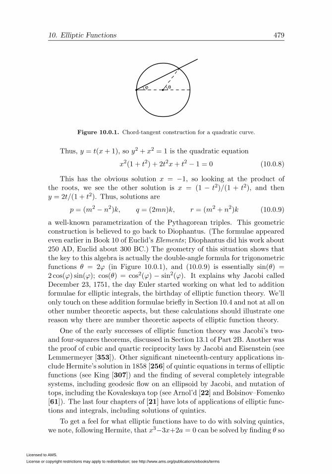
10. Elliptic Functions 479
ϕ θ
Figure 10.0.1. Chord-tangent construction for a quadratic curve.
Thus, y = t(x+ 1), so y2 + x2 = 1 is the quadratic equation
x2(1 + t2) + 2t2x+ t2 − 1 = 0 (10.0.8)
This has the obvious solution x = −1, so looking at the product ofthe roots, we see the other solution is x = (1 − t2)/(1 + t2), and theny = 2t/(1 + t2). Thus, solutions are
p = (m2 − n2)k, q = (2mn)k, r = (m2 + n2)k (10.0.9)
a well-known parametrization of the Pythagorean triples. This geometricconstruction is believed to go back to Diophantus. (The formulae appearedeven earlier in Book 10 of Euclid’s Elements ; Diophantus did his work about250 AD, Euclid about 300 BC.) The geometry of this situation shows thatthe key to this algebra is actually the double-angle formula for trigonometricfunctions θ = 2ϕ (in Figure 10.0.1), and (10.0.9) is essentially sin(θ) =2 cos(ϕ) sin(ϕ); cos(θ) = cos2(ϕ) − sin2(ϕ). It explains why Jacobi calledDecember 23, 1751, the day Euler started working on what led to additionformulae for elliptic integrals, the birthday of elliptic function theory. We’llonly touch on these addition formulae briefly in Section 10.4 and not at all onother number theoretic aspects, but these calculations should illustrate onereason why there are number theoretic aspects of elliptic function theory.
One of the early successes of elliptic function theory was Jacobi’s two-and four-squares theorems, discussed in Section 13.1 of Part 2B. Another wasthe proof of cubic and quartic reciprocity laws by Jacobi and Eisenstein (seeLemmermeyer [353]). Other significant nineteenth-century applications in-clude Hermite’s solution in 1858 [256] of quintic equations in terms of ellipticfunctions (see King [307]) and the finding of several completely integrablesystems, including geodesic flow on an ellipsoid by Jacobi, and nutation oftops, including the Kovaleskaya top (see Arnol’d [22] and Bolsinov–Fomenko[61]). The last four chapters of [21] have lots of applications of elliptic func-tions and integrals, including solutions of quintics.
To get a feel for what elliptic functions have to do with solving quintics,we note, following Hermite, that x3−3x+2a = 0 can be solved by finding θ so
Licensed to AMS.
License or copyright restrictions may apply to redistribution; see http://www.ams.org/publications/ebooks/terms

480 10. Elliptic Functions
that sin θ = a and noting that, by triple-angle formulae, the solutions of thecubic are 2 sin((2πj+θ)/3) for j = 0, 1, 2. Quintics use Jacobi θ functions andelliptic modular functions in place of sin and arcsin. Klein [312] developeda link of this approach to Galois theory by using the symmetry group of theicosahedron.
In the end, as a first pass, we’ll focus on double periodicity per se, butthese Notes should give the reader some flavor of why the full theory is somuch more and why it has led to multiple books.
10.1. A Warmup: Meromorphic Functions on C
Theorem 7.1.9 says that two meromorphic functions on a compact Riemannsurface, S, are determined up to a multiplicative constant by their zerosand poles (including their orders) and are also determined up to an additiveconstant by their principal parts. So it is a natural question to ask whatsets of zeros and poles and what principal parts can occur.
One obvious restriction comes from Theorem 7.1.10—the total numbersof zeros and of poles (counting orders) must agree. The main result in this
warmup section is that, for S = C, this is the only restriction.
Recall that a rational function is a ratio of polynomials Q(z)/P (z), thatwe suppose has no common zero. The following has been implicit in someplaces earlier in this book:
Theorem 10.1.1. Every meromorphic function on C is a rational function.The number of zeros and poles (counting orders) agree.
Remark. Of course, the converse of the first sentence is also true and thelast sentence follows from Theorem 7.1.10, but we provide a simple directproof.
Proof. Let f be the meromorphic function on C and {pj}N0j=1 the set of
poles in C, counting orders. Let
P (z) =
N0∏j=1
(z − pj) (10.1.1)
Then Q(z) ≡ f(z)P (z) is an entire function on C.Since f is meromorphic at ∞, near infinity, for some k,
|f(z)| ≤ C|z|k (10.1.2)
so, |Q(z)| ≤ C|z|k+N0 and Q is a polynomial by Theorem 3.1.9. Thus, f isrational.
If f = Q/P is rational, the order of the zero or pole at infinity is deg(P )−deg(Q) (with pole orders counted as negative numbers and f nonvanishing
Licensed to AMS.
License or copyright restrictions may apply to redistribution; see http://www.ams.org/publications/ebooks/terms

10.2. Lattices and SL(2,Z) 481
and regular at ∞ if this number is 0). Since deg(P ) counts the sum of theorders of poles in C and deg(Q) of the zeros, we get the claimed equality onthe total number of zeros and poles. �
Theorem 10.1.2. Let {zj}Nzj=1 and {pj}Np
j=1 be finite sequences of points
in C with pj �= zk for all j, k, and suppose Nz = Np. Then there exists
a rational function whose zeros (counting orders) is precisely {zj}Nzj=1 and
poles {pj}Np
j=1.
Proof. By renumbering, we can suppose for some N(0)z , N
(0)p that zj = ∞
for j ≥ N(0)z + 1 and zj �= ∞ for j ≤ N
(0)z , and similarly for the poles (by
hypothesis, either N(0)z = Nz or N
(0)p = Np or both).
f(z) =
∏N(0)z
j=1 (z − zj)∏N(0)z
j=1 (z − pj)(10.1.3)
has the required poles and zeros in C and the order of its pole or zeroat infinity is, by Np = Nz, precisely the number of times ∞ occurs inthe sets. �
Theorem 10.1.3. Let {pj}Np
j=1 be a set of distinct points in C and {Pj}Np
j=1
potential principal parts of a pole at pj. Then there exists a meromorphic
function, f , on C so that the poles and principal parts are precisely {pj}Np
j=1
and {Pj}Np
j=1.
Remark. The principal part at ∞ of a meromorphic function on C is thenegative terms in the Taylor series in z−1, so a polynomial in z with zeroconstant term.
Proof. Let Pj(z) = Pj(1/z − pj) if pj �=∞ and Pj(z) if pj =∞. Take
f(z) =
Np∑j=1
Pj(z) (10.1.4)
Since f(z)− Pj is analytic at pj , f has the requisite principal parts. �
10.2. Lattices and SL(2,Z)
Elliptic functions are left invariant by adding to their arguments elementsof a subset L ≡ {t} ⊂ C of those t with f(z + t) = f(z) for all z. Clearly,if t1, t2 ∈ L ⇒ t1 + t2 ∈ L and −t ∈ L. For f to be nonconstant, L cannothave finite limit points. If tn → t∞, tn+1 − tn → 0, so it suffices that 0 isnot a limit point. This leads to the natural definition:
Licensed to AMS.
License or copyright restrictions may apply to redistribution; see http://www.ams.org/publications/ebooks/terms

482 10. Elliptic Functions
Definition. A lattice, L ⊂ C, is a subset that obeys
(i) t1, t2 ∈ L ⇒ t1 − t2 ∈ L(ii) inft∈L, t �=0|t| > 0
In other words, a lattice is a discrete additive subgroup. We’ll always sup-pose L is nontrivial, that is, L has at least two (and so, an infinity of)points.
This section, as a preliminary, will study lattices in C and their geometry.We’ll begin by defining bases showing the existence of what we’ll call minimalbases. We’ll see the set of all bases with Im τ2/τ1 > 0 for a lattice, L, isnaturally a transitive homogeneous space for the group, SL(2,Z), and usethe existence of minimal bases to find a fundamental domain for the actionof SL(2,Z) on C+. There will be a subtle interplay between the group andthe set of lattices. Finally, we’ll study 1
2L ⊃ L and an associated naturalsubgroup, Γ(2), of SL(2,Z) and find a fundamental domain for it.
We begin by showing that every lattice as a group is isomorphic to Zor Z2.
Theorem 10.2.1. Let L be a lattice in C and pick
τ1 ∈ {t ∈ L | |t| = infs∈L\{0}
|s|} (10.2.1)
which is a nonempty set. Then, either
(i) L ⊂ Rτ1 = {xt1 | x ∈ R} (10.2.2)
in which case,
L = Zτ1 = {nτ1 | n ∈ Z} (10.2.3)
or
(ii) L �⊂ Rτ1
in which case, if
τ2 ∈ {t ∈ L \ Rτ1 | |t| = infs∈L\Rτ1
|s|} (10.2.4)
which is nonempty, then
L = Zτ1 + Zτ2 = {n1τ1 + n2τ2 | nj ∈ Z} (10.2.5)
and any t ∈ L has a unique representation n1τ1 + n2τ2.
Proof. Let R = inft∈L, t �=0|t| > 0, by hypothesis. If the set (10.2.1) wereempty, there must be tn ∈ L with |tn| > R but |tn| → R and then, bycompactness, distinct tn → t∞, which is forbidden since |t − s| ≥ R for allt, s ∈ L with t �= s.
Licensed to AMS.
License or copyright restrictions may apply to redistribution; see http://www.ams.org/publications/ebooks/terms

10.2. Lattices and SL(2,Z) 483
Suppose L ⊂ Rτ1. Then every t ∈ L is of the form xτ1 with x ∈ R. Ifx /∈ Z, {x}τ1 = t−[x]τ1 ∈ L and 0 < |{x}τ1| < |τ1| = R, which is impossible.Thus, L ⊂ Zτ1. Clearly, Zτ1 ⊂ L, so (10.2.3) holds.
If L �⊂ Rτ1, let R1 be the inf in the set in (10.2.4). Since points in L area distance at least R apart if there are k points in L ∩ D2R1(0), there are kdisjoint disks of radius R/2 in D2R1+R/2, so k ≤ ((2R1 +
12R)/(12R))2 <∞.
Since there are finitely many points in L ∩ D2R1 \ Rτ1 and there are somepoints (by definition of R1), there must be one of smallest norm, so the setin (10.2.4) is nonempty.
Since τ2 /∈ Rτ1, τ1 and τ2 are a vector space basis for C as a vector spaceover R, so any t ∈ L can be written
t = x1(t)τ1 + x2(t)τ2 (10.2.6)
Picking integers with |xj(t)− nj | ≤ 12 , we see
s ≡ t− n1τ1 − n2τ2 = y1τ1 + y2τ2 (10.2.7)
with |yj| ≤ 12 . If y2 �= 0, s ∈ L \ Rτ1 with
|s| < 12 |τ1|+
12 |τ2| ≤ |τ2| (10.2.8)
(10.2.8) is obvious if y1 = 0 and is true if y1 �= 0, since nonparallel vectorsobey a strict triangle inequality. This is a contradiction, so y2 ≡ 0. But then,since as above, L ∩Rτ1 = Zτ1, y1 = 0. We conclude s = 0 so t ∈ Zτ1 + Zτ2.
Uniqueness of representation follows from the fact that τ1 and τ2 arelinearly independent over R. �
We call L one-dimensional if L = Zτ1 and two-dimensional otherwise.Henceforth, we only consider the two-dimensional case. Two vectors, t1, t2,in L, a two-dimensional lattice, are called a basis of L if and only if
L = {n1t1 + n2t2 | n1, n2 ∈ Z} (10.2.9)
Since L �⊂ Rt1, we have that Im(t2/t1) �= 0. Clearly, if (t1, t2) are a basis, soare (±t1,±t2) for the four independent choices of ±. We can partly removethis multiplicity by demanding Im(t2/t1) > 0, which can be arranged ifnecessary by replacing t2 by −t2. We’ll call such a basis an oriented basisand τ = t2/t1, the ratio of the basis. If (τ1, τ2) is an oriented basis whichobeys (10.2.1) and (10.2.4), we call it a minimal basis.
SL(2,Z) is the set of elements in SL(2,C) with integral coefficients. Theinverse of such a matrix is again in SL(2,Z) by Cramer’s rule for the inverse.In addition, we note that if A ∈ GL(2,Z) with A−1 ∈ GL(2,Z), det(A) =±1, since det(A) det(A−1) = 1 but both have to be integers. Any A ∈hom(C2), the 2× 2 complex matrices, induces a map BA : (t1, t2)→ (s1, s2)
Licensed to AMS.
License or copyright restrictions may apply to redistribution; see http://www.ams.org/publications/ebooks/terms
484 10. Elliptic Functions
on pairs of vectors by
BA(t1, t2) = (a11t1 + a12t2, a21t1 + a22t2) (10.2.10)
Proposition 10.2.2. (a) BA maps L×L into L×L for any A ∈ hom(Z2),the 2× 2 matrices with integral coefficients.
(b) If t1, t2 is an oriented basis for L, then BA(t1, t2) = (s1, s2) is an ori-ented basis if and only if A ∈ SL(2,Z).
(c) Given any two oriented bases of L, (t1, t2) and (s1, s2), there is a uniqueA ∈ SL(2,Z) with
BA(t1, t2) = (s1, s2) (10.2.11)
Proof. (a) is obvious.
(b) By definition of basis, if (t1, t2) is a basis, then for any (s1, s2) ∈ L × Lcan be written (10.2.11) for A ∈ hom(Z2). If s1, s2 is also a basis, then(t1, t2) = BB(s1, s2) where B also has integrable elements. Thus, BA = �,so since det(A) det(B) ∈ Z, det(A) = ±1. But a simple calculation showsthat
Im
(s2s1
)=
det(A) Im( t2t1 )
|a11 + a12t2t1|2
(10.2.12)
so if both bases are oriented, det(A) > 0, that is, A ∈ SL(2,Z). Runningthese calculations backwards shows, conversely, that BA for A ∈ SL(2,Z)maps oriented bases to oriented bases.
(c) Since (s1, s2) and (t1, t2) are bases, there exist A,B with integral elementsso that BA(t1, t2) = (s1, s2) and BB(s1, s2) = (t1, t2). Thus, AB = �, sodet(A) = ±1 and (10.2.12) implies det(A) > 0, so A ∈ SL(2,Z). �
If A = ( a11 a12a21 a22 ) and
gA(z) =a22z + a21a12z + a11
(10.2.13)
(which, in terms of fA of Section 7.3, is fC with C = ( 0 ii 0 )A(
0 ii 0 )
−1), if(10.2.11) holds, and if τ = t2/t1, σ = s2/s1, then
σ = gA(τ) (10.2.14)
Thus, SL(2,Z) acts on the set of all bases in such a way that the inducedaction on basis ratios is by FLTs, albeit a conjugate of the “usual” action.
We want to ask what ratios arise for minimal bases. Define (see Fig-ure 10.2.1)
F int = {z ∈ C+ | |z| > 1, |Re z| < 12} (10.2.15)
C+ = {z ∈ C+ | |z| = 1, 0 ≤ Re z ≤ 12} (10.2.16)
C− = {z ∈ C+ | |z| = 1, −12 ≤ Re z ≤ 0} (10.2.17)
Licensed to AMS.
License or copyright restrictions may apply to redistribution; see http://www.ams.org/publications/ebooks/terms

10.2. Lattices and SL(2,Z) 485
Figure 10.2.1. The region F .
E± = {z ∈ C+ | |z| ≥ 1, Re z = ±12} (10.2.18)
F = F int ∪ C+ ∪ E+, F = F ∪ C− ∪ E− (10.2.19)
A special role is played by the single point in C+ ∩ E+, that is
ω0 =12 + i
√34 (10.2.20)
The lattice with τ1 = 1, τ2 = ω0 has a symmetry under rotations by 60◦.Notice that ω0 is a sixth root of unity. A less special role involves the pointin C+ ∩ C−, that is, τ = i. The lattice with τ1 = 1, τ2 = i has a symmetryunder 90◦ rotations.
Theorem 10.2.3. Let A ∈ SL(2,Z), τ, σ ∈ F with gA(τ) = σ. Then one ofthe following holds:
(i) A = ±�(ii) τ = σ = i; A = ±( 0 1
−1 0 )
(iii) τ = σ = ω0; A = ±( 0 1−1 1 ) or A = ±(−1 1
−1 0 )
In all cases, τ = σ.
Proof. Since τ = gA−1(σ), by interchanging τ and σ and replacing A byA−1, we can suppose Imσ ≥ Im τ . In this equivalence, it is important tonote that up to ±�, the A in (ii) is its own inverse and the A’s in (iii) areeach other’s inverse. Now, since det(A) = 1,
σ =a22τ + a21a12τ + a11
, Imσ =Im τ
|a12τ + a11|2(10.2.21)
Licensed to AMS.
License or copyright restrictions may apply to redistribution; see http://www.ams.org/publications/ebooks/terms
486 10. Elliptic Functions
so Imσ ≥ Im τ implies
|a12τ + a11|2 ≤ 1 (10.2.22)
This implies |a12| ≤ 1/|Im τ | ≤√
4/3 since the minimum value of Im τ
in F is at τ = ω0 with Im τ =√3/4. Thus, a12 = 0 or ±1. So long as we
multiply the possibilities for A by −1, we can suppose a12 = 0 or a12 = 1.
Case 1: a12 = 0. Then a11a22 = det(A) = 1, so a11 = a22 = ±1 and, by(10.2.21), σ = τ ± a21. Since F ∩ (F +n) = ∅ for n ∈ Z \ {0}, we must havea21 = 0, that is, A = ±�. So we have (i).
Case 2: a12 = 1, a11 �= 0. Then
1 ≥ |a11 +Re τ |2 ≥ (|a11 − 12 |)
2 (10.2.23)
so a11 = ±1 and so, |Im τ |2 ≤ 1 − 14 which implies τ = ω0 since the only
τ ∈ F with Im τ ≤√
3/4 is ω0. Thus, Re τ = 12 and (10.2.23) implies
a11 = −1. Thus, |a12τ + a11| = |ω0 − 1| = 1 and Imσ = Im τ , so σ = ω0
also. Thus,
a22ω0 + a21 = ω0(ω0 − 1) = ω30 = −1 (10.2.24)
so a22 = 0, a21 = −1, that is, A = (−1 1−1 0 ) and σ = τ = ω0, which is one of
the possibilities of (iii).
Case 3: a12 = 1, a11 = 0. Then det(A) = 1 implies a21 = −1 andσ = a22 − τ−1. (10.2.22) implies |τ | ≤ 1, so since τ ∈ F , |τ | = 1, so τ ∈ C+and −τ−1 ∈ C−. Only two pairs μ+ ∈ C+, μ− ∈ C− have μ+ − μ− ∈ Z.μ+ = μ− = i and a22 = 0 (which is when (ii) holds) or μ+ = ω0, a22 = 1and 1− ω−1
0 = ω0, which is the other possibility where (iii) holds. �
Theorem 10.2.4. (a) For any minimal basis of a lattice, L, the ratio τ liesin F .
(b) Every lattice has a minimal basis whose ratio lies in F .(c) If a lattice has two oriented bases whose ratios both lie in F , the ratios
are the same.(d) If a basis has a ratio in F , then it is a minimal basis.(d) Every τ ∈ F is the ratio of a minimal basis of some lattice.
Remark. Problem 1 will explore the number of distinct minimal bases alattice has.
Proof. (a) Let τ1, τ2 be a minimal basis with τ2/τ1 = τ . |τ2| ≥ |τ1| implies|τ | ≥ 1. Since it is oriented, Im τ > 0. Since (τ1, τ2 + τ1) is also a basis,|τ2 ± τ1| ≥ |τ2| ⇒ |1 ± τ |2 ≥ |τ |2 ⇒ 1 ± 2Re τ ≥ 0 ⇒ |Re τ | ≤ 1
2 . Thus,
τ ∈ {τ | |τ | ≥ 1, Im τ > 0, |Re τ | ≤ 12} = F .
(b) Let (τ1, τ2) be a minimal basis with ratio τ . If τ ∈ E−, (τ1, τ2+ τ1) is anoriented basis and |τ2 + τ1|/τ2 = |τ +1| = |τ | since τ ∈ E−, so (τ1, τ2 + τ1) is
Licensed to AMS.
License or copyright restrictions may apply to redistribution; see http://www.ams.org/publications/ebooks/terms

10.2. Lattices and SL(2,Z) 487
a basis with ratio 1+ τ ∈ E+. If τ ∈ C−, (τ2,−τ1) is an oriented basis, whichis also minimal (since |τ2| = |τ1|), and the ratio for (τ2,−τ1) is −τ−1 ∈ C+.Thus, if τ ∈ F \ F , there is also a minimal basis with ratio in F .
(c) Let (t1, t2) and (s1, s2) both be bases whose ratios τ, σ lie in F . Thenthere is A ∈ SL(2,C) so (s1, s2) = BA(t1, t2). Thus, σ = gA(τ), so byTheorem 10.2.3, σ = τ .
(d) Let (t1, t2) be the basis with ratio τ ∈ F . By the construction in theproof of (b), there is another oriented basis with |t′1| = |t1|, |t′2| = |t2|, andratio τ ′ ∈ F . By (b), there is a minimal basis (s1, s2) with ratio, σ, in F .Thus, by (c), τ = σ. Moreover, by Theorem 10.2.3, either the change ofbasis, A, is ±�, or A is one of the two special cases where all four latticevectors (t′1, t
′2, s1, s2) have the same length. Thus, t′ and so t is minimal.
(e) Let τ ∈ F . Let L = {n1+n2τ | n1, n2 ∈ Z}. 1, τ ∈ L are clearly a basis.Their ratio is in F , so it is a minimal basis. �
Definition. Let G be a group of analytic automorphisms of a region Ω ⊂ C.A fundamental domain, G, is a subset of Ω that contains exactly one pointof each orbit of G, that is, for all z ∈ Ω, there is a unique w ∈ G and someF ∈ G so F (w) = z.
Usually, one wants G to be connected and also that Gint = G.
Theorem 10.2.5. F is a fundamental domain for the action A �→ gA ofSL(2,Z) on C+.
Remark. Since there is T ∈ SL(2,Z) with fA = gTAT−1 so the orbits{fA(Tw) | A ∈ SL(2,C)} are the orbits {gA(w) | A ∈ SL(2,C}, F is also afundamental domain for the action A �→ fA.
Proof. Let τ ∈ C+. Let L = {n1 + n2τ | n1, n2 ∈ Z}. L is a lattice withbasis (1, τ). By Theorem 10.2.4, it has a minimal basis with ratio, σ, in Fso τ = gA(σ) for some A ∈ SL(2,C). So each orbit contains a point in F .Uniqueness follows from Theorem 10.2.3. �
The relation of the lattice 12L = {12z | z ∈ L} to L will play an important
role, especially in Section 10.6, and related to this is the subgroup of SL(2,C)
Γ(2) =
{(α βγ δ
) ∣∣∣∣ α, δ odd; β, γ even
}(10.2.25)
called the principal conjugacy subgroup of level 2. As a test, the readermight guess the answer to the question of what its index is as a subgroupof SL(2,Z), that is, how many left cosets it has. We’ll answer it shortly.
L is a subgroup of index 4 in 12L—its four cosets are naturally labeled ee,
eo, oe, and oo. For example, oe = {12(n1τ1 + n2τ2) | n1 odd and n2 even}.
Licensed to AMS.
License or copyright restrictions may apply to redistribution; see http://www.ams.org/publications/ebooks/terms

488 10. Elliptic Functions
If we pick a basis τ1, τ2 of L, SL(2,Z) acts on 12L by AA : 1
2L →12L by
AA(12 n1τ1 +
12 n2τ2) =
12 n1(a11τ1 + a12τ2) +
12 n2(a21τ1 + a22τ2) (10.2.26)
then each AA takes ee to ee, that is, AA maps L to L, and so it maps cosets
of L in 12L to (possibly distinct) cosets, that is, there is a map AA : 1
2L/L →12L/L by
AA([t]) = [AA(t)] (10.2.27)
Since
AA(12 n1τ1 +
12 n2τ2) =
12 τ1(a11n1 + a21n2) +
12 τ2(a12n1 + a22n2) (10.2.28)
we see a11n1+a21n2 ≡ n1 (mod 2), a21n1+a22n2 ≡ n2 (mod 2) for all n1, n2
if and only if all of a11− 1, a21, a21, a22− 1 are even, that is, A ∈ ker(AA) ≡{A | AA([t]) = [t] for all t} if and only if A ∈ Γ(2). Thus, SL(2,Z)/Γ(2)acts on 1
2L/L and this action is one-one. The image maps all map the coset[L] ≡ ee to itself and permute the other three cosets oo, oe, and eo in someway. A = ( 0 1
1 0 ) leaves oo fixed but permutes oe and eo, while by (10.2.28),A = ( 1 1
−1 0 ) maps oo to eo, eo to oe, and oe to oo. These two elements ofS3, the six-element permutation group on three objects, generate the whole
group, so Ran(AA) has six elements, that is, the index of Γ(2) in SL(2,Z)is six. Thus, we’ve proven that:
Theorem 10.2.6. Γ(2) has index 6 in SL(2,Z).
Now, let F be the set
F = {z | −1 < Re z ≤ 1; Im z > 0; |z − 12 | ≥
14 , |z +
12 | >
14} (10.2.29)
which we’ve seen in Section 8.3; see Figure 8.3.1.
Theorem 10.2.7. F is a fundamental region for the group Γ(2) under theaction gA of Γ(2).
Remark. In Section 8.3, we proved that F is a fundamental region forthe group of FLTs which were products of an even number of reflections in|z − 1
2 | =12 , in Re z = 0, and in Re z = 1. In Problem 2, the reader will
show this group is Γ(2) and so provide another proof of this theorem.
Proof. It’s proof by picture!
Figure 10.2.2 divides F in twelve regions, six shaded and six not. Thetwo regions labeled 1 and 7 form F . There are five elements, C2, . . . , C6,in SL(2,Z), one from each nontrivial coset of SL(2,Z)/Γ(2), that map region
1 to 2 – 6 and five different ones, C8, . . . , C12, that map 7 to 8 – 11 .Set C1 = C7 = �. Given any z ∈ C+, find B ∈ SL(2,C) with gB(z) ∈ F . If
in region 1 , find the one of C1, . . . , C6 so CjB ∈ Γ(2). Then gCjB(z) ∈ F ,
Licensed to AMS.
License or copyright restrictions may apply to redistribution; see http://www.ams.org/publications/ebooks/terms

10.2. Lattices and SL(2,Z) 489
1
2
3
4
5
6 7
8
9
10
11
12
�1 �1
20
1
21
Figure 10.2.2. Using F to cover ˜F .
showing each orbit intersects F and the uniqueness of the element of SL(2,Z)and that only one of CjB ∈ Γ(2) for j = 1, . . . , 6 imply uniqueness. �
We haven’t worried about proving proper counting of boundary points.We leave that to Problem 4.
Notes and Historical Remarks. The lattices associated with the sym-metry points τ = ω0 and τ = i have six-fold and four-fold rotational sym-metries. It is no coincidence that four and six occur and not, say, 10 or eight(because of τ → −τ symmetry, only even orders occur). For in the τ1, τ2basis, the implementation of the rotations lies in SL(2,Z), so their trace isin Z. But a rotation of angle at θ has trace 2 cos(θ). Since cos(θ) ∈ [−1, 1],this is in Z only for θ = 0, πj/3 (j = 1, . . . , 5), πj/2 (j = 1, 2, 3), so onlytwo-, three-, four-, six-fold symmetries occur.
These same arguments imply that the only elements of SL(2,Z) thathave a fixed point in C+ are of order two or three in PSL(2,Z) (as we’veseen, elements of Aut(D) with a fixed point in D are elliptic, so that is trueof C+). Note the special A’s in Theorem 10.2.3 are order four and six andinduce elements of PSL(2,Z) of order two and three.
One consequence of the theorem that a lattice is spanned by a two-element basis is that if a function has three periods that are independent inthat no nontrivial integral combination of them is zero, then f is constant
Licensed to AMS.
License or copyright restrictions may apply to redistribution; see http://www.ams.org/publications/ebooks/terms

490 10. Elliptic Functions
(see Problem 5). This result goes back to Jacobi at the dawn of the theoryof doubly periodic functions.
Problems
1. Let L be a lattice with minimal basis τ1, τ2 where τ = τ2/τ1 ∈ F .
(a) Prove that if τ ∈ F int, then only (τ1, τ2) and (−τ1,−τ2) are minimalbases.
(b) If τ ∈ E+ \ {ω0}, prove there are exactly four minimal bases ±(τ1, τ2)and ±(τ1, τ2 − τ1).
(c) If τ ∈ C+ \ {ω0}, prove there are exactly four minimal bases ±(τ1, τ2)and ±(τ2,−τ1).(d) If τ = ω0, prove there are exactly twelve minimal bases (τ1ω
�0, τ1ω
�+10 )
and (τ1ω�0, τ2ω
�+20 ) for � = 0, 1, . . . , 5.
(e) Prove that the number of minimal bases with ratio τ is two if τ �= i, ω0,four if τ = i, and six if τ = ω0.
2. This will lead you through a proof that Γ(2) is generated by ±( 1 20 1 )
and ( 1 02 1 ). Let ( a b
c d ) ∈ Γ(2) and let G be the subgroup generated by±τ = ±( 1 2
0 1 ) and σ = ( 1 02 1 ).
(a) Prove that if c = 0, then ( a bc d ) ∈ G.
(b) Let X = Γ(2) \G. Prove that x ∈ X and y ∈ G⇒ yx ∈ X.
(c) Suppose X is nonempty and x0 = ( a bc d ) ∈ X is chosen so that |c| is
minimal among x ∈ X, and among those x with this value of |c|, |a| isminimal. By considering τ±1x, prove that |a±2c| ≥ |a| or |a| ≤ |c|. Notethat, by (a), |c| ≥ 2, and by a odd, |a| ≥ 1. By considering σ±1x, provethat |c ± 2a| ≥ |c| or |c| ≤ |a|. Get a contradiction and conclude thatG = Γ(2).
(d) Prove that the group generated by even numbers of reflections inRe z = 0, Re z = 1, and |z − 1
2 | =12 is Γ(2).
3. Find explicit formulae for the SL(2,Z) matrices C1, . . . , C12 of the proofof Theorem 10.2.7.
4. Prove that boundary points are properly counted so that each orbit in
Γ(2) contains exactly one point of F . (Hint: You’ll need to treat ω0 andi differently from other points! Why?)
5. (a) If τ1, τ2 is a basis of a lattice, L, prove that if σ1, σ2 are any inde-pendent points in L (in that for no (m1,m2) ∈ Z2 other than (0, 0) ism1σ1 +m2σ2 = 0), then τ1 and τ2 are rational linear combinations of σ1and σ2.
Licensed to AMS.
License or copyright restrictions may apply to redistribution; see http://www.ams.org/publications/ebooks/terms

10.3. Liouville, Abel, and Jacobi 491
(b) Prove for any σ1, σ2, σ3 ∈ L, there are integers m1,m2,m3 not allzero so that m1σ1 +m2σ2 +m3σ3 = 0.
(c) If σ1, σ2, σ3 are three points in C independent over Z, prove that theintegral combinations of σ1, σ2, σ3 are dense in C. (This is a result ofJacobi.)
10.3. Liouville’s Theorems, Abel’s Theorem, and Jacobi’sConstruction
In this section, we’ll prove a series of four theorems of Liouville that delineatewhat possibilities there are for elliptic functions and state, but only beginthe proof of the basic existence theorems that say the necessary conditionsfound by Liouville are also sufficient. We’ll reduce, following Jacobi, theexistence theorems to the existence of a single nonelliptic function withsuitable properties. Later, once in Section 10.4 and once in Section 10.5,we’ll construct the required function in two ways. We begin by statingLiouville’s theorems together. f will be nonconstant and have periods τ1, τ2with Im(τ2/τ1) > 0, {zj}Nz
j=1 and {pj}Np
j=1 will be its zeros and poles in
{xτ1 + yτ2 | 0 ≤ x < 1, 0 ≤ y < 1} (10.3.1)
counting multiplicity. (10.3.1) is called the fundamental cell or fundamentalperiod parallelogram; see Figure 10.3.1.
τ
τ1
τ +τ1 2
0
2
Figure 10.3.1. A fundamental cell.
Theorem 10.3.1 (Liouville’s First Theorem). f has poles, that is, Np ≥ 1.
Theorem 10.3.2 (Liouville’s Second Theorem).
Np = Nz (10.3.2)
Theorem 10.3.3 (Liouville’s Third Theorem). The sum of the residues atthe poles is zero, that is,
Np∑j=1
Res(f ; pj) = 0 (10.3.3)
Corollary 10.3.4. Np ≥ 2
Licensed to AMS.
License or copyright restrictions may apply to redistribution; see http://www.ams.org/publications/ebooks/terms
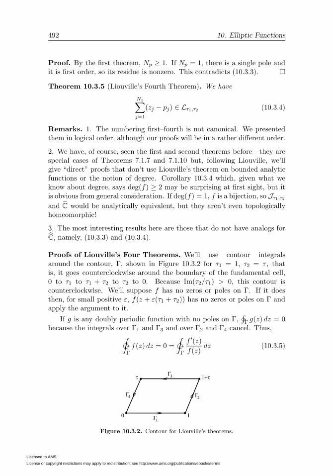
492 10. Elliptic Functions
Proof. By the first theorem, Np ≥ 1. If Np = 1, there is a single pole andit is first order, so its residue is nonzero. This contradicts (10.3.3). �
Theorem 10.3.5 (Liouville’s Fourth Theorem). We have
Nz∑j=1
(zj − pj) ∈ Lτ1,τ2 (10.3.4)
Remarks. 1. The numbering first–fourth is not canonical. We presentedthem in logical order, although our proofs will be in a rather different order.
2. We have, of course, seen the first and second theorems before—they arespecial cases of Theorems 7.1.7 and 7.1.10 but, following Liouville, we’llgive “direct” proofs that don’t use Liouville’s theorem on bounded analyticfunctions or the notion of degree. Corollary 10.3.4 which, given what weknow about degree, says deg(f) ≥ 2 may be surprising at first sight, but itis obvious from general consideration. If deg(f) = 1, f is a bijection, so Jτ1,τ2
and C would be analytically equivalent, but they aren’t even topologicallyhomeomorphic!
3. The most interesting results here are those that do not have analogs for
C, namely, (10.3.3) and (10.3.4).
Proofs of Liouville’s Four Theorems. We’ll use contour integralsaround the contour, Γ, shown in Figure 10.3.2 for τ1 = 1, τ2 = τ , thatis, it goes counterclockwise around the boundary of the fundamental cell,0 to τ1 to τ1 + τ2 to τ2 to 0. Because Im(τ2/τ1) > 0, this contour iscounterclockwise. We’ll suppose f has no zeros or poles on Γ. If it doesthen, for small positive ε, f(z + ε(τ1 + τ2)) has no zeros or poles on Γ andapply the argument to it.
If g is any doubly periodic function with no poles on Γ,�Γ g(z) dz = 0
because the integrals over Γ1 and Γ3 and over Γ2 and Γ4 cancel. Thus,‰Γf(z) dz = 0 =
‰Γ
f ′(z)
f(z)dz (10.3.5)
τ 1+τ
0 1
Γ3
Γ2Γ4
Γ1
Figure 10.3.2. Contour for Liouville’s theorems.
Licensed to AMS.
License or copyright restrictions may apply to redistribution; see http://www.ams.org/publications/ebooks/terms

10.3. Liouville, Abel, and Jacobi 493
By the residue calculus, the integral on the left is the left side of (10.3.3),proving the third theorem; and by the argument principle, the integral onthe right is 2πi(Nz −Np), proving the second theorem.
The second theorem implies the first, for since f is nonconstant, f(z)−ahas isolated zeros for any a, soNz(f−a) = Np(f−a) impliesNp �= 0. Indeed,this argument shows that Nz(f − a) is constant for all a, that is, reprovesthe constancy of degree.
(10.3.4) is the most subtle. We consider
Q =1
2πi
‰Γzf ′(z)
f(z)dz (10.3.6)
On the one hand, by the fact that f ′/f has poles exactly at the zj and pjwith residues ± (the order of zeros or poles)
Q =∑j
(zj − pj)
There is no cancellation between Γ1 and Γ3 and Γ2 and Γ4; f ′(z +τj)/f(z + τj) = f ′(z)/f(z) but the z + τj doesn’t cancel z but leaves τj , so
Q = − τ22πi
ˆΓ1
f ′(z)
f(z)dz +
τ12πi
ˆΓ2
f ′(z)
f(z)dz (10.3.7)
Now, 12πi
´Γ1
f ′/f dz is the change of the argument of f from 0 to 1.
Since f(0) = f(1), f [Γ1] is a closed curve and the integral is its windingnumber about 0, that is, the integral is an integer, −n2. Similarly, thesecond integral in (10.3.7) is an integer, n1, so
Q = n1τ1 + n2τ2 (10.3.8)
�
These theorems place two restrictions, namely, (10.3.2) and (10.3.4) onthe zeros and poles, and one, namely, (10.3.3) on the principal parts. Thenext results say these are the only restrictions:
Theorem 10.3.6 (Abel’s Theorem). Let {zj}Nzj=1 and {pj}Nz
j=1 be two col-lections of points in the fundamental cell of a lattice Lτ1,τ2 with zj �= pkfor all j, k. Then a necessary and sufficient condition for there to exist adoubly periodic function with period lattice Lτ1,τ2 with precisely those zerosand poles in the fundamental cell is that (10.3.2) and (10.3.4) hold.
Theorem 10.3.7 (Principal Part Theorem). Let {pj}Np
j=1 be a finite collec-
tion of distinct points in the fundamental cell and {Pj(z)}Np
j=1 a collection of
Licensed to AMS.
License or copyright restrictions may apply to redistribution; see http://www.ams.org/publications/ebooks/terms

494 10. Elliptic Functions
nonzero polynomials with Pj(0) = 0. Then a necessary and sufficient con-dition for there to exist a doubly periodic function with period lattice Lτ1,τ2
with precisely these poles and principal part Pj(1/(z − pj)) at pj is that
Np∑j=1
P ′j(0) = 0 (10.3.9)
Remarks. 1. It is not claimed that there couldn’t be a larger period lattice;indeed, if the zeros and poles are invariant under adding τj/2, the periodlattice will include L 1
2τ1,
12τ2.
2. By Theorem 7.1.9, these functions are unique up to one overall constant.
3. Of course, all the zeros and poles are {zj + t}Nzj=1, t∈L and {pj + t}Np
j=1, t∈L.
4. (10.3.9) is just (10.3.3).
5. We use Np in the second theorem because there, {pj}Np
j=1 are distinct,
that is, multiplicity is encoded in the deg(Pj), not in the set of {pj}Np
j=1.
6. The fact that Np ≥ 2 is forced by Abel’s theorem, because if z, p are inthe fundamental cell and z �= p, then z − p /∈ L.
How might one go about constructing such a set of functions? Supposewe could find a doubly periodic analytic function, g, with a single zero inthe fundamental cell at z = 0. Of course, such functions do not exist! Butignore that for a moment. Then
f(z) =
∏Nzj=1 g(z − zk)∏Np
k=1 g(z − pk)(10.3.10)
is doubly periodic and has precisely the right zeros and poles. Of course,that would be too good since it violates both (10.3.2) and (10.3.4)!
For f to be doubly periodic, it isn’t necessary that g be doubly periodic.Suppose instead that
g(z + τj) = eαjg(z) (10.3.11)
for constants eα1 , eα2 . g(0) = 0 still forces g(t) = 0 for all t ∈ L. Then f(z)will obey f(z + τj) = f(z) so long as Np = Nz. For the constants cancel inthe ratio.
It isn’t quite obvious we can’t arrange (10.3.11). After all,
g(z) = C1eC2z (10.3.12)
does obey (10.3.11), but it doesn’t have the required zero. Again, it wouldbe too good if this g existed since it could produce f ’s, violating (10.3.4). Infact (see Problem 1), (10.3.12) are the only functions that obey (10.3.11).
Licensed to AMS.
License or copyright restrictions may apply to redistribution; see http://www.ams.org/publications/ebooks/terms

10.3. Liouville, Abel, and Jacobi 495
But we’ve made some progress. Suppose, instead, that for someα1, α2, ω1, ω2 ∈ C, g obeys
g(z + τj) = eαj+ωjzg(z) (10.3.13)
If∑Nz
j=1(zj − pj) = 0, then, in fact, g given by (10.3.10) will be doubly
periodic since, if (10.3.13) holds,
Nz∏k=1
g(z + τj − zk) = eαjNzeωj(∑Nz
k=1 zk)Nz∏k=1
g(z − zk) (10.3.14)
But what can we do if Nz = Np and∑Nz
j=1(zj−pj) ≡ t0 ∈ L but is not zero?
Define
z1 = z1 − t0, zj = zj , j = 2, . . . , Nz; pj = pj , j = 1, . . . , Nz
(10.3.15)
and g(z − zj) has zeros precisely at {zj + t}Nzt∈L = {zj + t}Nz
t∈L since t0 ∈ L.Thus,
f(z) =
∏Nzj=1 g(z − zj)∏Nzj=1 g(z − pj)
(10.3.16)
is doubly periodic with the right zeros and poles. We have thus proven:
Theorem 10.3.8 (Jacobi’s Construction). If there exists an entire analyticfunction, g, obeying (10.3.13) for some α1, α2, ω1, ω2, and if the only zeroof g in the unit cell is at z = 0, then (10.3.16) solves the existence part ofAbel’s theorem and proves that part of Theorem 10.3.6.
Of course, Liouville’s theorems include the other half.
We’ll construct the required g twice: in the next section as a Weierstrassproduct (calling g, σ) and in the section after that, using Jacobi’s thetafunctions (calling g, θ). g is not unique (see Problem 5) and, indeed, the ω’sfor σ and θ are different.
As an extra bonus, the existence of g also proves Theorem 10.3.7.
Proof of Theorem 10.3.7 if g exists. Let
h1(z) =g′(z)
g(z); hn(z) = −
1
n− 1
d
dzhn−1(z), n = 2, 3, . . . (10.3.17)
Then, since g(z) vanishes to first order at z = 0, h1(z) =1z +O(1) at z = 0,
and then, by induction,
hn(z) =1
zn+O(1) (10.3.18)
since (h1(z)− 1z ) is analytic at z = 0.
Licensed to AMS.
License or copyright restrictions may apply to redistribution; see http://www.ams.org/publications/ebooks/terms

496 10. Elliptic Functions
Moreover, by (10.3.13),
h1(z + τj) = h1(z) + ωj , hn(z + τj) = hn(z) n ≥ 2 (10.3.19)
where the second equation holds by induction. Write
Pk(z) =
�k∑m=1
akmzm (10.3.20)
By (10.3.18),
f(z) =∑km
akmhm(z − zk) (10.3.21)
has the requisite principal parts.
Since (10.3.9) says that∑
k ak1 = 0, we have that∑k,�
aklh�(z + τj − zk) =∑k,�
aklh�(z − zk) + τj∑k
ak1
=∑k,�
aklh�(z − zk)
so f is doubly periodic. �
The doubly periodic functions, f , for Lτ1,τ2 that one constructs from geither have second derivatives (e.g., h1 = (g′/g)′) or since deg(f) ≥ 2, atotal of four g’s. But one can construct doubly periodic functions from onlytwo g’s but with periods, τ1 and 2τ2. Since the fundamental cell is now twiceas big, in that cell, one has two zeros and two poles. The functions will beantiperiodic when only τ2 is added, so in the fundamental cell for Lτ1,2τ2 ,there will be zeros at 0, τ2 and poles at z0, z0 + τ2. For this to obey (10.3.4)for Lτ1,2τ2 , we will need 2z0 ∈ Lτ1,2τ2 , so we’ll take z0 = τ1/2. Thus, wewant a ratio g(z)/g(z + τ1/2) with a phase adjustment. We’ll suppose
g(−z) = −g(z) (10.3.22)
By Problems 3 and 5, this can always be arranged if any g obeying (10.3.13)exists. When (10.3.22) holds, we have that (Problem 3)
g(z + τj) = −eωj(z+τj/2)g(z) (10.3.23)
Here is the result:
Theorem 10.3.9. Let g obey (10.3.13) and (10.3.22). Define for j = 1, 2,
gj(z) = e−ωjz/2g
(z +
τj2
)(10.3.24)
Then with τj = τ3−j for j = 1, 2, the function
fj(z) =g(z)
gj(z)(10.3.25)
Licensed to AMS.
License or copyright restrictions may apply to redistribution; see http://www.ams.org/publications/ebooks/terms

10.3. Liouville, Abel, and Jacobi 497
has poles in τj/2 + Lτ and zeros in Lτ and obeys
fj(z + τj) = fj(z), fj(z + τj) = −fj(z) (10.3.26)
Proof. Problem 6 proves (10.3.26). �
One way of understanding the phase in (10.3.24) is to plug z − τj/2 forz in(10.3.23) to see
g
(z +
τj2
)e−ωjz = g
(z − τj
2
)(10.3.27)
so
g2j (z) = g
(z +
τj2
)g
(z − τj
2
)(10.3.28)
and
fj(z)2 =
g(z)2
g(z +τj2 )g(z −
τj2 )
is the proper choice (using a shift like in (10.3.16) to arrange∑
j zj− pj = 0)
to get an elliptic function with poles at 12τj + Lτ and zeros at Lτ .
Theorem 10.3.9 is not only interesting from an abstract point of view,but will be used for our construction of the Jacobi elliptic functionssn(z), cn(z), dn(z) in Section 10.5. In that regard, we note that τ1, τ2 can bereplaced by any basis s1, s2 with Im(s2/s1) > 0 (since that is all we use forτ2/τ1 and g obeys (10.3.13) for τ1, τ2 if and only if it obeys it for s1, s2 withdifferent αj , ωj). In particular, if
g3(z) = e−(ω1+ω2)z/2g
(z +
τ1 + τ22
)(10.3.29)
then
f3(z) =g(z)
g3(z)(10.3.30)
has
f3
(z +
τ1 + τ22
)= f3(z), f3(z + τ1) = −f3(z) (10.3.31)
since (τ1, τ1 + τ2) is also a basis.
Notes and Historical Remarks. While Liouville’s results are natural aspart of a pedagogic presentation, they not only have much less mathematicaldepth than the work of Abel, Jacobi, and Weierstrass, but had much lesshistorical significance. Indeed, as explained in the Notes to Section 3.1, whileLiouville discussed this work already in 1844 (almost twenty years after thework of Abel and Jacobi), it was only published in 1880 [64].
Abel and his contemporaries would certainly not recognize what we (andothers) call Abel’s theorem. Abel was studying elliptic integrals, notably the
Licensed to AMS.
License or copyright restrictions may apply to redistribution; see http://www.ams.org/publications/ebooks/terms

498 10. Elliptic Functions
lemniscate integral´ x0 (1− y4)−1/2 dy = u and made the critical observation
that the inverse function F (u) = x was, as a function of a complex variable,doubly periodic [2]. More generally, he looked at
´ xx0
R(z, w) dz where R
is a rational function and (z, w) obeys a polynomial equation P (z, w) = 0.These are now called abelian integrals (some authors require deg(P ) > 4while others include elliptic integrals among the Abelian integrals). Unlikethe elliptic case, this integral may not define a one-one multivalued map ofx to u so there is not an inverse function, but the integral is still multiplevalued with periods. Abelian integrals provide existence results on what areessentially meromorphic functions on certain Riemann surfaces, so the nameAbel’s theorem to the more general result (see Section 11.6) is appropriate,albeit the form and language we use here is much more modern.
In his major work on elliptic functions [280], Jacobi constructed ellipticfunctions as ratios of products of certain nonelliptic functions which obey(10.3.13), so the name we give Theorem 10.3.8 is appropriate. Jacobi’sconstruction is described in bonus Section 10.5. The Notes to that sectionand to Section 10.4 say more about the historical context of the work ofAbel and Jacobi, and the Notes to Section 10.5 include a capsule biographyof Jacobi.
Functions obeying (10.3.13) are sometimes called theta functions. We’llreserve that name for what is often called Jacobi’s theta function after thefunctions Jacobi used in his later work (a slight variant on his first thetafunctions). We will sometimes refer to “general theta functions” for func-tions obeying (10.3.13). The term quasi-elliptic (or even quasi-periodic, aterrible name, given its use for something very different; see Section 6.6 ofPart 4) is sometimes used for functions obeying (10.3.13)) or ones like h1 of(10.3.17) that are doubly periodic up to some simple “error term.”
The term Legendre relations (see Problem 2) is based on the special casehe proved in his work on elliptic functions [350, 351]; see Problem 13 ofSection 10.5. They were generalized to the general doubly periodic case byWeierstrass in his first work on elliptic integrals [583] and are sometimescalled the Legendre–Weierstrass relations.
Niels Henrik Abel (1802–29) was a Norwegian mathematician whose lifewas so melodramatic that were it a Hollywood movie, it would be dismissedas too tragic to be true! Among other aspects, his father, like Euler’s, aminister, and family were adversely impacted by fallout from the Napoleonicwars (specifically, a side conflict between England and Denmark), his finalillness was precipitated by a trip through the snow to his fiancee, and theletter informing him that he finally had a position as a professor arrivedtwo days after his death (like that of Riemann) from a lung ailment, inhis case, consumption. A year after he was unable to find employment, he
Licensed to AMS.
License or copyright restrictions may apply to redistribution; see http://www.ams.org/publications/ebooks/terms
10.3. Liouville, Abel, and Jacobi 499
not only had that offer, but a posthumous grand prize (jointly with Jacobi)from the French Academy. Earlier, Cauchy lost a manuscript that Abelhad submitted to the French Academy. (Galois also had a manuscript lostthrough a combination of actions by Cauchy and Fourier!) See [11, 528,529] for more on Abel’s life.
Abel’s first great work showed the impossibility of solving quintics interms of radicals, and eventually led to the notion of group—“abeliangroups” comes from this work. His celebrated memoire on elliptic func-tions, as we’ve noted, found the double periodicity and, in more generalcontexts, abelian integrals, abelian functions, and abelian periods. Livio[364] has an interesting biography in his book. Pesic [427] describes Abel’sproof for the insolvability of the quintic by radicals.
Joseph Liouville (1809–82) was a French mathematician who was ac-tive in the political turmoil around 1848, including an elective office. Hiscontributions include not only his results on elliptic functions but also theconstruction of the first transcendental numbers (e.g.,
∑∞n=1 10
−n!, some-times called Liouville’s constant; see Problem 6 of Section 5.4 of Part 1),important contributions to mechanics (his result on constancy of phase spacevolumes and on completely integrable systems including the introduction ofaction-angle variables), and his work with Sturm on ordinary differentialequations and their eigenfunction expansions (see Section 3.2 of Part 4) andthe Liouville–Green approximation (see Section 15.5 of Part 2B). He is alsonoteworthy for appreciating and publicizing Galois’ work ten years afterGalois’ death. Liouville served as a member of the moderate republicanmajority of the National Assembly in 1848 but was defeated for reelectionbecause he was too moderate for the electorate after the revolution of thatyear. Lutzen [370] has a biography of Liouville.
Liouville was a mentor to Charles Hermite (1822–1901) who (see Bel-hoste [40]) seems to have been the first to make systematic use of the Cauchyintegral theorem in the study of elliptic functions.
Problems
1. Suppose g is an entire function that obeys (10.3.11).
(a) Prove that g′/g is doubly periodic.
(b) Prove that g′/g is constant. (Hint: Since g has no poles, what do youknow about the residues of g′/g?)
(c) Prove g has the form (10.3.12).
2. Suppose that g obeys (10.3.13) and has a single zero in the unit cell.By considering
�(g′/g) dz around a Liouville contour, prove the Legendre
Licensed to AMS.
License or copyright restrictions may apply to redistribution; see http://www.ams.org/publications/ebooks/terms

500 10. Elliptic Functions
relation (see also Problem 13 of Section 10.5)
ω1τ2 − ω2τ1 = 2πi (10.3.32)
3. Let g be entire and obey (10.3.13).
(a) Prove that
g(z − τj) = e(ωjτj−αj)−ωjzg(z) (10.3.33)
(b) Let h(z) = g(z)/g(−z). Prove that
h(z + τj) = e2αj−ωjτjh(z) (10.3.34)
(c) If g(−z) = −g(z), prove that
g(z + τj) = −eωj(z+τj/2)g(z) (10.3.35)
(Hint: Prove first (10.3.35) holds where − is a priori ±1 and then lookat z = −τj/2.)(d) Returning to general g, suppose the only zeros of g occur at z ∈ L.Prove that h(z) = g(z)/g(−z) obeys h(z) = ebz for some b, and then
that g(z) = e−bz/2g(z) has g(−z) = ±g(z), and that if the zeros are alsosimple, that g(−z) = −g(z). (Hint: Prove that h is entire and doublyperiodic.)
4. Let g, g obey (10.3.13), be entire, and both have only simple zeros and
exactly at z ∈ L. Prove that g(z) = eaz2+bz+cg(z) for some a, b, c. (Hint:
Prove that if h = g/g, then (h′/h)′′ is doubly periodic.)
5. Let g obey (10.3.13). Let g(z) = eaz2+bz+cg(z).
(a) Prove g also obeys a formula like (10.3.13) with
αj = αj + aτ2j + bτj (10.3.36)
ωj = ωj + 2aτj (10.3.37)
(b) Prove if there is an entire g that obeys (10.3.15), there is always asecond g with g(−z) = −g(z), ω1 = 0, and ω2 = −2πi/τ1.(c) Prove that α1, α2 can be picked (they are each only determinedmod 2πi) so that
α1τ2 − α2τ1 =12 (ω2 − ω1)τ1τ2 + iπ(τ2 − τ1) (10.3.38)
6. Let g be an entire function obeying (10.3.13) and g(z) = −g(−z) so(10.3.35) holds. Fix a, b ∈ C and define
ga,b(z) = ebzg(z + a) (10.3.39)
Licensed to AMS.
License or copyright restrictions may apply to redistribution; see http://www.ams.org/publications/ebooks/terms

10.4. Weierstrass Elliptic Functions 501
(a) Prove that
ga,b(z + τj) = −eaωj+bτjeωj(z+τj/2)ga,b(z) (10.3.40)
(b) Let
ha,b(z) =g(z)
ga,b(z)(10.3.41)
Prove that
ha,b(z + τj) = e−(aωj+bτj)ha,b(z) (10.3.42)
(c) Pick a = τ1/2, b = −ω1/2. Prove that
ha,b(z + τ1) = ha,b(z), ha,b(z + τ2) = −ha,b(z) (10.3.43)
(Hint: Use Problem 2.)
7. Fix p1, . . . , p� in the fundamental cell. Let V (p1, . . . , p�;n1, . . . , n�) fornj ≥ 1 be the vector space of all elliptic functions whose only poles are
at {pj}�j=1 with order at most nj at pj . Prove that
dim(V (p1, . . . , p�;n1, . . . , n�)) =�∑
j=1
nj (10.3.44)
(Hint: Don’t forget to include the constant functions. (10.3.44) is theRiemann–Roch theorem for genus 1.)
10.4. Weierstrass Elliptic Functions
We’ll begin this section by finding a g that completes the proof of Abel’stheorem begun in the last section. The function g has to obey (10.3.13) andhave a zero at z = 0 and so at all z ∈ L. Since this is the only zero in thefundamental cell, the points in L are the only zeros in C. We know fromChapter 9 how to construct functions with prescribed zeros as products ofWeierstrass factors (see the definition of En(z) in (9.4.2)). Such factors don’tautomatically obey (10.3.13), but if E2 works (and it does), the quadraticexponential and the fact that the difference of a quadratic and its translate islinear is suggestive that (10.3.13) will hold. So we’ll begin with implementingthis idea—to define the Weierstrass σ-function, and so implement a generalformula for elliptic functions in terms of σ and its translates.
Then we’ll study the ℘-function, the simplest doubly periodic functionformed from σ via
℘ = −(σ′
σ
)′(10.4.1)
This ℘-function will be the star of this section and, in many ways, thechapter—we’ll reformulate the form of general elliptic functions in terms of
Licensed to AMS.
License or copyright restrictions may apply to redistribution; see http://www.ams.org/publications/ebooks/terms

502 10. Elliptic Functions
℘ and ℘′, prove a cubic differential equation for ℘, and so relate ℘ to ellipticintegrals and to elliptic curves, and state general addition formulae for ℘.
Two preliminary remarks on the choice of periods: The first involvesscaling. If λ ∈ C and
τ1 = λτ1, τ2 = λτ2 (10.4.2)
and f and g are functions on C related by
f(z) = g(λz) (10.4.3)
then
f(z + τj) = g(λz + τj) (10.4.4)
so (10.4.3) sets up a one-one correspondence between elliptic functions fwith periods τj and g with periods τj . We will often pick λ = τ−1
1 , thatis, after dropping the tilde, we’ll consider the case where the periods are 1and τ ∈ C+. We note that in specific situations, one wants to multiply byconstants in (10.4.4). For example, the ℘-function is normalized by ℘(z) =1/z2 +O(1) near z = 0, so making τj-dependence explicit, what we have is
℘(z | τ1 τ2) = λ2℘(λz | λτ1 λτ2) (10.4.5)
with an extra λ2.
The other remark concerns the convention about how one labels the ba-sis of the period lattices. We will take τ1 and τ2 as the basis for the periodlattice. There is another convention that uses 2τ1 and 2τ2 (or 2ωj) for thebasis. A variant uses 2τ1 and 2τ3 (and defines τ2 = τ1 + τ3). This basisis chosen because 1
2Lτ1,τ2 is important, so where we use 12τj below, those
using the other convention can use τj . Historically, the 2τj convention wasalmost universally used a hundred years ago. The overwhelming majority ofrecent general complex analysis texts use our convention (exceptions includeMarkushevich [372] and Segal [514]), but books specializing on elliptic func-tions are split, with the 2τj convention in a slight majority. I’ve no doubtmany of their authors, thinking of the traditions of their specialty, rail aboutthe barbarians who use our τj convention. In any event, the reader shouldbe aware of the differing conventions.
Since our basic function is going to be zero on L, we need to know aboutthe index of convergence of these zeros:
Lemma 10.4.1. We have that
α(|τ21 |+ |τ2|2)(n21 + n2
2) ≤ |n1τ1 + n2τ2|2 ≤ (|τ1|2 + |τ2|2)(n21 + n2
2) (10.4.6)
where
α =Im(τ2)
1 + |τ |2 , τ =τ2τ1
(10.4.7)
Licensed to AMS.
License or copyright restrictions may apply to redistribution; see http://www.ams.org/publications/ebooks/terms

10.4. Weierstrass Elliptic Functions 503
Remark. The upper bound also comes from the Cauchy–Schwarz inequal-ity.
Proof. Let τ1 = 1, τ2 = τ . Let A = ( 1 Re τRe τ |τ |2 ). Then
|n1τ1 + n2τ2|2 = (n1n2)A
(n1
n2
)(10.4.8)
Tr(A) = 1 + |τ |2, det(A) = |Im τ |2. Since both are positive, A is positive,so the two eigenvalues, λ− ≤ λ+, obey λ+ ≤ Tr(A) and λ− = det(A)/λ+ ≥|Im τ |2/Tr(A).
We thus have (10.4.6) if τ1 = 1, τ2 = τ . Since everything scales quadrat-ically under τ1 → λτ1, τ2 → λτ2, we get the result in general. �Proposition 10.4.2. For any two-dimensional lattice, L, we have that∑
t∈L\{0}|t|−α <∞ (10.4.9)
if and only if α > 2.
Remark. See Problems 1 and 2 for alternate proofs.
Proof. For α = 2, we have by (10.4.6) that∑t∈L\{0}
|t|−2 ≥ C∑
(n1,n2) �=0
(n21 + n2
2)−1
≥ 8C∞∑
n1=1
n1∑n2=1
(2n21)
−1
= 8C∞∑
n1=1
12 n
−11
=∞proving divergence if α ≤ 2.
For α > 2, again using (10.4.6),∑t∈L\{0}
|t|−2 ≤ C∑
(n1,n2) �=0
(n21 + n2
2)−α/2
≤ 4C∞∑n=1
n−α + 4C∑
n1,n2≥1
(2n1n2)−α/2
≤ 4C∞∑n=1
n−α + 4C
( ∞∑n=1
n−α/2
)2
<∞by the integral test. We used here that n2
1 + n22 ≥ 2n1n2. �
Licensed to AMS.
License or copyright restrictions may apply to redistribution; see http://www.ams.org/publications/ebooks/terms

504 10. Elliptic Functions
We define the Eisenstein series, Sk(L), for k ≥ 3 by
Sk(L) =∑
t∈L\{0}t−k (10.4.10)
For k odd, Sk = 0, since then (−t)−k = −(t)−k. So we’ll mainly look at keven. When L = {n+mτ}n,m∈Z, we write Sk(τ).
By Proposition 10.4.2, we cannot use E1, but we can use E2. We thusdefine the Weierstrass sigma-function,
σ(z | τ1 τ2) = z∏
t∈Lτ1,τ2\{0}E2
(z
t
)(10.4.11)
where E2 is the Weierstrass factor E2(z) = (1−z)e(z+z2/2). By the estimate(9.4.3), we get the first sentence in
Theorem 10.4.3. The product in (10.4.11) converges uniformly and abso-lutely on compacts of C to an entire function of order 2. We have that
σ(−z | τ1 τ2) = −σ(z | τ1 τ2) (10.4.12)
Moreover, for suitable ω1, ω2,
σ(z + τj | τ1 τ2) = −eωj(z+τj/2)σ(z | τ1 τ2) (10.4.13)
Also,
σ(0) = 0, σ′(0) = 1 (10.4.14)
Proof. As noted, (9.4.3) implies convergence and analyticity. (10.4.12) fol-lows from E2(−z/− t) = E2(z/t) and −L \ {0} = L \ {0}. Since E2(0) = 1,we have (10.4.14).
We turn to (10.4.13). Fix j = 1 or 2. For t ∈ L, we let
gt(z) =
⎧⎪⎪⎨⎪⎪⎩E2(
z+τjt+τj
)/E2(z/t), t �= 0,−τjE2(
z+τjτj
)/z, t = 0
(z + τj)/E2(z/− τj), t = −τjSince 1 − (z + τj)/(t + τj) = [t/(t + τj)](1 − z/t), we see each gt(z) =exp(second degree polynomial). By the absolute convergence of the prod-uct, which lets us rearrange terms,
σ(z + τj)
σ(z)=∏t∈L
gt(z) = exp(second degree polynomial) (10.4.15)
The point, of course, is to prove that the quadratic terms cancel, and onecan do this by controlling the boundary terms in the sum (see Problem 3),but instead we’ll use a trick.
Licensed to AMS.
License or copyright restrictions may apply to redistribution; see http://www.ams.org/publications/ebooks/terms

10.4. Weierstrass Elliptic Functions 505
Let ζ, the Weierstrass zeta-function, be given by
ζ(z) =σ′(z)
σ(z)(10.4.16)
(Warning: This has nothing to do with the Riemann zeta-function. We’llonly use this Weierstrass ζ in this section and the next.) Since the derivativeof a quadratic polynomial is linear, (10.4.15) implies for some βj , ωj ,
ζ(z + τj)− ζ(z) = βjz + ωj (10.4.17)
Since σ is odd, σ′ is even, so
ζ(−z) = −ζ(z) (10.4.18)
Taking z = −3τj/2 in (10.4.17) and using (10.4.18) implies
−ζ(12 τj) + ζ(32 τj) = βj(32 τj) + ωj (10.4.19)
Comparing this to (10.4.17) for z = 12τj implies
(−32 τj)βj + ωj = (12 τj)βj + ωj (10.4.20)
so βj = 0, that is
ζ(z + τj) = ζ(z) + ωj (10.4.21)
This implies
σ(z + τj) = σ(z)e(αj+ωjz) (10.4.22)
By (10.4.12) and (10.3.22) ⇒ (10.3.23), we get (10.4.13). �
The proofs of Theorems 10.3.6 and 10.3.7 are thus complete. Let us beexplicit about the form of the first:
Theorem 10.4.4. Let {zj}Nzj=1 and {pj}Nz
j=1 be collections of points in thefundamental cell so that zj �= pk for all j, k and
Nz∑j=1
(zj − pj) ∈ L (10.4.23)
Let zj , pj be chosen so that zj − zj, pj − pj ∈ L and
Nz∑j=1
(zj − pj) = 0 (10.4.24)
Then
F (z) =
∏Nzj=1 σ(z − zj)∏Np
j=1 σ(z − pj)(10.4.25)
is an elliptic function whose zeros are {zj+L}Nzj=1 and poles are {pj+L}Nz
j=1.
Licensed to AMS.
License or copyright restrictions may apply to redistribution; see http://www.ams.org/publications/ebooks/terms

506 10. Elliptic Functions
Since, using f ′/f = (log f)′, E′2(z/w)/E2(w/z) = (z−w)−1+1/w+z/w,
we see, by Proposition 9.2.7, that
ζ(z) =1
z+
∑w∈L\{0}
(1
z − w+
1
w+
z
w2
)(10.4.26)
Expanding 1/(z − w) = −∑∞
n=0 zn/wn+1, we see that ζ(z) has a Laurent
expansion about z = 0 given by
ζ(z) =1
z−
∞∑�=2
S2�(Lτ1,τ2)z2�−1 (10.4.27)
We now define the Weierstrass ℘-function by
℘(z | τ1 τ2) = −ζ ′(z | τ1 τ2) (10.4.28)
=1
z2+
∑w∈L\{0}
[1
(z − w)2− 1
w2
](10.4.29)
One often wants to consider τ1 = 1, so we use
℘(z | τ) ≡ ℘(z | 1 τ) (10.4.30)
By the lattice scaling (10.4.5), which is easy to verify,
℘(z | τ1 τ2) = τ−21 ℘
(z
τ1
∣∣∣∣ τ2τ1)
(10.4.31)
We give the first set of its properties:
Theorem 10.4.5. (a) ℘ is an elliptic function with periods τ1, τ2, that is,
℘(z + τj | τ1 τ2) = ℘(z | τ1 τ2) (10.4.32)
℘ is jointly analytic in z, τ1, τ2 in {(z, τ1, τ2) | z /∈ Lτ1,τ2 , τ1 �= 0 �=τ2, Im(τ2/τ1) > 0}.
(b) ℘ is even, that is,
℘(−z | τ1 τ2) = ℘(z | τ1 τ2) (10.4.33)
More generally, for any t ∈ L,
℘(t)(z) = ℘
(z − t
2
)(10.4.34)
obeys
℘(t)(−z) = ℘(t)(z) (10.4.35)
(c) ℘(z) has the Laurent expansion about zero
℘(z | τ1 τ2) =1
z2+
∞∑�=1
(2�+ 1)S2�+2(Lτ1,τ2)z2� (10.4.36)
Licensed to AMS.
License or copyright restrictions may apply to redistribution; see http://www.ams.org/publications/ebooks/terms

10.4. Weierstrass Elliptic Functions 507
(d) ℘(z) has degree two. For any z0 in the fundamental cell other than12τ1,
12τ2,
12τ3 where
τ3 = τ1 + τ2 (10.4.37)
℘(z) − ℘(z0) has a simple zero, and the only other solution of ℘(z) =℘(z0) in the fundamental cell is z = τ3 − z0, that is,
z ∈ unit cell, ℘(z) = ℘(z0)⇔ z = z0 or τ3 − z0 (10.4.38)
The only zeros of ℘′(z) in the unit cell are at 12τj, j = 1, 2, 3. Define
e1 = ℘(12 τ1), e2 = ℘(12 τ3), e3 = ℘(12 τ2)
(e) ℘ obeys the following nonlinear differential equations:
℘′(z)2 = 4(℘(z)− e1)(℘(z)− e2)(℘(z)− e3) (10.4.39)
= 4℘3(z)− g2℘(z)− g3 (10.4.40)
g2 = 60S4(Lτ1,τ2), g3 = 140S6(Lτ1,τ2) (10.4.41)
Remarks. 1. It is unfortunate that the close to standard convention takese3 to be the value at 1
2τ2 and e2 at the centroid. This is the reason that
some authors use τ1, τ3 for the basis and save τ2 for their 12(τ1 + τ3).
2. (10.4.39) and (10.4.40) imply, of course,
e1 + e2 + e2 = 0 (10.4.42)
−4(e1e2 + e1e3 + e2e3) = g2 (10.4.43)
4e1e2e3 = g3 (10.4.44)
3. By taking higher derivatives, we can get relations linear in the highestderivative and polynomial in the lower ones. Canceling ℘′ from both sidesof (10.4.40) implies
℘′′(z) = 6℘2(z)− 12 g2 (10.4.45)
℘′′′(z) = 12℘(z)℘′(z) (10.4.46)
4. z → τ3 − z0 maps the interior, but not the edge, of the fundamental cellto itself (e.g., the analog for the bottom edge is τ1 − z0). Thus, (10.4.38) is,strictly speaking, only true on the interior.
5. Figure 10.4.1 shows a contour plot of |℘(z)| for g2 = 4, g3 = 0 (τ1 = −iτ2approximately 8
3).
Proof. (a) In (10.4.17), we proved βj = 0, so ζ ′ is doubly periodic. Jointanalyticity is immediate from the joint analyticity of E2(z/(n1τ1 + n2τ2))for each n1, n2 and the uniform convergence.
Licensed to AMS.
License or copyright restrictions may apply to redistribution; see http://www.ams.org/publications/ebooks/terms

508 10. Elliptic Functions
Figure 10.4.1. Contour plot of the Weierstrass ℘-function for τ = 1.
(b) (10.4.33) is immediate from (10.4.18). That then implies
℘(t)(−z) = ℘
(t
2− z
)= ℘
(z − t
2
)= ℘
(z − t
2+ t
)(10.4.47)
= ℘(t)(z)
where (10.4.47) uses periodicity of ℘.
(c) is immediate from (10.4.27).
(d) For each a ∈ C, since ℘− a has a single double pole and no other polesin the unit cell, ℘ − a has either two simple zeros or one double zero (by
Theorem 10.3.2). Since ℘(τj) is even, ℘(τj − z) = ℘(z), so if z0 is not suchthat 2z0 ∈ L, that is, if z0 /∈ 1
2L, ℘(τj − z0) = ℘(z0), and we must have
two simple zeros if a = ℘(z0). By the evenness of ℘(τj), the derivative of ℘vanishes at τj (j = 1, 2, 3), so there are double values at those points.
(e) Both sides of (10.4.42) have a sixth-order pole at z = 0, have doublezeros at 1
2τj (j = 1, 2, 3), so by the uniqueness result, they are multiples ofeach other.
By (10.4.36),
℘′(z) = − 2
z3+ 6S4z + 20S6z
3 +O(z5) (10.4.48)
while, by (10.4.36),
℘3(z) =1
z6+
9S4
z2+ 15S6 +O(z2) (10.4.49)
so the constant in (10.4.39) must be 4.
Licensed to AMS.
License or copyright restrictions may apply to redistribution; see http://www.ams.org/publications/ebooks/terms

10.4. Weierstrass Elliptic Functions 509
By (10.4.48) and (10.4.49),
℘′(z)2 − 4℘3(z) =4
z6− 24S4
z2− 80S6 −
(4
z6+
36S4
z2+ 60S6
)+O(z2)
= −60S4℘(z)− 140S6 = −g2℘(z)− g3
thus, the difference of the two sides of (10.4.47) is entire, doubly periodic,and 0 at z = 0, so 0. �
Here’s a corollary that shows that ℘ uniformizes certain elliptic curves:
Corollary 10.4.6. Let τ1, τ2 be given and let g2, g3 be given by (10.4.41).Let C be the Riemann surface of pairs (ζ, w) ∈ C2 so
ω2 = 4ζ3 − g2ζ − g3 (10.4.50)
with a single point added at ∞. Map the torus Jτ1,τ2 to C2 ∪ {∞} by
U(z) = (℘(z), ℘′(z)) (10.4.51)
Then U is an analytic bijection of Jτ1,τ2 onto C.
Remark. The way we defined uniformization in Section 8.7, to get uni-formization we define U on all of C, which is the universal cover of J .
Proof. The map is clearly analytic and it is onto C by (10.4.40). It is one-one since, by (d) of the theorem, ℘(z0) = ℘(z1) implies either z1 = z0 orz1 = τ3 − z0. Since ℘′ is odd about inversion in 1
2τ3, ℘′(τ3 − z0) = −℘′(z0).
So ℘′(z0) �= ℘′(z1) if z0 �= z1 since the only points in the unit cell where ℘′
is 0 (or ∞) are in 12L, and for such point, z1 ∈ z0 + L.
To see the map is onto, let (ζ, ω) ∈ C. First, find a z0 so ℘(z0) = ζ,which we can do since ℘ takes every value. By the fact that (ζ, ω) solve(10.4.50), we see that ℘′(z0) = ±ω, so if z1 = τ3 − z0, either U(z0) = (ζ, ω)or U(z1) = (ζ, ω). �
We say a function, f(z), obeys an addition formula if f(z + w) is analgebraic function of f(z) and f(w). For example, if f(z) = sin(z),
sin(z + w) = sin(z) cos(w) + sin(w) cos(z)
= sin(z)
√1− sin2(w) + sin(w)
√1− sin2(z)
provides the necessary formula. The ℘-function also obeys such an additionformula. The key will be that, in the language of the map U , U(z), U(w),and U(−z − w) lie on a straight line.
Licensed to AMS.
License or copyright restrictions may apply to redistribution; see http://www.ams.org/publications/ebooks/terms

510 10. Elliptic Functions
Theorem 10.4.7 (Addition Formula for ℘). Let z, w be in the unit cell ofthe periodic lattice, L, for ℘(z) ≡ ℘(z | τ1τ2). Suppose that z, w, z + w /∈ Land z �= w. Then
℘(z + w) = −℘(z)− ℘(w) +1
4
(℘′(z)− ℘′(w)
℘(z)− ℘(w)
)2
(10.4.52)
Remarks. 1. Since ℘′(u) =√
4℘(u)3 − g2℘(u)− g3, this gives ℘(z +w) asan algebraic function of ℘(z) and ℘(w), so (10.4.52) is called the additionformula for ℘.
2. The intermediate formula (10.4.59) below is sometimes called the additionformula.
3. See Problem 4 for another proof.
4. The conditions, z, w, z + w /∈ L, say that none of ℘(z), ℘(w), ℘(−z − w)are infinite. Suitably interpreted, one can often regard (10.4.52) as true evenwhen one of the values of ℘ is infinite. For example, if z, w /∈ L, z + w ∈ Lmeans ℘(z) = ℘(w), so both sides of (10.4.52) are infinite.
5. By taking a limit as w → z, we obtain the duplication formula for z /∈ 12L,
℘(2z) = −2℘(z) + 1
4
(℘′′(z)
℘′(z)
)2
(10.4.53)
In terms of the geometry of our proof, where (10.4.52) involves chords tothe curve associated to ℘, (10.4.53) involves tangents; see Figure 10.4.2.
�3 �2 �1 1 2 3 4
�5
�3
�1
1
3
5
Figure 10.4.2. Chord-tangent construction for a cubic curve.
Licensed to AMS.
License or copyright restrictions may apply to redistribution; see http://www.ams.org/publications/ebooks/terms

10.4. Weierstrass Elliptic Functions 511
Proof. Let (ζ1, ω1) ≡ (℘(z), ℘′(z)), (ζ2, ω2) ≡ (℘(w), ℘′(w)). There is astraight line through these points in C2 of the form
ω = mζ + b (10.4.54)
As usual, the slope m is given by
m =ω1 − ω2
ζ1 − ζ2=
℘′(z)− ℘′(w)
℘(z)− ℘(w)(10.4.55)
This won’t work if ℘(z) = ℘(w), but that only happens if z = w or z+w ∈ L,which we are supposing doesn’t occur.
Consider the function
f(u) = ℘′(u)−m℘(u)− b (10.4.56)
This has a third-order pole at u = 0 and zeros at u = z and u = w. ByTheorem 10.3.6, its third zero must be at a point η with η+ z+w ∈ L, thatis, η = −z − w.
Thus,ζ3 = ℘(−z − w) = ℘(z + w) (10.4.57)
ω3 = ℘′(−z − w) = −℘′(z + w) (10.4.58)
also lies on the line (10.4.54), which we can summarize by the vanishing ofthe determinant ∣∣∣∣∣∣
℘(z) ℘′(z) 1℘(w) ℘′(w) 1℘(z + w) −℘′(z + w) 1
∣∣∣∣∣∣ = 0 (10.4.59)
From the relation of ℘′ and ℘ and the definition of f ,
(f(u) +m℘(u) + b)2 = 4℘3(u)− g2℘(u)− g3 (10.4.60)
By the fact that f vanishes at u = z, w,−z − w, we see that
(mζ + b)2 = 4ζ3 − g2ζ − g3 (10.4.61)
has ζ1, ζ2, ζ3 as its three roots. That means that
4(ζ − ζ1)(ζ − ζ2)(ζ − ζ3) = 4ζ3 −m2ζ2 − (g2 + 2mb)ζ − (g3 + b2) (10.4.62)
Identifying ζ2 terms,
ζ1 + ζ2 + ζ3 =m2
4(10.4.63)
which is (10.4.52). �
(10.4.25) shows any elliptic function can be written as a ratio of productsof translates of σ. But σ itself is not elliptic. However, if F is both ellipticand even, one can use ratios of translates of ℘.
Licensed to AMS.
License or copyright restrictions may apply to redistribution; see http://www.ams.org/publications/ebooks/terms

512 10. Elliptic Functions
Theorem 10.4.8. If F is an entire meromorphic function and F obeys
F (z + τj) = F (z), j = 1, 2; F (z) = F (−z) (10.4.64)
Then there exist c, a1, . . . , an, and b1, . . . , bm in C so that
F (z) = c
∏nj=1(℘(z | τ1τ2)− aj)∏mk=1(℘(z | τ1τ2)− bk)
(10.4.65)
Remarks. 1. This is an analog of the result in Problem 1 of Section 3.10.
2. Unlike (10.4.25), we do not require n = m. The equality in (10.4.25) wasforced by total degree. Here, that is enforced by the fact that ℘ is elliptic.
Proof. Since F is even, the order of any pole or zero at 0 is even. But also,
F
(−z + τj
2
)= F
(z − τj
2
)= F
(z +
τj2
)(10.4.66)
so F is even about τj/2 and about (τ1 + τ2)/2, so these are also even order.Otherwise, zeros and poles come in pairs, since if zj + L are zeros, so is−zj + L and −zj + L �= zj + L if zj /∈ 1
2L.This means that the nonzero zeros and poles can each be broken in
two sets, that is, there exist {zj}nj=1, {pj}mj=1 in the fundamental cell so
{zj}nj=1 ∪ {−zj}nj=1 are all the zeros away from z = 0, counting multiplicity
(for half periods, we take only half the order in the zj).
It follows that with aj = ℘(zj), bj = ℘(pj), then F and the right sideof (10.4.65) have the same zeros and poles, except perhaps for z = 0, sothe ratio is an elliptic function with no zeros and poles, except perhapsat L. But this ratio can’t have both zeros and poles at zero, so the ratio isconstant. �
Theorem 10.4.9. Any elliptic function, F , can be written
F (z) = F1(z) + ℘′(z)F2(z) (10.4.67)
where Fj are elliptic and even, and so F is a rational function of ℘ and ℘′.
Remark. Only first orders of ℘′ are needed because (℘′)2 is a polynomialin ℘, and so (℘′)−1 = ℘′/(℘′)2 is ℘′ times a rational function of ℘. Thus,℘, ℘′ generate the field of elliptic functions subject to the single relation(10.4.40).
Proof. Let Fe(z) =12(F (z)+F (−z)), Fo(z) =
12(F (z)−F (−z)). Obviously,
Fe (respectively, Fo) is even (respectively, odd) and F = Fe + Fo. Clearly,F2 = Fo/℘
′ is even as a ratio of odd functions, so (10.4.67) holds withF1 = Fe. �
Licensed to AMS.
License or copyright restrictions may apply to redistribution; see http://www.ams.org/publications/ebooks/terms

10.4. Weierstrass Elliptic Functions 513
The differential equation also lets us express certain integrals, which arecertain elliptic integrals, in terms of the inverse function to ℘ just as arcsincan be used to integrate viaˆ x
0
dy√1− y2
= arcsin(x) (10.4.68)
Theorem 10.4.10. Let ℘(u | τ1τ2) be a Weierstrass ℘-function with asso-ciated parameters g1, g2, etc. Suppose
u =
ˆ α
α0
dy√4y3 − g2y − g3
(10.4.69)
Let u0 solve ℘(u0) = α0. Then
℘(u+ u0) = α (10.4.70)
Remarks. 1. What seems at first a defect in this is actually a virtue.Namely, the integral in (10.4.69) has a branch cut, so the integral is a mul-tivalued function of α. But (10.4.70) has multiple solutions. If u0 solves(10.4.70), so does u0 + t for any t ∈ L. Of course, arcsin(·) is also mul-tivalued. Abel’s great discovery is that the inverse function to the ellipticintegral (10.4.69) is doubly periodic.
2. Formally, if y = ℘(x), then
dy√4y3 − g2y − g3
=dy
℘′(x)=
℘′(x) dx
℘′(x)= dx
so the integral is´ ℘−1(α)℘−1(α0)
dx, so u = ℘−1(α) − ℘−1(α0) and α = ℘(u +
℘−1(α0)), which is (10.4.70).
Proof. We’ll suppose α0 �= ej for j = 1, 2, 3, or α0 = ∞, so the integrandis nonsingular for α near α0. Once one has the formula in that case, oneeven gets it for α0 = ej or α0 = ∞, either by taking limits or by using theadditive structure of integrals. We’ll also prove it only for α near α0 andappeal to analytic continuation to get the general case.
Let I(α) denote the integral. Clearly, I(α) is analytic for α near α0 andI ′(α0) �= 0, so I is a local bijection and there is local inverse. For u small,define
g(u) = I(℘(u+ u0)) (10.4.71)
Clearly, g(0) = 0. By the chain rule,
g′(u) = I ′(℘(u+ u0))℘′(u+ u0) (10.4.72)
Since I ′(α) = (4α3−g2α−g3)−1/2, (10.4.72) and (10.4.40) imply that g′(u) =1. It follows that g(u) = u. Thus, I is a local inverse of ℘( · + u0), so sinceI is a local bijection, ℘( · + u0) is a local inverse of I, that is, (10.4.70)holds. �
Licensed to AMS.
License or copyright restrictions may apply to redistribution; see http://www.ams.org/publications/ebooks/terms

514 10. Elliptic Functions
Of course, when studying integrals, we are not normally given τ1, τ2, butrather g2, g3, so the natural question that arises concerns existence. Not all(g2, g3) can occur since the roots of (℘ − e1)(℘ − e2)(℘ − e3) are distinct.The condition for the roots of the cubic 4y3− g2y− g3 to be distinct is thatthe discriminant
Δ(τ, τ ′) = g32 − 27g23 (10.4.73)
be nonzero. The reader will check (see Problem 7) that
Δ = 16(e1 − e2)2(e2 − e3)
2(e1 − e3)2 (10.4.74)
There is a simple scaling relation that reduces the problem of findingtwo variables τ1, τ2 in terms of two variables g2, g3 to a single function. Wenote that if Q(y, g2, g3) = y3 − g2y − g3, then
Q(μy, μ2g2, μ3g3) = μ3Q(y, g2, g3) (10.4.75)
This is connected to the scaling relation (10.4.5) with μ = λ2. We are thusinterested in the scale invariant quantity (often multiplied by 1728; see theNotes to Section 10.6)
J(τ1, τ2) =g32
g32 − 27g23(10.4.76)
Tracking through the scaling, (10.4.75) and (10.4.5), shows J is only a func-tion of τ = τ2/τ1, so there is a single function, the J-invariant
J(τ) = J(1, τ) (10.4.77)
The problem of studying the range of J is the same as confirming allnondegenerate cubics (i.e., distinct roots) arise for some (τ1, τ2); this is calledthe modular problem since τ = τ2/τ1 is called the modulus for the ellipticintegral. Given the similarity of names, the reader must suspect a connectionto the elliptic modular function of Section 8.3, and we will see there is. Thisset of ideas is the subject of Section 10.6.
This completes the main discussion of ℘. We want to end with a briefindication of two further topics, one involving
√℘(z)− ej , something of
relevance in Section 10.5, and one involving writing ℘ as a sum of csc2,relevant to Section 10.6.
For the next discussion, for notational convenience, it will be helpful towrite
τ1 = τ1, τ2 = τ1 + τ2, τ3 = τ2
ω1 = ω1, ω2 = ω1 + ω2, ω3 = ω2(10.4.78)
so σ obeys
σ(z + τj) = −eωj(z+τj/2)σ(z) (10.4.79)
Licensed to AMS.
License or copyright restrictions may apply to redistribution; see http://www.ams.org/publications/ebooks/terms

10.4. Weierstrass Elliptic Functions 515
Define the associated σ-functions, σj(z), j = 1, 2, 3, by
σj(z) =σ(z + 1
2 τj)
σ(12 τj)e−ωjz/2 (10.4.80)
These are essentially the functions gj of (10.3.24) for g = σ multiplied bythe constant σ(12 τj)
−1 so that
σj(0) = 1 (10.4.81)
By (10.3.28),
σj(z)2
σ(z)2=
σ(z + 12 τj)σ(z −
12 τj)
σ(z)2σ(12 τj)2
(10.4.82)
and by (10.3.26), this function is elliptic with periods τ1, τ2. The functionhas double poles at L and double zeros at 1
2τj + L, and so does ℘(z) − ej ,so they must agree up to a multiplicative constant. Since σ′(0) = 1 and(10.4.81) holds, near 0,
σj(z)2
σ(z)2=
1
z2+O
(1
z
)(10.4.83)
so the constant is 1, that is, we have proven the first part of
Theorem 10.4.11. In terms of associated σ-functions, we have
(a)
(σj(z)
σ(z)
)2
= ℘(z)− ej (10.4.84)
Thus,√
℘(z)− ej is an entire function periodic under adding τj and an-tiperiodic upon adding τk for k �= j.
(b) ℘′(z) = −2 σ1(z)σ2(z)σ3(z)
σ(z)3(10.4.85)
Remark. We already know ℘(z) − ej has only double poles and doublezeros, so it has a square root which is entire, which it is easy to see, andmust be periodic or antiperiodic under adding τk. What the explicit formula√
℘(z)− ej =σj(z)
σ(z)(10.4.86)
shows is that it is antiperiodic in τk, k �= j, and periodic in τj .
Proof. (a) As noted, we proved (10.4.84). The (anti)-periodicity resultfollows from Theorem 10.3.9. That theorem only proves (anti)-periodicityfor two of the τj , but since the other is a sum or difference of this τk and τj ,we get antiperiodicity for it.
(b) Both sides of (10.4.85) are elliptic (since two σj(z)/σ(z) are antiperiodicand the other one periodic under adding any τk) and they have the same
Licensed to AMS.
License or copyright restrictions may apply to redistribution; see http://www.ams.org/publications/ebooks/terms

516 10. Elliptic Functions
zeros and poles, so they agree up to a multiplicative constant. Since bothsides are −2/z3 +O(1/z2) at 0, the constant is 1. �
Finally, we note that since∑∞
n=−∞(z+w−n)−2 is π2/ sin2(z+w), one
can rewrite the double sums in (10.4.29) as single sums of sin−2(·). It isconvenient to write the formula for τ1 = 1, τ2 = τ .
Theorem 10.4.12. For z /∈ Lτ ,
℘(z | τ) = π2
sin2(πz)−π2
3+π2
∑m �=0
[1
sin2(πz −mπτ)− 1
sin2(mπτ)
](10.4.87)
Proof. ℘ is an absolutely convergent sum over m and n of (z−n−mτ)−2−(n + mτ)−2 without the second term for n = m = 0. We fix m and sumover n. Since, for m fixed, the sums of the two terms are separately conver-gent in n, we can use (9.2.22) to do those sums to obtain (10.4.87) if we use∑∞
n=1 1/n2 = π2/6. �
(10.4.87) allows one to compute asymptotics of ej(1, τ) − ek(1, τ) asIm τ → ∞, with Re τ fixed. See Problem 8. We’ll also use (10.4.87) inSection 13.1 of Part 2B.
Notes and Historical Remarks.
It is well known that the reluctance of Gauss to publish his discoverieswas due to the rejection of his Disquisitiones arithmeticae by the FrenchAcademy, the rejection being accompanied by a sneer which, as RouseBall has said, would have been unjustifiable even if the work had been asworthless as the referees believed. It is the irony of fate that, but for thissneer, the Traite des fonctions elliptiques, the work of a Frenchman, mighthave assumed a different and vastly more valuable form, and Legendremight have been spared the pain of realizing that many years of his life hadbeen practically wasted, had the method of inversion come to be publishedwhen Legendre’s age was fifty instead of seventy-six.
—G. N. Watson [580]
Let’s begin with a summary of the history of elliptic functions, exceptfor theta functions (which are discussed in the next section). Major de-velopments in the prehistory include Wallis’ first encounter with an ellipticintegral in 1655, when he tried to compute the arclength of an ellipse and got
an answer that involved (in modern notation)´ 10
√(1− k2x2)/(1− x2) dx
for 0 ≤ k < 1 (see Problem 9). This was the first example of an ellipticintegral—the name came from the ellipse whose arclength it was measuring.In 1694, Jakob Bernoulli computed the arclength of the lemniscate (given
by (x2 + y2)2 = x2 − y2) as 4´ 10 dx/
√1− x4, a famous example called the
lemniscate integral (see Problem 10). He conjectured that this could not beexpressed in terms of direct or inverse trigonometric functions. A final pieceof the prehistory is Fagnano’s 1718 paper [184] on the partial lemniscate
Licensed to AMS.
License or copyright restrictions may apply to redistribution; see http://www.ams.org/publications/ebooks/terms

10.4. Weierstrass Elliptic Functions 517
integral´ x0 dy/
√1− y4, which included what we now regard as special cases
of the addition formula.
The major developments prior to the birth of the theory of elliptic func-tions in the hands of Abel and Jacobi in the period 1825–35 are due tothree giants: Euler, Legendre, and Gauss. We have already alluded to Eu-ler’s work on addition formulas. Beginning in 1786, Adrien-Marie Legendre(1752–1833) spent a significant part of his efforts on what he named ellipticfunctions—what we now call elliptic integrals, rather than their inverses,which is what we call elliptic functions. In the 1820s, he produced a majormultivolume compendium [351]: Volume 1 in 1825 and Volume 2 in 1826.Shortly before his death, he published some addenda reacting to the newdevelopments of Abel and Jacobi which he championed. His encyclopedicwork was made largely obsolete by these new developments.
The two key ideas that were necessary for the new developments wereto look at the inverse function and to realize this function is doubly peri-odic. These ideas were first found by Carl Friedrich Gauss (1777–1855) inwork that appeared in his notebooks beginning in 1796 (see the Notes toSection 14.4 of Part 2B for a capsule biography). But as with the casesof Cauchy’s theorem, hyperbolic geometry, and the prime number theorem,Gauss did not publish this work. It has been conjectured [28] that Gauss’reticence was due to the poor reception his Disquisitiones Arithmeticae re-ceived from the French Academy and Legendre in particular. As noted byWatson and others, it is ironic that if Legendre had not caused Gauss tobe reluctant to publish, he might have been spared realizing after twenty-five years that his masterwork, written after Gauss’s discovery, was largelyobsolete.
It was Abel and Jacobi who independently published the key discoveries(it is clear that Jacobi was already working on these things when Abel senthim his work, but Jacobi may have gotten some hints on what to do—in anyevent, Jacobi always admitted that Abel was first). We’ll discuss Jacobi’swork on theta functions in the next section. For more on the history of thework of Abel and Jacobi, see Bottazzini–Gray [69] and Markushevich [373].As Bottazzini–Gray emphasize, it is a surprising fact that contour integralsand Cauchy’s theorem play no role in the initial work of Abel and Jacobi.
Given that, in many ways, the main elements of the theory were settledin the initial 1825–35 period, it is remarkable that Weierstrass’ work manyyears later revolutionized the subject. It should be mentioned that earlier,in 1847 [163], Gotthold Eisenstein (1823–52) defined what is essentiallythe ℘-function. He did not make the Weierstrass subtraction but ratherlooked at
∑∞m=−∞(
∑∞n=−∞(z − n − mτ)−2) which is convergent in that
the sum over n for each fixed m is absolutely convergent and the resulting
Licensed to AMS.
License or copyright restrictions may apply to redistribution; see http://www.ams.org/publications/ebooks/terms

518 10. Elliptic Functions
sums then converge absolutely! (The reader will check this, for z = 0 withthe (n,m) = (0, 0) term dropped, in Problem 11). Weierstrass, with hisconcern about convergence issues, always complained about this approach.Weil [589] has championed Eisenstein’s cause. Like Abel, Eisenstein diedin his twenties from consumption. The Eisenstein series is named afterthis work.
Weierstrass began lecturing on his σ and P functions as early as 1862.Only in 1881 did his student Schwarz convince him that a collection offormulas and theorems on this approach would be useful and Schwarz editedsuch a booklet appearing in 1883 [588] in German and in French translation.
The idea of using elliptic functions to uniformize cubic curves is dueto Clebsch [118]. Geometrically, the addition theorem associated to P1 =(ζ1, ω1), P2 = (ζ2, ω2) on a cubic, a new point, P3 = (ζ3, ω3), by takingthe chord through P1 and P2 and seeing its third point, P4, of intersectionand then flipping the sign of ω3. The flip means that iteration is possible,yielding additional points. This procedure gives a group operation to thepoints on the cubic which is, of course, just using the map U of (10.4.51) tomove the natural addition on the torus to C (as seen by the u,w �→ u + wrule); see Figure 10.4.2.
If C is a rational curve, that is, g2, g3 are in Q, and if (ζ1, ω1), (ζ2, ω2)are rational, then the line will have rational coefficients and the third pointwill also be rational, so this produces new rational solutions from existingones and is related to the Pythagorean triple construction mentioned inthe Notes at the start of the chapter. This procedure is called the chord-tangent construction (the tangent case finds a second point from a singlepoint) and, as a way to generate integral solutions, goes back to Diophantusalmost eighteen-hundred years ago (later developments are due to Fermatand Newton). See Stillwell [543] for more of the history and Husemoller[273] for more on the subject. One major result in this subject is a the-orem of Mordell [394] that the subgroup of all rational solutions of a ra-tional cubic is finitely generated. For a textbook presentation of this theo-rem and other elements of the number theory associated to elliptic curves,see [522].
Problems
1. (a) Let {zβ}β∈I be a collection of points in the plane all nonzero, withN(R) = #{β | |zβ| < R} finite for all R. Prove that
∑{β||zβ |<R}
|zβ|−α = R−αN(R) +
ˆ R
0αs−α−1N(s) ds (10.4.88)
Licensed to AMS.
License or copyright restrictions may apply to redistribution; see http://www.ams.org/publications/ebooks/terms

10.4. Weierstrass Elliptic Functions 519
and that∑β
|zβ|−α <∞⇔ˆ ∞
0s−α−1N(s) ds <∞ (10.4.89)
(b) Prove Betti’s result [47] that if minβ∈I |zβ| > 0 and minγ �=β|zγ −zβ| = r > 0, then for all α > 2,
∑|ζβ|−α < ∞. (Hint: Prove that
N(R) ≤ (R+ r)2/r2.)
(c) For Im(τ2/τ1) > 0, {zβ} = {n1τ1 + n2τ2}, prove N(R) ≥ cR2 andconclude that
∑β|zβ|−2 =∞.
2. In Lτ1,τ2 , let Sk = {n1τ1 + n2τ2 | max(|n1|, |n2|) = k}.(a) Prove that #(Sk) = 8k.
(b) Let S1 = {x1τ1 + x2τ2 | max(|x1|, |x2|) = 1, xj ∈ R} and let m± =maxmin {|s| | s ∈ S1}. Prove that minSk
|s| ≥ km− and maxSk≤ km+.
(c) Conclude that∑
t �=0, t∈L|t|−α <∞ if and only if α > 2.
3. In terms of the notation of Problem 2, let Tk =⋃k
j=1 Sj .
(a) Prove that for j = 1, 2, TkΔ(Tk + τj) ⊂ Sk ∪ Sk+1.
(b) For j = 1, 2, prove that if
Δk(j) =∑
t∈Tk+τjt �=0
t−2 −∑t∈Tkt �=0
t−2
then |Δk(j)| → 0 as k →∞.
(c) Conclude that the constants βj in (10.4.17) are zero.
4. This will provide another proof of the addition formula for ℘.
(a) Prove that
℘(z)− ℘(w) = −σ(z − w)σ(z + w)
σ2(z)σ2(w)(10.4.90)
(b) Prove that
℘′(z)
℘(z)− ℘(w)= ζ(z − w) + ζ(z + w)− 2ζ(z) (10.4.91)
(c) Prove that
1
2
℘′(z)− ℘′(w)
℘(z)− ℘(w)= ζ(z + w)− ζ(z)− ζ(w) (10.4.92)
Licensed to AMS.
License or copyright restrictions may apply to redistribution; see http://www.ams.org/publications/ebooks/terms

520 10. Elliptic Functions
(d) Prove that℘′′(z) = 6℘(z)2 − 1
2 g2 (10.4.93)
(e) By differentiating (10.4.92) and using (10.4.93), prove (10.4.52).
5. If z1 + z2 + z3 = 0, prove that
[ζ(z1) + ζ(z2) + ζ(z3)]2 + ζ ′(z1) + ζ ′(z2) + ζ ′(z3) = 0
6. Prove that (j and k are the other two of 1, 2, 3)
(℘(z)− ei)(℘(z +12 τi)− ei) = (ej − ei)(ek − ei)
(Hint: Look at the zeros and poles of the left side and then evaluate itat 1
2 τj .)
Note. See Problem 15 of Section 10.5 for a related result.
7. This problem will prove that Δ defined by (10.4.73) obeys (10.4.74). Letf(z) = 4z3 − g2z − g3 = 4(z − e1)(z − e2)(z − e3).
(a) Prove that for j, k, � distinct among 1, 2, 3 that f ′(ej) = 4(ej − ek)(ej − ek).
(b) Prove that
16(e1−e2)2(e2 − e3)2(e1 − e3)
2
= −14 f
′(e1)f′(e2)f
′(e3)
= −14 (12e
21 − g2)(12e
22 − g2)(12e
23 − g3) (10.4.94)
(c) Using (10.4.42) and (10.4.43), prove that
e21 + e22 + e23 =g22
e21e22 + e22e
23 + e21e
23 =
12 (e
41 + e42 + e43)
=g2216
(d) Using (10.4.94), part (c), and (10.4.44), prove (10.4.74).
8. For 0 ≤ Re τ ≤ 2 as Im τ →∞, prove that (τ1 = 1, τ2 = τ)
e1 =2π2
3+O(e−2π Im τ ) (10.4.95)
e2 = −π2
3+ 8π2eiπτ +O(e−3π Im τ ) (10.4.96)
e3 = −π2
3− 8π2eiπτ +O(e−3π Im τ ) (10.4.97)
λ(τ) ≡ e2 − e3e1 − e3
= 16eiπτ +O(e−3π Im τ ) (10.4.98)
(Hint: See (10.4.87).)
Licensed to AMS.
License or copyright restrictions may apply to redistribution; see http://www.ams.org/publications/ebooks/terms

10.4. Weierstrass Elliptic Functions 521
9. If y = f(x) is a C1 curve, the arclength of the curve from α to β is´ βα
√1 + (df/dx)2 dx. Let 0 < b < a and 0 < β < a. Prove that the
arclength of the ellipse x2/a2 + y2/b2 = 1 from x = 0 to x = β (andy > 0) is (with k2 = 1− b2/a2)
L = a
ˆ β/a
0
√1− k2u2
1− u2du
This is an elliptic integral of the second kind; see the discussion in theNotes to Section 10.5.
10. A lemniscate has the form (x2 + y2)2 = (x2 − y2).
(a) Show, in polar coordinates, the lemniscate is r2 = cos(2θ).
(b) In polar coordinates, arclength is given by´ βα [r
2 + (dr/dθ)2]1/2 dθ.
Show that the total arclength of the lemniscate is 4´ π/20 dθ/r.
(c) Prove dθ/dr = r/√1− r4, so the total arclength is 4
´ 10 dr/
√1− r4.
(d) Prove that this total length is β(12 ,14) where β is the Euler beta
function.
(e) Prove that this total length is Γ(14)2/√2π.
11. (a) Let Im τ > 0 and let Qm =∑∞
n=−∞(n−mτ)−2. Prove that |Qm| ≤4e−m Im τ/(1− e−2m Im τ ). (Hint: See (10.4.87).)
(b) Conclude that∑
m �=0Qm is absolutely convergent.
(c) Let Q(k)m =
∑∞n=−∞(n −mτ)−k for any k ≥ 2. Prove that |Q(k)
m | ≤Cke
−m(Im τ) for any k and Im τ > 1.
(d) Let ζ(2k) =∑∞
n=1 n−2k for k = 1, 2, . . . . Prove that
limy→∞ S2k(1, iy) = 2ζ(2k) for any k = 2, 3, . . . .
12. Because of (d) of Problem 11, one defines the normalized Eisen-stein series E2k(τ1, τ2) = S2k(τ1, τ2)/2ζ(2k). Prove that J(τ) =E4(1, τ)
3/(E4(1, τ)3 − E6(1, τ)
2). (Hint: You need the values of ζ(4)and ζ(6) in Problem 4 of Section 9.2.)
13. (a) Let τ = iy0 with y0 > 0. Prove that ℘(z | τ) is real when Im z = n2 τ
or Re z = m2 for n,m ∈ Z. (Hint: First prove it for m = 0, then using
covariance under z → iz, for n = 0, and then using conjugate covarianceand translation invariance, for m = 1 and n = 1.)
(b) Let Ω = {x+ iy | 0 < x < 12 , 0 < y < 1
2y0} so ℘ is real on ∂Ω \ {0}.Prove that ℘ is one-one to R on ∂Ω \ {0}.(c) Prove for limx↓0 ℘(x, τ) → ∞, limy↓0 ℘(iy, τ) = −∞ and show ℘ is
strictly monotone decreasing as one goes counterclockwise around ∂Ω \{0} and that e1 > e2 > e3.
Licensed to AMS.
License or copyright restrictions may apply to redistribution; see http://www.ams.org/publications/ebooks/terms

522 10. Elliptic Functions
(d) Prove that ℘ is a bijection of Ω to C+. This provides another solutionto Example 8.4.5.
(e) Prove that ℘ is a bijection of {x + iy | 0 < x < 1, 0 < y < 12y0} to
C \ (−∞, e2] ∪ [e1,∞).
(f) Let 0 < r < 1 and let τ − 2πi/ log(r−1). Prove that ℘(log(w)/ log(r))maps Ar,1 conformally to C \ (−∞, e3] ∪ [e2, e1].
10.5. Bonus Section: Jacobi Elliptic Functions
Having seen Weierstrass elliptic functions, we turn to another class of bothhistorical and practical significance and, in particular, emphasize a remark-able formula (the triple product identity) that is useful in analysis and innumber theory. In fact, we’ll discuss two rather distinct families of func-tions: the Jacobi theta functions and the Jacobi sn, cn, dn functions. Jacobiused the theta functions to understand the others, but we’ll be able to usethe Weierstrass σ-function in its stead—we’ll leave the connections betweenthe two to the Problems, so the two halves of this section are almost dis-connected!
The theta functions will be a replacement for σ, providing an alternatetool to complete the proof of the existence part of Abel’s theorem. The Ja-cobi elliptic functions, sn, etc., arise as inverses of particularly simple ellipticintegrals involving square roots of quartic rather than cubic polynomials; forexample, sn(x, k) obeys
x =
ˆ sn(x,k)
0
dt√(1− t2)(1− k2t2)
(10.5.1)
so for k = 0, it is just sin(x). As you can imagine, in many applications it isintegrals like this that enter. It should also be recalled that in Example 8.4.5,we saw that sn(x, k) provides a conformal map of a rectangle to C+.
* * * * *
We begin with the θ-function, an analog of the σ-function in that it willobey (10.3.13). We’ll suppose that τ1 = 1, τ2 = τ with Im τ > 0. For reasonsthat will eventually be clear, we want to place zeros at 1
2 + 12τ + L rather
than L. We’ll also shift to calling the variable w, using z for something else.We’ll call the resulting function θ (it will eventually be θ3). The startingidea will be to make θ periodic under w → w + 1, that is, we expect
θ(w + 1 | τ) = θ(w | τ), θ(w + τ | τ) = e−2πi(w+ 12τ)θ(w | τ) (10.5.2)
Licensed to AMS.
License or copyright restrictions may apply to redistribution; see http://www.ams.org/publications/ebooks/terms
10.5. Jacobi Elliptic Functions 523
We’ve built two things into this formula. We expect θ to have the samerelation between ωj and αj as σ does since that comes from a natural sym-metry, but since σ is odd and we guess that θ will be even, there is no minussign. Secondly, we used the Legendre relation (10.3.32) when ω1 = 0, τ1 = 1to conclude ω2 = −2πi. Of course, this is only an expectation that we willneed to prove.
Since θ is periodic, Theorem 3.10.3 applies, and we can write θ as a func-tion of z = e2πiw where this new function is analytic in C×. The conditionabout w → w+ τ is now a multiplicative one, z → ze2πiτ . The fact that τ/2often appears suggests the right parameter is
q = eπiτ (10.5.3)
The condition Im τ > 0 is equivalent to
0 < |q| < 1 (10.5.4)
Thus, we want a function Θ(z | q) and
θ(w | τ) = Θ(e2πiw | q = eπiτ ) (10.5.5)
For θ(w) to be zero if w = 12 + 1
2τ(2n + 1), we need Θ to be zero if
z = e2πiw = (−1)q2n+1. Thus, a first guess for Θ might be∏∞
n=−∞(1 +
q2n−1z) which has zeros at the right places. Since |q| < 1, the product∏∞n=1(1 + q2n−1z) is fine since
∑∞n=1|q2n−1z| <∞. But as n→ −∞, q2n−1
blows up and no kind of Weierstrass trick will help. However, q2n−1z = −1if and only if q1−2nz−1 = −1 and as |n| increases with n < 0, |q1−2n| goesto zero. Of course, 1 + q1−2nz−1 is singular at z = 0, but Θ is only requiredto be analytic on C×. Indeed, with zeros at q−(2n−1) with n→∞, it has tobe singular at 0. This leads to the following definition:
Θ(z | q) =∞∏n=1
(1− q2n)(1 + q2n−1z)(1 + q2n−1z−1) (10.5.6)
The preliminary factor∏∞
n=1(1− q2n) is an overall constant—irrelevantto the next few theorems, but important later when we identify the Laurentexpansion for Θ. Because of the three factors, this is called the triple product.Here are the main properties of Θ, short of the Laurent expansion to comebelow in Theorem 10.5.4 (see (10.5.20)).
Theorem 10.5.1. (a) For q ∈ D, Θ(z | q) defined by (10.5.6) is an abso-lutely and uniformly convergent product for z in compact subsets of C×,and the limit is jointly analytic in (z, q) in C× × D.
(b) For q �= 0,
Θ(zq2 | q) = (zq)−1Θ(z | q) (10.5.7)
Licensed to AMS.
License or copyright restrictions may apply to redistribution; see http://www.ams.org/publications/ebooks/terms

524 10. Elliptic Functions
(c) For q �= 0, Θ(z | q) = 0 if and only if z = −q±1,−q±3,−q±5, . . . andthese zeros are all simple.
Proof. (a), (c) For |q| ≤ Q < 1 and r < |z| < r−1 with r < 1,∞∑n=1
(|q2n|+ |q2n−1| |z|+ |q2n−1| |z|−1) ≤ (Q+ 2r−1)Q
1−Q2
proving uniform and absolute convergence of the products. Analyticity fol-lows from the Weierstrass convergence theorem and the zero condition comesfrom q2n−1z = −1 or q2n−1z−1 = −1.
(b)Θ(z | q)∏∞
n=1(1− q2n)= [(1 + qz)(1 + q3z) . . . ][(1 + qz−1)(1 + q3z−1) . . . ]
(10.5.8)
If z is replaced by q2z, the first product in [. . . ] is [(1 + q3z) . . . ] while thesecond is [(1 + q−1z−1)(1 + qz−1) . . . ], so
Θ(zq2 | q)Θ(z | q) =
1 + q−1z−1
1 + qz=
1
qz(10.5.9)
proving (10.5.7). �
We now define θ on C× C+ by
θ(w | τ) = Θ(e2πiw | eπiτ ) (10.5.10)
The following is a direct translation of the last theorem if we note that whenz = e2πiw, q = eπiτ , then
(zq)−1 = e−2πi(w+ 12τ), zq2 = e2πi(w+τ) (10.5.11)
the expected prefactor in (10.5.2) under the result of w → w + τ .
Theorem 10.5.2. θ defined by (10.5.10) defines an entire function of(w, τ) ∈ C× C+ and
(a) θ obeys (10.5.2).(b) θ(w | τ) = 0⇔ w = 1
2 + 12τ +m+ nτ for m,n ∈ Z.
(c) θ(−w | τ) = θ(w | τ)
Proof. As noted, (a) is just e2πi(w+1) = e2πiw and (10.5.7). To get (b), notethat w = 1
2 +12τ +m+nτ ⇔ z = e2πiω = (−1)q2m+1. (c) is immediate from
the formula (10.5.6), which implies Θ(z−1 | q) = Θ(z | q). �
Thus,
g(w) ≡ θ(w − 12 −
12 τ | τ) (10.5.12)
has the properties required in Theorem 10.3.8 and allows a new proof ofthe existence parts of Abel’s theorem and of the principal part theorem. Of
Licensed to AMS.
License or copyright restrictions may apply to redistribution; see http://www.ams.org/publications/ebooks/terms

10.5. Jacobi Elliptic Functions 525
course, by Problem 4 of Section 10.3, θ and σ2 have a simple relation (seeProblem 1).
Before leaving θ and Θ, we prove a striking formula that, because itrelates a Laurent series to the triple product (10.5.6), is called the tripleproduct formula. As with the gamma function, a key role is played byuniqueness implied by a functional equation.
Theorem 10.5.3. Fix q ∈ D× and let g be analytic in a neighborhood ofAq,q−1. Suppose that
(i) If |z| = q−1, then
g(q2z) = (qz)−1g(z) (10.5.13)
(ii) g(−q) = 0 (10.5.14)
Then g has an analytic continuation to C× and
g(z) = CΘ(z | q) (10.5.15)
for some constant C.
Remark. We emphasize that, a priori, g is allowed to have zeros at pointsin Aq,q−1 other than z = −q, q−1. That it does not is explained in Problem 2.
Proof. The functional equation holds by analyticity for ||z| − q−1| < ε forsome small ε. Thus, if we use (10.5.13) to define g(z) for z ∈ Aq3,q, we get
an analytic continuation to a neighborhood of Aq3,q and repeating this to
all of C×. Moreover, (10.5.13) then holds by analyticity on all of C×. Thefunctional equation also implies g(z) = 0 for z ∈ {−q2n+1}∞n=−∞. Let
h(z) =g(z)
Θ(z | q) (10.5.16)
By the functional equation for g and Θ, h obeys
h(q2z) = h(z) (10.5.17)
Moreover, since g vanishes where Θ does and Θ has only first-order zeros,h is analytic in all of C×. In particular,
supz∈Aq,q−1
|h(z)| = C <∞ (10.5.18)
But then, by (10.5.17),
supz∈C×
|h(z)| = C (10.5.19)
so the singularity at 0 is removable and, by Liouville’s theorem, h is aconstant. �
Licensed to AMS.
License or copyright restrictions may apply to redistribution; see http://www.ams.org/publications/ebooks/terms

526 10. Elliptic Functions
Theorem 10.5.4. For any z ∈ C×, q ∈ D,
Θ(z | q) =∞∑
n=−∞qn
2zn (10.5.20)
Remark. It is for this to be true that we took∏∞
n=1(1− q2n) in defining Θ.
Proof. Let Θ(z | q) denote the right side of (10.5.20). We’ll show first that
Θ obeys the hypotheses of Theorem 10.5.4 and then compute the constant.
Fix q ∈ D. Note first that since |qn2 |1/n = |q|n → 0, by the Cauchy
radius formula,∑∞
n=0 qn2zn converges and defines a function analytic in z
in all of C, and similarly,∑−1
n=−∞ qn2zn in C×, so Θ is analytic in C× (we
note though that for z �= 0 fixed, by the Fabry gap theorem, Θ has a naturalboundary at |q| = 1). Next,
Θ(q2z | q) =∞∑
n=−∞qn
2+2nzn
= (qz)−1∞∑
n=−∞q(n+1)2zn+1 (10.5.21)
= (qz)−1Θ(z | q) (10.5.22)
by changing n+ 1→ n in the summation.
Moreover,
Θ(−q | q) =∞∑
n=−∞(−1)nqn2+n
=∞∑
m=−∞(−1)−1−mqm
2+m (10.5.23)
= −Θ(−q | q) (10.5.24)
so Θ(−q | q) = 0. In (10.5.23), we noted that if n = −1−m, then
n2 + n = n(n+ 1) = (−1−m)(−m) = m(m+ 1) (10.5.25)
Thus, by Theorem 10.5.3,
Θ(z | q) = CqΘ(z | q) (10.5.26)
and we need to prove that Cq = 1. This is a subtle fact with no really simpleproof, so there are many alternatives (see Problem 7 and the Notes for other
Licensed to AMS.
License or copyright restrictions may apply to redistribution; see http://www.ams.org/publications/ebooks/terms

10.5. Jacobi Elliptic Functions 527
proofs). We evaluate Θ and Θ at z = −1 and at z = i. Clearly,
Θ(−1 | q) =∞∑
n=−∞(−1)nqn2
, Θ(−1 | q) =∞∏n=1
(1− qn)(1− q2n−1)
(10.5.27)since
∞∏n=1
(1− qn) =∞∏n=1
(1− q2n)∞∏n=1
(1− q2n−1) (10.5.28)
Since (−i)n = −(i)−n for n odd, the odd n terms in Θ cancel. Thus,
Θ(i | q) =∞∑
n=−∞(−1)nq4n2
, Θ(i | q) =∞∏n=1
(1−q4n)(1−q8n−4) (10.5.29)
since
(1− q2n)(1 + iq2n−1)(1− iq2n−1) = (1− q2n)(1 + q4n−2) (10.5.30)
so that rearranging absolutely convergent products,∞∏n=1
(1− q2n)(1 + q4n−2) =∞∏n=1
(1− q4n)∞∏n=1
(1− q4n−2)(1 + q4n−2)
=
∞∏n=1
(1− q4n)(1− q8n−4) (10.5.31)
Comparing (10.5.27) and (10.5.29) shows
Θ(i | q) = Θ(−1 | q4), Θ(i | q) = Θ(−1 | q4) (10.5.32)
so that
Cq4 = Cq (10.5.33)
On the other hand,
limq→ 0
Θ(z | q) = 1 = limq→0
Θ(z | q)⇒ limq→0
Cq = 1 (10.5.34)
so, iterating (10.5.31),
Cq = Cq4 = Cq16 = Cq64 = · · · = 1 (10.5.35)
�
We will apply Θ(1, q) to number theory in Section 13.2 of Part 2B andsay something about general q-ology in the Notes.
Just as there are four σ’s, there are four θ’s defined by (θ3 is our θ):
θ3(w | τ) ≡ Θ(e2πiw | q = eπiτ ) (10.5.36)
θ4(w | τ) ≡ θ3(w + 12 | τ) = Θ(−e2πiw | q) (10.5.37)
Licensed to AMS.
License or copyright restrictions may apply to redistribution; see http://www.ams.org/publications/ebooks/terms

528 10. Elliptic Functions
θ1(w | τ) ≡ −iq1/4eπiwθ3(w + 12 + 1
2 τ | τ) = −iq1/4eπiwΘ(−qe2πiw | q)
(10.5.38)
θ2(w | τ) ≡ θ1(w + 12 | τ) = q1/4eπiwΘ(qe2πiw | q) (10.5.39)
These have both product forms and sums; the sums are:
θ1(w | τ) = 2∞∑n=0
q(n+12)2(−1)n sin((2n+ 1)πw) (10.5.40)
θ2(w | τ) = 2∞∑n=0
q(n+12)2 cos((2n+ 1)πw) (10.5.41)
θ3(w | τ) = 1 + 2∞∑n=1
qn2cos(2πnw) (10.5.42)
θ4(w | τ) = 1 + 2
∞∑n=1
(−1)nqn2cos(2πnw) (10.5.43)
In Problems 1(b) and 3, the reader will confirm these last four formulaeand show that if σ ≡ σ0, then up to a quadratic exponential, σj and θj+1
agree. The choice of indices on σ and θ varies among authors, and someauthors replace πw by w in their definition of θ (so their τ1 is π, not 1). Wewill use σ to express the relation of sn, cn, dn below to theta-type functions,leaving the (original) connection to Jacobi theta functions to the Problems.
Before leaving the subject of theta functions, we want to note a remark-able symmetry that has applications to number theory (Riemann’s originalproof of the functional equation for the zeta function and, as discussed inSection 13.1 of Part 2B, to counting representations as sums of squares):
Theorem 10.5.5. Define for Im τ > 0 and w ∈ C,
θ(w | τ) =∞∑
n=−∞eπin
2τe2πiwn (10.5.44)
= Θ(z = e2πiw | q = eπiτ ) (10.5.45)
Then
θ
(w
∣∣∣∣ −1
τ
)=
√τ
ieπiτw
2θ(wτ | τ) (10.5.46)
In particular, taking w = 0, τ = ix, if
θ0(x) =∞∑
n=−∞e−πn2x (10.5.47)
then
θ0
(1
x
)=√x θ0(x) (10.5.48)
Licensed to AMS.
License or copyright restrictions may apply to redistribution; see http://www.ams.org/publications/ebooks/terms

10.5. Jacobi Elliptic Functions 529
Proof. (10.5.46) for τ = ix with x ∈ (0,∞) was proven in Part 1, both asExample 6.6.11 and in Problem 11 of Section 6.9. Since θ(w | τ) is analyticin τ for τ ∈ C+, we get (10.5.46) for all τ ∈ C+. �
* * * * *
We turn now to the Jacobi elliptic functions and associated elliptic in-tegrals. It has the advantage of depending on a single parameter k in theintegral whereas (10.4.69) depends on two g2, g3 (which, in turn, do dependon only a single τ plus scaling). In this theory, other basic parameters arek′, K, and K ′ given by
(k′)2 = 1− k2 (10.5.49)
K =
ˆ 1
0
dt√(1− t2)(1− k2t2)
(10.5.50)
K ′ =
ˆ 1
0
dt√(1− t2)(1− (k′)2t)
(10.5.51)
The reader will show (Problem 4) that sn( · , k) has periods 4K and2iK ′. This was also done earlier in Example 8.4.5. The second period isJacobi’s (and Abel’s) great discovery. These functions are mainly used when0 < k2 < 1, so also 0 < (k′)2 < 1 and, of course, K > 0, K ′ > 0. Below weassume 0 < k2 < 1. We’ll show in the next section (see Theorem 10.6.6) thatfor any such k, there is a unique τ on the positive imaginary axis solving(10.5.55) below, and in that case,
e1 > e2 > e3 (10.5.52)
(see also Problem 13 of Section 10.4 for (10.5.52)). Theorem 10.5.6 is statedfor this case, although once one has it, one can analytically continue sn, etc.by using the formulae of this theorem as definitions for all k. The integralformulae are valid with suitable branch choices in the square root.
The other functions that arise are cn(x), dn(x) given by
sn2(x) + cn2(x) = 1 (10.5.53)
dn2(x) + k2sn2(x) = 1 (10.5.54)
cn and dn are determined by requiring them to be analytic near 0 withvalue at x = 0 with dn(0) = cn(0) = 1. That they extend to entire functionsfollows from Theorem 10.5.6. Essentially, the required double zeros of 1 −sn2(x) or 1− k2sn2(x) come from the double zeros of ℘(z)− ej .
Figures 10.5.1, 10.5.2, and 10.5.3 plot the Jacobi elliptic functions.
Here is the key relation of the Jacobi elliptic functions to σ and σj . We’llprove this and leave the relation to θ and other connections to the Problems.
Licensed to AMS.
License or copyright restrictions may apply to redistribution; see http://www.ams.org/publications/ebooks/terms
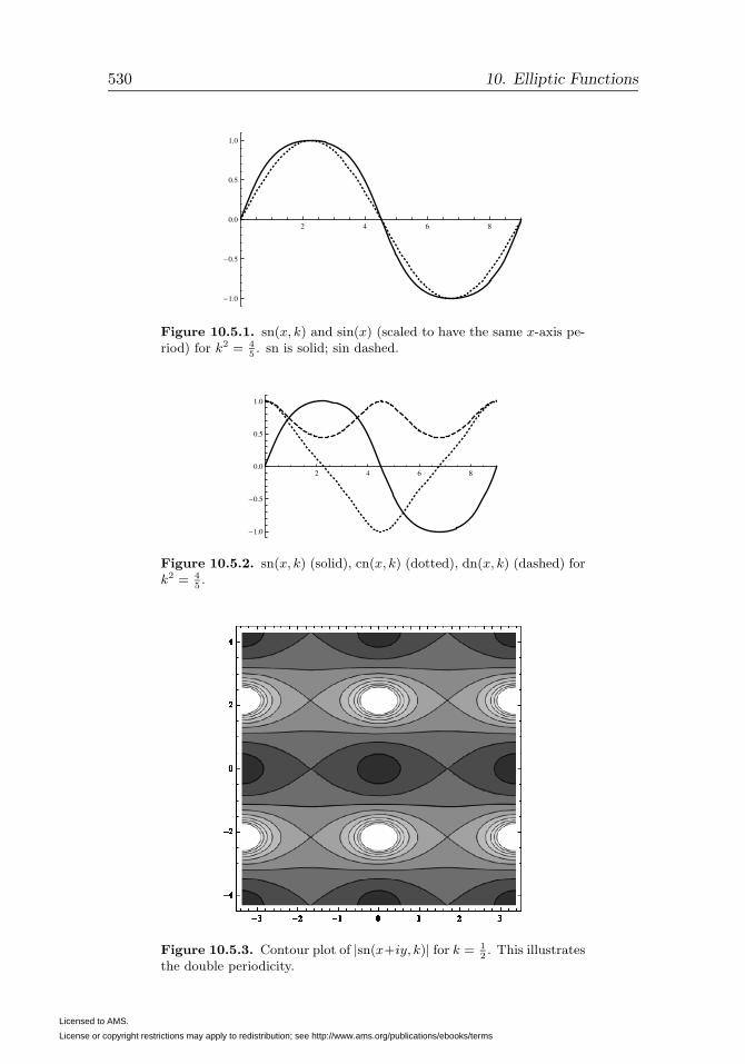
530 10. Elliptic Functions
2 4 6 8
−1.0
−0.5
0.0
0.5
1.0
Figure 10.5.1. sn(x, k) and sin(x) (scaled to have the same x-axis pe-riod) for k2 = 4
5. sn is solid; sin dashed.
2 4 6 8
−1.0
−0.5
0.0
0.5
1.0
Figure 10.5.2. sn(x, k) (solid), cn(x, k) (dotted), dn(x, k) (dashed) fork2 = 4
5.
Figure 10.5.3. Contour plot of |sn(x+iy, k)| for k = 12. This illustrates
the double periodicity.
Licensed to AMS.
License or copyright restrictions may apply to redistribution; see http://www.ams.org/publications/ebooks/terms

10.5. Jacobi Elliptic Functions 531
Theorem 10.5.6. Given k in (0, 1), let τ ∈ i(0,∞) be determined by
k2 =e2(τ)− e3(τ)
e1(τ)− e3(τ)(10.5.55)
where ej(τ) are the values of ℘(· | τ) on the half-lattice which obey e1 > e2 >e3. Let
μ =√e1 − e3 (10.5.56)
Then
sn(x, k) =μσ(x/μ)
σ3(x/μ)(10.5.57)
cn(x, k) =σ1(x/μ)
σ3(x/μ)(10.5.58)
dn(x, k) =σ2(x/μ)
σ3(x/μ)(10.5.59)
K =μ
2, K ′ = − iμτ
2(10.5.60)
Proof. We start with (10.4.69) by picking α0 =∞, and since ℘(u) = ℘(−u),flipping signs to get
u =
ˆ ∞
α
dy√4y3 − g2y − g3
⇔ ℘(u) = α (10.5.61)
In (10.5.1), we change variables to s2 = β, t2 = z to get (since dz = 2t dt =2√z dt)
x =
ˆ β
0
dz
2√z(1− z)(1− k2z)
⇔ β = sn(x)2 (10.5.62)
The square root in (10.5.61) has zeros at y = e1, e2, e3, while the onein (10.5.62), at z = 1, k−2, ∞. This suggests we pick a fractional lineartransformation that takes e1 to 1, e3 to ∞, and e2 to k−2, that is,
z =e1 − e3y − e3
(10.5.63)
does the right thing to e1 and e3. If we pick τ so that (10.5.55) holds, then(10.5.63) moves the zeros to the right place.
By (10.5.63) with μ given by (10.5.56),
y − e3 =μ2
z, y − e1 = μ2 (1− z)
z(10.5.64)
y − e2 = μ2 1− k2z
z, dz = − z2
μ2dy (10.5.65)
Licensed to AMS.
License or copyright restrictions may apply to redistribution; see http://www.ams.org/publications/ebooks/terms

532 10. Elliptic Functions
Thus, √4y3 − g2y − g3 = 2
√(y − e1)(y − e2)(y − e3)
=2μ3
z2
√z(1− z)(1− k2z)
(10.5.66)
sody√
4y3 − g2y − g3= − 1
μ
dz
2√
z(1− z)(1− k2z)(10.5.67)
Taking into account the change of variables in limits and the inversionof limits, (10.5.61), (10.5.62), and (10.5.67) translate to
α = ℘(u), β = sn(x)2 ⇔ u =x
μ, β =
μ2
α− e3(10.5.68)
or
sn(x) =μ√
℘(x/μ)− e3(10.5.69)
Given (10.4.86) for j = 3, this translates to (10.5.57). This plus (10.5.53)plus (10.4.86) for j = 1 and 3 implies (10.5.58), and similarly, (10.5.69) plus(10.5.54) plus (10.5.55) plus (10.4.86) for j = 2 and 3 implies (10.5.59).
K is determined by sn(K) = 1 which, given ℘(12) = e1 and (10.5.56),yields the first equation in (10.5.60).
Making the k- and τ -dependence explicit, we see if τ(k) solves (10.5.55),then
K(k) = 12
√e1(τ(k))− e3(τ(k)) (10.5.70)
If k2 obeys (10.5.55), then k′2 = (e2 − e1)/(e3 − e1). Thus τ(k′) obeys
e2(τ(k′))− e3(τ(k
′))
e1(τ(k′))− e3(τ(k′))=
e2(τ(k))− e1(τ(k))
e3(τ(k))− e1(τ(k))
Using e1 + e2 + e3 = 0, it is easy to see this is equivalent to
e1(τ(k′))
e3(τ(k′))=
e3(τ(k))
e1(τ(k))
Thus, we need to interchange the two lattice generators and replace one bythe negative. Using the invariance of ej/ek under scaling τ1 and τ2, thisimplies
τ(k′) = −τ(k)−1 (10.5.71)
Restoring the second element of the basis,
e1(−τ−1) = e1(1,−τ−1) = e3(τ−1, 1)
= τ2e3(1, τ) = τ2e3(τ) (10.5.72)
where we used the scale covariance (10.4.5) with λ = τ . There is a similarformula for e3.
Licensed to AMS.
License or copyright restrictions may apply to redistribution; see http://www.ams.org/publications/ebooks/terms

10.5. Jacobi Elliptic Functions 533
0.0 0.2 0.4 0.6 0.8 1.0
2.0
2.5
3.0
3.5
4.0
4.5
5.0
Figure 10.5.4. K(k) : 0 < k < 1.
Thus, (10.5.11) and (10.5.71) imply
K ′ = K(k′) = 12
√e1(−τ−1(k))− e3(−τ−1(k))
= 12
√τ2(e3(τ)− e1(τ))
= −iτK(k) (10.5.73)
verifying the second half of (10.5.60). Since τ ∈ C+ with Re τ = 0 ande3 < e1, the argument of the final square root is positive. We take −i in(10.5.73) to arrange that K ′ > 0. �
Figure 10.5.4 shows K(k) for 0 < k < 1. Note that limk↓0K(k) = π/2and there is a logarithmic divergence at k = 1.
Notes and Historical Remarks. Bernoulli [43] considered the sums∑∞n=0 x
n2and
∑∞n=0 x
n(n+1) and Euler [178] has several results on suchsums (and even a variant of triple product identity) and considered the θ-like product
∏∞n=1(1−xnz)−1. Gauss’ unpublished works on the lemniscate
integral contain objects we would now recognize as θ functions, both asproducts and sums. He found this in part by looking at the arithmetic-geometric mean (start with a0, b0, form an+1, bn+1 inductively by an+1 =12(an + bn), bn+1 =
√anbn; they have a common limit called the arithmetic
geometric mean), which he related to the lemniscate integral and wrote interms of theta functions. Cox [125] discusses both this mean and the history.
It was Jacobi, though, who first fully presented θ functions in his funda-mental work in 1829 on elliptic functions [281]. The four-fold θj is from his1835 paper [283]. For more on the history, see Hellegouarch [250, Ch. 5].For a recent book on theta functions, see Farkas–Kra [187].
As we have seen, Θ and θ obey a variety of remarkable relations. AsHellegouarch [250] remarks:
The originator of the famous wisecrack about the five operations
in arithmetic—addition, subtraction, multiplication, division and
Licensed to AMS.
License or copyright restrictions may apply to redistribution; see http://www.ams.org/publications/ebooks/terms

534 10. Elliptic Functions
modular functions—would appear to have been the mathematician
M. Eichler. As we will see, the fifth and last “operations” are
actually functions, which have so incredibly many symmetries that
one may really wonder how they can possibly exist.
Theta functions, as generalized by Riemann [484] to higher dimensions((10.5.20) is replaced by Θ(�z) =
∑n∈Zν exp(−(�n,A�n))zn1
1 . . . znνν for a suit-
able positive define matrix A) are the basis for the study of meromorphicfunctions on higher-genus Riemann surfaces and have many other applica-tions. See [274, 446, 472] and Section 11.6.
The reader should be warned that while our definitions of θj are verycommon, there are many, many other normalizations of functions called“theta”—as remarked in the Wikipedia article2 on “Jacobi theta-functions(notational variations)” (yes, there is an entire article on that subject!):“The warning in Abramowitz and Stegun, ‘There is a bewildering varietyof notations . . . in consulting books caution should be exercised,’ may beviewed as an understatement.”
The triple product formula appeared in Jacobi’s 1829 book [281] andit is often called the Jacobi triple product theorem, but there are the usualsuspects on the prehistory. Gauss also knew it and a special case appearedin Euler. [15] point out that it follows from what they call the q-binomialtheorem found by Rothe in 1811 [492] (see Problem 6). They also interpretthe triple product formula as an Euler duplication formula for q-Gammafunctions.
Carl Gustav Jacob Jacobi (1804–51) was, like Landau later, the son of aJewish banker based in Berlin, although, unlike Landau, he had to convertto Christianity to be eligible for academic appointment, and due to economicturmoil in Germany, he lost his family inheritance. In his later years, unableto teach because of ill health (diabetes), he depended on a royal stipend. In1851, at age only 47, he suffered first from influenza and then smallpox andpassed away.
He is best known for his work on elliptic functions, but also for continuedfractions (and the related Jacobi matrices), determinant theory (Jacobians),mechanics (Hamilton–Jacobi equations), number theory (much of it basedon his work on elliptic functions), special functions (Jacobi polynomials),and differential geometry (variational equations for geodesics).
The mention of q-binomial and q-Gamma function points out that θ func-tions are a part of what is sometimes called q-ology. While the formulae work
2http://en.wikipedia.org/wiki/Jacobi_theta_functions_(notational_variations)
Licensed to AMS.
License or copyright restrictions may apply to redistribution; see http://www.ams.org/publications/ebooks/terms

10.5. Jacobi Elliptic Functions 535
for q ∈ D, the intuition comes from q ∈ (0, 1). The q-integral is defined by
ˆ a
0f(x) dqx =
∞∑n=0
f(aqn)(aqn − aqn+1) (10.5.74)
the q-difference
(Δqf)(x) =f(x)− f(qx)
x− qx(10.5.75)
and the q-factorial and q-binomial coefficient
n!q =(1− q)(1− q2) . . . (1− qn)
(1− q)n(10.5.76)[
nk
]q
=n!q
k!q(n− k)!q(10.5.77)
The point is that one uses geometrically spaced values and defines objectsthat, as q → 1, approach their standard form (the reader should check thisfor the four q-objects just defined). Analogy to q = 1 gives one remark-able identities and relations. There are q-Gamma and q-beta functions,q-orthogonal polynomials, and a q-ology interpretation of the triple productformula. [15, Ch. 10] is a good introduction to q-ology.
As noted, there are many other evaluations of what we called Cq. SeeAndrews [13, 14] for two analytic calculations and Cheema [113], Wright[595], and [15, Ch. 11] for combinatorial proofs. Simon [524, Sec. 1.6] hasan interesting proof based on setting up a family of orthogonal polynomi-als on the unit circle (Rodgers–Szego polynomials) and analyzing them interms of q-binomial coefficients. Szego’s theorem for this set of polynomialsevaluates Cq.
For suitable values of parameters, θ obeys a heat equation. To get ridof annoying π’s, define
H(x, t) = θ3
(x
2π
∣∣∣∣ itπ)
=∞∑
n=−∞e−n2teinx (10.5.78)
and note that H obeys the heat equation for x = R, t > 0,
∂
∂tH(x, t) =
∂2
∂x2H(x, t) (10.5.79)
Indeed, it is the fundamental solution as periodic functions in x with H( · |t = 0) = cδ(x).
At first, some are puzzled about why there are four θ’s, four σ’s, andthree Jacobi elliptic. Why not just use a single function and ratios andtranslates? But, after all, we use not only sin but also cos and tan and . . . .In fact, there are standardly not three Jacobi functions but twelve! Going
Licensed to AMS.
License or copyright restrictions may apply to redistribution; see http://www.ams.org/publications/ebooks/terms

536 10. Elliptic Functions
back to Glaisher [209], they have easy-to-remember symbols, for example,cd(x) = cn(x)/dn(x). And they actually enter in integrals, for example,
x =
ˆ 1
cd(x)(1− t2)−1/2(1− k2t2)−1/2 dt
See Armitage–Eberlein [21, Ch. 2] for a summary. There are, of course,dozens of formulae for sums of arguments, algebraic relations, and integrals.The Problems have a selection of some of them.
Integrals of the form´ R(z)√
P (z)dz, where P is a polynomial of degree 3 or 4
and R is a rational function, are called elliptic integral. Legendre reducedsuch integrals to normal forms. As we did in the proof of Theorem 10.5.6for the special case (10.5.61), one can use fractional linear transformationsand quadratic change of variable to reduce to the special case P (z) = [(1−z2)(1− k2z2)]. By further use of integration by parts and that for this caseof P , if R(z) = zf(z2), we have a perfect derivative, Legendre reduced tothree normal forms:ˆ
dz√(1− z2)(1− k2z2)
,
ˆ √1− k2z2√1− z2
dz ,
ˆdz
(z2 − b)√
(1− z2)(1− k2z2)
(10.5.80)
called, respectively, elliptic integrals of the first kind, second kind, and thirdkind. Hancock [236, 237] from 1910 and 1917 are the standard “modern”references on elliptic integrals. Section 11.1 of Beals–Wong [32] has a text-book presentation of Legendre’s theorem that all elliptic integrals can bereduced to the three in (10.5.80).
Problems
1. (a) Prove that
σ(z) = eω1z2/2τ1 θ1(z)
θ′1(0)(10.5.81)
(b) Prove that for j = 1, 2, 3,
σj(z) = eω1z2/2τ1θj+1(z)
θj+1(0)(10.5.82)
2. One of the surprises in Theorem 10.5.3 is that one doesn’t assume a priorithat z = −q is the only zero in Aq,q−1 . This problem will take the mysteryout of that.
(a) If f obeys (10.5.14) and f(z) = g′(z)/g(z), prove that f(q2z) =f(z)− z−1.
Licensed to AMS.
License or copyright restrictions may apply to redistribution; see http://www.ams.org/publications/ebooks/terms

10.5. Jacobi Elliptic Functions 537
(b) Use the argument principle to show that if g obeys (10.5.14), then ghas exactly one zero in any Aq2a,a with g nonvanishing on ∂Dq2a.
3. Given the definitions of θj(z) in (10.5.36)–(10.5.39), prove that (10.5.41)–(10.5.43) are valid.
4. Given (10.5.57), prove that
sn(x+ 2K, k) = −sn(x, k), sn(x+ 2iK ′, k) = sn(x, k) (10.5.83)
What are the analogous periodicities of cn and dn?
5. Prove the q-binomial coefficients given by (10.5.77)/(10.5.76) obey[n+ 1k
]q
= qk[nk
]q
+
[n
k − 1
]q
=
[nk
]q
+ qn+1−k
[n
k − 1
]q
6. This problem will lead the reader through a proof of the q-binomial the-orem, that for |q| < 1, |z| < 1, and a ∈ C,
∞∑n=0
(a; q)n(q; q)n
zk =(az; q)∞(z; q)∞
(10.5.84)
where (including for n =∞)
(a; q)n =n∏
j=1
(1− aqj−1) (10.5.85)
(a) Let F (z) be the right-hand side of (10.5.84). Prove that F is analyticfor q, a fixed and z ∈ D. Write F (z) =
∑∞n=0 bnz
n.
(b) Prove that (1− z)F (z) = (1− az)F (qz).
(c) Prove that b1 = 1 and bn = [(1− aqn−1)/(1− qn)]bn−1 and concludethat bn = (a; q)n/(q; qn).
(d) Prove Rothe’s formula that
N∑k=0
[Nk
](−1)kqk(k−1)/2zk = (z; q)N (10.5.86)
(Hint: Take a = q−N .)
7. This will deduce the Jacobi triple product formula from Rothe’s formula.Take z ∈ C×.
(a) Prove that
(zq−n; q)2n = (−1)nznq−n2+n(n−1)/2(q/z; q)n(z; q)n (10.5.87)
Licensed to AMS.
License or copyright restrictions may apply to redistribution; see http://www.ams.org/publications/ebooks/terms

538 10. Elliptic Functions
(b) Take N = 2n in (10.5.86), replace z by zq−n, and use (10.5.87) toprove that
(q/z; q)n(z; q) =n∑
k=−n
(q; q)2n(−1)kqk(k−1)/2zk
(q; q)n+k(q; q)n−k
(c) Take n→∞ to obtain
(z; q)∞(q/z; q)∞(q; q)∞ =
∞∑k=−∞
(−1)kqk(k−1)/2zk (10.5.88)
(d) Replace q by q2 and z by −qz to get
(−qz; q2)∞(−q/z; q2)∞(q2; q2) =
∞∑n=−∞
qn2zn (10.5.89)
and verify that this is just the triple product formula (10.5.20).
8. For q ∈ D, prove that
(a)∞∑
n=−∞qn
2=
∞∏n=1
(1− q2n)(1 + q2n−1)2
(b)∞∑
n=−∞(−1)nqn2
=∞∏n=1
(1− q2n)(1− q2n−1)2
(c)∞∑
n=−∞(−1)nqn(3n+1)/2 =
∞∏n=1
(1− qn)
(d)∞∑n=0
qn(n+1)/2 =∞∏n=1
[1− q2n
1− q2n−1
](Hint: Use the triple product formula. For (c), replace q by q3/2 andz = −q1/2, and for (d), replace q by q1/2 and take z = q1/2.)
9. Let g(x) =´ x0 f(y) dqy and let Δq be given by (10.5.75). Prove that
(Δqg)(x) = f(x).
10. (a) Prove that for 0 < k < 1, ϕ ∈ (−π/2, π/2), we have, by a change ofvariables, that
ˆ ϕ
0
dψ√1− k2 sin2(ψ)
=
ˆ sin(ϕ)
0
dy√(1− k2y2)(1− y2)
This is another way that elliptic integrals and functions arise.
Licensed to AMS.
License or copyright restrictions may apply to redistribution; see http://www.ams.org/publications/ebooks/terms

10.5. Jacobi Elliptic Functions 539
(b) Prove that
K(k) =
ˆ π/2
0
dψ√1− k2 sin2(ψ)
(10.5.90)
(c) Fix k ∈ (0, 1). For x ∈ (−K,K), define ϕ(x) ∈ (−π/2, π/2) to be theunique solution of
x =
ˆ ϕ(x)
0
dψ√1− k2 sin2(ψ)
Prove that
sn(x, k) = sin(ϕ(x)), cn(x, k) = cos(ϕ(x)) (10.5.91)
(d) Prove that
dϕ
dx=
√1− k2 sin2(ϕ(x)) = dn(x, k) (10.5.92)
and from that, prove that
d
dxsn(x) = cn(x) dn(x) (10.5.93)
(e) Prove that d2ϕdx2 = −1
2k2 sin(2ϕ) so that η = 2ϕ for k suitable solves
the pendulum differential equation d2ηdx2 = −ω2 sin(η). (Hint: Apply d
dx to
(dϕdx )2 = 1− k2 sin2(ϕ).)
Remark. The function ϕ defined by sn(x, k) = sin(ϕ(x)) is sometimescalled the Jacobi amplitude function, written am(x, k) as in sn(x, k) =sin(am(x, k)).
11. (a) Using the product formula for Θ, prove that
Θ(1 | q)Θ(−1 | q) =∞∏n=1
(1− q2n)2(1− q4n−2)2 (10.5.94)
(b) Prove that
Θ(1 | q)Θ(−1 | q)Θ(q | q) = 2
∞∏n=1
(1− q2n)3 (10.5.95)
(c) Prove that
Θ′(−q | q) = q−1∞∏n=1
(1− q2n)3 (10.5.96)
(d) Define four constants that are in (10.5.81) and (10.5.82),
θj = θj(0), j = 2, 3, 4; θ′1 = θ′1(0) (10.5.97)
Licensed to AMS.
License or copyright restrictions may apply to redistribution; see http://www.ams.org/publications/ebooks/terms

540 10. Elliptic Functions
where θj is related to Θ by (10.5.36)–(10.5.39). Prove that
θ′1 = πθ2θ3θ4 (10.5.98)
12. This problem will establish the main formulae that write the Jacobi ellip-tic functions in terms of {θj(w)}4j=1 and the constants of (10.5.97). You
need Theorem 10.5.6, (10.5.81)/(10.5.82), and (10.5.98).
(a) Prove that √℘(z)− ej =
θ′1θj+1
θj+1(z)
θ1(z)
and conclude that √e1 − ej =
θ′1θj+1
θj+1(12)
θ1(12)
so that
√e1 − e2 =
θ′1θ4θ3θ2
= πθ24 and μ ≡√e1 − e3 = πθ23 (10.5.99)
(b) Similarly, prove that√e2 − e3 = πθ22 (10.5.100)
(c) Using (a) + (b), prove that
θ22 + θ24 = θ23 (10.5.101)
(d) Prove (10.5.101) using the product formulae.
(e) Prove that
k =θ22θ23
, k′ =θ24θ23
, K =π
2θ23 , K ′ = − iπτ
2θ23 (10.5.102)
(f) Prove that
sn(2Kw) =1√k
θ1(w)
θ4(w), cn(2Kw) =
√k′
k
θ2(w)
θ4(w),
dn(2Kw) =√k′
θ3(w)
θ4(w)
(10.5.103)
(g) Prove that
sn(K) = 1 (10.5.104)
13. This problem will verify the original relation that Legendre proved thatis equivalent to what we’ve called the Legendre relation (see (10.3.32)),
Licensed to AMS.
License or copyright restrictions may apply to redistribution; see http://www.ams.org/publications/ebooks/terms

10.5. Jacobi Elliptic Functions 541
although it looks quite different. The complete elliptic integrals of thesecond kind are
E(k) =
ˆ π/2
0
√1− k2 sin2(ψ) dψ =
ˆ 1
0
√1− k2t2
1− t2dt (10.5.105)
If E = E(k) and E′ = E(k′), then the Legendre relations that you’llprove say that
EK ′ + E′K −KK ′ =π
2(10.5.106)
(a) Prove that
E =
ˆ K
0(dn)2(x) dx (10.5.107)
(Hint: Use (10.5.91), (10.5.92), and (10.5.104).)
(b) Prove that
E = μ
ˆ 1/2
01 +
(e3 − e2
℘(y)− e3
)dy (10.5.108)
(Hint: Use (10.5.59) and (10.4.84).)
(c) Prove that
E =μ
2− 1
μ
ˆ 1/2
0(℘(y + τ)− e3) dy (10.5.109)
(Hint: Use Problem 6 of Section 10.4.)
(d) Prove that (ω1 is given in (10.4.13))
E =e1 + ω1
μ(10.5.110)
(Hint: Use (10.4.25) and (10.4.28).)
(e) Similarly, prove that
E′ =i(τe3 + ω3)
μ(10.5.111)
(f) Prove the Legendre relation (10.5.106). (Hint: Use (10.5.60) and(10.3.32).)
14. With K given by (10.5.50), E by (10.5.105), and k′ by (10.5.49), provethat
dE
dk(k) =
E(k)−K(k)
k,
dK
dk(k) =
E(k)− (k′)2K(k)
k(k′)2(10.5.112)
Licensed to AMS.
License or copyright restrictions may apply to redistribution; see http://www.ams.org/publications/ebooks/terms

542 10. Elliptic Functions
15. Let 0 < k < 1. This problem will prove for x real,∣∣∣∣sn(x+iK ′
2
)∣∣∣∣ = k−1/2 (10.5.113)
a fact used in Examples 8.4.5 and 8.4.14.
(a) Using (10.5.60) and (10.5.69), prove that
sn(K) = 1, sn(K + iK ′) = k−1 (10.5.114)
(b) Using (10.5.60) and (10.5.69), prove that sn(z + iK ′) and sn(z) havezeros and poles reversed and conclude that
sn(z)sn(z + iK ′) = k−1 (10.5.115)
(Hint: First prove the product is constant and then evaluate it at z = K.)
(c) Prove (10.5.113). (Hint: sn is real on R so sn(z) = sn(z).)
Note. See Problem 7 of Section 10.4 for a related result.
10.6. The Elliptic Modular Function
This section will study the function
λ(τ) =e2(τ)− e3(τ)
e1(τ)− e3(τ)(10.6.1)
called the elliptic modular function. From the point of view of this chapter,this will allow the solution of elliptic integral inversion problems, specificallythe questions of what values of k2 in (10.5.1) can occur and what g2, g3 in(10.4.81) can occur as we vary τ or τ1, τ2. From this standpoint, the mainresults of this section are:
(1) λ is a bijection of {iy | 0 < y < ∞} ≡ K and (0, 1), and for τ ∈K, e1(τ) > e2(τ) > e3(τ). This was used in the last section and, inparticular, says that all classical elliptic integrals of the form (10.5.1)fall within the purview of Theorem 10.5.6.
(2) λ maps C+ to C\{0, 1}, is locally one-one, and its restriction to F , thefundamental domain for Γ(2), is a bijection to C \ {0, 1}. (Note thatthis bijection is continuous, but its inverse is not in the topology as asubset of C; if we think of F ∼= C \ Γ(2) with the quotient topology, itis.) Thus, the extension of Theorem 10.5.6 to complex k2 handles allcases k2 �= 0, 1. Of course, the elliptic integrals for k = 0, 1 are triviallydoable without recourse to elliptic functions (k = 0 is arcsin and k = 1is arctanh).
(3) For every g2, g3, with Δ �= 0, there is a τ1, τ2 in C××C×, with τ2/τ1 /∈ R,so that g2(τ1, τ2) = g2, g3(τ1, τ2) = g3 (again, if Δ = 0, the integral isdoable in terms of inverse trigonometric functions). The map τ → J(τ)
Licensed to AMS.
License or copyright restrictions may apply to redistribution; see http://www.ams.org/publications/ebooks/terms

10.6. The Elliptic Modular Function 543
is a bijection of F and C, although not a local bijection at some pointsin ∂F , that is, J : C+ → C is not everywhere a local bijection.
From a perspective that goes beyond elliptic functions:
(1) τ → λ(τ)− i
λ(τ) + i(10.6.2)
is a Riemann map of {τ | 0 < Re τ < 1; |τ − 12 | >
12} to D, so an interesting
example in an atlas of conformal maps. See Example 8.4.9.
(2) λ : C+ → C \ {0, 1} is onto, a local bijection, and λ(z) = w if and onlyif there exists γ ∈ Γ(2) so that z = γ(w). This will implement thefunction needed for the proofs of Picard’s theorems (see Section 10.3).It is the third construction of this map (see Sections 8.3 and 8.5).
Recall what we learned in Problem 8 of Section 10.4:
λ(τ) = 16eiπτ +O(e−3|Im τ |) (10.6.3)
as Im τ → ∞ with Re τ ∈ [0, 2] (we’ll see shortly, uniformly in all real τ)and, in particular,
λ(τ)→ 0 as Im τ →∞ (10.6.4)
Moreover, again by Problem 8 of Section 10.4, for Im τ large, once we knowej(τ) are real on i(0,∞), we have
e1 > e2 > e3 (10.6.5)
and by continuity and (10.6.7) below, this holds for all τ ∈ i(0,∞); see alsoProblem 13 of Section 10.4.
Finally, since ℘(z) − ej has only one (double) zero in the fundamentalcell,
e1 �= e2 �= e3 �= e1 (10.6.6)
We begin this section’s analysis with the covariance properties of λ underthe action of SL(2,Z).
Theorem 10.6.1. (a) If ( a bc d ) ∈ Γ(2), then
λ
(aτ + b
cτ + d
)= λ(τ) (10.6.7)
(b) λ
(−1
τ
)= 1− λ(τ) (10.6.8)
(c) λ(τ + 1) = −λ(τ)(1− λ(τ))−1 (10.6.9)
Proof. (a) If τ1 = d+ cτ , τ2 = b+ aτ , then τ = (aτ + b)/(cτ + d) = τ2/τ1is the τ for the new lattice. Not only does this preserve L1,τ , and so ℘(z),but if a, d are odd and b, c even, ℘(τ1/2) = ℘(12), ℘(τ1/2) = ℘(τ/2) since
τ1/2− 12 , τ2/2− τ/2 ∈ L1,τ . Thus, ej(τ1, τ2) = ej(1, τ) and λ is unchanged.
Licensed to AMS.
License or copyright restrictions may apply to redistribution; see http://www.ams.org/publications/ebooks/terms

544 10. Elliptic Functions
(b) If τ1 = τ , τ2 = −1, then τ = −1/τ and e2 is unchanged (since 12(τ1 +
τ2)− 12(1 + τ) = −1 ∈ L1,τ ), but e1 and e3 are interchanged. Thus,
λ
(−1
τ
)=
e2(τ)− e1(τ)
e3(τ)− e1(τ)= 1− λ(τ)
(c) Similarly, τ1 = 1, τ2 = 1 + τ has τ = 1 + τ and e1 is unchanged, but e2and e3 are interchanged. Thus,
λ(1 + τ) =e3 − e2e1 − e2
= − λ
1− λ�
We said the action of all of SL(2,Z), but SL(2,Z)/Γ(2), has six elementsnot two. However, using cycle notation (see the Notes), the two permuta-tions we look at, namely, (13) and (23), generate the whole group, so the fullaction is easy to obtain, summarized in the following table (see Problem 1):
� (123) (132) (12) (13) (23)
τ τ −1/(τ + 1) −1− 1/τ τ/(1 + τ) −1/τ τ + 1
λ(τ) λ (1− λ)−1 1− λ−1 λ−1 1− λ −λ(1− λ)−1
Theorem 10.6.2. (a) λ is real if τ is contained in ∂F � ≡ {τ | Re τ = 0 orRe τ = 1 or |τ − 1
2 | =12} ∩ C+.
(b) λ→ 0 uniformly in Re τ as Im τ →∞.(c) λ → 1 (respectively, ∞) as τ → 0 (respectively, 1) in C+ with arg(τ)
(respectively, arg(τ − 1)) in (ε, π − ε) for any ε > 0.(d) For all τ ∈ C+, λ(τ) is never 0, 1, or ∞.(e) λ[{iy | y ∈ (0,∞)}] = (0, 1), λ[{12 + 1
2eiθ | θ ∈ (0, π)}] = (1,∞),
λ[{1 + iy | y ∈ (0,∞)}] = (−∞, 0).
Remarks. 1. We’ll see shortly that λ takes every value in C \ {0, 1} andthat λ is one-one on each of the sets in (v).
2. As our proof shows, λ(τ) → 1 as Im(−1/τ) → ∞. This is not thesame as |τ | → 0, Im τ > 0. For example, if τ = ε + iε2, then Im(1/τ) =ε2/(ε2 + ε4)→ 1 as ε ↓ 0.
Proof. (a) Suppose first Re τ = 0, so τ = iy and Lτ = {n1 + in2y}. SinceLτ = Lτ , the formula (10.4.29) for ℘ proves that
℘(z | 1 iy) = ℘(z | 1 iy) (10.6.10)
Licensed to AMS.
License or copyright restrictions may apply to redistribution; see http://www.ams.org/publications/ebooks/terms

10.6. The Elliptic Modular Function 545
Since always ℘(−z | 1 τ) = ℘(z | 1 τ), we have
℘(−z | 1 iy) = ℘(z | 1 iy)
Thus, e1 and e3 are real, and since e1 + e2 + e3 = 0, e2 is also real, so λ isreal. By (10.6.9), λ is real on Re τ = 1, and similarly, λ is real if Re τ = −1.τ → −1/τ maps −1 to 1 and ∞ to 0 and maps R to R, {τ | Re τ = −1}is mapped to a circle orthogonal to R, so the circle |τ − 1
2 | =12 (as algebra
also shows) and C+ ∩ {τ | Re τ = −1} is mapped to C+ ∩ {τ | |τ − 12 | =
12}.
Thus, by (10.6.8), λ is real on C+ ∩ {τ | |τ − 12 | =
12}.
(b) Since ( 1 20 1 ) ∈ Γ(2), λ(τ+2) = λ(τ), so (10.6.3) uniformly for Re τ ∈ [0, 2]
implies it for all Re τ .
(c) By (10.6.8), λ → 1 as Im(−1/τ) → ∞, and with the restriction onarg(τ), |τ | → 0 ⇒ Im(−1/τ) → ∞. Then, by (10.6.9), we get from τ → 0to τ → 1.
(d) This is immediate from e1 �= e2 �= e3 �= e1.
(e) Since λ is real, never 1 or 0, and λ(iy) → 1 as y → ∞ and λ(iy) → 1as y → 0, it must take all values and only those values on {iy | y ∈ (0,∞)}.(10.6.9) and λ(τ − 2) = λ(τ) imply λ takes all values in (−∞, 0) on ±1+ iyand thus, (10.6.8) yields the result on {z | |z − 1
2 | =12} ∩ C+. �
Here is (part (a) below) the most subtle argument in the analysis ofλ(τ). Let
F � = {τ | Im τ > 0, 0 < Re τ < 1, |τ − 12 | >
12} (10.6.11)
Theorem 10.6.3. (a) λ is a bijection of F � to C+.(b) λ is a bijection of F to C \ {0, 1}.(c) λ′(z) �= 0 for all z in C+.(d) λ(z) = λ(w)⇔ z = (aw + b)/(cw + d) for some ( a b
c d ) ∈ Γ(2).
Proof. (a) Fix ε and let Γε be the following contour in F � (Figure 10.6.1).
Γ1 Γ5
Γ6
Γ3
Γ2 Γ4
Figure 10.6.1. Contour around ˜F cutoff.
Licensed to AMS.
License or copyright restrictions may apply to redistribution; see http://www.ams.org/publications/ebooks/terms

546 10. Elliptic Functions
λ[Γ ]4
λ[Γ ]1
λ[Γ ]2
λ[Γ ]3λ[Γ ]5
λ[Γ ]6
0 1
Figure 10.6.2. Image of Γ under the elliptic modular function.
Start at iε−1 and go down to iε (call this Γ1), then go along the curveΓ2(x) = (x−iε−1)−1 = (x+iε−1)/(ε−2+x2), 0 ≤ x ≤ 1, from iε to the circle|τ − 1
2 | =12 (⇔ Re( 1τ = 1) (call this Γ2), then along this circle to the circle
reflection of Γ2 (call this Γ3), then around that curve Γ4(x) = 1−Γ2(1− x)near Re τ = 1 (call this Γ4). Γ4 is the reflection of Γ2 in the line Re τ = 1
2 .
Then up to 1+ iε−1 (call this Γ5), and across to iε−1 along Im τ = ε−1 (callthis Γ6).
The image, λ[Γ], (Figure 10.6.2), also has six pieces. λ[Γ1] runs fromnear 0 to near 1 along R. It can, a priori, wander back and forth, butstays on R. λ[Γ2] stays in a tiny neighborhood of w = 1. λ[Γ3] and λ[Γ5]stay along R, running from just above 1 to near ∞ and from above −∞ tobelow 0, and λ[Γ6] near λ = 0.
The key piece is λ[Γ4]. Γ2(x) is picked so Γ2(x)−1 = x − iε−1. By
(10.6.3),
λ(Γ2(x)−1) = 16e−ε−1
eiπx +O(e−3ε−1)
so, by (10.6.8), we have
λ(Γ2(x)) = 1− 16e−ε−1e−iπx +O(e−3ε−1
)
Note that since λ is real on Re τ = 0, λ(−τ) = λ(τ). Since Γ4(x) =
1− Γ2(1− x), by (10.6.9),
λ(Γ4(x)) = (16)−1eε−1eiπx + (1 +O(e−2ε−1
)) (10.6.12)
Then λ(Γ) goes along R with two tiny approximate half-loops near 0 and 1,and a huge semicircle looping back in the upper half-plane near infinity.
If η ∈ C+ and |η| is much smaller than O(eε−1) and farther from 0 and 1
than O(e−ε−1), then λ(Γ) will have winding number 1 about η and 0 about η.
By the argument principle, this implies (a).
(b), (c) Since λ is real on Re z = 0,
λ(−τ) = λ(τ) (10.6.13)
so λ is one-one on −F �, and since that set is open, λ′ �= 0 there. This set,
together with F �, covers all of F , except for the edges and for Re τ = 0.
Licensed to AMS.
License or copyright restrictions may apply to redistribution; see http://www.ams.org/publications/ebooks/terms

10.6. The Elliptic Modular Function 547
−2 −1 1 2
−1.0
−0.8
−0.6
−0.4
−0.2
0.2
0.4
Figure 10.6.3. Reλ(x+ i), −2 < x < 2.
Figure 10.6.4. Re and Im of λ(x+ iy), −3 < x < 3, 0 < y < 2.
λ is real on Re τ = 0 with values in (0, 1), Since Im τ > 0 on 0 < Re τ < εand Im τ < 0 on −ε < Re τ < 0, λ′ �= 0 on Re τ = 0 (see Problem 2). Sincedλ(iy)dy is real and nonvanishing, it has a single sign which, given the limiting
values, must be negative. So λ is one-one on Re τ = 0. By the covariance inTheorem 10.6.1, λ �= 0 and λ is one-one on {τ | Im τ > 0, Re τ = 1} and on
{τ | Im τ > 0, |τ − 12 | =
12}. This plus (a) proves that λ is a bijection of F
and C×. By invariance under Γ(2), we get λ′ �= 0 on all of C+.
(d) Theorem 10.6.1 implies w = γ(z)⇒ λ(w) = λ(z). On the other hand, if
w, z ∈ C+ with λ(w) = λ(z), there exists γ, γ ∈ Γ(2) so γ(w), γ(z) ∈ F and,
by invariance of λ, λ(γ(w)) = λ(γ(z)). Since λ is one-one on F , γ(w) = γ(z),so w = γ−1γ(z). �
Figure 10.6.3 plots Reλ(x + i) and Figure 10.6.4 has contour plots ofReλ(x+ iy) and Imλ(x+ iy).
We can immediately obtain the first two and the fourth and fifth resultsadvertised at the start of this section.
Theorem 10.6.4. The map of (10.6.2) is the unique map of F � to D withlimiting values −1 at τ =∞, (1− i)/(1 + i) at τ = 0 and +1 at τ = 1.
Theorem 10.6.5. λ : C+ → C\{0, 1} is a local bijection onto all of C\{0, 1}and λ(z) = w ⇔ ∃γ ∈ Γ(2), z = γ(w).
Theorem 10.6.6. For τ ∈ {iy | y ∈ (0,∞)}, e1 > e2 > e3, and for anyk2 ∈ (0, 1), there is a unique y ∈ (0,∞), so λ(iy) = k2.
Licensed to AMS.
License or copyright restrictions may apply to redistribution; see http://www.ams.org/publications/ebooks/terms
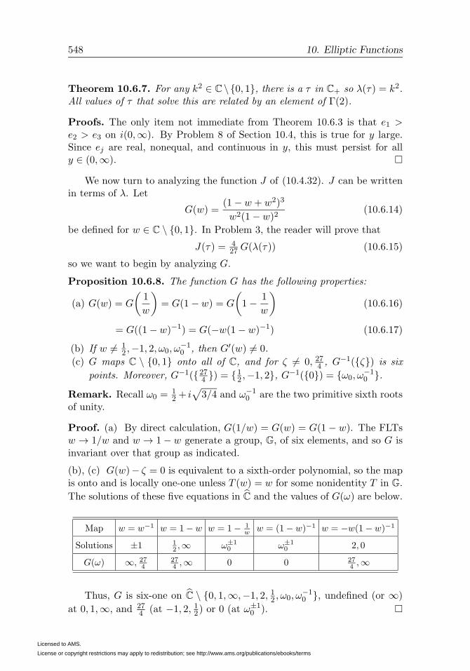
548 10. Elliptic Functions
Theorem 10.6.7. For any k2 ∈ C\{0, 1}, there is a τ in C+ so λ(τ) = k2.All values of τ that solve this are related by an element of Γ(2).
Proofs. The only item not immediate from Theorem 10.6.3 is that e1 >e2 > e3 on i(0,∞). By Problem 8 of Section 10.4, this is true for y large.Since ej are real, nonequal, and continuous in y, this must persist for ally ∈ (0,∞). �
We now turn to analyzing the function J of (10.4.32). J can be writtenin terms of λ. Let
G(w) =(1− w + w2)3
w2(1− w)2(10.6.14)
be defined for w ∈ C \ {0, 1}. In Problem 3, the reader will prove that
J(τ) = 427 G(λ(τ)) (10.6.15)
so we want to begin by analyzing G.
Proposition 10.6.8. The function G has the following properties:
(a) G(w) = G
(1
w
)= G(1− w) = G
(1− 1
w
)(10.6.16)
= G((1− w)−1) = G(−w(1− w)−1) (10.6.17)
(b) If w �= 12 ,−1, 2, ω0, ω
−10 , then G′(w) �= 0.
(c) G maps C \ {0, 1} onto all of C, and for ζ �= 0, 274 , G−1({ζ}) is six
points. Moreover, G−1({274 }) = {12 ,−1, 2}, G−1({0}) = {ω0, ω
−10 }.
Remark. Recall ω0 =12 + i
√3/4 and ω−1
0 are the two primitive sixth rootsof unity.
Proof. (a) By direct calculation, G(1/w) = G(w) = G(1− w). The FLTsw → 1/w and w → 1− w generate a group, G, of six elements, and so G isinvariant over that group as indicated.
(b), (c) G(w)− ζ = 0 is equivalent to a sixth-order polynomial, so the mapis onto and is locally one-one unless T (w) = w for some nonidentity T in G.
The solutions of these five equations in C and the values of G(ω) are below.
Map w = w−1 w = 1− w w = 1− 1w w = (1− w)−1 w = −w(1− w)−1
Solutions ±1 12 ,∞ ω±1
0 ω±10 2, 0
G(ω) ∞, 274
274 ,∞ 0 0 27
4 ,∞
Thus, G is six-one on C \ {0, 1,∞,−1, 2, 12 , ω0, ω−10 }, undefined (or ∞)
at 0, 1,∞, and 274 (at −1, 2, 12) or 0 (at ω±1
0 ). �
Licensed to AMS.
License or copyright restrictions may apply to redistribution; see http://www.ams.org/publications/ebooks/terms

10.6. The Elliptic Modular Function 549
Figure 10.6.5. Im J [x + iy] for −1 < x < 1, 0 < y < 2 and a blowupof a small piece.
Theorem 10.6.9. J (defined on C+ by (10.4.32)) has the following prop-erties:
(a) J is invariant under the action of SL(2,C) and J(τ) = J(τ) if and onlyif there is A ∈ SL(2,C) so τ = gA(τ).
(b) J maps C+ to all of C.(c) J ′(z) = 0 only if z = i or ω0 or an image under the action of SL(2,C).
J(i) = 1, J(ω0) = 0.
J(τ) has a third-order zero at ω0 and J(τ) − 1 has a second-order zero atτ = i.
Remarks. 1. The degeneracies and orders can be interpreted in terms ofthe sixth-order rotation symmetry of J1,ω0 and the fourth-order rotationsymmetry of J1,i.
2. Figure 10.6.5 shows ImJ(x+ iy) for −1 < x < 1, 0 < y < 2 and a blowupof the region near x = 0.3 + i0. Note that J is real on ∂F and its images,so these curves are contours in the contour plot of Im J .
Proof. (a) Since λ is invariant under Γ(2), by (10.6.15), J is invariantunder Γ(2). By Theorem 10.6.1 and Proposition 10.6.8, J(−1/τ) = J(τ)and J(τ + 1) = J(τ). Since SL(2,Z) is generated by Γ(2) (see Problem 4),±( 0 1
−1 0 ) and ±( 1 11 0 ), we have invariance under SL(2,Z).
Given that λ is one-one on F and the six-one nature of G and six-foldintersection of SL(2,Z) orbits with F , we see that J is one-one on F . Thisimplies J(τ) = J(τ) if and only if τ is on the orbit of τ .
(b) This follows from the fact that λ is onto C \ {0, 1} and that G mapsC \ {0, 1} to all of C.
(c) By (10.6.15),
J ′(τ) = 427 G
′(λ(τ))λ′(τ) (10.6.18)
Licensed to AMS.
License or copyright restrictions may apply to redistribution; see http://www.ams.org/publications/ebooks/terms

550 10. Elliptic Functions
and λ′ is nonvanishing, J ′(τ) = 0 ⇔ G′(λ(τ)) = 0. By Proposition 10.6.8,this happens if λ(τ) ∈ {12 ,−1, 2, ω0, ω
−10 }. Because of the invariance of G
in (10.6.16), this is orbits under SL(2,C) of any points where λ(τ) = 12 or
λ(τ) = ω0. By Problem 5, λ(i) = 12 and λ(ω0) = ω0, and so λ is one-one
on F . These are the only Γ(2) orbits where λ(τ) is 12 or ω0. The calculation
of the orders of the zeros of J ′ is left to Problem 6. �
Theorem 10.6.10. For any g2, g3 in C2 with g32 − 27g23 �= 0, there ex-ists τ1, τ2 in C2 with Im(τ2/τ1) > 0 so that (℘(z | τ1τ2), ℘′(z | τ1τ2)) obey(10.4.40).
Proof. Suppose first that g3 �= 0. Then g32/(g32 − 27g23) �= 1 so, by The-
orem 10.6.9, there is τ solving J(τ) = g32/(g32 − 27g23) and g1(1, τ) �= 0,
since J(τ) �= 1. Picking τ1 = μ, τ2 = μτ , we can arrange g3 = g3. SinceJ(τ) = J(τ), we see g32 = g32, so g2 = ωg2 for ω a cube root of unity. Sinceg2(μτ1, μτ2) = μ−4g2,
g3(μτ1, μτ2) = μ−6g3 (10.6.19)
we pick μ = ω−1. Then g2(μτ1, μτ2) = μ−4g2 = ωg2 = g2 and g3(μτ1, μτ2) =μ−6g3 = g3 = g3,
If g3 = 0, take τ1 = μ, τ2 = iμ so, by (10.6.19), g3(μ, iμ) =−g3(iμ,−μ) = −g3(μ, iμ) since S2k(τ1, τ2) = S2k(±τ1,±τ2) = S2k(τ2, τ1).Thus, g3(μ, iμ) = 0 and g2 �= 0. On the other hand, S4(1, i) �= 0 and thuswe can pick μ = (g1(1, i)/g2)
1/4 to get the desired value for g2. �
Notes and Historical Remarks. The term modular function is some-times applied to any meromorphic function on C+ invariant under the ac-tion of the modular group SL(2,C) or a large subgroup like Γ(2) and which
obeys |f(τ)| ≤ Ce−K|Im τ | if Im τ > T for some C,K, T . λ is then calledthe λ-invariant or λ-modular function and J , the j-invariant or Klein’s J in-variant, after work of Klein [309, 310]. A modular form of weight k hasf((aτ + b)/(cτ + d)) = (cτ + d)kf(τ) for some k. There are many books onmodular forms [140, 257, 322, 386], most on their connections to numbertheory; see Section 13.1 of Part 2B.
Jacobi proved a remarkable explicit formula for Δ(τ) in terms of q =e2πiτ (q = q2 for our usual q), namely,
Δ(τ) = (2π)12q∏n≥1
(1− qn)24
See Apostol [18], Serre [518], and Silverman [521] for proofs.
It turns out j(τ) = 1728J(τ) has remarkable properties. 1728 = 123 ispicked in part to make the leading coefficient in the series in e2πiτ (leadingas τ → i∞) 1, but makes all the other Fourier coefficients integral and
Licensed to AMS.
License or copyright restrictions may apply to redistribution; see http://www.ams.org/publications/ebooks/terms

10.6. The Elliptic Modular Function 551
many other objects integral and is of number-theoretic and group-theoreticsignificance.
(i1 . . . i�), with all ij distinct, is shorthand for the permutation that takesi1 → i2, i2 → i3, . . . , i� → i1 and leaves all other indices fixed.
Problems
1. Verify the table before Theorem 10.6.2 of maps τ → τ that implementthe permutations on ej(τ) (up to overall scaling) and the induced mapson λ.
2. If f is analytic in Dε(0) with ± Im f(z) ≥ 0 if ± Im z > 0, prove thatf ′(z) �= 0 in (−ε, ε).
3. (a) Prove that (with λ = (e2−e3)/(e1−e3)) that (1+λ+λ2)(e1−e3)2 =
34g2.
(b) Using (10.4.74), verify that [λ(1− λ)(e1 − e3)3]2 = Δ/16.
(c) With g given by (10.6.14) and J(τ) by (10.4.77), prove that (10.6.15)holds.
4. Prove that SL(2,Z) is generated by Γ(2) ∪ {±( 0 1−1 0 ),±( 1 1
1 0 )}.
5. (a) If τ = i, prove that ℘(iz | i) = −℘(z | i) and that e3 = −e1, e2 = 0,and then that λ(i) = 1
2 .
(b) If τ = ω0, prove that ℘(ω0z | ω0) = ω−20 ℘(z | ω0) and that e3 = ω−2
0 e1,
e2 = ω−40 e1, and λ(ω0) = ω0.
6. (a) Prove that near τ = i, J is two-one so that J ′(i) = 0, J ′′(i) �= 0.
(b) Prove that, near τ = ω0, J is three-one so that J ′(ω0) = J ′′(ω0) = 0,J ′′′(ω0) �= 0.
7. (a) Let f(τ), defined and analytic for τ ∈ C+, obey f(τ + �) = f(τ) for
some integral �. Prove that there exists K > 0 so |f(τ)| ≤ CeK|Im τ | ifand only if f has a convergent expansion (uniformly on compact subsetsof C+)
f(τ) =∞∑
n=−m
ane2πinτ/�
for m <∞.
(b) A modular function is a function meromorphic on C+, invariant under
SL(2,Z), with |f(τ)| ≤ CeK|Im τ | for some K <∞ and all τ with |Im τ | >T for some T . Prove that every rational function of J(τ) is a modularfunction and vice-versa.
Licensed to AMS.
License or copyright restrictions may apply to redistribution; see http://www.ams.org/publications/ebooks/terms

552 10. Elliptic Functions
8. A modular form of weight k is like a modular function except invarianceunder SL(2,Z) is replaced by f((aτ+b)/(cτ+d)) = (cτ+d)kf(τ). Provethat S2�(1, τ) is a modular form of weight 2�.
10.7. The Equivalence Problem for Complex Tori
In Section 7.1, we induced complex tori, Jτ1,τ2 for Im(τ2/τ1) > 0. In thissection, we’ll provide necessary and sufficient conditions for Jτ1,τ2 and Jτ1,τ2
to be conformally equivalent and, coincidentally, do the same for classifyingcubic curves. Here are the main theorems:
Theorem 10.7.1. Let τ1, τ2, τ1, τ2, all in C×, be such that τ ≡ τ2/τ1, τ ≡τ2/τ1 are both in C+. Then the following are equivalent:
(1) Jτ1,τ2 and Jτ1,τ2 are conformally equivalent.(2) For some λ ∈ C×, Lτ1,τ2 = λLτ1,τ2.(3) For some A ∈ SL(2,Z), τ = gA(τ).(4) J(τ) = J(τ) (10.7.1)
Theorem 10.7.2. The elliptic curves generated by y2 = 4(x3 − g2x − g3and y2 = 4x3 − g2x− g3 (where g32 − 27g23 �= 0 �= g32 − 27g23) are conformallyequivalent if and only if
g32g32 − 27g23
=g32
g32 − 27g23(10.7.2)
Proof of (2) ⇔ (3) ⇔ (4) ⇒ (1) in Theorem 10.7.1. If the latticesare the same, then there is ( a b
c d ) ∈ SL(2,C) so
τ1 = aλτ1 + bλτ2 (10.7.3)
τ2 = cλτ1 + dλτ2 (10.7.4)
Thus, τ = gA(τ). Conversely, if τ = gA(τ), we can pick λ so (10.7.3) holds,and then (10.7.4) will hold, and so Lτ1,τ2 = λLτ1,τ2 .
(3)⇔ (4) is immediate from Theorem 10.6.9. If (2) holds, f([z]) = [λ−1z]defines an analytic bijection of C/Lτ1,τ2 to C/Lτ1,τ2 . �
We’ll first provide two proofs of (1) ⇒ (2): one using uniqueness ofuniversal covering spaces and the other, the elliptic modular function.
First proof of (1) ⇒ (2) in Theorem 10.7.1. Let π : C → Jτ1,τ2 andπ : C → Jτ1,τ2 be the image of z ∈ C into the equivalence class in C/L.Let f be an analytic bijection of Jτ1,τ2 to Jτ1,τ2 . Then f ◦ π is an analyticmap of C to Jτ1,τ2 , which is a covering map since given ζ ∈ Jτ1,τ2 , pick Uas a neighborhood of f−1(ζ) so π−1([U ]) is a collection of disjoint sets, eachmapped one-one by π. Then (f ◦ π)−1(f [U ]) is the necessary neighborhoodof ζ.
Licensed to AMS.
License or copyright restrictions may apply to redistribution; see http://www.ams.org/publications/ebooks/terms
10.7. The Equivalence Problem for Complex Tori 553
By the uniqueness of the universal covering space (see Theorem 1.7.3),there is g : C→ C, a bicontinuous bijection, so that
π ◦ g = f ◦ π (10.7.5)
Since analyticity is local and π is the local analytic bijection, g must beanalytic. Thus, by Theorem 7.3.4, for some λ and β,
g(z) = λz + β (10.7.6)
Then
π(β) = π(g(0)) = f(π(0)) = f(0)
and for ω ∈ Lτ1,τ2 ,
π(β + λω) = π(g(ω)) = f(π(ω)) = f(0)
so λω ∈ Lτ1,τ2 .
Conversely, if λω ∈ Lτ1,τ2 , then
f(π(ω)) = π(g(0)) = π(β + λω) = π(β) = f(0)
so π(ω) = 0, that is, ω ∈ Lτ1,τ2 . We have thus proven that Lτ1,τ2 = λLτ1,τ2 .�
Second Proof of (1) ⇒ (2) in Theorem 10.7.2. Let f : Jτ1,τ2 → Jτ1,τ2
be an analytic bijection. Let ℘(z | τ1τ2) ≡ ℘(z) be the Weierstrass ℘-function as a function on Jτ1,τ2 . Then g(z) = ℘(f(z) − f(0)) is a mero-morphic function on Jτ1,τ2 with second-order poles precisely at 0 and noother poles. It must have the form g(z) = a℘(z | τ1τ2) + b for suitablea and b. Thus, g has double values (i.e., g(z) − g(z0) has a single doublezero) precisely at τ1/2, τ2/2, (τ1 + τ2)/2, so f(τ1/2) − f(0), f(τ2/2) − f(0),f(τ3/2) − f(0) must be a permutation of τ1/2, τ2/2, τ3/2 and {aej + b}3j=1
are a permutation of {ej}3j=1.
Thus, λ(τ) = λ(g(τ)) for g, one of six FLTs in the τ → τ listed aboveTheorem 10.6.2, so J(τ) = J(τ). By Theorem 10.6.9, (3) holds, and so (2)holds. �
Proof of Theorem 10.7.2. This is immediate from Corollary 10.4.6 andTheorems 10.6.9 and 10.7.1. �
Notes and Historical Remarks. Once one has the full uniformizationtheorem, it can also be proven that any Riemann surface which is topo-logically a torus is conformally equivalent to some Jτ1,τ2 . For the coveris, a priori, either C or D. If D, there must be a subgroup of elements ofAut(D) with no fixed points isomorphic to Z2, but this does not happen(see Problem 1). Thus, the cover is C, and the deck transformations are all
Licensed to AMS.
License or copyright restrictions may apply to redistribution; see http://www.ams.org/publications/ebooks/terms

554 10. Elliptic Functions
translations. Thus, the image under the deck transformations of 0 ∈ C mustbe a lattice Lτ1,τ2 and the surface is then Jτ1,τ2 .
Problems
1. Let f, g,∈ Aut(C+) each be hyperbolic or parabolic and commuting.
(a) Prove they have the same fixed points which, up to conjugacy, we cansuppose are ∞ or 0 and ∞.
(b) If the group generated by f and g is discrete, prove that there is hso f = hn, g = hm for some integral n,m. (Hint: Discrete subgroups ofR have a generator.)
(c) Prove that Aut(D) has no subgroups isomorphic to Z2.
2. Prove that for any τ1, τ2 with τ1 �= 0 �= τ2 and τ2/τ1 /∈ R, we have thatAut(Jτ1,τ2) is naturally associated to SL(2,Z).
Licensed to AMS.
License or copyright restrictions may apply to redistribution; see http://www.ams.org/publications/ebooks/terms

Chapter 11
Selected AdditionalTopics
Raymond Edward Alan Christopher Paley was killed by an avalanche onApril 7, 1933, while skiing in the vicinity of Banff, Alberta. Althoughonly twenty-six years of age, he was already recognized as the ablest ofthe group of young English mathematicians who have been inspired bythe genius of G. H. Hardy and J. E. Littlewood. In a group notable forits brilliant technique, no one had developed this technique to a higherdegree than Paley. Nevertheless he should not be thought of primarily asa technician, for with this ability he combined creative power of the firstorder. As he himself was wont to say, technique without “rugger tactics”will not get one far, and these rugger tactics he practiced to a degreethat was characteristic of his forthright and vigorous nature... In view ofthe very short time which he had been on this continent, the impressionwhich Paley had made on American mathematicians is remarkable in theextreme.”
—Norbert Wiener, obituary of Raymond Paley [593]
Big Notions and Theorems: Paley–Wiener Theorem, Sheaf of Germs of AnalyticFunctions, Global Analytic Functions, Riemann Surface of an Analytic Function, Mon-odromy Theorem, Monodromy Group, Permanence of Relation, Cauchy’s ODE Theo-rem, Picard’s Little Theorem, Montel’s Three-Value Theorem, Picard’s Big Theorem,Zalcman’s Lemma, Schottky Theorem, Bloch Theorem, Landau Theorem, Hartogs’Theorem, Bochner’s Tube Theorem, Aut(D2) �∼= Aut(B2), Abel Map, Jacobi Variety,Abel’s Theorem
Unlike all previous chapters which have had a central theme, this chap-ter is a collection of isolated topics—the only connections are that bothSections 11.3 and 11.4 prove Picard’s theorem, albeit by different methods,
555
http://dx.doi.org/10.1090/simon/002.1/11
Licensed to AMS.
License or copyright restrictions may apply to redistribution; see http://www.ams.org/publications/ebooks/terms

556 11. Selected Additional Topics
and that Section 11.3 relies on a result from Section 11.2. That said, theseare all important parts of a comprehensive look at complex analysis.
Section 11.1 discusses an idea associated with the names of Paley andWiener that analyticity of the Fourier transform is equivalent to exponentialdecay of the original function. Section 11.2 codifies a theme we’ve hinted atseveral times before—the notion of all possible analytic continuations of ananalytic function. Much of this section is language (we’ll define a suitablesheaf), but there are two especially important theorems (the monodromyand Cauchy ODE theorems). The first is that if f can be analytically con-tinued along any curve in a region Ω ⊂ C, then f has the same continuationalong homotopic curves. In particular, if Ω is simply connected, then f issingle-valued. The example of Ω = C× and f(z) =
√z shows that simple
connectivity is critical for this. We note that unlike Chapter 4, homotopy,not homology, is critical here; see Section 1.7. The second big result concernssolvability of linear ODEs with analytic coefficients throughout the regionof analyticity. This is a theme we’ll continue in Chapter 14 of Part 2B.
Sections 11.3 and 11.4 turn to the proof of Picard’s theorems—Section 11.3 has the approach using the elliptic modular function, an ap-proach close to Picard’s original idea. Bonus Section 11.4 concerns the ap-proach associated with Schottky and Bloch that uses some kind of a prioribound on the variation of a function. We note that Section 12.4 of Part 2Bwill have a third proof of Picard’s theorem due to Ahlfors and Robinson,using ideas from Riemann geometry. All these approaches essentially rely onSection 11.3 for getting the great Picard theorem from Montel’s three-valuetheorem, Theorem 6.2.10.
Besides these three proofs of Picard’s little theorem, we have two more:Chapter 17 of Part 2B discusses Nevanlinna theory which generalizes Pi-card’s theorem to give much more information about how often differentvalues are taken. Section 3.3 of Part 3 has a “real variable” proof relying onharmonic and subharmonic functions. These five distinct proofs illustratedifferent things—every other proof I know of Picard’s theorems are variantsof these five, except for a proof of Davis [131] that relies on properties oftypical Brownian motion curves in the plane.
This is a book on functions of one complex variable. It is clear that forreal variables, there are very important differences between one and two ormore variables because of the obvious geometric differences between R andRn for n ≥ 2. It seems less clear for complex variables. What Section 11.5shows is that two big results from one complex variable—that any regionis a domain of holomorphy (Corollary 9.5.4) and that all simply connectedstrict subregions are conformally equivalent (Theorem 8.1.1)—do not extend
Licensed to AMS.
License or copyright restrictions may apply to redistribution; see http://www.ams.org/publications/ebooks/terms

11.1. The Paley–Wiener Strategy 557
to C2. Bonus Section 11.6 describes (but does not prove) the general formof Abel’s theorems for compact Riemann surfaces.
11.1. The Paley–Wiener Strategy
This section will assume the reader has some familiarity with the basics ofFourier transforms, such as in our presentation in Chapter 6 of Part 1. We
normalize the Fourier transform, f , and inverse transform, f , by (we definefor functions on Rν but focus here mainly on R),
f(k) = (2π)−ν/2
ˆe−ik·xf(x) dνx (11.1.1)
f(x) = (2π)−ν/2
ˆeik·xf(k) dνk (11.1.2)
While others (and we) refer to “the Paley–Wiener theorem,” it is morea collection of theorems based on a single conception: analyticity of theFourier transform is equivalent to exponential decay of the original function.This comes in two guises: decay at a fixed exponential rate is connected toanalyticity of the transform in a strip and compact support (an extremeform of decay!) is equivalent to the transform being entire of order 1.
We’ll illustrate with four theorems chosen so that there are equivalences.In general, equivalences only occur for three spaces, L2,S,S ′, and we’ll lookprecisely at those three in one dimension, leaving Rν , ν > 1, to the Problems.Here are the results:
Theorem 11.1.1. Let f ∈ L2(R, dx). If a > 0 and for all 0 < b < a,
eb|x|f(x) ∈ L2, then the Fourier transform, g ≡ f , has an analytic continu-ation to the strip {z | |Im z| < a} that obeys
sup|y|≤b
ˆ ∞
−∞|g(x+ iy)|2 dx <∞ (11.1.3)
for all b < a. Conversely, if g is an analytic function on that strip and obeys(11.1.3), then eb|x|g ∈ L2 for all b < a.
Theorem 11.1.2. Let f ∈ L2(R, dx) with supp(f) ⊂ [−a, a]. Then g = fis an entire analytic function obeying
|g(z)| ≤ Cea|Im z| (11.1.4)
and ˆ ∞
−∞|g(x)|2 dx <∞ (11.1.5)
Conversely, if g is an entire function obeying (11.1.4) and (11.1.5), then
g = f with f ∈ L2 and supp(f) ⊂ [−a, a].
Licensed to AMS.
License or copyright restrictions may apply to redistribution; see http://www.ams.org/publications/ebooks/terms

558 11. Selected Additional Topics
Remark. Actually, the proof shows more is true. One has g( · + ia) ∈ L2
for all a real and the converse only requires for all ε > 0 and some N(ε),
|g(z)| ≤ Cε(1 + |z|)N(ε)e(a+ε)[Im z].
Theorem 11.1.3. Let f ∈ S(R) with supp(f) ⊂ [−a, a]. Then the Fourier
transform, g = f , is an entire function so that for all n, there is Cn with
|g(x+ iy)| ≤ Cn(1 + |x|+ |y|)−n exp(a|y|) (11.1.6)
Conversely, if g is an entire function that obeys (11.1.6), then g ∈ S andsupp(g ) ⊂ [a, a].
Theorem 11.1.4. Let T ∈ S ′(R) with supp(T ) ⊂ [−a, a]. Then its Fourier
transform, S = T , is an entire function, and for some N obeys
|S(x+ iy)| ≤ C(1 + |x|+ |y|)N exp(a|y|) (11.1.7)
Conversely, if S is an entire function obeying
|S(x+ iy)| ≤ Cε(1 + |x|+ |y|)N exp((a+ ε)|y|) (11.1.8)
for N fixed and each ε > 0, then there is a distribution T with T = S andsupp(T ) ⊂ [−a, a].
The proofs are all straightforward.
Proof of Theorem 11.1.1. Given b < a, fix c so 0 < b < c < a. For zwith |Im z| < c, let ϕz(x) = e−c|x|eizx/(2π)1/2. Then ϕz ∈ L2 for all such zand is an analytic L2-valued function of z (Problem 1).
By hypothesis, ec|x|f ∈ L2, so
g(z) = 〈ϕz, ec|x|f〉 (11.1.9)
defines an analytic function of z ∈ {z | |Im z| < c}. If, for |β| < c, β real,
fβ(x) = eβxf(x) (11.1.10)
then, by (11.1.1),
fβ(k) = g(iβ + k) (11.1.11)
In particular, f(k) has an analytic continuation to {z | |Im z| < a}.Since ‖fβ‖L2 ≤ ‖ec|·|f‖L2 , we see, by the Plancherel theorem (see The-
orem 6.2.14 in Part 1), that (11.1.3) holds.
Conversely, suppose that g is analytic in {z | |Im z| < a} and that(11.1.3) holds. For w in the strip, let
gw(k) = g(k + w) (11.1.12)
Then gw is an L2-valued analytic function (Problem 1). For w real,
gw(x) = e−iw·xg(x) (11.1.13)
Licensed to AMS.
License or copyright restrictions may apply to redistribution; see http://www.ams.org/publications/ebooks/terms

11.1. The Paley–Wiener Strategy 559
If h ∈ L2 has compact support,
〈h, gw〉 =ˆ
h(x) e−iw·xg(x) (11.1.14)
first for w real and then for all w in the strip since both sides are analyticin w.
Let χ[−R,R] be the characteristic function of [−R,R]. Picking w = ±ib,with 0 < b < a and h = e−iw·xg(x)χ[−R,R], we get, by the Planchereltheorem, that
‖e±bxχ[−R,R]g‖ ≤ ‖g±ib‖ = ‖g±ib‖ =(ˆ
|g(k ± ib)|2 dk)1/2
(11.1.15)
Since eb|x| ≤ ebx + e−bx, we see that eb|x|g ∈ L2. �
Proof of Theorem 11.1.3. Suppose first that f has compact support. In(11.1.1), k can be made complex and the integral still converges. By Theo-
rem 3.1.6, f defined by the integral is an entire function of k.
For k real, one has (see (6.2.43) of Part 1) for n = 0, 1, 2, . . . ,
(ik)nf(k) = (2π)−1/2
ˆe−ikxd
nf
dxn(x) dx (11.1.16)
and this holds for all k in C since both sides are entire functions of k. Thus,
|k|n|f(k)| ≤ (2π)−1/2ea|Im k|∥∥∥∥ dn
dxnf
∥∥∥∥∞
(11.1.17)
This implies (11.1.6).
Conversely, suppose g is entire and obeys (11.1.6). By a Cauchy esti-mate, for any m and k real,∣∣∣∣dmg
dkm(k)
∣∣∣∣ ≤ sup|w|≤1
|g(k + w)| ≤ Cn(12 |k| − 1)−nea (11.1.18)
so g ∈ S.Next, for any κ ∈ R,
g(x) = (2π)−1/2
ˆ ∞
−∞eikxf(k) dk
= (2π)−1/2
ˆ ∞
−∞ei(k+iκ)xf(k + iκ) dk (11.1.19)
where the shift of contour is justified by a use of the Cauchy theorem (Prob-lem 2). Thus, for any κ,
|eκxg(x)| ≤ ea|κ|(2π)−1/2C2
ˆ ∞
−∞
1
(|k|+ |κ|+ 1)2dk
≤ Dea|κ| (11.1.20)
Licensed to AMS.
License or copyright restrictions may apply to redistribution; see http://www.ams.org/publications/ebooks/terms

560 11. Selected Additional Topics
so
|g(x)| ≤ Dea|κ|−κx (11.1.21)
If |x| > a, taking κ→ +∞ (if x > 0) or κ→ −∞ (if x < 0) shows g(x) = 0,
that is, g is supported in [−a, a]. �
Finally, we turn to the result for distributions. This requires a numberof facts about distributions which can be found, for example, in Chapter 6of Part 1:
(a) For T ∈ S ′(Rν), one defines T by
T (f) = T (f) (11.1.22)
for all f ∈ S(Rν).(b) If f ∈ S(Rν), T ∈ S ′(Rν), then f ∗ T obeys
f ∗ T = (2π)ν/2f T (11.1.23)
Here f ∗ T is the distribution given by a function equal to
(f ∗ T )(x) = T (f−x) (11.1.24)
where
f−x(y) = f(x− y) (11.1.25)
(c) (See Problem 3.) If T ∈ S ′(Rν) has compact support and f ∈ S(Rν)also has compact support, then f∗T ∈ S ′(Rν) also has compact support,and
supp(f ∗ T ) ⊂ supp(f) + supp(T ) (11.1.26)
(d) If f ∈ S and T ∈ S ′(Rν), then fT ∈ S ′(Rν) and
fT = (2π)−ν/2f ∗ T (11.1.27)
Proof of Theorem 11.1.4. We will prove a slightly weaker result, thatif supp(T ) ⊂ [−a, a], then (11.1.8) holds, leaving the proof of (11.1.7) tothe Problems (see Problems 4 and 5). Fix ε > 0 and choose ϕε ∈ C∞
0 (R)supported in [a − ε, a + ε] with ϕε(x) = 1 for x ∈ [−a − ε
2 , a + ε2 ]. Then
T = ϕεT , so we claim
T (k) = (2π)−1/2T (ϕεe−ik·) (11.1.28)
This follows from (11.1.27), (11.1.24), and (11.1.22). Since
T (k) = (2π)−1/2(ϕε ∗ T )(k)
= T (˜ϕε,−k)
= T ((˜ϕε,−k) ) (11.1.29)
Licensed to AMS.
License or copyright restrictions may apply to redistribution; see http://www.ams.org/publications/ebooks/terms

11.1. The Paley–Wiener Strategy 561
Next, note that
(˜ϕε,−k)(�) = ϕε(k − �)
= (2π)−1/2
ˆe−i(k−�)xϕε(x) dx
= (e−ik·ϕε)∧(�) (11.1.30)
Thus, (11.1.28) follows from (11.1.29) and g = g.
Since ϕε ∈ C∞0 (R), ϕεe
−ik· ∈ S for all k ∈ C and lets us define T (k) forall k ∈ C. Moreover, by an easy argument (see Problem 6), this function isanalytic in k.
Since T has compact support, there exist N and C0, . . . , CN so that
|T (f)| ≤N∑j=0
Cj‖f (j)‖∞ (11.1.31)
Thus, (11.1.8) follows from (11.1.28) and
‖(ϕεe−ik·)(j)‖∞ ≤ Cj,ε(1 + |k|)je|Im k|(a+ε) (11.1.32)
For the converse, let S be an entire function obeying (11.1.8). ThenS � R is a polynomially bounded function, and so a tempered distribution.
Thus, S = T for a tempered distribution T . For δ > 0, let jδ(x) = δ−1j(x/δ)be an approximate identity. Then, jδ is entire, and by Theorem 11.1.3,
|jδ(k)| ≤ Cn(1 + |k|)−neδ|Im k| (11.1.33)
so, by (11.1.23),
|jδ ∗ T (k)| ≤ CCn(1 + |k|)−n+Ne(δ+ε+a)|Im k| (11.1.34)
By Theorem 11.1.3 again, jδ ∗ T ∈ S and
supp (jδ ∗ T ) ⊂ [−a− ε− δ, a+ ε+ δ] (11.1.35)
Since ε and δ are arbitrary, and jδ ∗ T → T as δ ↓ 0, we see that supp (T ) ⊂[−a, a]. �
Proof of Theorem 11.1.2. Suppose first f ∈ L2 with supp (f) ⊂ [−a, a].By the Plancherel theorem, g obeys (11.1.4). By Theorem 3.1.6, g is entire,and clearly,
|g(z)| ≤ ea|Im z|ˆ a
−a|f(x)| dx (11.1.36)
For the converse, if g obeys (11.1.4), f is a distribution supported in[−a, a]. By the Plancherel theorem and (11.1.4), f ∈ L2. �
Licensed to AMS.
License or copyright restrictions may apply to redistribution; see http://www.ams.org/publications/ebooks/terms

562 11. Selected Additional Topics
Notes and Historical Remarks. The development and exploitationof the notion of equivalence of falloff to analyticity of the Fourier trans-form is due to Paley and Wiener [425]. The extension to distributions,sometimes called the Paley–Wiener–Schwartz theorem, is due to LaurentSchwartz [508].
The space of entire functions g obeying (11.1.4) and (11.1.5) is calledthe Paley–Wiener space, PWa. It is discussed in Section 6.6 of Part 1; seeespecially Theorem 6.6.16 and the Notes on the relevant work of Hardy.
Raymond Paley (1907–33), a British student of Littlewood, was killed inan avalanche while skiing in Canada at age only 26. Remarkably, he alreadyhad three major pieces of work to his name. Not only the work with Wiener,but also work with Littlewood, known as Littlewood–Paley theory, on whenmultiplying the Fourier transform by a function and inverse transformingpreserves Lp, and work with Zygmund on natural boundaries of functionswith random Taylor coefficients.
When one extends the results discussed here to dimension ν ≥ 2 (seeProblems 7 and 8), a key fact is that the proper analog of an interval istypically a convex set.
If f ∈ L1(R) is supported on [0,∞), its Fourier transform f(k), given by(11.1.1), clearly can be defined by a convergent integral if Im k < 0. It is not
hard to see that f is analytic in C− and continuous up to R. In general, thisleads to results on analyticity in half-spaces with some kind of boundaryvalue connected to half-line support. In higher dimensions, cones replacehalf-spaces and tubes over conic half-planes. One place to read about thisfurther is [41].
Problems
1. (a) For z with |Im z| < c, fz(x) = e−c|x|eizx lies in L2. Prove that z �→ fzis L2-analytic in the sense that it has a power series about any pointconverging in L2-norm.
Remark. Do directly or use Theorem 3.1.12.
(b) Let H be a separable Hilbert space. An H-valued function, f , ona region Ω ⊂ C is called analytic if it has a norm-convergent Taylorexpansion near any z0 ∈ H and weakly analytic if for every compactsubset K ⊂ Ω, supz∈K‖f(z)‖ < ∞ and if z �→ 〈ψ, f(z)〉 is analytic foreach ψ ∈ H. Prove that weak analyticity implies analyticity. (Hint:Pick a basis {ψn}∞n=1. Prove first that for any ε, there are δ and N sothat
∑∞j=N+1|〈ψj, f(z)〉|2 < ε for z ∈ Dδ(0), then norm uniform con-
vergence of the Fourier expansion and then norm analyticity; see alsoTheorem 3.1.12.)
Licensed to AMS.
License or copyright restrictions may apply to redistribution; see http://www.ams.org/publications/ebooks/terms

11.1. The Paley–Wiener Strategy 563
(c) If g is analytic in R ≡ {z | |Im z| < a} and obeys (11.1.3) for allb ∈ (0, a), and if gw(k) = g(k + w) for k ∈ R, prove that w �→ gw isweakly analytic, and so norm-analytic.
2. Let h be analytic in {z | |Im z| < a} so that for some C, |f(x + iy)| ≤C(1 + |x|)−2 for all |y| < a. Prove that limR→∞
´ R−R f(x + iy) dx is
y-independent for |y| < a.
3. Using the definition of f ∗ T and of compact support for distributions(see Section 6.2 of Part 1), prove (11.1.26).
4. The problem will provide one way of proving (11.1.7) for T ∈ S ′ withsupp (T ) ⊂ [−a, a]. The key intermediate step will be to show that forsome signed measure μ supported on (−∞, a] and some �, T = d�μ/dx�.
(a) If G is supported on [−a, a], show that there is a signed measure μ0
and � so that
T =d�μ0
dx�(11.1.37)
(Hint: First show that there is a k with |T (f)| ≤ C∑k
j=0‖f (j)‖∞.)
(b) If (11.1.37) holds, prove there is a polynomial P with deg(P ) = � sothat μ0 − P (x) dx has support (−∞, a].
(c) If f is C∞ and has support (−a,∞) with f ≡ 1 on [a,∞), prove thatd
dx2 ((1− f)P ) is a measure supported on (−∞, a].
(d) Conclude that there is a measure μ so that supp(μ) ⊂ (−∞, a] andT = d�μ/dx�.
(e) Conclude that with S = T for y > 0, we have (11.1.7) and then that,by symmetry, we have the result for all y.
5. (a) Prove there exists a sequence ϕn of functions in C∞0 with supp(ϕn) ⊂
[−a− 1n , a+ 1
n ], ϕn ≡ 1 on [−a, a] and obeying ‖d�ϕn/dx�‖∞ ≤ C�n
�.
(b) Prove (11.1.7) for T ∈ S ′(R) with supp (T ) ⊂ [−a, a]. (Hint: Use(11.1.28) with ϕε replaced by ϕn if n ≤ |y| < n+ 1.)
6. (a) If ϕ ∈ C∞0 (R) and ϕk(x) = e−ikxϕ(x), prove directly that k → ϕk is
analytic in the S-topology (in that there is a power series converging inthe metric of S.)(b) Prove this analyticity using Theorem 11.1.3.
7. Prove a multivariable version of Theorem 11.1.1. If U ⊂ Rν is open with0 ∈ U and ˆ
|ea·xf(x)|2 dνx <∞ (11.1.38)
Licensed to AMS.
License or copyright restrictions may apply to redistribution; see http://www.ams.org/publications/ebooks/terms

564 11. Selected Additional Topics
for some f ∈ L2(Rν , dνx) and all a ∈ U , then f(z) has an analyticcontinuation to {z = u+ iv | v ∈ U, u ∈ Rν} with
supv∈K
ˆ|f(u+ iv)|2 dνu <∞ (11.1.39)
for all compact K ⊂ U.
Conversely, if f is analytic in that set and (11.1.39) holds, then(11.1.38) holds for all a ∈ U .
8. Prove Rν versions of Theorems 11.1.3 and 11.1.4.
9. The purpose of this problem is for you to prove the following theorem:Suppose f is an entire function obeying(i) f(0) = 1, |f(x)| ≤ 1 for x real.(ii)
´∞−∞|f(x)|2 dx = 1.
(iii) All the zeros of f are real and can be labeled {zj}∞j=1 ∪{zj}−1j=−∞ so
that |zj| ≥ |j| and jzj > 0.
(iv) |f(z)| ≤ CeD|z|.(v) f is real on R.Then
f(z) =sin(πz)
πz(11.1.40)
(a) Prove that for y real, |f(iy)| ≤ sinh(πy)/πy. (Hint: What doesHadamard say?)
(b) Prove that |f(z)| ≤ Ceπ|Im z| (Hint: Use Phragmen–Lindelof oneiπzf(z) in the sector 0 ≤ arg(z) ≤ π/2.)
(c) Prove that f(k) has support in [−π, π] and thatˆ ∣∣∣∣f(k)− 1
(2π)1/2χ[−π,π](k)
∣∣∣∣2 dk = 0
and then that equation (11.1.40) holds.
Remark. This theorem is from [27], based in part on ideas from Lubin-sky [368].
11.2. Global Analytic Functions
We’ve discussed the notion of analytic continuation of a function severaltimes. Here we’ll pursue the idea of all possible continuations of a func-tion. The section will primarily present a language for this notion thatis exceedingly useful and conceptually simple once one gets over the un-usual notion of a fiber which is an infinite-dimensional space on which oneputs the discrete topology! The one deep theorem will be the monodromytheorem—while we’ll give a stand-alone proof of it, as we’ll explain in the
Licensed to AMS.
License or copyright restrictions may apply to redistribution; see http://www.ams.org/publications/ebooks/terms
11.2. Global Analytic Functions 565
Notes, it is essentially a variant of the fundamental theorem on coveringmaps (Theorem 1.7.2).
Definition. A germ of an analytic function is a point z0 in C and a conver-gent Taylor series
∑∞n=0 an(z − z0)
n at z0. If g is a germ, π(g) = z0 definesπ, and ρ(g) is the radius of convergence of the power series. An analyticfunction, f , on Ω ⊂ C, defines a family of germs, one for each z0 ∈ Ω, viaits Taylor series. We call it the set of germs induced by f .
Equivalently, a germ is an equivalence class of functions, g, analytic ina neighborhood of z0 with g ∼ h if they agree near z0. We’ll write g ∈ g toindicate this relation.
It is the topology that we put on the set on all germs that turns out tomake the notion so valuable:
Definition. Let Ω ⊂ C be a region. The sheaf of germs of analytic functionsover Ω, S(Ω), is the set of all germs, g, with π(g) ∈ Ω. For each germ, g,and r < min(ρ(g), dist(z0,C \ Ω)), let Ur(g) be the set of all germs inducedby f(z) =
∑∞n=0 an(z − z0)
n restricted to Dr(z0). The topology on S(Ω) isthe one with {Ur(g)} as base.
Notice that the induced topology on {g | π(g) = z0} is discrete!
Definition. Let Ω ⊂ C be a region and γ : [0, 1] → Ω a continuous curve.Let g be a germ with π(g) = γ(0). We say g can be analytically continuedalong γ if and only if there is a continuous function, γ : [0, 1]→ S(Ω) so thatπ ◦ γ = γ.
The reader should convince themselves that, if it exists, γ is unique andthat this captures the idea discussed after Corollary 2.3.9. The germ atγ(1) will be denoted τγ(g). Figure 11.2.1 is a schematic indication of whatanalytic continuation means.
Definition. A global analytic function is an arcwise connected componentof S(Ω). Given a germ g, the global analytic function for Ω = C thatcontains g is called the Riemann surface of the function defined by g.
The reader should check (Problem 1) that each global analytic functionis separable. If R is a global analytic function and {gn} is a dense set ofgerms in R, then π : Ur → Dr(z0) for z0 = π(gn), r rational with r < ρ(gn)defines a family of maps which sets up a Riemann surface structure on R(Problem 2), so R is a Riemann surface, and the name is justified. Thereader can confirm that for other choices of dense set, one gets a compatibleRiemann surface structure, and that for something like log(z) (z ∈ C×), thisis the same as the naive notion discussed in Example 7.1.6. For
√z, this
definition does not include z = 0, but see the Notes.
Licensed to AMS.
License or copyright restrictions may apply to redistribution; see http://www.ams.org/publications/ebooks/terms
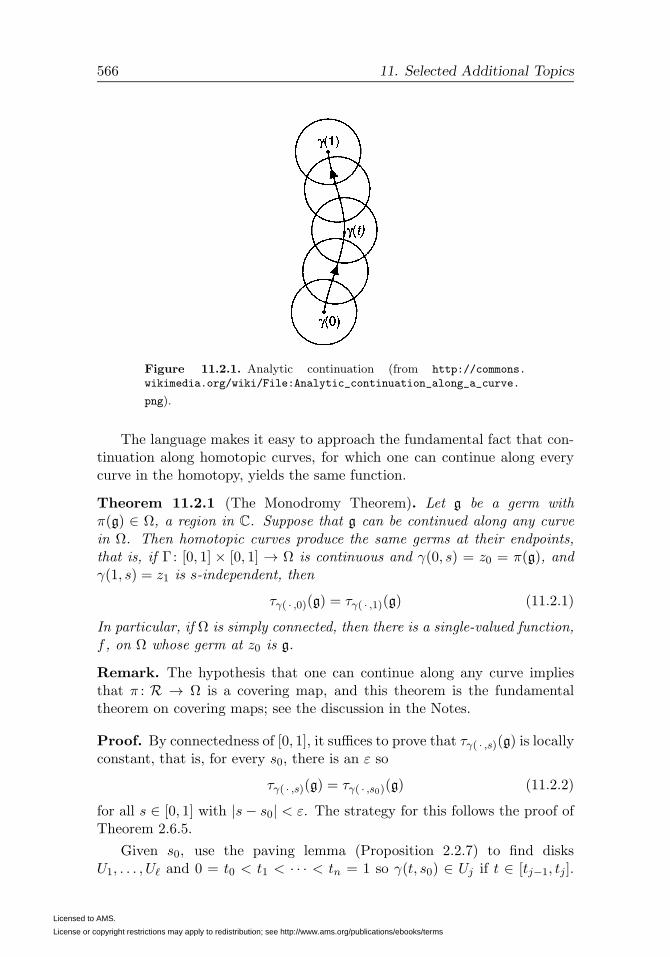
566 11. Selected Additional Topics
Figure 11.2.1. Analytic continuation (from http://commons.
wikimedia.org/wiki/File:Analytic_continuation_along_a_curve.
png).
The language makes it easy to approach the fundamental fact that con-tinuation along homotopic curves, for which one can continue along everycurve in the homotopy, yields the same function.
Theorem 11.2.1 (The Monodromy Theorem). Let g be a germ withπ(g) ∈ Ω, a region in C. Suppose that g can be continued along any curvein Ω. Then homotopic curves produce the same germs at their endpoints,that is, if Γ: [0, 1] × [0, 1] → Ω is continuous and γ(0, s) = z0 = π(g), andγ(1, s) = z1 is s-independent, then
τγ( · ,0)(g) = τγ( · ,1)(g) (11.2.1)
In particular, if Ω is simply connected, then there is a single-valued function,f , on Ω whose germ at z0 is g.
Remark. The hypothesis that one can continue along any curve impliesthat π : R → Ω is a covering map, and this theorem is the fundamentaltheorem on covering maps; see the discussion in the Notes.
Proof. By connectedness of [0, 1], it suffices to prove that τγ( · ,s)(g) is locallyconstant, that is, for every s0, there is an ε so
τγ( · ,s)(g) = τγ( · ,s0)(g) (11.2.2)
for all s ∈ [0, 1] with |s− s0| < ε. The strategy for this follows the proof ofTheorem 2.6.5.
Given s0, use the paving lemma (Proposition 2.2.7) to find disksU1, . . . , U� and 0 = t0 < t1 < · · · < tn = 1 so γ(t, s0) ∈ Uj if t ∈ [tj−1, tj].
Licensed to AMS.
License or copyright restrictions may apply to redistribution; see http://www.ams.org/publications/ebooks/terms

11.2. Global Analytic Functions 567
Then find ε so γ(t, s) ∈ Uj if |s − s0| < ε and t ∈ [tj−1, tj]. Since g can becontinued from z0 along γ( · , s0) and then throughout Uj , the Taylor seriesfor the continuation at the center of Uj gives the germ at every point in Uj .
It follows inductively in Uj that the continuation along γ( · , s0) fromz0 to γ(tj, s0) and then from γ(tj, s0) by the line to γ(tj, s) agrees withcontinuation along γ( · , s) to γ(tj, s0). Thus, (11.2.2) holds. �
The following is trivial to prove but important in applying and under-standing analytic continuation.
Theorem 11.2.2 (Permanence of Relation). Let Ω ⊂ C be a region. LetP (w0, . . . , wn, z) be a polynomial in w0, . . . , wn with coefficients analytic inz ∈ Ω. Let f be analytic in some Dδ(z0) ⊂ Ω and suppose in that disk,
P (f(z), f ′(z), . . . , f (n)(z), z) = 0 (11.2.3)
Suppose f can be analytically continued along some curve γ in Ω and let
f be the continuation in some Dγ(γ(1)). Then (11.2.3) holds for f whenz ∈ Dδ(γ(1)).
Proof. Cover γ with disks U1, . . . , Un as in the last proof and note that forany analytic function, g, on Uj , P (g(z), g′(z), . . . , z) is analytic on Uj . Thus,(11.2.3) continues disk by disk to Un. �
Finally, we want to define the representations of the homotopy groupthat is sometimes possible in special but natural situations. In Problem 3,you will prove the following:
Theorem 11.2.3 (Cauchy’s ODE Theorem). Let a0(z), . . . , an−1(z) be an-alytic in some Dδ(z0). Then for any (λ0, . . . , λn−1) ∈ Cn−1, there exists aunique analytic function on Dδ(z0), f�λ(z), that obeys
f (n)(z) +n−1∑j=0
aj(z)f(j)(z) = 0 (11.2.4)
f (j)(z0) = λj j = 0, . . . , n− 1 (11.2.5)
This sets up a one-one correspondence between Cn and all solutionsof (11.2.4).
Theorem 11.2.4. Let Ω be a region in C and a0(z), . . . , an−1(z) elementsof A(Ω). Pick z0 ∈ Ω. Then for any closed curve in Ω with γ(0) = γ(1) = z0and any solution, f , of (11.2.4) near z0, there is an analytic continuationof f along γ. γ �→ τγ(f) only depends on the homotopy class in γ. The
map (λ0, . . . , λn−1) → (g(0), . . . , g(n−1)(0)) where g = τγ(fλ0,...,λn−1) is a
Licensed to AMS.
License or copyright restrictions may apply to redistribution; see http://www.ams.org/publications/ebooks/terms

568 11. Selected Additional Topics
map (linear in (λ0, . . . , λn−1)), M[γ](λ0, . . . , λn−1) and is a representationof π1(Ω, z0) in that
M[γ]M[γ′] =M[γ,γ′] (11.2.6)
Proof. Cover γ with disks lying in Ω, using the paving lemma (Proposi-tion 2.2.7). By Theorem 11.2.3, we can continue along successive disks toget the continuation. Homotopy independence follows from Theorem 11.2.2and linearity ofM[γ] from linearity of the differential equation. (11.2.6) fol-lows from the definition of product in the homotopy group and the definitionof analytic continuation. �
The group of maps {M[γ]} is called the monodromy group. We’ll saymore about it in Chapter 14 of Part 2B. In particular, if Ω is simply con-nected, solutions define single-valued functions on all of Ω.
Theorem 11.2.5. Let Ω be a simply connected region in C anda0(z), . . . , an(z) elements of A(Ω). For each (λ0, . . . , λn−1) ∈ Cn, the uniquesolution of (11.2.4)/ (11.2.5) near z0 extends to an element of A(Ω).
The study of what happens near an isolated singularity of the aj ’s willbe a subject of Section 14.2 of Part 2B.
Notes and Historical Remarks. Starting with Riemann’s dissertation[480], the notion of Riemann surface was tied to the notion of Riemann sur-face of a function. The language of sheaves is convenient for our definitionhere—it and, in particular, its cohomology was developed for use in alge-braic geometry and in several complex variables around 1950. The pioneerswere Leray and H. Cartan, especially as part of Seminaire Henri Cartan,starting in 1950/51 [99]. Significant developments were codified in a bookof Godement [211], a student of Cartan.
Monodromy was first introduced in the context of analytic continua-tion of hypergeometric functions—solutions of a certain ODE with analyticcoefficients on C \ {0, 1}; see Sections 14.1 and 14.4 of Part 2B. The key in-novation was in a paper of Riemann [483] who thought abstractly, insteadof the rather concrete earlier work of Kummer. Hermite [255] had the ideaof associating continuation around algebraic singularities with matrices, butit was Riemann who looked at products of such matrices. Further develop-ments of monodromy groups were associated with Frobenius, Fuchs, Klein,Poincare, and Schwarz. It was Weyl in his pathbreaking book on Riemannsurfaces [590] that first went beyond monodromy groups and discussed whatis essentially the general monodromy theorem.
An especially interesting case of monodromy is where an initial germcan be continued analytically along a curve in Ω, a region, typically C witha finite set of points removed. In that case, one can connect the removed
Licensed to AMS.
License or copyright restrictions may apply to redistribution; see http://www.ams.org/publications/ebooks/terms

11.2. Global Analytic Functions 569
points by “branch cuts” and get the Riemann surface of the function as amultisheeted object over Ω. In this situation, the elements of the monodromygroup permute the sheets.
If g is a germ near z = 0 which can be continued along each ray from 0 toany z1 ∈ Dδ, then it is easy to see, using Corollary 2.3.9 and Theorem 3.1.1,that the radius of convergence of g is at least δ. This shows that if g is agerm in S(Ω) which can be continued along any curve in Ω and g1 is a τγ([g])and z1 = π(gn), then ρ(g1) is at least δ = dist(z1,C \ Ω). Therefore, themap from all germs obtained from g by continuation is a covering space forΩ with π as covering map. This shows that Theorem 11.2.1 can be provenfrom the fundamental theorem on covering maps (see Theorem 1.7.2).
For algebraic singularities, that is, if Ω is missing an isolated point, z0,and f returns to its original germ after n loops, one can show that one canadd a single point to the Riemann surface with π(p) = z0 and (z − z0)
1/n
as a local coordinate. π is no longer a covering map, but it is an analyticfunction between Riemann surfaces.
Cauchy apparently included some results on ODEs in his 1825–26 EcolePolytechnique lectures which were not widely available. In 1835, he wrote apaper [105] that summarized these results.
Problems
1. (a) Prove that if a germ, g, can be continued along a curve, γ, there isanother curve, γ, which is a piecewise linear curve, with each segmentof rational length and each slope a rational multiple of 2π, so that ifz1 = γ(1), z1 = γ(1), then z1 is in the circle of convergence of g ≡ τγ(g)and τγ(g) is the germ at z1 of the function defined by the Taylor seriesof g.
(b) Prove that the connected components of S(Ω) defined by an initialgerm, g, is a separable metric space.
2. Verify that the maps, π, on the collection Ur, define an analytic structureon R.
3. This problem will prove Theorem 11.2.3. For notational simplicity, takez0 = 0.
(a) Prove that the differential equation (11.2.4)/(11.2.5) is equivalent toa first-order vector-valued equation
y′(z) = A(z)y(z), y(z0) = y(0) (11.2.7)
where y is an n-component vector and A an n × n matrix with matrixelements also analytic in Dδ(0). (Hint: y(z) = (f(z), . . . , f (n−1)(z0)).)
Licensed to AMS.
License or copyright restrictions may apply to redistribution; see http://www.ams.org/publications/ebooks/terms

570 11. Selected Additional Topics
(b) At the level of formal power series, if
A(z) =∞∑n=0
Anzn, y(z) =
∞∑n=0
ynzn (11.2.8)
prove that (11.2.7) is equivalent to
yn+1 = (n+ 1)−1n∑
j=0
Ajyn−j , y0 = y(0) (11.2.9)
and that if the solution, {yn}∞n=0, of (11.2.10) defines a convergent powerseries in all of Dδ(0), then Theorem 11.2.3 is proven.
(c) Pick 0 < ρ < r < δ and suppose ‖An‖ ≤ ar−n for all n. Letxn = ynρ
−n. Prove that
|xn+1| ≤ (n+ 1)−1aρ
(1− ρ
r
)−1
max0≤j≤n
|xj| (11.2.10)
and conclude that supn|xn| <∞, so that the power series for yn convergesfor |z| < ρ.
(d) Complete the proof of Theorem 11.2.3.
11.3. Picard’s Theorem via the Elliptic Modular Function
Here are two spectacular theorems that we’ll prove in this section:
Theorem 11.3.1 (Picard’s Little Theorem). A nonconstant entire functiontakes every value with perhaps one exception.
The example f(z) = ez, which is never zero, shows there can be the oneexceptional value.
Theorem 11.3.2 (Picard’s Great Theorem). In any neighborhood of anisolated essential singularity, a function f takes every value with at mostone exception infinitely often.
Remarks. 1. This is also known as Picard’s Big Theorem.
2. This is a vast and deep generalization of the Casorati–Weierstrass theo-rem (Theorem 3.8.2); it was proven only eleven years later than Casorati’spublication.
Notice that the great theorem implies the little theorem, since if f(z)is entire and nonconstant, then either f is a nonconstant polynomial whichtakes every value by the fundamental theorem of algebra (Theorem 3.1.11)or else f(1/z) has an essential singularity at zero. That said, we will firstprove the little theorem below since the proof will depend on a strongerresult we need for the great theorem. However, in our two later proofs of
Licensed to AMS.
License or copyright restrictions may apply to redistribution; see http://www.ams.org/publications/ebooks/terms

11.3. Picard’s Theorem 571
these theorems (see Section 11.4 and Section 12.4 of Part 2B), we’ll onlyprove the great theorem. The key to our proof in this section is the ellipticmodular function, as used in the following:
Proposition 11.3.3. Let γ be a curve in C \ {0, 1}. Then there is a curveγ in C+ so λ ◦ γ = γ.
Remarks. 1. λ is the elliptic modular function as constructed in Section 8.3or Section 10.6.
2. This is, of course, just a consequence of the fact that λ is a covering map,but rather than use the theory of covering spaces, we use the properties ofλ as stated in Theorem 8.3.1.
Proof. Cover γ with disks Dδ(z0)(γ(t)) so λ has an inverse ηt on Dδ(t)(γ(t)).By the paving lemma (Proposition 2.2.7), we can find t0 = 0 < t1 <· · · < tn = 1, so each γ([tj−1, tj ]) ⊂ Uj , one of the Dδ(sj)(γ(sj)). Let
ηj ≡ ηsj . Define γ inductively as follows. Set γ on [t0, t1] to η1(γ(t)). Sinceλ(η1(γ(t1))) = λ(η2(γ(t1))), there is f1 ∈ Γ(2), so f1(η2(γ(t1))) = η1(γ(t1)).Define γ on [t1, t2] as f1(η2(γ(t))). Having defined γ on [tj−1, tj ] andf1, . . . , fj−1 inductively, find fj ∈ Γ(2) so fj(ηj+1(γ(tj))) = fj−1(ηj(γ(tj)))and define γ on [tj, tj+1] as fj(ηj+1(γ(t))). �Proposition 11.3.4. Let Ω ⊂ C be simply connected and let f : Ω → C \{0, 1} be analytic. Then there exists an analytic g : Ω→ C+ so that
λ(g(z)) = f(z) (11.3.1)
for all z ∈ Ω.
Remark. Again, one can use the fundamental lifting theorem for coveringspaces instead of the argument below.
Proof. Fix z0 ∈ Ω. Let γ0 be a path in Ω with γ0(0) = z0. Pick w0 ∈ C+
with λ(w0) = f(z0). Let γ(z) = f(γ0(t)) so γ is a curve in C \ {0, 1}. Let γbe a curve in C+ with λ(γ(t)) = γ(t) as constructed in Proposition 11.3.3.
Since λ(γ(0)) = γ(0) = f(z0), we have λ(w0) = λ(γ(0)), so there isα ∈ Γ(2) with α(γ(0)) = w0. λ is analytic in a neighborhood of γ, so ifwe define g(γ0(t)) = λ(α(γ(t))), g will be analytic in a neighborhood of γ0.Thus, g defined near z0 as that inverse under λ of f(z) can be continuedalong any curve. By the monodromy theorem (Theorem 11.2.1), g can bedefined on all of Ω as a single-valued function which obeys (11.3.1). �
Proof of Theorem 11.3.1. Suppose α and β are two values not taken. Byreplacing f by (f(z)− α)/(β − α)−1, we can suppose α = 0, β = 1.
Pick Ω = C in Proposition 11.3.3 and so find g : Ω→ C+ with λ ◦ g = f .Since g is entire and (g(z) + i)−1 has |(g(z) + i)−1| ≤ 1, (g(z) + i)−1 is
Licensed to AMS.
License or copyright restrictions may apply to redistribution; see http://www.ams.org/publications/ebooks/terms

572 11. Selected Additional Topics
constant and obviously nonzero, so g(z) is constant. Thus, f(z) = λ(g(z))is constant. �
Proposition 11.3.5. Let {fn}∞n=1 be a sequence of functions in A(Ω) sothat each fn takes values in C \ {0, 1}, and for some z0 ∈ Ω, fn(z0) has afinite limit in C \ {0, 1}. Then we can pass to a subsequence, fnj , whichconverges to some f in A(Ω) uniformly on compact subsets of Ω.
Proof. It is easy to pick open disks, {Um}∞m=1 in Ω which obey: (i) z0 ∈ U1;(ii)
⋃∞m=1 Um = Ω; (iii) Um+1 ∩
⋃mj=1 Uj �= ∅ (see Problem 1).
Let λ : D→ C \ {0, 1} by
λ(z) = λ
(−i(z − 1
z + 1
))(11.3.2)
Let fn(z0) = wn and let wn → w∞. Pick yn ∈ D so λ(yn) = wn and then
yn → y∞, so λ(y∞) = w∞. Pulling back Proposition 11.3.4 to D, we can
find gn : U0 → D, so gn(z0) = yn and λ(gn(z)) = fn(z).
Since the gn are uniformly bounded on U1, by Montel’s theorem (Theo-rem 6.2.2), we can find g∞ analytic in U1 and a subsequence so gnj → g∞uniformly on compact subsets of U1. Since g∞(z0) = y∞ ∈ D, by the maxi-
mum principle, Ran(g∞) ⊂ D. By continuity of λ on D, fnj → f∞ ≡ λ ◦ g∞on compacts of U1.
Since U1 ∩ U2 �= ∅, find z1 in the intersection and apply the above ar-gument to U2. Since fnj converges uniformly on U1 ∩ U2, so do the gnj
constructed in this step. Thus, by the Vitali convergence theorem (Theo-
rem 6.2.8), gnj , and so fnj = λ◦gnkconverges uniformly on compacts of U2,
and so fnj converges on compacts of U1 ∪ U2.
Iterating this argument completes the proof. �
This last proposition is a special case of the Montel three-value theorem.While it alone can be used to prove the big Picard theorem, with one extratrick, we can get the full Montel three-value theorem (see the discussionafter Theorem 6.2.10 for why it is called “three-value”):
Theorem 11.3.6 (Montel Three-Value Theorem). Let α �= β lie in C. Theset of functions f ∈ A(Ω) with Ran(f) ⊂ C \ {α, β} is a normal family.
Proof. By an argument that follows that of Proposition 11.3.5, we needonly prove this when Ω is a disk (Problem 2) and by replacing fn by (fn −α)/(β −α), we can suppose α = 0, β = 1. Thus, we are reduced to showingthat any sequence of functions, fn, in A(D) with values in C \ {0, 1} eitherhas a limit in A(D) or converges uniformly to ∞.
Licensed to AMS.
License or copyright restrictions may apply to redistribution; see http://www.ams.org/publications/ebooks/terms

11.3. Picard’s Theorem 573
Since C is compact, by passing to an initial subsequence, we can suppose
fn(0) → w∞ ∈ C. If w∞ ∈ C \ {0, 1}, then by Proposition 11.3.5, fn has aconvergent subsequence.
Suppose next that w∞ = 1. Since fn is never zero, we can let gn =√fn, taking the square root with fn(0) near −1. Then gn has a convergent
subsequence, and thus, so does fn = g2n. Indeed, by Hurwitz’s theorem(Corollary 6.4.2), the subsequence must converge to f∞ ≡ 1.
If w∞ = 0, gn = 1− fn has a subsequence converging, and then f∞ ≡ 0by the above. Finally, if w∞ =∞, gn = 1−f−1
n has a convergent subsequenceand f∞ ≡ ∞ by the above. �
Proof of Theorem 11.3.6 ⇒ Theorem 11.3.2. Define gn on A 12,2 by
gn(z) = f(4−nρz) where ρ is such that f is analytic in D 12ρ(0)\{0}. By The-
orem 11.3.6, there is a subsequence gnj , so either gnj converges uniformly
on ∂D or g−1nj
converges to 0. In particular, either
sup|z|=1j
|gnj(z)| = S <∞ or lim|z|=1j→∞
|gnj(z)−1| = 0
In the first case, f is uniformly bounded on the circles of radius4−njρ. But, by the maximum principle, the maximum on each annulusA4−nj−1ρ,4−nj ρ
occurs on one of these circles, so f is bounded near 0 and so
has a removable, not essential, singularity.
In the second case, applying the argument to f−1, we show (recall fis never 0) limz→ 0 f(z)
−1 = 0, so 0 is a polar singularity, not an essentialsingularity. �
Notes and Historical Remarks. Picard’s theorems were proven, oneshortly after the other, in 1879 (announcements in [431, 432] and full pa-per in [433]). His proofs relied on the elliptic modular function, albeitwithout the language of normal families. For a modern version of the proofin language closer to Picard, see Ullrich [559] and Veech [562]. See theNotes to Section 6.2 for the history of Montel’s three-value theorem.
Schiff [503] has extensive discussion of the history of normal familiesand various wrinkles in the proofs in this section.
Julia [295] has proven the following strengthening of the great Picardtheorem:
Theorem 11.3.7 (Julia’s Theorem). Let f be analytic in some Dρ\{0} andhave an essential singularity at zero. Then there exists a direction eiθ0 ∈ ∂Dso that for every ε > 0, f(z) takes infinitely often every value, with at mostone exception on the set {z = reiθ | 0 < r < 1, |θ − θ0| < ε}.
Licensed to AMS.
License or copyright restrictions may apply to redistribution; see http://www.ams.org/publications/ebooks/terms

574 11. Selected Additional Topics
For a proof that uses no more than Montel’s three-value theorem, seeMarkushevich [373, Ch. III, p. 344], Saks–Zygmund [500, p. 352], or Schiff[503, p. 62].
Picard’s theorem has evoked considerable interest in regard to extendingit to other contexts. One extension involves projective curves, that is, maps
of C to CP(n). CP(1) = C, so Picard’s theorem deals with the case n = 1.A hyperplane, H, in CP(n) is parameterized by a ∈ Cn+1 \ {∞} via
H =
{[(z1, . . . , zn+1)]
∣∣∣∣ n+1∑j=1
ajzj = 0
}(11.3.3)
For n = 1, Picard’s theorem says ifH1, H2, H3 are three distinct hyperplanes(hyperplanes are points) and f : C → CP[1] has Ran(f) ∩ Hj = ∅, then
f is constant. Cartan [95, 98] has proven that if {Hj}2n+1j=1 are 2n + 1
hypersurfaces in CP[n] with ⋂j∈I
Hj = ∅ (11.3.4)
for any I ⊂ {1, . . . , 2n + 1} with #(I) = n + 1 and if f : C → CP[n] isholomorphic with Ran(f)∩Hj = ∅ for j = 1, . . . , 2n+1, then f is constant.See also [166, 167]. Cartan proved and used an extension of Nevanlinnatheory. The reader will prove this result in Problem 2 of Section 3.3 ofPart 3.
There is also a Picard-type theorem for so-called quasiregular maps onRn; see Rickman [479] and Eremenko–Lewis [168].
Emile Picard (1856–1941) was a French mathematician whose life wasimpacted by war. His father died during the 1870 siege of Paris in theFranco–Prussian war and his mother struggled to put her two sons throughlycee. Both of his sons were killed on the front in the First World War(Picard’s student, Hadamard, also lost two sons in that war).
Picard spent almost his entire career in Paris, although his wonderfultheorems we discuss in this section were done during a two-year period whenhe taught in Toulouse. His advisor was Darboux and, in turn, his studentsinclude Bernstein, Hadamard, Julia, Painleve, and Weil.
His signature theorems relied on the elliptic modular function used ear-lier by his teacher and father-in-law, Hermite, in his solution of quintics (al-though Picard did this work two years before he married Hermite’s daugh-ter). Picard is also noted for his work on ordinary differential equations,in particular, his existence theorem that relied on iteration of the integralequation.
Problems
1. Let z0 ∈ Ω ⊂ C be a region. Prove there exist open disks {Um}∞m=1
covering Ω so z0 ∈ U1 and so Um+1 ∩⋃m
j=1 Uj �= ∅.
Licensed to AMS.
License or copyright restrictions may apply to redistribution; see http://www.ams.org/publications/ebooks/terms

11.4. Zalcman’s Lemma 575
2. Let {fn}∞n=1 be a sequence of functions analytic on Ω ⊂ C. Let z0 ∈ Ωand let {Un}∞n=1 be a cover as constructed in Problem 1 and so that anysubsequence of the fn has a subsubsequence converging in A(Un). Provethere is a subsequence converging in A(Ω).
11.4. Bonus Section: Zalcman’s Lemma and Picard’sTheorem
In the twenty years following 1896, there appeared a number of approaches toPicard’s theorems that replaced elliptic functions with rather explicit boundson families of functions. Here we’ll present a rather recent twist on theseideas that avoids explicit bounds by using an elegant lemma of Zalcman.We’ll heavily use bonus Section 6.5 via the use of the spherical metric, thespherical derivative, f �, of (6.5.25) and Marty’s theorem (Theorem 6.5.6).Here is the key construct:
Proposition 11.4.1 (Zalcman’s Lemma). Let S be a family of meromorphicfunctions on a region, Ω ⊂ C, which is not normal. Then there exists{fn}∞n=1 ⊂ S, zn ∈ Ω, zn → z∞ ∈ Ω, and nonnegative numbers ρn → 0 sothat if
gn(ζ) = fn(zn + ρnζ) (11.4.1)
then for some entire meromorphic function, g∞, we have
(i) gn → g∞ normally on each DR with R <∞.
(ii) g�∞(0) = 1 so, in particular, g∞ is not constant.
(iii) g�∞(ζ) ≤ 1 for all ζ ∈ C.
Moreover, if V ⊂ C is such that Ran(fn) ⊂ V for all n, then Ran(g∞) ⊂ V.
Proof. The key to the proof is that
g�n(ζ) = ρnf�n(zn + ρnζ) (11.4.2)
Once one has the idea of looking at max((1 − |z|2)f �n(z)), the details are
straightforward—at least once one knows the result is true. Throughout, wepick subsequences but continue to use fn for the subsequences.
By Marty’s theorem and the assumed non-normality, there exists a com-pact K ⊂ Ω so that supf∈S, z∈K‖f �(z)‖ =∞. Thus, there is wn → w∞ ∈ Kand fn ∈ S so that
f �n(wn) ≥ n (11.4.3)
For simplicity of notation, suppose w∞ = 0 and that D ⊂ Ω. By trans-lation and scaling, we can certainly arrange that. Define
Mn = sup|z|≤1
(1− |z|2)f �n(z) (11.4.4)
Licensed to AMS.
License or copyright restrictions may apply to redistribution; see http://www.ams.org/publications/ebooks/terms

576 11. Selected Additional Topics
By (11.4.3), Mn ≥ (1 − |wn|2)n → ∞ since wn → 0. Moreover, since thefunction of z, whose sup is taken, is continuous and vanishing on ∂D, thereis zn ∈ D so (1− |zn|2)f �
n(zn) = Mn, and by passing to a subsequence, thatzn → z∞ ∈ D ⊂ Ω.
Define ρn by
ρn = [f �(zn)]−1 = M−1
n (1− |zn|2) ≤M−1n → 0 (11.4.5)
Moreover,
(1− |zn|)−1ρn = M−1n (1 + |zn|) ≤ 2M−1
n (11.4.6)
Thus, for R fixed and n so large that R < 12Mn, we have
|ζ| ≤ R⇒ |zn + ρnζ| < 1 (11.4.7)
Define gn by (11.4.1) on the set where |zn + ρnζ| < 1. By (11.4.2),
|g�n(0)| = ρn[f�n(zn)] = 1 (11.4.8)
and
|g�n(ζ)| ≤ ρnf�n(zn + ρnζ)
≤ ρnMn(1− |zn + ρnζ|2)−1
=1− |zn|2
1− |zn + ρnζ|2(11.4.9)
≤ 1 + |zn|1 + |zn|+ ρn|ζ|
1− |zn|1− |zn| − ρn|ζ|
(11.4.10)
≤ 1
1− 2|ζ|M−1n
(11.4.11)
so long as |ζ| < 12Mn. In the above, we go from (11.4.9) to (11.4.10) using
|zn+ρnζ|2 ≤ (|zn|+ρn|ζ|)2 and (1−a2) = (1−a)(1+a). We go from (11.4.10)to (11.4.11) since the first term is bounded by 1 and ρn|ζ|(1 − |zn|)−1 ≤2|ζ|M−1
n by (11.4.6).
Thus, we have proven for each fixed R,
limn→∞
sup|ζ|≤R
g�n(ζ) = 1 (11.4.12)
That means, by Marty’s theorem, we can arrange g∞ meromorphic on C anda subsequence, also denoted gn, so that gn → g∞ uniformly on compactsof C. Moreover, (ii) and (iii) hold by (11.4.8) and (11.4.12).
Since g�∞(0) = 1, g�∞ is not constant, so by Hurwitz’s theorem, g∞cannot take any value not taken by any fn. In particular, g∞ does not takethe value ∞ if all f ∈ S are analytic. �
Licensed to AMS.
License or copyright restrictions may apply to redistribution; see http://www.ams.org/publications/ebooks/terms

11.4. Zalcman’s Lemma 577
Proof of Montel’s Three-Value Theorem. By Problem 2 of Sec-tion 11.3, we need only prove the result for simply connected Ω. Fix α, β, γ
distinct in C and let Mα,β,γ(Ω) be the set of all meromorphic functions(or f ≡ ∞) that never take the value α, β, or γ. We need to prove
Mα,β,γ(Ω) is normal. If F is any element of Aut(C), it is easy to see thatMF (α),F (β),F (γ)(Ω) is normal if and only if Mα,β,γ(Ω) is (Problem 1). Sowithout loss, we can take α = 0, β = 1, γ = ∞, that is, look at S, thosef ∈ A(Ω) which are never 0 or 1. Let Sk be a set of functions in A(Ω) thatnever take the value 0 or any of 2k-th roots of unity.
Fix k for a moment. If fn is a sequence in S, pick gn = f1/2k
n where wetake any of the analytic 2k-th roots guaranteed by Theorem 2.6.1 and the
assumption that Ω is simply connected. If gnj is convergent, so is fnj = g2k
nj.
So if S is not normal, so is each Sk.
If Sk is not normal, by Zalcman’s lemma, there exist entire functions,
g(k)∞ , obeying (i) (g
(k)∞ )�(0) = 1; (ii) (g
(k)∞ )�(z) ≤ 1 for all z; (iii) g
(k)∞ does not
take the value 0 or any 2k-th root of unity.
By Marty’s theorem, there is a subsequence converging to an entire
function g∞ with (i) g�∞(0) = 1 (so g∞ is not constant); (ii) g�∞(z) ≤ 1for all z; (iii) by Hurwitz’s theorem, g∞ does not take any value eiθ whereθ/2π is a dyadic rational. By the open mapping theorem, |g∞(z)| �= 1 forall z. Thus, by continuity, either |g∞(z)| < 1 for all z or |g∞(z)−1| < 1 forall z. Either way, by Liouville’s theorem, g∞ is constant, inconsistent with
g�∞(0) = 1. This contradiction shows that S is normal. �
Once we have Montel’s three-value theorem, we get Picard’s theoremsas in Section 11.3.
Notes and Historical Remarks. These Notes will discuss what havecome to be called “elementary” proofs of the Picard theorems, a term thatseems to go back to Borel [65]. “Elementary” does not mean simple, lessinvolved, or more natural. For the prime number theorem, the phrase is usedfor proofs that do not use complex analysis. It is difficult to imagine proofsof Picard’s theorems that don’t use complex analysis (but see Section 3.3of Part 3). The term seems to mean proofs that don’t use “fancy stuff”—initially that meant not using elliptic functions. Somehow the Ahlfors–Robinson proof (see Sections 12.3 and 12.4 of Part 2B), which uses curvaturein conformal Riemann metrics, doesn’t qualify for “elementary”!
Traditionally, it applied to proofs of Landau, Schottky, and Bloch thatwe turn to below. Those traditional proofs are not especially simpler thanthe elliptic modular function or Ahlfors–Robinson proofs. The proof viaZalcman’s lemma is their descendant and it is undoubtedly the shortest
Licensed to AMS.
License or copyright restrictions may apply to redistribution; see http://www.ams.org/publications/ebooks/terms

578 11. Selected Additional Topics
proof from first principles (although the Nevanlinna theory (see Section 17.3of Part 2B) and the Eremenko–Sodin proof (see Section 3.3 of Part 3) arefairly direct). One can argue that the essence of the Picard theorem is thatC\{0, 1} has a universal cover that supports bounded nonconstant functionsand, in that sense, the proof that relies on elliptic modular functions is mostelementary.
Zalcman’s lemma is from a 1975 paper [600]. Not surprisingly, itgenerated considerable followup, summarized in Zalcman [601]. Earlier,Lohwater–Pommerenke [365] had used a similar construction but for sin-gle functions on D obeying sup|z|(1 − |z|2)f �(z) < ∞ (such functions are
called normal functions) rather than families. The elegant argument we useto prove Montel’s three-value theorem from Zalcman’s lemma is from Ros[491]. The general idea of multiplying by (1 − |z|2) used in the proof ofZalcman’s lemma is due to Landau [341].
Zalcman’s lemma can be used to prove other normality results, for ex-ample (see Problem 2), the following theorem of Caratheodory [90]: If Sis a family of meromorphic functions on Ω ⊂ C, a region so that there arethree values α(f), β(f), γ(f), not taken by f (but f -dependent) and
inff∈S
[min(σ(α(f), β(f)), σ(β(f), γ(f)), σ(γ(f), α(f)))]> 0 (11.4.13)
then S is normal.
There is a general principle that has been used as a guide to the studyof normality—often called Bloch’s principle. The idea is that if a propertyforced on entire functions causes the function to be constant, then thatproperty on a family of functions on a region forces the family to be normal.Schiff [503] presents an explicit version of this, proved by Zalcman whowas motivated in part by trying to provide a basis for this principle assuggested by Abraham Robinson. The name “Bloch’s principle” comes fromthe statement in his paper [55] (the original quote is in Latin): “There isnothing in the infinite which did not exist before in the finite.”
The first proof of a Picard theorem without elliptic modular functionswas by E. Borel [65] in 1896. Seventeen years after Picard’s work, he foundan “elementary” proof of the little Picard theorem. It was Schottky [506]in 1904, motivated in part by the earlier work of Borel and of Landau [338],who found the first “elementary” proof of the great Picard theorem; heshowed:
Theorem 11.4.2 (Schottky’s Theorem). For each a ∈ C and θ ∈ (0, 1),there is a constant C(a, θ) so that if f ∈ A(DR) with f(0) = a and Ran(f) ⊂C \ {0, 1}, then
sup|z|≤θR
|f(z)| ≤ C(a, θ) (11.4.14)
Licensed to AMS.
License or copyright restrictions may apply to redistribution; see http://www.ams.org/publications/ebooks/terms

11.4. Zalcman’s Lemma 579
It is fairly easy to see (Problem 3) that this result is equivalent to Mon-tel’s three-value theorem, so it is not difficult to believe it led to a proof ofthe great Picard theorem.
A new element was introduced by Bloch [54] in 1924 (when he publishedan announcement). He proved the remarkable
Theorem 11.4.3 (Bloch’s Theorem). For any nonconstant analytic func-tion f in a neighborhood of D, let b(f) be the sup of the radii of all disks,Df(z0)(ρ), in Ran(f) which are a bijective image of f restricted to a subdo-main of D. Then there is a lower bound, b, on {b(f) | f ′(0) = 1}.
We emphasize that while the normalization is at 0, the z0 need notbe f(0) and, indeed, there is no uniform lower bound on disks about f(0)which are bijective images. Bloch also relates this result to Picard’s littletheorem. b is called Bloch’s constant. A related number is Landau’s constant(named after Landau [341]), the inf of the order of the radius of largest diskin Ran(f), known to be strictly larger than Bloch’s constant. There isconsiderable literature on these constants, including conjectured values; seeFinch [188, Sec. 7.1].
For further discussion of Schottky’s and Bloch’s theorems, includingproofs, see Conway [120], Remmert [477], and Titchmarsh [556].
Andre Bloch (1893–1949) had a tragic life. In 1917, while on leave fromthe French army, he murdered his brother, his aunt, and his uncle. All hispapers were written while he was resident in an asylum for the criminallyinsane.
Problems
1. Let fn be a sequence of meromorphic functions on Ω. Let F be a fixed
element of Aut(C). Prove F ◦ fn has a normal limit (in the sense ofSection 6.5) if and only if fn does.
2. Let S be a family of functions on a region, Ω, so that each f ∈ S ismissing three values, α(f), β(f), γ(f), possibly f -dependent, but so that(11.4.13) holds. Prove the theorem of Caratheodory that S is normal.(Hint: Use Zalcman’s lemma but show, by passing to a subsequence, you
can arrange that α(gn), β(gn), γ(gn) each have limits in C with the ρ-metric and these limits are unequal. Then use the little Picard theoremon the limit.)
3. (a) Use the Montel three-value theorem to prove Schottky’s theorem(Theorem 11.4.2).
(b) Conversely, assuming Schottky’s theorem, prove the three-value the-orem.
Licensed to AMS.
License or copyright restrictions may apply to redistribution; see http://www.ams.org/publications/ebooks/terms

580 11. Selected Additional Topics
4. Let f be an entire function and suppose f ◦ f has no fixed points. You’llprove that f(z) = z + b for some b.
(a) Show g(z) = (f(f(z))−z)/(f(z)−z) is an entire function which nevertakes the value 0 or 1 and so is a nonzero constant c.
(b) Prove that f ′(f(z)) never takes the values c or 0 (Hint: Prove thatf ′(z)[f ′(f(z))− c] = 1− c) and conclude that f(z) = az+ b for some a, b.
(c) Prove that f(z) = z + b.
5. Prove that if f and g are entire functions and ef + eg = 1, then f and gare both constant.
6. Consider the family on C, S = {fn(z)}n=0,1,2,... where fn(z) = zn.
(a) Prove that S is not normal.
(b) Prove that in Zalcman’s lemma, one can pick zn ≡ 1, ρn = 2/n.What is g∞? Check that this g∞ obeys (ii) and (iii) of Zalcman’s lemma.
11.5. Two Results in Several Complex Variables:Hartogs’ Theorem and a Theorem of Poincare
Here we want to focus on two results about several complex variables. In C,a fundamental role is played by the unit disk D. On Cn, one issue is thatthere are (at least) two natural candidates to replace D:
Definition. In Cn, the polydisk, Dn, is defined by
Dn ={z = (z1, . . . , zn) ∈ Cn
∣∣ maxj=1,...,n
|zj| < 1}
and, more generally, Dnr (z0) is defined by making the condition
maxj=1,...,n|zj − z(0)j | < r. The ball is defined by
Bn =
{z ∈ (z1, . . . , zn) ∈ Cn
∣∣∣∣ |z| = ( n∑j=1
|zj|2)1/2
< 1
}A region, Ω ⊂ Cn, is an open connected set and f : Ω → C is called
analytic on Ω if there is a convergent multivariable power series about eachz(0) ∈ Ω, that is, for some r > 0 and all z ∈ Dr(z
(0)), we have
f(z) =
∞∑j1,...,jn=0
aj1...jn(z1 − z(0)1 )j1 . . . (zn − z(0)n )jn
converging uniformly on Dr(z(0)). An analytic or conformal equivalence is
a bijection Ω1 → Ω2 so that each component is analytic.
Many results from one variable extend (see Problems 9 and 10). Wewant to focus here on two significant differences:
Licensed to AMS.
License or copyright restrictions may apply to redistribution; see http://www.ams.org/publications/ebooks/terms

11.5. Two Results in Several Complex Variables 581
Theorem 11.5.1 (Hartogs’ Theorem). If f is analytic on D21(0) \ D2
1/2(0),
then f has a continuation to all of D21(0).
Theorem 11.5.2 (Poincare’s Theorem). B2 and D2 are not conformallyequivalent.
Of course, the situation in C is very different. If f ∈ A(D) has a naturalboundary on ∂D, then g(z) = f(z) − f(12z
−1) is analytic on A 12,1 and no
bigger region, and while any two simply connected regions in C are confor-mally equivalent, both B2 and D2 are simply connected and topologicallytrivial by all meanings of that notion.
Proof of Theorem 11.5.1. For each w ∈ D, let gw(z) = f(z, w) where gis defined on D for 1
2 < |w| < 1 and on A 12,1 for |w| ≤ 1
2 . Thus,
gw(z) =∞∑
n=−∞an(w)z
n (11.5.1)
converging for z ∈ A 12,1 and
an(w) =1
2πi
‰|z|= 3
4
z−n−1f(z, w) dz (11.5.2)
By the Cauchy theorem,
n ≤ −1 and 12 < |w| < 1⇒ an(w) = 0 (11.5.3)
but by (11.5.2), an(w) is analytic for w ∈ D. It follows that an(w) = 0for n < 1, so (11.5.1) converges for all z ∈ D, w ∈ D, that is, f has a
continuation to all of D(2)1 (0). �
Theorem 11.5.2 is somewhat more subtle. For 0 ∈ Ω ⊂ C2, defineAut0(Ω) to be the analytic bijections, f , of Ω with f(0) = 0. We’ll provethat Aut0(B2) and Aut0(D2) are very different and use that to prove the tworegions cannot be conformally equivalent. As preparation,
Theorem 11.5.3 (Cartan’s First Theorem). Let Ω ⊂ C2 be bounded with0 ∈ Ω and f ∈ Aut0(Ω) obey
Df(0) = � (11.5.4)
Then f(z) ≡ z.
Remark. By Df , we mean the 2× 2 matrix
Df =
(∂f1/∂z1 ∂f1/∂z2∂f2/∂z1 ∂f2/∂z2
)(11.5.5)
where f1, f2 are the components of f .
Licensed to AMS.
License or copyright restrictions may apply to redistribution; see http://www.ams.org/publications/ebooks/terms

582 11. Selected Additional Topics
Proof. The one-variable result appears in Problem 8 of Section 7.4. Thisproof is essentially the same; see Problem 1. �
Theorem 11.5.4 (Cartan’s Second Theorem). Let Ω ⊂ C2 be a regionwith 0 ∈ Ω and the property that z ∈ Ω⇒ eiθz ∈ Ω for all eiθ ∈ ∂D. Letf ∈ Aut0(Ω). Then for some 2× 2 matrix A, f(z) = Az.
Proof. Let Qθ(z) = eiθz. By hypothesis, Qθ is an automorphism of Ω
that leaves 0 fixed. Moreover, DQθ = ( eiθ 00 eiθ
) is a multiple of �. Thus,
D(Q−1θ f−1Qθf)(0) = (DQθ)
−1(Df)−1(DQθ)(Df) = (Df)−1Df = �. So by
Theorem 11.5.3, Q−1θ f−1Qθf is the identity, that is,
Qθf = fQθ (11.5.6)
Write f(z) = (f1(z), f2(z)) and for z near zero,
fj(z) =∞∑
k,�=1
b(j)k� z
k1z
�2 (11.5.7)
Then, by (11.5.6), eiθb(j)k� = b
(j)k� e
i(k+�)θ, which means b(j)k� = 0 for (k+�) �= 1,
that is, f is linear near zero. By analyticity, f is linear. �
Theorem 11.5.5. We have that
Aut0(B2) = {f(z) = Az | A ∈ U(2), the 2× 2 unitary matrices} (11.5.8)
Aut0(D2) =
{f(z) = Az
∣∣∣∣ A =
(eiθ1 00 eiθ2
)or A =
(0 eiθ1
eiθ2 0
)}(11.5.9)
Remark. In Problem 2, the reader will find Aut(B2) and Aut(D2).
Proof. Both domains are invariant under z → eiθz so Theorem 11.5.4 ap-plies. B2 is the unit ball in Euclidean norm, so (Problem 3) A[B2] = B2 ifand only if ‖Au‖2 = ‖u‖2, and that happens if and only if A is unitary. Thisproves (11.5.8).
Let A : [D2] ⊂ D2 for a linear map A = ( a11 a12a21 a22 ). D2 is the unit ball in
‖z‖∞ = max(|z1|, |z2|) so A[D2] ⊂ D2 if and only if ‖Az‖∞ ≤ ‖z‖∞, whichholds if and only if (see Problem 4),
|a11|+ |a12| ≤ 1, |a21|+ |a22| ≤ 1 (11.5.10)
On the other hand, since A[D2] = D2, we must have that A[∂D2] = ∂D2,
so ‖A(10
)‖∞ = 1, that is,
max(|a11|, |a21|) = 1 = max(|a12|, |a22|) (11.5.11)
Licensed to AMS.
License or copyright restrictions may apply to redistribution; see http://www.ams.org/publications/ebooks/terms

11.5. Two Results in Several Complex Variables 583
These last two equations imply
|a11| = |a22| = 1; |a12| = |a21| = 0 or |a12| = |a21| = 1; |a11| = |a22| = 0(11.5.12)
which proves (11.5.9). �
Proof of Theorem 11.5.2. For any z(0) ∈ D2, let
fz(0)(z) =
(z1 − z
(0)1
1− z(0)1 z1
,z2 − z
(0)2
1− z(0)2 z2
)Then f ∈ Aut(D2) and f(z(0)) = 0. Thus, if g : B2 → D2 is an analyticbijection, h ≡ fg(0) ◦ g is an analytic bijection with h(0) = 0, so we needonly show there is no such analytic bijection.
If h is such a bijection, F → hFh−1 maps Aut0(B2) bijectively toAut0(D2). Since
D(hFh−1)(0) = (Dh)(0)DF (0)Dh(0)−1 (11.5.13)
this sets up a continuous bijection of U(2) and {A | A = ( eiθ1 00 eiθ2
) or
A = ( 0 eiθ1eiθ2 0
). Since one of these sets is connected (Problem 5) and theother is not, this cannot be. This contradiction proves the sets are notanalytically equivalent. �
Notes and Historical Remarks. Friedrich Hartogs (1874–1943) wasborn in Belgium to a prosperous German-Jewish merchant family and spenthis youth and career in Germany. He was a student of Pringsheim in Mu-nich. His great paper [242], which made him the father of several complexvariables, was his Habilitationschrift. Hartogs was also the first to use sub-harmonic functions in one complex variable theory.
He started teaching in Munich after this work. He was cautious bynature and, in 1922, turned down a full professorship in the new privateuniversity in Frankfurt because of the hyperinflation and concerns that theposition might be less secure. Finally, in 1927, he was made a professor,after pressure from his colleagues at Munich, Caratheodory, Perron, andTietze.
With the rise of the Nazis, he was dismissed. In the late thirties, he spentsome time in Dachau. His wife was Aryan so he transferred their home toher, but when the laws allowed confiscation of the property of spouses ofJews, he divorced his wife although they continued to live together. Finally,in 1943, concerned about his situation and the future, he committed suicide,like Hausdorff, via an overdose of barbiturates.
His long great paper [242] included not only Theorem 11.5.1 but also atheorem that if f is analytic in each variable with the others fixed, it is jointly
Licensed to AMS.
License or copyright restrictions may apply to redistribution; see http://www.ams.org/publications/ebooks/terms

584 11. Selected Additional Topics
analytic. This result is often called Hartogs’ theorem, and Theorem 11.5.1called Hartogs’ ball theorem (often, even in English, Kugelsatz). The namecomes from the fact that the same argument (Problem 7) proves that if fis analytic in a neighborhood of ∂B2, it has an analytic continuation to allof B2. In fact [242], Hartogs proved by the same method that
Theorem 11.5.6 (Hartogs). Let Ω be a region in Cn for n ≥ 2 and letK ⊂ Ω be compact. Then any function analytic in Ω \ K has an analyticcontinuation to Ω.
Modern approaches to Hartogs’ theorem and its extensions use ideasdifferent from the one we present (which is Hartogs’ original idea). One,due to Bochner [58] and Martinelli [374], depends on multivariable variantsof the Pompeiu formula (2.7.7) and first proves that if K is compact andf analytic and bounded on C2 \ K, then f is constant on the unboundedcomponent of C2 \ K. Another idea, due to Ehrenpreis [159], uses PDEmethods, exploiting special properties of the CR equations in higher dimen-sions. Range [469] has more history and sketches of the ideas. There is apedagogical discussion in Scheidemann [502].
One well-known theorem on analytic continuation in higher dimension,due to Bochner [57], concerns tubes, that is, sets of the form
J (K) = {z ∈ Cn | Im z ∈ K} for some K ⊂ Rn (11.5.14)
Theorem 11.5.7 (Bochner Tube Theorem). If f is analytic in J (K) forsome open K in Rn, it has an analytic continuation to the interior of theconvex hull of J (K).
This result has connections to the Paley–Wiener theorem (see Prob-lem 8).
Note that Theorem 11.5.1 says that all local singularities are removable.In general, zeros and also singularities are (n− 1) (complex)-dimension ob-jects that are sometimes hypersurfaces but can be more complicated.
Poincare’s theorem is from [443] and Cartan’s two theorems from [96].What we called Cartan’s first theorem is often called the Cartan uniquenesstheorem.
Henri Cartan (1904–2008), who lived to be 104, was the son of ElieCartan, who is noted for his work on Lie algebras, Lie groups, and differentialgeometry. Henri’s brother served in the French resistance in the SecondWorld War and was captured and executed by the Germans. Henri Cartanwas the central figure in several complex variables from 1930 to 1970, withcontributions to the more classical aspects but also to sheaf theory andmethods of homology. His book with Eilenberg, Homological Algebra, was amilestone in more than analysis. He was a founding member of Bourbaki.
Licensed to AMS.
License or copyright restrictions may apply to redistribution; see http://www.ams.org/publications/ebooks/terms

11.5. Two Results in Several Complex Variables 585
He was a student of Montel and, in turn, his students included P. Cartier,J. Cerf, J. Deny, A. Douady, R. Godement, J.-L. Koszul, J.-P. Serre, andR. Thom. The last two both finished in 1951 and both went on to win FieldsMedals.
There are a variety of approaches to the study of several complex vari-ables, and the classical considerations of this section are not typical—rathersheaf theories, PDE and integral equation techniques have been used. See[36, 100, 215, 227, 268, 330, 403, 468, 497, 502] for monograph pre-sentations.
There is also a theory of analytic functions on infinite-dimensionalspaces, going back at least to Volterra [566]. For a discussion of the modernview and a history of its development, see Dineen [143].
Problems
1. (a) For z ∈ Dnδ (0), suppose f(z) = z + Ak(z) + O(|z|k+1), where k ≥ 2
and Ak is homogeneous of degree k and nonzero. Prove inductively thatf [n](z) = z + nAk(z) +O(|z|k+1).
(b) If Ω ⊂ Cn is bounded and g : Ω → Ω has g(z) =∑∞
k=0Ak(z) as itsTaylor expansion at zero, where Ak is homogeneous of degree k, provea priori bounds (k-dependent but g-independent) on ‖Ak‖ depending onlyon Ω. (Hint: Cauchy estimates.)
(c) Prove Cartan’s first theorem.
2. (a) For any w ∈ D2, prove
fw(z) =
(z1 − w1
1− w1z1,z2 − w2
1− w2z2
)is in Aut(D2).
(b) Prove that every g in Aut(D2) can be uniquely written as g(z) =A[Fw(z)] where w ∈ D2 and A ∈ Aut0(D2).
(c) For any a ∈ D, prove that
ha(z) =
(z0 − a
1− az0,(1− |a|2)1/2z2
1− az1
)is in Aut(B2).
(d) Prove that any g in Aut(B2) can be written g(z) = Uha(V z) for 2×2unitary U, V and a ∈ D.
Remark. This decomposition is not unique.
3. Let A be a linear map on Cn. Prove the following are equivalent:(1) A[Bn] = Bn
(2) ‖Az‖2 = ‖z‖2 for all z.(3) 〈Az,Aw〉 = 〈z, w〉 for all z, w ∈ Cn where 〈z, w〉 =
∑nj=1 zjwj .
Licensed to AMS.
License or copyright restrictions may apply to redistribution; see http://www.ams.org/publications/ebooks/terms

586 11. Selected Additional Topics
4. Prove that if A = (ajk) is an n× n complex matrix, then A[Dn] ⊂ Dn ifand only if supj
∑nk=1|ajk| ≤ 1.
5. Prove that U[2] is connected. (Hint: See Problem 19 in Section 7.3.)
6. Extend Theorem 11.5.5 and Problem 2 to Cn.
7. (a) Use the method we gave for the proof of Theorem 11.5.1 to show that
if f is analytic in some B2r1(0) \B2
r2(0) for r2 < r1, then f has an analytic
continuation to B2r1(0).
(b) Prove that if f is analytic in a neighborhood of ∂B2, it has a contin-uation to B2.
8. (a) Let g be in L2(Rν). Prove that {a ∈ Rν |´|ea·xg(z)|2 dνx < ∞} is
convex.
(b) Prove the special case of Theorem 11.5.7 for f ’s that are boundedand analytic on J (K). (Hint: Let h(z) = (z−z0)
−νf(z) for some z0 �= Kand use the Paley–Wiener theorem in both directions.)
Remark. The idea here was used by Bochner [56] a year before he provedthe more general Theorem 11.5.7.
9. (a) Prove that if Ω is a region in Cn and f, g are analytic in Ω and agreenear some z0 ∈ Ω, they agree on all of Ω.
(b) Let n ≥ 2 and let f be analytic and bounded on Cn \ Kfor some compact K. Show first that for some R and each zj ,
f(z(0)1 , . . . , z
(0)j−1, zj, z
(0)j+1, . . . , z
(0)n ) is constant as zj is varied for each fixed
z(0)1 , . . . , z
(0)j−1, z
(0)j+1, . . . , z
(0)n ) ∈ Cn−1 with |z(0)k | > R. Conclude that f is
constant.
10. (a) Prove a maximum principle for analytic functions of n variables.
(b) Prove an open mapping theorem for analytic functions of n variables.
11.6. Bonus Section: A First Glance atCompact Riemann Surfaces
Here we want to describe the basic facts about meromorphic functions ongeneral compact Riemann surfaces. Because it would require considerabledevelopment of the needed machinery, there will not be any proofs and onlya few indications of the constructions. Since we will not provide any proofsand we have been careful to only place in the Notes stated theorems we don’tprove (even in the Problems), we’ll present the results in this section as aseries of “Facts.” The Notes will have references on where to find detailed
Licensed to AMS.
License or copyright restrictions may apply to redistribution; see http://www.ams.org/publications/ebooks/terms

11.6. A First Glance at Compact Riemann Surfaces 587
presentations and proofs. We include this section because it both indicatesfurther directions and really illuminates the theorems of Section 10.3.
Fact 11.6.1. Every compact two-dimension oriented manifold (and there-fore, in particular, every compact Riemann surface) is topologically equiv-alent (aka homeomorphic to) a sphere with � handles. � is called the genusof the surface. � = 0 is the sphere, � = 1 is the torus.
In case S is a compact Riemann surface associated to an irreduciblealgebraic function of total degree n with branch points {zj}kj=1 of orders
{nj}kj=1, the genus is given by the Riemann–Hurwitz formula
� = 1− n+ 12
k∑j=1
nj
Fact 11.6.2. Consider the sphere, X�, with � handles. If {αj}�j=1 and
{βj}�j=1 are the curves obtained by going from the base point to the
�-th handle and looping around the handle once along the sphere (toget α) or once around the outside (to get β) (see Figure 11.6.1), thenπ1(X�, x0) is generated by the α’s and β’s with exactly one relation(α1β1α
−11 β−1
1 )(α2β2α−12 β−1
2 ) . . . (α�β�α−1� β−1
� ) = 1. The first homology
group, H1(X�, x0), is thus Z2�, by Hurewicz’s theorem (see Theorem 1.8.1).
α α12
β1 β2
Figure 11.6.1. A homology basis.
Fact 11.6.3. Fix now a Riemann surface, X, of genus �. In C�, thereare 2� points {τj}2�j=1 which are linearly independent over R so that L =
{∑2�
k=1 nkτk | (n1, . . . , n2�) ∈ Z2�}, called the period lattice, is a discrete
subgroup of C�. The τ are determined by a choice of basis for H1(X�, x0),
say {αj}�j=1 and {βj}�j=1, and of � other objects (a basis for the holomorphic
differential forms). The quotient group, VX ≡ C�/L is called the Jacobivariety of X. VX is an abelian group for which we’ll use additive notation.
Fact 11.6.4. There is a natural one-one map, A, of X into VX , called theAbel map. It depends on a choice of base point, p ∈ VX . If p1 is another
Licensed to AMS.
License or copyright restrictions may apply to redistribution; see http://www.ams.org/publications/ebooks/terms

588 11. Selected Additional Topics
base point, the Abel maps A1 (respectively, A) with p1 (respectively, p) asbase points, then A1 = A− A(p1).
Fact 11.6.5. One has Abel’s theorem: {qj}mzj=1 and {pj}mp
j=1 are the zeros
and poles (where no qj is a pk but p’s or q’s can be repeated to indicate theorder of the zero or pole) of a meromorphic function, f , on X if and only if
(i) mz = mp (11.6.1)
(ii)
mz∑j=1
A(qj)−mp∑j=1
A(pj) ∈ L (11.6.2)
Fact 11.6.6. There exists a function, the Riemann theta function, Θ(z) onC� which is entire and obeys
Θ(z + τj) = exp(αj + ωj(z))Θ(z) (11.6.3)
Here ωj are complex linear functions from C� to C. If (11.6.1) and (11.6.2)hold, then, up to a multiplicative constant, the meromorphic function f isgiven by
f(p) =Θ(A(p)− A(q1)− τ)
∏m1j=2Θ(A(p)− A(qj))∏mp
j=1Θ(A(p)− A(pj))(11.6.4)
where τ ∈ L is the element given on the left side of (11.6.2).
The reader will recognize the case � = 1 is a rewriting of the results ofSections 10.3–10.5. The lattice there is exactly the period lattice of Jτ1,τ2 ,the Jacobi variety is the torus itself, and the Abel map (with base point 0)is the identity map. Θ can be either the Weierstrass σ-function or Jacobitheta function.
Here are a few words about the general constructions of L, V, A, and Θ.H1(X), the first deRham cohomology consists of differential one-forms, g,with dg = 0, where two g’s are equivalent if g1 − g2 = df for a C∞ functionin X. By general principles (deRham’s theorem; see the Notes to Sec-tion 1.8), H1(X) is a complex vector space of dimension 2�. Inside thisspace, there are the forms whose expansion in dzj , dzj has only dzj terms.Such forms are called holomorphic one-forms. These are of dimension �.
Pick a basis g1, . . . , g� of holomorphic one-forms. Then the periods τjare given by
(τ2j−1)k =
ˆαj
gk (τ2j)k =
ˆβj
gk (11.6.5)
and the Abel map is given by
(A(z))k =
ˆ z
z0
gk (11.6.6)
Licensed to AMS.
License or copyright restrictions may apply to redistribution; see http://www.ams.org/publications/ebooks/terms

11.6. A First Glance at Compact Riemann Surfaces 589
This integral is along a smooth curve in X from z0 to z. As complex num-bers, the integrals in (11.6.6) are dependent on the choice of path, but theambiguity is given by an element of L, so A is well-defined as a map withvalues in C�/L. The Θ-function is a suitable quadratic exponential.
For � = 1, the only holomorphic form is dz. α1, β1 are maps which,lifted to C� (from Jτ1,τ2), are the curves on the τ1 and τ2 axes from 0 to theneighboring lattice points. So (11.6.5) indeed give the the periods. A(z) isjust z mod L.
Notes and Historical Remarks. In modern guise, what we called Abel’stheorem is the main result of Abel [2] on higher-dimensional abelian func-tions. When X is the Riemann surface of w2 − P (z) = 0, the holomorphicone-forms are essentially q(z)w−1 dz, where q(z) is a polynomial of degreeat most �− 1. At zeros of w, this form is holomorphic since w is the properlocal coordinate w dw = P ′(z) dz, so q(z)w−1 dz = q(z)(P ′(z))−1 dw near
this zero of z. Because p has degree at most � − 1 and w ∼ z(�+1) nearinfinity, q(z)w−1 dz is holomorphic in z−1 coordinates near ∞±. The thetafunctions are those of Riemann [484].
For books with proofs of the results described here, see Donaldson [149],Farkas–Kra [187], Griffiths–Harris [222], and Miranda [382]. Other bookson the subject include [33, 194, 208, 226, 292, 400, 402, 533].
Licensed to AMS.
License or copyright restrictions may apply to redistribution; see http://www.ams.org/publications/ebooks/terms

Licensed to AMS.
License or copyright restrictions may apply to redistribution; see http://www.ams.org/publications/ebooks/terms

Bibliography
[1] N. H. Abel, Untersuchungen uber die Reihe: 1+ m1x+ m(m−1)
1·2 x2+ m(m−1)(m−2)1·2·3 x3+
. . . u.s.w., J. Reine Angew. Math. 1 (1826), 311–339. (Cited on 59, 61.)
[2] N. H. Abel, Recherches sur les fonctions elliptiques, J. Reine Angew. Math. 2 (1827),101–181. (Cited on 498, 589.)
[3] W. Abikoff, The uniformization theorem, Amer. Math. Monthly 88 (1981), 574–592.(Cited on 367.)
[4] M. J. Ablowitz and A. S. Fokas, Complex Variables: Introduction and Applications,2nd edition, Cambridge Texts in Applied Mathematics, Cambridge University Press,Cambridge, 2003; first edition, 1997. (Cited on 351.)
[5] S. Agmon, Functions of exponential type in an angle and singularities of Taylorseries, Trans. Amer. Math. Soc. 70 (1951), 492–508. (Cited on 58, 242.)
[6] L. V. Ahlfors, Bounded analytic functions, Duke Math. J. 14 (1947), 1–11. (Citedon 378.)
[7] L. V. Ahlfors, Development of the theory of conformal mapping and Riemann sur-faces through a century, in Contributions to the Theory of Riemann Surfaces, pp. 3–13, Annals of Mathematics Studies, Princeton University Press, Princeton, NJ, 1953.(Cited on 309, 314.)
[8] L. V. Ahlfors, Conformal Invariants: Topics in Geometric Function Theory,McGraw–Hill Series in Higher Mathematics, McGraw–Hill, New York–Dusseldorf-Johannesburg, 1973. (Cited on 324.)
[9] L. V. Ahlfors, Complex Analysis. An Introduction to the Theory of Analytic Func-tions of One Complex Variable, 3rd edition, McGraw–Hill, New York, 1979; firstedition, 1953. (Cited on 142, 149, 362.)
[10] N. I. Akhiezer, Elements of the Theory of Elliptic Functions, Translations of Math-ematical Monographs, American Mathematical Society, Providence, RI, 1990; Rus-sian original, 1948. (Cited on 477.)
[11] A. Alexander, Duel at Dawn. Heroes, martyrs, and the rise of modern mathemat-ics, New Histories of Science, Technology, and Medicine, Harvard University Press,Cambridge, MA, 2010. (Cited on 37, 499.)
591
Licensed to AMS.
License or copyright restrictions may apply to redistribution; see http://www.ams.org/publications/ebooks/terms

592 Bibliography
[12] D. Alpay, The Schur Algorithm, Reproducing Kernel Spaces and System Theory,SMF/AMS Texts and Monographs, American Mathematical Society, Providence,RI; Societe Mathematique de France, Paris, 2001. (Cited on 305.)
[13] G. E. Andrews, A simple proof of Jacobi’s triple product identity, Proc. Amer. Math.Soc. 16 (1965), 333–334. (Cited on 535.)
[14] G. E. Andrews, Generalized Frobenius partitions, Mem. Amer. Math. Soc. 301,(1984), 1–44. (Cited on 535.)
[15] G. E. Andrews, R. Askey, and R. Roy, Special Functions, Encyclopedia of Mathe-matics and Its Applications, Cambridge University Press, Cambridge, 1999. (Citedon 419, 421, 534, 535.)
[16] T. M. Apostol, Another elementary proof of Euler’s formula for ζ(2n), Amer. Math.Monthly 80 (1973), 425–431. (Cited on 393.)
[17] T. M. Apostol, A proof that Euler missed: evaluating ζ(2) the easy way, Math.Intelligencer 5 (1983), 59–60. (Cited on 393.)
[18] T. M. Apostol, Modular Functions and Dirichlet Series in Number Theory, 2ndedition, Graduate Texts in Mathematics, Springer-Verlag, New York, 1990; firstedition, 1976. (Cited on 550.)
[19] P. Appell, Developpements en serie dans une aire limitee par des arcs de cercle, ActaMath. 1 (1882), 145–152. (Cited on 156.)
[20] P. Appell, Developpements en serie d’une fonction holomorphe dans une aire limiteepar des arcs de cercle, Math. Ann. 21 (1883), 118–124. (Cited on 156.)
[21] J. V. Armitage andW. F. Eberlein, Elliptic Functions, London Mathematical SocietyStudent Texts, Cambridge University Press, Cambridge, 2006. (Cited on 477, 479,536.)
[22] V. I. Arnol’d, Mathematical Methods of Classical Mechanics, corrected reprint of the2nd (1989) edition, Graduate Texts in Mathematics, Springer-Verlag, New York,1997; first edition of Russian original, 1976. (Cited on 479.)
[23] E. Artin, The Gamma Function, Athena Series: Selected Topics in Mathematics,Holt, Rinehart and Winston, New York–Toronto–London, 1964. (Cited on 419, 421,423.)
[24] R. B. Ash, Complex Variables, Academic Press, New York–London, 1971. (Cited on468.)
[25] R. B. Ash and W. P. Novinger, Complex Variables, 2nd edition, Dover Publicatoins,New York, 2007; available online at http://www.math.uiuc.edu/~r-ash/CV.html.(Cited on 150, 323.)
[26] D. Austin, Trees, Teeth, and Time: The Mathematics of Clock Making ; avail-able online at http://www.ams.org/featurecolumn/archive/stern-brocot.html,2008. (Cited on 333.)
[27] A. Avila, Y. Last, and B. Simon, Bulk universality and clock spacing of zeros forergodic Jacobi matrices with absolutely continuous spectrum, Analysis PDE 3 (2010),81–108. (Cited on 564.)
[28] R. Ayoub, The lemniscate and Fagnano’s contributions to elliptic integrals, Arch.Hist. Exact Sci. 29 (1984), 131–149. (Cited on 517.)
[29] P. Bachmann, Die Analytische Zahlentheorie. Zahlentheorie. Pt. 2, B. G. Teubner,Leipzig, 1894. (Cited on 12.)
[30] M. Bakonyi and T. Constantinescu, Schur’s Algorithm and Several Applications,Pitman Research Notes in Mathematics Series, Longman Scientific & Technical,
Licensed to AMS.
License or copyright restrictions may apply to redistribution; see http://www.ams.org/publications/ebooks/terms

Bibliography 593
Harlow; copublished in the United States with John Wiley, New York, 1992. (Citedon 305.)
[31] C. Bar, Elementary Differential Geometry, Cambridge University Press, Cambridge,2010. (Cited on 21.)
[32] R. Beals and R. Wong, Special Functions: A Graduate Text, Cambridge Studies inAdvanced Mathematics, Cambridge University Press, Cambridge, 2010. (Cited on419, 536.)
[33] A. F. Beardon, A Primer on Riemann Surfaces, London Mathematical Society Lec-ture Notes, Cambridge University Press, Cambridge, 1984. (Cited on 589.)
[34] A. F. Beardon, The Geometry of Discrete Groups, corrected reprint of the 1983original, Graduate Texts in Mathematics, Springer-Verlag, New York, 1995. (Citedon 335.)
[35] E. F. Beckenbach, The stronger form of Cauchy’s integral theorem, Bull. Amer.Math. Soc. 49 (1943), 615–618. (Cited on 152, 194.)
[36] H. G. W. Begehr and A. Dzhuraev, An Introduction to Several Complex Variablesand Partial Differential Equations, Pitman Monographs and Surveys in Pure andApplied Mathematics, Longman, Harlow, 1997. (Cited on 585.)
[37] E. T. Bell, Men of Mathematics: The Lives and Achievements of the Great Mathe-maticians from Zeno to Poincare, Simon and Schuster, New York, 1986 (originallypublished in 1937). (Cited on 404.)
[38] S. R. Bell, The Cauchy Transform, Potential Theory, and Conformal Mapping, Stud-ies in Advanced Mathematics, CRC Press, Boca Raton, FL, 1992. (Cited on 188,323, 378.)
[39] B. Belhoste, Augustin-Louis Cauchy. A biography, translated from the French witha forward by Frank Ragland, Springer-Verlag, New York, 1991. (Cited on 39.)
[40] B. Belhoste, Autour d’un memoire in edit: la contribution d’Hermite audeveloppement de la theorie des fonctions elliptiques, Revue d’histoire desmathematiques 2, 1–66. (Cited on 499.)
[41] E. J. Beltrami and M. R. Wohlers, Distributions and the Boundary Values of AnalyticFunctions, Academic Press, New York–London, 1966. (Cited on 562.)
[42] C. A. Berenstein and R. Gay, Complex Variables. An introduction, Graduate Textsin Mathematics, Springer-Verlag, New York, 1991. (Cited on 469.)
[43] Jakob Bernoulli, Ars Conjectandi, Impensis Thurnisiorum, fratrum, 1713; Englishtranslation available online at http://www.sheynin.de/download/bernoulli.pdf.(Cited on 437, 533.)
[44] L. Bers, On rings of analytic functions, Bull. Amer. Math. Soc. 54 (1948), 311–315.(Cited on 230.)
[45] L. Bers, On Hilbert’s 22nd problem, in Mathematical Developments Arising FromHilbert Problems, pp. 559–609, Proc. Sympos. Pure Math., American MathematicalSociety, Providence, RI, 1976. (Cited on 367.)
[46] L. Bers, Quasiconformal mappings, with applications to differential equations, func-tion theory and topology, Bull. Amer. Math. Soc. 83 (1977), 1083–1100. (Cited on38.)
[47] E. Betti, La teorica delle funzioni ellittiche, Ann. Mat. Pura Appl. 3 (1860), 65–159,298–310; 4 (1861), 26–45, 57–70, 297–336. (Cited on 403, 519.)
[48] F. Beukers, J. A. C. Kolk, and E. Calabi, Sums of generalized harmonic series andvolumes, Nieuw Arch. Wisk. (4) 11 (1993), 217–224. (Cited on 398.)
Licensed to AMS.
License or copyright restrictions may apply to redistribution; see http://www.ams.org/publications/ebooks/terms
594 Bibliography
[49] L. Bieberbach, Uber einen Satz des Herrn Caratheodory, Nachr. Konigl. Ges. Wiss.Gottingen, Math.-phys. Klasse (1913), 552–560. (Cited on 294.)
[50] L. Bieberbach, Conformal Mapping, Chelsea Publishing, New York, 1953. (Cited on350.)
[51] J. Binet, Memoire sur les integrales definies euleriennes et sur leur application ala theorie des suites ainsi qu’a l’evaluation des fonctions des grandes nombres, J.l’Ecole Polytechnique 16 (1838–39), 123–143. (Cited on 419, 447.)
[52] G. D. Birkhoff, Demonstration d’un theoreme elementaire sur les fonctions entieresC. R. Acad. Sci. Paris 189 (1929), 473–475. (Cited on 161.)
[53] W. Blaschke, Eine Erweiterung des Satzes von Vitali uber Folgen analytischer Funk-tionen, Leipz. Ber. 67 (1915), 194–200. (Cited on 455.)
[54] A. Bloch, Les theoremes de M. Valiron sur les fonctions entieres et la theorie del’uniformisation, Ann. Fac. Sci. Toulouse (3) 17 (1925), 1–22. (Cited on 579.)
[55] A. Bloch, La conception actuelle de la theorie des fonctions entieres et meromorphes,Enseign. Math. 25 (1926), 83–103. (Cited on 578.)
[56] S. Bochner, Bounded analytic functions in several variables and multiple Laplaceintegrals, Amer. J. Math. 59 (1937), 732–738. (Cited on 586.)
[57] S. Bochner, A theorem on analytic continuation of functions in several variables,Ann. Math. 39 (1938), 14–19. (Cited on 584.)
[58] S. Bochner, Analytic and meromorphic continuation by means of Green’s formula,Ann. Math. 44 (1943), 652–673. (Cited on 584.)
[59] H. Bohr and E. Landau, Beitrage zur Theorie der Riemannschen Zetafunktion,Math. Ann. 74 (1913), 3–30. (Cited on 118.)
[60] H. Bohr and J. Mollerup, Laerebog i Matematisk Analyse, Vol. III [Textbook inMathematical Analysis], J. Gjellerup, Copenhagen, 1922. (Cited on 420.)
[61] A. V. Bolsinov and A. T. Fomenko, Integrable Hamiltonian Systems. Geometry,Topology, Classification, Chapman & Hall/CRC, Boca Raton, FL, 2004. (Cited on479.)
[62] R. Bombelli, L’Algebra, Bologna, 1572. (Cited on 4.)
[63] F. Bonahon, Low-Dimensional Geometry: From Euclidean Surfaces to HyperbolicKnots, Student Mathematical Library, American Mathematical Society, Providence,RI; Institute for Advanced Study, Princeton, NJ, 2009. (Cited on 333.)
[64] C. W. Borchardt, Lecons sur les fonctions doublement periodiques faites en 1847par M. J. Liouville, J. Reine Angew. Math. 88 (1880), 277–310. (Cited on 87, 497.)
[65] E. Borel, Demonstration elementaire d’un theoereme de M. Picard sur les fonctionsentieres, C. R. Acad. Sci. Paris 122 (1896), 1045–1048. (Cited on 577, 578.)
[66] E. Borel, Sur les zeros des fonctions entieres, Acta Math. 20 (1897), 357–396. (Citedon 94, 182, 469.)
[67] E. Borel, Lecons sur les fonctions entieres, Gauthier–Villars, Paris, 1900. (Cited on469.)
[68] U. Bottazzini, Complex Function Theory, 1780–1900, in A History of Analysis,pp. 213–259, H. N. Jahnke, ed., History of Mathematics, American Mathemati-cal Society, Providence, RI; London Mathematical Society, London, 2003. (Cited on3.)
[69] U. Bottazzini and J. Gray, Hidden Harmony–Geometric Fantasies. The Rise of Com-plex Function Theory, Springer, New York, 2013. (Cited on 36, 55, 475, 517.)
Licensed to AMS.
License or copyright restrictions may apply to redistribution; see http://www.ams.org/publications/ebooks/terms
Bibliography 595
[70] N. Bourbaki, Elements de mathematique. I: Les structures fondamentales del’analyse, Fascicule XI. Livre II: Algebre, Chapitre 4: Polynomes et fractions ra-tionnelles. Chapitre 5: Corps commutatifs. Deuxieme edition, Actualites Scien-tifiques et Industrielles, No. 1102, Hermann, Paris, 1959. (Cited on 57.)
[71] F. Bowman, Introduction to Elliptic Functions With Applications, Dover Publica-tions, New York, 1961. (Cited on 477.)
[72] J. Breuer and B. Simon, Natural boundaries and spectral theory, Adv. Math. 226(2011), 4902–4920. (Cited on 58, 59, 241, 242.)
[73] C. Brezinski, History of Continued Fractions and Pade Approximants, Springer Se-ries in Computational Mathematics, Springer-Verlag, Berlin, 1991. (Cited on 304.)
[74] E. Brieskorn and H. Knorrer, Plane Algebraic Curves, Birkhauser Verlag, Basel,1986. (Cited on 267.)
[75] Ch. Briot and J.-C. Bouquet, Theorie des function doublement periodiques et, enparticulier, des fonctions elliptique, Mallet–Bachelier, Paris, 1859; 2nd edition, 1875.(Cited on 87, 130.)
[76] A. Brocot, Calcul des rouages par approximation, nouvelle methode, RevueChonometrique 3 (1861), 186–194. (Cited on 333.)
[77] L. E. J. Brouwer, Beweis des Jordanschen Kurvensatzes, Math. Ann. 69 (1910),169–175. (Cited on 164.)
[78] A. Browder, Introduction to Function Algebras, W. A. Benjamin, New York–Amsterdam, 1969. (Cited on 157.)
[79] Y. Bugeaud, Approximation by Algebraic Numbers, Cambridge Tracts in Mathemat-ics, Cambridge University Press, Cambridge, 2004. (Cited on 304.)
[80] R. B. Burckel, An Introduction to Classical Complex Analysis, Vol. 1, Pure andApplied Mathematics, Academic Press, New York–London, 1979. (Cited on 165,323.)
[81] P. Burgisser, M. Clausen, and M. A. Shokrollahi, Algebraic Complexity Theory,Grundlehren der Mathematischen Wissenschaften, Springer-Verlag, Berlin, 1997.(Cited on 112.)
[82] A. Burns, Fractal Tilings, The Mathematical Gazette, 78 (1994), 193–196. (Citedon 48.)
[83] P. L. Butzer and R. L. Stens, The Euler–Maclaurin summation formula, the samplingtheorem, and approximate integration over the real axis, Linear Algebra Appl. 52/53(1983), 141–155. (Cited on 443.)
[84] A.-P. Calderon, Intermediate spaces and interpolation, the complex method, StudiaMath. 24 (1964), 113–190. (Cited on 177.)
[85] C. Caratheodory, Uber den Variabiletatsbereich der Koeffizienten den Potenzreihen,die gegebene Werte nicht annehmen, Math. Ann. 64 (1907), 95–115. (Cited on 94,239.)
[86] C. Caratheodory, Uber den Variabilitatsbereich der Fourier’schen Konstanten vonpositiven harmonischen Funktionen, Rend. Circ. Mat. Palermo 32 (1911), 193–217.(Cited on 239.)
[87] C. Caratheodory, Untersuchungen uber die konformen Abbildungen von festen undveranderlichen Gebieten, Math. Ann. 72 (1912) 107–144. (Cited on 117, 314, 315.)
[88] C. Caratheodory, Uber die gegenseitige Beziehung der Rander bei der konformenAbbildung des Inneren einer Jordanschen Kurve auf einen Kreis, Math. Ann. 73(1913), 305–320. (Cited on 200, 323.)
Licensed to AMS.
License or copyright restrictions may apply to redistribution; see http://www.ams.org/publications/ebooks/terms

596 Bibliography
[89] C. Caratheodory, Uber die Begrenzung einfach zusammenhangender Gebiete, Math.Ann. 73 (1913), 323–370. (Cited on 324.)
[90] C. Caratheodory, Theory of Functions of a Complex Variable. Vols. 1 and 2, ChelseaPublishing, New York, 1954. Translation of Funktionentheorie, Birkhauser, Basel,1950. (Cited on 578.)
[91] C. Caratheodory and L. Fejer, Remarques sur le theoreme de M. Jensen, C. R. Acad.Sci. Paris 145 (1908), 163–165. (Cited on 455.)
[92] C. Caratheodory and E. Landau, Beitrage zur Konvergenz von Funktionenfolgen,Berl. Ber. (1911), 587–613. (Cited on 238.)
[93] L. Carleson, On a Class of Meromorphic Functions and Its Associated ExceptionalSets, Thesis, University of Uppsala, 1950. (Cited on 194.)
[94] L. Carleson, On null-sets for continuous analytic functions, Ark. Mat. 1 (1951),311–318. (Cited on 194.)
[95] H. Cartan, Sur les systemes de fonctions holomorphes a varietes lineaires lacunaireset leurs applications, Ann. Sci. Ecole Norm. Sup. (3) 45 (1928), 255–346. (Cited on574.)
[96] H. Cartan, Les fonctions de deux variables complexes et le probleme de larepresentation analytique, J. Math. Pures Appl. 10 (1931), 1–114. (Cited on 584.)
[97] H. Cartan, Sur les fonctions de plusieurs variables complexes. L’iteration des trans-formations interieurs d’un domaine borne, Math. Z. 35 (1932), 760–773. (Cited on247.)
[98] H. Cartan, Sur les zeros des combinaisons lineaires de p fonctions holomorphesdonnees, Mathematica (Cluj) 7 (1933), 80–103. (Cited on 574.)
[99] H. Cartan, Seminaire Henri Cartan de l’Ecole Normale Superieure, 1950/1951. Co-homologie des groupes, suite spectrale, faisceaux, 2e ed., Secretariat mathematique,11 rue Pierre Curie, Paris, 1955. (Cited on 568.)
[100] H. Cartan, Elementary Theory of Analytic Functions of One or Several ComplexVariables, Dover, New York, 1995; reprint of the 1973 edition, first edition of Frenchoriginal, 1961. (Cited on 57, 585.)
[101] F. Casorati, Teoria delle funzioni di variabili complesse, Pavia, 1868. (Cited on 128.)
[102] J. W. S. Cassels, Lectures on Elliptic Curves, London Mathematical Society StudentTexts, Cambridge University Press, Cambridge, 1991. (Cited on 477.)
[103] A. L. Cauchy, Cours d’analyse de l’Ecole Royale polytechnique. I. Analyse algebrique,Debure, Paris, 1821. (Cited on 49.)
[104] A. L. Cauchy, Memoire sur les integrales definies, prises entre des limites imagi-naires, Chez de Bures Freres, Paris, 1825. (Cited on 39, 47.)
[105] A. L. Cauchy, Memoire sur l’integration des equations differentielles, paper writtenin Prague in 1835. (Cited on 569.)
[106] A. L. Cauchy, Memoire sur les fonctions alternees et sur les sommes alternees, Exer.Anal. et Phys. Math. 2 (1841), 151–159. (Cited on 457.)
[107] A. L. Cauchy, Memoire sur quelques propositions fondamentales du calcul desresidus, et sur la theorie des integrals singulieres, C. R. Acad. Sci. 19, (1844),1337–1344. (Cited on 87.)
[108] A. L. Cauchy, Memoire sur les variations integrales des fonctions, C. R. Acad. Sci.40, (1855), 651–658. (Cited on 100.)
[109] A. L. Cauchy, Sur les compteurs logarithmiques, C. R. Acad. Sci. 40, (1855), 1009–1016. (Cited on 100.)
Licensed to AMS.
License or copyright restrictions may apply to redistribution; see http://www.ams.org/publications/ebooks/terms

Bibliography 597
[110] K. Chandrasekharan, Elliptic Functions, Grundlehren der Mathematischen Wis-senschaften, Springer-Verlag, Berlin, 1985. (Cited on 477.)
[111] R. Chapman, Evaluating ζ(2),available online at http://www.secamlocal.ex.ac.
uk/people/staff/rjchapma/etc/zeta2.pdf. (Cited on 215.)
[112] J. Cheeger and D. G. Ebin, Comparison Theorems in Riemannian Geometry, revisedreprint of the 1975 original, AMS Chelsea Publishing, Providence, RI, 2008. (Citedon 21.)
[113] M. S. Cheema, Vector partitions and combinatorial identities, Math. Comp. 18(1964), 414–420. (Cited on 535.)
[114] J. Chen, Theory of Real Functions, Scientific Publishing, China, 1958. [Chinese](Cited on 152.)
[115] Y. Choquet-Bruhat, C. DeWitt-Morette, and M. Dillard-Bleick, Analysis, Manifoldsand Physics, 2nd edition, North–Holland, Amsterdam–New York, 1982. (Cited on12.)
[116] E. Christoffel, Sul problema delle temperature stazionarie e la rappresentazione diunadata superficie, [On the problem of the stationary temperatures and the representa-tion of a given surface], Brioschi Ann. (2) 1 (1867), 89–104. (Cited on 351.)
[117] J. A. Cima, A. L. Matheson, and W. T. Ross, The Cauchy Transform, MathematicalSurveys and Monographs, American Mathematical Society, Providence, RI, 2006.(Cited on 188.)
[118] A. Clebsch, Uber einen Satz von Steiner und einige Punkte der Theorie der Curvendritter Ordnung, J. Reine Angew. Math. 63 (1864), 94–121. (Cited on 518.)
[119] T. Constantinescu, Schur Parameters, Factorization and Dilation Problems, Oper-ator Theory: Advances and Applications, Birkhauser Verlag, Basel, 1996. (Cited on305.)
[120] J. B. Conway, Functions of One Complex Variable, 2nd edition, Graduate Texts inMathematics, Springer-Verlag, New York–Berlin, 1978; first edition, 1973. (Cited on323, 468, 579.)
[121] J. B. Conway, Functions of One Complex Variable. II, Graduate Texts in Mathe-matics, Springer-Verlag, New York, 1995. (Cited on 324.)
[122] E. T. Copson, An Introduction to the Theory of Functions of a Complex Variable,Oxford University Press, Oxford, 1946; original 1935 edition available onlineat https://archive.org/details/TheoryOfTheFunctionsOfAComplexVariable.(Cited on 214.)
[123] R. Cotes, Logometria Auctore, Phil. Trans. 29 (1714), 5–45. English translation inR. Gowing, Roger Cotes–Natural philosopher, Cambridge University Press, Cam-bridge, 1983. (Cited on 59.)
[124] R. Courant, Uber eine Eigenschaft der Abbildungsfunktionen bei konformer Abbil-dung, Nachr. Kon. Ges. Wiss. Gottingen, Math.-phys. Klasse 1914, 101–109. (Citedon 323.)
[125] D. A. Cox, The arithmetic-geometric mean of Gauss, Enseign. Math. (2) 30 (1984),275–330. (Cited on 533.)
[126] W. Craig, The trace formula for Schrodinger operators on the line, Comm. Math.Phys. 126 (1989), 379–407. (Cited on 377.)
[127] D. Crowdy, Schwarz–Christoffel mappings to unbounded multiply connected polygonalregions, Math. Proc. Cambridge Philos. Soc. 142 (2007), 319–339. (Cited on 351.)
[128] J. d’Alembert, Essai d’une nouvelle theorie de la resistance des fluids, David, Paris,1752. (Cited on 37.)
Licensed to AMS.
License or copyright restrictions may apply to redistribution; see http://www.ams.org/publications/ebooks/terms

598 Bibliography
[129] G. Darboux, Sur les developpements en serie des fonctions d’une seule variable.Liouville J. 3 (1876), 291–312. (Cited on 438.)
[130] C. da Silva Dias, Espacos vectoriais topologicos e sua applicacao na teoria dos espacosfuncionais analıticos [Topological Vector Spaces and Their Application in the Theoryof Analytic Functional Spaces], Thesis, University of Sao Paulo, 1951. (Cited on 230.)
[131] B. Davis, Picard’s theorem and Brownian motion, Trans. Amer. Math. Soc. 213(1975), 353–362. (Cited on 556.)
[132] P. J. Davis, Leonhard Euler’s integral: A historical profile of the gamma function,Amer. Math. Monthly 66 (1959), 849–869. (Cited on 421.)
[133] P. J. Davis, Interpolation and Approximation, republication, with minor corrections,of the 1963 original, Dover Publications, New York, 1975. (Cited on 405.)
[134] A. de Moivre, Miscellanea Analytica de Seriebus et Quadraturis, J. Tonson andJ. Watts, London, 1730. (Cited on 437.)
[135] A. de Moivre, Miscellaneis Analyticis Supplementum, J. Tonson and J. Watts, Lon-don, 1730. (Cited on 437.)
[136] A. Denjoy, Sur les singularites discontinues des fonctions analytiques uniformes, C.R. Acad. Sci. Paris 149 (1910), 386-388. (Cited on 194.)
[137] A. Denjoy, Sur les polygones d’approximation d’une courbe rectifiable, C. R. Acad.Sci. Paris 196 (1933), 29–32. (Cited on 152.)
[138] G. deRham, Sur l’analysis situs des varietes a n dimensions, These, J. Math. PuresAppl. 10 (1931), 115–200. (Cited on 26.)
[139] G. Desargues, Brouillon project d’une atteinte aux evenemens des rencontres d’unecone avec un plan [Proposed Draft of an Attempt to Deal with the Events of theMeeting of a Cone with a Plane], private publication, Paris, 1639. (Cited on 282.)
[140] F. Diamond and J. Shurman, A First Course in Modular Forms, Graduate Texts inMathematics, Springer-Verlag, New York, 2005. (Cited on 550.)
[141] E. DiBenedetto, Real Analysis, Birkhauser Advanced Texts: Basel Textbooks,Birkhauser, Boston, 2002. (Cited on 12.)
[142] P. Dienes, The Taylor Series: An Introduction to the Theory of Functions of aComplex Variable, reprint of the 1931 edition, Dover, New York, 1957. (Cited on57.)
[143] S. Dineen, Complex Analysis on Infinite Dimensional Spaces, Springer Monographsin Mathematics, Springer-Verlag, London, 1999. (Cited on 585.)
[144] A. Dinghas, Einfuhrung in die Cauchy–Weierstrass’sche Funktionentheorie,B. I. Hochschultaschenbucher, Bibliographisches Institut, Mannheim–Zurich, 1968.(Cited on 57.)
[145] P. G. L. Dirichlet, Uber einen neuen Ausdruck zur Bestimmung der Dictigkeit einerunendlich dunnen Kugelschale, wenn der Werth des Potentials derselben in jedemPunkte ihrer Oberflache gegeben ist, Abh. Koniglich. Preuss. Akad. Wiss. pp. 99–116,Berlin, 1850. (Cited on 315.)
[146] J. D. Dixon, A brief proof of Cauchy’s integral theorem, Proc. Amer. Math. Soc. 29(1971), 625–626. (Cited on 143.)
[147] G. Doetsch, Uber die obere Grenze des absoluten Betrages einer analytischen Funk-tion auf Geraden, Math. Z. 8 (1920), 237–240. (Cited on 177.)
[148] D. Dominici, Variations on a theme by James Stirling, Note Mat. 28 (2008), 1–13.(Cited on 437.)
Licensed to AMS.
License or copyright restrictions may apply to redistribution; see http://www.ams.org/publications/ebooks/terms

Bibliography 599
[149] S. Donaldson, Riemann Surfaces, Oxford Graduate Texts in Mathematics, OxfordUniversity Press, Oxford, 2011. (Cited on 589.)
[150] T. A. Driscoll and L. N. Trefethen, Schwarz–Christoffel Mapping, Cambridge Mono-graphs on Applied and Computational Mathematics, Cambridge University Press,Cambridge, 2002. (Cited on 350, 351.)
[151] D. S. Dummit and R. M. Foote, Abstract Algebra, 3rd edition, John Wiley & Sons,Hoboken, NJ, 2004, first edition, 1991. (Cited on 8.)
[152] N. Dunford, Uniformity in linear spaces, Trans. Amer. Math. Soc. 44 (1938), 305–356. (Cited on 88.)
[153] W. Dunham, Euler and the fundamental theorem of algebra, College Math. J. 22(1991), 282–293; reprinted in [154]. (Cited on 88.)
[154] W. Dunham, Euler: The Master of Us All, The Dolciani Mathematical Expositions,Mathematical Association of America, Washington, DC, 1999. (Cited on 395, 599.)
[155] G. W. Dunnington, Carl Friedrich Gauss: Titan of Science, reprint of the 1955original, Exposition Press, New York, with additional material by J. Gray and F.-E. Dohse, MAA Spectrum, Mathematical Association of America, Washington, DC,2004. (Cited on 29.)
[156] P. Du Val, Elliptic Functions and Elliptic Curves, London Mathematical SocietyLecture Note Series, Cambridge University Press, London–New York, 1973. (Citedon 477.)
[157] H.-D. Ebbinghaus, H. Hermes, F. Hirzebruch, et al., Numbers, Graduate Texts inMathematics, Readings in Mathematics, Springer-Verlag, New York, 1991. (Citedon 397.)
[158] W. F. Eberlein, On Euler’s infinite product for the sine, J. Math. Anal. Appl. 58(1977), 147–151. (Cited on 397.)
[159] L. Ehrenpreis, A new proof and an extension of Hartogs’ theorem, Bull. Amer. Math.Soc. 67 (1961), 507–509. (Cited on 584.)
[160] M. Eidelheit, Zur Theorie der Systeme linearer Gleichungen, Studia Math. 6 (1936),139–148. (Cited on 405.)
[161] S. Eilenberg, Singular homology theory, Ann. Math. 45 (1944), 407–447. (Cited on26.)
[162] S. Eilenberg and N. E. Steenrod, Axiomatic approach to homology theory, Proc. Nat.Acad. Sci. USA 31 (1945), 117–120. (Cited on 26.)
[163] G. Eisenstein, Beitrage zur Theorie der elliptischen Functionen, VI. Genaue Unter-suchung der unendlichen Doppelproducte, aus welchen die elliptischen Functionenals Quotienten zusammengesetzt sind, J. Reine Angew. Math. 35 (1847), 153–274.(Cited on 517.)
[164] R. W. Emerson, Self-Reliance, an essay included in Essays: First Series,Houghton, Mifflin and Company, Boston, MA, 1883; available online at http://en.wikisource.org/wiki/Essays:_First_Series/Self-Reliance (self-reliance only)and https://archive.org/details/essaysfirstseconx00emer (1883 collection ofFirst and Second Series). (Cited on 1.)
[165] D. B. A. Epstein, Prime ends, Proc. London Math. Soc. (3) 42 (1981), 385–414.(Cited on 324.)
[166] A. Eremenko, Holomorphic curves omitting five planes in projective space, Amer. J.Math. 118 (1996), 1141–1151. (Cited on 574.)
[167] A. Eremenko, A Picard type theorem for holomorphic curves, Periodica Math. Hun-garica 38 (1999), 39–42. (Cited on 574.)
Licensed to AMS.
License or copyright restrictions may apply to redistribution; see http://www.ams.org/publications/ebooks/terms

600 Bibliography
[168] A. Eremenko and J. Lewis, Uniform limits of certain A-harmonic functions withapplications to quasiregular mappings, Ann. Acad. Sci. Fenn. Ser. A I Math. 16(1991), 361–375. (Cited on 574.)
[169] T. Estermann, Complex Numbers and Functions, University of London, AthlonePress, London, 1962. (Cited on 101.)
[170] Euclid, Euclid’s Elements, T. L. Heath (translator), Green Lion Press, SantaFe, NM, 2002; available online at http://farside.ph.utexas.edu/Books/Euclid/Elements.pdf. (Cited on 306.)
[171] L. Euler, De progressionibus transcendentibus seu quarum termini generales alge-braice dari nequeunt, Comm. Acad. Sci. Petropolitanae 5 (1730/1), 1738, 36–57(based on presentation to the St. Petersburg Academy on November 28, 1729). Eng-lish translation available at http://home.sandiego.edu/~langton/eg.pdf. (Citedon 419.)
[172] L. Euler, De summis serierum reciprocarum, [On the sums of series of reciprocals],Comm. Acad. Sci. Petropolitanae 7 (1734/35), 123–134. (Cited on 215, 393.)
[173] L. Euler, Methodus universalis serierum convergentium summas quam proxime in-veniendi, Comm. Acad. Sci. Petropolitanae 8 (1736), 3–9; Opera Omnia, Vol. XIV,pp. 101–107. (Cited on 438.)
[174] L. Euler, Methodus universalis series summandi ulterius promota, Comm. Acad. Sci.Petropolitanae 8 (1736), 147–158; Opera Omnia, Vol. XIV, pp. 124–137. (Cited on438.)
[175] L. Euler, De fractionibus continuis dissertatio, Comm. Acad. Sci. Petropolitanae9 (1737), 98–137; translation by M. F. Wyman and B. F. Wyman as An essay oncontinued fractions, Math. Systems Theory 18 (1985), 295–328. (Cited on 255, 304.)
[176] L. Euler, De productis ex infinitis factoribus ortis, Comm. Acad. Sci. Petropolitanae11 (1739), 3–31. (Cited on 419.)
[177] L. Euler, Lettres a une princesse d’Allemagne sur divers sujets de physique et de
philosophie, Charpentier, Libraire-Editeur, Paris, 1743. English translation availableonline at http://www.archive.org/details/lettersofeuleron02eule. (Cited on395.)
[178] L. Euler, Introductio in Analysin Infinitorum, MM Bousquet, Lausanne, 1748. (Citedon 4, 59, 394, 395, 533.)
[179] L. Euler, Recherches sur les racines imaginaires des equations, Memoires del’Academie des Sciences de Berlin (1749), 222–288. (Cited on 87.)
[180] L. Euler, Institutiones Calculi Differentialis, in typographeo Petri Galeatii, 1755.(Cited on 438.)
[181] L. Euler, Considerationes de traiectoriis orthogonalibus, Novi Comment. Acad. Sci.Petropolitanae 14 (1770), 46–71; Opera Omnia, Vol. XXVIII, pp. 99–119). (Citedon 282.)
[182] G. Faber, Uber Potenzreihen mit unendlich vielen verschwindenden Koeffizienten,Sitzungsber. Konigl. Bayer. Akad. Wiss., Math.-Phys. 36, (1906), 581–583. (Citedon 58.)
[183] E. Fabry, Sur les points singuliers d’une fonction donnee par son developpement enserie et l’impossibilite du prolongement analytique dans des cas tres generaux, Ann.Sci. Ecole Norm. Sup. (3) 13 (1896), 367–399. (Cited on 58.)
[184] C. G. Fagnano, Metodo per misurare la lemniscata [Method for measuring the lem-niscates], Giornale dei letterati d’Italia 30 (1718), 87. (Cited on 516.)
Licensed to AMS.
License or copyright restrictions may apply to redistribution; see http://www.ams.org/publications/ebooks/terms

Bibliography 601
[185] J. Farey, On a curious property of vulgar fractions, Philos. Magazine 47 (1816),385–386. (Cited on 332.)
[186] H. M. Farkas and I. Kra, Riemann Surfaces, Graduate Texts in Mathematics,Springer, New York–Berlin, 1980. (Cited on 267.)
[187] H. M. Farkas and I. Kra, Theta Constants, Riemann Surfaces and the ModularGroup. An Introduction With Applications to Uniformization Theorems, PartitionIdentities and Combinatorial Number Theory, Graduate Studies in Mathematics,American Mathematical Society, Providence, RI, 2001. (Cited on 533, 589.)
[188] S. R. Finch, Mathematical Constants, Encyclopedia of Mathematics and Its Appli-cations, Cambridge University Press, Cambridge, 2003. (Cited on 579.)
[189] G. Fischer, Plane Algebraic Curves, Student Mathematical Library, American Math-ematical Society, Providence, RI, 2001. (Cited on 267.)
[190] S. D. Fisher, On Schwarz’s lemma and inner functions, Trans. Amer. Math. Soc.138 (1969), 229–240. (Cited on 378.)
[191] L. R. Ford, On the foundations of the theory of discontinuous groups of linear trans-formations, Proc. Nat. Acad. Sci. USA 13 (1927), 286–289. (Cited on 282, 289.)
[192] L. R. Ford, Fractions, Amer. Math. Monthly 45 (1938), 586–601. (Cited on 304,333.)
[193] L. R. Ford, Automorphic Functions, 2nd ed., Chelsea, New York, 1951. (Cited on282, 289, 335.)
[194] O. Forster, Lectures on Riemann Surfaces, Graduate Texts in Mathematics,Springer-Verlag, New York, 1991; translated from the 1977 German original byBruce Gilligan, reprint of the 1981 English translation. (Cited on 266, 267, 589.)
[195] J. Fredholm, Om en speciell klass af singulara linier, (Swedish) [On a special class
of singular lines] Stockh. Ofv. (1890), 131–134. (Cited on 65.)
[196] B. Fuglede, A sharpening of Wielandt’s characterization of the gamma function,Amer. Math. Monthly 115 (2008), 845–850. (Cited on 424.)
[197] W. Fulton, Algebraic Topology. A First Course, Graduate Texts in Mathematics,Springer-Verlag, New York, 1995. (Cited on 23.)
[198] T. W. Gamelin, Uniform Algebras, Prentice–Hall, Englewood Cliffs, NJ, 1969. (Citedon 157.)
[199] T. W. Gamelin, Complex Analysis, Undergraduate Texts in Mathematics, Springer-Verlag, New York, 2001. (Cited on 367.)
[200] F. R. Gantmacher, The Theory of Matrices. Vol. 1, reprint of the 1959 translation,AMS Chelsea Publishing, Providence, RI, 1998; Russian original, 1953 (Cited on85.)
[201] S. J. Gardiner, Harmonic Approximation, London Mathematical Society LectureNotes, Cambridge University Press, Cambridge, 1995. (Cited on 137.)
[202] L. Garding, Some Points of Analysis and Their History, University Lecture Series,American Mathematical Society, Providence, RI; Higher Education Press, Beijing,1997. (Cited on 167, 173.)
[203] L. Garding and L. Hormander, Why is there no Nobel prize in mathematics? Math.Intelligencer 7 (1985), 73–74. (Cited on 400.)
[204] J. Garnett, Analytic Capacity and Measure, Lecture Notes in Mathematics, Springer-Verlag, Berlin–New York, 1972. (Cited on 378.)
Licensed to AMS.
License or copyright restrictions may apply to redistribution; see http://www.ams.org/publications/ebooks/terms

602 Bibliography
[205] C. F. Gauss, Disquisitiones generales circa superficies curvas, 1827; available onlineat https://archive.org/details/disquisitionesg00gausgoog; English transla-tion: General Investigations of Curved Surfaces, Dover Publications, 2005. (Citedon 20.)
[206] C. F. Gauss, Allgemeine Lehrsatze in Beziehung auf die im verkehrten Verhaltnissedes Quadrats der Entfernung wirkenden Anziehungs- und Abstossungs-Krafte,Leipzig, 1839. (Cited on 315.)
[207] Ya. L. Geronimus, On the trigonometric moment problem, Ann. Math. 47 (1946),742–761. (Cited on 306.)
[208] E. Girondo, and G. Gonzalez-Diez, Introduction to Compact Riemann Surfaces andDessins d’Enfants, London Mathematical Society Student Texts, Cambridge Uni-versity Press, Cambridge, 2012. (Cited on 589.)
[209] J. W. L. Glaisher, On some elliptic function and trigonometrical theorems, Messen-ger of Math. 19 (1880), 92–97. (Cited on 536.)
[210] I. Glicksberg, A remark on Rouche’s theorem, Amer. Math. Monthly 83 (1976),186–187. (Cited on 101.)
[211] R. Godement, Topologie algebrique et theorie des faisceaux, Actualites Sci. Ind.,Hermann, Paris 1958. (Cited on 568.)
[212] E. Goursat, Demonstration du theoreme de Cauchy. Extrait d’une lettre adressee aM. Hermite, Acta Math. 4 (1884), 197–200. (Cited on 68.)
[213] E. Goursat, Sur la definition generale des fonctions analytiques d’apres Cauchy,Trans. Amer. Math. Soc. 1 (1900), 14–16. (Cited on 68.)
[214] R. L. Graham, D. E. Knuth, and O. Patashnik, Concrete Mathematics: A Founda-tion for Computer Science, Addison–Wesley, Reading, MA, 1994. (Cited on 333.)
[215] H. Grauert and K. Fritzsche, Several Complex Variables, Graduate Texts in Math-ematics, Springer-Verlag, New York–Heidelberg, 1976. (Cited on 585.)
[216] J. Gray, On the history of the Riemann mapping theorem, Rend. Circ. Mat. Palermo(2) 34 (1994), 47–94. (Cited on 314.)
[217] J. Gray, Linear Differential Equations and Group Theory from Riemann to Poincare,reprint of the 2000 second edition, Modern Birkhauser Classics, Birkhauser, Boston,2008, first edition, 1986. (Cited on 117, 335.)
[218] J. D. Gray and S. A. Morris, When is a function that satisfies the Cauchy-Riemannequations analytic?, Amer. Math. Monthly 85 (1978), 246–256. (Cited on 68.)
[219] G. Green, An Essay on the Application of Mathematical Analysis to the Theories ofElectricity and Magnetism, Nottingham, 1828. (Cited on 315.)
[220] R. E. Greene and S. G. Krantz, Function Theory of One Complex Variable, 3rdedition, Graduate Studies in Mathematics, American Mathematical Society, Provi-dence, RI, 2006; first edition, 1997. (Cited on 156, 468.)
[221] P. A. Griffiths, Introduction to Algebraic Curves, Translations of MathematicalMonographs, American Mathematical Society, Providence, RI, 1989. (Cited on 267.)
[222] P. Griffiths and J. Harris, Principles of Algebraic Geometry, Pure and Applied Math-ematics, Wiley-Interscience, New York, 1978. (Cited on 267, 589.)
[223] A. Grothendieck, Sur certains espaces de fonctions holomorphes. I, J. Reine Angew.Math. 192 (1953), 35–64. (Cited on 230.)
[224] Chr. Gudermann, Additamentum ad functionis Γ(a) =´∞0
e−x · xa−1 ∂x theoriam,J. Reine Angew. Math. 29 (1845), 209–212. (Cited on 440.)
Licensed to AMS.
License or copyright restrictions may apply to redistribution; see http://www.ams.org/publications/ebooks/terms
Bibliography 603
[225] H. Guggenheimer, Differential Geometry, corrected reprint of the 1963 edition, DoverBooks on Advanced Mathematics, Dover Publications, New York, 1977. (Cited on21.)
[226] R. C. Gunning, Lectures on Riemann surfaces. Jacobi varieties, Mathematical Notes,Princeton University Press, Princeton, NJ, 1973. (Cited on 589.)
[227] R. C. Gunning and H. Rossi, Analytic Functions of Several Complex Variables,Prentice–Hall, Englewood Cliffs, NJ, 1965. (Cited on 585.)
[228] J. Hadamard, Sur le rayon de convergence des series ordonnres suivant les puissancesd’une variable, C. R. Acad. Sci. Paris 106 (1888), 259–261. (Cited on 50.)
[229] J. Hadamard, Essai sur l’etude des fonctions donnees par leur developpement deTaylor, J. Math. Pures Appl. (4) 8 (1892), 101–186. (Cited on 58.)
[230] J. Hadamard, Etude sur les proprietes des fonctions entieres et en particulier d’unefonction consideree par Riemann, J. Math. Pures Appl. (4) 9 (1893), 171–215. (Citedon 468, 469.)
[231] J. Hadamard, Sur l’expression du produit 1.2.3 . . . (n− 1) par une fonction entiere,Darboux Bull. (2) 19 (1895), 69–71. Available online at http://www.luschny.de/
math/factorial/hadamard/HadamardFactorial.pdf. (Cited on 430.)
[232] L-S. Hahn and B. Epstein, Classical Complex Analysis, Jones & Bartlett Learning,Sudbury, MA, 1996. (Cited on 468.)
[233] E. Hairer and G. Wanner, Analysis by Its History, corrected reprint of the 1996original, Undergraduate Texts in Mathematics, Readings in Mathematics, Springer,New York, 2008. (Cited on 305.)
[234] T. C. Hales, Jordan’s Proof of the Jordan Curve Theorem, Studies in Logic, Gram-mar, and Rhetoric 10 (2007), 45–60. (Cited on 164.)
[235] H. Hanche-Olsen, On Goursat’s proof of Cauchy’s integral theorem, Amer. Math.Monthly 115 (2008), 648–652. (Cited on 75.)
[236] H. Hancock, Lectures on the Theory of Elliptic Functions: Analysis, Dover Publica-tions, New York, 1958; an unaltered republication of the first edition, Wiley & Sons,New York, 1910. (Cited on 477, 536.)
[237] H. Hancock, Elliptic Integrals, Charleston, SC, Nabu Press, 2010; reprint of 1917original, Wiley & Sons, New York, 1917. (Cited on 477, 536.)
[238] G. H. Hardy, Orders of Infinity: The ‘Infinitarcalcul’ of Paul du Bois-Reymond,Cambridge University Press, Cambridge, 1910; available online at http://www.
archive.org/details/ordersofinfinity00harduoft. (Cited on 12.)
[239] G. H. Hardy, Divergent Series, Clarendon Press, Oxford, 1949; 2nd edition, AMSChelsea, Providence, RI, 1991. (Cited on 12.)
[240] G. H. Hardy and E. M. Wright An Introduction to the Theory of Nnumbers, Sixthedition, revised by D. R. Heath–Brown and J. H. Silverman, with a foreword byAndrew Wiles, Oxford University Press, Oxford, 2008; First edition, 1938. (Citedon 333.)
[241] C. Haros, Tables pour evaluer une fraction ordinaire avec autant de decimals qu’onvoudra; et pour trover la fraction ordinaire la plus simple, et qui s’approche sensi-blement d’une fraction decimale, J. l’Ecole Polytechnique 4 (1802), 364–368. (Citedon 332.)
[242] F. Hartogs, Zur Theorie der analytischen Funktionen mehrerer unabhangigerVeranderlichen, insbesondere uber die Darstellung derselben durch Reihen welchenach Potentzen einer Veranderlichen fortschreiten, Math. Ann. 62 (1906), 1–88.(Cited on 583, 584.)
Licensed to AMS.
License or copyright restrictions may apply to redistribution; see http://www.ams.org/publications/ebooks/terms

604 Bibliography
[243] D. Hatch, Hyperbolic planar tesselations, available online at http://www.plunk.
org/~hatch/HyperbolicTesselations/. (Cited on 335.)
[244] A. Hatcher, Algebraic Topology, Cambridge University Press, Cambridge, 2002;available online at http://www.math.cornell.edu/~hatcher/AT/AT.pdf. (Cited on23, 24, 26, 142, 165.)
[245] J. Havil, Gamma. Exploring Euler’s Constant, Princeton University Press, Prince-ton, NJ, 2003. (Cited on 420, 421.)
[246] S. Ya. Havinson, Analytic capacity of sets, joint nontriviality of various classes ofanalytic functions and the Schwarz lemma in arbitrary domains Amer. Math. Soc.Transl. (2) 43 (1964), 215–266. (Cited on 378.)
[247] B. Hayes, Group Theory in the Bedroom, and Other Mathematical Diversions, Hilland Wang, New York, 2008. (Cited on 333.)
[248] H. Heilbronn, Zu dem Integralsatz von Cauchy, Math. Z. 37 (1933), 37–38. (Citedon 152.)
[249] M. Heins, On the number of 1-1 directly conformal maps which a multiply-connectedplane region of finite connectivity p(> 2) admits onto itself, Bull. Amer. Math. Soc.52 (1946), 454–457. (Cited on 292.)
[250] Y. Hellegouarch, Invitation to the Mathematics of Fermat–Wiles, Academic Press,San Diego, CA, 2002. (Cited on 533.)
[251] O. Helmer, Divisibility properties of integral functions, Duke Math. J. 6 (1940),345–356. (Cited on 406.)
[252] P. Henrici, Applied and Computational Complex Analysis, Vol. 1. Power Series—Integration—Conformal Mapping—Location of Zeros, reprint of the 1974 original,Wiley Classics Library, John Wiley & Sons, New York, 1988. (Cited on 57.)
[253] D. Hensley, Continued Fractions, World Scientific Publishing, Hackensack, NJ, 2006.(Cited on 304.)
[254] G. Herglotz, Uber Potenzreihen mit positivem, reellem Teil im Einheitskreis, Ber.Ver. Ges. wiss. Leipzig 63 (1911), 501–511. (Cited on 239.)
[255] Ch. Hermite, Sur les fonctions algebriques, C. R. Acad. Sci. Paris 32 (1851), 458–461. (Cited on 568.)
[256] Ch. Hermite, Sur la resolution de l’equation du cinquieme degre, C. R. Acad. Sci.Paris 46 (1858), 508–515. (Cited on 479.)
[257] H. Hida, Geometric Modular Forms and Elliptic Curves, World Scientific Publishing,River Edge, NJ, 2000. (Cited on 550.)
[258] D. Hilbert, Uber die Entwickelung einer beliebigen analytischen Function einer Vari-abeln in eine unendliche, nach ganzen rationalen Functionen fortschreitende Reihe,Nachr. Konigl. Ges. Wiss. Gottingen, Math.-phys. Klasse 1897 (1897), 63–70. (Citedon 157.)
[259] D. Hilbert, Mathematische Probleme, Nachr. Kon. Ges. Wiss. Gottingen, Math.-phys. Klasse 1900, 253–297; Arch. Math. Physik (3) 1 (1901), 44–63, 213-237; Eng-lish translation available online at http://aleph0.clarku.edu/~djoyce/hilbert/
problems.html. (Cited on 368.)
[260] D. Hilbert, Uber das Dirichlet’sche Princip, Deutsche Math. Ver. 8 (1900), 184–188.(Cited on 238.)
[261] D. Hilbert, Zur Theorie der konformen Abbildungen, Nachr. Kon. Ges. Wiss.Gottingen, Math.-phys. Klasse 1909, 314–323. (Cited on 368.)
Licensed to AMS.
License or copyright restrictions may apply to redistribution; see http://www.ams.org/publications/ebooks/terms

Bibliography 605
[262] E. Hille, Analysis. Vols. I, II, reprint of the 1964 original with corrections,R. E. Krieger Publishing, Huntington, NY, 1979. (Cited on 157, 404.)
[263] E. Hille, Ordinary Differential Equations in the Complex Domain, reprint of the1976 original, Dover Publications, Mineola, NY, 1997. (Cited on 12.)
[264] M. Hockman, Continued fractions and the geometric decomposition of modular trans-formations, Quaest. Math. 29 (2006), 427–446. (Cited on 333.)
[265] O. Holder, Uber die Eigenschaft der Gammafunction keiner algebraischen Differen-tialgleichung zu genugen, Math. Ann. 28 (1886), 1–13. (Cited on 419.)
[266] H. Hopf Eine Verallgemeinerung der Euler–Poincareschen Formel, Nachr. Kon. Ges.Wiss. Gottingen, Math.-phys. Klasse 1928 (1928), 127–136. (Cited on 26.)
[267] H. Hopf and W. Rinow, Uber den Begriff der vollstandigen differentialgeometrischenFlache, Comment. Math. Helv. 3 (1931), 209–225. (Cited on 20.)
[268] L. Hormander, An Introduction to Complex Analysis in Several Variables, 3rdedition, North–Holland Mathematical Library, North–Holland, Amsterdam, 1990.(Cited on 585.)
[269] W. Hurewicz, Beitrage zur Topologie der Deformationen. II: Homotopie- und Ho-mologiegruppen, Proc. Acad. Amsterdam 38 (1935), 521–528. (Cited on 26.)
[270] A. Hurwitz, Uber die Nullstellen der Bessel’schen Function, Math. Ann. 33 (1889),246–266. (Cited on 246.)
[271] A. Hurwitz, Uber die angenaherte Darstellung der Irrationalzahlen durch rationaleBruche, Math. Ann. 39 (1891), 279–284. (Cited on 304.)
[272] A. Hurwitz and R. Courant, Vorlesungen uber allgemeine Funktionentheorie undelliptische Funktionen, Interscience, New York, 1944. (Cited on 57.)
[273] D. Husemoller, Elliptic Curves, Graduate Texts in Mathematics, Springer-Verlag,New York, 1987. (Cited on 477, 518.)
[274] J. Igusa, Theta Functions, Die Grundlehren der mathematischen Wissenschaften,Springer-Verlag, New York–Heidelberg, 1972. (Cited on 534.)
[275] E. L. Ince, Ordinary Differential Equations, Dover Publications, New York, 1944;reprint of the English edition, Longmans, Green and Co., London, 1926. (Cited on12.)
[276] A. E. Ingham, The Distribution of Prime Numbers, reprint of the 1932 original,with a foreword by R. C. Vaughan, Cambridge Mathematical Library, CambridgeUniversity Press, Cambridge, 1990. (Cited on 214.)
[277] M. Iosifescu and C. Kraaikamp, Metrical Theory of Continued Fractions, Mathe-matics and Its Applications, Kluwer Academic Publishers, Dordrecht, 2002. (Citedon 304.)
[278] V. I. Ivanov and M. K. Trubetskov, Handbook of Conformal Mapping with Computer-Aided Visualization, CRC Press, Boca Raton, FL, 1995. (Cited on 350.)
[279] T. Iwaniec and G. Martin, Geometric Function Theory and Non-linear Analysis,Oxford Mathematical Monographs, The Clarendon Press, Oxford University Press,New York, 2001. (Cited on 128.)
[280] C. G. Jacobi, Uber den Ausdruck der verschiedenen Wurzeln einer Gleichung durchbestimmte Integrale, J. Reine Angew. Math. 2 (1827), 1–8. (Cited on 498.)
[281] C. G. Jacobi, Fundamenta nova theoriae functionum ellipticarum,1829; available online at https://openlibrary.org/books/OL6506700M/
Fundamenta_nova_theoriae_functionum_ellipticarum. (Cited on 533, 534.)
Licensed to AMS.
License or copyright restrictions may apply to redistribution; see http://www.ams.org/publications/ebooks/terms

606 Bibliography
[282] C. G. Jacobi, Demonstratio formulae´ 1
0wa−1(1 − w)b−1 ∂w =´∞ e−xxα−1∂x·
´∞0 e−xxb−1∂w´∞
0 e−xxa+b−1∂w= ΓaΓb
Γ(a+b), J. Reine Angew. Math. 11 (1834), 307.
(Cited on 419, 450.)
[283] C. G. Jacobi, De usu theoriae integralium ellipticorum et integralium Abelianorumin analysi Diophantea, J. Reine Angew. Math. 13 (1835), 353–355. (Cited on 533.)
[284] J. L. Jensen, Sur un nouvel et important theoreme de la theorie des fonctions, ActaMath. 22 (1899), 359–364. (Cited on 450.)
[285] J. L. Jensen, Recherches sur la theorie des equations, Acta Math. 36 (1913), 181–195.(Cited on 102.)
[286] R. Jentzsch, Untersuchungen zur Theorie der Folgen analytischer Funktionen, ActaMath. 41 (1916), 219–251. (Cited on 239.)
[287] G. A. Jones and D. Singerman, Complex Functions. An Algebraic and GeometricViewpoint, Cambridge University Press, Cambridge, 1987. (Cited on 281.)
[288] G. A. Jones, D. Singerman, and K. Wicks, The modular group and generalized FareyGraphs, in Groups—St. Andrews 1989, Vol. 2, pp. 316–338, London MathematicalSociety Lecture Notes, Cambridge University Press, Cambridge, 1991. (Cited on333.)
[289] C. Jordan, Cours d’analyse de l’Ecole Polytechnique; 3 Calcul Integral: equationsdifferentielles, Gauthier–Villars, Paris, 1909. The section on the Jordan Curve theo-rem is available at http://www.maths.ed.ac.uk/~aar/jordan/jordan.pdf; originalpublication 1887. (Cited on 164.)
[290] A. Joseph, A. Melnikov, and R. Rentschler (editors), Studies in Memory of IssaiSchur, Progress in Mathematics, Birkhauser, Boston, 2003. (Cited on 306.)
[291] J. Jost, Riemannian Geometry and Geometric Analysis, Third edition, Universitext,Springer-Verlag, Berlin, 2002. (Cited on 21.)
[292] J. Jost, Compact Riemann Surfaces. An introduction to contemporary mathematics,Third edition, Universitext, Springer-Verlag, Berlin, 2006. (Cited on 589.)
[293] R. Jost, The General Theory of Quantized Fields, Lectures in Applied Mathemat-ics (Proc. Summer Seminar, Boulder, CO, 1960), Vol. IV, American MathematicalSociety, Providence, RI, 1965. (Cited on 195.)
[294] N. Joukowski, Uber die Konturen der Tragflachen der Drachenflieger, Zeitschrift furFlugtechnik und Motorluftschiffahart 1 (1910), 281–284. (Cited on 350.)
[295] G. Julia, Lecons sur les fonctions uniformes a une point singulier essentiel isole,Gauthier–Villars, Paris, 1924. (Cited on 573.)
[296] J.-P. Kahane, Some Random Series of Functions, 2nd edition, Cambridge Studies inAdvanced Mathematics, Cambridge University Press, Cambridge, 1985. (Cited on58.)
[297] V. Karunakaran, Complex Analysis, 2nd edition, Alpha Science International, Har-row, 2005. (Cited on 214.)
[298] E. Kasner, A new theory of polygenic (or non-monogenic) functions, Science 66(1927), 581–582. (Cited on 38.)
[299] T. Kato, Perturbation Theory for Linear Operators, 2nd edition, Grundlehren derMathematischen Wissenschaften, Springer, Berlin-New York, 1976. (Cited on 131.)
[300] S. Katok, Fuchsian Groups, Chicago Lectures in Mathematics, University of ChicagoPress, Chicago, 1992. (Cited on 335.)
[301] A. Ya. Khinchin, Continued Fractions, reprint of the 1964 translation, Dover Pub-lications, Mineola, NY, 1997; first Russian edition 1936. (Cited on 304.)
Licensed to AMS.
License or copyright restrictions may apply to redistribution; see http://www.ams.org/publications/ebooks/terms

Bibliography 607
[302] S. Khrushchev, Schur’s algorithm, orthogonal polynomials, and convergence ofWall’s continued fractions in L2(T), J. Approx. Theory 108 (2001), 161–248. (Citedon 306.)
[303] S. Khrushchev, Classification theorems for general orthogonal polynomials on theunit circle, J. Approx. Theory 116 (2002), 268–342. (Cited on 306.)
[304] S. Khrushchev, Orthogonal polynomials: The first minutes, in Spectral Theory andMathematical Physics: A Festschrift in Honor of Barry Simon’s 60th Birthday,pp. 875–905, Proc. Sympos. Pure Math., American Mathematical Society, Provi-dence, RI, 2007. (Cited on 306.)
[305] S. Khrushchev, Orthogonal Polynomials and Continued Fractions. From Euler’sPoint of View, Encyclopedia of Mathematics and Its Applications, Cambridge Uni-versity Press, Cambridge, 2008. (Cited on 306.)
[306] S-h. Kim and S. Ostlund, Simultaneous rational approximations in the study ofdynamical systems, Phys. Rev. A (3) 34 (1986), 3426–3434. (Cited on 333.)
[307] R. B. King, Beyond the Quartic Equation, reprint of the 1996 original, ModernBirkhauser Classics, Birkhauser, Boston, 2009. (Cited on 479.)
[308] F. Klein, Uber binare Formen mit linearen Transformationen in sich selbst, Math.Ann. 9 (1875), 183–208. (Cited on 283.)
[309] F. Klein, Sull’ equazioni dell’ icosaedro nella risoluzione delle equazioni del quintogrado [per funzioni ellittiche], Rend. Istituto Lombardo (2) 10 (1877), 253–255.(Cited on 550.)
[310] F. Klein, Uber die Transformation der elliptischen Funktionen und die Auflosungder Gleichungen funften Grades, Math. Ann. 14 (1878), 111–172. (Cited on 550.)
[311] F. Klein, Neue Beitrage zur Riemann’schen Functionentheorie, Math. Ann. 21(1883), 141–218. (Cited on 368.)
[312] F. Klein, Lectures on the Icosahedron and the Solution of Equations of the FifthDegree, 2nd and revised edition, Dover Publications, New York, 1956; a republicationof the English translation of the second revised edition, Kegan–Paul, London, 1914.Original German edition 1884; original English translation by above authors, 1888.(Cited on 283, 480.)
[313] F. Klein, On Riemann’s Theory of Algebraic Functions and Their Integrals: A Sup-plement to the Usual Treatises, Dover Publications, New York, 1963; unalteredreprinting of the original translation first published in 1893. (Cited on 266.)
[314] F. Klein, Development of Mathematics in the 19th Century, Lie Groups: History,Frontiers and Applications, Math Sci Press, Brookline, MA, 1979. (Cited on 476.)
[315] A. W. Knapp, Elliptic Curves, Mathematical Notes, Princeton University Press,Princeton, NJ, 1992. (Cited on 477.)
[316] K. Knopp, Theory of Functions. I. Elements of the General Theory of AnalyticFunctions, Dover Publications, New York, 1945. (Cited on 420.)
[317] K. Knopp, Theory of Functions. II. Applications and Continuation of the GeneralTheory, Dover Publications, New York, 1947. (Cited on 420.)
[318] K. Knopp, Infinite Sequences and Series, Dover Publications, New York, 1956.(Cited on 12.)
[319] K. Knopp, Theory of Functions, Parts I and II, Dover Publications, New York, 1996.(Cited on 420.)
[320] S. Kobayashi and K. Nomizu, Foundations of Differential Geometry. Vol. II, reprintof the 1969 original, Wiley Classics Library, John Wiley & Sons, New York, 1996.(Cited on 21.)
Licensed to AMS.
License or copyright restrictions may apply to redistribution; see http://www.ams.org/publications/ebooks/terms

608 Bibliography
[321] H. Kober, Dictionary of Conformal Representations, Dover Publications, New York,1952. (Cited on 350.)
[322] N. Koblitz, Introduction to Elliptic Curves and Modular Forms, 2nd edition, Grad-uate Texts in Mathematics, Springer-Verlag, New York, 1993. (Cited on 477, 550.)
[323] H. Koch, Introduction to Classical Mathematics. I. From the Quadratic ReciprocityLaw to the Uniformization theorem, translated and revised from the 1986 Germanoriginal, Mathematics and Its Applications, Kluwer, Dordrecht, 1991. (Cited on368.)
[324] P. Koebe, Uber die Uniformisierung beliebiger analytischer Kurven, Erste Mit-teilung, Zweite Mitteilung, Nachr. Kon. Ges. Wiss. Gottingen, Math.-phys. Klasse(1907), 191–210; 633–669. (Cited on 314, 368.)
[325] P. Koebe, Uber die Uniformisierung beliebiger analytischer Kurven, Dritte Mit-teilung, Nachr. Kon. Ges. Wiss. Gottingen, Math.-phys. Klasse (1908), 337–358.(Cited on 238, 314.)
[326] P. Koebe, Uber die Uniformisierung der algebraischen Kurven. I, Math. Ann. 67(1909), 145–224. (Cited on 314.)
[327] P. Koebe, Uber eine neue Methode der konformen Abbildung und Uniformisierung,Nachr. Kon. Ges. Wiss. Gottingen, Math.-phys. Klasse 1912, 844–848. (Cited on314.)
[328] G. Kothe, Dualitat in der Funktionentheorie, J. Reine Angew. Math. 191 (1953),30–49. (Cited on 230.)
[329] R. Kozhan, Szego asymptotics for matrix-valued measures with countably manybound states, J. Approx. Theory 162 (2010), 1211–1224. (Cited on 456.)
[330] S. G. Krantz, Function Theory of Several Complex Variables, reprint of the 1992edition, AMS Chelsea Publishing, Providence, RI, 2001. (Cited on 585.)
[331] S. G. Krantz, Geometric Function Theory: Explorations in Complex Analysis,Birkhauser, Boston, 2006. (Cited on 323, 362.)
[332] W. Kuhnel, Differential Geometry: Curves—Surfaces—Manifolds, Student Mathe-matical Library, American Mathematical Society, Providence, RI, 2002. (Cited on21.)
[333] K. Kunugi, Theory of Functions of a Complex Variable, Iwanami Shoten, Publishers,Tokyo, Japan, 1958. [Chinese] (Cited on 152.)
[334] P. K. Kythe, Computational Conformal Mapping, Birkhauser, Boston, 1998. (Citedon 350.)
[335] M. Laczkovich, On Lambert’s proof of the irrationality of π, Amer. Math. Monthly104 (1997), 439–443. (Cited on 305.)
[336] E. N. Laguerre, Sur la determination de genre d’une fonction transcendente entiere,C. R. Acad. Sci. Paris 94 (1882), 635–638. (Cited on 469, 474.)
[337] J. H. Lambert, Memoire sur quelques proprietes remarquables des quantites tran-scendantes circulaires et logarithmiques, Memoires de l’Academie des Sciences deBerlin 17 (1761), 265–322. (Cited on 305.)
[338] E. Landau, Uber eine Verallgemeinerung des Picardschen Satzes, Berl. Ber. (1904),1118–1133. (Cited on 12, 578.)
[339] E. Landau, On a familiar theorem of the theory of functions, Bull. Amer. Math. Soc.12 (1906), 155–156. (Cited on 128.)
[340] E. Landau, Uber die Zetafunktion und die Hadamardsche Theorie der ganzen Funk-tionen, Math. Z. 26 (1927), 170–175. (Cited on 468.)
Licensed to AMS.
License or copyright restrictions may apply to redistribution; see http://www.ams.org/publications/ebooks/terms

Bibliography 609
[341] E. Landau, Uber die Blochsche Konstante und zwei verwandte Weltkonstanten,Math. Z. 30 (1929), 608–634. (Cited on 578, 579.)
[342] E. Landau and D. Gaier, Darstellung und Begrundung einiger neuerer Ergebnisseder Funktionentheorie, 3rd edition, Springer-Verlag, Berlin, 1986. (Cited on 450.)
[343] N. S. Landkof, Foundations of Modern Potential Theory, Die Grundlehren der math-ematischen Wissenschaften, Springer-Verlag, Berlin-New York, 1972. (Cited on 324.)
[344] S. Lang, Elliptic Functions, 2nd edition, Graduate Texts in Mathematics, Springer-Verlag, New York, 1987. (Cited on 477.)
[345] S. Lang, Linear Algebra, reprint of the 3rd edition, Undergraduate Texts in Mathe-matics, Springer-Verlag, New York, 1989. (Cited on 8.)
[346] S. Lang, Real and Functional Analysis, 3rd edition, Graduate Texts in Mathematics,Springer-Verlag, New York, 1993. (Cited on 12.)
[347] T. D. Lee and C. N. Yang, Statistical theory of equations of state and phase transi-tions, I. Theory of condensation, Phys. Rev. (2) 87 (1952), 404–409. (Cited on 239,240.)
[348] T. D. Lee and C. N. Yang, Statistical theory of equations of state and phase tran-sitions. II. Lattice gas and Ising model, Phys. Rev. (2) 87 (1952), 410–419. (Citedon 239, 240.)
[349] A.-M. Legendre, Theorie Des Nombres, Du Pratt, Paris, 1798. (Cited on 304.)
[350] A.-M. Legendre, Exercices de Calcul integral, Paris, three volumes, Courcier, Paris,1811–1817. (Cited on 498.)
[351] A.-M. Legendre, Traite des Fonctions Elliptiques, Paris, three volumes 1825–1832.(Cited on 498, 517.)
[352] G. M. Leibowitz, Lectures on Complex Function Algebras, Scott, Foresman and Co.,Glenview, IL, 1970. (Cited on 157.)
[353] F. Lemmermeyer, Reciprocity Laws. From Euler to Eisenstein, Springer Monographsin Mathematics, Springer-Verlag, Berlin, 2000. (Cited on 479.)
[354] G. Leoni, A First Course in Sobolev Spaces, Graduate Studies in Mathematics,American Mathematical Society, Providence, RI, 2009. (Cited on 165.)
[355] E. Lindelof, Sur l’application de la methode des approximations successives auxequations differentielles ordinaires du premier ordre, C. R. Acad. Sci. Paris 114(1894), 454–457. (Cited on 12.)
[356] E. Lindelof, Le calcul des residus et ses applications a la theorie des fonctions, Paris,Gauthier-Villars, 1905; available online at http://www.gutenberg.org/ebooks/
29781. (Cited on 214.)
[357] E. Lindelof, Demonstration nouvelle d’un theoreme fondamental sur les suites defonctions monogenes, Bull. Soc. Math. France 41 (1913), 171–178. (Cited on 239.)
[358] E. Lindelof, Sur la representation conforme, C. R. Acad. Sci. Paris 158 (1914),245–247. (Cited on 323.)
[359] E. Lindelof, Sur un principe general de l’analyse et ses applications a la theorie de larepresentation conforme, Acta Soc. Fennicae 46 (1915), 35 S. (Cited on 177, 323.)
[360] J.-L. Lions, Theoremes de trace et d’interpolation. I, Ann. Scuola Norm. Sup. Pisa(3) 13 (1959), 389–403. (Cited on 177.)
[361] J.-L. Lions, Theoremes de trace et d’interpolation. II, Ann. Scuola Norm. Sup. Pisa(3) 14 (1960), 317–331. (Cited on 177.)
[362] J.-L. Lions, Theoremes de trace et d’interpolation. III, J. Math. Pures Appl. (9) 42(1963), 195–203. (Cited on 177.)
Licensed to AMS.
License or copyright restrictions may apply to redistribution; see http://www.ams.org/publications/ebooks/terms

610 Bibliography
[363] J. Liouville, Remarques de M. Liouville, C. R. Acad. Sci. Paris 19 (1844), 1261–1263.(Cited on 87.)
[364] M. Livio, The Equation That Couldn’t Be Solved: How Mathematical Genius Dis-covered the Language of Symmetry, Simon & Schuster, New York, 2005. (Cited on499.)
[365] A. J. Lohwater and Ch. Pommerenke, On normal meromorphic functions, Ann.Acad. Sci. Fenn. A (1973), 12 pp. (Cited on 578.)
[366] H. Loomann, Uber die Cauchy-Riemannschen Differentialgleichungen, Gott. Nachr.(1923), 97–108. (Cited on 68.)
[367] L. H. Loomis and S. Sternberg, Advanced Calculus, revised edition, Jones andBartlett Publishers, Boston, 1990, first edition, 1968. (Cited on 12, 17.)
[368] D. S. Lubinsky, Universality limits in the bulk for arbitrary measures on compactsets, J. Anal. Math. 106 (2008), 373–394. (Cited on 564.)
[369] D. H. Luecking and L. A. Rubel, Complex Analysis. A Functional Analysis Approach,Universitext, Springer-Verlag, New York, 1984. (Cited on 229, 230, 233, 405.)
[370] J. Lutzen, Joseph Liouville 1809–1882: Master of Pure and Applied Mathematics,Studies in the History of Mathematics and Physical Sciences, Springer-Verlag, NewYork, 1990. (Cited on 87, 499.)
[371] C. Maclaurin, Treatise of Fluxions, T. W. and T. Ruddimans, Edinburgh, 1742;available online at http://echo.mpiwg-berlin.mpg.de/MPIWG:8W2EVQQN. (Cited on438.)
[372] A. I. Markushevich, Theory of Functions of a Complex Variable. Vol. I, II, III, 2ndEnglish edition, Chelsea Publishing, New York, 1977; Russian originial, 1950. (Citedon 323, 502.)
[373] A. I. Markushevich, Analytic Function Theory, in Mathematics of the 19th Century:Vol. II: Geometry, Analytic Function Theory (A. N. Kolmogorov and A. P. Yushke-vich, eds.), Birkhauser, Basel, 1996. (Cited on 517, 574.)
[374] E. Martinelli, Sopra una dimostrazione di R. Fueter per un teorema di Hartogs,Comment. Math. Helv. 15 (1942/43), 340–349. (Cited on 584.)
[375] F. Marty, Recherches sur la repartition des valeurs d’une fonction meromorphe, Ann.Fac. Sci. Toulouse Math. (3) 23 (1931), 183–261. (Cited on 252.)
[376] J. N. Mather, Topological proofs of some purely topological consequences ofCaratheodory’s theory of prime ends, in Selected Studies: Physics-Astrophysics,Mathematics, History of Science, pp. 225–255, North–Holland, Amsterdam–NewYork, 1982. (Cited on 324.)
[377] V. Maz’ya and T. Shaposhnikova, Jacques Hadamard, A Universal Mathematician,History of Mathematics, American Mathematical Society, Providence, RI; LondonMathematical Society, London, 1998. (Cited on 470.)
[378] H. McKean and V. Moll, Elliptic Curves, Cambridge University Press, Cambridge,1997. (Cited on 477.)
[379] D. Menchoff, Les conditions de monogeneite, R. Bussiere, Paris, 1936. (Cited on 68.)
[380] S. N. Mergelyan, Uniform approximations of functions of a complex variable, UspehiMatem. Nauk (N.S.) 7 (1952), 31–122; English translation in Trans. Amer. Math.Soc. (1954), 99 pp. (Cited on 156.)
[381] D. Minda, The image of the Ahlfors function, Proc. Amer. Math. Soc. 83 (1981),751–756. (Cited on 378.)
Licensed to AMS.
License or copyright restrictions may apply to redistribution; see http://www.ams.org/publications/ebooks/terms

Bibliography 611
[382] R. Miranda, Algebraic Curves and Riemann Surfaces, Graduate Studies in Mathe-matics, American Mathematical Society, Providence, RI, 1995. (Cited on 267, 589.)
[383] D. S. Mitrinovic and J. D. Keckic, The Cauchy Method of Residues. Theory andApplications, Mathematics and Its Applications (East European Series), D. ReidelPublishing, Dordrecht, 1984. (Cited on 214.)
[384] G. Mittag-Leffler, En metod att analytiskt framstalla en funktion af rational karak-ter, hvilken blir oandlig alltid och endast uti vissa foreskrifna oandlighetspunkter,hvilkas konstanter aro paforhand angifna, Ofversigt af Kongl. Vetenskaps-Akad.Forhandlingar Stockholm, (1876) 3–16. (Cited on 400.)
[385] G. Mittag-Leffler, Sur la representation analytique des fonctions monogenes uni-formes d’une variable independante, Acta Math. 4 (1884), 1–79. (Cited on 409.)
[386] T. Miyake, Modular Forms, reprint of the 1st 1989 English edition, Springer Mono-graphs in Mathematics, Springer-Verlag, Berlin, 2006. (Cited on 550.)
[387] A. F. Mobius, Uber eine neue Verwandtschaft zwischen ebenen Figuren, Ber. Verh.Konigl. Sachs. Ges. Wiss. Math.-Phys. Kl. 5 (1852), 14–24; J. Reine Angew. Math.52 (1856), 218–228. (Cited on 282.)
[388] A. F. Mobius, Die Theorie der Kreisverwandtschaft in rein geometrischer Darstel-lung, Abh. Konigl. Sachs. Ges. Wiss. Math.-Phys. Kl. 2 (1855), 529–595. (Cited on282.)
[389] P. Montel, Sur les suites infinies de fonctions, Ann. Sci. Ecole Norm. Sup. (3) 24(1907), 233–334. (Cited on 238.)
[390] P. Montel, Sur les familles de fonctions analytiques qui admettent des valeurs ex-ceptionnelles dans un domaine, Ann. Sci. Ec. Norm. Sup. (3) 29 (1912), 487–535.(Cited on 238.)
[391] P. Montel, Sur les differentielles totales et les fonctions monogenes, C. R. Acad. Sci.Paris 156 (1913), 1820–1822. (Cited on 68.)
[392] P. Montel, Lecons sur les familles normales de fonctions analytiques et leurs applica-tions. Recueillies et redigees par J. Barbotte, Gauthier–Villars, Paris, 1927; reissuedin 1974 by Chelsea, New York. (Cited on 238.)
[393] C. D. Moore, An Introduction to Continued Fractions, The National Council ofTeachers of Mathematics, Washington, DC, 1964. (Cited on 304.)
[394] L. J. Mordell, On the rational solutions of the indeterminate equations of the thirdand fourth degrees, Cambr. Phil. Soc. Proc. 21 (1922), 179–192. (Cited on 518.)
[395] L. J. Mordell, On power series with the circle of convergence as a line of essentialsingularities, J. London Math. Soc. 2 (1927), 146–148. (Cited on 58.)
[396] G. Morera, Un teorema fondamentale nella teorica delle funzioni di una variabilecomplessa, Rend. Reale Istituto Lombardo di scienze e lettere (2) 19 (1896), 304–307. (Cited on 87.)
[397] D. Mumford, C. Series, and D. Wright, Indra’s Pearls. The Vision of Felix Klein,Cambridge University Press, New York, 2002. (Cited on 281, 335.)
[398] C. Muntz, Uber den Approximationssatz von Weierstrass, in H. A. SchwarzFestschrift, pp. 303–312, Mathematische Abhandlungen, Berlin, Springer, 1914.(Cited on 456, 458.)
[399] P. J. Nahin, An Imaginary Tale. The Story of√−1, reprint of the 1998 edition,
Princeton University Press, Princeton, NJ, 2007. (Cited on 17.)
[400] T. Napier and M. Ramachandran, An Introduction to Riemann Surfaces, Corner-stones, Birkhauser/Springer, New York, 2011. (Cited on 589.)
Licensed to AMS.
License or copyright restrictions may apply to redistribution; see http://www.ams.org/publications/ebooks/terms

612 Bibliography
[401] R. Narasimhan, Analysis on Real and Complex Manifolds, Advanced Studies in PureMathematics, Masson & Cie, Paris; North-Holland, Amsterdam 1968. (Cited on 17.)
[402] R. Narasimhan, Compact Riemann Surfaces, Lectures in Mathematics ETH Zurich,Birkhauser Verlag, Basel, 1992. (Cited on 589.)
[403] R. Narasimhan, Several Complex Variables, reprint of the 1971 original, ChicagoLectures in Mathematics, University of Chicago Press, Chicago, 1995. (Cited on585.)
[404] R. Narasimhan and Y. Nievergelt, Complex Analysis in One Variable, Second edi-tion, Birkhauser Boston, Inc., Boston, MA, 2001; first edition, 1985. (Cited on68.)
[405] Z. Nehari, Conformal Mapping, reprinting of the 1952 edition, Dover Publications,New York, 1975. (Cited on 350, 362.)
[406] E. Neuenschwander, Studies in the history of complex function theory. I. TheCasorati–Weierstrass theorem, Hist. Math. 5 (1978), 139–166. (Cited on 87, 128.)
[407] C. A. Neumann, Vorlesungen uber Riemann’s Theorie der Abel’schen Integrale, 2nded., Teubner, Leipzig 1884; first edition 1865. (Cited on 131.)
[408] R. Nevanlinna, Zur Theorie der meromorphen Funktionen, Acta Math. 46 (1925),1–99. (Cited on 451.)
[409] E. H. Neville, Jacobian Elliptic Functions, Oxford University Press, Oxford, 1944.(Cited on 477.)
[410] F. W. Newman, On F (a) especially when a is negative, Cambridge and Dublin Math.J. 3 (1848), 57–60. (Cited on 419.)
[411] E. Noether, Ableitung der Elementarteilertheorie aus der Gruppentheorie, Jahresber.Deutsch. Math.-Verein. 34 (1926), 104. (Cited on 26.)
[412] K. Ogura, On a certain transcendental integral function in the theory of interpola-tion, Tohoku Math. J. 17 (1920), 64–72. (Cited on 221.)
[413] M. Ohtsuka, Dirichlet Problem, Extremal Length and Prime Ends, van NostrandReinhold, New York, 1970. (Cited on 323.)
[414] K. Oldham, J. Myland, and J. Spanier, An Atlas of Functions. With Equator, theAtlas Function Calculator, 2nd edition, Springer, New York, 2009. (Cited on 214.)
[415] C. D. Olds, Continued Fractions, Random House, New York, 1963. (Cited on 304.)
[416] B. Osgood, Old and new on the Schwarzian derivative, in Quasiconformal Mappingsand Analysis (Ann Arbor, MI, 1995), pp. 275–308, Springer, New York, 1998. (Citedon 117.)
[417] W. F. Osgood, Some points in the elements of the theory of functions, Bull. Amer.Math. Soc. 2 (1896), 296–302. (Cited on 87.)
[418] W. F. Osgood, On the existence of the Green’s function for the most general simplyconnected plane region, Trans. Amer. Math. Soc. 1 (1900), 310–314. (Cited on 314.)
[419] W. F. Osgood, Note on the functions defined by infinite series whose terms areanalytic functions of a complex variable; with corresponding theorems for definiteintegrals, Ann. Math. (2) 3 (1901–1902), 25–34. (Cited on 128, 238.)
[420] W. F. Osgood, Functions of Real Variables; Functions of a Complex Variable,Chelsea Publishing, New York, 1958; originally two volumes published in 1936 byNational University Press of Peking. (Cited on 79.)
[421] W. F. Osgood and E. H. Taylor, Conformal transformations on the boundaries oftheir regions of definition, Trans. Amer. Math. Soc. 14 (1913), 277–298. (Cited on323.)
Licensed to AMS.
License or copyright restrictions may apply to redistribution; see http://www.ams.org/publications/ebooks/terms

Bibliography 613
[422] A. Ostrowski, Mathematische Miszellen. XV: Zur konformen Abbildung einfachzusammenhangender Gebiete, Jahresber. Deutsch. Math.-Verein. 38 (1929), 168–182. (Cited on 315.)
[423] P. Painleve, These d’Analyse. Sur les lignes singulieres des fonctions analytiques,Thesis, Paris, 1887. (Cited on 323.)
[424] H. Pajot, Analytic Capacity, Rectifiability, Menger Curvature and the Cauchy Inte-gral, Lecture Notes in Mathematics, Springer-Verlag, Berlin, 2002. (Cited on 128,378.)
[425] R. E. A. C. Paley and N. Wiener, Fourier Transforms in the Complex Domain,reprint of the 1934 original, American Mathematical Society Colloquium Publica-tions, American Mathematical Society, Providence, RI, 1987. (Cited on 562.)
[426] R. E. A. C. Paley and A. Zygmund, A note on analytic functions in the unit circle,Proc. Cambridge Philos. Soc. 28 (1932), 266–272. (Cited on 58.)
[427] P. Pesic, Abel’s Proof: An Essay on the Sources and Meaning of Mathematical Un-solvability, MIT Press, Cambridge, MA, 2003. (Cited on 499.)
[428] P. Petersen, Riemannian Geometry, Graduate Texts in Mathematics, Springer-Verlag, New York, 1998. (Cited on 21.)
[429] E. Phragmen, Sur une extension d’un theoreme classique de la theorie des fonctions,Acta Math. 28 (1904), 351–368. (Cited on 173.)
[430] E. Phragmen and E. Lindelof, Sur une extension d’un principe classique de l’analyseet sur quelques proprietes des fonctions monogenes dans le voisinage d’un pointsingulier, Acta Math. 31 (1908), 381–406. (Cited on 173.)
[431] E. Picard, Sur les fonctions analytiques uniformes dans le voisinage d’un point sin-gulier essentiel, C. R. Acad. Sci. Paris 88, (1879) 745–747. (Cited on 573.)
[432] E. Picard, Sur une propriete des fonctions entieres, C. R. Acad. Sci. Paris 88 (1879),1024–1027. (Cited on 573.)
[433] E. Picard, Memoire sur les fonctions entieres, Ann. Sci. Ecole Norm. Sup. (2) 9(1880), 145–166. (Cited on 573.)
[434] E. Picard, Memoire sur theorie des equations aux derives partielles et la methodedes approximations successives, J. Math. Pures Appl. 6 (1890), 145–210. (Cited on12.)
[435] E. Picard, Sur l’application des methodes d’approximations successives a l’etude decertaines equations differentielles ordinaires, J. Math. Pures Appl. 9 (1893), 217–271. (Cited on 12.)
[436] Plato, The Republic, circa 380 BC, available online at http://classics.mit.edu/Plato/republic.3.ii.html. (Cited on 1.)
[437] H. Poincare, Sur les transcendentes entieres, C. R. Acad. Sci. Paris 95 (1882), 23–26.(Cited on 469.)
[438] H. Poincare, Theorie des groupes fuchsiens, Acta Math. 1 (1882), 1–62. (Cited on282, 292.)
[439] H. Poincare, Memoire sur les groupes kleineens, Acta Math. 3 (1883), 49–92. (Citedon 282.)
[440] H. Poincare, Sur un theoreme de la theorie generale des fonctions, Bull. Soc. Math.France 11 (1883), 112–125. (Cited on 368.)
[441] H. Poincare, Sur les fonctions entieres, Bull. Soc. Math. France 11 (1883), 136–144.(Cited on 469.)
Licensed to AMS.
License or copyright restrictions may apply to redistribution; see http://www.ams.org/publications/ebooks/terms

614 Bibliography
[442] H. Poincare, Analysis situs, J. l’Ecole Polytechnique (2) 1 (1895), 1–121. (Cited on25.)
[443] H. Poincare, Les fonctions analytiques de deux variables et la representation con-forme, Rend. Circ. Mat. Palermo 23 (1907), 185–220. (Cited on 584.)
[444] H. Poincare, Sur l’uniformisation des fonctions analytiques, Acta Math. 31 (1908),1–63. (Cited on 368.)
[445] S. D. Poisson, Suite du Memoire sur les integrals definies et sur la sommation desseries, J. l’Ecole Polytechnique 19 (1823), 404–509. (Cited on 419.)
[446] A. Polishchuk, Abelian Varieties, Theta Functions and the Fourier Transform, Cam-bridge Tracts in Mathematics, Cambridge University Press, Cambridge, 2003. (Citedon 534.)
[447] G. Polya, On an integral function of an integral function, J. London Math. Soc. 1(1926), 12–15. (Cited on 468.)
[448] G. Polya, Remarks on computing the probability integral in one and two dimensions,in Proc. Berkeley Sympos. on Mathematical Statistics and Probability, 1945, 1946,pp. 63–78, University of California Press, Berkeley and Los Angeles, 1949. (Citedon 214.)
[449] G. Polya, Induction And Analogy In Mathematics; Volume I of Mathematics andPlausible Reasoning, Princeton University Press, Princeton, 1954; available onlineat https://archive.org/details/Induction_And_Analogy_In_Mathematics_1_
(Cited on 387.)
[450] C. Pommerenke, Uber die analytische Kapazitat, Arch. Math. (Basel) 11 (1960),270–277. (Cited on 378.)
[451] C. Pommerenke, Univalent Functions, Studia Mathematica/MathematischeLehrbucher, Vandenhoeck & Ruprecht, Gottingen, 1975. (Cited on 323.)
[452] C. Pommerenke, Boundary Behaviour of Conformal Maps, Grundlehren der Math-ematischen Wissenschaften, Springer-Verlag, Berlin, 1992. (Cited on 323, 324.)
[453] D. Pompeiu, Sur la continuite des fonctions de variables complexes, Ann. Fac. Sci.Toulouse (2) 7 (1905), 265–315. (Cited on 194.)
[454] D. Pompeiu, Sur une classe de fonctions d’une variable complexe, Rend. Circ. Mat.Palermo 33 (1912), 108–113. (Cited on 78.)
[455] M. B. Porter, Concerning series of analytic functions, Ann. Math. 6 (1904–1905),190–192. (Cited on 238.)
[456] M. B. Porter, On the polynomial convergents of a power series, Ann. Math. 8 (1906),189–192. (Cited on 58.)
[457] V. P. Potapov, The multiplicative structure of J-contractive matrix functions, Trans.Amer. Math. Soc. 15 (1960), 131–243; Russian original in Trudy Moskov. Math.Obsc. 4 (1955), 125–236. (Cited on 456.)
[458] A. Pressley, Elementary Differential Geometry, 2nd edition, Springer UndergraduateMathematics Series, Springer-Verlag, London, 2010. (Cited on 21.)
[459] A. Pringsheim, Uber Functionen, welche in gewissen Punkten endliche Differen-tialquotienten jeder endlichen Ordnung, aber keine Taylor’sche Reihenentwickelungbesitzen, Math. Ann. 44 (1894), 41–56. (Cited on 63.)
[460] A. Pringsheim, Uber den Goursat’schen Beweis des Cauchy’schen Integralsatzes,Trans. Amer. Math. Soc. 2 (1901), 413–421. (Cited on 68.)
[461] A. Pringsheim, Uber die Weierstraßsche Produktdarstellung ganzer transzendenterFunktionen und uber bedingt konvergente unendliche Produkte, Sitzungsber. Konigl.Bayer. Akad. Wiss., Math.-Phys. (1915), 387–400. (Cited on 405.)
Licensed to AMS.
License or copyright restrictions may apply to redistribution; see http://www.ams.org/publications/ebooks/terms

Bibliography 615
[462] F. E. Prym, Zur Theorie der Gammafunction, J. Reine Angew. Math. 82 (1877),165–172. (Cited on 430.)
[463] V. A. Puiseux, Recherches sur les fonctions algebriques, J. Math. Pures Appl. 15(1850), 365–480. (Cited on 113, 266.)
[464] H. Rademacher, Higher Mathematics From an Elementary Point of View,Birkhauser, Boston, 1983. (Cited on 304, 333.)
[465] H. Rademacher and E. Grosswald, Dedekind Sums, The Carus Mathematical Mono-graphs, The Mathematical Association of America, Washington, DC, 1972. (Citedon 222.)
[466] T. Rado, Uber die Fundamentalabbildungen schlichter Gebiete, Acta Sci. Math.Szeged 1 (1923), 240–251. (Cited on 315, 356.)
[467] T. Rado, Uber den Begriff der Riemannschen Flache, Acta Sci. Math. Szeged 2(1925), 101–121. (Cited on 266.)
[468] R. M. Range, Holomorphic Functions and Integral Representations in Several Com-plex Variables, Graduate Texts in Mathematics, Springer-Verlag, New York, 1986.(Cited on 585.)
[469] R. Range, Extension phenomena in multidimensional complex analysis: Correctionof the historical record, Math. Intelligencer 24 (2002), 4–12. (Cited on 584.)
[470] A. Ranicki, Jordan curve theorem, available online at http://www.maths.ed.ac.uk/
~aar/jordan/index.htm (Cited on 164.)
[471] T. Ransford, Potential Theory in the Complex Plane, London Mathematical SocietyStudent Texts, Cambridge University Press, Cambridge, 1995. (Cited on 324.)
[472] H. E. Rauch and H. M. Farkas, Theta Functions With Applications to RiemannSurfaces, Williams & Wilkins, Baltimore, MD, 1974. (Cited on 534.)
[473] H. E. Rauch and A. Lebowitz, Elliptic Functions, Theta Functions, and RiemannSurfaces, Williams & Wilkins, Baltimore, MD, 1973. (Cited on 477.)
[474] C. Reid, Courant in Gottingen and New York. The Story of an Improbable Mathe-matician, Springer-Verlag, New York–Heidelberg, 1976. (Cited on 369.)
[475] R. Remmert, Theory of Complex Functions, Graduate Texts in Mathematics,Springer-Verlag, New York, 1991. (Cited on 87.)
[476] R. Remmert, Wielandt’s theorem about the Γ-function, Amer. Math. Monthly 103(1996), 214–220. (Cited on 420.)
[477] R. Remmert, Classical Topics in Complex Function Theory, Graduate Texts inMathematics, Springer-Verlag, New York, 1998. (Cited on 58, 159, 227, 315, 405,420, 579.)
[478] A. Rice, In search of the “birthday” of elliptic functions, Math. Intelligencer 30(2008), 48–56. (Cited on 477.)
[479] S. Rickman, On the number of omitted values of entire quasiregular mappings, J.Anal. Math. 37 (1980), 100–117. (Cited on 574.)
[480] G. F. B. Riemann, Grundlagen fur eine allgemeine Theorie der Functionen einerveranderlichen complexen Grosse, inaugural dissertation (1851), Gottingen; Werke,5–43. Available online in German at http://www.maths.tcd.ie/pub/HistMath/
People/Riemann/Grund/. (Cited on 37, 38, 265, 314, 315, 568.)
[481] G. F. B. Riemann, Uber die Darstellbarkeit einer Function durch einetrigonometrische Reihe, Habilitationsschrift, Universitat Gottingen, 1854; Publishedposthumously in Abh. Koniglich. Gesellschaft der Wissenschaften zu Gottingen13, 1867. Available online in German at http://www.maths.tcd.ie/pub/HistMath/People/Riemann/Trig/. (Cited on 316.)
Licensed to AMS.
License or copyright restrictions may apply to redistribution; see http://www.ams.org/publications/ebooks/terms

616 Bibliography
[482] G. F. B. Riemann, Uber die Hypothesen, welche der Geometrie zu Grunde liegen,written in 1854;. Published posthumously in Abh. Koniglic. Gesellschaft der Wis-senschaften zu Gottingen 13 (1867). Available online in German and in translationat http://www.maths.tcd.ie/pub/HistMath/People/Riemann/Geom/. (Cited on 21,316.)
[483] G. F. B. Riemann, Beitrage zur Theorie der durch die Gauss’sche Reihe F (α, β, γ, x)darstellbaren Functionen, Abh. Koniglich. Gesellschaft der Wissenschaften zuGottingen 7 (1857); Available in German at http://www.maths.tcd.ie/pub/
HistMath/People/Riemann/PFunct/. (Cited on 316, 568.)
[484] G. F. B. Riemann, Theorie der Abel’schen Functionen, J. Reine Angew. Math. 54(1857), 101–155; Available online in German at http://www.maths.tcd.ie/pub/
HistMath/People/Riemann/AbelFn/. (Cited on 266, 315, 534, 589.)
[485] G. F. B. Riemann, Uber die Anzahl der Primzahlen unter einer gegebenen Grosse,Monatsber. Berlin Akad. (1858/60), 671–680; Available online in German and intranslation at http://www.maths.tcd.ie/pub/HistMath/People/Riemann/Zeta/.(Cited on 316.)
[486] M. Riesz, Satze uber Potenzreihen, Ark. Mat., Astr. och Fys. 11 (1916), 1–16. (Citedon 242.)
[487] M. Riesz, Sur les fonctions conjuguees, Math. Z. 27 (1928), 218–244. (Cited on 177.)
[488] M. Riesz, Sur les maxima des formes bilineaires et sur les fonctionelles lineaires,Acta Math. 49 (1927), 465–497. (Cited on 177.)
[489] E. Roding, Uber die Wertannahme der Ahlfors Funktion in beliebigen Gebieten,Manuscripta Math. 20 (1977), 133–140. (Cited on 378.)
[490] W. W. Rogosinski, On the order of the derivatives of a function analytic in an angle,J. London Math. Soc. 20 (1945), 100–109. (Cited on 182.)
[491] A. Ros, The Gauss map of minimal surfaces, in Differential Geometry (Valencia,2001), pp. 235–252, World Scientific, River Edge, NJ, 2002. (Cited on 578.)
[492] H. A. Rothe, Systematisches Lehrbuch der Arithmetic, Johann Ambrosius Barth,Leipzig, 1811. (Cited on 534.)
[493] E. Rouche, Memoire sur la serie de Lagrange, J. l’Ecole Polytechnique 22 (1868),193–224. (Cited on 100.)
[494] L. A. Rubel, How to use Runge’s theorem, Enseign. Math. 22 (1976), 185–190.(Cited on 161.)
[495] W. Rudin, Lectures on the Edge-of-the-Wedge Theorem, Conference Board of theMathematical Sciences Regional Conference Series in Mathematics, American Math-ematical Society, Providence, RI, 1971. (Cited on 194, 195.)
[496] W. Rudin, Real and Complex Analysis, 3rd edition, McGraw–Hill, New York, 1987.(Cited on 454.)
[497] W. Rudin, Function Theory in the Unit Ball of Cn, reprint of the 1980 edition,Classics in Mathematics, Springer-Verlag, Berlin, 2008. (Cited on 585.)
[498] C. Runge, Zur Theorie der eindeutigen analytischen Functionen, Acta Math. 6(1885), 229–244. (Cited on 156, 409.)
[499] L. Saalschutz, Bemerkungen uber die Gammafunctionen mit negativen Argumenten,Z. Math. Phys. 32 (1887), 246–250. (Cited on 430.)
[500] S. Saks and A. Zygmund, Analytic Functions, 3rd edition, Elsevier, Amsterdam–London–New York; PWN—Polish Scientific Publishers, Warsaw, 1971 (Polish orig-inal first edition in 1938). (Cited on 149, 157, 238, 574.)
Licensed to AMS.
License or copyright restrictions may apply to redistribution; see http://www.ams.org/publications/ebooks/terms

Bibliography 617
[501] Z. Sasvari, An elementary proof of Binet’s formula for the gamma function, Amer.Math. Monthly 106 (1999), 156–158. (Cited on 447.)
[502] V. Scheidemann, Introduction to Complex Analysis in Several Variables, BirkhauserVerlag, Basel, 2005. (Cited on 584, 585.)
[503] J. L. Schiff, Normal Families, Universitext, Springer-Verlag, New York, 1993. (Citedon 573, 574, 578.)
[504] R. Schinzinger and P. A. A. Laura, Conformal Mapping. Methods and Applications,revised edition of the 1991 original, Dover Publications, Mineola, NY, 2003. (Citedon 350.)
[505] O. Schlomilch, Einiges uber die Eulerischen Integrale der zweiten Art, Arch. Math.Phys. 4 (1843), 167–174. (Cited on 419.)
[506] F. Schottky, Uber den Picard’schen Satz und die Borel’schen Ungleichungen,Sitzungsber. Preuss. Akad. Wiss. 2 (1904), 1244–1262. (Cited on 578.)
[507] I. Schur, Uber Potenzreihen, die im Innern des Einheitskreises beschrankt sind, I, II,J. Reine Angew. Math. 147 (1917), 205–232; 148 (1918), 122–145. English transla-tion in I. Schur. Methods in Operator Theory and Signal Processing (edited by I. Go-hberg), pp. 31–59, 66–88, Operator Theory: Advances and Applications, Birkhauser,Basel, 1986. (Cited on 239, 305.)
[508] L. Schwartz, Transformation de Laplace des distributions, Comm. Sem. Math. Univ.Lund 1952, Tome Suppl. (1952), 196–206. (Cited on 562.)
[509] H. A. Schwarz, Uber einige Abbildungsaufgaben, J. Reine Angew. Math. 70 (1869),105–120. (Cited on 351.)
[510] H. A. Schwarz, Conforme Abbildung der Oberflache eines Tetraeders auf dieOberflache einer Kugel, J. Reine Angew. Math. 70 (1869), 121–136. (Cited on 351.)
[511] H. A. Schwarz, Zur Integration der partiellen Differential-Gleichung ∂2u∂x2 + ∂2u
∂y2 = 0,
J. Reine Angew. Math. 74 (1872), 218–253. (Cited on 181.)
[512] H. A. Schwarz, Uber diejenigen Falle, in welchen die Gaussische hypergeometrischeReihe eine algebraische Function ihres vierten Elementes darstellt, J. Reine Angew.Math. 75 (1873), 292–335. (Cited on 283.)
[513] H. Schwerdtfeger, Geometry of Complex Numbers. Circle Geometry, Moebius Trans-formation, Non-Euclidean Geometry, Dover Books on Advanced Mathematics,Dover Publications, New York, 1979; a corrected reprinting of the 1962 edition:Geometry of Complex Numbers, Mathematical Expositions, University of TorontoPress, Toronto, 1962. (Cited on 281.)
[514] S. L. Segal, Nine Introductions in Complex Analysis, revised edition, North-HollandMathematics Studies, Elsevier, Amsterdam, 2008; first edition, 1981. (Cited on 468,502.)
[515] W. Seidel and J. L. Walsh, On approximation by euclidean and non-euclidean trans-lations of an analytic function, Bull. Amer. Math. Soc. 47 (1941), 916–920. (Citedon 161.)
[516] A. Selberg, Remarks on a multiple integral, Norsk Mat. Tidsskr. 26 (1944), 71–78.[Norwegian] (Cited on 419.)
[517] C. Series, The modular surface and continued fractions, J. London Math. Soc. (2)31 (1985), 69–80. (Cited on 333.)
[518] J.-P. Serre, A Course in Arithmetic, Graduate Texts in Mathematics, Springer-Verlag, New York–Heidelberg, 1973. (Cited on 550.)
Licensed to AMS.
License or copyright restrictions may apply to redistribution; see http://www.ams.org/publications/ebooks/terms

618 Bibliography
[519] J. Serrin and H. Zou, Cauchy–Liouville and universal boundedness theorems forquasilinear elliptic equations and inequalities, Acta Math. 189 (2002), 79–142.(Cited on 87.)
[520] C. L. Siegel, Topics in Complex Function Theory. Vol. I: Elliptic Functions and Uni-formization Theory, Interscience Tracts in Pure and Applied Mathematics, Wiley-Interscience, New York–London–Sydney, 1969. (Cited on 477.)
[521] J. H. Silverman, Advanced Topics in the Arithmetic of Elliptic Curves, GraduateTexts in Mathematics, Springer-Verlag, New York, 1994. (Cited on 550.)
[522] J. H. Silverman, The Arithmetic of Elliptic Curves, 2nd edition, Graduate Texts inMathematics, Springer, Dordrecht, 2009. (Cited on 518.)
[523] B. Simon, Representations of Finite and Compact Groups, Graduate Studies inMathematics, American Mathematical Society, Providence, RI, 1996. (Cited on 286.)
[524] B. Simon, Orthogonal Polynomials on the Unit Circle, Part 1: Classical Theory,AMS Colloquium Series, American Mathematical Society, Providence, RI, 2005.(Cited on 239, 306, 535.)
[525] B. Simon, Szego’s Theorem and Its Descendants: Spectral Theory for L2 Perturba-tions of Orthogonal Polynomials, M. B. Porter Lectures, Princeton University Press,Princeton, NJ, 2011. (Cited on 289, 335, 350.)
[526] F. Smithies, Cauchy and the Creation of Complex Function Theory, CambridgeUniversity Press, Cambridge, 1997. (Cited on 39.)
[527] Yu. V. Sokhotskii, Theory of Integral Residues With Some Applications, St. Peters-burg, 1868. [Russian] (Cited on 128.)
[528] H. K. Sørensen, Niels Henrik Abel: Transformation and Continuity of Mathemat-ics in the 1820s in Mathematics throughout the Ages, pp. 178–185, Prometheus,Prague, 2001. (Cited on 499.)
[529] H. K. Sørensen, Abel and his Mathematics in Contexts, NTM Intern. J. of History& Ethics of Natural Sciences Technology & Medicine 10 (2002), 137–155. (Cited on499.)
[530] M. Spivak, Calculus on Manifolds. A Modern Approach to Classical Theorems ofAdvanced Calculus, W. A. Benjamin, New York–Amsterdam, 1965. (Cited on 17.)
[531] M. Spivak, A Comprehensive Introduction to Differential Geometry. Vol. III, 2ndedition, Publish or Perish, Wilmington, DE, 1979. (Cited on 21.)
[532] M. Z. Spivey, The Euler–Maclaurin formula and sums of powers, Math. Magazine79 (2006), 61–65. (Cited on 444.)
[533] G. Springer, Introduction to Riemann Surfaces, 2nd edition, AMS Chelsea Publish-ing, American Mathematical Society, Providence, RI, 2002. (Cited on 267, 589.)
[534] K. N. Srinivasa Rao, A contour for the Poisson integral, Elem. Math. 27 (1972),88–90. (Cited on 214.)
[535] G. K. Srinivasan, The gamma function: an eclectic tour, Amer. Math. Monthly 114(2007), 297–315. (Cited on 421, 426.)
[536] E. M. Stein, Interpolation of linear operators, Trans. Amer. Math. Soc. 83 (1956),482–492. (Cited on 177.)
[537] H. Steinhaus, Uber die Wahrscheinlichkeit dafur, daß der Konvergenzkreis einerPotenzreihe ihre naturliche Grenze ist, Math. Z. 31 (1930), 408–416. (Cited on 58.)
[538] M. A. Stern, Uber eine zahlentheoretische Funktion, J. Reine Angew. Math.55 (1858), 193–220; available online at http://gdz.sub.uni-goettingen.de/
no_cache/en/dms/load/img/?IDDOC=268546. (Cited on 333.)
Licensed to AMS.
License or copyright restrictions may apply to redistribution; see http://www.ams.org/publications/ebooks/terms

Bibliography 619
[539] S. Sternberg, Lectures on Differential Geometry, 2nd edition, Chelsea Publishing,New York, 1983; first edition, 1964. (Cited on 21.)
[540] T. Stieltjes, Sur le developpement de log Γ(a), J. Math. Pures Appl. (4) 5 (1889),425–444. (Cited on 440.)
[541] T. Stieltjes, Note sur l’integrale´∞0
e−u2
du, Nouv. Ann. de Math. (3) 9 (1890),479–480. (Cited on 222.)
[542] T. Stieltjes, Recherches sur les fractions continues, Ann. Fac. Sci. Toulouse (1) 8(1894), J1–J122; 9 (1895), A5–A47. (Cited on 238.)
[543] J. Stillwell, Mathematics and Its History, 3rd edition, Undergraduate Texts in Math-ematics, Springer-Verlag, New York, 2010; first edition, 1989. (Cited on 518.)
[544] J. Stirling, Methodus Differentialis, Whiston and White, London, 1730. [JamesStirling’s Methodus Differentialis. An Annotated Translation of Stirling’s Text, byI. Tweddle, Sources and Studies in the History of Mathematics and Physical Sci-ences, Springer-Verlag, London, 2003.] (Cited on 437.)
[545] E. L. Stout, The Theory of Uniform Algebras, Bogden & Quigley, Tarrytown-on-Hudson, NY, 1971. (Cited on 157.)
[546] R. F. Streater and A. S. Wightman, PCT, Spin and Statistics, and All That, 2ndedition, Mathematical Physics Monograph Series, Benjamin/Cummings, Reading,Mass.-London-Amsterdam, 1978; first edition, 1964. (Cited on 195.)
[547] A. Stubhaug, Gosta Mittag-Leffler. A man of conviction, Translated from the 2007Norwegian original by Tiina Nunnally, Springer-Verlag, Berlin, 2010. (Cited on 400.)
[548] O. Szasz, Uber die Approximation stetiger Funktionen durch lineare Aggregate vonPotenzen, Math. Ann. 77 (1916), 482–496. (Cited on 456, 458.)
[549] G. Szego, Tschebyscheffsche Polynome und nichtfortsetzbare Potenzreihen, Math.Ann. 87 (1922), 90–111. (Cited on 58.)
[550] G. Szego, Orthogonal Polynomials, Amer. Math. Soc. Colloq. Publ., American Math-ematical Society, Providence, RI, 1939; 3rd edition, 1967. (Cited on 350.)
[551] S. Takakazu, Katsuyo sampo, [Essentials of Mathematics], 1712; available on-line at http://mathdl.maa.org/mathDL/46/?pa=content&sa=viewDocument&
nodeId=2591&bodyId=3549. (Cited on 437.)
[552] B. Taylor, Methodus incrementorum directa et inversa, Impensis Gulielmi Innys,London, 1715; translation available online at www.17centurymaths.com/contents/taylorscontents.html. (Cited on 57.)
[553] N. M. Temme, Chapter 7. Error Functions, Dawson’s and Fresnel Integrals, in NISTDigital Library of Mathematical Functions; available online at http://dlmf.nist.gov/7. (Cited on 214.)
[554] O. Thorin, An extension of a convexity theorem due to M. Riesz, Fys. Sallsk. Forh.8 (1938), no. 14. (Cited on 177.)
[555] O. Thorin, Convexity theorems generalizing those of M. Riesz and Hadamard, Thesis;Ak. Avh. Lund, 1948. (Cited on 177.)
[556] E. C. Titchmarsh, The Theory of Functions, The Clarendon Press, Oxford,1932; first edition, 1932; available online at https://archive.org/details/
TheTheoryOfFunctions. (Cited on 214, 468, 579.)
[557] L. E. Turner, The Mittag–Leffler Theorem: The Origin, Evolution, and Reception ofa Mathematical Result, 1876–1884, Simon Fraser University master’s thesis, 2007;available online at http://www.math.sfu.ca/~tarchi/turnermsc2007.pdf. (Citedon 381.)
Licensed to AMS.
License or copyright restrictions may apply to redistribution; see http://www.ams.org/publications/ebooks/terms
620 Bibliography
[558] K. Ueno, An Introduction to Algebraic Geometry, Translations of MathematicalMonographs, American Mathematical Society, Providence, RI, 1997. (Cited on 267.)
[559] D. C. Ullrich, Complex Made Simple, Graduate Studies in Mathematics, AmericanMathematical Society, Providence, RI, 2008. (Cited on 333, 573.)
[560] V. S. Varadarajan, Euler Through Time: A New Look at Old Themes, AmericanMathematical Society, Providence, RI, 2006. (Cited on 395.)
[561] O. Veblen, Theory of plane curves in non-metrical analysis situs, Trans. Amer. Math.Soc. 6 (1905), 83–98. (Cited on 164.)
[562] W. A. Veech, A Second Course in Complex Analysis, W. A. Benjamin, New York–Amsterdam, 1967. (Cited on 315, 333, 573.)
[563] L. Vietoris, Uber den hoheren Zusammenhang kompakter Raume und eine Klassevon zusammenhangstreuen Abbildungen, Math. Ann. 97 (1927), 454–472. (Cited on26.)
[564] G. Vitali, Sopra le serie de funzioni analitiche, Rend. Ist. Lombardo (2) 36 (1903),772–774; Ann. Mat. Pura Appl. (3) 10 (1904), 65–82. (Cited on 238.)
[565] G. Vivanti, Sulle serie di potenze, Rivista di Mat. 3 (1893) 111–114. (Cited on 63.)
[566] V. Volterra, Sopra le funzioni che dipendono da altre funzioni, I, II, III, Rend.Accad. Lincei (4) 3 (1887), 97–105, 141–146, 153–158. (Cited on 585.)
[567] T. von Karman and E. Trefftz, Potentialstromung um gegebeneTragflachenquerschnitte, Z. fur Flugtechnik und Motorluftschiffahart 9, 1918.(Cited on 350.)
[568] H. von Koch, Sur une courbe continue sans tangente, obtenue par une constructiongeometrique elementaire, Ark. Mat., Astr. och Fys. 1 (1904), 681–702. (Cited on48.)
[569] R. Vyborny, On the use of differentiable homotopy in the proof of Cauchy’s theorem,Amer. Math. Monthly 86 (1979) 380–382. (Cited on 75.)
[570] H. S. Wall, Continued fractions and bounded analytic functions, Bull. Amer. Math.Soc. 50 (1944), 110–119. (Cited on 305.)
[571] H. S. Wall, Analytic Theory of Continued Fractions, Van Nostrand, New York, 1948;AMS Chelsea, Providence, RI, 2000. (Cited on 304.)
[572] J. Wallis, Arithmetica Infinitorum, Oxford, 1656; English translation: J. A. Stedall,John Wallis: The Arithmetic of Infinitesimals, Sources and Studies in the Historyof Mathematics and Physical Sciences, Springer-Verlag, New York, 2004. (Cited on304.)
[573] J. L. Walsh, On the location of the roots of the derivative of a polynomial, Ann.Math. 22 (1920), 128–144. (Cited on 102.)
[574] J. L. Walsh, The Cauchy–Goursat theorem for rectifiable Jordan curves, Proc. Nat.Acad. Sci. USA 19 (1933), 540–541. (Cited on 152.)
[575] J. L. Walsh, Interpolation and Approximation by Rational Functions in the Com-plex Domain, Colloquium Publications, American Mathematical Society, New York,1935. (Cited on 157.)
[576] F. W. Warner, Foundations of Differentiable Manifolds and Lie Groups, Scott, Fores-man and Co., Glenview, IL–London, 1971. (Cited on 17.)
[577] L. C. Washington, Elliptic Curves. Number Theory and Cryptography, 2nd edition,Discrete Mathematics and Its Applications, Chapman & Hall/CRC, Boca Raton,FL, 2008. (Cited on 477.)
Licensed to AMS.
License or copyright restrictions may apply to redistribution; see http://www.ams.org/publications/ebooks/terms

Bibliography 621
[578] R. H. Wasserman, Tensors and Manifolds. With Applications to Mechanics andRelativity, The Clarendon Press, Oxford University Press, New York, 1992. (Citedon 17.)
[579] G. N. Watson, Complex Integration and Cauchy’s Theorem, reprint of CambridgeTracts in Mathematics and Mathematical Physics, Hafner Publishing, New York,1960; the original edition appeared in 1914, Cambridge University Press, London.(Cited on 214.)
[580] G. N. Watson, The Marquis and the Land-Agent; A Tale of the Eighteenth Century,Math. Gazette 17, (1933), 5–17. This was the retiring presidential address of theBritish Mathematical Association. (Cited on 516.)
[581] J. H. M. Wedderburn, On matrices whose coefficients are functions of a single vari-able, Trans. Amer. Math. Soc. 16 (1915), 328–332. (Cited on 401.)
[582] K. Weierstrass, Darstellung einer analytischen Function einer complexenVeranderlichen, deren absoluter Betrag zwischen zwei gegebenen Grenzen liegt, Mun-ster, 1841; only published in Math. Werke 1 (1894), 51–66. (Cited on 123.)
[583] K. Weierstrass, Zur Theorie der Abelschen Functionen, J. Reine Angew. Math. 47(1854), 289–306. (Cited on 404, 498.)
[584] K. Weierstrass, Uber das sogenannte Dirichlet’sche Prinzip, Gelesen in der Konigl.Akademie der Wissenschaften am 14.7.1870; Math. Werke 2 (1895), 49–54. (Citedon 314.)
[585] K. Weierstrass, Zur Theorie der eindeutigen analytischen Functionen, Berlin Abh.(1876), 11–60; Math. Werke 2 (1897), 77–124. (Cited on 128, 403, 419.)
[586] K. Weierstrass, Uber einen Funktionentheoretischen Satz des Herrn G. Mittag-Leffler, Monatsber. Berlin Akad. 5 (1880), 189–195. (Cited on 400.)
[587] K. Weierstrass, Zur Functionenlehre, Monatsber. Berlin Akad. (1880), 719–743.(Cited on 64.)
[588] K. Weierstrass, Formeln und Lehrsatze zum Gebrauche der Elliptischen Func-tionen: Nach Vorlesungen und Aufzeichnunge, edited by H. A. Schwarz,Dieterichsche Universitats-Buchdruckerei, Gottingen; 2nd ed., Springer,Berlin 1893. Available online at http://books.google.com/books?
id=Pz8LAAAAYAAJ&dq=Formeln+und+Lehrsaetze&source=gbs_navlinks_s; Frenchtranslation as Formules et propositions pour l’emploi des fonctions elliptiquesd’apres des lecons et des notes manuscrites de K. Weierstrass, Gauthier-Villars,Paris 1893. (Cited on 518.)
[589] A. Weil, Elliptic Functions According to Eisenstein and Kronecker, reprint of the1976 original, Classics in Mathematics, Springer-Verlag, Berlin, 1999. (Cited on 477,518.)
[590] H. Weyl, The Concept of a Riemann Surface, Dover Publications, 2009; reprint ofthe 1955 edition published by Addison-Wesley, Reading, MA. Original: Die Idee derRiemannschen Flache, B. G. Teubner, Leipzig, 1913. (Cited on 47, 266, 368, 568.)
[591] H. Weyl, Symmetry, reprint of the 1952 original, Princeton Science Library, Prince-ton University Press, Princeton, NJ, 1989. (Cited on 283.)
[592] E. T. Whittaker and G. N. Watson, A Course of Modern Analysis. An Introductionto the General Theory of Infinite Processes and of Analytic Functions; with an Ac-count of the Principal Transcendental Functions, reprint of the fourth (1927) edition,Cambridge Mathematical Library, Cambridge University Press, Cambridge, 1996.(Cited on 57, 438.)
Licensed to AMS.
License or copyright restrictions may apply to redistribution; see http://www.ams.org/publications/ebooks/terms

622 Bibliography
[593] N. Wiener, R. E. A. C. Paley — in memoriam, Bull. Amer. Math. Soc. 39 (1933),476. (Cited on 555.)
[594] W. Wirtinger, Zur formalen Theorie der Funktionen von mehr komplexenVeranderlichen, Math. Ann. 97 (1927), 357–375. (Cited on 37.)
[595] E. M. Wright, An enumerative proof of an identity of Jacobi, J. London Math. Soc.40 (1965), 55–57. (Cited on 535.)
[596] A. Yamada, A remark on the image of the Ahlfors function, Proc. Amer. Math. Soc.88 (1983), 639–642. (Cited on 378.)
[597] A. Yamada, Ahlfors functions on Denjoy domains, Proc. Amer. Math. Soc. 115(1992), 757–763. (Cited on 378.)
[598] B. H. Yandell, The Honors Class. Hilbert’s Problems and Their Solvers, A K Peters,Natick, MA, 2002. (Cited on 368, 369.)
[599] R. M. Young, Excursions in Calculus, An interplay of the continuous and the dis-crete, The Dolciani Mathematical Expositions, Mathematical Association of Amer-ica, Washington, DC, 1992. (Cited on 393.)
[600] L. Zalcman, A heuristic principle in complex function theory, Amer. Math. Monthly82 (1975), 813–817. (Cited on 578.)
[601] L. Zalcman, Normal families: New perspectives, Bull. Amer. Math. Soc. 35 (1998),215–230. (Cited on 578.)
[602] S.-Q. Zheng, B.-N. Guo, and F. Qi, A concise proof for properties of three functionsinvolving the exponential function, Appl. Math. E-Notes 9 (2009), 177–183. (Citedon 447.)
Licensed to AMS.
License or copyright restrictions may apply to redistribution; see http://www.ams.org/publications/ebooks/terms

Symbol Index
A ∩B, intersection, 3Ac, complement, 3A ∪B, union, 3a ≡ b, 3A \B, set difference, 3Ar,R, annulus, 2A�B, symmetric difference, 3A(Ω), all analytic functions on Ω, 228A∗, adjoint, 6Aut(S), analytic bijection of S, 257
B(x, y), beta function, 417
C×, C \ {0}, 2C(X), family of rational function, 286C+, upper half-plane, 2C, complex numbers, 2C, Riemann sphere, C ∪ {∞}, 2cn(x, k), Jacobi elliptic function, 531CP[1], complex projective line, 256CP[n], complex dimension-n projective
space, 268
d | n, divisor, 3Dδ(z0), disk of radius δ about z0, 2∂D, unit circle in C, 2D×, D \ {0}, 2D, unit disk in C, 2∂, del bar map, 34det(A), determinant, 6dn(x, k), Jacobi elliptic function, 531
F , fundamental domain for SL(2,Z),484
f , Fourier transform, 124‖f‖K , supz∈K |f(z)|, 228f n(r), Fourier series coefficients, 124˜F , fundamental domain for Γ(2), 488
Γ(2), { (α βγ δ) | α, δ odd integers;
β, γ even integers; αδ − βγ = 1},325
Γ(T (M)), vector fields, 14Γ(z), gamma function, 410Γijk, Christoffel symbol, 19
Γ(T ∗(M)), one forms, 15gij , metric tensor, 18
H+, right half-plane, 2H1(X), homology group, 25
ins(Γ), inside of Γ, 143
Jτ1,τ2 , complex torus, 259
K∞j=1 bj/aj , continued fraction, 295
log(z), natural logarithm, 2Lτ1,τ2 , lattice generated by τ1 and τ2,
258
M(Ω), functions meromorphic in Ω, 249
N, natural numbers, 2
out(Γ), outside of Γ, 143
π1(X,x), fundamental group, 22PSL(2,C), set of FLTs, 275
623
Licensed to AMS.
License or copyright restrictions may apply to redistribution; see http://www.ams.org/publications/ebooks/terms

624 Symbol Index
Q, rational numbers, 2
R×, R \ {0}, 2R, real numbers, 2Ran f , range of a function f , 2�, restriction, 3
Sα,β , sector, 2 (A), number of elements in A, 2SL(2,Z), 2× 2 matrices with integer
elements and determinant 1, 482sn(x, k), Jacobi elliptic function, 531SO(3), 3× 3 orthogonal matrices, 286SU(2), 2× 2 unitary matrices, 286
T (M), tangent bundle, 14T ∗(M), cotangent bundle, 14Tx0(M), tangent space to a manifold, 13Tx(M)∗, cotangent space, 14
{x}, fractional part of x, 2[x], greatest integer less than x, 2
Z+, strictly positive integers, 2Z, integers, 2Zk, conjugacy classes, 3Z×
k , invertible conjugacy classes, 3
Licensed to AMS.
License or copyright restrictions may apply to redistribution; see http://www.ams.org/publications/ebooks/terms

Subject Index
Abel map, 587
Abel’s convergence theorem, 61
Abel’s theorem, 493, 524
abelian functions, 404
abelian integrals, 315, 498
accessible point, 321
addition formula for ℘, 510
adjoint, 6
affine map, 284
Ahlfors function, 373, 374, 376
algebraic curve, 260, 261, 267
algebraic function, 109
algebraic geometry, 265
algebraic multiplicity, 6
algebroidal function, 109
alternating group, 286
analytic arc, 196, 320
analytic bijection, 135, 229, 276, 290,320, 509
analytic capacity, 373
analytic continuation, 54, 232, 320
analytic corner, 198
analytic curve, 259
analytic function, 50, 257
analytic iff holomorphic, 81
analytic inverse, 104
analytic slit maps, 200
analytic structure, 257
analytically continued, 565
angle-preserving, 36
annulus, 2, 294, 357
Appell’s theorem, 61
approximate identity, 196
arcwise connected, 21, 27, 75
argument principle, 95, 101, 105, 127,130, 144
arithmetic geometric mean, 533
Ascoli–Arzela theorem, 234
atlas, 13
attracting fixed point, 279
Baire category, 241
Baire category theorem, 243
Baire generic, 241
Banach indicatrix theorem, 27, 28, 151
Basel problem, 387, 393
Bergman kernel, 316
Bernoulli numbers, 92, 395, 434, 437,441
Bernoulli polynomials, 434
Bessel function, 123
beta function, 417
beta integral, 418
Bieberbach conjecture, 89, 369
big oh, 8, 12
bijection, 31
bilinear transformation, 274
Binet’s formula, 436, 446
binomial theorem, 62
bipolar Green’s function, 365, 370
Blaschke condition, 452
Blaschke factor, 119, 449
Blaschke product, 453
Bloch’s principle, 578
Bloch’s theorem, 579
Bochner tube theorem, 584
625
Licensed to AMS.
License or copyright restrictions may apply to redistribution; see http://www.ams.org/publications/ebooks/terms

626 Subject Index
Bohr–Mollerup theorem, 420, 423, 424,426
Borel–Caratheodory inequality, 94, 120boundary, 24, 25branch cuts, 206
canonical product, 462Caratheodory function, 182, 236, 239,
240Caratheodory–Osgood–Taylor theorem,
323Cartan uniqueness theorem, 584Cartan’s first theorem, 581, 585Cartan’s second theorem, 582Casorati–Weierstrass theorem, 125, 126,
128Cauchy determinant formula, 457Cauchy estimate, 83, 89, 93, 122, 234,
276, 471Cauchy integral formula, 69, 76, 140,
142, 151, 164Cauchy integral theorem, 46, 67, 69,
140, 142, 151Cauchy jump formula, 78, 166Cauchy ODE theorem, 567Cauchy power series theorem, 80Cauchy radius formula, 49, 57Cauchy transform, 166, 188Cauchy–Hadamard radius formula, 49Cauchy–Riemann equations, 32–34, 69,
192, 265, 315Cayley–Klein parameterization, 287chain, 24, 139chain rule, 31Chebyshev polynomials, 90, 91, 397Christoffel symbol, 19circle of convergence, 50, 82circle or line, 285circle or straight line, 270circles and lines, 284classical Green’s function, 316, 317,
324, 370closed curve, 40clothoid, 214compact exhaustion, 228compact Riemann surface, 263, 265compatible analytic structure, 257compatible atlasses, 13complete elliptic integral, 341, 541complex analytic manifold, 269complex Poisson kernel, 178
complex Poisson representation, 178,182
complex projective line, 268complex tori, 258, 362, 552confluent hypergeometric functions, 220conformal bijection, 256conformal equivalence, 257conformal map, 35, 341conjugacy class, 3, 8, 277, 292conjugate, 8connected, 26connected component, 27continued fraction, 255, 295, 304, 305continued fraction approximant, 296continuity at analytic corners, 197continuously differentiable, 9contour, 41contour integral, 43, 100, 201convergent power series, 52coordinate map, 256coordinate patch, 13Cornu spiral, 211, 214cotangent bundle, 14covectors, 14covering map, 22covering space, 22, 23, 571Cramer’s rule, 131critical point, 104, 108, 264critical value, 264cross-ratio, 275, 285cross-section, 17cubics, 272curve, 21, 40cusp, 161, 320, 325cuts, 262cycles, 25cyclic group, 286
Darboux’s theorem, 43de Moivre formula, 59, 90Dedekind reciprocity, 222Dedekind sum, 222definite integrals, 201del bar notation, 34deRham’s theorem, 26derivation, 13derivative, 9determinant, 6diagonalizable, 5diagonalization trick, 238differentiable, 9differentiable manifold, 12
Licensed to AMS.
License or copyright restrictions may apply to redistribution; see http://www.ams.org/publications/ebooks/terms

Subject Index 627
differential form, 267dihedral group, 286Dirichlet principle, 316Dirichlet problem, 184, 186, 314, 317discontinuous groups, 335discriminant, 514divided differences, 102divisor, 3Dixon’s proof, 142dodecahedron, 286domain of holomorphy, 409dominated convergence theorem, 183double point, 260doubly connected, 151, 233doubly connected region, 357, 360doubly periodic, 513doubly periodic function, 501duality, 230Dunford’s theorem, 85duplication formula, 510
edge of the wedge theorem, 195eigenvalue, 5Eisenstein series, 504, 518ellipse, 348elliptic curve, 261, 502, 509elliptic FLT, 278, 289, 291, 293elliptic function, 135, 512, 543elliptic integral, 341, 418, 502, 516, 522,
536elliptic modular function, 325, 346, 355,
542, 571, 573end-cut, 321endpoints, 40energy, 19entire function, 83, 134, 135, 459Erlangen program, 282essential singularity, 125, 127Euclidean algorithm, 8, 304, 306Euler duplication formula, 437Euler polynomials, 443Euler product formula, 387, 393, 396,
467Euler reflection formula, 413, 423, 424,
427, 429Euler spiral, 211, 214, 220Euler’s formula, 55, 59Euler–Maclaurin series, 434, 438, 441,
444Euler–Mascheroni constant, 410, 420,
444Euler–Wallis equations, 297, 303, 304
Euler–Wallis recursion, 297exponent of convergence, 460, 462exponential decay, 557exponential functions, 203exterior algebra, 285exterior Green’s function, 324exterior potential, 324
Fabry gap theorem, 243Farey series, 332Farey tesselation, 332Fatou set, 243Fibonacci numbers, 91field of fractions, 129finite order, 459, 462first-order Euler–Maclaurin series, 432fixed circle, 288fixed point, 274, 291flow, 14flow equation, 14FLT, 255, 274, 277, 280, 284, 326Ford circle, 304formal product, 65Fourier coefficients, 132Fourier series, 134Fourier transform, 124, 557fractional linear transformation, 255,
274fractional parts of x, 2Frechet space, 229, 230, 233Fresnel functions, 211, 214Fresnel integrals, 210, 211Fubini’s theorem, 10Fuchsian group, 256, 325, 331functional equation for Γ, 411fundamental cell, 491, 507fundamental domain, 487fundamental group, 22fundamental lifting theorem, 571fundamental theorem of algebra, 84, 87,
88, 97, 116, 118fundamental theorem of calculus, 9, 45fundamental theorem of complex
analysis, 81
Galois group, 286gamma function, 208, 403, 410, 419gauge invariance, 267Gauss multiplication formula, 413, 423Gauss’ criteria, 61Gauss’ theorem, 16, 188, 317Gauss–Green theorem, 68
Licensed to AMS.
License or copyright restrictions may apply to redistribution; see http://www.ams.org/publications/ebooks/terms

628 Subject Index
Gauss–Lucas theorem, 102Gaussian integral, 208, 437Gaussian sums, 223generating function, 91genre, 469genus, 262, 462, 472geodesic, 19geodesic equation, 19geodesic parameterization, 19geodesically complete, 20geometric multiplicity, 6germ, 565, 566global analytic function, 54, 565golden mean, 91, 306Goursat argument, 66Grace–Lucas theorem, 102gramian, 457greatest integer less than x, 2Green’s function, 324, 365, 370Green’s theorem, 16Gudermann’s series, 448
Hadamard factorization theorem, 464,473
Hadamard gap theorem, 58, 64Hadamard lacunary, 64Hadamard product formula, 393, 462,
464, 466Hadamard three-circle theorem, 116,
174Hadamard three-line theorem, 174Hahn–Banach theorem, 231half-strip, 340harmonic conjugate, 181harmonic function, 35, 183, 184, 186,
257, 267, 314Harnack’s principle, 187Hartogs’ ball theorem, 584Hartogs’ theorem, 581, 584Hartogs–Rosenthal theorem, 157Helmer’s theorem, 406, 409Herglotz function, 236, 237, 239Hilbert–Schmidt norm, 331Holders inequality, 176holomorphic function, 30, 31, 34, 35, 46,
67, 69, 89holomorphic iff analytic, 81holomorphic one-forms, 588holomorphically simply connected, 71,
150, 311homologous chains, 25, 140homologous to zero, 140
homology, 24homology group, 25, 142homotopic, 21homotopic curves, 75homotopy, 21homotopy classes, 21homotopy group, 22Hopf fibration, 287Hopf–Rinow theorem, 20hsc, 71, 150, 151, 311Hurewicz’s theorem, 25, 26, 142, 587Hurwitz’s theorem, 245, 312, 356, 385,
576hyperbolic FLT, 278, 288, 291, 293hyperbolic geodesics, 334hyperbolic triangle, 325, 330, 334hyperplane, 574
icosahedron, 286identity theorem, 54implicit function theorem, 10, 105indicatrix, 28infinite products, 385infinite sums, 212inner product, 6inverse function theorem, 10isolated singularity, 124isometric circle, 289
Jacobi amplitude function, 539Jacobi elliptic function, 342, 497, 522,
529Jacobi theta function, 528Jacobi triple product formula, 537Jacobi variety, 587Jacobi’s construction, 495Jacobian, 15Jensen’s formula, 449, 451, 454, 460,
469Jensen–Walsh theorem, 102Jordan anomaly, 6Jordan arc, 41Jordan block, 5, 131Jordan contour, 103Jordan curve, 41, 103, 188, 321, 323Jordan curve theorem, 162, 164, 165Jordan normal form, 5, 131, 277Jordan’s lemma, 217Joukowski airfoil, 339Joukowski map, 339, 351Julia set, 243Julia’s theorem, 573
Licensed to AMS.
License or copyright restrictions may apply to redistribution; see http://www.ams.org/publications/ebooks/terms

Subject Index 629
k-forms, 15Kakeya–Enestrom theorem, 104Karman–Trefftz airfoil, 339Karman–Trefftz map, 351keyhole contour, 77Kleinian group, 256, 335Koch snowflake, 48Koebe function, 338Kronecker example, 243Kugelsatz, 584
l’Hopital’s rule, 438Laguerre theorem, 474Lambert’s series, 63Landau’s trick, 473Laplacian, 35lattice, 482Laurent expansion, 429, 506, 523Laurent polynomial, 122Laurent series, 120, 121, 125, 132Laurent’s theorem, 120Laurent–Weierstrass series, 123Legendre duplication formula, 413, 427,
428, 437, 440Legendre relation, 498, 540lemniscate integral, 418, 498, 516lens region, 337Lie groups, 267lifting, 22Liouville’s first theorem, 491Liouville’s fourth theorem, 492Liouville’s second theorem, 491Liouville’s theorem, 84, 87, 89, 126, 143,
525Liouville’s third theorem, 491little oh, 8, 12local behavior, 104, 108local coordinate, 13local degree, 264local geodesics, 20local inverse, 31log convexity, 414Looman–Menchoff theorem, 68lower triangular, 284loxodromic FLT, 278, 291Lucas’ theorem, 102Lusin area integral, 47
M -test, 231Maclaurin series, 57Mandelbrot set, 243manifold, 13
Marty’s theorem, 247, 252, 575maximal type, 459maximum principle, 114, 115, 119, 159,
184mean value property, 183Mergelyan’s theorem, 151, 156meromorphic function, 129, 130, 193,
257, 264, 267mesh, 145mesh-defined chain, 146metric tensor, 18minimal basis, 483, 486minimal type, 459minimum modulus principle, 115Mittag-Leffler theorem, 399, 401, 403,
405, 406Mobius tranformation, 274modular form, 550modular function, 550modular group, 550modular problem, 514modular space, 362moduli, 362monodromy group, 568monodromy theorem, 355, 566, 571Montel three-value theorem, 572Montel’s theorem, 234, 235, 238, 239,
312Montel’s three-value theorem, 238, 577Morera’s theorem, 69, 70, 81, 82, 182,
183, 190multiplicative linear functional, 233multiplicity, 95multiply connected, 151Muntz–Szasz theorem, 454, 456–458MVP, 183, 192
n-connected, 151natural boundary, 55, 58, 65, 241, 243,
332natural logarithm, 2Nevanlinna class, 452Nevanlinna theory, 578Nobel prize in mathematics, 400non–self-intersecting curve, 41noncritical points, 104nonloxodromic FLT, 289nonsingular algebraic curve, 260nontangential limits, 166normal convergence, 229, 249normal family, 237, 238, 249, 252, 572,
575
Licensed to AMS.
License or copyright restrictions may apply to redistribution; see http://www.ams.org/publications/ebooks/terms

630 Subject Index
normal operator, 6, 7normal subgroup, 288normal type, 459Nyquist–Shannon sampling theorem,
221
octahedron, 286ODEs, ordinary differential equations,
11one-forms, 15open mapping principle, 114open Riemann surface, 263order, 95, 459orientable, 15
℘-function, 501Painleve problem, 374Painleve’s smoothness theorem, 323Painleve’s theorem, 189, 194, 320Paley–Wiener space, 562Paley–Wiener theorem, 557, 584, 586Paley–Wiener–Schwartz theorem, 562parabolic FLT, 278, 288, 291, 293partial fraction expansion of cosecant,
390partial fraction expansion of cotangent,
391partition of unity, 11, 13path lifting theorem, 22paving lemma, 47period, 134period lattice, 587periodic analytic functions, 132periodic entire function, 134periodic functions, 201permanence of relation, 567Phragmen–Lindelof method, 118, 171,
173, 564Picard iteration, 12Picard’s great theorem, 570Picard’s little theorem, 570Picard’s theorem, 238, 325, 543, 570,
573, 575, 577, 578Poincare metric, 292Poincare’s theorem, 581, 584Poisson formula, 183Poisson kernel, 179, 181, 183, 187Poisson representation, 179, 182Poisson summation formula, 213, 224,
443Poisson–Jensen formula, 450, 472polar decomposition, 7
polar decomposition theorem, 7poles, 127, 480polydisk, 580Pommerenke’s theorem, 374Pompeiu’s formula, 78, 189, 584positive operator, 6potential theory, 267power series, 49, 66, 135prime, 8prime ends, 323principal conjugacy subgroup of level 2,
487principal part theorem, 493, 524principal value, 202Pringsheim–Vivanti theorem, 63projective curve, 271projective geometry, 272projective space, 268Prym’s decomposition, 430Puiseux series, 108, 109, 113pullback, 15punctured disk, 357punctured plane, 357push forward, 15
q-binomial function, 534q-binomial coefficient, 535q-difference, 535q-factorial, 535q-Gamma function, 534q-integral, 535q-ology, 534quadratic form, 270quartics, 272quasi-elliptic, 498quasiconformal, 38
ramification index, 264ramification point, 264ratio of the base, 483rational function, 130, 157, 201, 212,
286, 480real analytic curve, 196real Poisson kernel, 179rectangle, 341rectifiable curve, 42, 46, 99refinement, 42reflection, 289reflection principle, 189, 191, 194, 320,
326, 327reflections in circles, 282region, 2
Licensed to AMS.
License or copyright restrictions may apply to redistribution; see http://www.ams.org/publications/ebooks/terms

Subject Index 631
regular function, 114, 178regular point, 54relatively prime, 8, 401removable set, 373, 375removable singularity, 125, 127, 293reparamerizations, 40residue calculus, 212residue theorem, 130, 143resolution of singularities, 260Riemann curvature, 316Riemann hypothesis, 316Riemann map, 327, 336Riemann mapping, 319, 320, 324Riemann mapping theorem, 311, 314,
315, 325, 353, 369Riemann metric, 18, 272, 316Riemann removable singularity
theorem, 125, 142, 195Riemann sphere, 257Riemann surface, 54, 256, 259–261, 266,
267, 269, 315, 362, 498, 553, 568Riemann surface of the function, 565Riemann tensor, 316Riemann theta function, 588Riemann zeta function, 421Riemann’s P -functions, 316Riemann–Stieltjes integrals, 42Riemann-Hurwitz formula, 587Riemannian manifold, 18Riesz–Markov theorem, 231Riesz–Thorin theorem, 175right limit, 242Rodgers–Szego polynomials, 535Rothe’s formula, 537Rouche’s theorem, 97, 98, 100, 144Runge’s theorem, 153, 159, 244
schlicht function, 246Schobloch’s reciprocity formula, 421Schottky’s theorem, 578Schur algorithm, 302, 304–306Schur approximant, 307Schur function, 235, 301, 306, 307Schur iterates, 302Schur parameters, 302, 307Schwarz integral formula, 178Schwarz kernel, 178Schwarz lemma, 116, 117, 120, 194, 236,
241, 290, 302, 312, 315Schwarz reflection principle, 189, 194Schwarz–Christoffel map, 351Schwarz–Christoffel theorem, 343
Schwarz–Christoffel transformation, 342Schwarz–Pick lemma, 119sector, 2self-adjoint operator, 6sheaf of germs, 565simple curve, 41simple double point, 260simple point, 323simple pole, 127simplex, 24simply connected, 21, 151, 311, 319,
326, 571singular homology, 24singular point, 54slice of annulus, 347slit plane, 338Sokhotskii’s theorem, 128space of moduli, 362spectral theorem, 7spherical derivative, 250, 252spherical metric, 247, 252square root property, 310star-shaped regions, 69Stein interpolation theorem, 177stereographic projection, 256, 268, 272,
284Stern–Brocot tree, 333, 336Stieltjes–Osgood theorem, 238Stirling’s approximation, 431Stirling’s formula, 437Stokes’ theorem, 16, 68strip, 346strong Montel theorem, 252subdivision, 42
tangent, 14tangent bundle, 14Taylor series, 52, 57, 61, 95, 120, 230,
301Taylor’s theorem, 9, 51tetrahedron, 286three-circle theorem, 116, 118, 120, 174,
177three-line theorem, 174, 177Toeplitz matrix, 66topological vector space, 229topologically simply connected, 73, 311topology, 265total variation, 27transition map, 257transitive, 292trigonometric functions, 203
Licensed to AMS.
License or copyright restrictions may apply to redistribution; see http://www.ams.org/publications/ebooks/terms

632 Subject Index
triple product, 523tsc, 73, 151, 311type, 459
ultimate argument principle, 144ultimate Cauchy integral formula, 140,
142ultimate Cauchy integral theorem, 140,
142ultimate residue theorem, 143ultimate Rouche theorem, 144ultra Cauchy integral formula, 151ultra Cauchy integral theorem, 151ultra Cauchy theorem, 190uniformization theorem, 362, 369unitary operator, 6univalent function, 246universal covering map, 358universal covering space, 23, 354, 553upper half-plane, 2upper triangular, 284
vector bundle, 17vector field, 14Verblunsky coefficient, 306Viete’s formula, 399Vitali convergence theorem, 159, 236Vitali’s theorem, 238, 239, 242
Wall polynomials, 303, 305Wallis’ formula, 223, 396, 415, 416, 437weakly analytic, 85Wedderburn’s lemma, 401, 409Weierstrass convergence theorem, 82,
134, 159Weierstrass double series theorem, 87,
88Weierstrass elliptic function, 522Weierstrass factorization theorem, 403Weierstrass factors, 401, 501, 504Weierstrass M -test, 231, 383Weierstrass ℘-function, 506Weierstrass product theorem, 402, 408Weierstrass sigma-function, 504Weierstrass σ-function, 501Weierstrass zeta-function, 505Wielandt’s theorem, 412, 416, 424, 426,
428winding number, 100, 101, 144Wirtinger calculus, 37Wronski’s formula, 66
Zalcman’s lemma, 575, 577, 578zeros, 53, 95, 127, 480Zhukovsky map, 339
Licensed to AMS.
License or copyright restrictions may apply to redistribution; see http://www.ams.org/publications/ebooks/terms

Author Index
Abel, N. H., 59, 497–499, 517, 589, 591
Abikoff, W., 367, 591
Ablowitz, M. J., 351, 591
Agmon, S., 58, 242, 591
Ahlfors, L. V., 142, 149, 309, 314, 324,362, 378, 577, 591
Akheizer, N. I., 477, 591
Alexander, A., 37, 499, 591
Alpay, D., 305, 592
Andrews, G. E., 419, 421, 534, 535, 592
Apostol, T. M., 393, 550, 592
Appell, P., 156, 592
Argand, J.-R., 4
Armitage, J. V., 477, 479, 536, 592
Arnol’d, V. I., 479, 592
Artin, E., 142, 419, 421, 423, 592
Ash, R. B., 150, 323, 468, 592
Askey, R., 419, 421, 534, 535, 592
Austin, D., 333, 592
Avila, A., 564, 592
Ayoub, R., 517, 592
Bachmann, P., 12, 592
Bakonyi, M., 305, 593
Bar, C., 21, 593
Beals, R., 419, 536, 593
Beardon, A. F., 145, 149, 335, 589, 593
Beckenbach, E. F., 152, 194, 593
Begehr, H. G. W., 585, 593
Belhoste, B., 499, 593
Bell, E. T., 404, 593
Bell, S. R., 188, 323, 378, 593
Beltrami, E. J., 562, 593
Berenstein, C. A., 469, 593
Bernoulli, Jakob, 396, 437, 516, 533, 593
Bernoulli, Johann, 393
Bernstein, S. N., 574
Bers, L., 38, 230, 367, 593
Betti, E., 403, 593
Beukers, F., 398, 593
Bieberbach, L., 294, 305, 350, 594
Binet, J., 419, 447, 594
Birkhoff, G. D., 161, 594
Blaschke, W., 455, 594
Bloch, A., 577–579, 594
Bochner, S., 584, 586, 594
Bohr, H., 118, 420, 594
Bolsinov, A. V., 479, 594
Bombelli, R., 4, 304, 594
Bonahon, F., 333, 594
Borchardt, C. W., 87, 497, 594
Borel, E., 64, 94, 182, 469, 577, 578, 594
Bottazzini, U., 3, 36, 475, 517, 594
Bouquet, J.-C., 87, 130, 595
Bourbaki, N., 57, 595
Bowman, F., 477, 595
Brauer, R., 305
Breuer, J., 58, 59, 241, 242, 595
Brezinski, C., 304, 595
Brieskorn, E., 267, 595
Briot, Ch., 87, 130, 595
Brocot, A., 333, 595
Brouncker, W., 282, 304
Brouwer, L. E. J., 164, 595
Browder, A., 157, 595
Browder, F., 26
633
Licensed to AMS.
License or copyright restrictions may apply to redistribution; see http://www.ams.org/publications/ebooks/terms

634 Author Index
Bugeaud, Y., 304, 595Burckel, R. B., 165, 323, 595Burgisser, P., 112, 595Burns, A., 48, 595Butzer, P. L., 443, 595
Calabi, E., 398, 593Calderon, A.-P., 177, 595Cantor, G., 404Caratheodory, C., 94, 117, 200, 238,
239, 314, 315, 323, 324, 455, 578,583, 595, 596
Cardano, G., 4Carleson, L., 194, 596Cartan, H., 57, 239, 247, 568, 574, 584,
585, 596Casorati, F., 128, 596Cassels, J. W. S., 477, 596Cataldi, P., 304Cauchy, A. L., 37, 39, 47, 49, 68, 86, 87,
100, 180, 214, 332, 457, 499, 569,596
Chandrasekharan, K., 477, 597Chapman, R., 215, 597Chebyshev, P., 305Cheeger, J., 21, 597Cheema, M. S., 535, 597Chen, J., 152, 597Choquet-Brohat, Y., 12, 597Christoffel, E., 351, 597Cima, J. A., 188, 597Clausen, M., 112, 595Clebsch, A., 518, 597Constantinescu, T., 305, 593, 597Conway, J. B., 323, 324, 468, 579, 597Copson, E. T., 214, 597Cornu, A., 214Cotes, R., 59, 597Courant, R., 57, 323, 597, 605Cox, D. A., 533, 597Craig, W., 377, 597Crowdy, D., 351, 597
d’Alembert, J., 37, 87, 597da Silva Dias, C., 230, 598Darboux, G., 165, 438, 574, 598Davis, B., 556, 598Davis, P. J., 405, 421, 598de Branges, L., 89de la Vallee Poussin, C. J., 469de Moivre, A., 437, 598Dedekind, R., 315
Deift, P., 152Denjoy, A., 152, 194, 598deRahm, G., 26, 598Desargues, G., 282, 598DeWitt-Morette, C., 12, 597Diamond, F., 550, 598DiBenedetto, E., 12, 598Dienes, P., 57, 598Dieudonne, J., 239Dillard-Bleick, M., 12, 597Dineen, S., 585, 598Dinghas, A., 57, 598Dirichlet, P. G. L., 87, 304, 315, 598Dixon, J. D., 143, 598Doetsch, G., 177, 598Dominici, D., 437, 598Donaldson, S., 589, 599Driscoll, T. A., 350, 351, 599Du Val, P., 477, 599Dummit, D. S., 8, 599Dunford, N., 88, 599Dunham, W., 88, 395, 599Dunnington, G. W., 29, 599Dzhuraev, A., 585, 593
Ebbinghaus, H.-D., 397, 599Eberlein, W. F., 397, 477, 479, 536, 592,
599Ebin, D. G., 21, 597Ehrenpreis, L., 584, 599Eidelheit, M., 405, 599Eilenberg, S., 26, 599Einstein, A., 266Eisenstein, G., 315, 517, 599Emerson, R. W., 1, 599Epstein, B., 468, 603Epstein, D. B. A., 324, 599Ermenko, A., 574, 578, 599, 600Estermann, T., 101, 600Euclid, 306, 600Euler, L., 4, 59, 87, 214, 215, 222, 255,
282, 304, 393–395, 419, 438, 517,533, 600
Faber, G., 58, 600Fabry, E., 58, 600Fagnano, C. G., 516, 600Farey, J., 332, 601Farkas, H. M., 267, 533, 534, 589, 601,
615Fatou, P., 180Fejer, L., 315, 455, 596
Licensed to AMS.
License or copyright restrictions may apply to redistribution; see http://www.ams.org/publications/ebooks/terms

Author Index 635
Fermat, P., 518Finch, S. R., 579, 601Fischer, G., 267, 601Fisher, S. D., 378, 601Fokas, A. S., 351, 591Fomenko, A. T., 479, 594Foote, R. M., 8, 599Ford, L. R., 282, 289, 304, 333, 335, 601Forster, O., 266, 267, 589, 601Fourier, J., 499Frechet, M., 470Fredholm, J., 601Fresnel, A., 214Fritzsche, K., 585, 602Frobenius, F. G., 404, 568Fuchs, L., 568Fuglede, B., 424, 601Fulton, W., 23, 601
Gaier, D., 450, 609
Galois, E, 499Gamelin, T. W., 157, 367, 601Gantmacher, F. R., 85, 601Gardiner, S. J., 137, 601Garding, L., 167, 173, 400, 601Garnett, J., 378, 601Gauss, C. F., 20, 37, 87, 315, 419, 517,
533, 602Gay, R., 469, 593Geronimus, Ya. L., 306, 602Girondo, E., 589, 602Glaisher, J. W. L., 536, 602Glicksberg, I., 101, 602Godement, R., 568, 602Gonzalez-Diez, 589, 602Goursat, E., 68, 602Graham, R. L., 333, 602Grauert, H., 585, 602Gray, J., 36, 68, 117, 314, 335, 475, 517,
594, 602Green, G., 315, 602Greene, R. E., 156, 468, 602Griffiths, P. A., 267, 589, 602Grosswald, E., 222, 615Grothendieck, A., 230, 602Gudermann, Chr., 440, 602Guggenheimer, H., 21, 603Gunning, R. C., 585, 589, 603Guo, B.-N., 447, 622
Hadamard, J., 50, 58, 118, 177, 419,430, 468–470, 574, 603
Hahn, L-S., 468, 603Hairer, E., 305, 603Hales, T. C., 164, 603Hanche-Olsen, H., 75, 603Hancock, H., 477, 536, 603Hardy, G. H., 12, 603Haros, C., 332, 603Harriot, T., 272Harris, J., 267, 589, 602Hartogs, F., 583, 603Hatch, D., 335, 604Hatcher, A., 23, 24, 26, 142, 165, 604Havil, J., 420, 421, 604Havinson, S. Ya., 378, 604Hayes, B., 333, 604Heilbronn, H., 152, 604Heins, M., 292, 604Hellegouarch, Y., 533, 604Helmer, O., 406, 604Henrici, P., 57, 604Hensley, D., 304, 604Herglotz, G., 239, 394, 604Hermes, H., 397, 599Hermite, Ch., 227, 305, 400, 479, 499,
568, 574, 604Hida, H., 550, 604Hilbert, D., 157, 238, 246, 266, 368, 604Hille, E., 12, 157, 404, 605Hirzebruch, F., 397, 599Hockman, M., 333, 605Holder, O., 404, 419, 605Hopf, H., 20, 26, 605Hormander, L., 400, 585, 601, 605Hurewicz, W., 26, 605Hurwitz, A., 57, 246, 304, 404, 605Husemoller, D., 477, 518, 605
Igusa, J., 534, 605Ince, E. L., 12, 605Ingham, A. E., 214, 605Iosifescu, M., 304, 605Ivanov, V. I., 350, 605Iwaniec, T., 128, 605
Jacobi, C. G., 87, 304, 305, 315, 419,450, 477, 497–499, 517, 533, 534,550, 605, 606
Jensen, J. L., 450, 606Jensen, J. L. W. V., 102Jentzsch, R., 239, 606Jones, G. A., 281, 333, 606Jordan, C., 87, 164, 606
Licensed to AMS.
License or copyright restrictions may apply to redistribution; see http://www.ams.org/publications/ebooks/terms

636 Author Index
Joseph, A., 306, 606Jost, J., 21, 589, 606Jost, R., 195, 606Joukowski, N., 350, 606Julia, G., 573, 574, 606
Kahane, J.-P., 58, 606Karunakaran, V., 214, 606Kasner, E., 38, 606Kato, T., 131, 606Katok, S., 335, 606Keckic, J. D., 214, 611Kelvin, Lord, 17, 315Khinchin, A. Ya., 304, 606Khrushchev, S., 305, 306, 607Killing, W., 404Kim, S-h., 333, 607King, R. B., 479, 607Klein, F., 23, 266, 272, 282, 283, 292,
368, 404, 476, 480, 550, 568, 607Knapp, A. W., 477, 607Knopp, K., 12, 420, 607Knorrer, H., 267, 595Knuth, D. E., 333, 602Kobayashi, S., 21, 607Kober, H., 350, 608Koblitz, N., 477, 550, 608Koch, H., 368, 608Koebe, P., 238, 314, 367, 368, 608Kolk, J. A. C., 398, 593Kothe, G., 230, 608Kovalevskaya, S., 404Kozhan, R., 456, 608Kra, I., 267, 533, 589, 601Kraaikamp, C., 304, 605Krantz, S. G., 156, 323, 362, 468, 585,
602, 608Kronecker, L., 58Kuhnel, W., 21, 608Kunugi, K., 152, 608Kythe, P. K., 350, 608
Laczkovich, M., 305, 608Lagrange, J.-L., 57Laguerre, E. N., 469, 474, 608Lambert, J. H., 305, 608Landau, E., 12, 63, 118, 128, 238, 450,
468, 534, 577–579, 594, 596, 608,609
Landkof, N. S., 324, 609Lang, S., 8, 12, 477, 609Last, Y., 564, 592
Laura, P. A. A., 350, 617Lebowitz, A., 477, 615Lee, T. D., 239, 240, 609Legendre, A.-M., 304, 307, 419, 498,
517, 609Leibowitz, G. M., 157, 609Lemmermeyer, F., 479, 609Leoni, G., 165, 609Leray, J., 568Levy, P., 470Lewis, J., 574, 600Lie, S., 404Lindelof, E., 12, 172, 173, 177, 214, 239,
609, 613Lions, J.-L., 177, 609Liouville, J., 87, 497, 610Littlewood, J. E., 562Livio, M., 499, 610Lohwater, A. J., 578, 610Loomann, H., 68, 610Loomis, L. H., 12, 17, 610Lubinsky, D. S., 564, 610Luecking, D. H., 229, 230, 233, 405, 610Lutzen, J., 87, 499, 610
Maclaurin, C., 438, 610Markov, A., 305Markushevich, A. I., 323, 502, 517, 574,
610Martin, G., 128, 605Martinelli, E., 584, 610Marty, F., 239, 252, 610Mascheroni, L., 420Mather, J. N., 324, 610Matheson, A. L., 188, 597Maz’ya, V., 470, 610McKean, H., 477, 610Melnikov, A., 306, 606Menchoff, D., 68, 610Mergelyan, S. N., 156, 610Minda, D., 378, 610Minkowski, H., 246, 404Miranda, R., 267, 589, 611Mitrinovic, D. S., 214, 611Mittag-Leffler, G., 400, 404, 409, 611Miyake, T., 550, 611Mobius, A. F., 272, 282, 611Moll, V., 477, 610Mollerup, J., 420, 594Monge, G., 272Montel, P., 68, 238, 611Moore, C. D., 304, 611
Licensed to AMS.
License or copyright restrictions may apply to redistribution; see http://www.ams.org/publications/ebooks/terms
Author Index 637
Mordell, L. J., 58, 64, 518, 611Morera, G., 87, 611Morris, S. A., 68, 602Mumford, D., 281, 335, 611Muntz, C., 456, 458, 611Myland, J., 214, 612
Nahin, P. J., 17, 611Napier, T., 589, 611Narasimhan, R., 17, 68, 585, 589, 612Nehari, Z., 350, 362, 612Neuenschwander, E., 87, 128, 612Neumann, C. A., 131, 612Nevanlinna, R., 451, 612Neville, E. H., 477, 612Newman, F. W., 419, 612Newton, I., 518Nievergelt, Y., 68, 612Noether, E., 26, 612Nomizu, K., 21, 607Novinger, W. P., 150, 323, 592
Ogura, K., 221, 612Ohtsuka, M., 323, 612Oldham, K., 214, 612Olds, C. D., 304, 612Osgood, B., 117, 612Osgood, W. F., 79, 87, 128, 238, 314,
323, 612Ostlund, S., 333, 607Ostrowski, A., 315, 613
Painleve, P., 323, 574, 613Pajot, H., 128, 378, 613Paley, R. E. A. C., 58, 135, 562, 613Patashnik, O., 333, 602Perron, O., 583Pesic, P., 499, 613Petersen, P., 21, 613Phragmen, E., 172, 173, 613Picard, E., 12, 409, 573, 613Plato, 1, 613Poincare, H., 23, 25, 37, 272, 282, 292,
314, 367, 368, 469, 568, 584, 613,614
Poisson, S. D., 180, 419, 614Polishchuk, A., 534, 614Polya, G., 214, 387, 468, 614Pommerenke, C., 323, 324, 378, 578,
610, 614Pompeiu, D., 78, 194, 614Poncelet, J.-V., 272
Porter, M. B., 58, 238, 614Potapov, V. P., 456, 614Pressley, A., 21, 614Pringsheim, A., 63, 68, 405, 583, 614Prufer, H., 305Prym, F. E., 430, 615Ptolemy, C., 272Puiseux, V. A., 113, 164, 266, 615
Qi, F., 447, 622
Rademacher, H., 222, 304, 333, 615Rado, T., 266, 315, 356, 615Ramachandran, M., 589, 611Range, R. M., 584, 585, 615Ranicki, A., 164, 615Ransford, T., 324, 615Rauch, H. E., 477, 534, 615Reid, C., 369, 615Remmert, R., 58, 87, 159, 227, 315, 405,
420, 579, 615Rentschler, R., 306, 606Rice, A., 477, 615Rickman, S., 574, 615Riemann, G. F. B., 21, 37, 38, 50, 117,
127, 265, 314–316, 323, 534, 568,589, 615, 616
Riesz, F., 315Riesz, M., 177, 242, 404, 616Rinow, W., 20, 605Robinson, R. M., 577Roding, E., 378, 616Rogosinski, W. W., 182, 616Ros, A., 578, 616Ross, W. T., 188, 597Rossi, H., 585, 603Rothe, H. A., 534, 537, 616Rouche, E., 100, 616Roy, R., 419, 421, 534, 535, 592Rubel, L. A., 161, 229, 230, 233, 405,
610, 616Rudin, W., 194, 195, 585, 616Runge, C., 156, 409, 616
Saalschutz, L., 430, 616Saks, S., 149, 157, 238, 574, 616Sasvari, Z., 447, 617Scheidemann, V., 584, 585, 617Schiff, J. L., 573, 574, 578, 617Schinzinger, R., 350, 617Schlomilch, O., 419, 617Schonflies, A. M., 404
Licensed to AMS.
License or copyright restrictions may apply to redistribution; see http://www.ams.org/publications/ebooks/terms

638 Author Index
Schottky, F., 394, 404, 577, 578, 617Schrodinger, E., 266Schur, I., 239, 305, 617Schwartz, L., 562, 617Schwarz, H. A., 117, 180, 181, 194, 283,
314, 351, 404, 568, 617Schwerdtfeger, H., 281, 617Segal, S. L., 468, 502, 617Seidel, W., 161, 617Selberg, A., 419, 617Series, C., 281, 333, 335, 611, 617Serre, J.-P., 550, 617Serrin, J., 87, 618Shaposhnikova, T., 470, 610Shokrollahi, M. A., 112, 595Shurman, J., 550, 598Siegel, C. L., 477, 618Silverman, J. H., 518, 550, 618Simon, B., 58, 59, 239, 241, 242, 286,
289, 306, 335, 350, 535, 564, 592,595, 618
Singerman, D., 281, 333, 606Smithies, F., 39, 618Sodin, M., 578Sokhotskii, Yu. V., 128, 618Sørensen, H. K., 499, 618Spanier, J., 214, 612Spivak, M., 17, 21, 618Spivey, M. Z., 444, 618Springer, G., 267, 589, 618Srinivasa Rao, K. N., 214, 618Srinivasan, G. K., 421, 426, 618Steenrod, N. E., 26, 599Stein, E. M., 177, 618Steinhaus, H., 58, 618Stens, R. L., 443, 595Stern, M. A., 333, 618Sternberg, S., 12, 17, 21, 610, 619Stieltjes, T., 222, 227, 238, 305, 440, 619Stillwell, J., 518, 619Stirling, J., 437, 438, 619Stout, E. L., 157, 619Streater, R. F., 195, 619Stubhaug, A., 400, 619Szasz, O., 456, 458, 619Szego, G., 58, 350, 619
Takakazu, S., 437, 619Taylor, B., 57, 619Taylor, E. H., 323, 612Temme, N. M., 214, 619Thorin, O., 177, 619
Tietze, H. F. F., 583Titchmarsh, E. C., 214, 468, 579, 619Trefethen, L. N., 350, 351, 599Trefftz, E., 350, 620Trubetskov, M. K., 350, 605Turner, L. E., 381, 619
Ueno, K., 267, 620Ullrich, D. C., 333, 573, 620
Varadarajan, V. S., 395, 620Veblen, O., 164, 620Veech, W. A., 315, 333, 573, 620Vietoris, L., 26, 620Vitali, G., 238, 620Vivanti, G., 63, 620Volterra, V., 585, 620von Karman, T., 350, 620von Koch, H., 48, 620von Mangoldt, H. G. F., 404Vyborny, R,, 75, 620
Wall, H. S., 304, 305, 620Wallis, J., 4, 282, 304, 305, 516, 620Walsh, J. L., 152, 157, 161, 617, 620Walsh, J.L., 102Wanner, G., 305, 603Warner, F. W., 17, 620Washington, L. C., 477, 620Wasserman, R. H., 17, 621Watson, G. N., 57, 214, 438, 516, 621Wedderburn, J. H. M., 401, 621Weierstrass, K., 58, 64, 86, 117, 123,
128, 314, 400, 403, 404, 419, 497,498, 517, 518, 621
Weil, A., 470, 477, 518, 574, 621Wessel, C., 4Weyl, H., 47, 266, 283, 368, 568, 621Whittaker, E. T., 57, 438, 621Wicks, K., 333, 606Wielandt, H., 305, 420Wiener, N., 135, 555, 562, 613, 622Wightman, A. S., 195, 619Wirtinger, W., 37, 622Wohlers, M. R., 562, 593Wong, R., 419, 536, 593Wright, D., 281, 335, 611Wright, E. M., 535, 603, 622Wronski, J. M. H., 66
Yamada, A., 378, 622Yandell, B. H., 368, 369, 622Yang, C. N., 239, 240, 609
Licensed to AMS.
License or copyright restrictions may apply to redistribution; see http://www.ams.org/publications/ebooks/terms

Author Index 639
Young, R. M., 393, 622Yuditski, P., 378
Zalcman, L., 578, 622Zheng, S.-Q., 447, 622
Zhou, X., 152Zhukovsky, N., 350Zou, H., 87, 618Zygmund, A., 58, 149, 157, 238, 562,
574, 613, 616
Licensed to AMS.
License or copyright restrictions may apply to redistribution; see http://www.ams.org/publications/ebooks/terms

Licensed to AMS.
License or copyright restrictions may apply to redistribution; see http://www.ams.org/publications/ebooks/terms
Index of CapsuleBiographies
Abel, N. H., 498
Bernoulli, Daniel, 437Bernoulli, Jakob, 437Bernoulli, Johann, 437Blaschke, W., 455Bloch, A., 579
Caratheodory, C., 200Cartan, H., 584Cauchy, A. L., 38
d’Alembert, J-B., 37
Euler, L., 394
Hadamard, J., 469Hartogs, F., 583Hurewicz, W., 26Hurwitz, A., 246
Jacobi, C. G., 534Jordan, C., 164
Klein, F., 282Koebe, P., 368
Landau, E., 470Laurent, P., 123Liouville, J., 499
Mittag-Leffler, G., 400Mobius, A. F., 283Montel, P., 239
Paley, R. E. A. C., 562Picard, E., 574Poisson, S. D., 180
Riemann, G. F. B., 315Runge, C., 155
Schur, I., 305Schwarz, H., 117
Vitali, G., 239
Weierstrass, K., 404Weyl, H., 266
641
Licensed to AMS.
License or copyright restrictions may apply to redistribution; see http://www.ams.org/publications/ebooks/terms

SIMON/2.1AMS on the Web www.ams.org
For additional informationand updates on this book, visit
www.ams.org/bookpages/simon
A Comprehensive Course in Analysis by Poincaré Prize winner Barry Simon is a fi ve-volume set that can serve as a graduate-level analysis textbook with a lot of additional bonus information, including hundreds of problems and numerous notes that extend the text and provide important historical background. Depth and breadth of exposition make this set a valuable reference source for almost all areas of classical analysis.
Part 2A is devoted to basic complex analysis. It inter-weaves three analytic threads associated with Cauchy, Riemann, and Weierstrass, respectively. Cauchy’s view focuses on the differential and integral calculus of functions of a complex variable, with the key topics being the Cauchy integral formula and contour integration. For Riemann, the geometry of the complex plane is central, with key topics being fractional linear transformations and conformal mapping. For Weierstrass, the power series is king, with key topics being spaces of analytic functions, the product formulas of Weierstrass and Hadamard, and the Weierstrass theory of elliptic functions. Subjects in this volume that are often missing in other texts include the Cauchy integral theorem when the contour is the boundary of a Jordan region, continued fractions, two proofs of the big Picard theorem, the uniformization theorem, Ahlfors’s function, the sheaf of analytic germs, and Jacobi, as well as Weierstrass, elliptic functions.
Phot
o co
urte
sy o
f B
ob P
az, C
alte
ch
Licensed to AMS.
License or copyright restrictions may apply to redistribution; see http://www.ams.org/publications/ebooks/terms