B4M35PAG - Paralelní algoritmy

https://cw.fel.cvut.cz/wiki/courses/pag/start

Přemysl Šůchaemail: suchap@cvut.cz

homepage: http://people.ciirc.cvut.cz/suchap

Organization and Contents

Organization and Contents

# Title Chapter

1 Introduction to Parallel Computing Chapter 2

2 Principles of Parallel Algorithms Design Chapter 3

3 Basic Communication Operations Chapter 4

4 Analytical Modeling of Parallel Algorithms Chapter 5

5 Matrix Algorithms Chapter 8

6 Algorithms for Linear Algebra Chapter 8

7 Sorting, Test Chapter 9

8 Parallel Accelerators

9 Graph Algorithms I. Chapter 10

10 Graph Algorithms II Chapter 10

11 Combinatorial Algorithms Chapter 11

12 Dynamic Programming Chapter 12

13 Fast Fourier Transform Chapter 13

Motivation

• TOP500 (www.top500.org) - June 2019

ARM architecture

microprocessor

designed by

Fujitsu

6D mash/torus

interconnect

260-core RISC

many-core

processor designed

by the National High

Performance

Integrated Circuit

Design Center in

Shanghai

Recent Highlights in Parallel Computing

• In March 2016, AlphaGo beat Lee

Sedol, a 9-dan professional.

AlphaGo ran on 48 CPUs and 8

GPUs.

• In June 2016, Ford Using Deep

Learning for Lane Detection - new

sub-centimeter accurate approach

to estimate a moving vehicle’s

position within a lane in real-time

• Tesla announces a AI neural

network training supercomputer

(Dojo) on August 19, 2021.

Parallel Computing Platforms

Ananth Grama, Anshul Gupta,

George Karypis, and Vipin Kumar

To accompany the text ``Introduction to Parallel Computing'',

Addison Wesley, 2003.

Topic Overview

• Parallel Computing Platforms

• Communication Model of Parallel Platforms

• Physical Organization of Parallel Platforms

• Interconnection Networks for Parallel Computers

• Communication Costs in Parallel Machines

• Routing Mechanisms for Interconnection Networks

• Mapping Techniques

Parallel Computing Platforms

• An explicitly parallel program must specify concurrency

and interaction between concurrent subtasks.

• The former is sometimes also referred to as the control

structure and the latter as the communication model.

Control Structure of Parallel Programs

• Parallelism can be expressed at various levels of

granularity - from instruction level to processes.

• Between these extremes exist a range of models, along

with corresponding architectural support.

Control Structure of Parallel Programs

• Processing units in parallel computers either operate

under the centralized control of a single control unit or

work independently.

• If there is a single control unit that dispatches the same

instruction to various processors (that work on different

data), the model is referred to as single instruction

stream, multiple data stream (SIMD).

• If each processor has its own control unit, each

processor can execute different instructions on different

data items. This model is called multiple instruction

stream, multiple data stream (MIMD).

SIMD and MIMD Processors

A typical SIMD architecture (a) and a typical MIMD architecture (b).

SIMD Processors

• Variants of this concept have found use in co-processing

units such as the MMX, SSE, AVX, … units in Intel

processors and DSP chips such as the Sharc.

• SIMD relies on the regular structure of computations

(such as those in image processing).

• It is often necessary to selectively turn off operations

on certain data items. For this reason, most SIMD

programming paradigms allow for an ``activity mask'',

which determines if a processor should participate in a

computation or not.

Conditional Execution in SIMD

Processors

Executing a conditional statement on an SIMD computer with four

processors: (a) the conditional statement; (b) the execution of the

statement in two steps.

MIMD Processors

• In contrast to SIMD processors, MIMD processors can

execute different programs on different processors.

• A variant of this, called single program multiple data

streams (SPMD) executes the same program on

different processors.

• It is easy to see that SPMD and MIMD are closely

related in terms of programming flexibility and underlying

architectural support.

• Single instruction, multiple thread (SIMT) is an execution

model where SIMD is combined with multithreading.

SIMD-MIMD Comparison

• SIMD computers require less hardware than MIMD

computers (single control unit).

• However, since SIMD processors ae specially

designed, they tend to be expensive and have long

design cycles.

• Not all applications are naturally suited to SIMD

processors.

• In contrast, platforms supporting the SPMD paradigm

can be built from inexpensive off-the-shelf

components with relatively little effort in a short amount

of time.

Communication Model

of Parallel Platforms

• There are two primary forms of data exchange

between parallel tasks - accessing a shared data space

and exchanging messages.

• Platforms that provide a shared data space are called

shared-address-space machines or multiprocessors.

• Platforms that support messaging are also called

message passing platforms or multicomputers.

Shared-Address-Space Platforms

• Part (or all) of the memory is accessible to all

processors.

• Processors interact by modifying data objects stored in

this shared-address-space.

• If the time taken by a processor to access any memory

word in the system global or local is identical, the

platform is classified as a uniform memory access

(UMA), else, a non-uniform memory access (NUMA)

machine.

NUMA and UMA Shared-Address-Space

Platforms

Typical shared-address-space architectures: (a) Uniform-memory

access shared-address-space computer; (b) Uniform-memory-

access shared-address-space computer with caches and

memories; (c) Non-uniform-memory-access shared-address-space

computer with local memory only.

NUMA and UMA

Shared-Address-Space Platforms

• The distinction between NUMA and UMA platforms is important

from the point of view of algorithm design. NUMA machines

require locality from underlying algorithms for performance.

• Programming these platforms is easier since reads and writes are

implicitly visible to other processors.

• However, read-write data to shared data must be coordinated

(this will be discussed in greater detail when we talk about threads

programming).

• Caches in such machines require coordinated access to multiple

copies. This leads to the cache coherence problem.

Message-Passing Platforms

• These platforms comprise of a set of processors and

their own (exclusive) memory.

• Instances of such a view come naturally from clustered

workstations and non-shared-address-space

multicomputers.

• These platforms are programmed using (variants of)

send and receive primitives.

• Libraries such as MPI and PVM provide such primitives.

Message Passing

vs.

Shared Address Space Platforms• Message passing requires little hardware support,

other than a network.

• Shared address space platforms can easily emulate

message passing. The reverse is more difficult to do (in

an efficient manner).

Physical Organization

of Parallel Platforms

We begin this discussion with an ideal parallel machine

called Parallel Random Access Machine, or PRAM.

Architecture of an

Ideal Parallel Computer

• A natural extension of the Random Access Machine

(RAM) serial architecture is the Parallel Random Access

Machine, or PRAM.

• PRAMs consist of p processors and a global memory

of unbounded size that is uniformly accessible to all

processors.

• Processors share a common clock but may execute

different instructions in each cycle.

Architecture of an

Ideal Parallel Computer

• Depending on how simultaneous memory accesses are

handled, PRAMs can be divided into four subclasses.

– Exclusive-read, exclusive-write (EREW) PRAM.

– Concurrent-read, exclusive-write (CREW) PRAM.

– Exclusive-read, concurrent-write (ERCW) PRAM.

– Concurrent-read, concurrent-write (CRCW) PRAM.

Architecture of an

Ideal Parallel Computer

• What does concurrent write mean, anyway?

– Common: write only if all values are identical.

– Arbitrary: write the data from a randomly selected processor.

– Priority: follow a predetermined priority order.

– Sum: Write the sum of all data items.

Interconnection Networks

for Parallel Computers

• Interconnection networks carry data between

processors and to memory.

• Interconnects are made of switches and links (wires,

fiber).

• Interconnects are classified as static or dynamic.

• Static networks consist of point-to-point communication

links among processing nodes and are also referred to

as direct networks.

• Dynamic networks are built using switches and

communication links. Dynamic networks are also

referred to as indirect networks.

Network Topologies:

Completely Connected Network

• Each processor is connected to every other processor.

• The number of links in the network scales as O(p2).

• While the performance scales very well, the hardware

complexity is not realizable for large values of p.

• These networks are static counterparts of crossbars.

static networkdynamic

network

Network Topologies:

Star Connected Network

• Every node is connected only to a common node at the

center.

• Distance between any pair of nodes is O(1). However,

the central node becomes a bottleneck.

• In this sense, star connected networks are static

counterparts of buses.

static network dynamic network

Network Topologies:

Linear Arrays, Meshes, and k-d Meshes

• In a linear array, each node has two neighbors, one to

its left and one to its right. If the nodes at either end are

connected, we refer to it as a 1-D torus or a ring.

• A generalization to 2 dimensions has nodes with 4

neighbors, to the north, south, east, and west.

• A further generalization to d dimensions has nodes with

2d neighbors.

• A special case of a d-dimensional mesh is a hypercube.

Here, d = log p, where p is the total number of nodes.

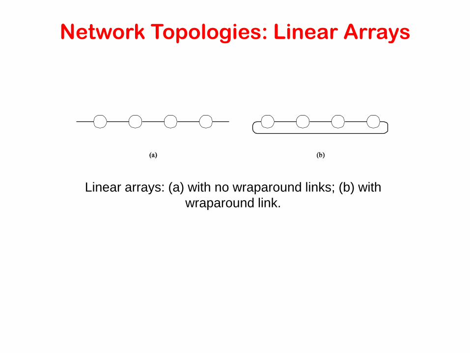
Network Topologies: Linear Arrays

Linear arrays: (a) with no wraparound links; (b) with

wraparound link.

Network Topologies:

Two- and Three Dimensional Meshes

Two and three dimensional meshes: (a) 2-D mesh with no

wraparound; (b) 2-D mesh with wraparound link (2-D torus); and

(c) a 3-D mesh with no wraparound.

Network Topologies:

Hypercubes and their Construction

Construction of hypercubes from hypercubes of lower

dimension.

Network Topologies:

Properties of Hypercubes

• The distance between any two nodes is at most log p.

• Each node has log p neighbors.

• The distance between two nodes is given by the number

of bit positions at which the two nodes differ.

Evaluating

Static Interconnection Networks

• Diameter: The distance between the farthest two nodes in the

network. The diameter of a linear array is p − 1, that of a mesh

is 2( − 1), that of a tree and hypercube is log p, and that of a

completely connected network is O(1).

• Bisection Width: The minimum number of wires you must cut

to divide the network into two equal parts. The bisection width

of a linear array and tree is 1, that of a mesh is , that of a

hypercube is p/2 and that of a completely connected network

is p2/4.

• Cost: The number of links or switches (whichever is

asymptotically higher) is a meaningful measure of the cost.

• Arc Connectivity: is the minimum number of arcs that must

be removed from the network to break it into two disconnected

networks

Evaluating

Static Interconnection Networks

Network Diameter Bisection

Width

Arc

Connectivity

Cost

(No. of links)

Completely-connected

Star

Complete binary tree

Linear array

2-D mesh, no wraparound

2-D wraparound mesh

Hypercube

Wraparound k-ary d-cube

Communication Costs

in Parallel Machines

• Along with idling and contention, communication is a

major overhead in parallel programs.

• The cost of communication is dependent on a variety

of features including the programming model

semantics, the network topology, data handling and

routing, and associated software protocols.

Message Passing Costs in

Parallel Computers

• The total time to transfer a message over a network

comprises of the following:

– Startup time (ts): Time spent at sending and receiving nodes

(executing the routing algorithm, programming routers, etc.).

– Per-hop time (th): This time is a function of number of hops and

includes factors such as switch latencies, network delays, etc.

– Per-word transfer time (tw): This time includes all overheads

that are determined by the length of the message. This

includes bandwidth of links, error checking and correction, etc.

Store-and-Forward Routing

• A message traversing multiple hops is completely

received at an intermediate hop before being

forwarded to the next hop.

• The total communication cost for a message of size m

words to traverse l communication links is

• In most platforms, th is small and the above expression

can be approximated by

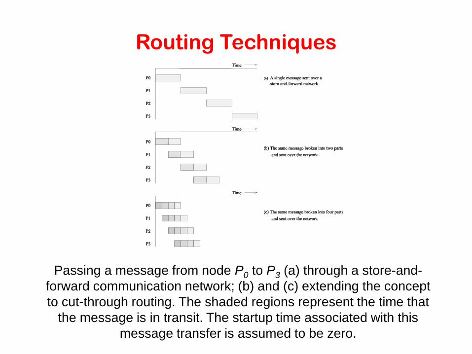
Routing Techniques

Passing a message from node P0 to P3 (a) through a store-and-

forward communication network; (b) and (c) extending the concept

to cut-through routing. The shaded regions represent the time that

the message is in transit. The startup time associated with this

message transfer is assumed to be zero.

Cut-Through Routing

• Takes the concept of packet routing to an extreme by

further dividing messages into basic units called flits.

• Since flits are typically small, the header information

must be minimized.

• This is done by forcing all flits to take the same path, in

sequence.

• A tracer message first programs all intermediate routers.

All flits then take the same route.

• Error checks are performed on the entire message,

as opposed to flits.

• No sequence numbers are needed.

Simplified Cost Model for

Communicating Messages

• The cost of communicating a message between two

nodes l hops away using cut-through routing is given

by

• In this expression, th is typically smaller than ts and

tw. For this reason, the second term in the RHS does

not show, particularly, when m is large.

• Furthermore, it is often not possible to control

routing and placement of tasks.

• For these reasons, we can approximate the cost of

message transfer by

Simplified Cost Model for

Communicating Messages

• It is important to note that the original expression for

communication time is valid for only uncongested

networks.

• If a link takes multiple messages, the corresponding twterm must be scaled up by the number of messages.

• Different communication patterns congest different

networks to varying extents.

• It is important to understand and account for this in the

communication time accordingly.

Routing Mechanisms

for Interconnection Networks

• How does one compute the route that a message takes

from source to destination?

– Routing must prevent deadlocks - for this reason, we use

dimension-ordered or e-cube routing.

– Routing must avoid hot-spots - for this reason, two-step

routing is often used. In this case, a message from source s to

destination d is first sent to a randomly chosen intermediate

processor i and then forwarded to destination d.

Routing Mechanisms

for Interconnection Networks

Routing a message from node Ps (010) to node Pd (111) in a three-

dimensional hypercube using E-cube routing.

Mapping Techniques for Graphs

• Often, we need to embed a known communication

pattern into a given interconnection topology.

• We may have an algorithm designed for one network,

which we are porting to another topology.

For these reasons, it is useful to understand mapping

between graphs.

Mapping Techniques for Graphs: Metrics

• When mapping a graph G(V,E) into G’(V’,E’), the

following metrics are important:

• The maximum number of edges mapped onto any edge

in E’ is called the congestion of the mapping.

• The maximum number of links in E’ that any edge in E is

mapped onto is called the dilation of the mapping.

• The ratio of the number of nodes in the set V’ to that in

set V is called the expansion of the mapping.

Embedding a Linear Array

into a Hypercube

• A linear array (or a ring) composed of 2d nodes (labeled

0 through 2d − 1) can be embedded into a d-dimensional

hypercube by mapping node i of the linear array onto

node

• G(i, d) of the hypercube. The function G(i, x) is defined

as follows:

0

Embedding a Linear Array

into a Hypercube

The function G is called the binary reflected Gray

code (RGC).

Since adjoining entries (G(i, d) and G(i + 1, d)) differ

from each other at only one bit position, corresponding

processors are mapped to neighbors in a hypercube.

Therefore, the congestion, dilation, and expansion of

the mapping are all 1.

Embedding a Linear Array

into a Hypercube: Example

(a) A three-bit reflected Gray code ring; and (b) its embedding into a

three-dimensional hypercube.

Embedding a Mesh

into a Hypercube

• A 2r × 2s wraparound mesh can be mapped to a 2r+s

node hypercube by mapping node (i, j) of the mesh onto

node G(i, r− 1) || G(j, s − 1) of the hypercube (where ||

denotes concatenation of the two Gray codes).

Embedding a Mesh into a Hypercube

(a) A 4 × 4 mesh illustrating the mapping of mesh nodes to the nodes

in a four-dimensional hypercube; and (b) a 2 × 4 mesh embedded into

a three-dimensional hypercube.

Once again, the congestion, dilation, and expansion

of the mapping is 1.

Embedding a Mesh into a Linear Array

• Since a mesh has more edges than a linear array, we

will not have an optimal congestion/dilation mapping.

• We first examine the mapping of a linear array into a

mesh and then invert this mapping.

• This gives us an optimal mapping (in terms of

congestion).

Embedding a Mesh into a Linear Array:

Example

(a) Embedding a 16 node linear array into a 2-D mesh; and (b) the

inverse of the mapping. Solid lines correspond to links in the linear

array and normal lines to links in the mesh.