The candidate confirms that the work submitted is their own and the appropriate credit has been given where reference has been made to the work of others. I understand that failure to attribute material which is obtained from another source may be considered as plagiarism.

(Signature of student)

Automatic Musical Pitch Correction

James Kirkbright

BSc. Computer Science

Session 2003/2004

i

Summary

The purpose of this project was to design and implement an Automatic Pitch Correction System that

is capable of detecting and correcting pitch errors within music. The initial stages of the project

involved research to investigate a range of existing methods currently used for pitch detection and

pitch correction. A system was then designed, based on selected existing algorithms, which is capable

of identifying incorrect notes within an audio sample, determining the pitch that the note should be,

and shifting the pitch of the note by the appropriate amount. The system was implemented within the

MATLAB environment, and operates on both monophonic and polyphonic wav files.

Following the implementation stages, analytical and qualitative evaluation was carried out in order to

assess the system’s performance over a range of different musical input. Analytical evaluation

involved inputting signals of known frequency and observing the performance of both the pitch

detection and the pitch correction within the Automatic Pitch Correction System. Qualitative

evaluation involved the assembly of a group of judges, which enabled user evaluation to be carried

out in order to gain a subjective opinion on the performance of the system.

ii

Acknowledgments

I would like to thank my project supervisor, James Handley for his constant advice and guidance

throughout this project.

Special thanks also goes to those who participated as part of the group of judges during the user

evaluation (see Appendix D).

iii

Table of Contents

1 Introduction ...................................................................................................1

1.1 Problem Definition ...............................................................................................................1 1.2 Project Aim and Objectives..................................................................................................2 1.3 Minimum Requirements .......................................................................................................2 1.4 Possible Extensions ..............................................................................................................3 1.5 Project Schedule ...................................................................................................................3

2 Background Research....................................................................................5

2.1 Introduction ..........................................................................................................................5 2.2 The Fourier Transform .........................................................................................................5 2.3 Pitch Detection .....................................................................................................................6 2.4 Pitch Correction....................................................................................................................8 2.5 Formant Correction ............................................................................................................10

3 Methodology ...............................................................................................12

3.1 Time Domain vs. Frequency Domain................................................................................. 12 3.2 Design Approach ................................................................................................................ 12 3.3 Real-time Considerations ................................................................................................... 13 3.4 Modelling environment ...................................................................................................... 14

4 Design..........................................................................................................15

4.1 Converting to Frequency Domain ...................................................................................... 15 4.2 Pitch Detection ................................................................................................................... 17 4.3 Error Detection ................................................................................................................... 21 4.4 Pitch Correction.................................................................................................................. 24 4.5 Signal Reconstruction......................................................................................................... 28

5 Evaluation ....................................................................................................30

5.1 Evaluation Criteria.............................................................................................................. 30 5.2 Module Performance Results.............................................................................................. 31 5.3 User Evaluation .................................................................................................................. 35

6 Conclusions .................................................................................................39

6.1 Evaluation of Minimum Requirements .............................................................................. 39 6.2 Evaluation of Possible Extensions...................................................................................... 40 6.3 Suggestions for Further Work ............................................................................................ 41

iv

7 Alternative Methods....................................................................................43

7.1 Note Detection.................................................................................................................... 43 7.2 Modified Phase Vocoder .................................................................................................... 44 7.3 Alternative Phase Alignment Techniques .......................................................................... 46

References ...........................................................................................................49

Appendix A .........................................................................................................52

Reflection on Project Experience ..................................................................................................... 52

Appendix B .........................................................................................................53

Project Schedule Gantt Chart ........................................................................................................... 53

Appendix C .........................................................................................................54

External Devices............................................................................................................................... 54

Appendix D .........................................................................................................55

User Evaluation Results.................................................................................................................... 55

1

1 Introduction 1.1 Problem Definition

The standard for modern day musical recordings is higher than ever and the cost of studio time is ever

increasing, often costing in the region of several hundred pounds for a few days recording. Many

hours are wasted in the recording studio, redoing vocal takes or fixing instrument tracks that would

otherwise be perfect except for “that wrong note”. The availability of a system that could

automatically identify and correct imperfect notes could save hours of valuable studio time, avoiding

the frustration caused by constant retakes or the tedious process of correcting pitch errors by hand.

Used to improve the quality of tracks recorded by lesser performer or simply to provide more time to

focus on the creative aspects of recording music, an automatic pitch correction system would be a

valuable addition to any recording studio setup.

Although fixing mistakes in the studio is tedious and time-consuming, it is however possible. Such a

luxury cannot be afforded in live situations. The application of an automatic pitch correction system

that is able to run in real time is required, where wrong notes are detected and corrected in real-time,

as they are being performed. The system would need to output the corrected signal with minimal

delay, accurately correcting any errors in pitch without producing any noticeable coloration or

distortion of the original signal.

The aim of this project is to create a system (note - from here on the system shall be referred to as the

Automatic Pitch Correction System) that will automatically detect and correct the pitch on a single

instrument track without introducing distortion, phase errors, or other artefacts, ideally in real time.

The system shall function for a variety of different recorded instruments and shall aim to produce a

sound signal of the same quality and timbre as the original sound.

The use of computers to present algorithmic solutions to solve problems once only tackled through

traditional analogue circuitry is becoming increasingly important. The number of digital domain

recording and processing tools now available is greater than ever and many applications used within

the musical industry rely upon digital signal processing techniques. The use of computers within the

musical field is therefore highly relevant and such modules as PS23 – Introduction to Scientific

Computing and AR21 – Speech, Audio and Image Processing, provide a basis of knowledge from

which digital signal processing tools such as the Automatic Pitch Correction System may be created.

2

1.2 Project Aim and Objectives

The objectives of the project are to:

• To conduct a thorough investigation into existing methods of pitch detection and pitch

correction and evaluate the possibility of such methods being implemented in real-time.

• To create a system that will accept an audio signal as input, detect any errors in pitch and

correct them accordingly to the nearest note in the chromatic scale, outputting the corrected

signal in real-time.

• The output signal obtained should not only be free from pitch-defects but should maintain the

characteristics and timbre of the original input sound.

• Carry out an evaluation of the system, assessing its performance with respect to its ability to

correct pitch defects, maintain original characteristics of the input sound and output in real-

time.

1.3 Minimum Requirements

The minimum requirements are:

• Discuss current methods and implementations used for detecting and correcting pitch errors

both in real time and in batch processing.

• Create a system that is capable of detecting and correcting pitch errors on a single, simple

instrument track, or tuning fork, without introducing distortion, phase errors, or other

artefacts.

• Evaluate system against current implementations already used for automatic pitch correction.

3

1.4 Possible Extensions

The possible extensions are:

• Perform automatic pitch-correction of input track in real-time, allowing for application in live

performances and real-time monitoring.

• Implement a feature that will allow a specific key to be selected before signal input. This

would enable out of pitch notes to be shifted to the nearest note in the selected key, as

opposed to the nearest note in the chromatic scale.

• The system could possibly be extended to allow pitch-correction of polyphonic material, such

as a de-tuned instrument playing a chord.

1.5 Project Schedule

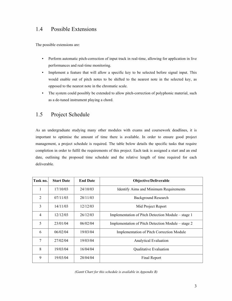
As an undergraduate studying many other modules with exams and coursework deadlines, it is

important to optimise the amount of time there is available. In order to ensure good project

management, a project schedule is required. The table below details the specific tasks that require

completion in order to fulfil the requirements of this project. Each task is assigned a start and an end

date, outlining the proposed time schedule and the relative length of time required for each

deliverable.

Task no. Start Date End Date Objective/Deliverable

1 17/10/03 24/10/03 Identify Aims and Minimum Requirements

2 07/11/03 28/11/03 Background Research

3 14/11/03 12/12/03 Mid Project Report

4 12/12/03 26/12/03 Implementation of Pitch Detection Module – stage 1

5 23/01/04 06/02/04 Implementation of Pitch Detection Module – stage 2

6 06/02/04 19/03/04 Implementation of Pitch Correction Module

7 27/02/04 19/03/04 Analytical Evaluation

8 19/03/04 16/04/04 Qualitative Evaluation

9 19/03/04 28/04/04 Final Report

(Gantt Chart for this schedule is available in Appendix B)

4

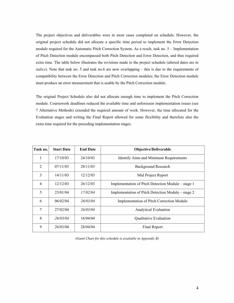
The project objectives and deliverables were in most cases completed on schedule. However, the

original project schedule did not allocate a specific time period to implement the Error Detection

module required for the Automatic Pitch Correction System. As a result, task no. 5 – Implementation

of Pitch Detection module encompassed both Pitch Detection and Error Detection, and thus required

extra time. The table below illustrates the revisions made to the project schedule (altered dates are in

italics). Note that task no. 5 and task no.6 are now overlapping – this is due to the requirements of

compatibility between the Error Detection and Pitch Correction modules; the Error Detection module

must produce an error measurement that is usable by the Pitch Correction module.

The original Project Schedule also did not allocate enough time to implement the Pitch Correction

module. Coursework deadlines reduced the available time and unforeseen implementation issues (see

7 Alternative Methods) extended the required amount of work. However, the time allocated for the

Evaluation stages and writing the Final Report allowed for some flexibility and therefore also the

extra time required for the preceding implementation stages.

Task no. Start Date End Date Objective/Deliverable

1 17/10/03 24/10/03 Identify Aims and Minimum Requirements

2 07/11/03 28/11/03 Background Research

3 14/11/03 12/12/03 Mid Project Report

4 12/12/03 26/12/03 Implementation of Pitch Detection Module – stage 1

5 23/01/04 17/02/04 Implementation of Pitch Detection Module – stage 2

6 06/02/04 26/03/04 Implementation of Pitch Correction Module

7 27/02/04 26/03/04 Analytical Evaluation

8 26/03/04 16/04/04 Qualitative Evaluation

9 26/03/04 28/04/04 Final Report

(Gantt Chart for this schedule is available in Appendix B)

5

2 Background Research

2.1 Introduction

Automatic pitch correction of an audio signal involves the implementation of two separate operations;

pitch detection and pitch correction. Both these operations present many potential problems and

difficulties. Jehan [29] discusses the difficulties associated with detecting the pitch of musically

interesting sounds, since musical sounds are often harmonically rich and have extremely large

frequency ranges. Pitch detection algorithms must be designed to cope with a very large bandwidth,

and must determine pitch during the attack of a note, where amplitude is greatest and harmonic

complexity is at a maximum. Other complications may also arise from the existence of ambiguously

pitched sounds such as multiphonics or un-pitched sounds.

During pitch correction of an audio signal, most problems arise as a result of phase propagation errors

[13]. When performing pitch-modification of a given signal, it is non trivial to alter the frequency at a

given time instant without adversely affecting the phase of the signal too. Algorithms that maintain or

restore phase coherence are required to avoid unwanted defects that are not present in the original

sound. Similarly, harmonics of a signal can be adversely affected by pitch-modification. Formant

information (see 2.5 Formant Correction) particularly can have a significant effect on the nature of a

sound, so it is important that appropriate techniques are employed to preserve formant information

from the original spectrum [28].

2.2 The Fourier Transform

The Fourier Transform [8] may be applied to any sampled signal in order to obtain a representation of

that signal as a group of sinusoidal waves. This allows us to perform complex spectral analysis of the

signal and perform many modifications, such as filtering out certain frequencies, shifting phase, or

even pitch scaling. However, direct evaluation of the Fourier Transform is often extremely

computationally expensive. For this reason, many algorithms exist that allow the Fourier Transform of

a signal to be computed with considerably fewer computations. The set of these algorithms are known

as Fast Fourier Transforms (FFT) [8]. These algorithms work by exploiting the inherent symmetry

present within the expression for the Fourier Transform and contribute significantly to the availability

of real-time signal processing.

6

The Short Time Fourier Transform (STFT) is an important and powerful tool used for spectral

analysis of time-varying signals [8]. When performing spectrum analysis of a time-varying signal,

simply taking the Fourier Transform of the whole signal will not yield useful or meaningful results.

By using a windowing function applied at various time points along the signal, single “frames” of the

signal may be considered to be almost stationary, although the signal is changing over time. Spectral

analysis using the Fourier Transform may then be applied at each of these frames, providing a series

of Fourier Transforms that represent both time-domain and frequency-domain properties of the signal.

2.3 Pitch Detection

Jehan [29] explains the two ways of classifying pitch detection and pitch tracking. The first is

“spectral-domain” based pitch detection, whereby estimations of the time between each change in

pitch (known as pitch period), are obtained by applying a Fourier transform to separate samples of an

input signal. The second is “time-domain” pitch detection, where determination of the Glottal Closure

Instant [5] and measurement of the time period between “events” within the input signal allow

estimation of the pitch period. However, the latter approach is often not suited to music input signals

due to the inherently wide range of fundamental frequencies present.

Godsill et al. [27] discuss a spectral domain based method that is used to detect deviation of pitch over

a long-time scale. This method is employed in the “smoothing” of audio signals that contain defects

such as “wow” or “flutter” (time-varying pitch defects not present in the original recording), common

in many old musical recordings. The method works by using “frequency tracking”, a process whereby

the input data is converted into a time frequency “map” that can be used to detect the pitch of

principle frequency components. Once this stage is complete, pitch variations can be analysed and any

variations that affect all tones present within the music may be attributed to the defects caused by

“wow” or “flutter”. Other variations present may be attributed to genuine note changes or

progressions within the music and therefore can be ignored.

The frequency tracking uses the discrete Fourier Transform [8] to estimate as many tonal frequency

components present within the data as possible. When sampling the input audio, window lengths are

chosen to be short enough such that the signal within a single block is almost constant, and therefore

non-time-varying. This then allows blocks of data sharing similar frequency and amplitude to be

placed together along the same “frequency track”. The evolution of these frequency tracks may then

be used to estimate a pitch variation curve and then through subsequent processing, the defects may

be removed (see 2.4 Pitch Correction).

7

Jehan [29] proposes a multi-resolution, multi-scale analysis approach to pitch detection using

mathematical functions known as “wavelets” [11]. Wavelets work by separating data into different

frequency components and then applying a windowing length appropriate to the present frequency.

For example, long window lengths are used at low frequencies, whilst short window lengths are used

at high frequencies. This approach is advantageous over traditional Fourier methods since input

signals may contain such features as sharp peaks that require analysis at a greater resolution. It is

considered desirable to perform analysis in this way since human hearing works in a similar way [29].

Noll [1] introduces a frequency domain based pitch determination technique that may be used for

human speech known as the Harmonic Product Spectrum (HPS). The algorithm works by analysing

the short-term frequency content of a signal obtained using the STFT. The algorithm is

computationally efficient and is capable of running in real-time [21]. HPS works on the theory that the

spectrum of a musical note consists of a series of peaks, where one peak corresponds to the

fundamental frequency and all remaining peaks correspond to harmonic components at integer

multiples of the fundamental frequency. To obtain the fundamental frequency, the spectrum is

compressed multiple times by an integer factor and compared against the original unaltered spectrum.

Multiplying the spectrums together produces strong peaks where harmonics line up, where the largest

of these peaks created represents the fundamental frequency.

There are two main drawbacks to the Harmonic Product Spectrum algorithm. Firstly, the accuracy of

the calculated fundamental frequency depends on the size of the Fourier transform used; a larger

Fourier transform corresponds to a larger number of frequency bins and therefore a higher accuracy in

identifying the fundamental frequency, whilst a smaller Fourier Transform corresponds to a smaller

number of frequency bins and therefore reduced accuracy; if the fundamental frequency of the input

signal falls between two frequency bins, the frequency has to be approximated. The second problem

occurs when multiplying spectrums together results in more than one major harmonic peak in the

power spectrum [20]. This almost always results in detecting the fundamental frequency one octave

too high [21]. The latter problem may be overcome by performing a post-processing algorithm

whereby amplitude peaks in the power spectrum are compared and if a lower peak exists that is of

sufficiently large amplitude then the lower octave peak is selected as the fundamental frequency.

A popular time-domain based solution for pitch detection is to use the Autocorrelation function [9, 17,

22]. The autocorrelation function is defined as the sum of absolute differences between points along

two different signals over a given interval. To detect the fundamental frequency of a signal, windowed

samples are taken that correspond to at least twice as long as the longest period to be detected. For

each windowed sample, a copy of the signal is shifted and compared with the original. Since all

periodic signals remain similar from one period to the next, as the shift amount approaches the

8

fundamental period of the windowed signal, the pointwise difference between the two signals will

decrease and therefore so will the autocorrelation function. To calculate the fundamental frequency

therefore requires finding the first minimum within the autocorrelation function, which corresponds to

the fundamental period of the signal, from which the fundamental frequency may be calculated. This

value may be detected by differentiating the autocorrelation function to find regions where polarity is

reversed from negative to positive, thus corresponding to a minimum.

Although the above method is robust to noise and is capable of accurate results, using the

autocorrelation function to detect fundamental frequency is computationally expensive and requires a

high sampling rate in order to achieve high-resolution pitch detection. A lower sampling rate restricts

the amount by which signals may be shifted for comparison and therefore limits the resolution of

frequencies that may be detected.

2.4 Pitch Correction

There exist two fundamental methods for altering the pitch of a signal [28]. The first is “Frequency

Shifting”, a process whereby the input signal is shifted in frequency by modulating an analytical

signal by a complex exponential. However, this tends to lead to unwanted distortion of the original

sound signal, creating a metallic, inharmonic sound, non-comparable to the input signal. The second

method is to use “Time/Pitch Scaling”, where altering the length of a sound and then applying some

sample rate conversion technique to change the frequency achieve a change in pitch whilst preserving

the harmonic qualities of the input signal.

Bernsee [28] introduces a popular technique used for time/pitch scaling, known as Time Domain

Harmonic Scaling (TDHS). Based on a method proposed by Rabiner and Schafer [18], TDHS works

by estimating the basic pitch period [27, 18] of the input signal. The fundamental frequency is then

calculated using the Short Time Average Magnitude Difference [18]. An output signal can then be

created by copying the input signal in an “overlap-and-add” fashion, whilst simultaneously

incrementing the input pointer relative to the fundamental frequency. This method of “Synchronised

Overlap and Add” results in the input signal being traversed at a different speed, thus creating a

change in pitch. Then by using the pitch period estimate, the signal may be aligned such that the time

base is unchanged, resulting in a pitch corrected signal of unchanged length.

However, time domain based techniques such as TDHS are often unsuited to polyphonic material and

suffer from high complexity due to the fact that estimation of fundamental frequency is required

before pitch scaling may be performed. To overcome these drawbacks, time/pitch scaling may be

9

performed in the frequency domain, where no estimation of fundamental frequency is required at all,

resulting in lower complexity and fewer calculations than those performed in the time domain. [16]

The Phase Vocoder [4, 14, 15, 16, 18] is a well-established frequency domain method used for

time/pitch scaling of audio signals. The Phase Vocoder is an algorithm that allows either the timescale

or pitch of a signal to be modified, without adversely affecting the other. For example, timescale

modification on a signal may be performed without altering pitch, or pitch modification may be

performed whilst retaining the original time base of the signal.

Phase Vocoder based techniques accomplish pitch modification by a sequence of analysis,

modification and re-synthesis. During analysis, an STFT is applied to the input signal. The calculation

obtained at each time point within the STFT corresponds to a vocoder “channel”. Following this,

individual channels may then be altered accordingly to create the desired pitch-modification. Re-

synthesis is then performed using the Inverse Fast Fourier Transform [8]. The Phase Vocoder is

considered a powerful tool, due mainly to its efficient implementation using the Fast Fourier

Transform (FFT) [14].

Laroche et al [14] explain that pitch scaling is achieved using the Phase Vocoder by altering the time

base of an input signal, thus creating a change in pitch. The signal is then resampled at an appropriate

sampling rate in order to restore the original replay rate of the signal whilst maintaining the change in

pitch. An important drawback of this scheme, highlighted by Laroche et al [14] is that only linear

frequency-alterations may be made to the input signal. To overcome this lack of flexibility and the

restrictions it imposes, Laroche et al [14] introduce two alternative implementations of the phase

vocoder, both aiming to improve flexibility by using a two-stage system of peak detection and peak

translation to achieve a change in frequency. A subsequent phase-adjustment is then required to avoid

phasing errors and maintain phase coherence between frames. Since each peak may be “shifted”

individually, non-linear frequency modifications may be obtained.

Garas et al [16] suggest an improved implementation of the phase vocoder inspired by the human

auditory system, where spectral analysis is performed in a non-uniform manner, thus simulating the

non-uniform way in which humans decode audio signals. To achieve this, a warping function is

applied to modify the spectral resolution produced by the use of the Fast Fourier Transform [4, 8, 18,

19]. The modification is made so that the constant-bandwidth resolution becomes a constant-Q

resolution, otherwise known as a percentage bandwidth. For example, resolution is decreased at lower

frequency and is increased at higher frequencies. This method of percentage bandwidth spectral

analysis is similar to the multi-resolution, multi-scale pitch detection algorithm discussed by Jehan

[29] (see 4.2 Pitch Detection).

10

This concept of a “constant-Q phase vocoder” overcomes the issue of lower signal quality resulting

from working in the frequency domain, whilst still maintaining relatively low complexity, comparable

to the implementation of the traditional phase vocoder.

The phase vocoder does however have its drawbacks. Laroche et al. [13] discuss how, without proper

pre-processing, unwanted artefacts such as “transient smearing” and “phase incoherence” can occur in

the output signal. Transient smearing manifests itself as a reduction in the percussive nature of a

signal - notes lose their “attack”, whilst phase incoherence results in a loss of “presence” in the output

signal. For example, a vocalist or solo instrument may appear to be further away from the microphone

than in the original recording.

Use of the STFT is widely considered to be the underlying reason for phase propagation errors such as

transient smearing and phase incoherence [13]. This is due to the fact that although the STFT ensures

phase consistency within each channel over time, but does not however ensure phase consistency

across all channels (known as vertical phase coherence). Although this problem may be avoided by

only using integer modifications factors, the use of non-integer modification factors can often lead to

significant defects within the output signal. Laroche et al. [13] explain how the application of a

“Phase-Locked Phase Vocoder” may help to eliminate phase incoherence, thus creating a more

desirable output signal. The vocoder works by using a peak detection algorithm to detect peak

channels within the input signal, then by only allowing the phase of peak channels to be updated, the

phase of all other channels may be “locked”, therefore maintaining vertical phase coherence across

channels.

2.5 Formant Correction

Whenever pitch-modification of an audio signal is performed, not only is the pitch of the signal

changed, but formants present within the signal are moved as well [28]. Since the position and

frequency of formants very much determine the character and nature of a sound, it is important to

apply some formant-correction or formant-preservation technique in order to achieve desirable results.

Bernsee [28] explains how formant-correction may be achieved when using the phase vocoder. The

technique works by removing any newly generated formants within the output signal and

superimposing the original formant information from the input signal. This is achieved by

normalizing the spectral amplitude envelope of the output signal and multiplying it by the original

non-pitch scaled version. Since this is an amplitude-only frequency domain based method, the

additional computational costs involved are minimal.

11

Laroche [15] proposes a similar method, whereby pitch and formant modification are performed

simultaneously. The method is primarily designed to work on monophonic sound sources, achieving

results comparable with that of time-domain based methods, whilst maintaining the flexibility of

working in the frequency domain. Pitch correction is performed by translating peaks within the signal

to a new “target frequency” then rotating the phases of peaks and (surrounding bins) by an amount

relative to the phase-increment as a result of the change in pitch. The formant correction is

implemented by locating individual harmonics within the original spectrum. Selected harmonic

regions with frequency closest to that of the output harmonic are then pasted into the output signal at

the desired frequency, thus preserving the original formant information.

Within the time domain, pitch and formant information may be manipulated independently. Bernsee

[28] discusses a formant-preservation technique where Time Domain Harmonic Scaling is

implemented as a granular synthesis, where grains of length equivalent to one cycle of the

fundamental frequency are output at a new destination frequency rate. Pitch modification is then

achieved simply by altering the output rate of grains, whilst discarding some grains in the process to

maintain the length of the original sample. Since no transposition actually takes place during this

process, formants are not moved.

12

3 Methodology 3.1 Time Domain vs. Frequency Domain

The first decision to be made regarding the proposed design methodology to be used for the

Automatic Pitch Correction System involved comparison between time domain and frequency domain

based techniques. As previously discussed (see 2 Background Research), frequency domain based

techniques for both Pitch Detection and Pitch Correction are more computationally efficient than time

domain based techniques. Time domain based techniques such as the autocorrelation function (used

for pitch detection) and Time Domain Harmonic Scaling (used for pitch correction) both suffer from

large computational expense whilst their frequency domain counterparts, such as Harmonic Product

Spectrum, and the Phase Vocoder require fewer calculations and are more computationally efficient.

For this reason, the Automatic Pitch Correction system implements both pitch detection and pitch

correction in the frequency domain.

3.2 Design Approach

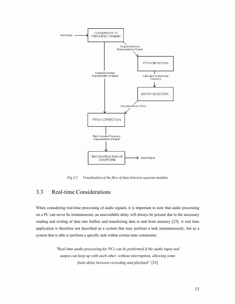
The Automatic Pitch Correction System requires three separate operations to perform automatic

correction: Pitch Detection, Error Detection and Pitch Correction. For this reason it was decided that a

pipeline process model should be used where each of these stages is implemented as a separate

“stand-alone” module. Two more modules that dealt with the conversion between time domain and

frequency domain were also used in order to maintain the modular construction of the system

throughout. Thus the resulting pipeline involves five separate processes: Conversion to Frequency

Domain, Pitch Detection, Error Detection, Pitch Correction and Reconstruction of the Waveform.

Implementation as a modular system offers greater flexibility and allows for improvements and

modifications to be made to each module individually without affecting other modules present within

the system. For example, the use of different Pitch Detection process would not require any changes

to be made to the Error Detection and Pitch Correction modules.

Fig 3.2 demonstrates the interaction between the separate modules, detailing the flow of data and

information required by each module. The system architecture is designed in a linear fashion, without

the need for feedback or recursive loops.

13

Fig 3.2 Visualisation of the flow of data between separate modules

3.3 Real-time Considerations

When considering real-time processing of audio signals, it is important to note that audio processing

on a PC can never be instantaneous; an unavoidable delay will always be present due to the necessary

reading and writing of data into buffers and transferring data to and from memory [23]. A real time

application is therefore not described as a system that may perform a task instantaneously, but as a

system that is able to perform a specific task within certain time constraints:

"Real-time audio processing for PCs can be performed if the audio input and

output can keep up with each other, without interruption, allowing some

finite delay between recording and playback” [23]

14

In terms of signal processing, a real-time process should in theory be executed “on the fly” and

therefore regarded as a sequential process, whereby the signal input is split up into consecutive

discrete sections that may be operated on individually, in a sequential fashion. Each section is

operated on separately and therefore processing of a single section should be completed before the

following section is reached.

3.4 Modelling environment

The choice of developing environment for the Automatic Pitch Correction System is of significant

importance and may greatly affect the potential capabilities of the resulting software. A number of

different options are available such as C, Java, Maple or MATLAB. MATLAB is a comprehensive

programming development environment with a large library of existing functions and therefore highly

suited to the task of developing the Automatic Pitch Correction System. The decision to use

MATLAB was influenced by several key features:

• Large library of useful existing functions

• Scripts and programs can be created without the need for compilation

• Interactive displays and debugging capabilities

• Array based computation allows for very fast processing times

• MATLAB scripts may be embedded in C code, allowing for further development as a

real-time application

The Automatic Pitch Correction system is implemented as a frequency domain based system, and

therefore requires Fourier representation of audio signals. MATLAB allows for multiple file formats

to be read or written, including WAV files and is therefore highly suitable for manipulating audio

data. MATLAB has built in functions for the Fast Fourier Transform and the Inverse Fourier

Transform, and therefore simplifying the task of converting between time domain and frequency

domain. There are also many functions available within MATLAB’s existing libraries that are able to

operate on complex numbers and functions are provided that allow manipulation of real and

imaginary parts of complex numbers separately – an important consideration when manipulating

phase angles of an audio signal in its frequency domain representation

15

4 Design

4.1 Converting to Frequency Domain

The first stage is to convert the signal waveform from the time-domain to the frequency domain. This

is done using the Short Time Fourier Transform [8]. The sampling rate sr of the input signal, and the

desired length (in ms) of each window w determine the size of each Fourier Transform:

The Short Time Fourier Transform returns a series of overlapping short-term Fast Fourier Transform

(FFT) frames, each one corresponding to an analysis window within the input signal. The reason for

choosing to overlap successive FFT frames is twofold: Firstly, the process of overlapping helps to

create a cross-fade effect between frames, giving a smoother transition when re-assembling the

spectrogram back to a waveform. Secondly, a greater number of frames may be retrieved over a given

time period, which, as will be discussed later, allows for greater resolution during the pitch shifting

process (see 4.4 Pitch Correction).

The choice of windowing function used is important when performing a Fourier transform and can

have a significant affect on the accuracy of the results that may be obtained [25]. The windowing

function used throughout the Automatic Pitch Correction System is the Hanning function. Using a

Hanning window allows for a 75% overlap, which allows a greater number of FFTs to be calculated

over a shorter section of signal. This is desirable since the resolution of the Pitch correction used

depends on the number of FFT frames calculated (see 4.4 Pitch correction). The more frames used,

the greater the resolution of the pitch shifting and for real-time application, these FFT frames need to

be calculated in as short a time as possible. The Hanning window also prevents leakage, or smearing

between frequencies where successive frames overlap [25] and therefore offers superior frequency

representation, thus increasing the potential accuracy of the pitch detection that will follow.

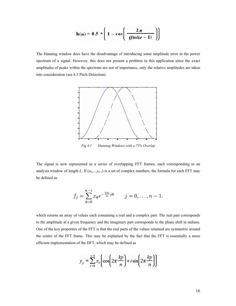
The Hanning function h(n) is applied to each analysis window, allowing for a 75% overlap between

each fft frame (see Fig 4.1). The function is applied to all points in each analysis window ( n =

1,…,ftsize ) and is defined as

16

The Hanning window does have the disadvantage of introducing some amplitude error in the power

spectrum of a signal. However, this does not present a problem in this application since the exact

amplitudes of peaks within the spectrum are not of importance, only the relative amplitudes are taken

into consideration (see 4.3 Pitch Detection).

Fig 4.1 Hanning Windows with a 75% Overlap

The signal is now represented as a series of overlapping FFT frames, each corresponding to an

analysis window of length L. If (x0,...,xn-1) is a set of complex numbers, the formula for each FFT may

be defined as

which returns an array of values each containing a real and a complex part. The real part corresponds

to the amplitude at a given frequency and the imaginary part corresponds to the phase shift in radians.

One of the key properties of the FFT is that the real parts of the values returned are symmetric around

the centre of the FFT frame. This may be explained by the fact that the FFT is essentially a more

efficient implementation of the DFT, which may be defined as

17

and since the real part returned by the DFT is essentially the cos function and the complex part is the

sin, the real parts of the FFT values must be symmetrical. For this reason, efficiency is improved in

the Automatic Pitch Correction System by only calculating and storing the first (ftsize/2) values

returned by the FFT for each analysis window.

As discussed previously, in order to achieve non-linear frequency alterations, it is required that the

input signal is divided into separate sections of finite length, each of which may be manipulated

individually. To make this possible, the corresponding spectrogram representation of the signal must

be separated into sections, each containing an equal number of FFT frames. Since individual FFT

frames are overlapping, the separate sections must also overlap. Given a 75% overlap, the hop size

between two successive frames is equal to ftsize/4 whilst the actual overlapping region is equal to

3*ftsize/4. Therefore, given two separate sections of contiguous FFT frames, the overlapping region

will consist of three frames from each section (see Fig 4.10). This frame overlap is important in

ensuring a smooth transition between successive sections upon reconstruction of the output signal.

However, overlaps consisting of modified sections require special treatment since the waveform

characteristics have been altered and therefore phase re-alignment will need to be performed. This

will be discussed in a later chapter (see 4.4 Pitch Correction).

4.2 Pitch Detection

Pitch detection in the Automatic Pitch Correction System is implemented as a frequency domain

based technique. Based on the Harmonic Product Spectrum [1], the algorithm requires analysis of the

power spectrum of the input signal, whereby the magnitude and position of peaks detected within the

spectrum are used to determine the fundamental frequency. However, unlike the Harmonic Product

Spectrum, where the power spectrum is multiplied and downsampled multiple times, the algorithm

used in the Automatic Pitch Correction System is capable of returning the same results but without the

multiplication/downsampling stages and therefore is more computationally efficient.

Firstly, the input signal is sampled using a fixed window size. A Hanning window function is applied

to each window and the fast Fourier transform is applied across all points in the windowed sample in

order to obtain the power spectrum.

18

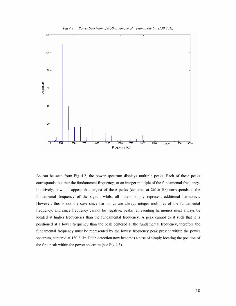
Fig 4.2 Power Spectrum of a 50ms sample of a piano note C3 (130.8 Hz)

As can be seen from Fig 4.2, the power spectrum displays multiple peaks. Each of these peaks

corresponds to either the fundamental frequency, or an integer multiple of the fundamental frequency.

Intuitively, it would appear that largest of these peaks (centered at 261.6 Hz) corresponds to the

fundamental frequency of the signal, whilst all others simply represent additional harmonics.

However, this is not the case since harmonics are always integer multiples of the fundamental

frequency, and since frequency cannot be negative, peaks representing harmonics must always be

located at higher frequencies than the fundamental frequency. A peak cannot exist such that it is

positioned at a lower frequency than the peak centered at the fundamental frequency, therefore the

fundamental frequency must be represented by the lowest frequency peak present within the power

spectrum, centered at 130.8 Hz. Pitch detection now becomes a case of simply locating the position of

the first peak within the power spectrum (see Fig 4.3).

19

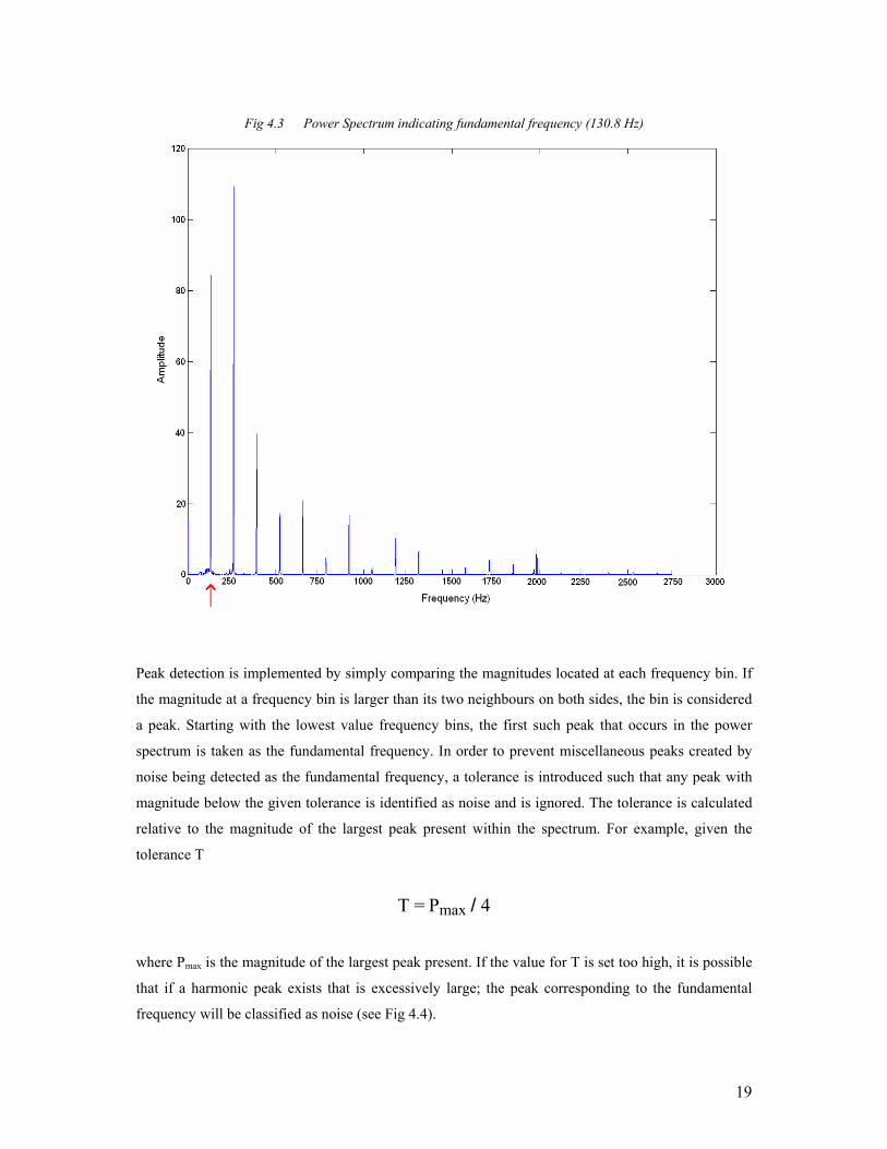
Fig 4.3 Power Spectrum indicating fundamental frequency (130.8 Hz)

Peak detection is implemented by simply comparing the magnitudes located at each frequency bin. If

the magnitude at a frequency bin is larger than its two neighbours on both sides, the bin is considered

a peak. Starting with the lowest value frequency bins, the first such peak that occurs in the power

spectrum is taken as the fundamental frequency. In order to prevent miscellaneous peaks created by

noise being detected as the fundamental frequency, a tolerance is introduced such that any peak with

magnitude below the given tolerance is identified as noise and is ignored. The tolerance is calculated

relative to the magnitude of the largest peak present within the spectrum. For example, given the

tolerance T

T = Pmax / 4

where Pmax is the magnitude of the largest peak present. If the value for T is set too high, it is possible

that if a harmonic peak exists that is excessively large; the peak corresponding to the fundamental

frequency will be classified as noise (see Fig 4.4).

20

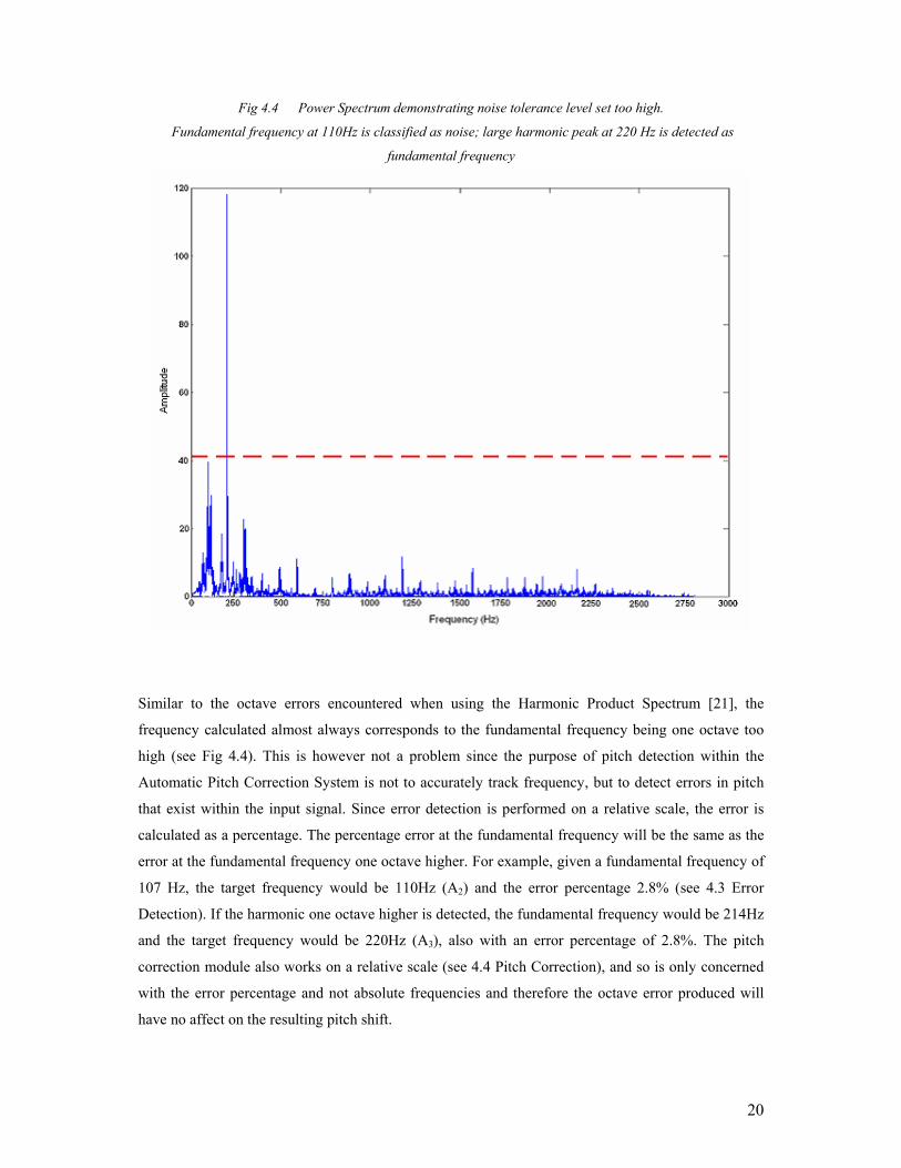
Fig 4.4 Power Spectrum demonstrating noise tolerance level set too high.

Fundamental frequency at 110Hz is classified as noise; large harmonic peak at 220 Hz is detected as

fundamental frequency

Similar to the octave errors encountered when using the Harmonic Product Spectrum [21], the

frequency calculated almost always corresponds to the fundamental frequency being one octave too

high (see Fig 4.4). This is however not a problem since the purpose of pitch detection within the

Automatic Pitch Correction System is not to accurately track frequency, but to detect errors in pitch

that exist within the input signal. Since error detection is performed on a relative scale, the error is

calculated as a percentage. The percentage error at the fundamental frequency will be the same as the

error at the fundamental frequency one octave higher. For example, given a fundamental frequency of

107 Hz, the target frequency would be 110Hz (A2) and the error percentage 2.8% (see 4.3 Error

Detection). If the harmonic one octave higher is detected, the fundamental frequency would be 214Hz

and the target frequency would be 220Hz (A3), also with an error percentage of 2.8%. The pitch

correction module also works on a relative scale (see 4.4 Pitch Correction), and so is only concerned

with the error percentage and not absolute frequencies and therefore the octave error produced will

have no affect on the resulting pitch shift.

21

Performing Pitch detection in this way has both its advantages and its disadvantages. Firstly, the

technique is computationally very efficient, requiring fewer computations than the Harmonic Product

Spectrum, which is capable of running in real time [21]. The algorithm is reasonably robust to noise

and works for a variety of different inputs. The disadvantage of using any technique that uses the

power spectrum to determine fundamental frequency is that resolution is dependent on the length of

the FFT used. A short and fast FFT results in a limited number of frequency bins and therefore a

lower resolution in pitch determination. For a greater number of frequency bins and therefore a higher

resolution, a longer window must be used to calculate the FFT, which requires a greater amount of

time.

4.3 Error Detection

4.3.1 Pitch Perception and Frequency of Musical Notes

In order to implement error detection correctly, it is important to understand the difference between

pitch and frequency. ‘Pitch’ is a description of the subjective sound of a signal whilst frequency is an

actual representation of the sound’s physical structure. The difference between pitch and frequency is

demonstrated by the fact that polyphonic sounds involving more than one frequency are often

perceived as a single pitch [2].

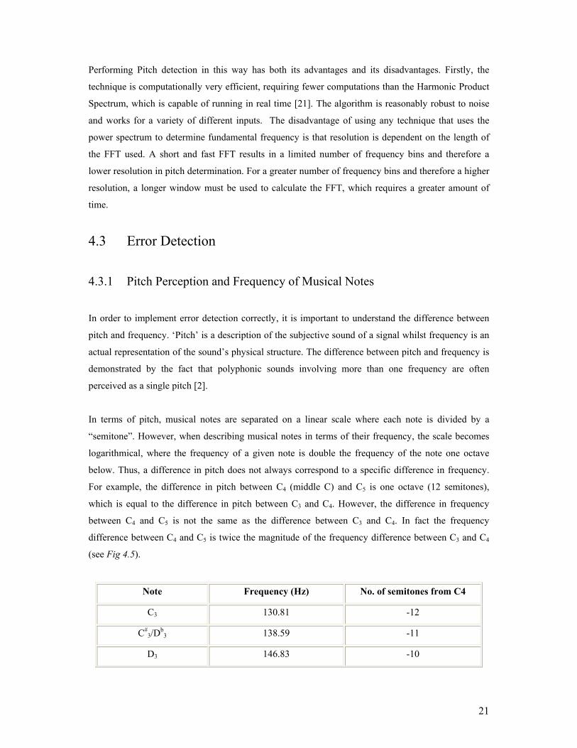
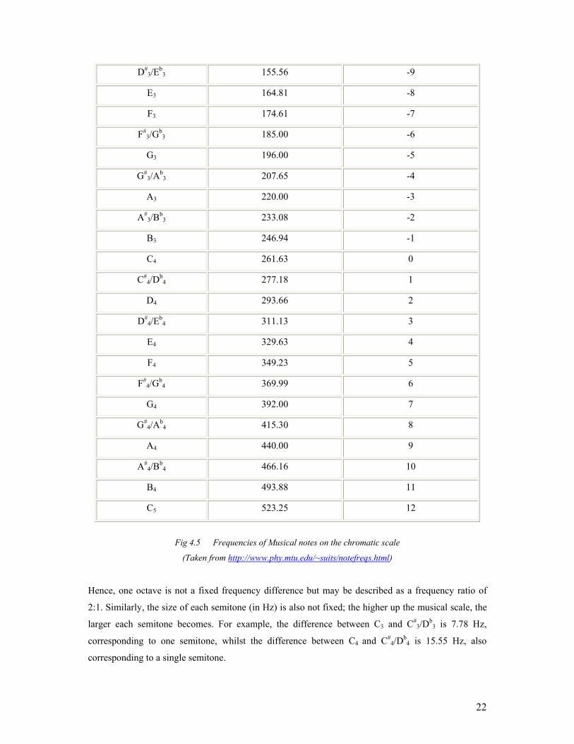
In terms of pitch, musical notes are separated on a linear scale where each note is divided by a

“semitone”. However, when describing musical notes in terms of their frequency, the scale becomes

logarithmical, where the frequency of a given note is double the frequency of the note one octave

below. Thus, a difference in pitch does not always correspond to a specific difference in frequency.

For example, the difference in pitch between C4 (middle C) and C5 is one octave (12 semitones),

which is equal to the difference in pitch between C3 and C4. However, the difference in frequency

between C4 and C5 is not the same as the difference between C3 and C4. In fact the frequency

difference between C4 and C5 is twice the magnitude of the frequency difference between C3 and C4

(see Fig 4.5).

Note Frequency (Hz) No. of semitones from C4

C3 130.81 -12

C#3/Db

3 138.59 -11

D3 146.83 -10

22

D#3/Eb

3 155.56 -9

E3 164.81 -8

F3 174.61 -7

F#3/Gb

3 185.00 -6

G3 196.00 -5

G#3/Ab

3 207.65 -4

A3 220.00 -3

A#3/Bb

3 233.08 -2

B3 246.94 -1

C4 261.63 0

C#4/Db

4 277.18 1

D4 293.66 2

D#4/Eb

4 311.13 3

E4 329.63 4

F4 349.23 5

F#4/Gb

4 369.99 6

G4 392.00 7

G#4/Ab

4 415.30 8

A4 440.00 9

A#4/Bb

4 466.16 10

B4 493.88 11

C5 523.25 12

Fig 4.5 Frequencies of Musical notes on the chromatic scale

(Taken from http://www.phy.mtu.edu/~suits/notefreqs.html)

Hence, one octave is not a fixed frequency difference but may be described as a frequency ratio of

2:1. Similarly, the size of each semitone (in Hz) is also not fixed; the higher up the musical scale, the

larger each semitone becomes. For example, the difference between C3 and C#3/Db

3 is 7.78 Hz,

corresponding to one semitone, whilst the difference between C4 and C#4/Db

4 is 15.55 Hz, also

corresponding to a single semitone.

23

Since higher pitched notes are separated by a greater amount on the frequency scale than lower notes,

frequency resolution is also increased as notes move up the musical scale. This is even demonstrated

in human hearing. A human is far more capable of discerning pitch at higher frequencies since a

difference in pitch corresponds to a larger difference in frequency and therefore is more recognizable

to the human ear.

4.3.2 Implementation

Since pitch correction in the Automatic Pitch Correction System is implemented to shift pitch on a

relative scale, error detection in the Automatic Pitch Correction System is also implemented on a

relative scale. The difference between the detected note and the calculated “target note” is returned as

an error percentage. As discussed earlier, higher musical notes are separated by larger frequencies

than those lower down in the musical scale and therefore the frequency resolution will be higher for

higher frequencies, and lower for lower frequencies.

Error detection is implemented by storing an array in memory containing the frequency values for C0

to B1. Multiplying each of these vales by 2 multiple times then creates a lookup table containing

frequency values for C0 to C5. For each windowed sample, the calculated frequency of the input signal

is compared with the values stored in the lookup table. The “target note” for the windowed sample is

calculated using a “nearest neighbour” approach implemented in Matlab using the DSEARCH

function, which uses an algorithm known as Delaunay triangulation [6]. The closest match (i.e.

nearest neighbour) contained within the lookup table is returned as the target note/frequency. Given

the target frequency, the error percentage is then calculated as

e = 100 * (T – f) / f

where e is the relative percentage error, T is the target frequency (in Hz) and f is the calculated

frequency (in Hz) of the windowed sample. The error e corresponds to the relative increase/decrease

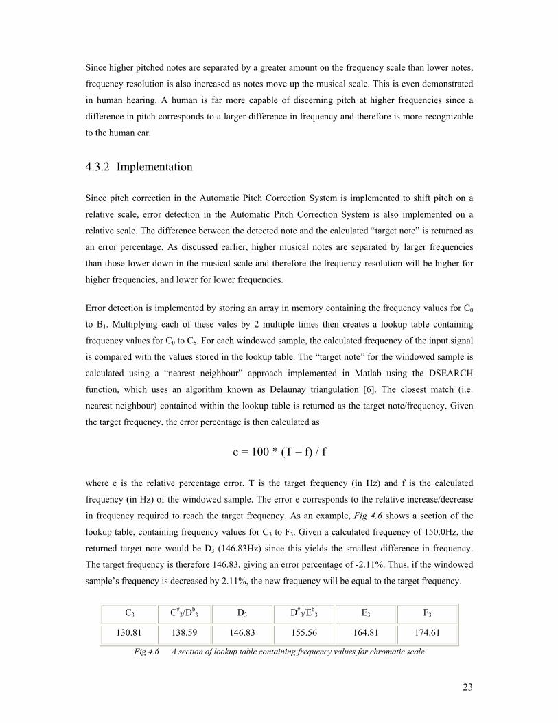
in frequency required to reach the target frequency. As an example, Fig 4.6 shows a section of the

lookup table, containing frequency values for C3 to F3. Given a calculated frequency of 150.0Hz, the

returned target note would be D3 (146.83Hz) since this yields the smallest difference in frequency.

The target frequency is therefore 146.83, giving an error percentage of -2.11%. Thus, if the windowed

sample’s frequency is decreased by 2.11%, the new frequency will be equal to the target frequency.

C3 C#3/Db

3 D3 D#3/Eb

3 E3 F3

130.81 138.59 146.83 155.56 164.81 174.61

Fig 4.6 A section of lookup table containing frequency values for chromatic scale

24

4.4 Pitch Correction

4.4.1 Underlying Idea

The underlying technique used to obtain a pitch shift in the Automatic Pitch Correction System is

based on the Phase Vocoder. The Phase Vocoder is a high quality frequency domain solution to pitch

alteration that works equally well for both monophonic and polyphonic material and therefore is well

suited for the purposes of the Automatic Pitch Correction System. The Phase Vocoder does however

have its drawbacks; the most important is that in its standard form it is fundamentally only capable of

linear frequency alterations [14]. To explain this, the standard technique obtains a shift in pitch by

first modifying the time base of the signal and then altering the sampling rate of playback (i.e.

resampling) to effect a pitch change and restore the signal to its original length. Since the resampling

stage cannot be implemented until the entire signal has been processed, any shift in pitch that is

created applies to the entire signal and therefore non-linear frequency alterations are not possible.

For the Automatic Pitch Correction System, a modified implementation of the Phase Vocoder is used,

where sequential processing is used to solve the problem of non-linear frequency alterations. As the

input signal is being read, it is separated into multiple smaller discrete sections and the time-

scale/resample Phase Vocoder technique is applied to each section individually. The implementation

of the resampling stage differs from that used in the standard Phase Vocoder in that instead of actually

playing the signal back at a different sampling rate, the waveform itself is modified using

interpolation to restore the signal back to its original time base. This form of “resampling” allows

each section to be played back at the same sampling rate, regardless of the pitch shift required.

The final stage involves the construction of the output array, produced through reconstruction of the

separate sections. The sections are joined back together and played back at the same sampling rate as

the input signal. Those sections that have been modified by the time-scale/resample operation will

play back at the same speed as in the input signal, but at a different pitch whilst all other sections will

remain unchanged. This reconstruction stage may also be considered as a sequential process since it is

possible to add each section to the output array as soon as it has been processed. Therefore, given that

small enough section lengths are chosen, possibilities are created for the pitch shifting process to be

implemented as a real-time application.

25

4.4.2 Time Scaling

Time scaling of each section of the signal is implemented in the frequency domain. As discussed in

the previous section, the STFT returns a series of FFT frames, each corresponding to an analysis

window within the input signal. The number of frames N therefore corresponds to the length (i.e. the

time base) of the signal. Given an FFT size ftsize a window hop size hop and a sampling rate sr

L = ( ftsize + ( (N –1) * hop ) ) * (1000/sr)

where N represents the number of FFT frames present and L represents the length (in ms) of the

corresponding output signal. Therefore, in order to alter the time base of a signal, the number of

frames N must be altered. This is achieved by interpolating between successive FFT frames, thus

introducing or removing frames such that the new value for N corresponds to the new time base. The

modification to the time base may therefore be calculated simply as the number of FFT frames to be

added or removed. Given that the pitch of a section of signal is to be scaled by a factor β, the change

in number of FFT frames ∆N may be calculated as

∆N = ( β * N ) – N

It is important to note that only an integer number of FFT frames may be added or removed and

therefore the degree to which pitch may be shifted is dependent upon the size of N. For example, to

effect a 1% increase in pitch (i.e. β = 1.01), it is required that N ≥ 100. The resolution of pitch shift is

therefore a function of the size of N, where a larger size of N results in higher resolution pitch shifting.

In fact, the minimum frequency alteration fmin (% relative to original frequency) may be described as

The choice of N is therefore an important aspect of the Automatic Pitch Correction system. Although

a larger N corresponds to a higher frequency resolution, it also results in a lower time resolution.

Similarly, a smaller N corresponds to a higher time resolution but with a lower frequency resolution.

26

Each FFT frame yields an array of complex values of the form

X(Ω, t) = H(Ω) exp jφ

where H(Ω) represents the Fourier transform of the analysis window h(n) at time t corresponding to

the frequency Ω. For each FFT frame, the real part of X(Ω, t) represents the magnitude spectrum of

the FFT, whilst the complex part represents the phase angle information denoted by φ. To perform

interpolation between FFT frames, the real and complex parts of the FFT values must be interpolated

separately.

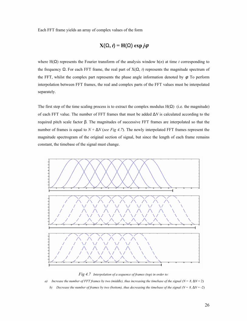
The first step of the time scaling process is to extract the complex modulus H(Ω) (i.e. the magnitude)

of each FFT value. The number of FFT frames that must be added ∆N is calculated according to the

required pitch scale factor β. The magnitudes of successive FFT frames are interpolated so that the

number of frames is equal to N + ∆N (see Fig 4.7). The newly interpolated FFT frames represent the

magnitude spectrogram of the original section of signal, but since the length of each frame remains

constant, the timebase of the signal must change.

Fig 4.7 Interpolation of a sequence of frames (top) in order to:

a) Increase the number of FFT frames by two (middle), thus increasing the timebase of the signal (N = 8, ∆N = 2)

b) Decrease the number of frames by two (bottom), thus decreasing the timebase of the signal (N = 8, ∆N = -2)

27

4.4.3 Phase Alignment

Phase alignment between successive frames is achieved by first extracting the phase angle φ for all

values within the first FFT frame in the series. The phase advance for each of these values is then

calculated as

∆φ = α − φ

where α represents the phase angle of the corresponding FFT value in the second FFT frame in the

series. The phase advance ∆φ may then be used to increment phase angle values for each successive

FFT frame, thus the phase angle for each FFT value within an FFT frame may be calculated as

X(Ω, t) = H(Ω) exp j(φ + ∆φ)

where φ represents the phase angle of the corresponding FFT value in the previous FFT frame in the

series. Since phase is modulus 2π, special consideration must be given where φ + ∆φ does not fall

within the range -2π : 2π. In such a case, the phase angle φ is “wrapped” around by simply adding or

subtracting 4π accordingly in order to ensure φ falls within the range -2π : 2π. As an example, given

that φ + ∆φ returns a value of -3π, by adding 4π, the phase angle now becomes -π, and is now within

the range -2π : 2π. Similarly, a value for φ + ∆φ that is calculated as 3π may be reduced to -π by

simply subtracting 4π.

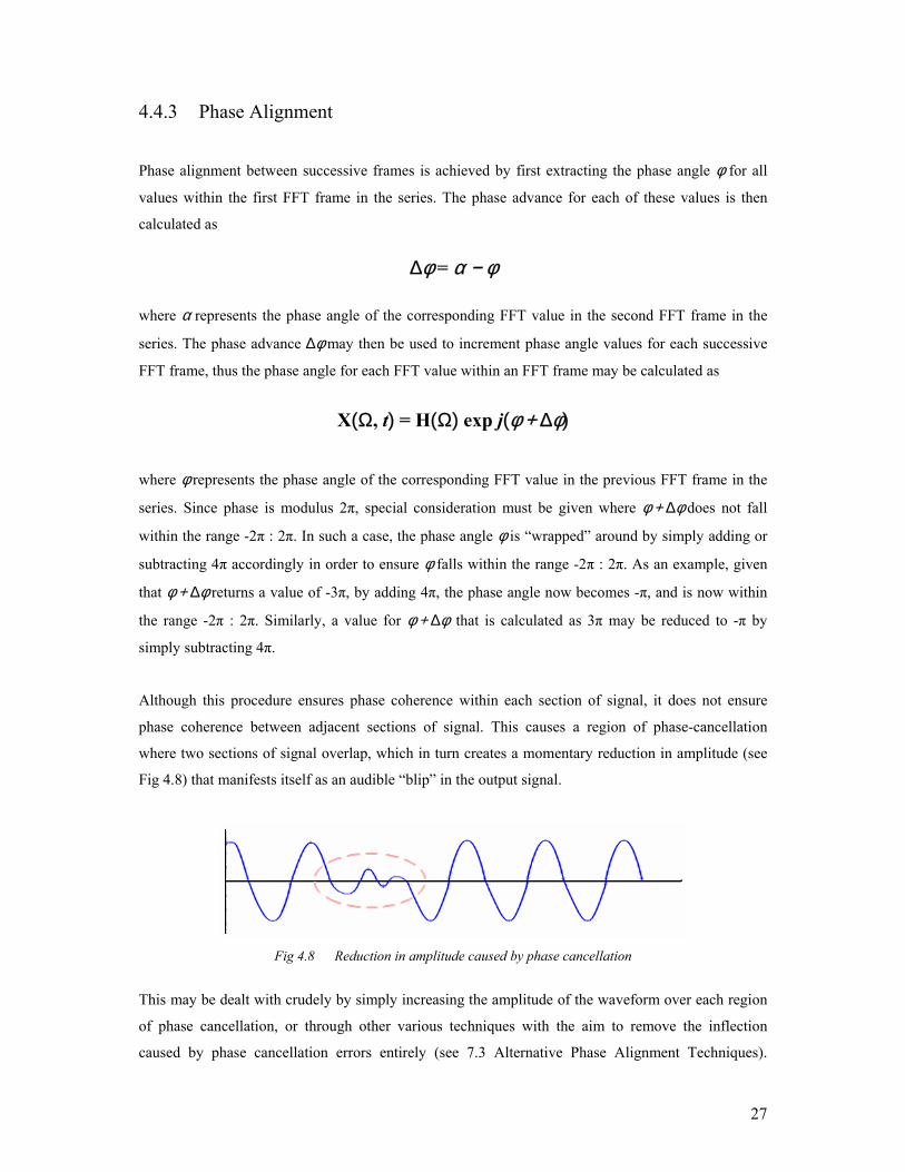
Although this procedure ensures phase coherence within each section of signal, it does not ensure

phase coherence between adjacent sections of signal. This causes a region of phase-cancellation

where two sections of signal overlap, which in turn creates a momentary reduction in amplitude (see

Fig 4.8) that manifests itself as an audible “blip” in the output signal.

Fig 4.8 Reduction in amplitude caused by phase cancellation

This may be dealt with crudely by simply increasing the amplitude of the waveform over each region

of phase cancellation, or through other various techniques with the aim to remove the inflection

caused by phase cancellation errors entirely (see 7.3 Alternative Phase Alignment Techniques).

28

However, the effect may be reduced significantly through an appropriate choice of window size. As

discussed earlier (see 4.1 Converting to Frequency Domain), the use of a Hanning window provides a

“cross-fade” effect that, with a large enough window size, reduces the effects of phase cancellation

considerably and therefore removes the need for any extra signal processing.

4.5 Signal Reconstruction

Once time scaling within the frequency domain is complete, the next step is to convert each section of

the signal back to a waveform using the Inverse Fourier Transform [8]. The Inverse Fourier

Transform is identical to the Fourier Transform (see 4.1 Converting To Frequency Domain), differing

only in the sign of the exponent. Following this stage, the Fourier representation of the signal is

converted back into the time domain and thus is no longer represented as an array of complex

numbers, but as an array of real values.

As discussed earlier, the original time base of each section is restored through interpolation of the data

values representing the signal’s waveform. This creates the effect of “resampling” each section, whilst

retaining the same sampling rate, thus allowing individual sections to be resampled by different

amounts. It is important that resampling is performed in this way since conventional resampling

would affect the entire waveform and therefore non-linear pitch shifts would not be possible. The

interpolation is performed by first identifying the correct length T for each section of the input signal.

This is calculated using the following equation

T = ( ftsize + ( (N –1) * hop ) )

where N represents the number of FFT frames used in each section, hop is the window hop size

between successive FFT frames, and ftsize is the size of each FFT frame. The value T corresponds to

the number of data values that should be used to represent each section of the signal. Interpolation is

then carried out, either reducing or increasing the size of the array so that the number of data values is

equal to T, thus ensuring that any modified sections are restored to their original timebase and that all

sections within in the output signal are of equal length.

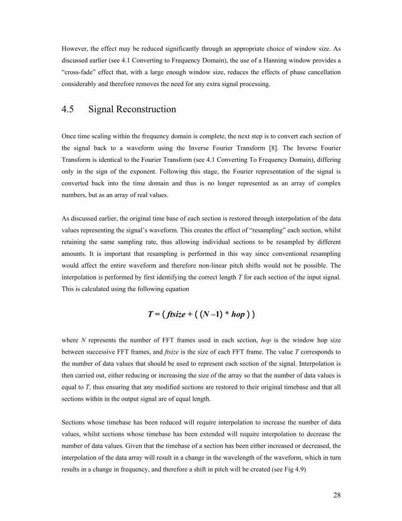
Sections whose timebase has been reduced will require interpolation to increase the number of data

values, whilst sections whose timebase has been extended will require interpolation to decrease the

number of data values. Given that the timebase of a section has been either increased or decreased, the

interpolation of the data array will result in a change in the wavelength of the waveform, which in turn

results in a change in frequency, and therefore a shift in pitch will be created (see Fig 4.9)

29

Fig 4.9 A) A simple waveform

B) Timebase of waveform is increased by a factor of two

C) “Resampled” waveform – frequency is now increased by a factor of two

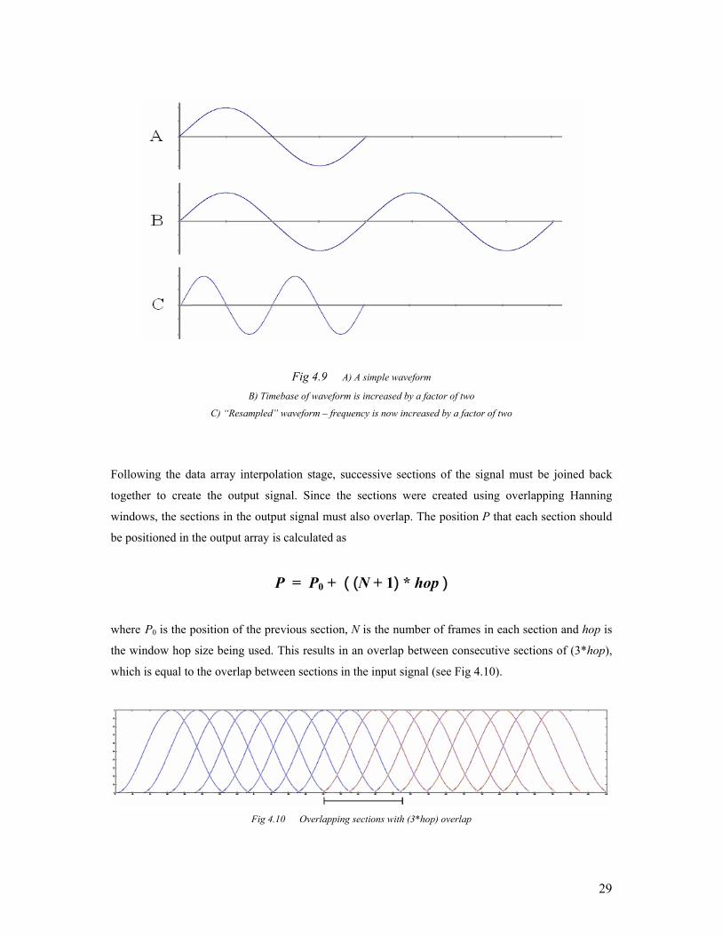
Following the data array interpolation stage, successive sections of the signal must be joined back

together to create the output signal. Since the sections were created using overlapping Hanning

windows, the sections in the output signal must also overlap. The position P that each section should

be positioned in the output array is calculated as

P = P0 + ( (N + 1) * hop )

where P0 is the position of the previous section, N is the number of frames in each section and hop is

the window hop size being used. This results in an overlap between consecutive sections of (3*hop),

which is equal to the overlap between sections in the input signal (see Fig 4.10).

Fig 4.10 Overlapping sections with (3*hop) overlap

30

5 Evaluation

5.1 Evaluation Criteria 5.1.1 Analytical Evaluation Evaluation of the Automatic Pitch Correction System was divided into two separate stages. The first

stage used analytical testing within the Matlab environment to test the accuracy of the individual

modules. Testing of the Pitch Detection and Pitch correction modules involved inputting a signal of

known frequency and observing the output of each module. Throughout this procedure, different

source signals with varying amounts of harmonics and overtones were required in order to ensure

each module could cope with a wide range of input material. Graphical output within Matlab, and

frequency values obtained through testing on an external machine (see Appendix C), provided

comprehensive results that enabled error calculations to be made.

5.1.2 Qualitative Evaluation The ultimate goal of an automatic pitch-correction system is to achieve a result that is pleasing to the

human ear and therefore the method of evaluation for such a system should reflect this. For this

reason, the second stage of evaluation involved subjective human testing in order to assess the output

qualitatively, where the results depend solely on how the pitch correction sounds to the human ear.

Qualitative evaluation was implemented by assembling a group of external judges (chosen from a

selection of musicians and non-musicians). The system’s performance was then evaluated with

respect to its ability to recreate the characteristics of the original sound, focussing on the importance

of creating a desirable output that is pleasing to the human ear.

5.1.3 Tolerance Analysis Throughout evaluation of the Automatic Pitch Correction System, every effort was made to ensure

that the input test files contained as diverse a range of audio material as possible. Different

instruments produce waveforms that behave very differently and contain vastly differing numbers of

harmonics and overtones. Another important consideration is the fact that frequency vs. pitch is a

logarithmic scale (see 4.3.1 Pitch Perception and Frequency of Musical Notes); higher pitched notes

are separated by a larger degree than lower frequencies and therefore lower frequencies require

greater accuracy to produce an acceptable result. Each module was tested for accuracy with many

different instruments over a wide range of frequencies, varying from very low notes played on a bass

guitar, to very high notes played on a violin. This enabled the identification of a frequency threshold

value, below which the accuracy of the system was found to deteriorate unacceptably.

31

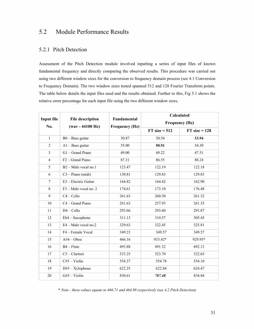
5.2 Module Performance Results

5.2.1 Pitch Detection

Assessment of the Pitch Detection module involved inputting a series of input files of known

fundamental frequency and directly comparing the observed results. This procedure was carried out

using two different window sizes for the conversion to frequency domain process (see 4.1 Conversion

to Frequency Domain). The two window sizes tested spanned 512 and 128 Fourier Transform points.

The table below details the input files used and the results obtained. Further to this, Fig 5.1 shows the

relative error percentage for each input file using the two different window sizes.

* Note - these values equate to 466.71 and 464.98 respectively (see 4.2 Pitch Detection)

Calculated

Frequency (Hz) Input file

No.

File description

(wav - 44100 Hz)

Fundamental

Frequency (Hz)FT size = 512 FT size = 128

1 B0 – Bass guitar 30.87 30.54 33.94

2 A1 – Bass guitar 55.00 50.91 54.30

3 G1 – Grand Piano 49.00 49.22 47.51

4 F2 – Grand Piano 87.31 86.55 88.24

5 B2 – Male vocal no.1 123.47 122.19 122.18

6 C3 – Piano (midi) 130.81 129.83 129.83

7 E3 – Electric Guitar 164.82 164.42 162.90

8 F3 – Male vocal no. 2 174.61 173.10 176.48

9 C4 – Cello 261.63 260.50 261.32

10 C4 – Grand Piano 261.63 257.93 261.35

11 D4 – Cello 293.66 293.60 291.87

12 Eb4 – Saxophone 311.13 310.57 305.45

13 E4 – Male vocal no.2 329.63 322.45 325.81

14 F4 – Female Vocal 349.23 349.57 349.57

15 A#4 – Oboe 466.16 933.42* 929.95*

16 B4 – Flute 493.88 491.32 492.12

17 C5 – Clarinet 523.25 523.70 522.65

18 C#5 – Violin 554.37 554.78 554.10

19 D#5 – Xylophone 622.25 622.84 624.47

20 G#5 – Violin 830.61 707.48 834.84

32

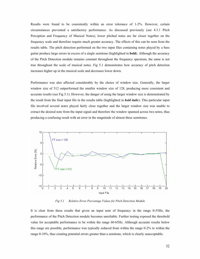
Results were found to be consistently within an error tolerance of 1-2%. However, certain

circumstances prevented a satisfactory performance. As discussed previously (see 4.3.1 Pitch

Perception and Frequency of Musical Notes), lower pitched notes are far closer together on the

frequency scale and therefore require much greater accuracy. The effects of this can be seen from the

results table. The pitch detection performed on the two input files containing notes played by a bass

guitar produce large errors in excess of a single semitone (highlighted in bold). Although the accuracy

of the Pitch Detection module remains constant throughout the frequency spectrum, the same is not

true throughout the scale of musical notes. Fig 5.1 demonstrates how accuracy of pitch detection

increases higher up in the musical scale and decreases lower down.

Performance was also affected considerably by the choice of window size. Generally, the larger

window size of 512 outperformed the smaller window size of 128, producing more consistent and

accurate results (see Fig 5.1). However, the danger of using the larger window size is demonstrated by

the result from the final input file in the results table (highlighted in bold italic). This particular input

file involved several notes played fairly close together and the larger window size was unable to

extract the desired note from the input signal and therefore the window spanned across two notes, thus

producing a confusing result with an error in the magnitude of almost three semitones.

Fig 5.1 Relative Error Percentage Values for Pitch Detection Module

It is clear from these results that given an input note of frequency in the range 0-55Hz, the

performance of the Pitch Detection module becomes unreliable. Further testing exposed the threshold

value for acceptable performance to be within the range 60-65Hz. Although accurate results below

this range are possible, performance was typically reduced from within the range 0-2% to within the

range 0-10%, thus creating potential errors greater than a semitone, which is clearly unacceptable.

33

5.2.2 Pitch Correction

Assessment of the performance of the Pitch Correction module involved two stages. Firstly, input

files containing notes of known frequency were subject to a pitch-shifting process on an external

machine (see Appendix C) to an arbitrary frequency not more than one semitone away. The new

fundamental frequency was then calculated. For accuracy reasons, this was performed using an

external machine (see Appendix C). The Pitch Correction module was then tested using these files

and knowledge of both the fundamental and target frequencies for each note. The second stage

involved the verification of the newly shifted pitch. Again, for accuracy reasons, this was performed

on an external machine (see Appendix C).

Tests were run using two different values for N (see 4.4 Pitch Correction), where N represents the

number of FFT frames present for each pitch-shifted section of signal. The first series of tests used N

= 100, whilst the second used N = 200. These values for N allow for 1% and 0.5% pitch shifts

respectively (see 4.4 Pitch Correction). The table below displays the results obtained.

Pitch-shifted Frequency

(Hz) Input file

No.

File description

(wav - 44100 Hz)

Fundamental

Frequency

(Hz)

Target

Frequency

(Hz) 100 Frames 200 Frames

1 B0 – Bass guitar 30 30.87 (B0) 31 31 2 A1 – Bass guitar 54 55.00 (A1) 55 55 3 G1 – Grand Piano 50 49.00 (G1) 49 49 4 F2 – Grand Piano 85 87.31 (F2) 88 87 5 B2 – Male vocal no.1 120 123.47 (B2) 124 123 6 C3 – Piano (midi) 134 130.81 (C3) 132 131 7 E3 – Electric Guitar 170 164.82 (E3) 165 165 8 F3 – Male vocal no. 2 172 174.61 (F3) 174 174 9 C4 – Cello 255 261.63 (C4) 261 261

10 C4 – Grand Piano 265 261.63 (C4) 262 262 11 D4 – Cello 300 293.66 (D4) 293 294 12 Eb4 – Saxophone 305 311.13 (Eb4) 311 311 13 E4 – Male vocal no.2 335 329.63 (E4) 328 329 14 F4 – Female Vocal 340 349.23 (F4) 347 349 15 A#4 – Oboe 475 466.16 (A#4) 465 465 16 B4 – Flute 505 493.88 (B4) 495 495 17 C5 – Clarinet 510 523.25 (C5) 520 523 18 C#5 – Violin 570 554.37 (C#5) 553 556 19 D#5 – Xylophone 610 622.25 (D#5) 622 622 20 G#5 – Violin 850 830.61 (G#5) 833 829

34

Fig 5.2 demonstrates the performance of the Pitch Correction module with respect to the relative

errors between Target Frequencies and actual Pitch-Shifted Frequencies. Since pitch correction is

implemented to shift pitch on a relative scale (see 4.4 Pitch Correction), the relative errors remain

consistent throughout the frequency spectrum, falling in most cases below 0.8%.

Fig 5.2 Relative Error Percentage Values for Pitch Correction Module

However, as can be seen from the results table, the external machine used to verify both the

fundamental frequency and the pitch-shifted frequency provided accuracy to the order of 1Hz only.

Since both the fundamental frequency and the pitch-shifted frequency may vary by as much as 0.5Hz,

there is a potential rounding error within the results displayed in Fig 5.2. Given the worst-case

scenario, the rounding error could be as great as 1Hz. Fig 5.3 displays the corrected relative error

values for the Pitch Correction module, allowing for the maximum potential rounding error.

Fig 5.3 Relative Error Percentage Values for Pitch Correction Module, with maximum rounding error

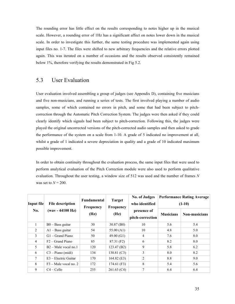
35

The rounding error has little effect on the results corresponding to notes higher up in the musical

scale. However, a rounding error of 1Hz has a significant affect on notes lower down in the musical

scale. In order to investigate this further, the same testing procedure was implemented again using

input files no. 1-7. The files were shifted to new arbitrary frequencies and the relative errors plotted

again. This was iterated on a number of occasions and the results observed consistently remained

below 1%, therefore verifying the results demonstrated in Fig 5.2.

5.3 User Evaluation User evaluation involved assembling a group of judges (see Appendix D), containing five musicians

and five non-musicians, and running a series of tests. The first involved playing a number of audio

samples, some of which contained no errors in pitch, and some that had been subject to pitch-

correction through the Automatic Pitch Correction System. The judges were then asked if they could

clearly identify which signals had been subject to pitch-correction. Following this, the judges were

played the original uncorrected versions of the pitch-corrected audio samples and then asked to grade

the performance of the system on a scale from 1-10. A grade of 5 indicated no improvement at all,

whilst a grade of 1 indicated a severe depreciation in quality and a grade of 10 indicated maximum

possible improvement.

In order to obtain continuity throughout the evaluation process, the same input files that were used to

perform analytical evaluation of the Pitch Correction module were also used to perform qualitative

evaluation. Throughout the user testing, a window size of 512 was used and the number of frames N

was set to N = 200.

Performance Rating Average

(1-10) Input file

No.

File description

(wav - 44100 Hz)

Fundamental

Frequency

(Hz)

Target

Frequency

(Hz)

No. of Judges

who identified

presence of

pitch-correctionMusicians Non-musicians

1 B0 – Bass guitar 30 30.87 (B0) 10 5.6 5.4 2 A1 – Bass guitar 54 55.00 (A1) 10 4.8 5.0 3 G1 – Grand Piano 50 49.00 (G1) 4 7.6 8.0 4 F2 – Grand Piano 85 87.31 (F2) 6 8.2 8.0 5 B2 – Male vocal no.1 120 123.47 (B2) 9 5.8 6.2 6 C3 – Piano (midi) 134 130.81 (C3) 3 8.0 8.2 7 E3 – Electric Guitar 170 164.82 (E3) 2 8.8 9.0 8 F3 – Male vocal no. 2 172 174.61 (F3) 8 5.4 5.6 9 C4 – Cello 255 261.63 (C4) 7 6.4 6.4

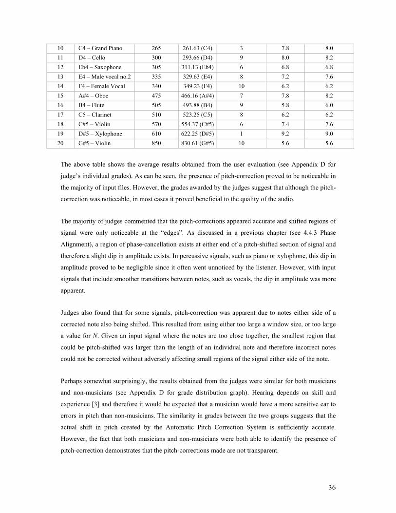
36

10 C4 – Grand Piano 265 261.63 (C4) 3 7.8 8.0 11 D4 – Cello 300 293.66 (D4) 9 8.0 8.2 12 Eb4 – Saxophone 305 311.13 (Eb4) 6 6.8 6.8 13 E4 – Male vocal no.2 335 329.63 (E4) 8 7.2 7.6 14 F4 – Female Vocal 340 349.23 (F4) 10 6.2 6.2 15 A#4 – Oboe 475 466.16 (A#4) 7 7.8 8.2 16 B4 – Flute 505 493.88 (B4) 9 5.8 6.0 17 C5 – Clarinet 510 523.25 (C5) 8 6.2 6.2 18 C#5 – Violin 570 554.37 (C#5) 6 7.4 7.6 19 D#5 – Xylophone 610 622.25 (D#5) 1 9.2 9.0 20 G#5 – Violin 850 830.61 (G#5) 10 5.6 5.6

The above table shows the average results obtained from the user evaluation (see Appendix D for

judge’s individual grades). As can be seen, the presence of pitch-correction proved to be noticeable in

the majority of input files. However, the grades awarded by the judges suggest that although the pitch-

correction was noticeable, in most cases it proved beneficial to the quality of the audio.

The majority of judges commented that the pitch-corrections appeared accurate and shifted regions of

signal were only noticeable at the “edges”. As discussed in a previous chapter (see 4.4.3 Phase

Alignment), a region of phase-cancellation exists at either end of a pitch-shifted section of signal and

therefore a slight dip in amplitude exists. In percussive signals, such as piano or xylophone, this dip in

amplitude proved to be negligible since it often went unnoticed by the listener. However, with input

signals that include smoother transitions between notes, such as vocals, the dip in amplitude was more

apparent.

Judges also found that for some signals, pitch-correction was apparent due to notes either side of a

corrected note also being shifted. This resulted from using either too large a window size, or too large

a value for N. Given an input signal where the notes are too close together, the smallest region that

could be pitch-shifted was larger than the length of an individual note and therefore incorrect notes

could not be corrected without adversely affecting small regions of the signal either side of the note.

Perhaps somewhat surprisingly, the results obtained from the judges were similar for both musicians

and non-musicians (see Appendix D for grade distribution graph). Hearing depends on skill and

experience [3] and therefore it would be expected that a musician would have a more sensitive ear to

errors in pitch than non-musicians. The similarity in grades between the two groups suggests that the

actual shift in pitch created by the Automatic Pitch Correction System is sufficiently accurate.

However, the fact that both musicians and non-musicians were both able to identify the presence of

pitch-correction demonstrates that the pitch-corrections made are not transparent.

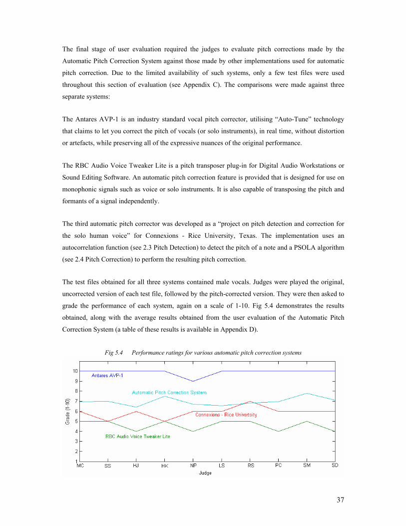
37

The final stage of user evaluation required the judges to evaluate pitch corrections made by the

Automatic Pitch Correction System against those made by other implementations used for automatic

pitch correction. Due to the limited availability of such systems, only a few test files were used

throughout this section of evaluation (see Appendix C). The comparisons were made against three

separate systems:

The Antares AVP-1 is an industry standard vocal pitch corrector, utilising “Auto-Tune” technology

that claims to let you correct the pitch of vocals (or solo instruments), in real time, without distortion

or artefacts, while preserving all of the expressive nuances of the original performance.

The RBC Audio Voice Tweaker Lite is a pitch transposer plug-in for Digital Audio Workstations or

Sound Editing Software. An automatic pitch correction feature is provided that is designed for use on

monophonic signals such as voice or solo instruments. It is also capable of transposing the pitch and

formants of a signal independently.

The third automatic pitch corrector was developed as a “project on pitch detection and correction for

the solo human voice” for Connexions - Rice University, Texas. The implementation uses an

autocorrelation function (see 2.3 Pitch Detection) to detect the pitch of a note and a PSOLA algorithm

(see 2.4 Pitch Correction) to perform the resulting pitch correction.

The test files obtained for all three systems contained male vocals. Judges were played the original,

uncorrected version of each test file, followed by the pitch-corrected version. They were then asked to

grade the performance of each system, again on a scale of 1-10. Fig 5.4 demonstrates the results

obtained, along with the average results obtained from the user evaluation of the Automatic Pitch

Correction System (a table of these results is available in Appendix D).

Fig 5.4 Performance ratings for various automatic pitch correction systems

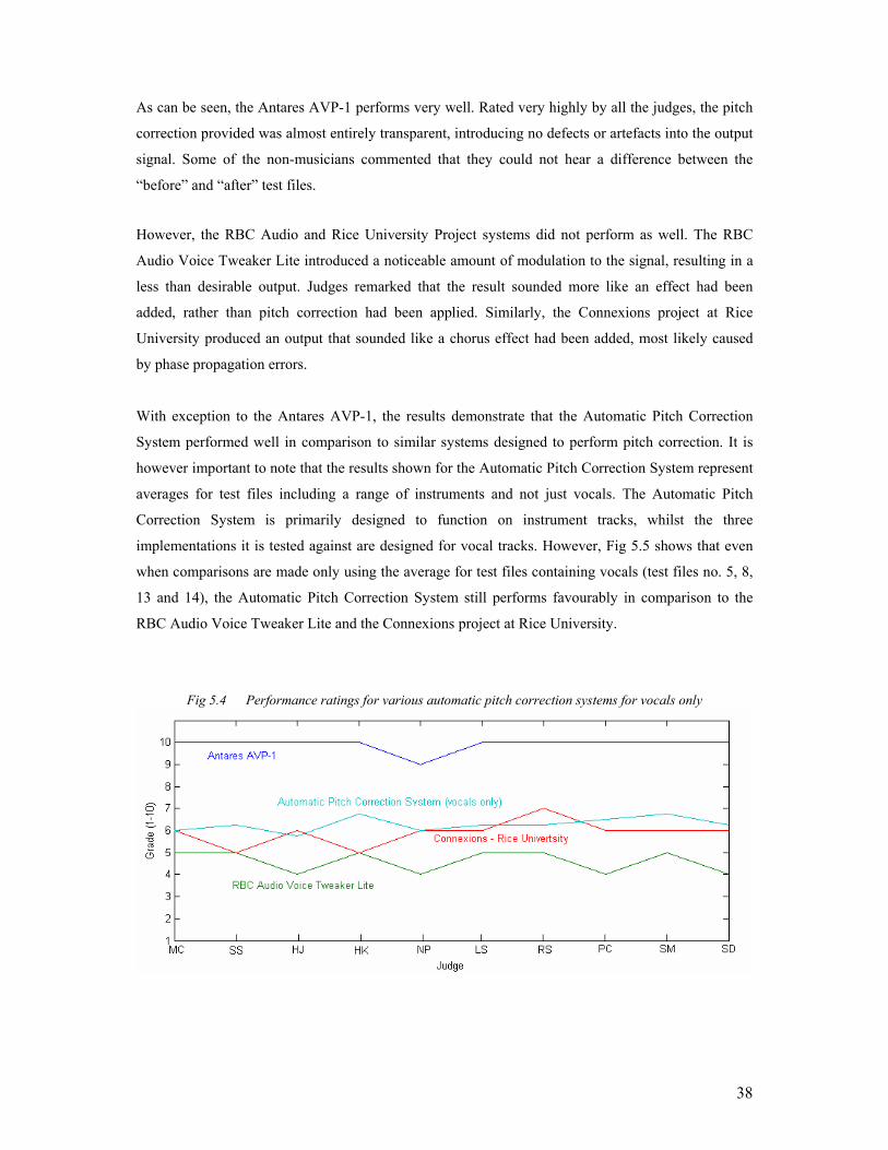
38

As can be seen, the Antares AVP-1 performs very well. Rated very highly by all the judges, the pitch

correction provided was almost entirely transparent, introducing no defects or artefacts into the output

signal. Some of the non-musicians commented that they could not hear a difference between the

“before” and “after” test files.

However, the RBC Audio and Rice University Project systems did not perform as well. The RBC

Audio Voice Tweaker Lite introduced a noticeable amount of modulation to the signal, resulting in a

less than desirable output. Judges remarked that the result sounded more like an effect had been

added, rather than pitch correction had been applied. Similarly, the Connexions project at Rice

University produced an output that sounded like a chorus effect had been added, most likely caused

by phase propagation errors.

With exception to the Antares AVP-1, the results demonstrate that the Automatic Pitch Correction

System performed well in comparison to similar systems designed to perform pitch correction. It is

however important to note that the results shown for the Automatic Pitch Correction System represent

averages for test files including a range of instruments and not just vocals. The Automatic Pitch

Correction System is primarily designed to function on instrument tracks, whilst the three

implementations it is tested against are designed for vocal tracks. However, Fig 5.5 shows that even

when comparisons are made only using the average for test files containing vocals (test files no. 5, 8,

13 and 14), the Automatic Pitch Correction System still performs favourably in comparison to the

RBC Audio Voice Tweaker Lite and the Connexions project at Rice University.

Fig 5.4 Performance ratings for various automatic pitch correction systems for vocals only

39

6 Conclusions

6.1 Evaluation of Minimum Requirements

• Discuss current methods and implementations used for detecting and correcting pitch errors

both in real time and in batch processing

Many different techniques were researched and studied. These included both frequency and time

domain techniques, the advantages and disadvantages of each method were identified and the possible

application of each method within the Automatic Pitch Correction System was considered. A range of

extra material including areas such as human pitch perception and formant correction was also

covered in order to gain a deeper understanding of the subject area.

• Create a system that is capable of detecting and correcting pitch errors on a single, simple

instrument track, or tuning fork, without introducing distortion, phase errors, or other

artefacts

The system created is able to automatically detect errors in pitch, determine an appropriate “target

note”, and shift the pitch of the appropriate section of signal to the desired frequency. Analytical

evaluation revealed that the system is able to detect pitch within an error margin of 1-2% and perform

pitch correction to accuracy within 0.8% of the target note. The maximum accumulative error that may

occur from the combined process of pitch detection and pitch correction is therefore 2.8%. The human

ear can detect differences of as little as 1 Hz in sustained notes [12], and therefore, given an input note

above “Middle C” (C4), the resulting pitch shift is known to be accurate within human hearing

capabilities. However, this is given the worst-case scenario; qualitative evaluation demonstrated that

even below Middle C, the pitch correction proved to be sufficiently accurate for a group of both

musicians and non-musicians.

Further qualitative evaluation showed that the system was able to perform automatic pitch correction

on simple instrument tracks without introducing audible loss or coloration of signal quality. The pitch

corrections performed on instrument tracks that included piano, xylophone and electric guitar were in

most cases undetectable by the majority of judges. The system was found to perform well on more

percussive tracks where note accents are quite apparent and note changes are not too closely spaced.

This is due to the choice of window size and value for N (no. of frames per pitch shifted section); a

larger window size and value for N increases the accuracy of the system, but a trade-off is made

between time and frequency resolution. A small window size and a smaller value for N prevents the

40

unwanted pitch shifting of notes that may occur with a larger window size and value for N (see 5.3

User Evaluation), but accuracy is lost due to a decreased number of frequency bins available for pitch

detection (see 4.2 Pitch Detection) and a decreased accuracy with which pitch-shifting can be

performed (see 4.4 Pitch Correction).

• Evaluate system against current implementations already used for automatic pitch correction

During user evaluation, the performance of the system was directly compared to three existing

implementations (see 5.3 User Evaluation). These implementations included a professional industry

standard vocal pitch corrector, another university research project and a pitch transposer plug-in for

computer recording software. Further evaluation was carried out to assess the system from both an

analytical and a qualitative point of view, obtaining results that demonstrated both the error tolerance

of the system and the subjective opinions of a group of judges.

6.2 Evaluation of Possible Extensions

• Perform automatic pitch-correction of input track in real-time, allowing for application in

live performances and real-time monitoring

Although this particular extension to the minimum requirements was not realised, the design and

implementation of the Automatic Pitch Correction System throughout the project was focussed on

producing a solution that could potentially be created as a real-time application. The system has

therefore been designed to run sequentially and requires no post-processing or feedback loops.

Although to obtain best results, a small delay would be required (to allow for a larger window size

and therefore increased accuracy); the system does form the basis from which a real-time application

may be implemented.

• Implement a feature that will allow a specific key to be selected before signal input. This

would enable out of pitch notes to be shifted to the nearest note in the selected key, as

opposed to the nearest note in the chromatic scale

Error detection is performed using a lookup table to determine the target note for each given

frequency. The musical scale from which target notes are chosen is purely dictated by the content of

the lookup table. By only including the frequencies for notes within a given musical scale (i.e. C

major), all notes can be shifted only to those frequencies and hence only that musical scale. Similarly,

only frequencies corresponding to notes within a given melody may be included in the lookup table

and therefore pitch-shifting may be made to a specific tune or melody.

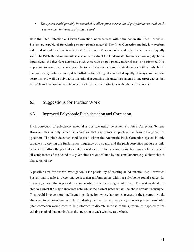
41

• The system could possibly be extended to allow pitch-correction of polyphonic material, such

as a de-tuned instrument playing a chord

Both the Pitch Detection and Pitch Correction modules used within the Automatic Pitch Correction

System are capable of functioning on polyphonic material. The Pitch Correction module is waveform

independent and therefore is able to shift the pitch of monophonic and polyphonic material equally

well. The Pitch Detection module is also able to extract the fundamental frequency from a polyphonic

input signal and therefore automatic pitch correction on polyphonic material may be performed. It is

important to note that is not possible to perform corrections on single notes within polyphonic

material; every note within a pitch-shifted section of signal is affected equally. The system therefore

performs very well on polyphonic material that contains mistuned instruments or incorrect chords, but

is unable to function on material where an incorrect note coincides with other correct notes.

6.3 Suggestions for Further Work 6.3.1 Improved Polyphonic Pitch detection and Correction

Pitch correction of polyphonic material is possible using the Automatic Pitch Correction System.

However, this is only under the condition that any errors in pitch are uniform throughout the

spectrum. The pitch detection module used within the Automatic Pitch Correction system is only

capable of detecting the fundamental frequency of a sound, and the pitch correction module is only

capable of shifting the pitch of an entire sound and therefore accurate corrections may only be made if

all components of the sound at a given time are out of tune by the same amount e.g. a chord that is

played out of key.

A possible area for further investigation is the possibility of creating an Automatic Pitch Correction

System that is able to detect and correct non-uniform errors within a polyphonic sound source, for

example, a chord that is played on a guitar where only one string is out of tune. The system should be

able to correct the single incorrect note whilst the correct notes within the chord remain unchanged.

This would involve more intelligent pitch detection, where harmonics present in the spectrum would

also need to be considered in order to identify the number and frequency of notes present. Similarly,

pitch correction would need to be performed to discrete sections of the spectrum as opposed to the

existing method that manipulates the spectrum at each window as a whole.

42

6.3.2 Real-time Automatic Pitch Correction Although the Automatic Pitch Correction System has been designed as a sequential process and

computational expense has been considered at every stage, the system still functions primarily as a

post-processor. The implementation of the Automatic Pitch Correction as a real-time application

would require actual implementation of the solution as a sequential process as well as evaluating the

possibility of optimisation and adjustments that could be made to the existing algorithms used.

The current implementation of the Automatic Pitch Correction system is still based entirely MATLAB

and therefore any further work involving real-time processing will require implementation within a

language such as C or Java, which unlike Matlab, will allow for real-time input streaming of data.

6.3.3 Pitch Correction with Formant Preservation Further work could be carried out, implementing a similar solution to automatic pitch correction that

also considers the position of formants. The existing technique used for pitch correction shifts formant

information as well as pitch. However, formants are consistent in structure and independent of pitch

[23] and therefore some form of formant preservation should be incorporated into the system.

The Automatic Pitch Correction System shifts pitch by at most half a semitone, correcting to a

chromatic scale (or one semitone, correcting to a given musical scale), and therefore for these small

shifts in pitch, the effect of shifting formants may not be apparent. However, for a more flexible

implementation that may be used to shift pitch by larger amounts, for example, the transposition of a

vocal track by more than one key, formant correction or preservation would be required.

6.3.4 Intelligent Error Correction The current implementation simply uses a “nearest neighbour” approach to error correction, whereby

a frame is shifted to either the nearest semitone (given chromatic tuning) or the nearest note in a given

musical scale. However, this may not always lead to the correct choice of target note, since an

instrument may be out of tune or a singer may sing off key by more than half a semitone. An

intelligent system could be developed that would calculate a target note that is based on the

frequencies of previous frames as well as the frequency of the current frame. One option would be to

incorporate the use of a Markov Model that would be able to predict standard note progressions and

musical scales. This would remove the need to hard code the desired musical scale to correct to (given

the chromatic scale is not to be used) and would cope with the problem of “accidentals” being

undesirably corrected.

43

7 Alternative Methods

This section covers various alternative methods that were implemented as an attempt to solve the

problem of real-time automatic pitch correction. Each method was implemented and tested, but

rejected due to the limitations or ineffectiveness of the solution.

7.1 Note Detection

A method that was initially proposed in order to perform pitch detection involved the detection of

individual notes within the input signal. Through the detection of peaks in amplitude over a given

time, the transient (or “attack”) of each note can be identified and the length of each note can be

calculated. The peaks are identified by first calculating the power spectrum for windowed sections of

the input signal. The maximum peak within each power spectrum is identified as the amplitude value

for the signal at the given time point. A plot of consecutive amplitude values is then created, thus

allowing for transients to be detected through detection of peaks within the amplitude plot.

The benefit of such an approach is that the windowing can be dynamically altered. The detection and

correction of a note need only be performed between the boundaries of the note, improving the

performance of both the pitch detection and pitch correction modules.

The pitch detection algorithm (see 4.2 Pitch Detection) is optimised for each note since the pitch

detection is performed between the boundaries of each note and therefore a maximum window size is

being used. Also, windows that overlap consecutive notes within an input signal are eliminated, thus

avoiding confusing results. The “timing” of the pitch correction (see 4.4 Pitch Correction) is also

improved since the pitch shifting is guaranteed to start with the onset of each note and end before the

onset of the next. Pitch shifting that overlaps note boundaries is prevented and therefore unwanted

pitch shifts are avoided.

An important issue that would need to be addressed is the different waveforms exhibited by various

instruments. Certain instruments such as the piano or xylophone create waveforms with very distinct

peaks in amplitude that accurately represent note transients (see Fig 7.1). However, many other

instruments such as the cello or the flute produce waveforms with amplitudes that oscillate and thus a

single note may be detected as several and note boundaries may be missed since no clear peak can be

detected (see Fig 7.2).

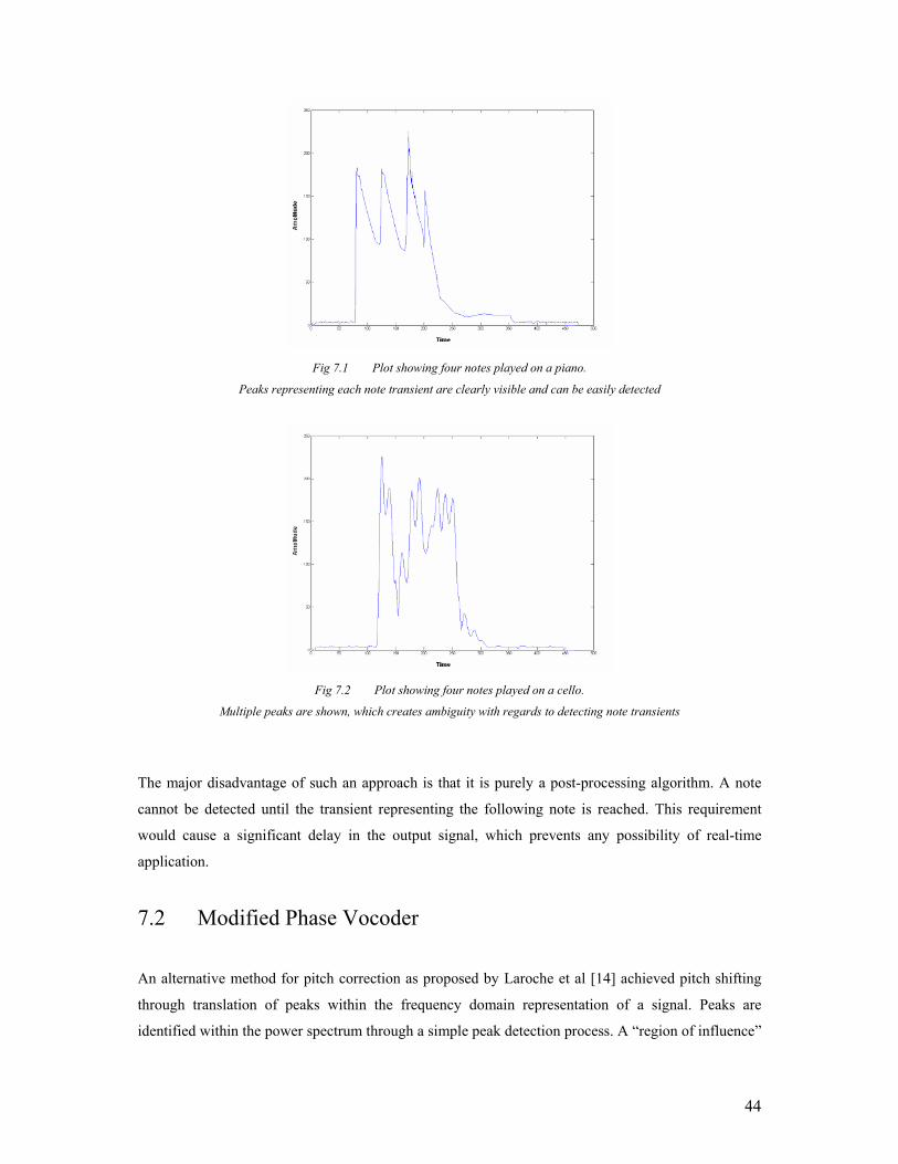
44

Fig 7.1 Plot showing four notes played on a piano.

Peaks representing each note transient are clearly visible and can be easily detected

Fig 7.2 Plot showing four notes played on a cello.

Multiple peaks are shown, which creates ambiguity with regards to detecting note transients

The major disadvantage of such an approach is that it is purely a post-processing algorithm. A note

cannot be detected until the transient representing the following note is reached. This requirement

would cause a significant delay in the output signal, which prevents any possibility of real-time

application.

7.2 Modified Phase Vocoder

An alternative method for pitch correction as proposed by Laroche et al [14] achieved pitch shifting

through translation of peaks within the frequency domain representation of a signal. Peaks are

identified within the power spectrum through a simple peak detection process. A “region of influence”

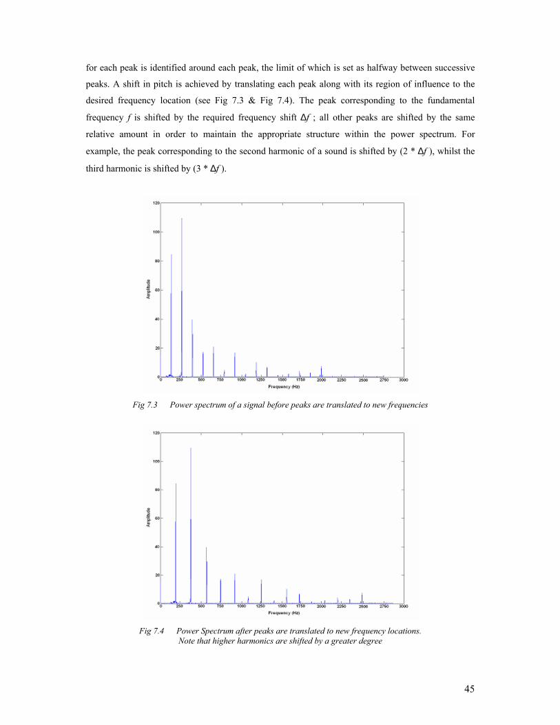
45

for each peak is identified around each peak, the limit of which is set as halfway between successive

peaks. A shift in pitch is achieved by translating each peak along with its region of influence to the

desired frequency location (see Fig 7.3 & Fig 7.4). The peak corresponding to the fundamental

frequency f is shifted by the required frequency shift ∆f ; all other peaks are shifted by the same

relative amount in order to maintain the appropriate structure within the power spectrum. For

example, the peak corresponding to the second harmonic of a sound is shifted by (2 * ∆f ), whilst the

third harmonic is shifted by (3 * ∆f ).

Fig 7.3 Power spectrum of a signal before peaks are translated to new frequencies

Fig 7.4 Power Spectrum after peaks are translated to new frequency locations.

Note that higher harmonics are shifted by a greater degree

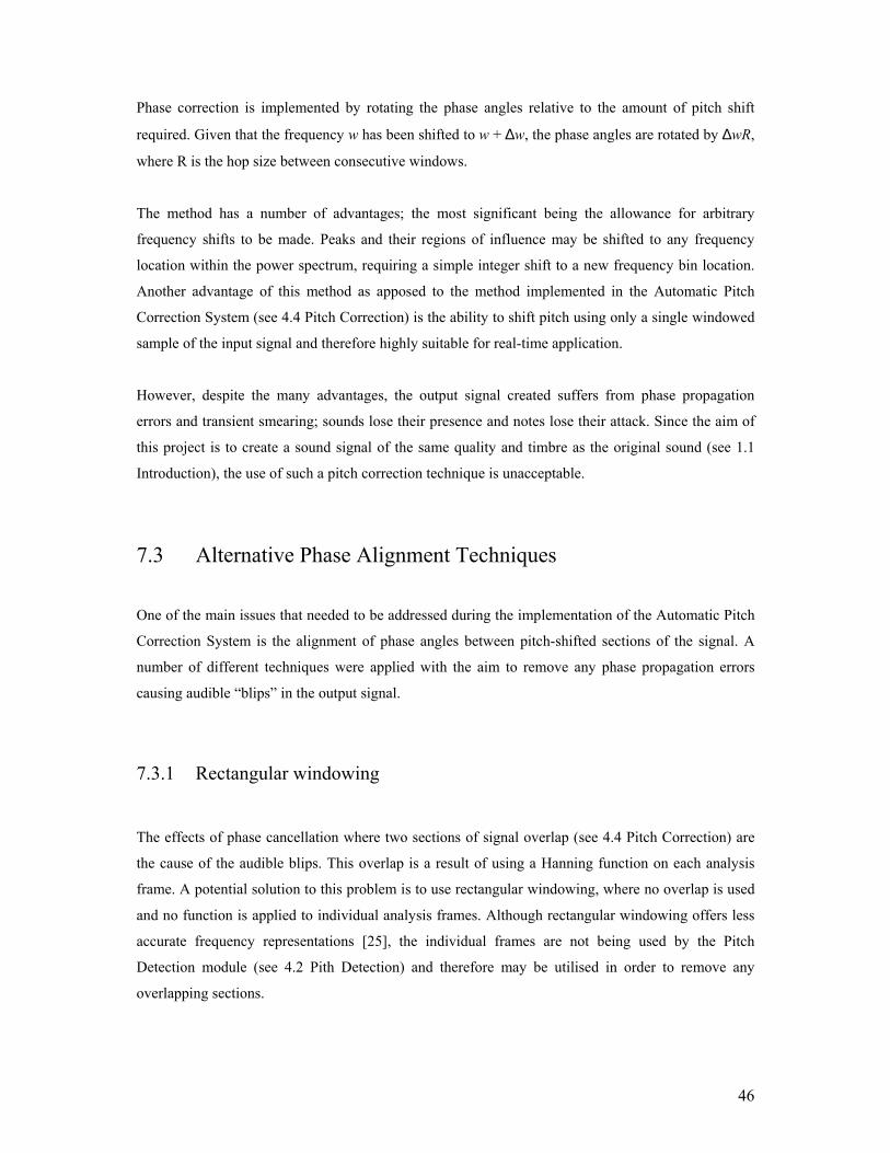
46

Phase correction is implemented by rotating the phase angles relative to the amount of pitch shift

required. Given that the frequency w has been shifted to w + ∆w, the phase angles are rotated by ∆wR,

where R is the hop size between consecutive windows.

The method has a number of advantages; the most significant being the allowance for arbitrary

frequency shifts to be made. Peaks and their regions of influence may be shifted to any frequency

location within the power spectrum, requiring a simple integer shift to a new frequency bin location.

Another advantage of this method as apposed to the method implemented in the Automatic Pitch

Correction System (see 4.4 Pitch Correction) is the ability to shift pitch using only a single windowed

sample of the input signal and therefore highly suitable for real-time application.

However, despite the many advantages, the output signal created suffers from phase propagation

errors and transient smearing; sounds lose their presence and notes lose their attack. Since the aim of

this project is to create a sound signal of the same quality and timbre as the original sound (see 1.1

Introduction), the use of such a pitch correction technique is unacceptable.

7.3 Alternative Phase Alignment Techniques

One of the main issues that needed to be addressed during the implementation of the Automatic Pitch

Correction System is the alignment of phase angles between pitch-shifted sections of the signal. A

number of different techniques were applied with the aim to remove any phase propagation errors

causing audible “blips” in the output signal.

7.3.1 Rectangular windowing

The effects of phase cancellation where two sections of signal overlap (see 4.4 Pitch Correction) are

the cause of the audible blips. This overlap is a result of using a Hanning function on each analysis

frame. A potential solution to this problem is to use rectangular windowing, where no overlap is used

and no function is applied to individual analysis frames. Although rectangular windowing offers less

accurate frequency representations [25], the individual frames are not being used by the Pitch

Detection module (see 4.2 Pith Detection) and therefore may be utilised in order to remove any

overlapping sections.

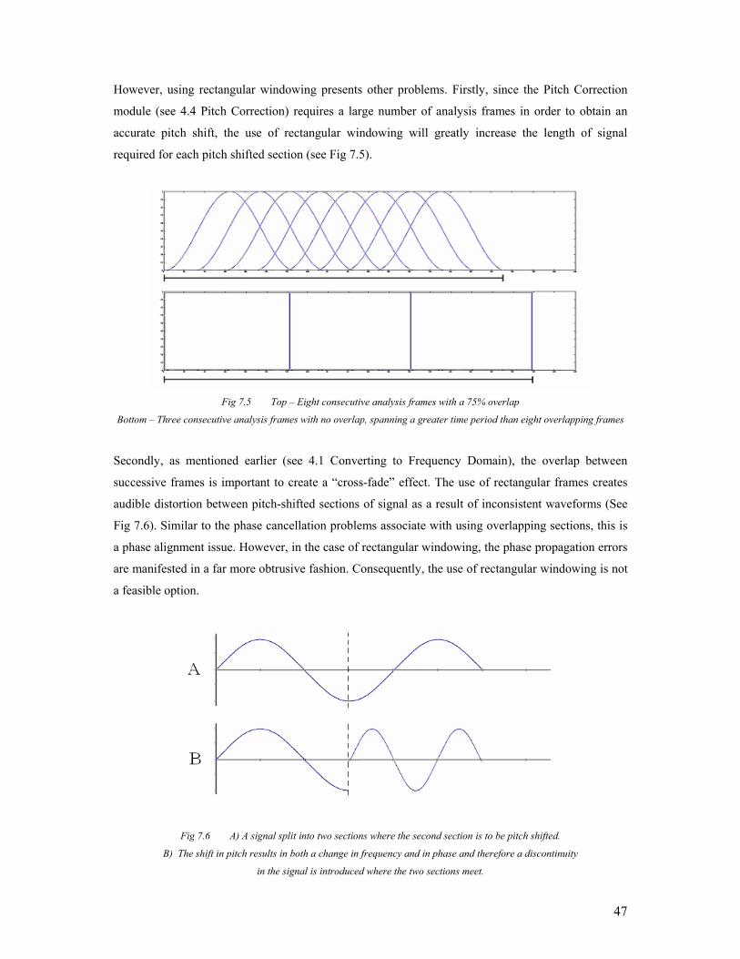
47

However, using rectangular windowing presents other problems. Firstly, since the Pitch Correction

module (see 4.4 Pitch Correction) requires a large number of analysis frames in order to obtain an

accurate pitch shift, the use of rectangular windowing will greatly increase the length of signal

required for each pitch shifted section (see Fig 7.5).

Fig 7.5 Top – Eight consecutive analysis frames with a 75% overlap

Bottom – Three consecutive analysis frames with no overlap, spanning a greater time period than eight overlapping frames

Secondly, as mentioned earlier (see 4.1 Converting to Frequency Domain), the overlap between

successive frames is important to create a “cross-fade” effect. The use of rectangular frames creates

audible distortion between pitch-shifted sections of signal as a result of inconsistent waveforms (See

Fig 7.6). Similar to the phase cancellation problems associate with using overlapping sections, this is

a phase alignment issue. However, in the case of rectangular windowing, the phase propagation errors

are manifested in a far more obtrusive fashion. Consequently, the use of rectangular windowing is not

a feasible option.

Fig 7.6 A) A signal split into two sections where the second section is to be pitch shifted.

B) The shift in pitch results in both a change in frequency and in phase and therefore a discontinuity

in the signal is introduced where the two sections meet.

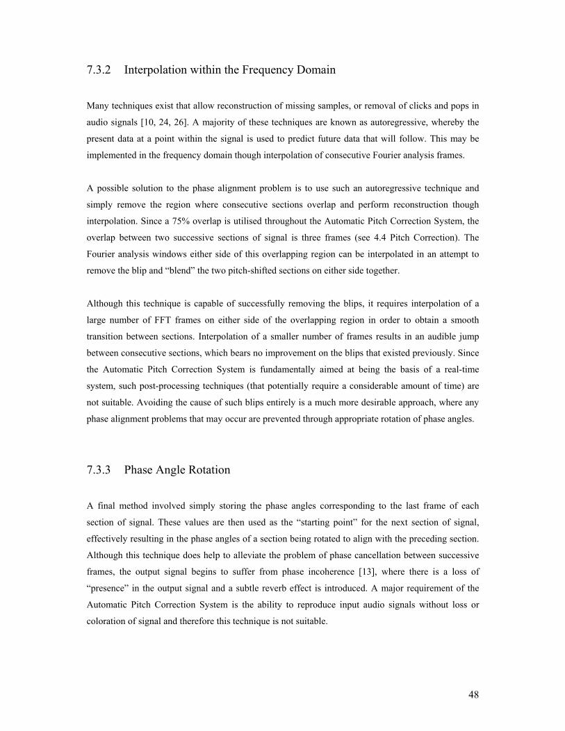
48

7.3.2 Interpolation within the Frequency Domain

Many techniques exist that allow reconstruction of missing samples, or removal of clicks and pops in

audio signals [10, 24, 26]. A majority of these techniques are known as autoregressive, whereby the

present data at a point within the signal is used to predict future data that will follow. This may be

implemented in the frequency domain though interpolation of consecutive Fourier analysis frames.

A possible solution to the phase alignment problem is to use such an autoregressive technique and

simply remove the region where consecutive sections overlap and perform reconstruction though

interpolation. Since a 75% overlap is utilised throughout the Automatic Pitch Correction System, the

overlap between two successive sections of signal is three frames (see 4.4 Pitch Correction). The

Fourier analysis windows either side of this overlapping region can be interpolated in an attempt to

remove the blip and “blend” the two pitch-shifted sections on either side together.

Although this technique is capable of successfully removing the blips, it requires interpolation of a

large number of FFT frames on either side of the overlapping region in order to obtain a smooth

transition between sections. Interpolation of a smaller number of frames results in an audible jump

between consecutive sections, which bears no improvement on the blips that existed previously. Since

the Automatic Pitch Correction System is fundamentally aimed at being the basis of a real-time

system, such post-processing techniques (that potentially require a considerable amount of time) are

not suitable. Avoiding the cause of such blips entirely is a much more desirable approach, where any

phase alignment problems that may occur are prevented through appropriate rotation of phase angles.

7.3.3 Phase Angle Rotation

A final method involved simply storing the phase angles corresponding to the last frame of each

section of signal. These values are then used as the “starting point” for the next section of signal,

effectively resulting in the phase angles of a section being rotated to align with the preceding section.

Although this technique does help to alleviate the problem of phase cancellation between successive

frames, the output signal begins to suffer from phase incoherence [13], where there is a loss of

“presence” in the output signal and a subtle reverb effect is introduced. A major requirement of the

Automatic Pitch Correction System is the ability to reproduce input audio signals without loss or

coloration of signal and therefore this technique is not suitable.

49

References

[1] A. M. Noll. 1969. “Pitch determination of human speech by the harmonic product spectrum,

the harmonic sum spectrum, and a maximum likelihood estimate”. Proc of the Symposium on

Computer Processing in Communication, pages 779–798, April 1969.

[2] Aniruddh D. Patel, Evan Balaban1. 2001. “Human pitch perception is reflected in the timing of

stimulus-related cortical activity”. The Neurosciences Institute. California, USA.

[3] B Espinoza-Varas, C. S. Watson. 1989. “Perception of complex auditory patterns by humans”.

In R.J. Dooling and S.H. Hulse (Eds.) The Comparative Psychology of Audition: Perceiving

Complex Sounds, Lawrence Erlbaum Associates, Hillsdale, NJ.

[4] Ben Gold, Nelson Morgan. 2000. “Speech and Audio Signal Processing: Processing and

Perception of Speech and Music”. John Wiley & Sons, Inc. New York

[5] Cheol-Woo Jo, Ho-Gyun Bang, William A. Ainsworth. “Improved Glottal Closure Instant

Detector Based on Linear Prediction and Standard Pitch Concept”. Dept. of Control and

Instrumentation Engineering, Changwon University, Korea.

[6] David Claus. 2004. “Nearest Neighbour, Condensing and Editing”. Computer Vision Reading

Group. Oxford.

[7] Edward A. Lee. 1998. “Design Methodology for DSP”. Department of Electrical Engineering

and Computer Science University of California, Berkeley.

[8] Glenn Zelniker, Fred J. Taylor. 1994. “Advanced Digital Signal Processing: Theory and

Applications”. Marcel Dekker, inc. New York.

[9] Goangshiuan S. Ying, Leah H. Jamieson, Carl D. Michell. 1994. “A Probabilistic Approach to

AMDF Pitch Detection”. School of Electrical and Computer Engineering, Purdue University.

[10] I. Potamitis, N. Fakotakis. 2001. “Autoregressive Time-Frequency Interpolation in the Context

of Missing Data Theory for Impulsive Noise Compensation”. Wire Communications

Laboratory, Electrical and Computer Engineering Dept, University of Patras, 261 10 Rion,

Patras, Greece.

50

[11] Jaideva C. Goswami, Andrew K. Chan. 1999. “Fundamentals of Wavelets: Theory, Algorithms

and Applications”. John Wiley & Sons, Inc. New York.

[12] James Athey. 2003. “Eartrainer: Cross-Platform Eartraining Program for Musicians”.

Retreived February 12th, 2004, from http://zoo.cs.yale.edu/classes/cs490/02-

03b/james.athey/Final_Report.html

[13] Jean Laroche, Mark Dolson. 1999. “Improved Phase Vocoder Time-Scale Modification of

Audio”. IEEE Transactions on Speech and Audio Processing, vol. 7, no. 3, pp. 323-332.

[14] Jean Laroche, Mark Dolson. 1999. “New Phase-Vocoder Techniques for Pitch Shifting,

Harmonizing and Other Exotic Effects”. Proc. IEEE Workshop on Applications of Signal

Processing to Audio and Acoustics, New Paltz. New York. pp. 91-94.

[15] Jean Laroche. 2003. “Frequency Domain Techniques for High-Quality Voice Modification”.

Proc. of the 6th int. Conference on Digital Audio Effects, London, UK, pp. dafx72.

[16] John Garas, Piet C. W. Sommen. 1998. “Time/Pitch Scaling Using the Constant-Q Phase

Vocoder”. Eindhoven University of Technology.

[17] L. K. Saul, D. D. Lee, C. L. Isbell, and Y. LeCun. 2003. “Real time voice processing with

audiovisual feedback: toward autonomous agents with perfect pitch”. In S. Becker, S. Thrun,

and K. Obermayer (eds.), Advances in Neural Information Processing Systems 15, pages 1205-

1212.

[18] L. R. Rabiner, R. W. Schafer. 1978. “Digital Processing of Speech Signals”. Prentice Hall, Inc.

New Jersey.

[19] Lawrence J. Ziomek. 1995. “Fundamentals of Acoustic Field Theory and Space-Time Signal

Processing”. CRC Press, Inc. Boca Raton.

[20] Masahiro FURUKAWA, Yusuke HIOKA, Takuro EMA, Nozomu HAMADA. 2003.

“Introducing New Mechanism in the Learning Process of FDICA-Based Speech Separation”.

International Workshop on Acoustic Echo and Noise Control, Sept. 2003, Kyoto, Japan.

51

[21] Patricio de la Cuadra, Aaron Master, Craig Sapp. 2001. “Efficient Pitch Detection Techniques

for Interactive Music”. Center for Computer Research in Music and Acoustics, Stanford

University.

[22] Paul Boersma. 1993. “Accurate Short-Term Analysis of the Fundamental Frequency and the

Harmonics-to-Noise Ratio of a Sampled Sound”. Institute of Phonetic Sciences, University of

Amsterdam, Proceedings 17 (1993), 97-110.

[23] Paul L. Browning. 1997. “Audio Digital Signal Processing in Real Time”. Computer Science

Dept. West Virginia University.

[24] Paulo A. A. Esquef, Vesa V¨alim¨aki, Kari Roth, Ismo Kauppinen. 2003. “Interpolation of

Long Gaps in Audio Signals Using the Warped Burg’s Method”. Proc. of the 6th Int.

Conference on Digital Audio Effects (DAFx-03), London, UK, September 08-11, 2003.

[25] Pierre Wickramarachi. 2003. “Effects of Windowing on the Spectral Content of a Signal”.

Sound and Vision January 2003. Data Physics Corporation, San Jose, California.

[26] R. N. J. Veldhuis. 1990. “Restoration of Lost Samples in Digital Signal”. Prentice-Hall.

[27] Simon J. Godsill and Pete J. W. Rayner. 1998. “Digital Audio Restoration: A Statistical Model

Based Approach”. Springer. London.

[28] Stephan M. Bernsee. 1995. “Time Stretching and Pitch Shifting of Audio Signals”. Retrieved:

November 20th, 2003, from http://www.dspdimension.com/html/timepitch.html

[29] Tristan Jehan. 1997. “Pitch Detection”. CNMAT. Berkeley, California. Retrieved: November

11th, 2003, from http://www.cnmat.berkeley.edu/~tristan/Report/node4.html

52

Appendix A

Reflection on Project Experience I found the project to be both an enjoyable and challenging experience. The subject area covered a

range of different topics and involved a considerable amount of learning throughout the process of

creating both the solution and the report. Mainly incorporating methodology and time management,

the following describe the lessons I have learnt throughout the duration of this project:

Background reading and thorough research within the subject area is essential. A lot of time can be

wasted embarking on the implementation stages of a project if an in-depth understanding and

knowledge of the subject area has not already been achieved. Extra time spent in the early stages of a

project can save a lot of time during the following stages and help to produce a higher quality

solution. Finding appropriate material proved to be very challenging in the early stages of the project

since very little is written about “automatic pitch correction”. However, once a greater understanding

of the subject area had been achieved, searching for and locating appropriate literature became

increasingly easier, with many useful references discovered through the use of the Internet.

Creating a time schedule is a very worthwhile process and the importance of allocating adequate time

for each project stage should be taken into consideration. Most significantly during the

implementation stages, the actual amount of time required often exceeds the predicted time and

therefore the time required for each stage should be overestimated where possible. Throughout this

project, it was found that the appropriateness of an algorithm or technique could often not be assessed

until implementation of that particular algorithm or technique was complete. This increased the time

spent implementing the solution considerably and reduced the available amount of time for other

project stages.

It is also important to identify appropriate evaluation criteria early on during the project. Without

such, the project may lack focus or direction. If the performance of a system cannot be determined

through appropriate evaluation, the reasons for selecting an appropriate methodology and choice of

implementation become ambiguous, and therefore most likely resulting in an inadequate solution.

Finally, it is important to set realistic minimum requirements and to ensure focus is directed towards

meeting the needs of the project. Time spent thinking carefully about the minimum requirements early

on in the project can prevent a lot of wasted time and ensure focus is maintained on the correct aspects

of the project.

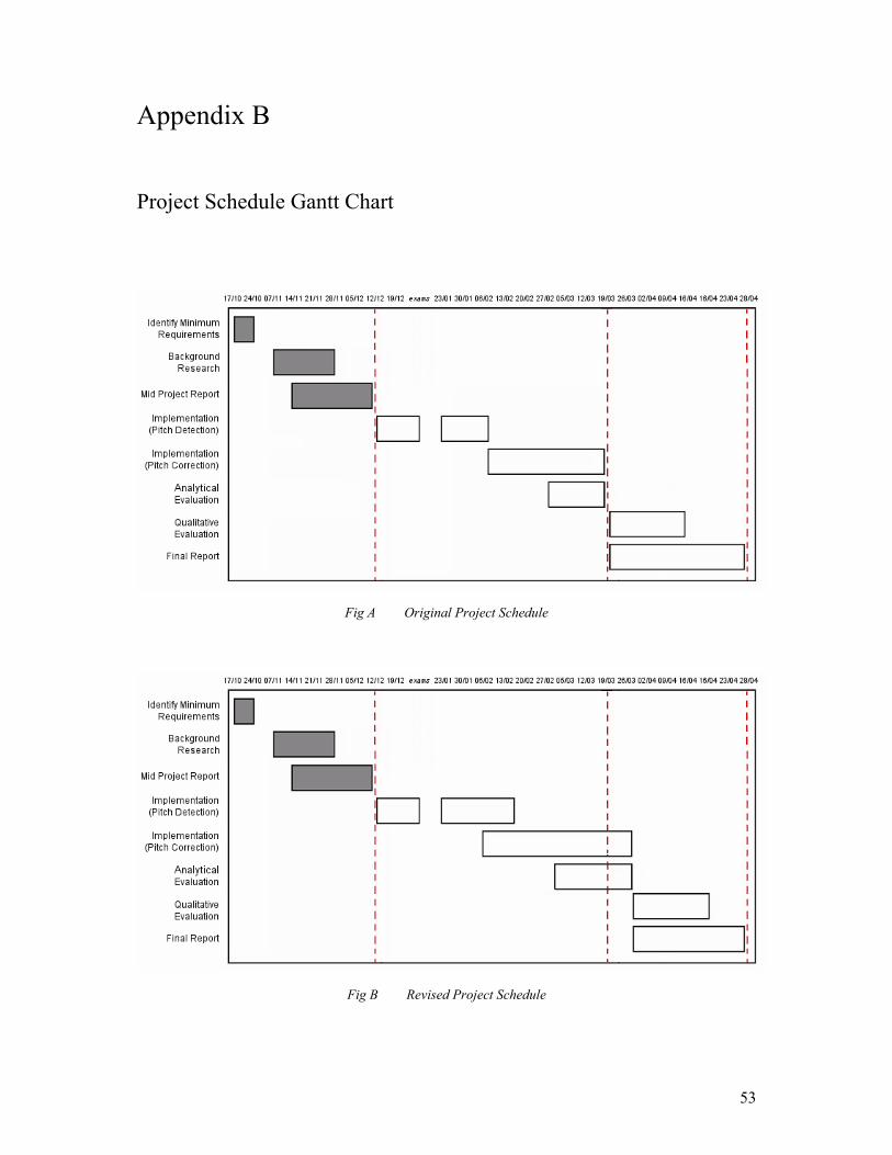
53

Appendix B Project Schedule Gantt Chart

Fig A Original Project Schedule

Fig B Revised Project Schedule

54

Appendix C

External Devices

Evaluation of the Pitch Correction module involved shifting the pitch of individual notes within

various audio samples. To implement this, an external track-editing machine was utilised, specifically,

the ZOOM MRS1608. This machine provides full editing capabilities for musical tracks and therefore

ideally suited to effect pitch errors within audio samples. The MRS1608 also provides a built-in

chromatic tuner, which was also used throughout the evaluation of the Pitch Correction module.

More information can be found at www.zoom.co.jp

Below is a list of the existing implementations used for automatic pitch correction that were used as

part of the user evaluation. Included are the URLs from which the test files were obtained:

• Antares Vocal Producer AVP-1

http://onstagemag.com/ar/performance_online_extras_january_2/

• RBC Audio Voice Tweaker Lite

http://www.rbcaudio.com/html/vt_lite.html

• “Project on pitch detection and correction for the solo human voice”

Connexions - Rice University, Texas

http://cnx.rice.edu/content/m11716/latest/

55

Appendix D

User Evaluation Results

The group of judges selected to perform user evaluation included five experienced musicians (Grade7

– Grade 8) and five non-musicians. Below is a list of the people involved, listed with their respective

instruments:

Musicians -

Michael Connolly Guitar

Simon Stevens Bass Guitar, Clarinet

Helen Jackson Piano, Flute

Helen Kirkbright Piano

Nick Parva Guitar, Drums

Non-Musicians -

Leon Savidis

Rouzbeh Safaie

Peter Coleman

Sean Matthews

Sharon Davidson

Performance Ratings -

The following table details the individual performance ratings awarded by each judges for each test

file during user evaluation. The average grade for musicians and non-musicians for each test input file

is also shown (marked as Avg). Further to this, Fig D displays the grade distribution between average

performance ratings for both the musicians and the non-musicians.

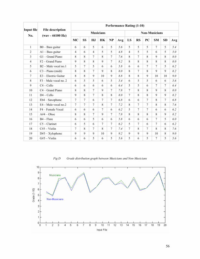
56

Performance Rating (1-10)

Musicians Non-Musicians Input file

No.

File description

(wav - 44100 Hz) MC SS HJ HK NP Avg LS RS PC SM SD Avg

1 B0 – Bass guitar 6 6 5 6 5 5.6 5 5 5 7 5 5.4 2 A1 – Bass guitar 4 6 4 5 5 4.8 4 5 5 6 5 5.0 3 G1 – Grand Piano 8 8 7 8 7 7.6 8 7 8 9 8 8.0 4 F2 – Grand Piano 9 8 8 9 7 8.2 8 8 8 8 8 8.0 5 B2 – Male vocal no.1 5 7 5 6 6 5.8 6 6 7 7 5 6.2 6 C3 – Piano (midi) 8 8 7 9 8 8.0 8 7 8 9 9 8.2 7 E3 – Electric Guitar 8 8 9 10 9 8.8 8 8 9 10 10 9.0 8 F3 – Male vocal no. 2 6 5 5 6 5 5.4 6 5 5 6 6 5.6 9 C4 – Cello 6 6 6 6 6 6.4 5 5 6 7 7 6.4

10 C4 – Grand Piano 8 8 7 9 7 7.8 7 8 8 9 8 8.0 11 D4 – Cello 9 8 7 8 8 8.0 7 8 8 9 9 8.2 12 Eb4 – Saxophone 7 7 6 7 7 6.8 6 6 7 8 7 6.8 13 E4 – Male vocal no.2 7 7 7 8 7 7.2 8 7 7 8 8 7.6 14 F4 – Female Vocal 6 6 6 7 6 6.2 5 7 7 6 6 6.2 15 A#4 – Oboe 8 8 7 9 7 7.8 8 8 8 8 9 8.2 16 B4 – Flute 6 6 5 6 6 5.8 6 6 6 7 5 6.0 17 C5 – Clarinet 6 5 6 7 7 6.2 5 7 6 7 6 6.2 18 C#5 – Violin 7 8 7 8 7 7.4 7 8 7 8 8 7.6 19 D#5 – Xylophone 9 9 9 10 9 9.2 9 9 9 10 8 9.0 20 G#5 – Violin 6 6 5 6 5 5.6 5 6 5 7 5 5.6

Fig D Grade distribution graph between Musicians and Non-Musicians

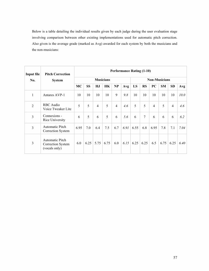
57

Below is a table detailing the individual results given by each judge during the user evaluation stage

involving comparison between other existing implementations used for automatic pitch correction.

Also given is the average grade (marked as Avg) awarded for each system by both the musicians and

the non-musicians:

Performance Rating (1-10)

Musicians Non-Musicians Input file

No.

Pitch Correction

System

MC SS HJ HK NP Avg LS RS PC SM SD Avg

1 Antares AVP-1 10 10 10 10 9 9.8 10 10 10 10 10 10.0

2 RBC Audio Voice Tweaker Lite

5 5 4 5 4 4.6 5 5 4 5 4 4.6

3 Connexions - Rice University

6 5 6 5 6 5.6 6 7 6 6 6 6.2

3 Automatic Pitch Correction System

6.95 7.0 6.4 7.5 6.7 6.91 6.55 6.8 6.95 7.8 7.1 7.04

3 Automatic Pitch Correction System (vocals only)

6.0 6.25 5.75 6.75 6.0 6.15 6.25 6.25 6.5 6.75 6.25 6.40