TECHNICAL REPORT 3026 December 2016

Auditory Weighting Functions and TTS/PTS Exposure Functions for

Marine Mammals Exposed to Underwater Noise

J. J. Finneran

Approved for public release. .

SSC Pacific San Diego, CA 92152-5001

SB

SSC SAN DIEGO San Diego, California 92152-5001

T. V. Flynn, CAPT, USN Commanding Officer

C. A. Keeney Executive Director

ADMINISTRATIVE INFORMATION This work described in this report was prepared for Commander, U.S. Fleet Forces Command,

Norfolk, VA, by the Marine Mammal Scientific & Vet Support Branch (Code 71510) of the Biosciences Division (Code 71500), Space and Naval Warfare Systems Center Pacific (SSC Pacific), San Diego, CA.

This is a work of the United States Government and therefore is not copyrighted. This work may be copied and disseminated without restriction. Many SSC San Diego public release documents are available in electronic format at http://www.spawar.navy.mil/sti/publications/pubs/index.html

Released under authority of M. J. Xitco, Head Biosciences Division

iii

EXECUTIVE SUMMARY

The U.S. Navy’s Tactical Training Theater Assessment and Planning (TAP) Program addresses environmental challenges that affect Navy training ranges and operating areas. As part of the TAP process, acoustic effects analyses are conducted to estimate the potential effects of Navy activities that introduce high-levels of sound or explosive energy into the marine environment. Acoustic effects analyses begin with mathematical modeling to predict the sound transmission patterns from Navy sources. These data are then coupled with marine species distribution and abundance data to determine the sound levels likely to be received by various marine species. Finally, criteria and thresholds are applied to estimate the specific effects that animals exposed to Navy-generated sound may experience.

This document describes the rationale and steps used to define proposed numeric thresholds for predicting auditory effects on marine mammals exposed to active sonars, other (non-impulsive) active acoustic sources, explosives, pile driving, and air guns for Phase 3 of the TAP Program. Since the derivation of TAP Phase 2 acoustic criteria and thresholds, important new data have been obtained related to the effects of noise on marine mammal hearing. Therefore, for Phase 3, new criteria and thresholds for the onset of temporary and permanent hearing loss have been developed, following a consistent approach for all species of interest and utilizing all relevant, available data. The effects of noise frequency on hearing loss are incorporated by using auditory weighting functions to emphasize noise at frequencies where a species is more sensitive to noise and de-emphasize noise at frequencies where susceptibility is low.

Marine mammals were divided into six groups for analysis: low-frequency cetaceans (group LF: mysticetes), mid-frequency cetaceans (group MF: delphinids, beaked whales, sperm whales), high-frequency cetaceans (group HF: porpoises, river dolphins), sirenians (group SI: manatees), phocids in water (group PW: true seals), and otariids and other non-phocid marine carnivores in water (group OW: sea lions, walruses, otters, polar bears).

For each group, a frequency-dependent weighting function and numeric thresholds for the onset of temporary threshold shift (TTS) and permanent threshold shift (PTS) were derived from available data describing hearing abilities of and effects of noise on marine mammals. The resulting weighting function amplitudes are illustrated in Figure E-1; Table E-1 summarizes the parameters necessary to calculate the weighting function amplitudes. For Navy Phase 3 analyses, the onset of TTS is defined as a TTS of 6 dB measured approximately 4 min after exposure. PTS is assumed to occur from exposures resulting in 40 dB or more of TTS measured approximately 4 min after exposure. Exposures just sufficient to cause TTS or PTS are denoted as “TTS onset” or “PTS onset” exposures.

iv

Figure E-1. Navy Phase 3 weighting functions for all species groups. Parameters required to generate the functions are provided in Table E-1.

Table E-1. Summary of weighting function parameters and TTS/PTS thresholds. SEL thresholds are in dB re 1 μPa2s and peak SPL thresholds are in dB re 1 μPa.

Non-impulsive Impulse

TTS Threshold

PTS Threshold

TTS Threshold

PTS Threshold

Group a b f1

(kHz) f2

(kHz) C

(dB) SEL

(Weighted) SEL

(Weighted) SEL

(Unweighted)

Peak SPL

(Unweighted)

SEL (Weighted)

Peak SPL

(Unweighted)

LF 1 2 0.20 19 0.13 179 199 168 213 183 219

MF 1.6 2 8.8 110 1.20 178 198 170 224 185 230

HF 1.8 2 12 140 1.36 153 173 140 196 155 202

SI 1.8 2 4.3 25 2.62 186 206 175 220 190 226

OW 2 2 0.94 25 0.64 199 219 188 226 203 232

PW 1 2 1.9 30 0.75 181 201 170 212 185 218

To compare the Phase 3 weighting functions and TTS/PTS thresholds to those used in TAP Phase 2 analyses, both the weighting function shape and the weighted threshold values must be taken into account; the weighted thresholds by themselves only indicate the TTS/PTS threshold at the most susceptible frequency (based on the relevant weighting function). In contrast, the TTS/PTS exposure functions incorporate both the shape of the weighting function and the weighted threshold value, they provide the best means of comparing the frequency-dependent TTS/PTS thresholds for Phase 2 and 3. Figures E-2 and E-3 compare the TTS/PTS exposure functions for non-impulsive sounds (e.g., sonars) and impulsive sounds (e.g., explosions), respectively, used in TAP Phase 2 and Phase 3.

v

Figure E-2. TTS and PTS exposure functions for sonars and other (non-impulsive) active acoustic sources. Heavy solid lines—Navy Phase 3 TTS exposure functions (Table E-1). Thin solid lines — Navy Phase 3 PTS exposure functions (Table E-1). Dashed lines—Navy Phase 2 TTS exposure functions. Short dashed lines—Navy Phase 2 PTS exposure functions.

vi

Figure E-3. TTS and PTS exposure functions for explosives, impact pile driving, air guns, and other impulsive sources. Heavy solid lines—Navy Phase 3 TTS exposure functions (Table E-1). Thin solid lines—Navy Phase 3 PTS exposure functions (Table E-1). Dashed lines—Navy Phase 2 TTS exposure functions. Short dashed lines—Navy Phase 2 PTS exposure functions.

The most significant differences between the Phase 2 and Phase 3 functions include: (1) Thresholds at low frequencies are generally higher for Phase 3 compared to Phase 2. This is because the Phase 2 weighting functions utilized the “M-weighting” functions at lower frequencies, where no TTS existed at that time. Since derivation of the Phase 2 weighting functions, additional data have been collected to support the use of new functions more similar to human auditory weighting functions. (2) Impulsive TTS/PTS thresholds near the region of best hearing sensitivity are lower for Phase 3 compared to Phase 2.

vii

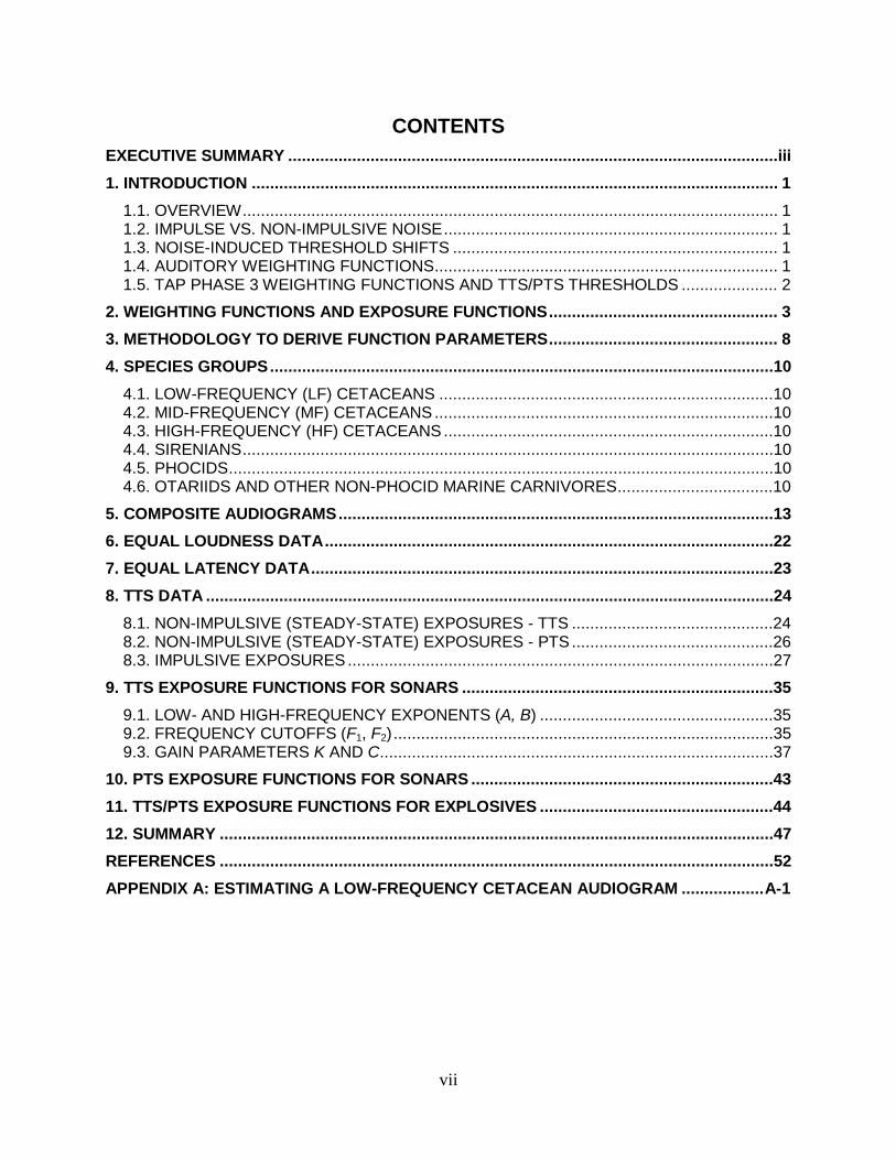
CONTENTS EXECUTIVE SUMMARY ...........................................................................................................iii 1. INTRODUCTION ................................................................................................................... 1

1.1. OVERVIEW ..................................................................................................................... 1 1.2. IMPULSE VS. NON-IMPULSIVE NOISE ......................................................................... 1 1.3. NOISE-INDUCED THRESHOLD SHIFTS ....................................................................... 1 1.4. AUDITORY WEIGHTING FUNCTIONS ........................................................................... 1 1.5. TAP PHASE 3 WEIGHTING FUNCTIONS AND TTS/PTS THRESHOLDS ..................... 2

2. WEIGHTING FUNCTIONS AND EXPOSURE FUNCTIONS .................................................. 33. METHODOLOGY TO DERIVE FUNCTION PARAMETERS .................................................. 84. SPECIES GROUPS ..............................................................................................................10

4.1. LOW-FREQUENCY (LF) CETACEANS .........................................................................10 4.2. MID-FREQUENCY (MF) CETACEANS ..........................................................................10 4.3. HIGH-FREQUENCY (HF) CETACEANS ........................................................................10 4.4. SIRENIANS ....................................................................................................................10 4.5. PHOCIDS .......................................................................................................................10 4.6. OTARIIDS AND OTHER NON-PHOCID MARINE CARNIVORES ..................................10

5. COMPOSITE AUDIOGRAMS ...............................................................................................136. EQUAL LOUDNESS DATA ..................................................................................................227. EQUAL LATENCY DATA .....................................................................................................238. TTS DATA ............................................................................................................................24

8.1. NON-IMPULSIVE (STEADY-STATE) EXPOSURES - TTS ............................................24 8.2. NON-IMPULSIVE (STEADY-STATE) EXPOSURES - PTS ............................................26 8.3. IMPULSIVE EXPOSURES .............................................................................................27

9. TTS EXPOSURE FUNCTIONS FOR SONARS ....................................................................359.1. LOW- AND HIGH-FREQUENCY EXPONENTS (A, B) ...................................................35 9.2. FREQUENCY CUTOFFS (F1, F2) ...................................................................................35 9.3. GAIN PARAMETERS K AND C ......................................................................................37

10. PTS EXPOSURE FUNCTIONS FOR SONARS ..................................................................4311. TTS/PTS EXPOSURE FUNCTIONS FOR EXPLOSIVES ...................................................4412. SUMMARY .........................................................................................................................47REFERENCES .........................................................................................................................52

APPENDIX A: ESTIMATING A LOW-FREQUENCY CETACEAN AUDIOGRAM .................. A-1

viii

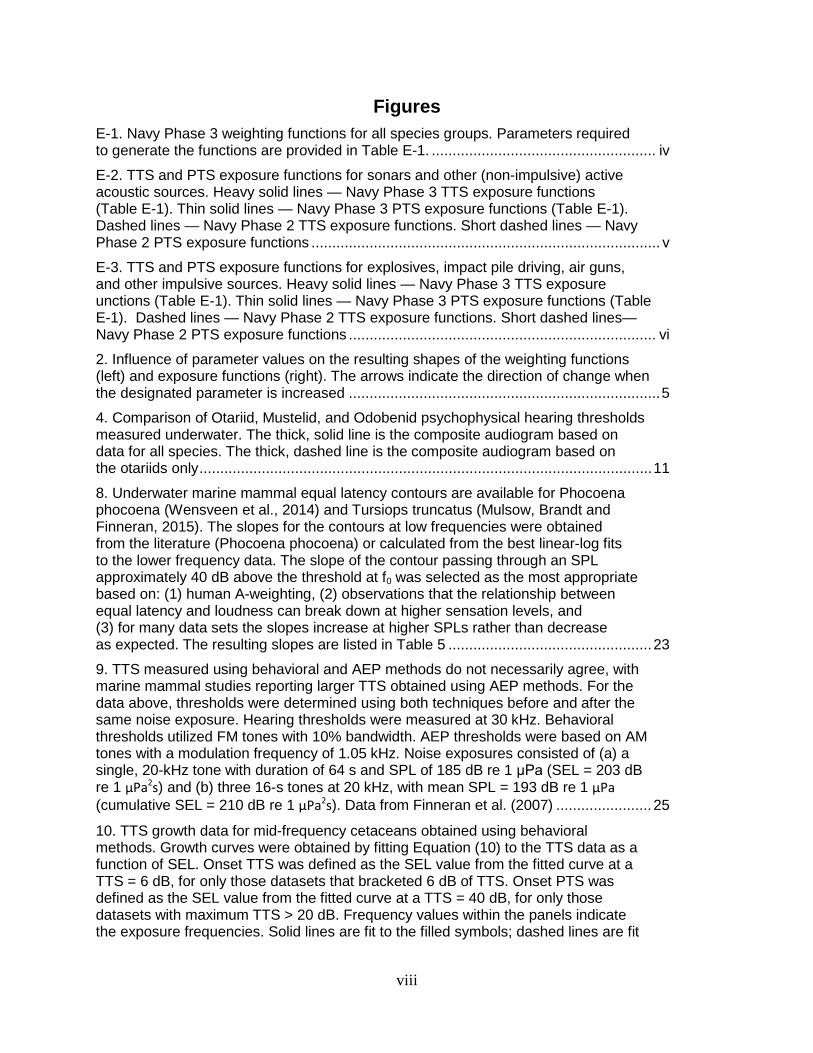
Figures E-1. Navy Phase 3 weighting functions for all species groups. Parameters required to generate the functions are provided in Table E-1. ...................................................... iv

E-2. TTS and PTS exposure functions for sonars and other (non-impulsive) active acoustic sources. Heavy solid lines — Navy Phase 3 TTS exposure functions (Table E-1). Thin solid lines — Navy Phase 3 PTS exposure functions (Table E-1). Dashed lines — Navy Phase 2 TTS exposure functions. Short dashed lines — Navy Phase 2 PTS exposure functions .................................................................................... v

E-3. TTS and PTS exposure functions for explosives, impact pile driving, air guns, and other impulsive sources. Heavy solid lines — Navy Phase 3 TTS exposure unctions (Table E-1). Thin solid lines — Navy Phase 3 PTS exposure functions (Table E-1). Dashed lines — Navy Phase 2 TTS exposure functions. Short dashed lines— Navy Phase 2 PTS exposure functions .......................................................................... vi

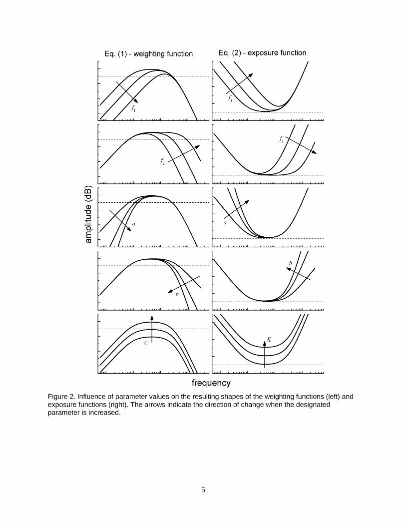
2. Influence of parameter values on the resulting shapes of the weighting functions(left) and exposure functions (right). The arrows indicate the direction of change when the designated parameter is increased ........................................................................... 5

4. Comparison of Otariid, Mustelid, and Odobenid psychophysical hearing thresholdsmeasured underwater. The thick, solid line is the composite audiogram based on data for all species. The thick, dashed line is the composite audiogram based on the otariids only ............................................................................................................. 11

8. Underwater marine mammal equal latency contours are available for Phocoenaphocoena (Wensveen et al., 2014) and Tursiops truncatus (Mulsow, Brandt and Finneran, 2015). The slopes for the contours at low frequencies were obtained from the literature (Phocoena phocoena) or calculated from the best linear-log fits to the lower frequency data. The slope of the contour passing through an SPL approximately 40 dB above the threshold at f0 was selected as the most appropriate based on: (1) human A-weighting, (2) observations that the relationship between equal latency and loudness can break down at higher sensation levels, and (3) for many data sets the slopes increase at higher SPLs rather than decrease as expected. The resulting slopes are listed in Table 5 ................................................. 23

9. TTS measured using behavioral and AEP methods do not necessarily agree, withmarine mammal studies reporting larger TTS obtained using AEP methods. For the data above, thresholds were determined using both techniques before and after the same noise exposure. Hearing thresholds were measured at 30 kHz. Behavioral thresholds utilized FM tones with 10% bandwidth. AEP thresholds were based on AM tones with a modulation frequency of 1.05 kHz. Noise exposures consisted of (a) a single, 20-kHz tone with duration of 64 s and SPL of 185 dB re 1 μPa (SEL = 203 dB re 1 μPa2s) and (b) three 16-s tones at 20 kHz, with mean SPL = 193 dB re 1 μPa (cumulative SEL = 210 dB re 1 μPa2s). Data from Finneran et al. (2007) ....................... 25

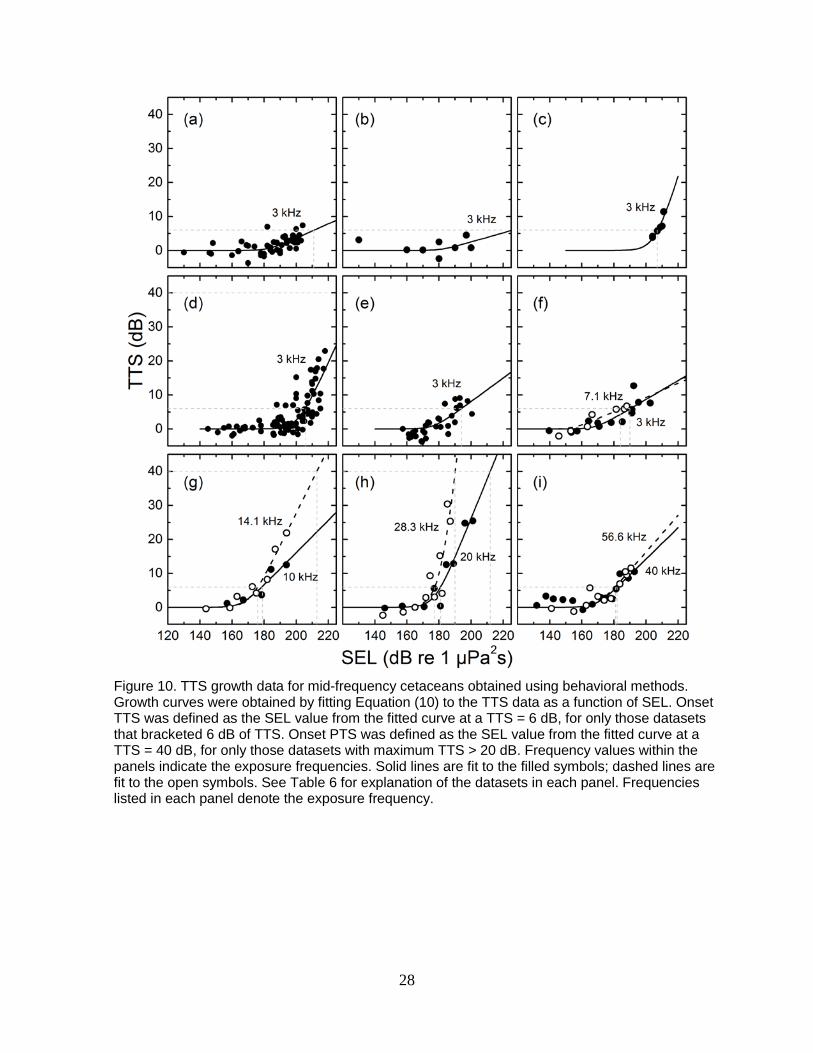
10. TTS growth data for mid-frequency cetaceans obtained using behavioralmethods. Growth curves were obtained by fitting Equation (10) to the TTS data as a function of SEL. Onset TTS was defined as the SEL value from the fitted curve at a TTS = 6 dB, for only those datasets that bracketed 6 dB of TTS. Onset PTS was defined as the SEL value from the fitted curve at a TTS = 40 dB, for only those datasets with maximum TTS > 20 dB. Frequency values within the panels indicate the exposure frequencies. Solid lines are fit to the filled symbols; dashed lines are fit

ix

to the open symbols. See Table 6 for explanation of the datasets in each panel. Frequencies listed in each panel denote the exposure frequency ................................. 28

11. TTS growth data for mid-frequency cetaceans obtained using AEP methods.Growth curves were obtained by fitting Equation (10) to the TTS data as a function of SEL. Onset TTS was defined as the SEL value from the fitted curve at a TTS = 6 dB, for only those datasets that bracketed 6 dB of TTS. Onset PTS was defined as the SEL value from the fitted curve at a TTS = 40 dB, for only those datasets with maximum TTS > 20 dB. Frequency values within the panels indicate the exposure frequencies. Solid lines are fit to the filled symbols; dashed lines are fit to the open symbols. See Table 6 for explanation of the datasets in each panel ............................. 29

12. TTS growth data for high-frequency cetaceans obtained using behavioral andAEP methods. Growth curves were obtained by fitting Equation (10) to the TTS data as a function of SEL. Onset TTS was defined as the SEL value from the fitted curve at a TTS = 6 dB, for only those datasets that bracketed 6 dB of TTS. Onset PTS was defined as the SEL value from the fitted curve at a TTS = 40 dB, for only those datasets with maximum TTS > 20 dB. The exposure frequency is specified in normal font; italics indicate the hearing test frequency. Percentages in panels (b), (d) indicate exposure duty cycle (duty cycle was 100% for all others). Solid lines are fit to the filled symbols; dashed lines are fit to the open symbols. See Table 6 for explanation of the datasets in each panel ..................................................................... 30

13. TS growth data for pinnipeds obtained using behavioral methods. Growth curveswere obtained by fitting Equation (10) to the TTS data as a function of SEL. Onset TTS was defined as the SEL value from the fitted curve at a TTS = 6 dB, for only those datasets that bracketed 6 dB of TTS. Frequency values within the panels indicate the exposure frequencies. Numeric values in panel (c) indicate subjects 01 and 02. Solid lines are fit to the filled symbols; dashed lines are fit to the open symbols. See Table 6 for explanation of the datasets in each panel ............................. 31

14. The cutoff frequencies f1 and f2 were defined as the frequencies below and abovef0 at which the composite audiogram values were ∆T-dB above the threshold at f0 (the lowest threshold) ........................................................................................................... 36

15. Effect of ∆T adjustment on the TTS exposure functions for the mid-frequencycetaceans (left) and high-frequency cetaceans (right). To calculate the exposure functions, a and b were defined as a = s0/20 and b = 2. ∆T was then varied from 0 to 20. At each value of ∆T, K was adjusted to minimize the squared error between the exposure function and the onset TTS data (symbols). As ∆T increases, f1 decreases and f2 increases, causing the pass-band of the function to increase and the function to “flatten” .................................................................................................. 36

16. Relationship between ∆T and the resulting mean-squared error (MSE) betweenthe exposure functions and onset TTS data. The MSE was calculated by adding the squared errors between the exposure functions and TTS data for the MF and HF cetacean groups, then dividing by the total number of TTS data points. This process was performed using the composite audiograms based on original and normalized threshold data and ∆T values from 0 to 20. The lowest MSE value was obtained using the audiograms based on normalized thresholds with ∆T = 9 dB (arrow) ............. 37

17. Exposure functions (solid lines) generated from Equation (2) with the parametersspecified in Table 7. Dashed lines — (normalized) composite audiograms used for definition of parameters a, f1, and f2. A constant value was added to each

x

audiogram to equate the minimum audiogram value with the exposure function minimum. Short dashed line — Navy Phase 2 exposure functions for TTS onset for each group. Filled symbols — onset TTS exposure data (in dB SEL) used to define exposure function shape and vertical position. Open symbols — estimated TTS onset for species for which no TTS data exist .............................................................................. 39

18. Mid-frequency cetacean exposure function, (normalized) composite audiogram,and Phase 2 exposure functions compared to mid-frequency cetacean TTS data. Large symbols with no numeric values indicate onset TTS exposures. Smaller symbols represent specific amounts of TTS observed, with numeric values giving the amount (or range) or measured TTS. Filled and half-filled symbols — behavioral data. Open symbols — AEP data .................................................................................................... 40

19. High-frequency cetacean TTS exposure function, (normalized) compositeaudiogram, and Phase 2 exposure functions compared to high-frequency cetacean TTS data. Large symbols with no numeric values indicate onset TTS exposures. Smaller symbols represent specific amounts of TTS observed, with numeric values giving the amount (or range) or measured TTS. Filled and half-filled symbols — behavioral data. Open symbols — AEP data ................................................................ 41

20. Phocid (underwater) exposure function, (normalized) composite audiogram, andPhase 2 exposure functions compared to phocid TTS data. Large symbols with no numeric values indicate onset TTS exposures. Smaller symbols represent specific amounts of TTS observed, with numeric values giving the amount (or range) or measured TTS .............................................................................................................. 42

21. Navy Phase 3 weighting functions for marine mammal species groups exposedto underwater sound. Parameters required to generate the functions are provided in Table 10 ........................................................................................................................ 47

22. TTS and PTS exposure functions for sonars and other (non-impulsive) activeacoustic sources. Heavy solid lines — Navy Phase 3 TTS exposure functions (Table 10). Thin solid lines — Navy Phase 3 PTS exposure functions for TTS (Table 10). Dashed lines — Navy Phase 2 TTS exposure functions. Short dashed lines — Navy Phase 2 PTS exposure functions. ........................................................................ 50

23. TTS and PTS exposure functions for explosives, impact pile driving, air guns, andother impulsive sources. Heavy solid lines — Navy Phase 3 TTS exposure functions (Table 10). Thin solid lines — Navy Phase 3 PTS exposure functions for TTS (Table 10). Dashed lines — Navy Phase 2 TTS exposure functions. Short dashed lines — Navy Phase 2 PTS exposure functions ......................................................................... 51

A-1. Relationship between estimated threshold, T(f): thick gray line, low-frequency term, L(f): solid line, and high-frequency term, H(f): dashed line ..................................... 4

A-2. Comparison of proposed LF cetacean thresholds to those predicted by anatomical and finite-element models ............................................................................. 6

xi

Tables E-1. Summary of weighting function parameters and TTS/PTS thresholds. SEL thresholds

are in dB re 1 μPa2s and peak SPL thresholds are in dB re 1 μPa ..................................... iv

1. Species group designations for Navy Phase 3 auditory weighting functions ..........................12

2. References, species, and individual subjects used to derive the composite audiograms .......15

3. Composite audiogram parameters values for use in Equation (9). For all groups exceptLF cetaceans, values represent the best-fit parameters from fitting Equation (9) to experimental threshold data. For the low-frequency cetaceans, parameter values for Equation (9) were estimated as described in Appendix A .............................................17

4. Normalized composite audiogram parameters values for use in Equation (9). For allgroups except LF cetaceans, values represent the best-fit parameters after fitting Equation (9) to normalized threshold data. For the low-frequency cetaceans, parameter values for Equation (9) were estimated as described in Appendix A .................17

5. Frequency of best hearing ( f0) and the magnitude of the low-frequency slope (s0)derived from composite audiograms and equal latency contours. For the species with composite audiograms based on experimental data (i.e., all except LF cetaceans), audiogram slopes were calculated across a frequency range of one decade beginning with the lowest frequency present for each group. The low-frequency slope for LF cetaceans was not based on a curve-fit but explicitly defined during audiogram derivation (see Appendix A). Equal latency slopes were calculated from the available equal latency contours (Figure 8) ......................................................................................21

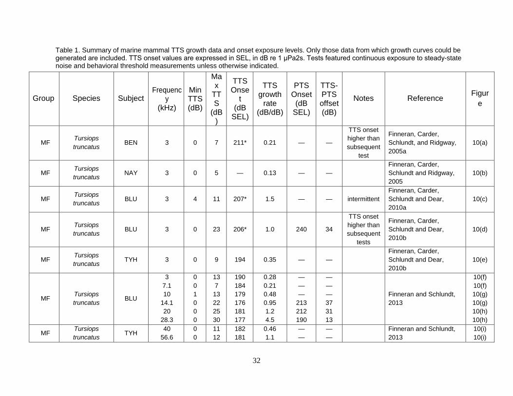
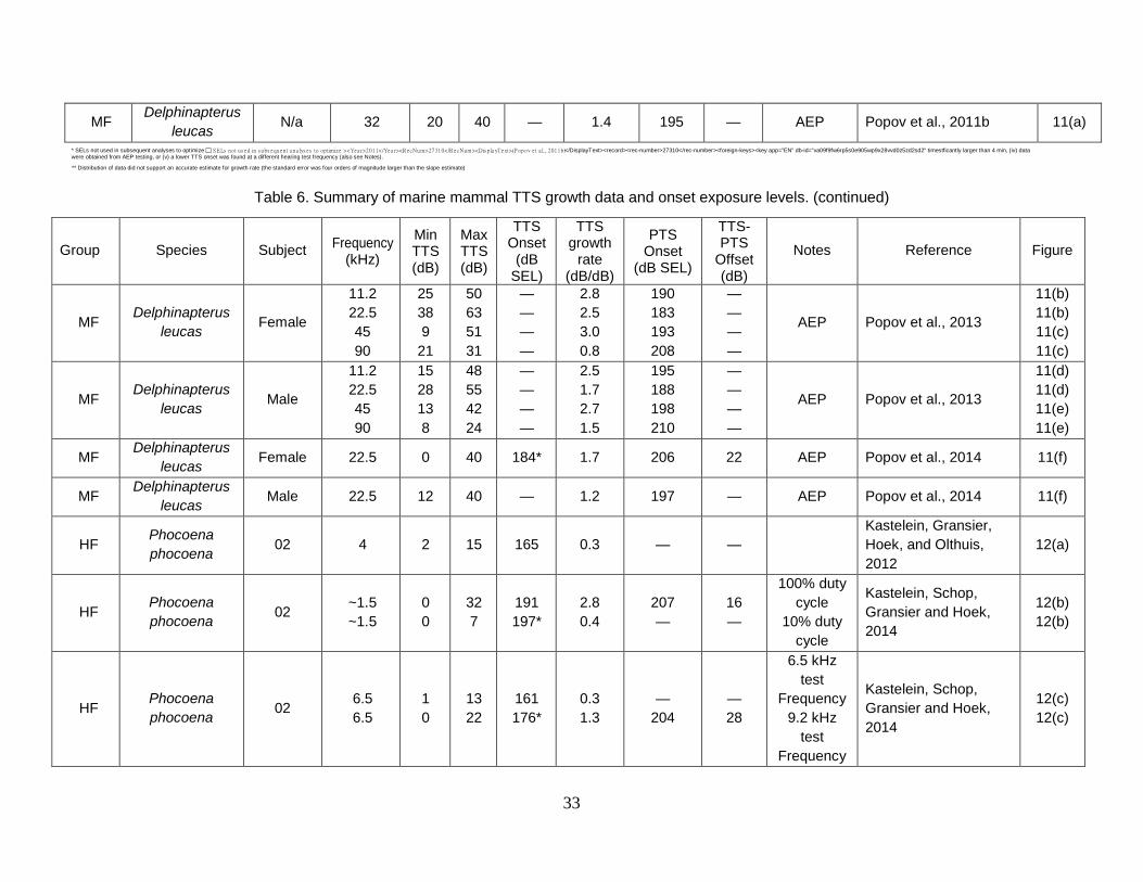
6. Summary of marine mammal TTS growth data and onset exposure levels. Only thosedata from which growth curves could be generated are included. TTS onset values are expressed in SEL, in dB re 1 μPa2s. Tests featured continuous exposure to steady-state noise and behavioral threshold measurements unless otherwise indicated ............................................................................................................................32

7. Differences between composite threshold values (Figure 5) and TTS onset values at thefrequency of best hearing (f0) for the in-water marine mammal species groups. The values for the low-frequency cetaceans and sirenians were estimated using the median difference (126) from the MF, HF, OW, and PW groups ....................................................38

8. Weighting function and TTS exposure function parameters for use in Equations (1) and(2) for steady-state exposures. R2 values represent goodness of fit between exposure function and TTS onset data (Table 6) ..............................................................................38

9. TTS and PTS thresholds for explosives and other impulsive sources. SEL thresholdsare in dB re 1 μPa2s and peak SPL thresholds are in dB re 1 μPa ....................................46

10. Summary of weighting function parameters and TTS/PTS thresholds. SEL thresholdsare in dB re 1 μPa2s and peak SPL thresholds are in dB re 1 μPa ....................................48

A-1. Sample table ................................................................................................................... A-6

1

1. INTRODUCTION1.1. OVERVIEW

The U.S. Navy’s Tactical Training Theater Assessment and Planning (TAP) Program addresses environmental challenges that affect Navy training ranges and operating areas. As part of the TAP process, acoustic effects analyses are conducted to estimate the potential effects of Navy training and testing activities that introduce high-levels of sound or explosive energy into the marine environment. Acoustic effects analyses begin with mathematical modeling to predict the sound transmission patterns from Navy sources. These data are then coupled with marine species distribution and abundance data to determine sound levels likely to be received by various marine species. Finally, criteria and thresholds are applied to estimate the specific effects that animals exposed to Navy-generated sound may experience.

This document describes the rationale and steps used to define proposed numeric thresholds for predicting auditory effects on marine mammals exposed to underwater sound from active sonars, other (non-impulsive) active acoustic sources, explosives, pile driving, and air guns for Phase 3 of the TAP Program. The weighted threshold values and auditory weighting function shapes are summarized in Section 12. 1.2. IMPULSE VS. NON-IMPULSIVE NOISE

When analyzing the auditory effects of noise exposure, it is often helpful to broadly categorize noise as either impulse noise—noise with high peak sound pressure, short duration, fast rise-time, and broad frequency content—or non-impulsive (i.e., steady-state) noise. When considering auditory effects, sonars, other coherent active sources, and vibratory pile driving are considered to be non-impulsive sources, while explosives, impact pile driving, and air guns are treated as impulsive sources. Note that the terms non-impulsive or steady-state do not necessarily imply long duration signals, only that the acoustic signal has sufficient duration to overcome starting transients and reach a steady-state condition. For harmonic signals, sounds with duration greater than approximately 5 to 10 cycles are generally considered steady-state. 1.3. NOISE-INDUCED THRESHOLD SHIFTS

Exposure to sound with sufficient duration and sound pressure level (SPL) may result in an elevated hearing threshold (i.e., a loss of hearing sensitivity), called a noise-induced threshold shift (NITS). If the hearing threshold eventually returns to normal, the NITS is called a temporary threshold shift (TTS); otherwise, if thresholds remain elevated after some extended period of time, the remaining NITS is called a permanent threshold shift (PTS). TTS and PTS data have been used to guide the development of safe exposure guidelines for people working in noisy environments. Similarly, TTS and PTS criteria and thresholds form the cornerstone of Navy analyses to predict auditory effects in marine mammals incidentally exposed to intense underwater sound during naval activities. 1.4. AUDITORY WEIGHTING FUNCTIONS

Animals are not equally sensitive to noise at all frequencies. To capture the frequency-dependent nature of the effects of noise, auditory weighting functions are used. Auditory weighting functions are mathematical functions used to emphasize frequencies where animals are more susceptible to noise exposure and de-emphasize frequencies where animals are less susceptible. The functions may be thought of as frequency-dependent filters that are applied to a noise exposure before a single, weighted SPL or sound exposure level (SEL) is calculated. The filter shapes are normally “band-pass” in nature; i.e., the function amplitude resembles an inverted “U” when plotted versus

2

frequency. The weighting function amplitude is approximately flat within a limited range of frequencies, called the “pass-band,” and declines at frequencies below and above the pass-band.

Auditory weighting functions for humans were based on equal loudness contours—curves that show the combinations of SPL and frequency that result in a sensation of equal loudness in a human listener. Equal loudness contours are in turn created from data collected during loudness comparison tasks. Analogous tasks are difficult to perform with non-verbal animals; as a result, equal loudness contours are available for only a single marine mammal (a dolphin) across a limited range of frequencies (2.5 to 113 kHz) (Finneran and Schlundt, 2011). In lieu of performing loudness comparison tests, reaction times to tones can be measured, under the assumption that reaction time is correlated with subjective loudness (Stebbins, 1966; Pfingst, Heinz, Kimm, and Miller, 1975). From the reaction time vs. SPL data, curves of equal response latency can be created and used as proxies for equal loudness contours.

Just as human damage risk criteria use auditory weighting functions to capture the frequency-dependent aspects of noise, U.S. Navy acoustic impact analyses use weighting functions to capture the frequency-dependency of TTS and PTS in marine mammals. 1.5. TAP PHASE 3 WEIGHTING FUNCTIONS AND TTS/PTS THRESHOLDS

Navy weighting functions for TAP Phase 2 (Finneran and Jenkins, 2012) were based on the “M-weighting” curves defined by Southall et al. (2007), with additional high-frequency emphasis for cetaceans based on equal loudness contours for a bottlenose dolphin (Finneran and Schlundt, 2011). Phase 2 TTS/PTS thresholds also relied heavily on the recommendations of Southall et al. (2007), with modifications based on preliminary data for the effects of exposure frequency on dolphin TTS (Finneran, 2010; Finneran and Schlundt, 2010) and limited TTS data for harbor porpoises (Lucke, Siebert, Lepper, and Blanchet, 2009; Kastelein et al., 2011).

Since the derivation of TAP Phase 2 acoustic criteria and thresholds, new data have been obtained regarding marine mammal hearing (e.g., Piniak, Eckert, Harms and Stringer, 2012; Martin et al., 2012; Ghoul and Reichmuth, 2014; Sills, Southall and Reichmuth, 2014; Sills, Southall and Reichmuth, 2015), marine mammal equal latency contours (e.g., Reichmuth, 2013; Wensveen, Huijser, Hoek and Kastelein, 2014; Mulsow, Schlundt, Brandt and Finneran, 2015), and the effects of noise on marine mammal hearing (e.g., Kastelein et al., 2012; Kastelein, Gransier, Hoek and Olthuis, 2012; Finneran and Schlundt, 2013; Kastelein, Gransier and Hoek, 2013; Kastelein, Gransier, Hoek and Rambags, 2013; Popov et al., 2013; Kastelein et al., 2014; Kastelein, Schop, Gransier and Hoek, 2014; Popov et al., 2014; Finneran et al., 2015; Kastelein, Gransier, Marijt and Hoek, 2015; Kastelein, Gransier, Schop and Hoek, 2015; Popov et al., 2015) As a result, new weighting functions and TTS/PTS thresholds have been developed for Phase 3. The new criteria and thresholds are based on all relevant data and feature a consistent approach for all species of interest.

Marine mammals were divided into six groups for analysis. For each group, a frequency-dependent weighting function and numeric thresholds for the onset of TTS and PTS were derived from available data describing hearing abilities and effects of noise on marine mammals. Measured or predicted auditory threshold data, as well as measured equal latency contours, were used to influence the weighting function shape for each group. For species groups for which TTS data are available, the weighting function parameters were adjusted to provide the best fit to the experimental data. The same methods were then applied to other groups for which TTS data did not exist.

3

2. WEIGHTING FUNCTIONS AND EXPOSURE FUNCTIONSThe shapes of the Phase 3 auditory weighting functions are based on a generic band-pass filter

described by

, (1)

where W( f ) is the weighting function amplitude (in dB) at the frequency f (in kHz). The shape of the filter is defined by the parameters C, f1, f2, a, and b (Figures 1 and 2, left panels):

C weighting function gain (dB). The value of C defines the vertical position of the curve. Changing the value of C shifts the function up/down. The value of C is often chosen to set the maximum amplitude of W to 0 dB (i.e., the value of C does not necessarily equal the peak amplitude of the curve).

f1 low-frequency cutoff (kHz). The value of f1 defines the lower limit of the filter pass-band; i.e., the lower frequency at which the weighting function amplitude begins to decline or“roll-off” from the flat, central portion of the curve. The specific amplitude at f1 depends on the value of a. Decreasing f1 will enlarge the pass-band of the function (the flat, central portion of the curve).

f2 high-frequency cutoff (kHz). The value of f2 defines the upper limit of the filter pass-band; i.e., the upper frequency at which the weighting function amplitude begins to roll-off from the flat, central portion of the curve. The amplitude at f2 depends on the value of b. Increasing f2 will enlarge the pass-band of the function.

a low-frequency exponent (dimensionless). The value of a defines the rate at which the weighting function amplitude declines with frequency at the lower frequencies. As frequency decreases, the change in weighting function amplitude becomes linear with the logarithm of frequency, with a slope of 20a dB/decade. Larger values of a result in lower amplitudes at f1 and steeper rolloffs at frequencies below f1.

b high-frequency exponent (dimensionless). The value of b defines the rate at which the weighting function amplitude declines with frequency at the upper frequencies. As frequency increases, the change in weighting function amplitude becomes linear with the logarithm of frequency, with a slope of -20b dB/decade. Larger values of b result in lower amplitudes at f2 and steeper rolloffs at frequencies above f2.

If a = 2 and b = 2, Equation (1) is equivalent to the functions used to define Navy Phase 2 Type I and EQL weighting functions, M-weighting functions, and the human C-weighting function (American National Standards Institute (ANSI), 2001; Southall et al., 2007; Finneran and Jenkins, 2012). The change from fixed to variable exponents for Phase 3 was done to allow the low- and high-frequency rolloffs to match available experimental data. During implementation, the weighting function defined by Equation (1) is used in conjunction with a weighted threshold for TTS or PTS expressed in units of SEL.

4

Figure 1. Examples of (left) weighting function amplitude described by Equation (1) and (right) exposure function described by Equation (2). The parameters f1 and f2 specify the extent of the filter pass-band, while the exponents a and b control the rate of amplitude change below f1 and above f2, respectively. As the frequency decreases below f1 or above f2, the amplitude approaches linear-log behavior with a slope magnitude of 20a or 20b dB/decade, respectively. The constants C and K determine the vertical positions of the curves.

5

Figure 2. Influence of parameter values on the resulting shapes of the weighting functions (left) and exposure functions (right). The arrows indicate the direction of change when the designated parameter is increased.

6

For developing and visualizing the effects of the various weighting functions, it is helpful to invert Equation (1), yielding

, (2)

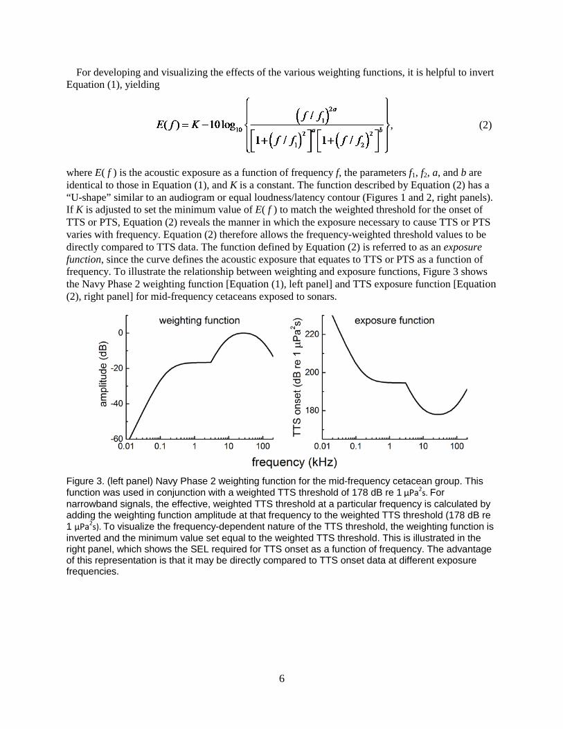
where E( f ) is the acoustic exposure as a function of frequency f, the parameters f1, f2, a, and b are identical to those in Equation (1), and K is a constant. The function described by Equation (2) has a “U-shape” similar to an audiogram or equal loudness/latency contour (Figures 1 and 2, right panels). If K is adjusted to set the minimum value of E( f ) to match the weighted threshold for the onset of TTS or PTS, Equation (2) reveals the manner in which the exposure necessary to cause TTS or PTS varies with frequency. Equation (2) therefore allows the frequency-weighted threshold values to be directly compared to TTS data. The function defined by Equation (2) is referred to as an exposure function, since the curve defines the acoustic exposure that equates to TTS or PTS as a function of frequency. To illustrate the relationship between weighting and exposure functions, Figure 3 shows the Navy Phase 2 weighting function [Equation (1), left panel] and TTS exposure function [Equation (2), right panel] for mid-frequency cetaceans exposed to sonars.

Figure 3. (left panel) Navy Phase 2 weighting function for the mid-frequency cetacean group. This function was used in conjunction with a weighted TTS threshold of 178 dB re 1 μPa2s. For narrowband signals, the effective, weighted TTS threshold at a particular frequency is calculated by adding the weighting function amplitude at that frequency to the weighted TTS threshold (178 dB re 1 μPa2s). To visualize the frequency-dependent nature of the TTS threshold, the weighting function is inverted and the minimum value set equal to the weighted TTS threshold. This is illustrated in the right panel, which shows the SEL required for TTS onset as a function of frequency. The advantage of this representation is that it may be directly compared to TTS onset data at different exposure frequencies.

7

The relationships between Equations (1) and (2) may be highlighted by defining the function X( f ) as

. (3)

The peak value of X( f ) depends on the specific values of f1, f2, a, and b and will not necessarily equal zero. Substituting Equation (3) into Equations (1) and (2) results in

(4)

and

, (5)

respectively. The maximum of the weighting function and the minimum of the exposure function occur at the same frequency, denoted fp. The constant C is defined so the weighting function maximum value is 0 dB; i.e., W( fp ) = 0, so

. (6)

The constant K is defined so that the minimum of the exposure function [i.e., the value of E( f ) when f = fp ] equals the weighted TTS or PTS threshold, Twgt, so

. (7)

Adding Equations (6) and (7) results in

. (8)

The constants C, K, and the weighted threshold are therefore not independent and any one of these parameters can be calculated if the other two are known.

8

3. METHODOLOGY TO DERIVE FUNCTION PARAMETERS Weighting and exposure functions are defined by selecting appropriate values for the parameters

C, K, f1, f2, a, and b in Equations (1) and (2). Ideally, these parameters would be based on experimental data describing the manner in which the onset of TTS or PTS varied as a function of exposure frequency. In other words, a weighting function for TTS should ideally be based on TTS data obtained using a range of exposure frequencies, species, and individual subjects within each species group. However, currently there are only limited data for the frequency-dependency of TTS in marine mammals. Therefore, weighting and exposure function derivations relied upon auditory threshold measurements (audiograms), equal latency contours, anatomical data, and TTS data when available.

Although the weighting function shapes are heavily influenced by the shape of the auditory sensitivity curve, the two are not identical. Essentially, the auditory sensitivity curves are adjusted to match the existing TTS data in the frequency region near best sensitivity (step 4 below). This results in “compression” of the auditory sensitivity curve in the region near best sensitivity to allow the weighting function shape to match the TTS data, which show less change with frequency compared to hearing sensitivity curves in the frequency region near best sensitivity.

Weighting and exposure function derivation consisted of the following steps:

1. Marine mammals were divided into six groups based on auditory, ecological, and phylogenetic relationships among species.

2. For each species group, a representative, composite audiogram (a graph of hearing threshold vs. frequency) was estimated.

3. The exponent a was defined using the smaller of the low-frequency slope from the composite audiogram or the low-frequency slope of equal latency contours. The exponent b was set equal to two.

4. The frequencies f1 and f2 were defined as the frequencies at which the composite threshold values are ΔT-dB above the lowest threshold value. The value of ΔT was chosen to minimize the mean-squared error between Equation (2) and the non-impulsive TTS data for the mid- and high-frequency cetacean groups.

5. For species groups for which TTS onset data exist, K was adjusted to minimize the squared error between Equation (2) and the steady-state (non-impulsive) TTS onset data. For other species, K was defined to provide the best estimate for TTS onset at a representative frequency. The minimum value of the TTS exposure function (which is not necessarily equal to K) was then defined as the weighted TTS threshold.

6. The constant C was defined to set the peak amplitude of the function defined by Equation (1) to zero. This is mathematically equivalent to setting C equal to the difference between the weighted threshold and K [see Equation (8)].

7. The weighted threshold for PTS was derived for each group by adding a constant value (20 dB) to the weighted TTS thresholds. The constant was based on estimates of the difference in exposure levels between TTS onset and PTS onset (i.e., 40 dB of TTS) obtained from the marine mammal TTS growth curves.

9

8. For the mid- and high-frequency cetaceans, weighted TTS and PTS thresholds for explosives and other impulsive sources were obtained from the available impulse TTS data. For other groups, the weighted SEL thresholds were estimated using the relationship between the steady-state TTS weighted threshold and the impulse TTS weighted threshold for the mid- and high-frequency cetaceans. Peak SPL thresholds were estimated using the relationship between hearing thresholds and the impulse TTS peak SPL thresholds for the mid- and high-frequency cetaceans.

The remainder of this report addresses these steps in detail.

 

10

4. SPECIES GROUPS

Marine mammals were divided into six groups (Table 1), with the same weighting function and TTS/PTS thresholds used for all species within a group. Species were grouped by considering their known or suspected audible frequency range, auditory sensitivity, ear anatomy, and acoustic ecology (i.e., how they use sound), as has been done previously (e.g., Ketten, 2000; Southall et al., 2007; Finneran and Jenkins, 2012). 4.1. LOW-FREQUENCY (LF) CETACEANS

The LF cetacean group contains all of the mysticetes (baleen whales). Although there have been no direct measurements of hearing sensitivity in any mysticete, an audible frequency range of approximately 10 Hz to 30 kHz has been estimated from observed vocalization frequencies, observed reactions to playback of sounds, and anatomical analyses of the auditory system. A natural division may exist within the mysticetes, with some species (e.g., blue, fin) having better low-frequency sensitivity and others (e.g., humpback, minke) having better sensitivity to higher frequencies; however, at present there is insufficient knowledge to justify separating species into multiple groups. Therefore, a single species group is used for all mysticetes. 4.2. MID-FREQUENCY (MF) CETACEANS

The MF cetacean group contains most delphinid species (e.g., bottlenose dolphin, common dolphin, killer whale, pilot whale), beaked whales, and sperm whales (but not pygmy and dwarf sperm whales of the genus Kogia, which are treated as high-frequency species). Hearing sensitivity has been directly measured for a number of species within this group using psychophysical (behavioral) or auditory evoked potential (AEP) measurements. 4.3. HIGH-FREQUENCY (HF) CETACEANS

The HF cetacean group contains the porpoises, river dolphins, pygmy/dwarf sperm whales, Cephalorhynchus species, and some Lagenorhynchus species. Hearing sensitivity has been measured for several species within this group using behavioral or AEP measurements. High-frequency cetaceans generally possess a higher upper-frequency limit and better sensitivity at high frequencies compared to the mid-frequency cetacean species. 4.4. SIRENIANS

The sirenian group contains manatees and dugongs. Behavioral and AEP threshold measurements for manatees have revealed lower upper cutoff frequencies and sensitivities compared to the mid-frequency cetaceans. 4.5. PHOCIDS

This group contains all earless seals or “true seals,” including all Arctic and Antarctic ice seals, harbor or common seals, gray seals and inland seals, elephant seals, and monk seals. Underwater hearing thresholds exist for some Northern Hemisphere species in this group. 4.6. OTARIIDS AND OTHER NON-PHOCID MARINE CARNIVORES

This group contains all eared seals (fur seals and sea lions), walruses, sea otters, and polar bears. The division of marine carnivores by placing phocids in one group and all others into a second group was made after considering auditory anatomy and measured audiograms for the various species and noting the similarities between the non-phocid audiograms (Figure 4). Underwater hearing thresholds exist for some Northern Hemisphere species in this group.

11

Figure 4. Comparison of Otariid, Mustelid, and Odobenid psychophysical hearing thresholds measured underwater. The thick, solid line is the composite audiogram based on data for all species. The thick, dashed line is the composite audiogram based on the otariids only.

12

Table 1. Species group designations for Navy Phase 3 auditory weighting functions.

Code Name Members

LF Low-frequency cetaceans

Family Balaenidae (right and bowhead whales) Family Balaenopteridae (rorquals) Family Eschrichtiidae (gray whale) Family Neobalaenidae (pygmy right whale)

MF Mid-frequency cetaceans

Family Ziphiidae (beaked whales) Family Physeteridae (Sperm whale) Family Monodontidae (Irrawaddy dolphin, beluga, narwhal) Subfamily Delphininae (white-beaked/white-sided/ Risso’s/bottlenose/spotted/spinner/striped/common dolphins) Subfamily Orcininae (melon-headed whales, false/pygmy killer whale, killer whale, pilot whales) Subfamily Stenoninae (rough-toothed/humpback dolphins) Genus Lissodelphis (right whale dolphins) Lagenorhynchus albirostris (white-beaked dolphin) Lagenorhynchus acutus (Atlantic white-sided dolphin) Lagenorhynchus obliquidens (Pacific white-sided dolphin) Lagenorhynchus obscurus (dusky dolphin)

HF High-frequency cetaceans

Family Phocoenidae (porpoises) Family Platanistidae (Indus/Ganges river dolphins) Family Iniidae (Amazon river dolphins) Family Pontoporiidae (Baiji/ La Plata river dolphins) Family Kogiidae (Pygmy/dwarf sperm whales) Genus Cephalorhynchus (Commersen’s, Chilean, Heaviside’s, Hector’s dolphins) Lagenorhynchus australis (Peale’s or black-chinned dolphin) Lagenorhynchus cruciger (hourglass dolphin)

SI Sirenians Family Trichechidae (manatees) Family Dugongidae (dugongs)

OW Otariids and other non-phocid marine carnivores (water)

Family Otariidae (eared seals and sea lions) Family Odobenidae (walrus) Enhydra lutris (sea otter) Ursus maritimus (polar bear)

PW Phocids (water) Family Phocidae (true seals)

 

13

5. COMPOSITE AUDIOGRAMS

Composite audiograms for each species group were determined by first searching the available literature for threshold data for the species of interest. For each group, all available AEP and psychophysical (behavioral) threshold data were initially examined. To derive the composite audiograms, the following rules were applied:

1. For species groups with three or more behavioral audiograms (all groups except LF cetaceans), only behavioral (no AEP) data were used. Mammalian AEP thresholds are typically elevated from behavioral thresholds in a frequency-dependent manner, with increasing discrepancy between AEP and behavioral thresholds at the lower frequencies where there is a loss of phase synchrony in the neurological responses and a concomitant increase in measured AEP thresholds. The frequency-dependent relationship between the AEP and behavioral data is problematic for defining the audiogram slope at low frequencies, since the AEP data will systematically over-estimate thresholds and therefore over-estimate the low-frequency slope of the audiogram. As a result of this rule, behavioral data were used for all marine mammal groups.

For the low-frequency cetaceans, for which no behavioral or AEP threshold data exist, hearing thresholds were estimated by synthesizing information from anatomical measurements, mathematical models of hearing, and animal vocalization frequencies (see Appendix A).

2. Data from an individual animal were included only once at a particular frequency. If data from the same individual were available from multiple studies, data at overlapping frequencies were averaged.

3. Individuals with obvious high-frequency hearing loss for their species or aberrant audiograms (e.g., obvious notches or thresholds known to be elevated for that species due to masking or hearing loss) were excluded.

4. Linear interpolation was performed within the threshold data for each individual to estimate a threshold value at each unique frequency present in any of the data for that species group. This was necessary to calculate descriptive statistics at each frequency without excluding data from any individual subject.

5. Composite audiograms were determined using both the original threshold values from each individual (in dB re 1 μPa) and normalized thresholds obtained by subtracting the lowest threshold value for that subject.

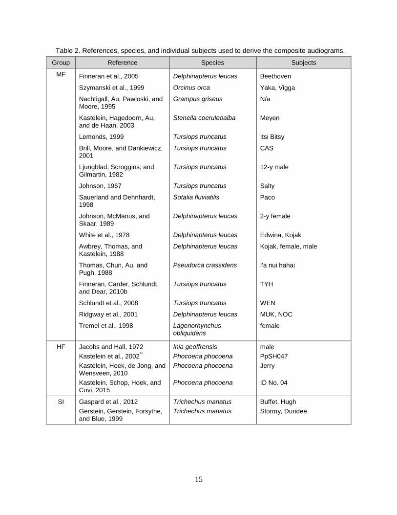
Table 2 lists the individual references for the data ultimately used to construct the composite audiograms (for all species groups except the LF cetaceans). From these data, the median (50th percentile) threshold value was calculated at each frequency and fit by the function

T ( f ) T0 A log10 1 F1

f

f

F2

B

, (9)

14

where T( f ) is the threshold at frequency f, and T0, F1, F2, A, and B are fitting parameters. The median value was used to reduce the influence of outliers. The particular form of Equation (9) was chosen to provide linear-log rolloff with variable slope at low frequencies and a steep rise at high frequencies. The form is similar to that used by Popov et al. (2007) to describe dolphin audiograms; the primary difference between the two is the inclusion of two frequency parameters in Equation (9), which allows a more shallow slope in the region of best sensitivity. Equation (9) was fit to the median threshold data using nonlinear regression (National Instruments LabVIEW 2015). The resulting fitting parameters and goodness of fit values (R2) are provided in Tables 3 and 4 for the original and normalized data, respectively. Equation (9) was also used to describe the shape of the estimated audiogram for the LF cetaceans, with the parameter values chosen to provide reasonable thresholds based on the limited available data regarding mysticete hearing (see Appendix A for details).

Figures 5 and 6 show the original and normalized threshold data, respectively, as well as the composite audiograms based on the fitted curve. The composite audiograms for each species group are compared in Figure 6. To allow comparison with other audiograms based on the original threshold data, the lowest threshold for the low-frequency cetaceans was estimated to be 54 dB re 1 μPa, based on the median of the thresholds for the other in-water species groups (MF, HF, SI, OW, PW). From the composite audiograms, the frequency of lowest threshold, f0, and the slope at the lower frequencies, s0, were calculated (Table 5). For the species with composite audiograms based on experimental data (i.e., all except LF cetaceans), audiogram slopes were calculated across a frequency range of one decade beginning with the lowest frequency present for each group. The low-frequency slope for LF cetaceans was not based on a curve-fit but explicitly defined during audiogram derivation (see Appendix A).

15

Table 2. References, species, and individual subjects used to derive the composite audiograms.

Group Reference Species Subjects

MF Finneran et al., 2005

Szymanski et al., 1999

Nachtigall, Au, Pawloski, and Moore, 1995

Kastelein, Hagedoorn, Au, and de Haan, 2003

Lemonds, 1999

Brill, Moore, and Dankiewicz, 2001

Ljungblad, Scroggins, and Gilmartin, 1982

Johnson, 1967

Sauerland and Dehnhardt, 1998

Johnson, McManus, and Skaar, 1989

White et al., 1978

Awbrey, Thomas, and Kastelein, 1988

Thomas, Chun, Au, and Pugh, 1988

Finneran, Carder, Schlundt, and Dear, 2010b

Schlundt et al., 2008

Ridgway et al., 2001

Tremel et al., 1998

Delphinapterus leucas

Orcinus orca

Grampus griseus

Stenella coeruleoalba

Tursiops truncatus

Tursiops truncatus

Tursiops truncatus

Tursiops truncatus

Sotalia fluviatilis

Delphinapterus leucas

Delphinapterus leucas

Delphinapterus leucas

Pseudorca crassidens

Tursiops truncatus

Tursiops truncatus

Delphinapterus leucas

Lagenorhynchus obliquidens

Beethoven

Yaka, Vigga

N/a

Meyen

Itsi Bitsy

CAS

12-y male

Salty

Paco

2-y female

Edwina, Kojak

Kojak, female, male

I'a nui hahai

TYH

WEN

MUK, NOC

female

HF Jacobs and Hall, 1972 Kastelein et al., 2002** Kastelein, Hoek, de Jong, and Wensveen, 2010 Kastelein, Schop, Hoek, and Covi, 2015

Inia geoffrensis Phocoena phocoena Phocoena phocoena Phocoena phocoena

male PpSH047 Jerry ID No. 04

SI Gaspard et al., 2012 Gerstein, Gerstein, Forsythe, and Blue, 1999

Trichechus manatus Trichechus manatus

Buffet, Hugh Stormy, Dundee

16

Table 2. References, species, and individual subjects used to derive the composite audiograms. (continued)

Group Reference Species Subjects

OW Moore and Schusterman, 1987

Babushina, Zaslavsky, and Yurkevich, 1991)

Kastelein et al., 2002b)

Mulsow, Houser, and Finneran, 2012

Reichmuth and Southall, 2012

Reichmuth et al., 2013

Kastelein, Van Schie, Verboom and De Haan, 2005

Ghoul and Reichmuth, 2014

Callorhinus ursinus

Callorhinus ursinus

Odobenus rosmarus

Zalophus californianus

Zalophus californianus

Zalophus californianus

Eumetopias jubatus

Enhydra lutris nereis

Lori, Tobe

N/a

Igor

JFN

Rio, Sam

Ronan

EjZH021, EjZH022

Charlie

PW Kastak and Schusterman, 1999

Terhune, 1988

Reichmuth et al., 2013

Kastelein, Wensveen, Hoek, and Terhune 2009

Sills, Southhall, and Reichmuth, 2014

Sills, Southall and Reichmuth, 2015

Mirounga angustirostris

Phoca vitulina

Phoca vitulina

Phoca vitulina

Phoca largha

Pusa hispida

Burnyce

N/a

Sprouts

01, 02

Amak, Tunu

Nayak

** Corrected thresholds from Kastelein et al. (2010) were used.

 

17

Table 3. Composite audiogram parameters values for use in Equation (9). For all groups except LF cetaceans, values represent the best-fit parameters from fitting Equation (9) to experimental threshold data. For the low-frequency cetaceans, parameter values for Equation (9) were estimated as described in Appendix A.

Group T0 (dB) F1 (kHz) F2 (kHz) A B R2

LF 53.19 0.412 9.4 20 3.2 –

MF 46.2 25.9 47.8 35.5 3.56 0.977

HF 46.4 7.57 126 42.3 17.1 0.968

SI -40.4 3990 3.8 37.3 1.7 0.982

OW 63.1 3.06 11.8 30.1 3.23 0.939

PW 43.7 10.2 3.97 20.1 1.41 0.907 Table 4. Normalized composite audiogram parameters values for use in Equation (9). For all groups except LF cetaceans, values represent the best-fit parameters after fitting Equation (9) to normalized threshold data. For the low-frequency cetaceans, parameter values for Equation (9) were estimated as described in Appendix A.

Group T0 (dB) F1 (kHz) F2 (kHz) A B R2

LF -0.81 0.412 9.4 20 3.2 –

MF 3.61 12.7 64.4 31.8 4.5 0.960

HF 2.48 9.68 126 40.1 17 0.969

SI -109 5590 2.62 38.1 1.53 0.963

OW 2.36 0.366 12.8 73.5 3.4 0.958

PW -39.6 368 2.21 20.5 1.23 0.907

18

Figure 5. Thresholds and composite audiograms for the six species groups. Thin lines represent the threshold data from individual animals. Thick lines represent either the predicted threshold curve (LF cetaceans) or the best fit of Equation (9) to experimental data (all other groups). Derivation of the LF cetacean curve is described in Appendix A. The minimum threshold for the LF cetaceans was estimated to be 54 dB re 1 μPa, based on the median of the lowest thresholds for the other groups.

19

Figure 6. Normalized thresholds and composite audiograms for the six species groups. Thin lines represent the threshold data from individual animals. Thick lines represent either the predicted threshold curve (LF cetaceans) or the best fit of Equation (9) to experimental data (all other groups). Thresholds were normalized by subtracting the lowest value for each individual data set (i.e., within-subject). Composite audiograms were then derived from the individually normalized thresholds (i.e., the composite audiograms were not normalized and may have a minimum value ≠ 0). Derivation of the LF cetacean curve is described in Appendix A.

20

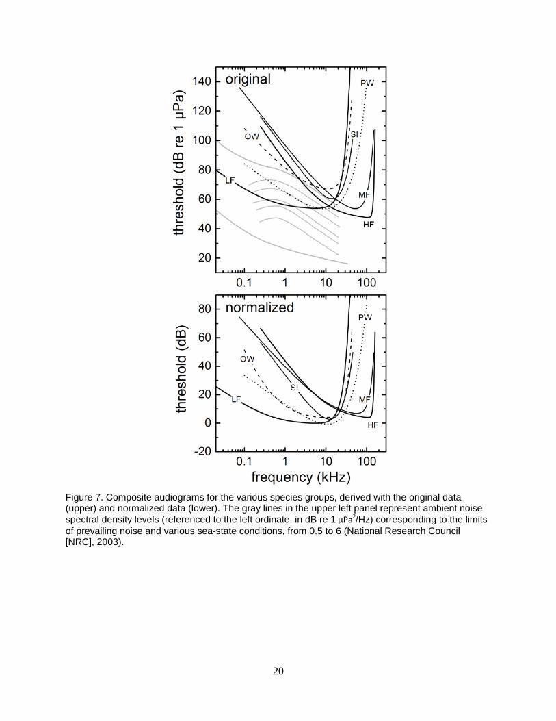
Figure 7. Composite audiograms for the various species groups, derived with the original data (upper) and normalized data (lower). The gray lines in the upper left panel represent ambient noise spectral density levels (referenced to the left ordinate, in dB re 1 μPa2/Hz) corresponding to the limits of prevailing noise and various sea-state conditions, from 0.5 to 6 (National Research Council [NRC], 2003).

21

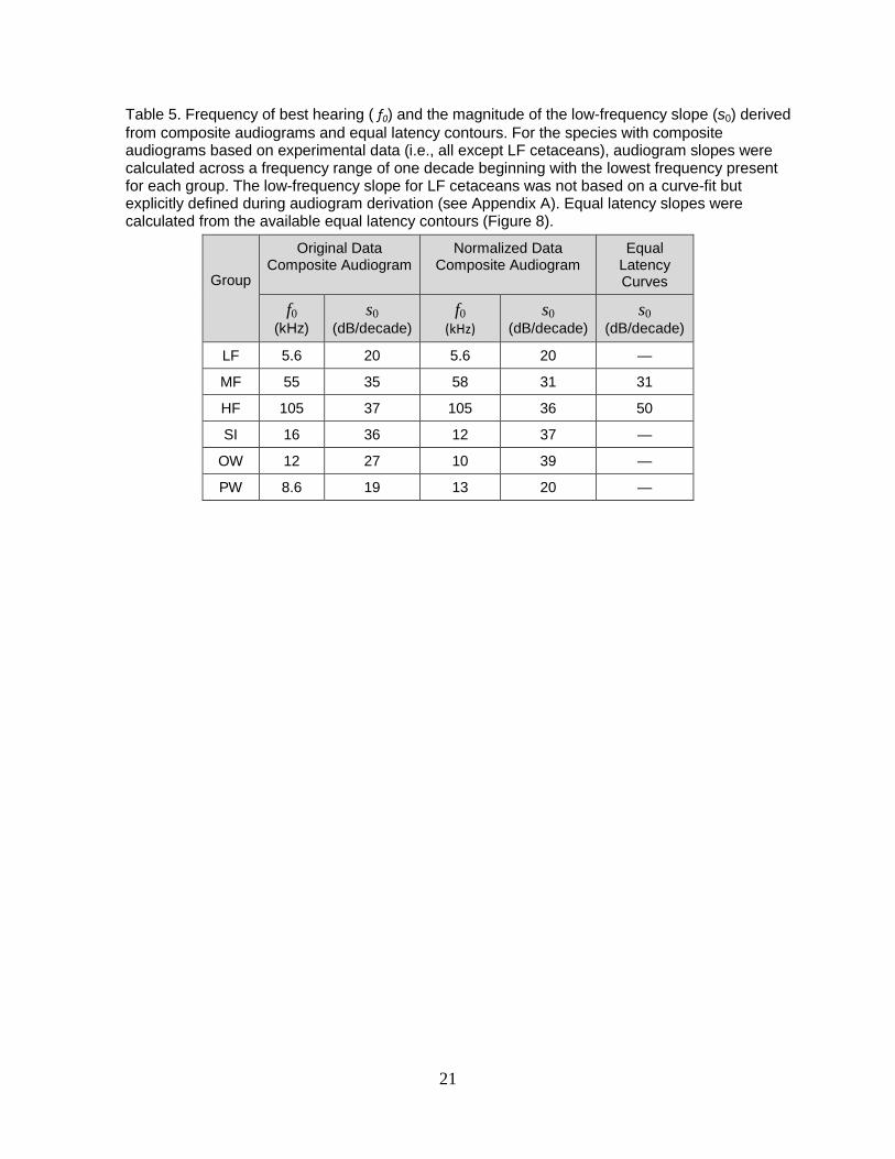
Table 5. Frequency of best hearing ( f0) and the magnitude of the low-frequency slope (s0) derived from composite audiograms and equal latency contours. For the species with composite audiograms based on experimental data (i.e., all except LF cetaceans), audiogram slopes were calculated across a frequency range of one decade beginning with the lowest frequency present for each group. The low-frequency slope for LF cetaceans was not based on a curve-fit but explicitly defined during audiogram derivation (see Appendix A). Equal latency slopes were calculated from the available equal latency contours (Figure 8).

Group

Original Data Composite Audiogram

Normalized Data Composite Audiogram

Equal Latency Curves

f0 (kHz)

s0 (dB/decade)

f0 (kHz)

s0 (dB/decade)

s0 (dB/decade)

LF 5.6 20 5.6 20 —

MF 55 35 58 31 31

HF 105 37 105 36 50

SI 16 36 12 37 —

OW 12 27 10 39 —

PW 8.6 19 13 20 —

22

6. EQUAL LOUDNESS DATA

Finneran and Schlundt (2011) conducted a subjective loudness comparison task with a bottlenose dolphin and used the resulting data to derive equal loudness contours and auditory weighting functions. The weighting functions agreed closely with dolphin TTS data over the frequency range 3 to 56 kHz (Finneran and Schlundt, 2013); however, the loudness data only exist for frequencies between 2.5 and 113 kHz and cannot be used to estimate the shapes of loudness contours and weighting functions at lower frequencies.

23

7. EQUAL LATENCY DATA

Reaction times to acoustic tones have been measured in several marine mammal species and used to derive equal latency contours and weighting functions (Figure 8, Wensveen, Huijser, Hoek, and Kastelein, 2014; Mulsow, Schlundt, Brandt and Finneran, 2015). Unlike the dolphin equal loudness data, the latency data extend to frequencies below 1 kHz and may be used to estimate the slopes of auditory weighting functions at lower frequencies.

Figure 8. Underwater marine mammal equal latency contours are available for Phocoena phocoena (Wensveen et al., 2014) and Tursiops truncatus (Mulsow et al., 2015). The slopes for the contours at low frequencies were obtained from the literature (Phocoena phocoena) or calculated from the best linear-log fits to the lower frequency data. The slope of the contour passing through an SPL approximately 40 dB above the threshold at f0 was selected as the most appropriate based on: (1) human A-weighting, (2) observations that the relationship between equal latency and loudness can break down at higher sensation levels, and (3) for many data sets the slopes increase at higher SPLs rather than decrease as expected. The resulting slopes are listed in Table 5.

24

8. TTS DATA

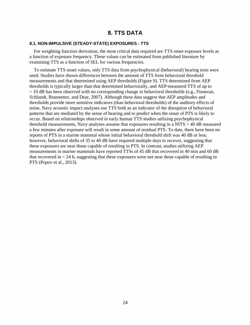
8.1. NON-IMPULSIVE (STEADY-STATE) EXPOSURES - TTS

For weighting function derivation, the most critical data required are TTS onset exposure levels as a function of exposure frequency. These values can be estimated from published literature by examining TTS as a function of SEL for various frequencies.

To estimate TTS onset values, only TTS data from psychophysical (behavioral) hearing tests were used. Studies have shown differences between the amount of TTS from behavioral threshold measurements and that determined using AEP thresholds (Figure 9). TTS determined from AEP thresholds is typically larger than that determined behaviorally, and AEP-measured TTS of up to ~ 10 dB has been observed with no corresponding change in behavioral thresholds (e.g., Finneran, Schlundt, Branstetter, and Dear, 2007). Although these data suggest that AEP amplitudes and thresholds provide more sensitive indicators (than behavioral thresholds) of the auditory effects of noise, Navy acoustic impact analyses use TTS both as an indicator of the disruption of behavioral patterns that are mediated by the sense of hearing and to predict when the onset of PTS is likely to occur. Based on relationships observed in early human TTS studies utilizing psychophysical threshold measurements, Navy analyses assume that exposures resulting in a NITS > 40 dB measured a few minutes after exposure will result in some amount of residual PTS. To date, there have been no reports of PTS in a marine mammal whose initial behavioral threshold shift was 40 dB or less; however, behavioral shifts of 35 to 40 dB have required multiple days to recover, suggesting that these exposures are near those capable of resulting in PTS. In contrast, studies utilizing AEP measurements in marine mammals have reported TTSs of 45 dB that recovered in 40 min and 60 dB that recovered in < 24 h, suggesting that these exposures were not near those capable of resulting in PTS (Popov et al., 2013).

25

Figure 9. TTS measured using behavioral and AEP methods do not necessarily agree, with marine mammal studies reporting larger TTS obtained using AEP methods. For the data above, thresholds were determined using both techniques before and after the same noise exposure. Hearing thresholds were measured at 30 kHz. Behavioral thresholds utilized FM tones with 10% bandwidth. AEP thresholds were based on AM tones with a modulation frequency of 1.05 kHz. Noise exposures consisted of (a) a single, 20-kHz tone with duration of 64 s and SPL of 185 dB re 1 μPa (SEL = 203 dB re 1 μPa2s) and (b) three 16-s tones at 20 kHz, with mean SPL = 193 dB re 1 μPa (cumulative SEL = 210 dB re 1 μPa2s). Data from Finneran et al. (2007).

To determine TTS onset for each subject, the amount of TTS observed after exposures with different SPLs and durations were combined to create a single TTS growth curve as a function of SEL. The use of (cumulative) SEL is a simplifying assumption to accommodate sounds of various SPLs, durations, and duty cycles. This is referred to as an “equal energy” approach, since SEL is related to the energy of the sound and this approach assumes exposures with equal SEL result in equal effects, regardless of the duration or duty cycle of the sound. It is well-known that the equal energy rule will overestimate the effects of intermittent noise, since the quiet periods between noise exposures will allow some recovery of hearing compared to noise that is continuously present with the same total SEL (Ward, 1997). For continuous exposures with the same SEL but different durations, the exposure with the longer duration will also tend to produce more TTS (e.g., Kastak et al., 2007; Mooney et al., 2009; Finneran et al., 2010b). Despite these limitations, however, the equal energy rule is still a useful concept, since it includes the effects of both noise amplitude and duration when predicting auditory effects. SEL is a simple metric, allows the effects of multiple noise sources to be combined in a meaningful way, has physical significance, and is correlated with most TTS growth data reasonably well — in some cases even across relatively large ranges of exposure duration (see Finneran, 2015). The use of cumulative SEL for Navy sources will always over-estimate the effects of intermittent or interrupted sources, and the majority of Navy sources feature durations shorter than the exposure durations typically utilized in marine mammal TTS studies, therefore the use of (cumulative) SEL will tend to over-estimate the effects of many Navy sound sources.

26

Marine mammal studies have shown that the amount of TTS increases with SEL in an accelerating fashion: At low exposure SELs, the amount of TTS is small and the growth curves have shallow slopes. At higher SELs, the growth curves become steeper and approach linear relationships with the noise SEL. Accordingly, TTS growth data were fit with the function

, (10)

where t is the amount of TTS, L is the SEL, and m1 and m2 are fitting parameters. This particular function has an increasing slope when L < m2 and approaches a linear relationship for L > m2 (Maslen, 1981). The linear portion of the curve has a slope of m1/10 and an x-intercept of m2. After fitting Equation (10) to the TTS growth data, interpolation was used to estimate the SEL necessary to induce 6 dB of TTS—defined as the “onset of TTS” for Navy acoustic impact analyses. The value of 6 dB has been historically used to distinguish non-trivial amounts of TTS from fluctuations in threshold measurements that typically occur across test sessions. Extrapolation was not performed when estimating TTS onset; this means only data sets with exposures producing TTS both above and below 6 dB were used.

Figures 10 to 13 show all behavioral and AEP TTS data to which growth curves defined by Equation (10) could be fit. The TTS onset exposure values, growth rates, and references to these data are provided in Table 6. 8.2. NON-IMPULSIVE (STEADY-STATE) EXPOSURES - PTS

Since no studies have been designed to intentionally induce PTS in marine mammals (but see Kastak, Mulsow, Ghoul and Reichmuth, 2008), onset-PTS levels for marine mammals must be estimated. Differences in auditory structures and sound propagation and interaction with tissues prevent direct application of numerical thresholds for PTS in terrestrial mammals to marine mammals; however, the inner ears of marine and terrestrial mammals are analogous and certain relationships are expected to hold for both groups. Experiments with marine mammals have revealed similarities between marine and terrestrial mammals with respect to features such as TTS, age-related hearing loss, ototoxic drug-induced hearing loss, masking, and frequency selectivity (e.g., Nachtigall, Lemonds, and Roitblat, 2000; Finneran et al., 2005). For this reason, relationships between TTS and PTS from marine and terrestrial mammals can be used, along with TTS onset values for marine mammals, to estimate exposures likely to produce PTS in marine mammals (Southall et al., 2007).

A variety of terrestrial and marine mammal data sources (e.g., Ward, Glorig, and Skylar, 1958; Ward, Glorig, and Skylar, 1959; Ward, 1960; Miller, Watson, and Covell, 1963; Kryter, Ward, Miller, and Eldredge, 1966) indicate that threshold shifts up to 40 to 50 dB may be induced without PTS, and that 40 dB is a conservative upper limit for threshold shift to prevent PTS; i.e., for impact analysis, 40 dB of NITS is an upper limit for reversibility and that any additional exposure will result in some PTS. This means that 40 dB of TTS, measured a few minutes after exposure, can be used as a conservative estimate for the onset of PTS. An exposure causing 40 dB of TTS is therefore considered equivalent to PTS onset.

To estimate PTS onset, TTS growth curves based on more than 20 dB of measured TTS were extrapolated to determine the SEL required for a TTS of 40 dB. The SEL difference between TTS onset and PTS onset was then calculated. The requirement that the maximum amount of TTS must be at least 20 dB was made to avoid over-estimating PTS onset by using growth curves based on small amounts of TTS, where the growth rates are shallower than at higher amounts of TTS.

27

8.3. IMPULSIVE EXPOSURES

Marine mammal TTS data from impulsive sources are limited to two studies with measured TTS of 6 dB or more: Finneran et al. (2002) reported behaviorally-measured TTSs of 6 and 7 dB in a beluga exposed to single impulses from a seismic water gun (unweighted SEL = 186 dB re 1 μPa2s, peak SPL = 224 dB re 1 μPa) and Lucke et al. (2009) reported AEP-measured TTS of 7 to 20 dB in a harbor porpoise exposed to single impulses from a seismic air gun (Figure 12(f), TTS onset = unweighted SEL of 162 dB re 1 μPa2s or peak SPL of 195 dB re 1 μPa). The small reported amounts of TTS and/or the limited distribution of exposures prevent these data from being used to estimate PTS onset.

In addition to these data, Kastelein et al. (2015) reported behaviorally-measured mean TTS of 4 dB at 8 kHz and 2 dB at 4 kHz after a harbor porpoise was exposed to a series of impulsive sounds produced by broadcasting underwater recordings of impact pile driving strikes through underwater sound projectors. The exposure contained 2760 individual impulses presented at an interval of 1.3-s (total exposure time was 1 h). The average single-strike, unweighted SEL was approximately 146 dB re 1 μPa2s and the cumulative (unweighted) SEL was approximately 180 dB re 1 μPa2s. The pressure waveforms for the simulated pile strikes exhibited significant “ringing” not present in the original recordings and most of the energy in the broadcasts was between 500 and 800 Hz, near the resonance of the underwater sound projector used to broadcast the signal. As a result, some questions exist regarding whether the fatiguing signals were representative of underwater pressure signatures from impact pile driving.

Several impulsive noise exposure studies have also been conducted without measurable (behavioral) TTS. Finneran et al. (2000) exposed dolphins and belugas to single impulses from an “explosion simulator” (maximum unweighted SEL = 179 dB re 1 μPa2s, peak SPL = 217 dB re 1 μPa) and Finneran et al. (2015) exposed three dolphins to sequences of 10 impulses from a seismic air gun (maximum unweighted cumulative SEL = 193 to 195 dB re 1 μPa2s, peak SPL =196 to 210 dB re 1 μPa) without measurable TTS. Finneran, Dear, Carder, and Ridgway (2003) exposed two sea lions to single impulses from an arc-gap transducer with no measurable TTS (maximum unweighted SEL = 163 dB re 1 μPa2s, peak SPL = 203 dB re 1 μPa). Reichmuth et al. (2016) exposed two spotted seals (Phoca largha) and two ringed seals (Pusa hispida) to single impulses from a 10 in3 sleeve air gun with no measurable TTS (maximum unweighted SEL = 181 dB re 1 μPa2s, peak SPL ~ 203 dB re 1 μPa).

28

Figure 10. TTS growth data for mid-frequency cetaceans obtained using behavioral methods. Growth curves were obtained by fitting Equation (10) to the TTS data as a function of SEL. Onset TTS was defined as the SEL value from the fitted curve at a TTS = 6 dB, for only those datasets that bracketed 6 dB of TTS. Onset PTS was defined as the SEL value from the fitted curve at a TTS = 40 dB, for only those datasets with maximum TTS > 20 dB. Frequency values within the panels indicate the exposure frequencies. Solid lines are fit to the filled symbols; dashed lines are fit to the open symbols. See Table 6 for explanation of the datasets in each panel. Frequencies listed in each panel denote the exposure frequency.

29

Figure 11. TTS growth data for mid-frequency cetaceans obtained using AEP methods. Growth curves were obtained by fitting Equation (10) to the TTS data as a function of SEL. Onset TTS was defined as the SEL value from the fitted curve at a TTS = 6 dB, for only those datasets that bracketed 6 dB of TTS. Onset PTS was defined as the SEL value from the fitted curve at a TTS = 40 dB, for only those datasets with maximum TTS > 20 dB. Frequency values within the panels indicate the exposure frequencies. Solid lines are fit to the filled symbols; dashed lines are fit to the open symbols. See Table 6 for explanation of the datasets in each panel.

30

Figure 12. TTS growth data for high-frequency cetaceans obtained using behavioral and AEP methods. Growth curves were obtained by fitting Equation (10) to the TTS data as a function of SEL. Onset TTS was defined as the SEL value from the fitted curve at a TTS = 6 dB, for only those datasets that bracketed 6 dB of TTS. Onset PTS was defined as the SEL value from the fitted curve at a TTS = 40 dB, for only those datasets with maximum TTS > 20 dB. The exposure frequency is specified in normal font; italics indicate the hearing test frequency. Percentages in panels (b), (d) indicate exposure duty cycle (duty cycle was 100% for all others). Solid lines are fit to the filled symbols; dashed lines are fit to the open symbols. See Table 6 for explanation of the datasets in each panel.

31

Figure 13. TTS growth data for pinnipeds obtained using behavioral methods. Growth curves were obtained by fitting Equation (10) to the TTS data as a function of SEL. Onset TTS was defined as the SEL value from the fitted curve at a TTS = 6 dB, for only those datasets that bracketed 6 dB of TTS. Frequency values within the panels indicate the exposure frequencies. Numeric values in panel (c) indicate subjects 01 and 02. Solid lines are fit to the filled symbols; dashed lines are fit to the open symbols. See Table 6 for explanation of the datasets in each panel.

32

Table 1. Summary of marine mammal TTS growth data and onset exposure levels. Only those data from which growth curves could be generated are included. TTS onset values are expressed in SEL, in dB re 1 μPa2s. Tests featured continuous exposure to steady-state noise and behavioral threshold measurements unless otherwise indicated.

Group Species Subject Frequenc

y (kHz)

Min TTS (dB)

Max

TTS

(dB)

TTS Onse

t (dB

SEL)

TTS growth

rate (dB/dB)

PTS Onset (dB

SEL)

TTS-PTS offset (dB)

Notes Reference Figur

e

MF Tursiops truncatus

BEN 3 0 7 211* 0.21 — —

TTS onset higher than subsequent

test

Finneran, Carder, Schlundt, and Ridgway, 2005a

10(a)

MF Tursiops truncatus NAY 3 0 5 — 0.13 — —

Finneran, Carder, Schlundt and Ridgway, 2005

10(b)

MF Tursiops truncatus BLU 3 4 11 207* 1.5 — — intermittent

Finneran, Carder, Schlundt and Dear, 2010a

10(c)

MF Tursiops truncatus BLU 3 0 23 206* 1.0 240 34

TTS onset higher than subsequent

tests

Finneran, Carder, Schlundt and Dear, 2010b

10(d)

MF Tursiops truncatus TYH 3 0 9 194 0.35 — —

Finneran, Carder, Schlundt and Dear, 2010b

10(e)

MF Tursiops truncatus BLU

3 7.1 10

14.1 20

28.3

0 01000

13 7 13 22 25 30

190 184 179 176 181 177

0.28 0.21 0.48 0.95 1.2 4.5

— ——

213 212 190

— ——37 31 13

Finneran and Schlundt, 2013

10(f) 10(f) 10(g) 10(g) 10(h) 10(h)

MF Tursiops truncatus TYH 40

56.6 00

11 12

182 181

0.46 1.1

——

——

Finneran and Schlundt, 2013

10(i) 10(i)

33

MF Delphinapterus

leucas N/a 32 20 40 — 1.4 195 — AEP Popov et al., 2011b 11(a)

* SELs not used in subsequent analyses to optimize S ELs not us ed in s ubs equent a na lys es to optimize ><Yea r>2011</Yea r><R ecNum>27310</R ecNum><Dis pla yText>(P opov e t a l., 2011b)</DisplayText><record><rec-number>27310</rec-number><foreign-keys><key app="EN" db-id="va09f9fw6rp5s0e905wp9x28vvd0z5zd2sd2" timestficantly larger than 4 min, (iv) data were obtained from AEP testing, or (v) a lower TTS onset was found at a different hearing test frequency (also see Notes).

** Distribution of data did not support an accurate estimate for growth rate (the standard error was four orders of magnitude larger than the slope estimate)

Table 6. Summary of marine mammal TTS growth data and onset exposure levels. (continued)

Group Species Subject Frequency (kHz)

Min TTS (dB)

Max TTS (dB)

TTS Onset

(dB SEL)

TTS growth

rate (dB/dB)

PTS Onset

(dB SEL)

TTS-PTS

Offset (dB)

Notes Reference Figure

MF Delphinapterus

leucas Female

11.2 22.5 45 90

25 38 9

21

50 63 51 31

————

2.8 2.5 3.0 0.8

190 183 193 208

————

AEP Popov et al., 2013

11(b) 11(b) 11(c) 11(c)

MF Delphinapterus

leucas Male

11.2 22.5 45 90

15 28 13 8

48 55 42 24

————

2.5 1.7 2.7 1.5

195 188 198 210

————

AEP Popov et al., 2013

11(d) 11(d) 11(e) 11(e)

MF Delphinapterus

leucas Female 22.5 0 40 184* 1.7 206 22 AEP Popov et al., 2014 11(f)

MF Delphinapterus

leucas Male 22.5 12 40 — 1.2 197 — AEP Popov et al., 2014 11(f)

HF Phocoena phocoena 02 4 2 15 165 0.3 — —

Kastelein, Gransier, Hoek, and Olthuis, 2012

12(a)

HF Phocoena phocoena 02 ~1.5

~1.5 00

32 7

191 197*

2.8 0.4

207 —

16 —

100% duty cycle

10% duty cycle

Kastelein, Schop, Gransier and Hoek, 2014

12(b) 12(b)

HF Phocoena phocoena 02 6.5

6.5 10

13 22

161 176*

0.3 1.3

— 204

— 28

6.5 kHz test

Frequency 9.2 kHz

test Frequency

Kastelein, Schop, Gransier and Hoek, 2014

12(c) 12(c)

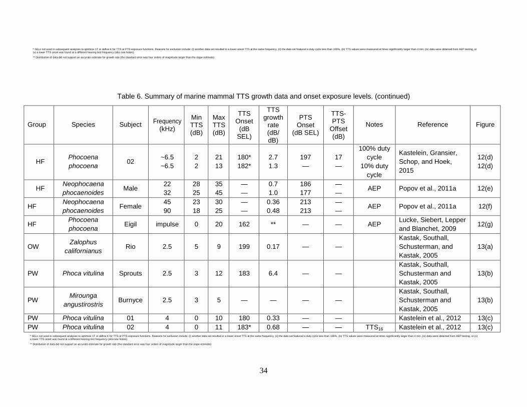
34

* SELs not used in subsequent analyses to optimize ∆T or define K for TTS or PTS exposure functions. Reasons for exclusion include: (i) another data set resulted in a lower onset TTS at the same frequency, (ii) the data set featured a duty cycle less than 100%, (iii) TTS values were measured at times significantly larger than 4 min, (iv) data were obtained from AEP testing, or(v) a lower TTS onset was found at a different hearing test frequency (also see Notes).

** Distribution of data did not support an accurate estimate for growth rate (the standard error was four orders of magnitude larger than the slope estimate)

Table 6. Summary of marine mammal TTS growth data and onset exposure levels. (continued)

Group Species Subject Frequency (kHz)

Min TTS (dB)

Max TTS (dB)

TTS Onset

(dB SEL)

TTS growth

rate (dB/ dB)

PTS Onset

(dB SEL)

TTS-PTS

Offset (dB)

Notes Reference Figure

HF Phocoena phocoena 02 ~6.5

~6.5 22

21 13

180* 182*

2.7 1.3

197 —

17 —

100% duty cycle

10% duty cycle

Kastelein, Gransier, Schop, and Hoek, 2015

12(d) 12(d)

HF Neophocaena phocaenoides Male 22

32 28 25

35 45

——

0.7 1.0

186 177

—— AEP Popov et al., 2011a 12(e)

HF Neophocaena phocaenoides Female 45

90 23 18

30 25

——

0.36 0.48

213 213

—— AEP Popov et al., 2011a 12(f)

HF Phocoena phocoena Eigil impulse 0 20 162 ** — — AEP Lucke, Siebert, Lepper

and Blanchet, 2009 12(g)

OW Zalophus

californianus Rio 2.5 5 9 199 0.17 — — Kastak, Southall, Schusterman, and Kastak, 2005

13(a)

PW Phoca vitulina Sprouts 2.5 3 12 183 6.4 — — Kastak, Southall, Schusterman and Kastak, 2005

13(b)

PW Mirounga

angustirostris Burnyce 2.5 3 5 — — — —

Kastak, Southall, Schusterman and Kastak, 2005

13(b)

PW Phoca vitulina 01 4 0 10 180 0.33 — — Kastelein et al., 2012 13(c) PW Phoca vitulina 02 4 0 11 183* 0.68 — — TTS16 Kastelein et al., 2012 13(c)

* SELs not used in subsequent analyses to optimize ∆T or define K for TTS or PTS exposure functions. Reasons for exclusion include: (i) another data set resulted in a lower onset TTS at the same frequency, (ii) the data set featured a duty cycle less than 100%, (iii) TTS values were measured at times significantly larger than 4 min, (iv) data were obtained from AEP testing, or (v)a lower TTS onset was found at a different hearing test frequency (also see Notes).

** Distribution of data did not support an accurate estimate for growth rate (the standard error was four orders of magnitude larger than the slope estimate)

35

9. TTS EXPOSURE FUNCTIONS FOR SONARS

Derivation of the weighting function parameters utilized the exposure function form described by Equation (2), so that the shapes of the functions could be directly compared to the TTS onset data (Table 6) when available. The function shapes were first determined via the parameters a, b, f1, and f2, then the gain constant K was determined for each group to provide the best fit to the TTS data or estimated TTS onset value at a particular frequency. 9.1. LOW- AND HIGH-FREQUENCY EXPONENTS (A, B)

The high-frequency exponent, b, was fixed at b = 2. This was done to match the previous value used in the Phase 2 functions, since no new TTS data are available at the higher frequencies and the equal latency data are highly variable at the higher frequencies.

The low-frequency exponent, a, was defined as a = s0/20, where s0 is the lower of the slope of the audiogram or equal latency curves (in dB/decade) at low frequencies (Table 5). This causes the weighting function slope to match the shallower slope of the audiogram or equal latency contours at low frequencies. In practice, the audiogram slopes were lower than the equal latency slopes for all groups except the mid-frequency cetaceans (group MF). 9.2. FREQUENCY CUTOFFS (F1, F2)

The frequency cutoffs f1 and f2 were defined as the frequencies below and above the frequency of best hearing (f0, Table 5) where the composite audiogram thresholds values were ∆T-dB above the threshold at f0 (Figure 14). If ∆T = 0, the weighting function shape would match the shape of the inverse audiogram. Values of ∆T > 0 progressively “compress” the weighting function, compared to the audiogram, near the frequency region of best sensitivity. This compression process is included to match the marine mammal TTS data, which show less change in TTS onset with frequency than would be predicted by the audiogram in the region near best sensitivity.

To determine ∆T, the exposure function amplitude defined by Equation (2) was calculated for the mid- and high-frequency cetaceans using ∆T values that varied from 0 to 20 dB. For each ∆T value, the constant K was adjusted to minimize the mean-squared error between the function amplitude and the TTS data (Figre 15). This process was performed using composite audiograms based on both the original and normalized threshold data. Fits were performed using only TTS data resulting from continuous exposures (100% duty cycle). If hearing was tested at multiple frequencies after exposure, the lowest TTS onset value was used.

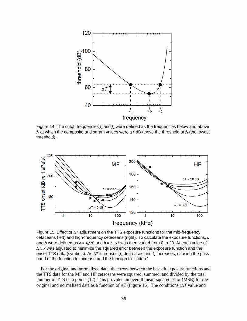
36

Figure 14. The cutoff frequencies f1 and f2 were defined as the frequencies below and above f0 at which the composite audiogram values were ∆T-dB above the threshold at f0 (the lowest threshold).

Figure 15. Effect of ∆T adjustment on the TTS exposure functions for the mid-frequency cetaceans (left) and high-frequency cetaceans (right). To calculate the exposure functions, a and b were defined as a = s0/20 and b = 2. ∆T was then varied from 0 to 20. At each value of ∆T, K was adjusted to minimize the squared error between the exposure function and the onset TTS data (symbols). As ∆T increases, f1 decreases and f2 increases, causing the pass-band of the function to increase and the function to “flatten.”

For the original and normalized data, the errors between the best-fit exposure functions and the TTS data for the MF and HF cetaceans were squared, summed, and divided by the total number of TTS data points (12). This provided an overall mean-squared error (MSE) for the original and normalized data as a function of ∆T (Figure 16). The conditions (∆T value and

37

original/normalized threshold audiograms) resulting in the lowest MSE indicated the best fit of the exposure functions to the TTS data. For the MF and HF cetacean data, the lowest MSE occurred with the normalized threshold data with ∆T = 9 dB. Therefore, f1 and f2 for the remaining species groups were defined using composite audiograms based on normalized thresholds with ∆T = 9 dB.

Figure 16. Relationship between ∆T and the resulting mean-squared error (MSE) between the exposure functions and onset TTS data. The MSE was calculated by adding the squared errors between the exposure functions and TTS data for the MF and HF cetacean groups, then dividing by the total number of TTS data points. This process was performed using the composite audiograms based on original and normalized threshold data and ∆T values from 0 to 20. The lowest MSE value was obtained using the audiograms based on normalized thresholds with ∆T = 9 dB (arrow).

9.3. GAIN PARAMETERS K AND C

The gain parameter K was defined to minimize the squared error between the exposure function and the TTS data for each species group. Note that K is not necessarily equal to the minimum value of the exposure function.

For the low-frequency cetaceans and sirenians, for which no TTS data exist, TTS onset at the frequency of best hearing (f0) was estimated by assuming that, at the frequency of best hearing, the numeric difference between the auditory threshold (in dB SPL) and the onset of TTS (in dB SEL) would be similar to that observed in the other species groups. Table 7 summarizes the onset TTS and composite threshold data for the MF, HF, OW, and PW groups. For these groups, the median difference between the TTS onset and composite audiogram threshold at f0 was 126 dB. In the absence of data, the hearing threshold at f0 for the LF group was set equal to the median threshold at f0 for the other groups (MF, HF, SI, OW, PW, median = 54 dB re 1 μPa). The TTS onset value at f0 is therefore 180 dB re 1 μPa2s for the low-frequency cetaceans (Table 7). For the sirenians, the lowest threshold was 61 dB re 1 μPa, making the onset TTS estimate 187 dB re 1 μPa2s (Table 7).

38

Table 7. Differences between composite threshold values (Figure 5) and TTS onset values at the frequency of best hearing (f0) for the in-water marine mammal species groups. The values for the low-frequency cetaceans and sirenians were estimated using the median difference (126) from the MF, HF, OW, and PW groups.

Group f0 (kHz)

Threshold at f0

(dB re 1 μPa)

TTS onset at f0

(dB re 1 μPa2s) Difference Estimated

Difference

Estimated TTS onset at

f0 (dB re 1 μPa2s)

LF 5.6 54 126 180

MF 55 54 179 125

HF 105 48 156 108

SI 16 61 126 187

OW 12 67 199 132

PW 8.6 53 181 128

Once K was determined, the weighted threshold for onset TTS was determined from the minimum value of the exposure function. Finally, the constant C was determined by substituting parameters a, b, f1, and f2 into Equation (1), then adjusting C so the maximum amplitude of the weighting function was 0 dB; this is equivalent to the difference between the weighted TTS threshold and K [see Equations (3)–(8)].

Table 8 summarizes the various function parameters, the weighted TTS thresholds, and the goodness of fit values between the TTS exposure functions and the onset TTS data. The various TTS exposure functions are presented in Figures 17–20.

Table 8. Weighting function and TTS exposure function parameters for use in Equations (1) and (2) for steady-state exposures. R2 values represent goodness of fit between exposure function and TTS onset data (Table 6).

Group a b f1

(kHz) f2

(kHz) K

(dB) C

(dB)

Weighted TTS

threshold (dB SEL)

R2

LF 1 2 0.20 19 179 0.13 179 —

MF 1.6 2 8.8 110 177 1.20 178 0.825

HF 1.8 2 12 140 152 1.36 153 0.864

SI 1.8 2 4.3 25 183 2.62 186 —

OW 2 2 0.94 25 198 0.64 199 —

PW 1 2 1.9 30 180 0.75 181 0.557

39

Figure 17. Exposure functions (solid lines) generated from Equation (2) with the parameters specified in Table 7. Dashed lines — (normalized) composite audiograms used for definition of parameters a, f1, and f2. A constant value was added to each audiogram to equate the minimum audiogram value with the exposure function minimum. Short dashed line — Navy Phase 2 exposure functions for TTS onset for each group. Filled symbols — onset TTS exposure data (in dB SEL) used to define exposure function shape and vertical position. Open symbols — estimated TTS onset for species for which no TTS data exist.

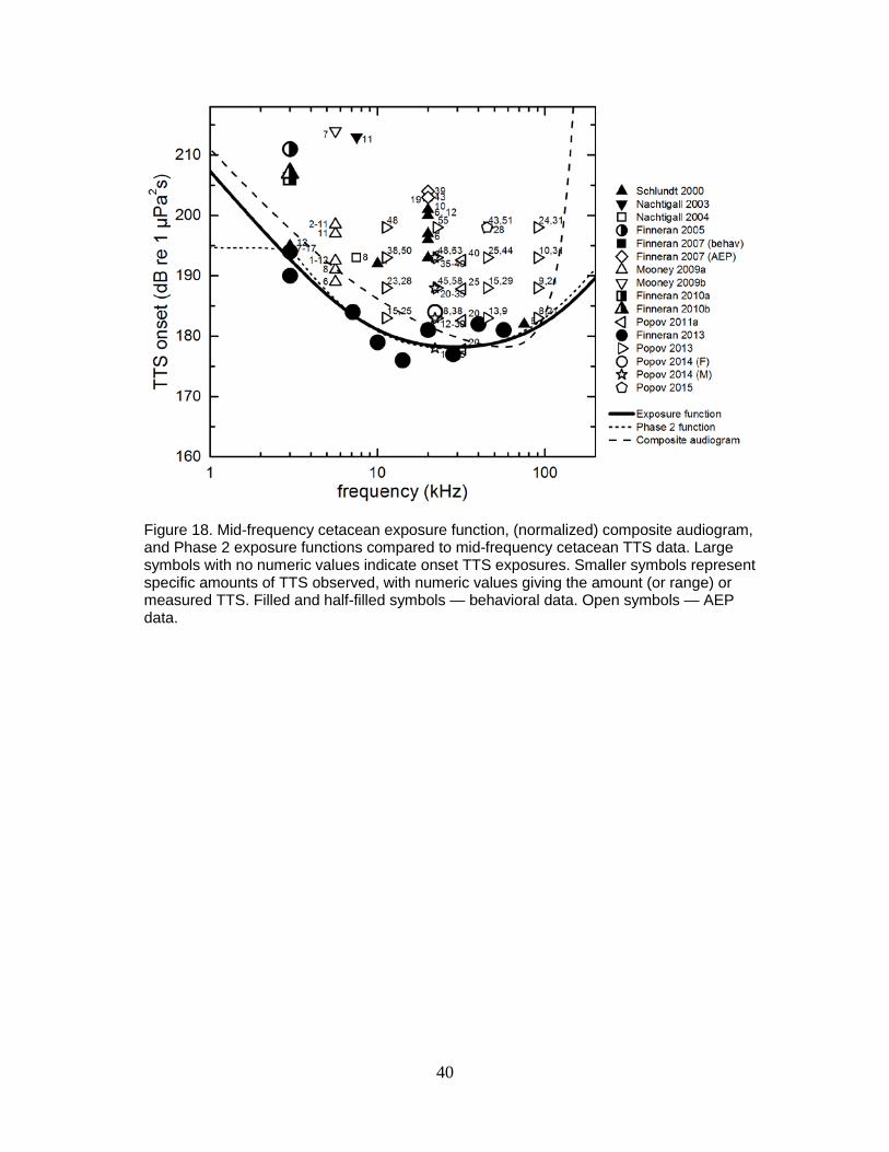
40

Figure 18. Mid-frequency cetacean exposure function, (normalized) composite audiogram, and Phase 2 exposure functions compared to mid-frequency cetacean TTS data. Large symbols with no numeric values indicate onset TTS exposures. Smaller symbols represent specific amounts of TTS observed, with numeric values giving the amount (or range) or measured TTS. Filled and half-filled symbols — behavioral data. Open symbols — AEP data.

41

Figure 19. High-frequency cetacean TTS exposure function, (normalized) composite audiogram, and Phase 2 exposure functions compared to high-frequency cetacean TTS data. Large symbols with no numeric values indicate onset TTS exposures. Smaller symbols represent specific amounts of TTS observed, with numeric values giving the amount (or range) or measured TTS. Filled and half-filled symbols — behavioral data. Open symbols — AEP data.

42

Figure 20. Phocid (underwater) exposure function, (normalized) composite audiogram, and Phase 2 exposure functions compared to phocid TTS data. Large symbols with no numeric values indicate onset TTS exposures. Smaller symbols represent specific amounts of TTS observed, with numeric values giving the amount (or range) or measured TTS.

43

10. PTS EXPOSURE FUNCTIONS FOR SONARS

As in previous acoustic effects analyses (Southall et al., 2007; Finneran and Jenkins, 2012), the shape of the PTS exposure function for each species group is assumed to be identical to the TTS exposure function for that group. Thus, definition of the PTS function only requires the value for the constant K to be determined. This equates to identifying the increase in noise exposure between the onset of TTS and the onset of PTS.

For Phase 2, Navy used a 20-dB difference between TTS onset and PTS onset for cetaceans and a 14-dB difference for phocids, otariids, odobenids, mustelids, ursids, and sirenians (Finneran and Jenkins, 2012). The 20-dB value was based on human data (Ward, Glorig, and Skylar, 1958) and the available marine mammal data, essentially following the extrapolation process proposed by Southall et al. (2007). The 14-dB value was based on a 2.5 dB/dB growth rate reported by Kastak et al. (2007) for a California sea lion tested in air.

For Phase 3, a difference of 20 dB between TTS onset and PTS onset is used for all species groups. This is based on estimates of exposure levels actually required for PTS (i.e., 40 dB of TTS) from the marine mammal TTS growth curves (Table 6), which show differences of 13 to 37 dB (mean = 24, median = 22, n = 9) between TTS onset and PTS onset in marine mammals. These data show most differences between TTS onset and PTS onset are larger than 20 dB and all but one value are larger than 14 dB.

The value of K for each PTS exposure function and the weighted PTS threshold are therefore determined by adding 20 dB to the K-value for the TTS exposure function or the TTS weighted threshold, respectively (see Table 10).

44

11. TTS/PTS EXPOSURE FUNCTIONS FOR EXPLOSIVES

The shapes of the TTS and PTS exposure functions for explosives and other impulsive sources are identical to those used for sonars and other active acoustic sources (i.e., steady-state or non-impulsive noise sources). Thus, defining the TTS and PTS functions only requires the values for the constant K to be determined.

Phase 3 analyses for TTS and PTS from underwater detonations and other impulsive sources follow the approach proposed by Southall et al. (2007) and used in Phase 2 analyses (Finneran and Jenkins, 2012), where a weighted SEL threshold is used in conjunction with an unweighted peak SPL threshold. The threshold producing the greater range for effect is used for estimating the effects of the noise exposure.

Peak SPL and SEL thresholds for TTS were based on TTS data from impulsive sound exposures that produced 6 dB or more TTS for the mid- and high-frequency cetaceans (the only groups for which data are available). The peak SPL thresholds were taken directly from the literature: 224 and 196 dB re 1 μPa, for the mid- and high-frequency cetaceans, respectively (Table 9). The SEL-based thresholds were determined by applying the Phase 3 weighting functions for the appropriate species groups to the exposure waveforms that produced TTS, then calculating the resulting weighted SELs. When this method is applied to the exposure data from Finneran et al. (2002) and Lucke et al. (2009), the SEL-based weighted TTS thresholds are 170 and 140 dB re 1 μPa2s for the mid- and high-frequency cetaceans, respectively (Table 9). Note that the data from Lucke et al. (2009) are based on AEP measurements and may thus under-estimate TTS onset; however, they are used here because of the very limited nature of the impulse TTS data for marine mammals and the likelihood that the high-frequency cetaceans are more susceptible than the mid-frequency cetaceans (i.e., use of the mid-frequency cetacean value is not appropriate). Based on the limited available data, it is reasonable to assume that the exposures described by Lucke et al. (2009), which produced AEP-measured TTS of up to 20 dB, would have resulted in a behavioral TTS of at least 6 dB.

The harbor porpoise data from Kastelein et al. (2015c) were not used to derive the high-frequency cetacean TTS threshold, since the largest observed TTS was only 4 dB. However, these data provide an opportunity to check the TTS onset proposed for the high-frequency cetacean group. Kastelein et al. (2015c) provide a representative frequency spectrum for a single, simulated pile driving strike at a specific measurement location. When the high-frequency cetacean weighting function is applied to this spectrum and the 1/3-octave SELs combined across frequency, the total weighted SEL for a single strike is found to be 114 dB re 1 μPa2s. For 2760 impulses, the cumulative, weighted SEL would then be 148 dB re 1 μPa2s. The average SEL in the pool was reported to be 9 dB lower than the SEL at the measurement position, thus the average, cumulative weighted SEL would be approximately 139 dB re 1 μPa2s, which compares favorably to the high-frequency cetacean TTS threshold of 140 dB re 1 μPa2s derived from the Lucke et al. (2009) air gun data.

For species groups for which no impulse TTS data exist, the weighted SEL thresholds were estimated using the relationship between the steady-state TTS weighted threshold and the impulse TTS weighted threshold for the groups for which data exist (the mid- and high-frequency cetaceans):

, (11)

45

where G indicates thresholds for a species group for which impulse TTS data are not available, indicates the median threshold for the groups for which data exist, the subscript s indicates a steady-state threshold, and the subscript i indicates an impulse threshold (note that since data are only available for the mid- and high-frequency cetaceans the median and mean are identical). Equation (11) is equivalent to the relationship used by Southall et al. (2007), who expressed the relationship as . For the mid- and high-frequency cetaceans, the steady-state TTS thresholds are 178 and 153 dB re 1 μPa2s, respectively, and the impulse TTS thresholds are 170 and 140 dB re 1 μPa2s, respectively, making = 11 dB. Therefore, for each of the remaining groups the SEL-based impulse TTS threshold is 11 dB below the steady-state TTS threshold (Table 9).

To estimate peak SPL-based thresholds, Southall et al. (2007) used Equation (11) with peak-SPL values for the impulse thresholds and SEL-based values for the steady-state thresholds. For the mid- and high-frequency cetaceans, the steady-state (SEL) TTS thresholds are 178 and 153 dB re 1 μPa2s, respectively, and the peak SPL, impulse TTS thresholds are 224 and 196 dB re 1 μPa, respectively, making = -44 dB. Based on this relationship, the peak SPL-based impulse TTS threshold (in dB re 1 μPa) would be 44 dB above the steady-state TTS threshold (in dB re 1 μPa2s), making the peak SPL thresholds vary from 222 to 243 dB re 1 μPa. Given the limited nature of the underlying data, and the relatively high values for some of these predictions, for Phase 3 analyses impulsive peak SPL thresholds are estimated using a “dynamic range” estimate based on the difference (in dB) between the impulsive noise, peak SPL TTS onset (in dB re 1 μPa) and the hearing threshold at f0 (in dB re 1 μPa) for the groups for which data are available (the mid- and high-frequency cetaceans). For the mid-frequency cetaceans, the hearing threshold at f0 is 54 dB re 1 μPa and the peak SPL TTS threshold is 224 dB re 1 μPa, resulting in a dynamic range of 170 dB. For the high-frequency cetaceans, the hearing threshold at f0 is 48 dB re 1 μPa and the peak SPL-based TTS threshold is 196 dB re 1 μPa, resulting in a dynamic range of 148 dB. The median dynamic range for the mid- and high-frequency cetaceans is therefore 159 dB (since there are only two values, the mean and median are equal). For the remaining species groups, the impulsive peak SPL-based TTS thresholds are estimated by adding 159 dB to the hearing threshold at f0 (Table 9).

Since marine mammal PTS data from impulsive noise exposures do not exist, onset-PTS levels for impulsive exposures were estimated by adding 15 dB to the SEL-based TTS threshold and adding 6 dB to the peak pressure based thresholds. These relationships were derived by Southall et al. (2007) from impulse noise TTS growth rates in chinchillas. The appropriate frequency weighting function for each functional hearing group is applied only when using the SEL-based thresholds to predict PTS.

46

Table 9. TTS and PTS thresholds for explosives and other impulsive sources. SEL thresholds are in dB re 1 μPa2s and peak SPL thresholds are in dB re 1 μPa.

Group Hearing Threshold at f0

TTS threshold

PTS threshold

SPL (dB SPL)

SEL (Weighted) (dB SEL)

Weak SPL (dB SPL)

SEL (Weighted) (dB SEL)

Peak SPL (dB SPL)

LF 54 168 213 183 219

MF 54 170 224 185 230

HF 48 140 196 155 202

SI 61 175 220 190 226

OW 67 188 226 203 232

PW 53 170 212 185 218

47

12. SUMMARY

Figure 21 illustrates the shapes of the various Phase 3 auditory weighting functions. Table 10 summarizes the parameters necessary to calculate the weighting function amplitudes using Equation (1).

Figure 21. Navy Phase 3 weighting functions for marine mammal species groups exposed to underwater sound. Parameters required to generate the functions are provided in Table 10.

48

Table 10. Summary of weighting function parameters and TTS/PTS thresholds. SEL thresholds are in dB re 1 μPa2s and peak SPL thresholds are in dB re 1 μPa.

Non-impulsive Impulse

TTS Threshold

PTS Threshold

TTS Threshold

PTS Threshold

Group a b f1

(kHz) f2

(kHz) C

(dB) SEL

(Weighted) SEL

(Weighted) SEL

(Weighted) peak SPL

(Unweighted) SEL

(Weighted) Peak SPL

(Unweighted)

LF 1 2 0.20 19 0.13 179 199 168 213 183 219

MF 1.6 2 8.8 110 1.20 178 198 170 224 185 230

HF 1.8 2 12 140 1.36 153 173 140 196 155 202

SI 1.8 2 4.3 25 2.62 186 206 175 220 190 226

OW 2 2 0.94 25 0.64 199 219 188 226 203 232

PW 1 2 1.9 30 0.75 181 201 170 212 185 218

49

To properly compare the TTS/PTS criteria and thresholds used by Navy for Phase 2 and Phase 3, both the weighting function shape and weighted threshold values must be taken into account; the weighted thresholds by themselves only indicate the TTS/PTS threshold at the most susceptible frequency (based on the relevant weighting function). Since the exposure functions incorporate both the shape of the weighting function and the weighted threshold value, they provide the best means of comparing the frequency-dependent TTS/PTS thresholds for Phase 2 and 3 (Figs 22 and 23).

The most significant differences between the Phase 2 and Phase 3 functions include the following:

(1) Thresholds at low frequencies are generally higher for Phase 3 compared to Phase 2. This is because the Phase 2 weighting functions utilized the “M-weighting” functions (Southall et al., 2007) at lower frequencies, where no TTS existed at that time. Since derivation of the Phase 2 thresholds, additional data have been collected (e.g., Kastelein et al., 2012a; Kastelein et al., 2013b; Kastelein et al., 2014b) to support the use of exposure functions that continue to increase at frequencies below the region of best sensitivity, similar to the behavior of mammalian audiograms and human auditory weighting functions.

(2) In the frequency region near best hearing sensitivity, the Phase 3 underwater thresholds for otariids and other marine carnivores (group OW) are lower than those used in Phase 2. In Phase 2, the TTS onset for the otariids was taken directly from the published literature (Kastak et al., 2005); for Phase 3, the actual TTS data from Kastak et al. (2005) were fit by a TTS growth curve using identical methods as those used with the other species groups.

(3) Impulsive TTS/PTS thresholds near the region of best hearing sensitivity are lower for Phase 3 compared to Phase 2.

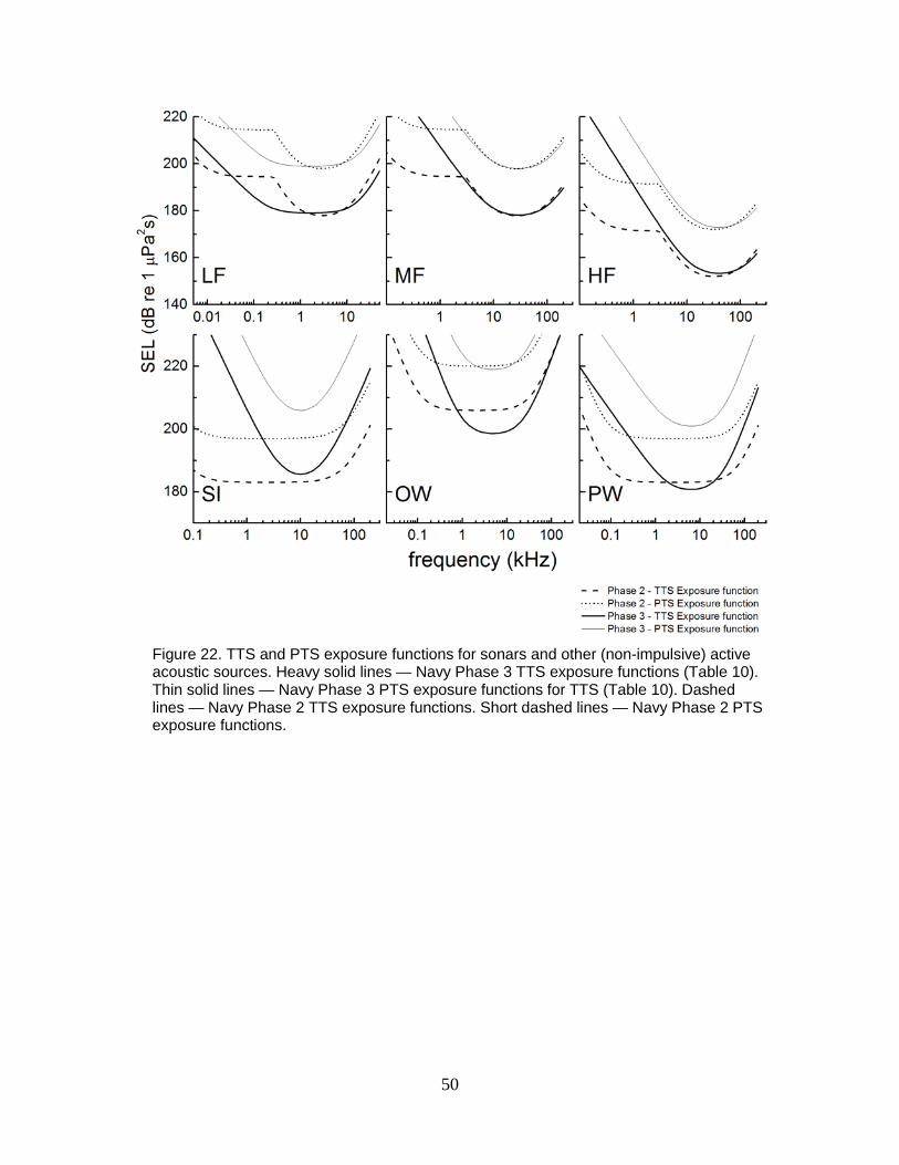
50

Figure 22. TTS and PTS exposure functions for sonars and other (non-impulsive) active acoustic sources. Heavy solid lines — Navy Phase 3 TTS exposure functions (Table 10). Thin solid lines — Navy Phase 3 PTS exposure functions for TTS (Table 10). Dashed lines — Navy Phase 2 TTS exposure functions. Short dashed lines — Navy Phase 2 PTS exposure functions.

51

Figure 23. TTS and PTS exposure functions for explosives, impact pile driving, air guns, and other impulsive sources. Heavy solid lines — Navy Phase 3 TTS exposure functions (Table 10). Thin solid lines — Navy Phase 3 PTS exposure functions for TTS (Table 10). Dashed lines — Navy Phase 2 TTS exposure functions. Short dashed lines — Navy Phase 2 PTS exposure functions.

52

REFERENCES

American National Standards Institute (ANSI). 2001. “Design Response of Weighting Networks for Acoustical Measurements.” ANSI S1.42-2001. Acoustical Society of America.

Awbrey, F. T., J. A. Thomas, and R. A. Kastelein. 1988. “Low-frequency Underwater Hearing Sensitivity In Belugas, Delphinapterus leucas,” Journal of the Acoustical Society of America 84:2273–2275.

Babushina, E. S., G. L. Zaslavsky, and L. l. Yurkevich. 1991. “Air and Underwater Hearing of the Northern Fur Seal - Audiograms and Auditory Frequency Discrimination,” Biofizika 36:904–907.

Brill, R. L., P. W. B. Moore, and L. A. Dankiewicz. 2001. “Assessment of Dolphin (Tursiops truncatus) Auditory Sensitivity and Hearing Loss using Jawphones,” Journal of the Acoustical Society of America 109:1717–1722.

Cranford, T. W., and P. Krysl. 2015. “Fin Whale Sound Reception Mechanisms: Skull Vibration Enables Low-frequency Hearing,” PLoS ONE 10:1–17.

Dow Piniak, W. E., S. A. Eckert, C. A. Harms, and E. M. Stringer. 2012. “Underwater Hearing Sensitivity of the Leatherback Sea Turtle (Dermochelys coriacea): Assessing the Potential Effect of Anthropogenic Noise.” U.S. Department of the Interior, Bureau of Ocean Energy Management Headquarters. Washington, DC.

Finneran, J. J. 2010. “Auditory Weighting Functions and Frequency-dependent Effects of Sound in Bottlenose Dolphins (Tursiops truncatus).” Office of Naval Research (ONR), Washington, DC.

Finneran, J. J. 2015. “Noise-induced Hearing Loss in Marine Mammals: A Review of Temporary Threshold Shift Studies from 1996 to 2015,” Journal of the Acoustical Society of America 138:1702–1726.

Finneran, J. J., D. A. Carder, R. Dear, T. Belting, J. McBain, L. Dalton, and R. H. Ridgway. 2005b. “Pure Tone Audiograms and Possible Aminoglycoside-induced Hearing Loss in Belugas (Delphinapterus leucas),” Journal of the Acoustical Society of America 117:3936–3943.

Finneran, J. J., D. A. Carder, C. E. Schlundt, and R. L. Dear. 2010b. “Growth and Recovery of Temporary Threshold Shift (TTS) at 3 kHz in Bottlenose Dolphins (Tursiops truncatus),” Journal of the Acoustical Society of America 127:3256–3266.

Finneran, J. J., D. A. Carder, C. E. Schlundt, and S. H. Ridgway. 2005a. “Temporary Threshold Shift (TTS) in Bottlenose Dolphins (Tursiops truncatus) Exposed to Mid-Frequency Tones,” Journal of the Acoustical Society of America 118:2696–2705.

53

Finneran, J. J., R. Dear, D. A. Carder, and S. H. Ridgway. “Auditory and Behavioral Responses of California Sea Lions (Zalophus californianus) to Single Underwater Impulses from an Arc-Gap Transducer,” Journal of the Acoustical Society of America 114:1667–1677.

Finneran, J. J., and A. K. Jenkins. 2012. “Criteria and Thresholds for U.S. Navy Acoustic and Explosive Effects Analysis.” Space and Naval Warfare Systems Center Pacific (SSC Pacific), San Diego, CA.

Finneran, J. J., and C. E. Schlundt. 2010. “Frequency-dependent and Longitudinal Changes in Noise-Induced Hearing Loss in a Bottlenose Dolphin (Tursiops truncatus),” Journal of the Acoustical Society of America 128:567–570.

Finneran, J. J. and C. E. Schlundt. 2011. “Subjective Loudness Level Measurements and Equal Loudness Contours in a Bottlenose Dolphin (Tursiops truncatus),” Journal of the Acoustical Society of America 130:3124–3136.

Finneran, J. J., and Schlundt, C.E. 2013. “Effects of Fatiguing Tone Frequency on Temporary Threshold Shift in Bottlenose Dolphins (Tursiops truncatus),” Journal of the Acoustical Society of America 133:1819–1826.

Finneran, J. J., C. E. Schlundt, B. Branstetter, and R. I. Dear. 2007. “Assessing Temporary Threshold Shift in a Bottlenose Dolphin (Tursiops truncatus) Using Multiple Simultaneous Auditory Evoked Potentials,” Journal of the Acoustical Society of America 122:1249–1264.

Finneran, J. J., C. E. Schlundt, B. K. Branstetter, J. Trickey, V. Bowman, and K. Jenkins. 2015. “Effects of Multiple Impulses from a seismic Air Gun on Bottlenose Dolphin Hearing and Behavior,” Journal of the Acoustical Society of America 137:1634–1646.

Finneran, J. J., C. E. Schlundt, D. A. Carder, J. A. Clark, J. A. Young, J. B. Gaspin, and S. H. Ridgway. 2000. “Auditory and Behavioral Responses of Bottlenose Dolphins (Tursiops truncatus) and a Beluga Whale (Delphinapterus Leucas) to Impulsive Sounds Resembling Distant Signatures of Underwater Explosions,” Journal of the Acoustical Society of America 108:417–431.

Finneran, J. J., C. E. Schlundt, R. Dear, D. A. Carder, and S. H. Ridgway. 2002. “Temporary Shift in Masked Hearing Thresholds (MTTS) in Odontocetes after Exposure to Single Underwater Impulses from a Seismic Watergun,” Journal of the Acoustical Society of America 111:2929–2940.

Gaspard, J. C., III, G. B. Bauer, R. L. Reep, K. Dziuk, A. Cardwell, L. Read, and D. A. Mann. 2012. “Audiogram and Auditory Critical Ratios of Two Florida Manatees (Trichechus manatus latirostris),” Journal of Experimental Biology 215:1442–1447.

Gerstein, E. R., L. Gerstein, S. E. Forsythe, J. E. and Blue. 1999. “The Underwater Audiogram of the West Indian Manatee (Trichechus manatus),” Journal of the Acoustical Society of America 105:3575–3583.

54

Ghoul, A., and C. Reichmuth. 2014. “Hearing in the Sea Otter (Enhydra lutris): Auditory Profiles for an Amphibious Marine Carnivore,” Journal of Comparative Physiology A Neuroethology, Sensory, Neural, and Behavioral Physiology 200:967–981.

Heffner, R.S. and Heffner, H.E. 1982. “Hearing in the Elephant (Elephas maximus): Absolute Sensitivity, Frequency Discrimination, and Sound Localization,” Journal of Comparative and Physiological Psychology 96:926–944.

Houser, D. S., D. A. Helweg, and P. W. B. Moore. 2001. “A Bandpass Filter-bank Model of Auditory Sensitivity in the Humpback Whale,” Aquatic Mammals 27:82–91.

Jacobs, D. W. and J. D. Hall. 1972. “Auditory Thresholds of a Fresh Water Dolphin, Inia geoffrensis Blainville,” Journal of the Acoustical Society of America 51:530–533.

Johnson, C. S. 1967. “Sound Detection Thresholds in Marine Mammals,” In Marine Bioacoustics, pp. 247–260. W.N. Tavolga, Ed. Pergamon Press, Oxford, United Kingdom.

Johnson, C. S., McManus, M.W., and Skaar, D. 1989. “Masked Tonal Hearing thresholds in the Beluga Whale,” Journal of the Acoustical Society of America 85:2651–2654.

Kastak, D., Mulsow, J., Ghoul, A., and Reichmuth, C. 2008. “Noise-induced Permanent Threshold Shift in a Harbor Seal,” Journal of the Acoustical Society of America 123:2986(A).

Kastak, D., C. Reichmuth, N. M. Holt, J. Mulsow, B. L. Southall, and R. J. Schusterman, 2007. “Onset, Growth, and Recovery of In-air Temporary Threshold Shift in a California Sea Lion (Zalophus californianus),” Journal of the Acoustical Society of America 122:2916–2924.

Kastak, D., and R. J. Schusterman. 1999. “In-air and Underwater Hearing Sensitivity of a Northern Elephant Seal (Mirounga Angustirostris),” Canadian Journal of Zoology 77:1751–1758.

Kastak, D., B. L. Southall, R. J. Schusterman, and CZ. R. Kastak. 2005. “Underwater Temporary Threshold Shift in Pinnipeds: Effects of Noise Level and Duration,” Journal of the Acoustical Society of America 118:3154–3163.

Kastelein, R. A., P. Bunskoek, M. Hagedoorn, W. W. L. Au, and D. de Haan. 2002a. “Audiogram of a Harbor Porpoise (Phocoena phocoena) Measured with Narrow-band Frequency-modulated Signals,” Journal of the Acoustical Society of America 112:334–344.

Kastelein, R. A., R. Gransier, and L. Hoek. 2013a. “Comparative Temporary Threshold Shifts in a Harbor Porpoise and Harbor Seal, and Severe Shift in a Seal,” Journal of the Acoustical Society of America 134:13–16.

Kastelein, R. A., R. Gransier, L. Hoek, A. Macleod, and J. M. Terhune. 2012b. “Hearing Threshold Shifts and Recovery in Harbor Seals (Phoca vitulina) after Octave-Band Noise Exposure at 4 kHz,” Journal of the Acoustical Society of America 132:2745–2761.

55

Kastelein, R. A., Gransier, R., Hoek, L., and Olthuis, J. 2012a. “Temporary Threshold Shifts and Recovery in a Harbor Porpoise (Phocoena phocoena) after Octave-Band Noise at 4 kHz,” Journal of the Acoustical Society of America 132:3525–3537.

Kastelein, R. A., R. Gransier, L. Hoek, and M. Rambags. 2013b. “Hearing Frequency Thresholds of a Harbor Porpoise (Phocoena phocoena) Temporarily Affected by a Continuous 1.5 kHz Tone,” Journal of the Acoustical Society of America 134:2286–2292.

Kastelein, R. A., R. Gransier, M.A. T. Marijt, and L. Hoek. 2015c. “Hearing Frequency Thresholds of Harbor Porpoises (Phocoena phocoena) Temporarily Affected by Played Back Offshore Pile Driving Sounds,” Journal of the Acoustical Society of America 137:556–564.

Kastelein, R. A., R. Gransier, J. Schop, and L. Hoek. 2015b. “Effects of Exposure to Intermittent and Continuous 6–7 kHz Sonar Sweeps on Harbor Porpoise (Phocoena phocoena) Hearing,” Journal of the Acoustical Society of America 137:1623–1633.

Kastelein, R., R. Gransier, R. van Mierlo, L. Hoek, and C. de Jong. 2011. “Temporary Hearing Threshold Shifts and Recovery in a Harbor Porpoise (Phocoena phocoena) and Harbor Seals (Phoca vitulina) Exposed to White Noise in a 1/1 Octave Band around 4 Khz,” Journal of the Acoustical Society of America 129:2432 (A).

Kastelein, R. A., M. Hagedoorn, W. W. L. Au, and D. de Haan. 2003. “Audiogram of a Striped Dolphin (Stenella coeruleoalba),” Journal of the Acoustical Society of America 113:1130–1137.

Kastelein, R. A., L. Hoek, C. A. F. de Jong, and P. J. Wensveen. 2010. “The Effect of Signal Duration on the Underwater Detection Thresholds of a Harbor Porpoise (Phocoena phocoena) for Single Frequency-Modulated Tonal Signals Between 0.25 and 160 kHz,” Journal of the Acoustical Society of America 128:3211–3222.

Kastelein, R. A., L. Hoek, R. Gransier, M. Rambags, and N. Claeys. 2014b. “Effect of Level, Duration, and Inter-pulse Interval of 1-2 kHz Sonar Signal Exposures on Harbor Porpoise Hearing,” Journal of the Acoustical Society of America 136:412–422.

Kastelein, R. A., J. Schop, R. Gransier, and L. Hoek. 2014a. “Frequency of Greatest Temporary Hearing Threshold Shift in Harbor Porpoises (Phocoena phocoena) Depends on the Noise Level,” Journal of the Acoustical Society of America 136:1410–1418.

Kastelein, R. A., J. Schop, L. Hoek, and J. Covi. 2015a. “Hearing Thresholds of a Harbor Porpoise (Phocoena phocoena) for Narrow-band Sweeps,” Journal of the Acoustical Society of America 138:2508–2512.

Kastelein, R. A., P. Mosterd, B. van Santen, M. Hagedoorn, and D. de Haan. 2002b. “Underwater Audiogram of a Pacific Walrus (Odobenus rosmarus divergens) Measured with Narrow-band Frequency-modulated Signals,” Journal of the Acoustical Society of America 112:2173–2182.

56

Kastelein, R.A., R. van Schie, W. C. Verboom, and D. de Haan. 2005. “Underwater Hearing Sensitivity of a Male and a Female Steller Sea Lion (Eumetopias jubatus),” Journal of the Acoustical Society of America 118:1820–1829.

Kastelein, R. A., P. Wensveen, L. Hoek, and J. M. Terhune. 2009. “Underwater Hearing Sensitivity of Harbor Seals (Phoca Vitulina) for Narrow Noise Bands Between 0.2 and 80 kHz,” Journal of the Acoustical Society of America 126:476–483.

Ketten, D. R. 1994. “Functional Analysis of Whale Ears: Adaptations for Underwater Hearing.” IEEE Proceedings in Underwater Acoustics, vol. 1, pp. 264–270.

Ketten, D. R. 2000. “Cetacean Ears.” In Hearing by Whales and Dolphins, pp. 43–108. W. Au, A. N. Popper, and R. R. Fay, Eds. Springer-Verlag, New York, NY.

Kryter, K. D., W. D. Ward, J. D. Miller, and D. H. Eldredge. 1966. “Hazardous Exposure to Intermittent and Steady-state Noise,” Journal of the Acoustical Society of America 39:451–464.

Lemonds, D. W. 1999. “Auditory Filter Shapes in an Atlantic Bottlenose Dolphin (Tursiops truncatus).” Doctoral thesis. University of Hawaii at Manoa, Honolulu, HI.

Ljungblad, D. K., P.D. Scroggins, and W. G. Gilmartin. 1982. “Auditory Thresholds of a Captive Eastern Pacific Bottle-nosed Dolphin, Tursiops spp.,” Journal of the Acoustical Society of America 72, 1726–1729.

Lucke, K., U. Siebert, P. A. Lepper, and M. A. Blanchet. 2009. “Temporary Shift in Masked Hearing Thresholds in a Harbor Porpoise (Phocoena phocoena) after Exposure to Seismic Airgun Stimuli,” Journal of the Acoustical Society of America 125, 4060–4070.

Martin, K. J., S. C. Alessi, J. C. Gaspard, A. D. Tucker, G. B. Bauer, and D. A. Mann. 2012. “Underwater Hearing in the Loggerhead Turtle (Caretta caretta): A Comparison of Behavioral and Auditory Evoked Potential Audiograms,” Journal of Experiential Biology 215:3001–3009.

Maslen, K. R. 1981. “Towards a Better Understanding of Temporary Threshold Shift of Hearing,” Applied Acoustics 14:281–318.

Miller, J. D., C. S. Watson, and W. P. Covell. 1963. “Deafening Effects of Noise on the Cat,” Acta Oto-Laryngologica Supplement 176:1–88.

Mooney, T. A., P. E. Nachtigall, M. Breese, S. Vlachos, and W. W. L. Au. 2009. “Predicting Temporary Threshold Shifts in a Bottlenose Dolphin (Tursiops truncatus): The Effects of Noise Level and Duration,” Journal of the Acoustical Society of America 125:1816–1826.

Moore, P. W. B., and R. J. Schusterman. 1987. “Audiometric Assessment of Northern Fur Seals, Callorhinus ursinus,” Marine Mammal Science 3:31–53.

Mulsow, J., Houser, D.S., and Finneran, J.J. 2012. “Underwater Psychophysical Audiogram of a Young Male California Sea Lion (Zalophus californianus),” Journal of the Acoustical Society of America 131:4182–4187.

57

Mulsow, J., C. E. Schlundt, L. Brandt, and J. J. Finneran. 2015. “Equal Latency Contours for Bottlenose Dolphins (Tursiops truncatus) and California Sea Lions (Zalophus californianus),” Journal of the Acoustical Society of America 138:2678–2691.

Nachtigall, P. E., W. W. L. Au, , J. Pawloski, and P. W. B. Moore. 1995. “Risso’s Dolphin (Grampus griseus) Hearing Thresholds in Kaneohe Bay, Hawaii.” In Sensory Systems of Aquatic Mammals, pp. 49–53. R.A. Kastelein, J. A. Thomas, and P. E. Nachtigall, Eds. DeSpil Publishers, Woerden, The Netherlands.

Nachtigall, P.E., D. W. Lemonds, and H. L. Roitblat. 2000. “Psychoacoustic Studies of Dolphin and Whale Hearing.” In Hearing by Whales and Dolphins, pp. 330–363. W. W. L. Au, A.N. Popper, and R. R. Fay, Eds. Springer, New York, NY.

National Research Council (NRC). 2003. Ocean Noise and Marine Mammals. National Academies Press. Washington, DC.

Parks, S. E., D. R. Ketten, J. T. O’Malley, and J. Arruda. 2007. “Anatomical Predictions of Hearing in the North Atlantic Right Whale,” The Anatomical Record 290 :734–744.

Pfingst, B. E., R. Hienz, J. Kimm, and J. Miller. 1975. “Reaction-time Procedure for Measurement of Hearing. I. Suprathreshold Functions,” Journal of the Acoustical Society of America 57:421–430.

Popov, V. V., V. O. Klishin, D. I. Nechaev, M. G. Pletenko, V. V. Rozhnov, A. Y. Supin, E. V. Sysueva, E.V., and Tarakanov, M.B. 2011b. “Influence of Acoustic Noises on the White Whale Hearing Thresholds,” Doklady Biological Sciences 440, 332–334.

Popov, V. V., D. I. Nechaev, E. V. Sysueva, V. V. Rozhnov, and A, Y. Supin. 2015. “Spectrum Pattern Resolution after Noise Exposure in a Beluga Whale, Delphinapterus leucas: Evoked Potential Study,” Journal of the Acoustical Society of America 138:377–388.

Popov, V. V., A. Y. Supin, M. G. Pletenko, M. B. Tarakanov, V. O. Klishin, T. N. Bulgakova, and E. I. Rosanova. 2007. “Audiogram Variability in Normal Bottlenose Dolphins (Tursiops truncatus),” Aquatic Mammals 33:24–33.

Popov, V. V., A. Y. Supin, V. V. Rozhnov, D. I. Nechaev, and E. V. Sysueva. 2014. “The Limits of Applicability of the Sound Exposure Level (SEL) Metric to Temporal Threshold Shifts (TTS) in Beluga Whales, Delphinapterus leucas,” Journal of Experiential Biology 217, 1804–1810.

Popov, V. V., A. Y. Supin, V. V. Rozhnov, D. I. Nechaev, E. V. Sysuyeva, V. O. Klishin, M. G. Pletenko, and M. B. Tarakanov. 2013. “Hearing Threshold Shifts and Recovery after Noise Exposure in Beluga Whales Delphinapterus leucas,” Journal of Experiential Biology 216:1587–1596.

Popov, V. V., A. Y Supin, D. Wang, K. Wang, L. Dong, and S. Wang. 2011a. “Noise-induced Temporary Threshold Shift and Recovery in Yangtze Finless Porpoises Neophocaena phocaenoides asiaeorientalis,” Journal of the Acoustical Society of America 130:574–584.

58

Reichmuth, C. 2013. “Equal Loudness Contours and Possible Weighting Functions for Pinnipeds,” Journal of the Acoustical Society of America 134:4210 (A).

Ridgway, S. H., D. A. Carder, T. Kamolnick, R. R. Smith, C. E. Schlundt, and W. R. Elsberry. 2001. “Hearing and Whistling in the Deep Sea: Depth Influences Whistle Spectra But Does Not Attenuate Hearing by White Whales (Delphinapterus leucas) (Odontoceti, Cetacea),” Journal of Experiential Biology 204:3829–3841.

Reichmuth, C., A. Ghoul, A. Rouse, J. Sills, and B. Southall. 2016. “Temporary Threshold Shift not Measured in Spotted or Ringed Seals Exposed to Single Airgun Impulses,” Journal of the Acoustical Society of America (in review).

Reichmuth, C., M. M. Holt, J. Mulsow, J. M. Sills, and B. L. Southall. 2013. “Comparative Assessment of Amphibious Hearing in Pinnipeds,” Journal of Comparative and Physiology A 199:491–507.

Reichmuth, C., and B. L. Southall. 2012. “Underwater Hearing in California sea lions (Zalophus californianus): Expansion and Interpretation of Existing Data,” Marine Mammal Science 28: 358–363.

Sauerland, M., and G. Dehnhardt. 1998. “Underwater Audiogram of a Tucuxi (Sotalia fluviatilis guianensis),” Journal of the Acoustical Society of America 103:1199–1204.

Schlundt, C. E., J. J. Finneran, B. K. Branstetter, R. I Dear, D. S. Houser, and E. Hernandez. 2008. “Evoked Potential and Behavioral Hearing Thresholds in Nine Bottlenose Dolphins (Tursiops truncatus),” Journal of the Acoustical Society of America 123:3506(A).

Sills, J. M., B. L. Southall, and C. Reichmuth. 2014. “Amphibious hearing in spotted seals (Phoca largha): Underwater Audiograms, Aerial Audiograms and Critical Ratio Measurements,” Journal of Experiential Biology 217:726–734.

Sills, J. M., B. L. Southall, and C. Reichmuth. 2015. “Amphibious Hearing in Ringed Seals (Pusa hispida): Underwater Audiograms, Aerial Audiograms and Critical Ratio Measurements,” Journal of Experential Biology 218:2250–2259.

Southall, B. L., A. E. Bowles, W. T. Ellison, J. J. Finneran, R. I. Gentry, C. R. Greene Jr., D. Kastak, D. R. Ketten, J. H. Miller, P. E. Nachtigall, W. J. Richardson, J. A. Thomas, and P. I. Tyack. 2007. “Marine Mammal Noise Exposure Criteria: Initial Scientific Recommendations,” Aquatic Mammals 33:411–521.

Stebbins, W. C. 1966. “Auditory Reaction Time and the Derivation of Equal Loudness Contours for the Monkey,” Journal of the Experimental Analysis of Behavior 9:135–142.

Szymanski, M. D., D. E. Bain, K. Kiehl, S. Pennington, W. Wong, and K. R. Henry. 1999. “Killer Whale (Orcinus orca) Hearing: Auditory Brainstem Response and Behavioral Audiograms,” Journal of the Acoustical Society of America 106:1134–1141.

Terhune, J. M. 1988. “Detection Thresholds of a Harbour Seal to Repeated Underwater High-Frequency, Short-Duration Sinusoidal Pulses,” Canadian Journal of Zoology 66:1578–1582.

59

Thomas, J., N. Chun, W. Au, and K. Pugh. 1988. “Underwater Audiogram of a False Killer Whale (Pseudorca crassidens),” Journal of the Acoustical Society of America 84:936–940.

Tremel, D. P., J. A. Thomas, K. T. Ramierez, G. S. Dye, W. A, Bachman, A. N. Orban, and K. K. Grimm. 1998. “Underwater Hearing Sensitivity of a Pacific White-Sided Dolphin, Lagenorhynchus obliquidens,” Aquatic Mammals 24:63–69.

Tubelli, A. A., A. Zosuls, D. R. Ketten, M. Yamato, and D. C. Mountain. 2012. “A Prediction of the Minke Whale (Balaenoptera acutorostrata) Middle-Ear Transfer Function,” Journal of the Acoustical Society of America 132:3263–3272.

Tyack, P. L, and C. W. Clark. 2000. “Communication and Acoustic Behavior of Dolphins and Whales.” In Hearing by Whales and Dolphins, pp. 156–224. W. W. L. Au, A.N. Popper, and R.R. Fay, Eds. Springer, New York, NY.

Ward, W. D. 1960. “Recovery from High Values of Temporary Threshold Shift,” Journal of the Acoustical Society of America 32:497–500.

Ward, W. D. 1997. “Effects of High-Intensity Sound.” In Encyclopedia of Acoustics, pp. 1497–1507. M. J. Crocker, Ed. Wiley, New York, NY.

Ward, W. D., A. Glorig, and D. L. Sklar. 1958. “Dependence of Temporary Threshold Shift at 4 kc on Intensity and Time,” Journal of the Acoustical Society of America 30:944–954.

Ward, W. D., A. Glorig, and D. L. Sklar. 1959. “Temporary Threshold Shift from Octave-Band Noise: Applications to Damage-Risk Criteria,” Journal of the Acoustical Society of America 31:522–528.

Wartzok, D., and D. Ketten. 1999. “Marine Mammal Sensory Systems.” In The Biology of Marine Mammals. J. E. Reynolds and S. A. Rommel, Eds. Smithsonian Institution Press, Washington, DC.

Wensveen, P. J., L. A. E. Huijser, L. Hoek, and R. A. Kastelein. 2014. “Equal Latency Contours and Auditory Weighting Functions for the Harbour Porpoise (Phocoena phocoena),” Journal Experential Biology 217:359–369.

White, M. J., J. Norris, D. K. Ljungblad, K. Baron, and G. N. di Sciara. 1978. “Auditory Thresholds of Two Beluga Whales (Delphinapterus leucas),” Hubbs Sea World Research Institute, San Diego, CA.

A-1

APPENDIX A

ESTIMATING A LOW-FREQUENCY CETACEAN AUDIOGRAM

A.1 BACKGROUND

Psychophysical and/or electrophysiological auditory threshold data exist for at least one species within each hearing group, except for the low-frequency (LF) cetacean (i.e., mysticete) group, for which no direct measures of auditory threshold have been made. For this reason, an alternative approach was necessary to estimate the composite audiogram for the LF cetacean group.

The published data sources available for use in estimating mysticete hearing thresholds consist of cochlear frequency-place maps created from anatomical measurements of basilar membrane dimensions (e.g., Ketten, 1994; Parks, Ketten, O’Malley, and Arruda, 2007), scaling relationships between inter-aural time differences and upper-frequency limits of hearing (see Ketten, 2000), finite element models of head-related and middle-ear transfer functions (Tubelli et al., 2012; Cranford and Krysl, 2015), a relative hearing sensitivity curve derived by integrating cat and human threshold data with a frequency-place map for the humpback whale (Houser, Helweg, and Moore, 2001), and measurements of the source levels and frequency content of mysticete vocalizations (see review by Tyack and Clark, 2000). All references cited in Appendix A are provided in the References list that begins on page 52 of this report. These available data sources are applied here to estimate a mysticete composite audiogram. Given that these data are limited in several regards and are quite different from the type of data supporting composite audiograms in other species, additional sources of information, such as audiograms from other marine mammals, are also considered and applied to make conservative extrapolations at certain decision points.

Mathematical models based on anatomical data have been used to predict hearing curves for several mysticete species (e.g., Ketten and Mountain, 2009; Cranford and Krysl, 2015). However, these predictions are not directly used to derive the composite audiogram for LF cetaceans for two primary reasons:

1. There are no peer-reviewed publications that provide a complete description of the mathematical process by which frequency-place maps based on anatomical measurements were integrated with models of middle-ear transfer functions and/or other information to derive the predicted audiograms presented in several settings by Ketten/Mountain (e.g., Ketten and Mountain, 2009). As a result, the validity of the resulting predicted audiograms cannot be independently evaluated, and these data cannot be used in the present effort.

2. Exclusion of the Ketten/Mountain predicted audiograms leaves only the Cranford/Krysl predicted fin whale hearing curve (Cranford and Krysl, 2015). However, this curve cannot be used by itself to predict hearing thresholds for all mysticetes because:

a. The Cranford/Krysl model is based on sound transmission through the head to the ear of the fin whale, but does not include the sensory receptors of the

A-2

cochlea. There is therefore no way to properly predict the upper cutoff of hearing and the shape of the audiogram at frequencies above the region of best predicted sensitivity.

b. The audiogram does not possess the typical shape one would expect for an individual with normal hearing based on measurements from other mammals. Specifically, the “hump” in the low-frequency region and the shallow roll-off at high frequencies do not match patterns typically seen in audiometric data from other mammals with normal hearing. Given these considerations, the proposed audiogram cannot be considered representative of all mysticetes without other supporting evidence. Although the specific numeric thresholds from Cranford and Krysl (2015) are not directly used in the revised approach explained here, the predicted thresholds are still used to inform the LF cetacean composite audiogram derivation.

Vocalization data also cannot be used to directly estimate auditory sensitivity and audible

range, since there are many examples of mammals that vocalize below the frequency range where they have best hearing sensitivity, and well below their upper hearing limit. However, it is generally expected that animals have at least some degree of overlap between the auditory sensitivity curve and the predominant frequencies present in conspecific communication signals. Therefore, vocalization data can be used to evaluate, at least at a general level, whether the composite audiogram is reasonable (i.e., to ensure that the predicted thresholds make sense given what we know about animal vocalization frequencies, source levels, and communication range).

The realities of the currently available data leave only a limited amount of anatomical data and finite element modeling results to guide the derivation of the LF cetacean composite audiogram, supplemented with extrapolations from the other marine mammal species groups where necessary and a broad evaluation of the resulting audiogram in the context of whale bioacoustics.

A.2 AUDIOGRAM FUNCTIONAL FORM AND REQUIRED PARAMETERS

Navy Phase 3 composite audiograms are defined by the equation:

, (A1)

where T( f ) is the threshold at frequency f, and T0, F1, F2, A, and B are constants. To understand the physical significance and influence of the parameters T0, F1, F2, A, and B, Equation (A1) may be viewed as the sum of three individual terms:

, (A2)

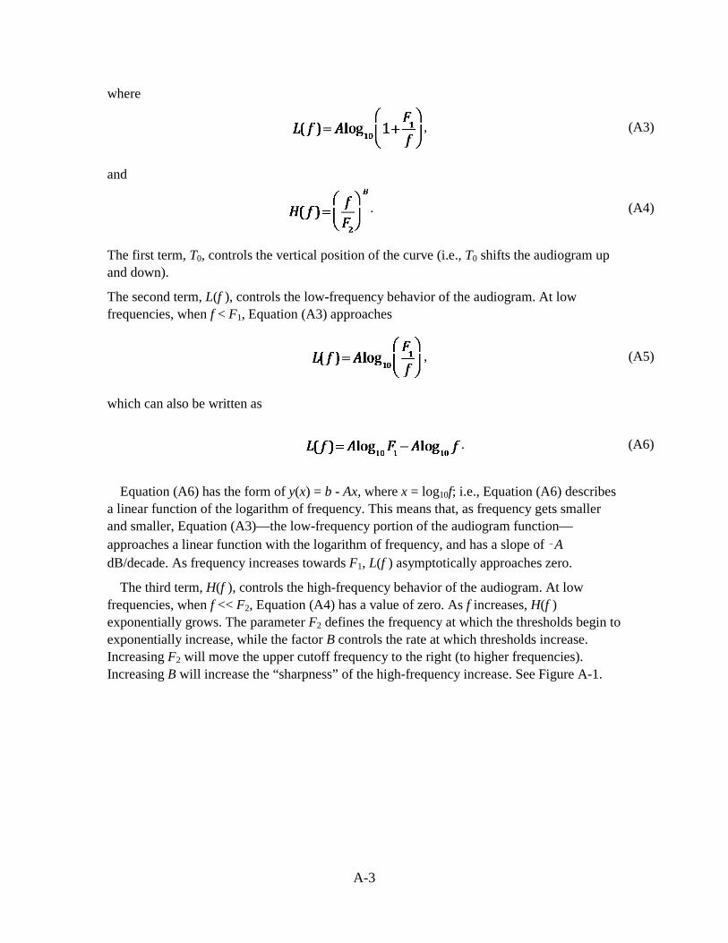
A-3

where

, (A3)

and

. (A4)

The first term, T0, controls the vertical position of the curve (i.e., T0 shifts the audiogram up and down).

The second term, L(f ), controls the low-frequency behavior of the audiogram. At low frequencies, when f < F1, Equation (A3) approaches

, (A5)

which can also be written as

. (A6)

Equation (A6) has the form of y(x) = b - Ax, where x = log10f; i.e., Equation (A6) describes a linear function of the logarithm of frequency. This means that, as frequency gets smaller and smaller, Equation (A3)—the low-frequency portion of the audiogram function—approaches a linear function with the logarithm of frequency, and has a slope of ‑A dB/decade. As frequency increases towards F1, L(f ) asymptotically approaches zero.

The third term, H(f ), controls the high-frequency behavior of the audiogram. At low frequencies, when f << F2, Equation (A4) has a value of zero. As f increases, H(f ) exponentially grows. The parameter F2 defines the frequency at which the thresholds begin to exponentially increase, while the factor B controls the rate at which thresholds increase. Increasing F2 will move the upper cutoff frequency to the right (to higher frequencies). Increasing B will increase the “sharpness” of the high-frequency increase. See Figure A-1.

A-4

Figure A-1. Relationship between estimated threshold, T(f): thick gray line, low-frequency term, L(f): solid line, and high-frequency term, H(f): dashed line.

A.2 ESTIMATING AUDIOGRAM PARAMETERS

To derive a composite mysticete audiogram using Equation (A1), the values of T0, F1, F2, A, and B must be defined. The value for T0 is determined by either adjusting T0 to place the lowest threshold value to zero (to obtain a normalized audiogram), or to place the lowest expected threshold at a specific SPL (in dB re 1 μPa). For Navy Phase 3 analyses, the lowest LF cetacean threshold is defined to match the median threshold of the in-water marine mammal species groups (MF cetaceans, HF cetaceans, sirenians, otariids and other marine carnivores in water, and phocids in water; median = 54 dB re 1 μPa). The choices for the other parameters are informed by the published information regarding mysticete hearing.

The constant A is defined by assuming a value for the low-frequency slope of the audiogram, in dB/decade. Most mammals for which thresholds have been measured have low-frequency slopes ~30 to 40 dB/decade. However, finite element models of middle ear function in fin whales (Cranford and Krysl, 2015) and minke whales (Tubelli et al., 2012) suggest lower slopes, of ~25 or 20 dB/decade, respectively. We therefore conservatively assume that A = 20 dB/decade.

To define F1, we first define the variable T′ as the maximum threshold tolerance within the frequency region of best sensitivity (i.e., within the frequency range of best sensitivity, thresholds are within T′ dB of the lowest threshold). Further, let f ′ be the lower frequency bound of the region of best sensitivity.

A-5

When f = f ′, L(f ) = T′, and Equation (A3) can then be solved for F1 as a function of f ′, T′, and A:

. (A7)

Anatomically based models of mysticete hearing have resulted in various estimates for audible frequency ranges and frequencies of best sensitivity. Houser et al. (2001) estimated best sensitivity in humpback whales to occur in the range of 2 to 6 kHz, with thresholds within 3 dB of best sensitivity from ~1.4 to 7.8 kHz. For right whales, Parks et al. (2007) estimated the audible frequency range to be 10 Hz to 22 kHz. For minke whales, Tubelli et al. (2012) estimated the most sensitive hearing range, defined as the region with thresholds within 40 dB of best sensitivity, to extend from 30 to 100 Hz up to 7.5 to 25 kHz, depending on the specific model used. Cranford and Krysl (2015) predicted best sensitivity in fin whales to occur at 1.2 kHz, with thresholds within 3-dB of best sensitivity from ~1 to 1.5 kHz. Together, these model results broadly suggest best sensitivity (thresholds within ~3 dB of the lowest threshold) from ~1 to 8 kHz, and thresholds within ~40 dB of best sensitivity as low as ~30 Hz and up to ~25 kHz.

Based on this information, we assume LF cetacean thresholds are within 3 dB of the lowest threshold over a frequency range of 1 to 8 kHz, therefore T′ = 3 dB and f ′= 1 kHz, resulting in F1 = 0.41 kHz [Equation (A7)]. In other words, we define F1 so that thresholds are ≤ 3 dB relative to the lowest threshold when the frequency is within the region of best sensitivity (1 to 8 kHz).

To define the high-frequency portion of the audiogram, the values of B and F2 must be estimated. To estimate B for LF cetaceans, we take the median of the B values from the composite audiograms for the other in-water marine mammal species groups (MF cetaceans, HF cetaceans, sirenians, otariids and other marine carnivores in water, and phocids in water). This results in B = 3.2 for the LF cetaceans. Once B is defined, F2 is adjusted to achieve a threshold value at 30 kHz of 40 dB relative to the lowest threshold. This results in F2 = 9.4 kHz. Finally, T0 is adjusted to set the lowest threshold value to 0 dB for the normalized curve, or 54 dB re 1 μPa for the non-normalized curve; this results in T0 = -0.81 and 53.19 for the normalized and non-normalized curves, respectively.

The resulting composite audiogram is shown in Figure A-2. For comparison, predicted audiograms for the fin whale (Cranford and Krysl, 2015), and humpback whale (Houser et al., 2001) are included. The LF cetacean composite audiogram has lowest threshold at 5.6 kHz, but the audiogram is fairly shallow in the region of best sensitivity, and thresholds are within 1 dB of the lowest threshold from ~1.8 to 11 kHz, and within 3 dB of the lowest threshold from ~0.75 to 14 kHz. Low-frequency (< ~500 Hz) thresholds are considerably lower than those predicted by Cranford and Krysl (2015). High-frequency thresholds are also substantially lower than those predicted for the fin whale, with thresholds at 30 kHz only 40 dB above best hearing thresholds, and those at 40 kHz approximately 90 dB above best threshold. The resulting LF composite audiogram appears reasonable in a general sense relative the predominant frequencies present in mysticete conspecific vocal communication

A-6

signals. While some species (e.g., blue whales) produce some extremely low (e.g., 10 Hz) frequency call components, the majority of mysticete social calls occur in the few tens of Hz to few kHz range, overlapping reasonably well with the predicted auditory sensitivity shown in the composite audiogram (within ~0 to 30 dB of predicted best sensitivity). A general pattern of some social calls containing energy shifted below the region of best hearing sensitivity is well-documented in other low-frequency species including many phocid seals (see Wartzok and Ketten, 1999) and some terrestrial mammals, notably the Indian elephant (Heffner and Heffner, 1982).

Figure A-2. Comparison of proposed LF cetacean thresholds to those predicted by anatomical and finite-element models.

Table A-1. Sample table.

Type Change in Rating Level (%)

-4 -3 -2 -1 0 1 2 Fusce 0 0 0 0 50 50 0 T Fuscete ICB 0 0 2 5 30 40 16 Fusceher ICB 2 0 0 2 43 35 6 T F t

0 0 40 0 20 10 30 FusceRAT 0 7 0 10 52 14 10

5f. WORK UNIT NUMBER

REPORT DOCUMENTATION PAGE Form Approved OMB No. 0704-01-0188

The public reporting burden for this collection of information is estimated to average 1 hour per response, including the time for reviewing instructions, searching existing data sources, gathering and maintaining the data needed, and completing and reviewing the collection of information. Send comments regarding this burden estimate or any other aspect of this collection of information, including suggestions for reducing the burden to Department of Defense, Washington Headquarters Services Directorate for Information Operations and Reports (0704-0188), 1215 Jefferson Davis Highway, Suite 1204, Arlington VA 22202-4302. Respondents should be aware that notwithstanding any other provision of law, no person shall be subject to any penalty for failing to comply with a collection of information if it does not display a currently valid OMB control number.

PLEASE DO NOT RETURN YOUR FORM TO THE ABOVE ADDRESS. 1. REPORT DATE (DD-MM-YYYY) 2. REPORT TYPE 3. DATES COVERED (From - To)

4. TITLE AND SUBTITLE 5a. CONTRACT NUMBER

5b. GRANT NUMBER

5c. PROGRAM ELEMENT NUMBER

5d. PROJECT NUMBER

5e. TASK NUMBER

6. AUTHORS

7. PERFORMING ORGANIZATION NAME(S) AND ADDRESS(ES) 8. PERFORMING ORGANIZATION REPORT NUMBER

10. SPONSOR/MONITOR’S ACRONYM(S)

11. SPONSOR/MONITOR’S REPORTNUMBER(S)

9. SPONSORING/MONITORING AGENCY NAME(S) AND ADDRESS(ES)

12. DISTRIBUTION/AVAILABILITY STATEMENT

13. SUPPLEMENTARY NOTES

14. ABSTRACT

15. SUBJECT TERMS

16. SECURITY CLASSIFICATION OF:a. REPORT b. ABSTRACT c. THIS PAGE

17. LIMITATION OFABSTRACT

18. NUMBEROFPAGES

19a. NAME OF RESPONSIBLE PERSON

19B. TELEPHONE NUMBER (Include area code)

Standard Form 298 (Rev. 8/98) Prescribed by ANSI Std. Z39.18

December 2016 Final

Auditory Weighting Functions and TTS/PTS Exposure Functions for Marine Mammals Exposed to Underwater Noise

SSC Pacific 53560 Hull Street San Diego, CA 92152–5001 TR 3026

Approved for public release; distribution is unlimited.

This is the work of the United States Government and therefore is not copyrighted. This work may be copied and disseminated without restriction. Many SSC San Diego public release documents are available in electronic format at http://www.spawar.navy.mil/sti/publications/pubs/index.html

The U.S. Navy’s Tactical Training Theater Assessment and Planning (TAP) Program addresses environmental challenges that affect Navy trainingranges and operating areas. As part of the TAP process, acoustic effects analyses are conducted to estimate the potential effects of Navy activities that introduce high-levels of sound or explosive energy into the marine environment. Acoustic effects analyses begin with mathematical modeling to predict the sound transmission patterns from Navy sources. These data are then coupled with marine species distribution and abundance data to determine the sound levels likely to be received by various marine species. Finally, criteria and thresholds are applied to estimate the specific effects that animals exposed to Navy-generated sound may experience.

This document describes the rationale and steps used to define proposed numeric thresholds for predicting auditory effects on marine mammals exposed to active sonars, other (non-impulsive) active acoustic sources, explosives, pile driving, and air guns for Phase 3 of the TAP Program. Since the derivation of TAP Phase 2 acoustic criteria and thresholds, important new data have been obtained related to the effects of noise on marine mammal hearing. Therefore, for Phase 3, new criteria and thresholds for the onset of temporary and permanent hearing loss have been developed, following a consistent approach for all species of interest and utilizing all relevant, available data. The effects of noise frequency on hearing loss are incorporated by using auditory weighting functions to emphasize noise at frequencies where a species is more sensitive to noise and de-emphasize noise at frequencies where susceptibility is low.

marine mammal hearing; acoustic effects analyses; mathematical modeling; sound transmission patterns from Navy sources; proposed numeric thresholds; noise frequency; auditory weighting functions

J. J. Finneran

U U U UU 79 (619) 767–4098

J. J. Finneran

Commander, U.S. Fleet Forces Command1562 Mitscher AveNorfolk, Va 23551

INITIAL DISTRIBUTION 84500 Library (1) 85300 Archive/Stock (1) 71510 J. J. Finneran (1) Defense Technical Information Center Fort Belvoir, VA 22060–6218 (1)

Approved for public release.

SSC Pacific San Diego, CA 92152-5001