NASA Technical Memorandum 79302

ATIME DEPENDENT DIFFERENCE THEORY

FOR SOUND PROPAGATION

INDUCTS WITH FLOW

(NASA-TM-79302) A TIME DEPENDENT DIFFERENCE N80-12823 THEORY FOR SOUND PROPAGATION IN DUCTS WITH FlOW (NASA) 38 p HC A03/Mr A01 CSCL 20A

Unclas G3/71 46206

K. J. Baumeister

Lewis Research Center

Cleveland, Ohio y - 4

Prepared for the

Ninety-eighth Meeting of the Acoustical Society of America Salt Lake City, Utah, November 26-30, 1979

L

A TIME DEPENDENT DIFFERENCE THEORY

FOR SOUND PROPAGATION IN DUCTS WITH FLOW

K. J. Baumeister

NASA Lewis Research Center Cleveland, Ohio

ABSTRACT.

U% A time dependent numerical solution of the linearized continuity

and momentum equation is developed for sound propagation in a two­

dimensional straight hard or soft wall duct with a sheared mean flow.

The time dependent governing acoustic-difference equations and boundary

conditions are developed along with a numerical determination of the

maximum stable time increments. The analysis begins with a harmonic

noise source radiating into a quiescent duct. This explicit iteration

method then calculates stepwise in real time to obtain the transient

as well as the "steady" state solution of the acoustic field. Example

calculations are presented for sound propagation in hard and soft wall

ducts, with no flow and with plug flow. Although the problem with

sheared flow has been formulated and programmed, sample calculations

have not yet been examined. So far, the time dependent finite dif­

ference analysis has been found to be superior to the steady state

finite difference and finite element techniques because of shorter

solution times and the elimination of large matrix storage require­

ments.

2

List of Symbols

c* ambient speed of sound, m/s0

f frequency, Hz

H duct height, m

I number of axial grid points

J number of transverse grid points

k number of time steps

L length of duct, m

M Mach number M(y), U!/c0

n transverse mode number

P time dependent acoustic pressure, P /p c0 p spatially dependent acoustic pressure

Ps spatially dependent solution of Wave Equation

T period, l/f", sac

4.-A

t dimensionless time, t /T

At time step

U' mean flow velocity U' (Y), m/sec

u axial acoustic velocity, u /c0

4.- 4

v transverse acoustic velocity, v /c"0

x axial coordinate, x /H

&axial grid spacing

y dimensionless transverse coordinate, y IAHI

Ay transverse grid spacing

3

Z

astability

TI

a

P

X

w

c

e

i

j

o

s

t

*

k

(1)

(2)

impedance, kg/m2sec

factor, eq. (29)

specific acoustic impedance

dimensionless frequency, H~f /c0

dimensionless resistance

ambient air density, kg/m 3

dimensionless reactance

angular frequency

Subscripts

calculation, time

exit condition

axial index (Fig. 1)

transverse index (Fig. 1)

ambient condit-ion

spatial value

transient

Superscripts

dimensional quantity

time step index

real part

imaginary part

L

INTRODUCTION

Both finite difference and finite element numerical techniques

(refs. I to 27) have been developed to study sound propagation with

axial variations in Mach number, wall impedance, and duct geometry as

might be encountered in a typical turbojet engine. Generally, the

numerical solutions have been limited to low frequency sound and short

ducts, because many grid points or elements were required to resolve

the axial wavelength of the sound. As shown in reference 1 (eq. (77))

for plane wave propagation, the number of axial grid points or ele­

ments is directly proportional to the sound frequency and duct Vength,

and inversely proportional to the difference of unity minus the Mach

number (ref. 2). This later dependence also severely limits the ap­

plication of numerical techniques for high Mach number inlets.

Customarily, the pressure and acoustic velocities are assumed to

be simple harmonic functions of time; thus," the governing linearized

gas-dynamic equations (ref. 28- pg. 5) become independent of time.

The matrices associated with the numerical solution to the time inde­

pendent equations must be solved exactly using such methods as Gauss

elimination. As a result, large arrays of matrix elements must be

stored which tax the storage capacity of even the largest computer.

In an unpublished work at NASA Lewis Research Center by the author

using reference 29, as well as in the work of Quinn (ref. 23, pg. 3),

the matrix has been modified to allow iteration techniques; unfortu­

nately, the convergence is too slow to be of any practical value.

5

Other approaches, such as in reference 30, might still offer iterative

possibilities.

Some special techniques have been developed to overcome the dif­

ficulties of low frequency, short ducts, and low Mach numbers.. As

shown in references 3 and 10, the wave envelope numerical technique

can reduce the required number of grid points by an order of magnitude.

In reference 20, this technique was used to optimize multi-element

liners of long lengths at high frequencies. At the present time, this

technique has been applied only to the simple cases of no flow and plug

flow. A numerical spatial marching technique was also developed in

references 15 and 18. Compared to the standard finite difference or

finite element boundary value approaches, the numerical marching tech­

nique is orders of magnitude shorter in computational time and required

computer storage. The marching technique is limited to high frequencies

and to cases where reflections are small.

As an alternative to the previously developed steady state theories,

a time dependent numerical solution is developed herein for noise propa­

gation in a two-dimensional soft wall duct with parallel sheared mean

flow. Advantageously, matrix storage requirements are significantly

reduced in the time dependent analysis. The analysis begins with a

noise source radiating into an initially quiescent duct. This explicit

method calculates stepwise in real time to obtain the transient as well

as the "steady" state solution of the acoustic field. The total time

required for the analysis to calculate the "steady" state acoustic field

6

will determine the usefulness of the time dependent technique.

Time dependent numerical techniques have been applied extensively

to one-dimensional sound propagation (ref. 31, pg. 258 andref. 32),

two-dimensional vibration problems (ref. 33, pg.. 452) and the more

general problem of compressible fluid flow (ref. 34). References 35

and 36 discuss in detail the stability of time dependent numerical solu­

.t'ins.

In a companion paper to this work (ref. 37), the explicit time

iteration techniques of references 31 to 36 are extended to include

soft-wail impedance boundary conditions which would be encountered

in inlets and exhaust ducts of turbo-fan jet engines. The analysis

applies to two-dimensional straight hard and soft wall ducts without

flow. In the absence of mean flow, the governing acoustic equation

was the classic second order wave equation. The time dependent solu­

tion to the wave equation was found to be superior to the conventional

steady numerical analysis because of much shorter solution times and

the elimination of large matrix storage requirements.

When parallel shear flow occurs in a duct, the second order formu­

lation of reference 37 cannot' be used' since the governing differential.

wave equation is third order (ref. 28, pg. 9). Rather than attempt to

solve a third order wave equation, in the present paper the first

order equations of continuity and momentum will be solved simultane­

ously. First, the governing acoustic equations and boundary conditions

7

are presented for time dependent propagation in a parallel sheared mean

flow. Next, the governing acoustic-difference equations and boundary

conditions are derived. The two-dimensional stability theory is then

used as a guide to estimate the maximum stable t-ime increment. Immedi­

ately following the mathematical development, numerical solutions are

presented for one-and-two-dimensional hard and soft-wall ducts. The

results are compared with the corresponding steady state analytical

results. Finally, the times required to perform both the time dependent

and steady state analyses are compared for increasing number of grid

points.

I. GOVERNING EQUATIONS AND BOUNDARY CONDITIONS

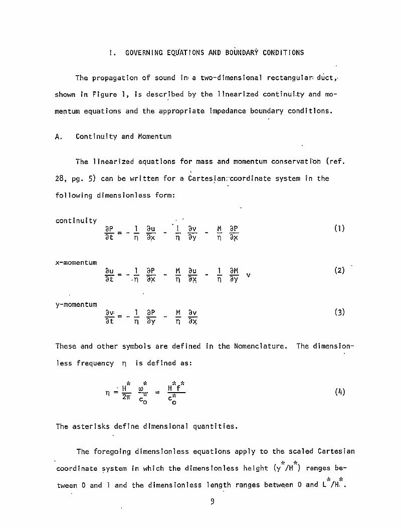
The propagation of sound in,a two-dimensional rectangular duct,,

shown in Figure 1, is described by the linearized continulty and mo­

mentum equations and the appropriate impedance boundary conditions.

A. Continuity and Momentum

The linearized equations for mass and momentum conservatibh (ref.

28, pg. 5) can be written for a Cartesian:coordinate system in the

following dimensionless form:

continuity BP 1 I yv M TuBP (1)0t n1 rxnly na

x-momentum auP -- T W -TM au I TV@M (2)

- Tx ? ByTI n

y-momentum Dv- 1 3P M v (3) at By Ti x

These and other symbols are defined in the Nomenclature. The dimension­

less frequency rl is defined as:

H w Hf (4) co c0

The asterisks define dimensional quantities.

The foregoing dimensionless equations apply to the scaled Cartesian

coordinate system in which the dimensionless height (y /H ) ranges be­

tween 0 and I and the dimensionless length ranges between 0 and L /H..

9

B. Wall Boundary Conditions

The boundary condition on the transverse acoustic velocity v at

the surface of a sound absorbent soft-wall duct canbe expressed in terms

of a specific acoustic impedance

v(x,l,t) = P(x,i,t) (5)

where the complex specific wall impedance is defined as

z - + ix (6)

At the lower wall, the sign on is changed to account for the vector

nature of v.

In addition to equation (5), another form of the wall impedance con­

dition will be considered. Substituting equation (5) into equation (3),

noting that the Mach number is zero at the wall, and assuming is

a constant independent of time, then

DP = -n3P (7)

This form of the impedance boundary condition cannot be used for plug

flow when a soft wall Ls present.

C. Entrance Condition

The boundary condi-tion at the source plane P(o,y,t) can be of any

general form with both transverse variations in pressure and multiple

10

frequency content. However, the numerical technique will be compared later

to previous solut-lons in which the pressure and acoustic velocities were as­

sumed to be plane waves at the entrance and to vary as e or in dimen­

i2Trtsionless form as e Therefore, the source boundary condition used here

is

I27tP(o,y,t) = e (8)

D. Exit Impedance

In a manner similar to the wall impedance, the axial acoustic velocity

at the duct exit can be expressed in terms of a specific acoustic exit-im­

pedance Ce as

**P(L* /H*,y,t)() u(L /H ,y,t) Ce

For the plane wave propagation to be considered herein, Ce is taken to be

equal to unity, which is exact for plane wave propagation in an infinite

hard-wall duct. Also, choosing e to be equal to unity has lead to close

agreement between numerical and analytical results for plane wave propaga­

tion into a soft-wall duct (refs. I and 3). More general values for the

exit impedance can be found in references 7, 15 (eq. B-4), 16, or 18 (fig.

7).

E. Initial Conditions

For times equal to or less than zero, the duct is assumed quiescent;

that is, the acoustic pressure and velocities are taken to be zero. For

11

times greater than zero, the application of the noise,source, equation

(8), will drive the pressures in the duct.

F. Complex Notation

Because of the introduction of complex notation for the noise

source and wall impedance, all the dependent variables are complex.

The superscript (1)will represent the real term while (2)will repre­

sent the imaginary term

p = p(1) + ip(2) (10)

A similar notation applies to- the acoustic velocities.

12

II. DIFFERENCE EQUATIONS

Instead of a continuous solution for pressure in space and time,

the finite difference approximations will determine the pressure at

isolated grid points in space as shown in Figure I and at discrete time

steps At. Starting from the known initial conditions at t=O and the

boundary conditions, the finite difference algorithm will march-out the

solution to later times.

A. Central Region

Away from the duct boundaries of Figure 1, the derivatives in the

governing equations can be represented by the following differences in

time and space:

k+I k (k k l- k (ll)

At = -2Ax s/ 2Ay

kk

ij -- lP -n 2Ax

k+l k k+l k+lI-kk y i-i u i-li) (12)I+LJ- y'u +l~j

At 2Ax 2Ax2A

k V. .a

13

k+l k k+l k+lk - vj',j _! P I l - rj+ - v1+1 - vHi-l ((3)

At T1 2AY T 2Ax

where i and j denote the space indices, k the time index and Ax, Ay, At

are the space and time mesh spacing respectively. All spacings are as­

sumed constant. The time is defined as

k+l k t = t + At = (k+ ])At (14)

Solving equations (11), (12), and (13) for the acoustic pressures and

velocities yields

continuity

k+l k At k k I At k kPi,j 2k+1 kj

Ax It+ Uj - 2%A" i,j+l vi'j- (15)2IATx +I) i.U - '. \ 15

kM At (k27 Zx (Pi+l,j -1-I

x-momentum

k+l k I At kIli }M AtUlij = i~j 2n Ax Pi+],j (16)- Pi-IO 2T Ax U l ,jjui (16)

At aM k

14

y-momentum

k+lv- k At (k+l k+l M~- k - k (17) i'j 2y Pi,jij -P i,j-i) 2q Ax i+l,j Vi-l,j

Equations (15), (16), and (17) are algorithms which permit marching

out solutions from known values of pressure and velocities at times assoc­

iated with k and k-i. First, equation (15) is solved for Pk+ at all grid

points prior to solving equations (16) and (17). In this manner, new values

of Pk+ are available for use in equations (16) and (17). The procedure is

explicit since all the past values of Pk are known as the new values of

pk+ are computed. For the special case at t=O, the values of the pres­

sure and velocities associated with the k-I value are zero from the assumed

initial conditions.

B. Wall Condition

Recall that at the wall, the transverse velocity is governed by the

wall impedance as given by equation (5). Therefore, at the wall, the

y-momentum equation (17) was initially replaced by the difference form of

equation (5)which in this case is

k+l k+l v i,i (18)

Thus, equations (15), (16), and (18) are the governing equations at the

wall.

The numerical solutions remained stable in the example problems in­

volving hard-wall ducts CC= ), Unfortunately, in the soft-wall example

15

problems considered, the numerical procedure went unstable. Introduc'ing

equation (18) appears to lead to an instability for finite values of . .

An explanation of why this went unstable will be presented later ih the

section which discusses the stability of the difference equations. In

the meantime, the following new wall boundary condition is developed to

replace equation (.18).

Associated with the neviwall boundary condition, the grid structure

shown in Figure 2 is used to establish the pressure gtadient at the wall

boundary which satisfies the impedance condition.. Equation (7) can be

written in difference form as

k+l k _ k+I k+Iki~iPij - Pk~j P - PIli-I (9

Notice that the values of pressure gradient are expressed in the new

values of pressure. This-can be extremely important in stability consid­

erations, as will be discussed later., The value of P+! are first foundI J

in the central points away from the boundary; consequently, Pkj-Iis

a known value in equation (19). Solving for the acoustic pressure at

the wall yields (j= J)

le+1 kk+l Ay P~P.i_ ++ k

p. i-I T t ji4 (20) (I+nAy

At

A similar equation applies at the lower wall.

16

Equations (20) and (18) now determine the pressure and velocity in

the wall. The pressures and transverse velocities at the wall would be

the average of their values at the grid points which straddle the wall.

The calculation of the axial velocities at the wall grid point is not

yet required. The axial velocity at the wall will be the value associ­

ated with the point J-1.

C. Entrance Condition

At the entrance conditions, the continuity equation is replaced by

equation (8)and the difference form'of the momentum equations must be

expressed in terms of forward differences. In this case, the governing

difference equations become

k+l ei27(k+)At t > 0 (21) I ,j

k+l k At (k+i k+l) MAt 7k DMAt k (22)u Ii 1u,j - iAX \4~j - Il 2 'lxuI IvI

kl k A k+I kl M~t v,, (23)l,j ij 2pAy (Pj+l IvAx R- 2,ij

D. Exit Condition

Similarly to the entrance condition, the governing equations must be

expressed in terms of the backward differences. In this case, the governing

difference equations become ( = I)

A k Atk jA,(k k (24) -Il Pij A (Ui - uii1 ,j 21- y i,j+l ilj

HAt/kx , - Pk_P I

17

k+l k+l ui' j = Pi,j/ e (25)

2k+l k Aty k+l k+l MAt 1vi'j vi12 j 2 (- i,j+- Pi1j - x j (2I)j

E. Spatibl Mesh Size

The mesh spacing Ax and Ay must be restricted to smal) values to re­

duce the truncation error.- To resolve the oscillatory nature of the pres­

sure, the required number of grid points in the axial direction suggested

is (see ref. 1)

> 1 A (27)

while the number of points in the transverse direction suggested in reference

37 is

J > 12TI (28)

18

Ill. STABILITY

In the explicit time marching approach used here, round-off errors

can grow in an unbounded fashion and destroy the solution if the differ­

ence equation is improperly formulated or the time increment At is taken

too large. Although at least six methods (ref. 34, pg. 48) of stability

analysis exist, none are entirely adequate when obtaining actual solutions

to differential equations (ref. 34, pg. 51). Consequently, numerical ex­

perimentation will be used to determine the actual stability. The simpler

stability analyses will be used to guide the development of the differ­

ence form of the governing equations and the choice of the time increments.

Using the two-dimensional (space and time) no flow stability analysis

of Courant, Friedrichs and Lewy (ref. 31, pg. 262) as a guide, p k+ values

were used in equations (12) and (13) instead of Pk. If the values of P

at Pk instead of at Pk+ had been used in equations (12) and (13), the

iteration scheme would be unstable. To avoid instabilities, as a general

rule, the new values of the dependent variables will be used whenever pos­

sible'(see equation (19), for example).

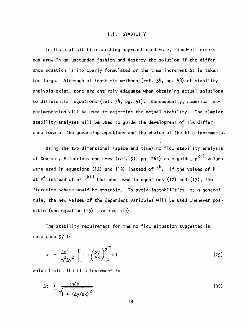
The stability requirement for the no flow situation suggested in

reference 37 is

=22 I + Ay (29) n2Ay2 AX

which limits the time increment to

At < "-mAy. (30)

;1+ (Ay/Ax)2

19

To account for Mach number, equation (30) is empirically modified to

At nAy(l - IMI) (31) I + (Ay/AX) 2

where the largest value of the local Mach number is used. Equation (31)

is used to set the initial time increment. If an instability should occur,­

the time increment will be reduced until stability occurs.

20

IV. STEADY STATE PRESSURES

In the sample problems to be presented in the next section, the time

dependent results will be compared to the results,of the steady harmonic

solutions of reference 10. The purpose of this section is to show the

rationale for constructing a steady state sol'utton from the time dependent

results.

A. Steady Harmonic Solution

The steady harmonic pressure ps(x,y) isdefined as a solution to

equations (l) to (3)when the pressure is assumed to be a simple harmonic

function of time:

P(x,y t) = ps(X,y)e t (32)

In this case where the source is a' simple harmonic function of time, ps

represents the Fourier transform of p(x,y,t) (ref0 28, pg. 11).

For a semi-infinite duct (or an equivalent finite duct with a-p c

exit impedance) with plane wave propagation, uniform Mach number, and hard

walls,, the solution for ps is (ref. 10, eq. (18))

- i2Tmx

Ps = eT(+M) (33)

In the next section, a transient solution to this problem will be compared

to equation (33).

21

B. Transient Times

Recall, at the start of the numerical calculations, the aioustic

pressures and velocities were assumed zero throughout the duct. Then,

a pressure source begins a harmonic oscillation at x=0 fort greater

than zero. For the special case of a plane wave propagation without

flow in a hard wall semi-infintte duct, the analytical solution to the

wave equation indicates that the transient solution ends and the steady

solution ps begins when (ref. 38, pg. 305)

tt > nx (34)

or in terms of real variable when

> x-/c o (35)t 0

The transient time in equations (34) and (35) represents the time for

the wave to travel down to the end of the duct, x = L

The transient time can be shortened or expanded depending on the

direction-of the flow and the transverse velocity distribution. In

genera-, the length of time for the transient-to occur will be found by

a trial numerical procedure. For the simple case of plug flow, equation

(34) is now modified to include a uniform Mach number,

tt I + M > ox (36)

Therefore, for the special case of one-dimensional plane wave propagation,

the initial transient is assumed to pass when equation (36) holds. As a

22

factor of-safety in the present calculationsi the transient calculation

will be continued into. the steady domain for one period of oscillation

before the Fourier pressure p is calculated. Therefore, in this paper

tc ij-H TI +

+ 1 +M

(37)

and

p(xy),= P(x,y,t)

ei27rtc

(38)

For more complicated problems, such as with higher order modes,

where reflections are important, or where complicated flow gradients

exist, t should be increased in successive steps to check for conver­c

gence.

23

V. SAMPLE CALCULATIONS

In the sample problems to follow, the time dependent results will

be compared to the analytical results of equation (33) and the steady

harmonic numerical solutions of reference (10).

A. Hard-Wall Duct

Numerical and analytical values of the pressure p(x,y) are computed

=for the case of a hard-wall duct for plane wave propagation with

exit impedance (equivalent to a semi-infinite duct) for no flow and plug

flow with Mach numbers of -0.5 and +0.5. The calculations are made with

a length to height ratio (L"/H") of I and a dimensionless frequency T1

of 1. The analytical and numerical values of the acoustic pressure pro­

files along the duct are shown in Figures 3, 4, and 5. As seen in these

figures, the agreement between the analytical-and numerical, theory is

reasonably good.

Some inaccuracy exists in the pressure at the entrance (x = 0). As

seen in Figures 3 and 4, the pressure at the second grid location takes

a slight jump. This is believed to result because the approximations

for the spatial derivatives are only first order at the corners. Future

work should be concerned with developing higher order difference approxi­

mations which are more accurate and stable. Higher order difference

would also be desirable in order to increase the mesh spacing used in

these calculations, and thereby reduce the number of grid points.

24

I

B. Soft-Wall Ducts

As another example of the time dependent analysis, the pressure

distribution was computed for the case of plane wave propagation with­

out steady flow and with a e = I exit impedance and a wall with

impedance value of 0.16 - 1 0.34. The calculation was made with a

length to height ratio of 0,5 and a dimensionless frequency of 0.6.

The results of the time dependent analysis along with the results of

the solution of the equivalent steady state Helmholtz equation are dis­

played in Figure 6. The numerical results for the steady spatial solu­

tion ps(x,y) are tabulated in Appendix F of reference 100

Again, as seen in Figure 6, the steady state and time dependent

solutions are in reasonable agreement. Hopefully, the difference be­

tween both theories-can be resolved by using higher order difference

approximations.

C. Grid Point Variations

Figure 7 shows the effect of increasing the number of grid points

on the computational time of the time dependent approach for the hard

wall duct associated with Figure 3. Roughly, as seen in Figure 4, the

computational time is proportional to the number of grid points used.

This is considerable advantage over the steady state technique inwhich

the computational time more nearly increases with the square of the

total grid points.

25

Figure 8 shows a comparison of the computational times for the

steady state and time dependent problems associated with the hard,wail.

duct shown in Figure 2. For this no-flow example, the continuity and

momentum equations, (1) to (3), can be combined into a single wave

equation

--2 = a--2 + 32 2 (39)

at Dx Dy

The time dependent solution to equation (39) was presented in reference,

37 and is represented by the lowest line in Figure 8.-

As seen in Figure 8 for J = 20, the time dependent analysts pre­

sented herein is roughly equal to the steady state analysis. The value

of J (grid points in y-direction) was restricted to 20 because of prac­

tical limitations on the size of the matrix which could be effectively

handled in the steady state analyst-s. When J was increased to 50 wi.th

50 axial grid points, the steady state analysis required 5500 seconds as

compared to less than 150 seconds for the time dependent analysis. This

large increase-in the steady state solution time results because of the

manner in which the general matrix was partitioned (ref. 10, pg. 14).

In this case, the storage and computational times are proportional to the

total number of transverse grid points squared.

As seen in Figure 8, the time dependent solutions for the-continuity

and momentum formulation in this paper require computational times a fac­

tor of 10 greater than the transient solution times to the wave equation

26

for the same degree of accuracy. This results- because much smaller time

increments At must be taken with the cont-inuity and momentum solutions

to obtain the same accuracy or truncation error. In the numerical formu­

lation of the wave equation (eq. (39)), the second derivative of time is

expressed in terms of the usual central difference approximation:

pk+] - 2Pk . + Pk-. - '' 'J + O(At 2 ) (40­

2 where the truncation error is of order At2. On the other hand, in the

continuity equation (eq. (11)), the first derivative of time is expressed

as a forward di-fference

.k+l pk9 P "- r. - P Il I + O(At)1,J (41)

at At

where the truncation error is of order At. Consequently, a numerical

solution based on equation (41) will require smaller time steps for the

same degree of accuracy.

D. Shear Flow

Although the shear flow difference equations have been programmed,

at the present time shear flow example problems have not been examined,

27

CONCLUSIONS

A time dependent two-dimensional .explicit numerical procedure was­

developed for the parallel sheared mean flow form of the separate con­

tinuity and momentum equations. This time marching technique was found

to be stable for both no flow and plug flow. At the present time, shear

flow examples have not been attempted. A special wall boundary condi­

tion was developed to insure stability for the soft wall case.

With the possible exception of the wave envelope technique (ref.

10) or the spatial marching technique (ref. 18), the numerical time de­

pendent method of analysis represents-a significant advance over previous

steady numerical theories. By eliminating large matr-ix storage require­

ments, numerical calculations of high sound frequencies are now possible.

Because manipulation of matrices is omitted, the time dependent approach

is much easier to program and debug0

28

REFERENCES

1. K. J. Baumeister and E. C. Bittner, "Numerical Simulation of Noise

Propagation in Jet Engine Ducts," NASA TN D-7339 (1973).

2. K. J. Baumeister and E. J. Rice, "A Difference Theory for Noise

Propagation in an Acoustically Lined Duct with Mean Flow," in

Aeroacoustics: Jet and Combustioi Noise; Duct Acoustics, edited by

H. T. Nagamatsu, J. V. O'Keefe, and I..R. Schwartz, Progress in

Astronautics and Aeronautics Series, Vol 37 (American Institute of

Aeronautics and Astronautics, New York, 1975), pp. 435-453.

3. K. J. Baumeister, "Analysis of Sound Propagation in Ducts Using the

Wave Envelope Concept," NASA TN D-7719 (1974).

4. D. W. Quinn, "A Finite Difference Method for Computing Sound Propa­

gation in Nonuniform Ducts," AIAA Paper No. 75-130 (January 1975).

5. K. J. Baumeister, "Wave Envelope Analysis of Sound Propagation in

Ducts with Variable Axial Impedance," in Aeroacoustics: Duct Acous­

tics, Fan Noise and Control Rotor Noise, edited by 1. R. Schwartz,

H. T. Nagamatsu, and W. Strahle, Progress in Astronautics and Aero­

nautics Series, Vol. 44 (American Institute of Aeronautics and Astro­

nautics, New York, 1976), pp. 45r-474.

6. D. W. Quinn, "Attenuation of Sound Associated with a Plane Wave i'n

a Multisectional Duct," in Aeroacoustics: " Duct Acoustics, Fan Noise

and Control Rotor Noise, edited by I[.R. Schwartz, H. T. Nagamatsu,

and W. Strahle, Progress in Astronautics and Aeronautics Series, Vol'.

44 (American Institute of Aeronauti-cs and Astronautics, New York,

1976), pp. 331-345.

29

7. R. K. Sigman, R. K. Majjigi, and B. T. Zinn, "Determination of

Turbofan Inlet Acoustics using Finite Elements,." AlAA 16, pp.

1139-1145 (1978).

8. A.- L. Abrahamson, "A Finite Element Algorithm for Sound Propaga­

tion in Axisymmetric Ducts Containing Compressible Mean Flow,"

NASA CR-145209 (June 1977).

9% A. Craggs, "A Fin.ite Method for Modelling Dissipative Mufflers.

With a Locally Reactive Linning," Sound Vibo 54, pp. 285-296

(1977).

10. K. J. Baumeister, "Finite-Difference Theory for Sound Propaga­

tion in a Lined Duct with Uniform Flow Using the Wave Envelope.

Concept," NASA TP-1O01 (1977).

11. Y. Kagawa, T. Yamabuchi, and A. Mori, "Finite Element Simulation

of an Ax!symmetric Acoustic Transmission System-with a Sound

Absorbing Wall," Sound Vib. 53, pp. 357-374 (1977).

12. W. Eversman, R. J. Astley, and V. P. Thanh, "Transmission in Non­

uniform Ducts - A Comparative Evaluation of Finite Element and

Weighted Residuals Computational Schemes," AIAA Paper No. 77­

1299 (October 1977).

13. R. Watson, "A Finite Element Simulation of Sound Attenuation in

a Finite Duct With a Peripherally Variable Liner," AIAA Paper No,

77-1300 (October 1977).

14. A. L. Abrahamson, "A Finite Element Algorithm for Sound Propaga­

tion in Axisymmetric Ducts Containing Compressible Mean Flow,"

AIAA Paper No. 77-1301 (October 1977).

30

15. K. J. Baumeister, "Numerical Spatial Marching Techniques for Esti­

mating Duct Attenuation and Source Pressure Profiles,!' in 95th

Meeting of the Acoustical Society of Anierica, Providence, R.I.-,

(May 16-19, 1978), also published as NASA TM-78857 (1978).

16. I. A. Tag and E. Lumsdaine, "An Effi'cient Finite Element Technique

for Sound Propagation in Axisymmetric Hard WalI Ducts Carrying High

Subsonic Mach Number Flows,'" AIAA Paper No. 78-1154 (July 1978).

17. R. J. Astley and W. Eversman, "A Finite Element Method for Trans­

mission inNon-Uniform Ducts wi.thout Flow: Comparison with th.e

Method of Weighted Residuals,)' Sound VibO 57, pp. 367-388 (1978).0

18.- K. J. Baumeister, "Numerical Spatial Marching Techniques in Duct-

Acoustics," J. Acoust. Soc.. Am. 65, pp. 297-306 (1979).

19. R. K. Majj'igi, "Application of Finite Element Techniques in Pre­

dicting the Acoustic Properties of Turbofan Inlets," Ph. D. Thesis,

Georgia Institute of Technology, Atlanta, GA, (1979).

20. K. J. Baumeister, 'Optimized Multisectioned Acoustic Liners,"

AIAA Paper No. 79-0182 (January 1979).

21. R. K. Majjigi, R. K. Sigman, and B. T. Zinn, "Wave Propagation in,

Ducts Using the Finite Element Method," AIAA Paper No, 79-0659

(March 1979).

22. R. J. Astley and W. Eversman, "The Application of Finite Element

Techniques to Acoustic Transmission in Lined Ducts with Flow,"

AIAA Paper No. 79-0660 (March 1979).

23. D. W. Quinn, "A Finite Element Method for Computing Sound Propaga­

tion in Ducts Containing Flow," AIAA Paper No. 79-0661 (March 1979).

31

24. A. L. Abrahamson, "Acoustic Duct Liner Optimization Using Finite

Elements," AIAA Paper No. 7.9-0662 (March 1979).

25. I. A. Tag and J. E. Akin, "Finite Element.Solution of Sound Prop­

agation in a Variable Area Duct," AIAA Paper No. 79-0663 (March

1979).

26. H. C. Lester and T. L. Parrott, "Application of Finite Element

Methodology for Computing Grazing Incidence Wave Structure in an

Impedance Tube: Comparison with Experiment," AIAA Paper No. 79­

0664 (March 1979).

27. K. J. Baumeister and R. K. Majjigi, "Applications of the Velocity

Potential Function to Acoustic Duct Propagation and Radiation

from Inlets Us.ing Finite Element Theory," AIAA Paper No. 79-0680

(March 1979).

28. M. E. Goldstein, Aeroacoustics, (McGraw-Hill, New York, 1976).

29. M. J. Beaubien and A. Wexler, "Iterative, Finite Difference Solu­

tion of Interior Eigenvalues and Eigenfunctions of Laplace's

Operator, " The Computer J.-14, pp. 263-269 (1971).

30. B. T. Browne and P. J. Lawrenson, 'Numerical Solution of an El­

liptic Boundary-Value Problem in the Complex Variable," J. Inst.

Maths. Applics. 17, pp. 311-327 (1976).

31. R. D. Richtmyer and K. W. Morton, Difference Methods for Initial-

Valve Problems, (Interscience Publishers, New York, 1967), 2nd ed.

32. P. Fox, "The.Solution of Hyperbolic Partial Differential Equations

by Difference Methods," in Mathematical Methods for Digital Com­

puters, edited by A. Ralston and H. S. Wilf (John Wiley, Mew York,

1960), Vol. 1, pp. 180-188.

32

33. C. F. Gerald, Applied Numerical Analysisj (Addison-Wesley, Reading,

MA, 1978), 2nd ed.

34. P. J. Roache, Computational Fluid Dynamics, (Hermosa, Alburquerque,

N. M.-, 1972).

35. M. Clark and K. F. Hansen, Numerical Methods of Reactor Analys-is,

(Academic Press, New York, 1964)..

36. F. B. Hildebrand, Methods of Applied Mathematics, (Prentice-Hall,

New Jersey, 1952).

37. K. J. Baumeister, "Time Dependent Difference Theory for Noise Propaga­

tion in Jet Engine Ducts," AIAA Paper No. 80-0098, to be presented

AIAA 18th Aerospace Sciences Meeting, Pasadena, CA, (January 14-16,

1980).

38. B. M. Budak; A. A. Samarski, and A. N. Tikhonov, A Collection of Prob­

lems on Mathematical Physics, (Pergamon Press, Oxford, 1964).

33

INIT[AL-CONDITION GRID POINTS - a 0 aea 6 a EXIT

o * * o 0 0 0 0 PLANE SOURCE * , * 0 * PLANE- (i-I,]) (I) i .j)

00 0 0 0(ia 1)l

SPECIFIC ACOUSTIC WALL IMPEDANCE

Figure . - Grid-point representation of two-dimensional flow duct

INftIAL-CONDITI]ON GRID POINTS---- 0 6 0 0 rEXF

* PLANESOURCE

PLANE 0 0 0, 0 a 0 1 * 0 0 * 0 6 0 1

SPECIFIC ACOUSTIC WALL IMPEDANCE C,

Figure 2. - Grid-point representation of two­dimensional flow duct using pressure boundarycondition at walls.

TIME DEPENDENI NUMERICAL RESULTS o REAL PART p(1) TIME DEPENDENT NUMERICAL RESULTS 0 IMAGINARY PART p0 1 REAL PART p(1)

0 IMAGINARY PART p(2) EXACT ANALYSIS, eq(33)

REAL PART, p (1) EXACT ANALYSIS, eq(33)(2) IMAGINARY PART ps REAL PART, p (1)

PLANE HARD WALL-% IMAGINARR HARD WALL PRESSURE I I WAVE JGRID POINTS -0PLANE = PAE ----­jO

PRESSURE 0X a~ VAVt-W x

1/+1 04

0-. U)

- U)"

0-I .­i1.­

0 El Af , 00 0 0II Ol

0 .

inahadwal duc . 01, , H:foy=,' n I IDIMENSIONLESS AXIAL COORDINATES, x

0 .51, DIMENSIONLESS AXIAL COORDINATE, x Figure 4A- Analytical and numerical pressure profiles

for one-dimensional plane wave sound propagationFigure 3. - Analytical and numerical pressure profiles in a hard wall duct for IA= +05, 71=1, and

for one-dimensional plane wave sound propagation VIK-1_ = I1(I - 25, J m10, At = 0.002438).in a hard wall duct for M-0, 71 1, and l{'/W1 I (I -25, i 20, At = 0.004084).

TIME DEPENDENT NUMERICAL RESULTS

O REAL PART, p(1) O IMAGINARY PART, p(2)

EXACT ANALYSIS, eq(33) REAL PART, Ps( )

(2) IMAGINARY PART, pS

HARD WALL,,

PLANE PRESSURE JM ,,5 1 WAVE- x

1.0

=" "l

_0­

,

Wplane E- L

I-lO.5 1.0

DIMENSIONLESS AXIAL COORDINATES, x

Figure 5. - Analytical and numerical pressure profiles for one-dimensional plane wave sound propagation in a hard wall duct for M = -0.5, 71= 1, and L([H* = 1 (I - 49, J = 1O, At =Q00064).

0 TIME DEPENDENT NUMERICAL LO [ ___

STEAD STATSTATE FSTEADYFINITE DIFFERENCE SOLUTION, ref 10, PROB# I

PLANEPRESSURE .5 WV,

DIMENSIONLESS AXIAL COORDINATE, x

Figure 6. - Pressure magnitude on the duct axis for incident wave sound propagation in a soft wall duct (M= 0,

=70.6, L*N m=.5, =0. 16 - iO. 3, 1 = 6, 1 = 10,

At .0056).

1000 TRANSIENT SOLUTION (CONTINUITY AND MOMENTUM,

100 [-- a = a0156) TRANSVERSE GRID

POINTS J 0)

20

_J 10 Pgi10

,-I ­

< 10 /STEADY STATE SOLUTION

.00

0 20 40 60 80 100 120 '-TRANSIENT SOLUTION NUMBER OF AXIAL GRID POINTS, I, T/(WAVE EQUATION, C= 1)

Figure 7. - Effect of increasing number of grid points /E

on calculational time of transient solution for plane wave propagation in a hard wall duct (M= 0, 71= 1, 2 0/- * = 1, and a = 1). 0 20 40 60 80 100 120

NUMBER OF AXIAL GRID POINTS, I

Figure 8. - Comparison of transient and steady state calculations for plane wave propagation in a hard wall duct (M m0, 7 = 1, L/H4 = 1, J = 20).

fleport No j 2 Government Accession No. 3 Recipient's Catalog No NASA TM-79302 I

4 Title and Subtitle

A TIME DEPENDENT DIFFERENCE THEORY FOR S

PROPAGATION IN DUCTS WITH FLOW

5. Report Date

OUND 6 Performing Organization Code

7 Author(s) 8

K. J. Baumeister 10

9. Performing Organization Name and Address

National Aeronautics and Space Administration 11.

Lewis Research Center

Performing Organization Report No

E-254

Work Unit No

Contract or Grant No

Cleveland, Ohio 44135 13 Type of Report and Period Covered

12. Sponsoring Agency Name and Address

National Aeronautics and-Space Administration

Washington, D. C. 20546 14

Technical Memorandum

Sponsoring Agency Code

15. Supplementary Notes

16 Abstract

A time dependent numerical solution of the linearized continuity and momentum equation is

developed for sound propagation in a two-dimensional straight hard or soft wall duct with a

sheared mean flow. The time dependent governing acoustic-difference equations and boundary

conditions are developed along with a numerical determination of the maximum stable time in­

crements. The analysis begins with a harmonic noise source radiating into a quiescent duct.

This explicit iteration method then calculates stepwise in real time to obtain the transient as

well as the "steady" state solution of the acoustic field. Example calculations are presented

for sound propagation in hard and soft wall ducts, with no flow and with plug flow. Although

the problem with sheared flow has been formulated and programmed, sample calculations have

not yet been examined. So far, the time dependent finite difference analysis has been found to

be superior to the steady state finite difference and finite element techniques because of shorter

solution times and the elimination of large matrix storage requirements.

17. Key Words (Suggested by Author(s)) 18. Distribution Statement

Finite difference Unclassified - unlimited

Time dependent STAR Category 71

Linear acoustics

19. Security classif. (of this report) 20 Security Classif. (of this page) 21. No of Pages 22. Price

Unclassified Unclassified I

sale by the National Technical Information Service, Springfield, Virginia 22161*For

20546

National Aeronautics and SPECIAL FOURTH CLASS MAIL Postage and Fees Paid Space Administration BOOK National Aeronautics andSpaceAdmiistrtionSpace Administration

NASA-451 Washington, D.C.

Official Business Penalty for Private Use, $300

aPOSTMASTER: 1 8If Undeliverable (Section Manual) Do Not ReturnPJASAPostal