Embed Size (px)
Citation preview

POLITECNICO DI MILANODEPARTMENT OF MATHEMATICS
DOCTORAL PROGRAMME IN
MATHEMATICAL MODELS AND METHODS IN ENGINEERING
ASYMPTOTIC ANALYSIS OF EVOLUTIONEQUATIONS WITH NONCLASSICAL
HEAT CONDUCTION
Doctoral Dissertation of: FILIPPO DELL’ORO
Advisor: Prof. VITTORINO PATA
Tutor: Prof. DARIO PIEROTTIChair of the PhD Program: Prof. ROBERTO LUCCHETTI
CYCLE XXVI

Summary
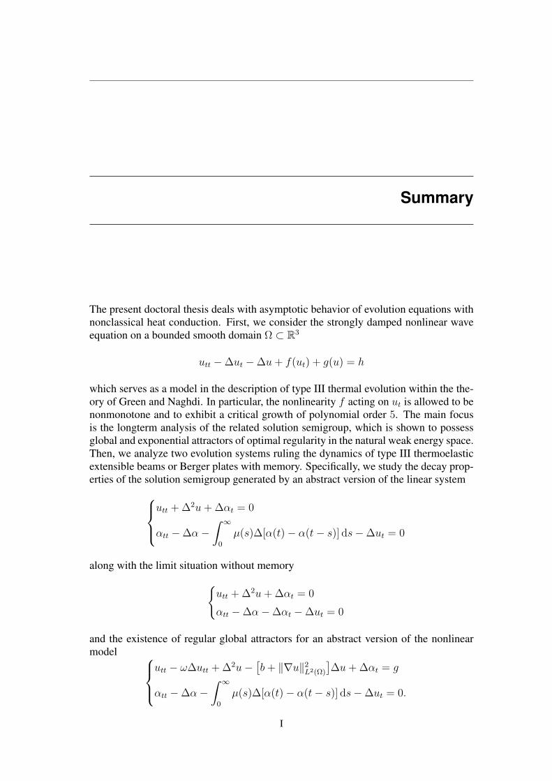
The present doctoral thesis deals with asymptotic behavior of evolution equations withnonclassical heat conduction. First, we consider the strongly damped nonlinear waveequation on a bounded smooth domain Ω ⊂ R3
utt −∆ut −∆u+ f(ut) + g(u) = h
which serves as a model in the description of type III thermal evolution within the the-ory of Green and Naghdi. In particular, the nonlinearity f acting on ut is allowed to benonmonotone and to exhibit a critical growth of polynomial order 5. The main focusis the longterm analysis of the related solution semigroup, which is shown to possessglobal and exponential attractors of optimal regularity in the natural weak energy space.Then, we analyze two evolution systems ruling the dynamics of type III thermoelasticextensible beams or Berger plates with memory. Specifically, we study the decay prop-erties of the solution semigroup generated by an abstract version of the linear system
utt +∆2u+∆αt = 0
αtt −∆α−∫ ∞
0
µ(s)∆[α(t)− α(t− s)] ds−∆ut = 0
along with the limit situation without memoryutt +∆2u+∆αt = 0
αtt −∆α−∆αt −∆ut = 0
and the existence of regular global attractors for an abstract version of the nonlinearmodel
utt − ω∆utt +∆2u−[b+ ∥∇u∥2L2(Ω)
]∆u+∆αt = g
αtt −∆α−∫ ∞
0
µ(s)∆[α(t)− α(t− s)] ds−∆ut = 0.
I

Moreover, we discuss the asymptotic behavior of the nonlinear type III Caginalp phase-field system
ut −∆u+ ϕ(u) = αt
αtt −∆αt −∆α + g(α) = −ut
on a bounded smooth domain Ω ⊂ R3, with nonlinearities ϕ and g of polynomialcritical growth 5, proving the existence of the regular global attractor. Finally, weanalyze the linear differential system
ρ1φtt − κ(φx + ψ)x = 0
ρ2ψtt − bψxx + κ(φx + ψ) + δθx = 0
ρ3θt −1
β
∫ ∞
0
g(s)θxx(t− s) ds+ δψtx = 0
describing a Timoshenko beam coupled with a temperature evolution of Gurtin-Pipkintype. A necessary and sufficient condition for exponential stability is established interms of the structural parameters of the equations. In particular, we generalize pre-viously known results on the Fourier-Timoshenko and the Cattaneo-Timoshenko beammodels.
In the first chapter of the thesis we introduce some preliminary results about infinite-dimensional dynamical systems and linear semigroups needed in the course of the in-vestigation. The remaining chapters correspond to the following papers, written duringthe three years of PhD.
• F. Dell’Oro and V. Pata, Long-term analysis of strongly damped nonlinear waveequations, Nonlinearity 24 (2011), 3413–3435, (Chapter 2 and Chapter 3).
• F. Dell’Oro and V. Pata, Strongly damped wave equations with critical nonlinear-ities, Nonlinear Anal. 75 (2012), 5723–5735, (Chapter 4).
• F. Dell’Oro, Global attractors for strongly damped wave equations with sub-critical-critical nonlinearities, Commun. Pure Appl. Anal. 12 (2013), 1015–1027, (Chapter 5).
• M. Coti Zelati, F. Dell’Oro and V. Pata, Energy decay of type III linear thermoe-lastic plates with memory, J. Math. Anal. Appl. 401 (2013), 357–366, (Chapter 6).
• F. Dell’Oro and V. Pata, Memory relaxation of type III thermoelastic extensiblebeams and Berger plates, Evol. Equ. Control Theory 1 (2012), 251–270, (Chap-ter 6).
• M. Conti, F. Dell’Oro and A. Miranville, Asymptotic behavior of a generaliza-tion of the Caginalp phase-field system, Asymptot. Anal. 81 (2013), 297–314,(Chapter 7).
• F. Dell’Oro and V. Pata, On the stability of Timoshenko systems with Gurtin-Pipkin thermal law, submitted, (Chapter 8).
II

Acknowledgments
I thank my advisor Prof. Vittorino Pata for introducing me to the fascinating field ofinfinite-dimensional dynamical systems, and for the competence, enthusiasm, profes-sionality and constant guidance during these three years of PhD.
I also thank Prof. Monica Conti for the interest, help and several remarkable teach-ings, and Prof. Jaime Munoz Rivera for the kind hospitality in Petropolis and manystimulating discussions.
I express my sincere gratitude to my family for the support and the quotidian encour-agement. I heartily thank Silvia for her love and her constant precious presence in mylife.
III

Contents
Introduction 1
1 Preliminaries 91.1 Infinite-Dimensional Dynamical Systems . . . . . . . . . . . . . . . . 9
1.1.1 Dissipative dynamical systems . . . . . . . . . . . . . . . . . . 91.1.2 Global and exponential attractors . . . . . . . . . . . . . . . . 111.1.3 Gradient systems . . . . . . . . . . . . . . . . . . . . . . . . . 13
1.2 Linear Semigroups . . . . . . . . . . . . . . . . . . . . . . . . . . . . 14
2 Strongly Damped Nonlinear Wave Equations 172.1 Introduction . . . . . . . . . . . . . . . . . . . . . . . . . . . . . . . 172.2 Preliminaries . . . . . . . . . . . . . . . . . . . . . . . . . . . . . . . 18
2.2.1 Notation . . . . . . . . . . . . . . . . . . . . . . . . . . . . . 182.2.2 General agreements . . . . . . . . . . . . . . . . . . . . . . . 192.2.3 A technical lemma . . . . . . . . . . . . . . . . . . . . . . . . 19
2.3 An Equivalent Formulation . . . . . . . . . . . . . . . . . . . . . . . 192.3.1 Decompositions of the nonlinear terms . . . . . . . . . . . . . 192.3.2 The equation revisited . . . . . . . . . . . . . . . . . . . . . . 212.3.3 The renormed spaces . . . . . . . . . . . . . . . . . . . . . . . 212.3.4 Formal estimates . . . . . . . . . . . . . . . . . . . . . . . . . 22
2.4 The Solution Semigroup . . . . . . . . . . . . . . . . . . . . . . . . . 222.4.1 Well-posedness . . . . . . . . . . . . . . . . . . . . . . . . . . 222.4.2 Sketch of the proof . . . . . . . . . . . . . . . . . . . . . . . . 232.4.3 The semigroup . . . . . . . . . . . . . . . . . . . . . . . . . . 24
2.5 Dissipativity . . . . . . . . . . . . . . . . . . . . . . . . . . . . . . . 242.6 Partial Regularization . . . . . . . . . . . . . . . . . . . . . . . . . . 26
3 Attractor for the SDNWE. The Critical-Subcritical Case 293.1 Introduction . . . . . . . . . . . . . . . . . . . . . . . . . . . . . . . 293.2 The Global Attractor . . . . . . . . . . . . . . . . . . . . . . . . . . . 303.3 A Conditional Result . . . . . . . . . . . . . . . . . . . . . . . . . . . 32
V

Contents
3.4 Regularity of the Attractor . . . . . . . . . . . . . . . . . . . . . . . . 33
4 Attractor for the SDNWE. The Fully-Critical Case 374.1 Introduction . . . . . . . . . . . . . . . . . . . . . . . . . . . . . . . 374.2 The Dissipative Dynamical System . . . . . . . . . . . . . . . . . . . 38
4.2.1 Dissipative estimates . . . . . . . . . . . . . . . . . . . . . . . 394.2.2 The dissipation integral . . . . . . . . . . . . . . . . . . . . . 39
4.3 Global and Exponential Attractors . . . . . . . . . . . . . . . . . . . . 404.3.1 Statement of the result . . . . . . . . . . . . . . . . . . . . . . 404.3.2 Proof of Theorem 4.3.1 . . . . . . . . . . . . . . . . . . . . . 40
4.4 Proof of Lemma 4.3.1 . . . . . . . . . . . . . . . . . . . . . . . . . . 424.5 Proof of Lemma 4.3.2 . . . . . . . . . . . . . . . . . . . . . . . . . . 464.6 Proof of Lemma 4.3.3 . . . . . . . . . . . . . . . . . . . . . . . . . . 47
5 Attractor for the SDNWE. The Subcritical-Critical Case 515.1 Introduction . . . . . . . . . . . . . . . . . . . . . . . . . . . . . . . 515.2 The Global Attractor . . . . . . . . . . . . . . . . . . . . . . . . . . . 535.3 Regularity of the Attractor . . . . . . . . . . . . . . . . . . . . . . . . 56
6 Extensible Beams and Berger Plates 616.1 Introduction . . . . . . . . . . . . . . . . . . . . . . . . . . . . . . . 616.2 Functional Setting and Notation . . . . . . . . . . . . . . . . . . . . . 636.3 The Solution Semigroup . . . . . . . . . . . . . . . . . . . . . . . . . 65
6.3.1 The past history formulation . . . . . . . . . . . . . . . . . . . 656.3.2 Well-posedness . . . . . . . . . . . . . . . . . . . . . . . . . . 65
6.4 The Main Result . . . . . . . . . . . . . . . . . . . . . . . . . . . . . 666.5 Further Remarks . . . . . . . . . . . . . . . . . . . . . . . . . . . . . 676.6 The Lyapunov Functional . . . . . . . . . . . . . . . . . . . . . . . . 696.7 An Auxiliary Functional . . . . . . . . . . . . . . . . . . . . . . . . . 696.8 Dissipation Integrals . . . . . . . . . . . . . . . . . . . . . . . . . . . 716.9 Proof of Theorem 6.4.1 . . . . . . . . . . . . . . . . . . . . . . . . . 73
6.9.1 Conclusion of the proof of Theorem 6.4.1 . . . . . . . . . . . . 776.10 Proofs of Proposition 6.4.1 and Corollary 6.4.2 . . . . . . . . . . . . . 78
6.10.1 Proof of Proposition 6.4.1 . . . . . . . . . . . . . . . . . . . . 786.10.2 Proof of Corollary 6.4.2 . . . . . . . . . . . . . . . . . . . . . 78
6.11 The Linear Case . . . . . . . . . . . . . . . . . . . . . . . . . . . . . 796.12 The Contraction Semigroups . . . . . . . . . . . . . . . . . . . . . . 79
6.12.1 The first system . . . . . . . . . . . . . . . . . . . . . . . . . 806.12.2 The second system . . . . . . . . . . . . . . . . . . . . . . . . 81
6.13 Decay Properties of the Semigroup U1(t) . . . . . . . . . . . . . . . . 836.14 Decay Properties of the Semigroup U2(t) . . . . . . . . . . . . . . . . 86
7 Caginalp Phase-Field Systems 897.1 Introduction . . . . . . . . . . . . . . . . . . . . . . . . . . . . . . . 897.2 Preliminaries . . . . . . . . . . . . . . . . . . . . . . . . . . . . . . . 90
7.2.1 Functional setting . . . . . . . . . . . . . . . . . . . . . . . . 907.2.2 Technical lemmas . . . . . . . . . . . . . . . . . . . . . . . . 91
VI
Contents
7.3 The Solution Semigroup . . . . . . . . . . . . . . . . . . . . . . . . . 937.4 A Priori Estimates and Dissipativity . . . . . . . . . . . . . . . . . . . 957.5 Further Dissipativity . . . . . . . . . . . . . . . . . . . . . . . . . . . 977.6 The Global Attractor . . . . . . . . . . . . . . . . . . . . . . . . . . . 100
8 Timoshenko Systems with Gurtin-Pipkin Thermal Law 1038.1 Introduction . . . . . . . . . . . . . . . . . . . . . . . . . . . . . . . 103
8.1.1 The Fourier thermal law . . . . . . . . . . . . . . . . . . . . . 1048.1.2 The Cattaneo thermal law . . . . . . . . . . . . . . . . . . . . 1048.1.3 The Gurtin-Pipkin thermal law . . . . . . . . . . . . . . . . . . 105
8.2 Comparison with Earlier Results . . . . . . . . . . . . . . . . . . . . 1068.2.1 The Fourier case . . . . . . . . . . . . . . . . . . . . . . . . . 1068.2.2 The Cattaneo case . . . . . . . . . . . . . . . . . . . . . . . . 1078.2.3 The Coleman-Gurtin case . . . . . . . . . . . . . . . . . . . . 1078.2.4 Heat conduction of type III . . . . . . . . . . . . . . . . . . . 108
8.3 Functional Setting and Notation . . . . . . . . . . . . . . . . . . . . . 1098.3.1 Assumptions on the memory kernel . . . . . . . . . . . . . . . 1098.3.2 Functional spaces . . . . . . . . . . . . . . . . . . . . . . . . 1098.3.3 Basic facts on the memory space . . . . . . . . . . . . . . . . 110
8.4 The Contraction Semigroup . . . . . . . . . . . . . . . . . . . . . . . 1108.5 Some Auxiliary Functionals . . . . . . . . . . . . . . . . . . . . . . . 113
8.5.1 The functional I . . . . . . . . . . . . . . . . . . . . . . . . . 1138.5.2 The functional J . . . . . . . . . . . . . . . . . . . . . . . . . 1148.5.3 The functional K . . . . . . . . . . . . . . . . . . . . . . . . 1158.5.4 The functional L . . . . . . . . . . . . . . . . . . . . . . . . . 116
8.6 Proof of Theorem 8.1.1 (Sufficiency) . . . . . . . . . . . . . . . . . . 1178.6.1 A further energy functional . . . . . . . . . . . . . . . . . . . 1178.6.2 Conclusion of the proof of Theorem 8.1.1 . . . . . . . . . . . . 117
8.7 Proof of Theorem 8.1.1 (Necessity) . . . . . . . . . . . . . . . . . . . 1188.8 More on the Comparison with the Cattaneo Model . . . . . . . . . . . 120
Appendix 123
Conclusions 129
Bibliography 130
VII


Introduction
The aim of the research contained in the present doctoral thesis is the mathematicalanalysis of well-posedness and asymptotic behavior of linear and nonlinear dissipativepartial differential equations with nonclassical heat conduction, that is, thermal evolu-tions where the temperature may travel with finite speed propagation. In the linear case,we mainly focus on the stability properties of the associated semigroups, analyzing thedecay to zero of the solutions. In the nonlinear situation, we dwell on existence andregularity of finite-dimensional global and exponential attractors, providing a completedescription of the asymptotic dynamics by means of suitable “small” regions of thephase space.
Hereafter is a detailed discussion of the models considered in the thesis. In particular,the nonclassical character of the temperature is stressed and the physical meaning andrelevance are explained.
Nonlinear Heat Conduction of Type III
Let Ω ⊂ R3 be a bounded domain with sufficiently smooth boundary ∂Ω. The thermalevolution in a homogenous isotropic (rigid) heat conductor occupying the space-timecylinder ΩT = Ω× (0, T ) is governed by the balance equation
et + div q = F.
Here, the internal energy e is a function of the relative temperature field
ϑ = ϑ(x, t) : ΩT → R,
that is, the temperature variation from an equilibrium reference value, while
q = q(x, t) : ΩT → R3
is the heat flux vector. Finally, F represents a source term. We also assume the Dirichletboundary condition
ϑ(x, t)|x∈∂Ω = 0,
1

Introduction
expressing the fact that the boundary ∂Ω of the conductor is kept at null (i.e. equilib-rium) temperature for all times. Considering only small variations of ϑ and ∇ϑ, theinternal energy fulfills with good approximation the equality
e(x, t) = e0(x) + cϑ(x, t),
where e0 is the internal energy at equilibrium and c > 0 is the specific heat. Accord-ingly, the balance equation becomes
cϑt + div q = F. (1)
For a general F of the form
F (x, t) = −f(ϑ(x, t)) + h(x), (2)
accounting for the simultaneous presence of a time-independent external heat supplyand a nonlinearly temperature-dependent internal source, equation (1) reads
cϑt + div q+ f(ϑ) = h. (3)
To complete the picture, a further relation is needed: the so-called constitutive law forthe heat flux, establishing a link between q and ϑ. In fact, the choice of the constitutivelaw is what really determines the model. At the same time, being a purely heuristicinterpretation of the physical phenomenon, it may reflect different individual percep-tions of reality, or even philosophical beliefs. For instance, for the classical Fourierconstitutive law
q+ κ∇ϑ = 0, κ > 0, (4)
we deduce from (3) the familiar reaction-diffusion equation
cϑt − κ∆ϑ+ f(ϑ) = h.
Nevertheless, such an equation predicts instantaneous propagation of (thermal) signals,a typical side-effect of parabolicity. This feature, sometimes called the paradox of heatconduction (see e.g. [14, 32]), has often encountered strong criticism in the scientificcommunity, up to be perceived as “physically unrealistic” by some authors. Therefore,several attempts have been made through the years in order to introduce some hyper-bolicity in the mathematical modeling of heat conduction (see e.g. [8, 48]). A possiblechoice is adopting the Maxwell-Cattaneo law [8], namely, the differential perturbationof (4)
q+ εqt + κ∇ϑ = 0, κ≫ ε > 0. (5)
In which case, the sum (3)+ε∂t(3) entails the hyperbolic reaction-diffusion equation
εcϑtt − κ∆ϑ+ [c+ εf ′(ϑ)]ϑt + f(ϑ) = h,
widely employed in the description of many interesting phenomena, such as chemi-cal reacting systems, gene selection, population dynamics or forest fire propagation,to name a few (cf. [33, 59, 60]). Another strategy is relaxing (4) by means of a time-convolution against a suitable (e.g. convex, decreasing and summable) kernel µ. Pre-cisely, omitting the dependence on x,
q(t) = −κ0∇ϑ(t)−∫ t
−∞µ(t− s)∇ϑ(s) ds. (6)
2
Introduction
The constant κ0 can be either strictly positive or zero, according to the models ofColeman-Gurtin [18] or Gurtin-Pipkin [48], respectively. Plugging (6) into (3) we endup with the integrodifferential equation
cϑt − κ0∆ϑ−∫ ∞
0
µ(s)∆ϑ(t− s) ds+ f(ϑ) = h.
Quite interestingly, in the (fully hyperbolic) case κ0 = 0, we recover (5) as the particu-lar instance of (6) corresponding to the kernel
µ(s) =κ
εe−s/ε.
In a different fashion, the theory of heat conduction of type III devised by Green andNaghdi [43–47, 90] considers instead a perturbation of the classical law (4) of integralkind. Indeed, the Fourier law is modified in the following manner:
q+ κ∇ϑ+ ω∇u = 0, κ, ω > 0, (7)
where an additional independent variable appears: the thermal displacement u : ΩT →R, defined as
u(x, t) = u(x, 0) +
∫ t
0
ϑ(x, s) ds,
hence satisfying the equality
ut(x, t) = ϑ(x, t), ∀ (x, t) ∈ ΩT ,
and (for consistency) complying with the Dirichlet boundary condition
u(x, t)|x∈∂Ω = 0.
Using (7) the balance equation (1) turns into
cutt − κ∆ut − ω∆u = F.
Replacing for more generality (2) with
F (x, t) = −f(ϑ(x, t))− g(u(x, t)) + h(x),
allowing the source term to contain a further contribution depending nonlinearly on thethermal displacement, we finally arrive at the boundary-value problem
cutt − κ∆ut − ω∆u+ f(ut) + g(u) = h,
u|∂Ω = 0,
ut|∂Ω = 0,
which will be analyzed in Chapters 2-5. We refer the reader to [80–87] for discussionsand other developments related to type III heat conduction.
3

Introduction
Type III Thermoelastic Extensible Beams and Berger Plates
For n = 1, 2, let Ω ⊂ Rn be a bounded domain with sufficiently smooth boundary ∂Ω.Given the parameters ω > 0 and b ∈ R, we consider the evolution system of coupledequations on the space-time cylinder Ω+ = Ω× R+
utt − ω∆utt +∆2u−[b+ ∥∇u∥2L2(Ω)
]∆u+∆ϑ = g, (8)
ϑt + div q−∆ut = 0, (9)
in the unknown variables
u = u(x, t) : Ω+ → R, ϑ = ϑ(x, t) : Ω+ → R, q = q(x, t) : Ω+ → Rn.
Such a system, written here in normalized dimensionless form, rules the dynamics ofa thermoelastic extensible beam (for n = 1) or Berger plate (for n = 2) of shape Ωat rest (see [4, 93]). Accordingly, the variable u stands for the vertical displacementfrom equilibrium, ϑ is the (relative) temperature and q is the heat flux vector obeyingsome constitutive law, depending on one’s favorite choice of heat conduction model.The term −ω∆utt appearing in the first equation witnesses the presence of rotationalinertia, whereas the real parameter b accounts for the axial force acting in the referenceconfiguration: b > 0 if the beam (or plate) is stretched, b < 0 if compressed. Finally,the function g : Ω → R describes a lateral load distribution. We also assume thatthe ends of the beam (or plate) are hinged, which translates into the hinged boundaryconditions for u
u(x, t)|x∈∂Ω = ∆u(x, t)|x∈∂Ω = 0,
and we take the Dirichlet boundary condition for ϑ
ϑ(x, t)|x∈∂Ω = 0,
expressing the fact that the boundary ∂Ω is kept at null (i.e. equilibrium) temperaturefor all times. It is worth noting that different boundary conditions for u are physicallysignificant as well, such as the clamped boundary conditions
u|∂Ω =∂u
∂ν
∣∣∣∂Ω
= 0,
where ν is the outer normal vector. However, the mathematical analysis carried outin this thesis (see Chapter 6) depends on the specific structure of the hinged boundaryconditions (the so called “commutative case”). In the clamped case major modificationson the needed tools are required and the proofs become much more technical.
We are left to specify the constitutive relation for the heat flux, establishing a linkbetween q and ϑ. Adopting for instance the classical Fourier law (the physical constantsare set to 1)
q = −∇ϑ,
equation (9) turns intoϑt −∆ϑ−∆ut = 0.
4

Introduction
In a different fashion, as already said, the theory of heat conduction of type III devisedby Green and Naghdi considers a perturbation of the classical law of integral kind, bymeans of the so-called thermal displacement
α(x, t) = α0(x) +
∫ t
0
ϑ(x, s) ds,
satisfying the equality αt = ϑ and (for consistency) complying with the Dirichletboundary condition
α(x, t)|x∈∂Ω = 0.
Then, the Fourier law is modified as
q = −∇αt −∇α,
so that (9) takes the form
αtt −∆α−∆αt −∆ut = 0. (10)
Still, the equation predicts infinite speed propagation of (thermal) signals, due to itspartially parabolic character which provides an instantaneous regularization of αt. Suchan effect is not expected (nor observed) in real conductors. Similarly to what donein [30] for the Fourier case, a possible answer is considering a memory relaxations ofthe above constitutive law of the form
q(t) = −∫ ∞
0
κ(s)∇αt(t− s) ds−∇α(t),
for some bounded convex summable function κ (the memory kernel) of total mass∫ ∞
0
κ(s) ds = 1.
Up to a rescaling, we may also suppose κ(0) = 1. Accordingly, (9) becomes
αtt −∆α−∫ ∞
0
κ(s)∆αt(t− s) ds−∆ut = 0, (11)
where the past history of the temperature is supposed to be known and regarded as aninitial datum of the problem. It is readily seen that, when the function κ converges inthe distributional sense to the Dirac mass at zero, equation (10) is formally recoveredfrom (11). From the physical viewpoint, this means that (10) is close to (11) when thememory kernel is concentrated, i.e. when the system keeps a very short memory of thepast effects. As a matter of fact, (11) can be given a more convenient form. Indeed,defining the differentiated kernel
µ(s) = −κ′(s),
a formal integration by parts yields∫ ∞
0
κ(s)∆αt(t− s) ds =
∫ ∞
0
µ(s)∆[α(t)− α(t− s)] ds.
5

Introduction
In summary, equation (8) and the particular concrete realization (11) of (9) give rise tothe system
utt − ω∆utt +∆2u−[b+ ∥∇u∥2L2(Ω)
]∆u+∆αt = g,
αtt −∆α−∫ ∞
0
µ(s)∆[α(t)− α(t− s)] ds−∆ut = 0,
which will be analyzed in Chapter 6 (actually, in a more general abstract form). Asa matter of fact, from the physical viewpoint, it is also relevant to neglect the effectof the rotational inertia on the plate (see e.g. [40, 51, 55, 57]). This corresponds to thelimit situation when ω = 0. Hence, we will also consider the following linear andhomogeneous version of the above model
utt +∆2u+∆αt = 0,
αtt −∆α−∫ ∞
0
µ(s)∆[α(t)− α(t− s)] ds−∆ut = 0,
along with the system utt +∆2u+∆αt = 0,
αtt −∆α−∆αt −∆ut = 0,
formally obtained when the memory kernel collapses into the Dirac mass at zero. Aswe will see, the presence of the memory produces a lack of exponential stability of theassociated linear semigroups, preventing the analysis of the asymptotic properties inthe nonlinear case.
Type III Nonlinear Caginalp Phase-Field Systems
Let Ω ⊂ R3 be a bounded domain with smooth boundary ∂Ω. The thermal evolution ofa material occupying a volume Ω, with order parameter u and (relative) temperature ϑ,is governed by the equations
∂u
∂t= −∂Ψ
∂u, (12)
∂H
∂t+ div q = F. (13)
Here, Ψ denotes the total free energy of the system defined as
Ψ(u, ϑ) =
∫Ω
(12|∇u|2 + Φ0(u)− uϑ− 1
2ϑ2)dx,
where the potential
Φ0(s) =
∫ s
0
ϕ(y) dy for some real ϕ : R → R,
6

Introduction
has a typical double-well shape (e.g. Φ0(s) = (s2 − 1)2). Besides, H stands for theenthalpy of the material
H = −∂Ψ∂ϑ
= ϑ+ u,
q is the heat flux vector and F represents a source term. Finally, we assume the Dirich-let boundary condition for u and ϑ
u(t)|∂Ω = ϑ(t)|∂Ω = 0.
Accordingly, equation (12) reads
ut −∆u+ ϕ(u) = ϑ, (14)
while the concrete form of (13) depends on the choice of the constitutive law for theheat flux. For example, within the classical Fourier law
q = −k∇ϑ, k > 0,
we deduce from (13) the reaction-diffusion equation
ϑt − k∆ϑ = −ut + F
which, coupled with (14), constitutes the original Caginalp phase-field system [6]. In-stead, adopting the theory of heat conduction of type III, the heat flux takes the form
q = −k⋆∇α− k∇ϑ, k⋆ > 0,
where the variable
α(t) =
∫ t
0
ϑ(τ) dτ + α(0)
represents the thermal displacement. In turn, the balance equation (13) translates into
αtt − k∆αt − k⋆∆α = ut + F.
In conclusion, for a general term F of the form
F = −g(α)
accounting for the presence of a nonlinear internal source depending on the displace-ment, and setting the physical constants to 1, we end up with the following nonlinearphase-field system of Caginalp type
ut −∆u+ ϕ(u) = αt,
αtt −∆αt −∆α + g(α) = −ut.
This model will be studied in Chapter 7. We refer the reader to [62–65] for furtherdiscussions related to phase-field systems with nonclassical heat conduction.
7
Introduction
Timoshenko Systems with Gurtin-Pipkin Thermal Law
Given ℓ > 0, we consider the thermoelastic beam model of Timoshenko type [92]ρ1φtt − κ(φx + ψ)x = 0,
ρ2ψtt − bψxx + κ(φx + ψ) + δϑx = 0,
ρ3ϑt + qx + δψtx = 0,
(15)
where the unknown variables
φ, ψ, ϑ, q : (x, t) ∈ [0, ℓ]× [0,∞) 7→ R
represent the transverse displacement of a beam with reference configuration [0, ℓ], therotation angle of a filament, the relative temperature and the heat flux vector, respec-tively. Here, ρ1, ρ2, ρ3 as well as κ, b, δ are strictly positive fixed constants. The systemis complemented with the Dirichlet boundary conditions for φ and ϑ
φ(0, t) = φ(ℓ, t) = ϑ(0, t) = ϑ(ℓ, t) = 0,
and the Neumann one for ψ
ψx(0, t) = ψx(ℓ, t) = 0.
Such conditions, commonly adopted in the literature, seem to be the most feasible froma physical viewpoint. To complete the picture, we need to establish a link between qand ϑ, through the constitutive law for the heat flux. We assume the Gurtin-Pipkin heatconduction law
βq(t) +
∫ ∞
0
g(s)ϑx(t− s) ds = 0, β > 0, (16)
where the memory kernel g is a (bounded) convex summable function on [0,∞) of totalmass ∫ ∞
0
g(s) ds = 1.
As already said, equation (16) can be viewed as a memory relaxation of the Fourier law,inducing (similarly to the Cattaneo law) a fully hyperbolic mechanism of heat transfer.In this perspective, it may be considered a more realistic description of physical reality.Accordingly, system (15) turns into
ρ1φtt − κ(φx + ψ)x = 0,
ρ2ψtt − bψxx + κ(φx + ψ) + δϑx = 0,
ρ3ϑt −1
β
∫ ∞
0
g(s)ϑxx(t− s) ds+ δψtx = 0,
and this model will be studied in the final Chapter 8.
8

CHAPTER1
Preliminaries
In this first chapter, we recall some basic tools from the theory of infinite-dimensionaldynamical systems and linear semigroups. A more detailed presentation can be foundin the classical books [2, 13, 24, 49, 50, 53, 77, 88, 91].
1.1 Infinite-Dimensional Dynamical Systems
Nonlinear dynamical systems play a crucial role in the modern study of several physi-cal phenomena where some kind of evolution is taken into account. In particular, manydynamics are characterized by the presence of some dissipation mechanisms (e.g. fric-tion or viscosity) which produce a loss of energy in the system. Roughly speaking,from the mathematical viewpoint dissipation is represented by the existence of a set inthe phase space called absorbing set (see Definition 1.1.3). Nevertheless, in order tohave a better understanding of the asymptotic behavior of the system, some additional“good” geometrical and topological properties (e.g. compactness or finite fractal/Haus-dorff dimension) are necessary. This leads to the modern concept of attractor (see Def-inition 1.1.7), that is, the minimal compact set which attracts uniformly all the boundedsets of the phase space.
1.1.1 Dissipative dynamical systems
We begin with some definitions.
Definition 1.1.1. Let X be a real Banach space. A dynamical system (otherwise calledC0-semigroup of operators) on X is a one-parameter family of functions S(t) : X → Xdepending on t ≥ 0 satisfying the following properties:
9

Chapter 1. Preliminaries
(S.1) S(0) = I;1
(S.2) S(t+ τ) = S(t)S(τ) for all t, τ ≥ 0;
(S.3) t 7→ S(t)x ∈ C([0,∞), X) for all x ∈ X;
(S.4) S(t) ∈ C(X,X) for all t ≥ 0.
Remark 1.1.1. In light of some recent developments (see [9] and [13, Chapter XI]),the notion of dynamical system can be actually given in a more general form, removingthe continuity assumptions (S.3) and (S.4) from Definition 1.1.1 (see the forthcomingRemark 1.1.2 for a more detailed discussion).
Along this section, S(t) will always denote a dynamical system acting on a Banachspace X .
Definition 1.1.2. A nonempty set B ⊂ X is called invariant for S(t) if
S(t)B ⊂ B, ∀t ≥ 0.
Definition 1.1.3. A subset B ⊂ X is called absorbing set if it is bounded 2 and for anybounded set B ⊂ X there exists an entering time te = te(B) ≥ 0 such that
S(t)B ⊂ B, ∀t ≥ te.
It is worth noting that, once we have proved the existence of an absorbing set B, aninvariant absorbing set can be easily constructed through the formula∪
t≥te
S(t)B ⊂ B, te = te(B).
As already mentioned, a dynamical systems is called dissipative if it possesses an ab-sorbing set. We also need the notion of ω-limit set.
Definition 1.1.4. The ω-limit set of a nonempty set B ⊂ X is defined as
ω(B) =∩t≥0
∪τ≥t
S(τ)B.
Thus, since ω(B) in some sense captures the dynamics of the orbits of B, if the dy-namical system possesses an absorbing set B one might try to describe the asymptoticbehavior of the whole system through union∪
x∈B
ω(x),
since any trajectory eventually enters into B. However, this set turns out to be too“small” in order to provide the necessary information, as will be clear in the sequel.
1Here, I denotes the identity on X .2Some authors do not require boundedness in the definition of absorbing set.
10
1.1. Infinite-Dimensional Dynamical Systems
1.1.2 Global and exponential attractors
Due to the fact that the phase space X can be infinite-dimensional, existence of absorb-ing set usually gives poor information on the longterm dynamics. Indeed, for instance,balls are not compact in the infinite-dimensional case. Therefore, one might think toinvestigate, for example, existence of compact absorbing set. However, when deal-ing with concrete dynamical systems generated by partial differential equations arisingin Mathematical Physics, compact absorbing sets pop up when the equation exhibitsregularizing effects on the solution, that is, when the dynamics is parabolic. Thus, inthe hyperbolic case, compact absorbing set are out of reach. The central idea is thento consider compact sets that “attract” (rather than absorb) the orbits originating frombounded sets.
Definition 1.1.5. If B1 and B2 are nonempty subsets of X , the Hausdorff semidistancebetween B1 and B2 is defined as
δX(B1,B2) = supz1∈B1
infz2∈B2
∥z1 − z2∥X .
Observe that the Hausdorff semidistance is not symmetric. Moreover, it is easy to seethat
δX(B1,B2) = 0 if and only if B1 ⊂ B2,
where B2 denotes the closure in X of the set B2.
Definition 1.1.6. A set K ⊂ X is called attracting for S(t) if
limt→∞
δX(S(t)B,K) = 0,
for any bounded set B ⊂ X . The dynamical system S(t) is called asymptoticallycompact if has a compact attracting set.
Definition 1.1.7. A compact set A ⊂ X which is at the same time attracting and fullyinvariant (i.e. S(t)A = A for every t ≥ 0) is called the global attractor of S(t).
It is well-known that the global attractor of a dynamical system, provided it exists, isunique and connected (see e.g. [2, 49, 50, 91]). Besides, in several concrete situationsarising in dynamical systems generated by partial differential equations, the attractor Ahas finite fractal dimension
dim f(A) = lim supε→0
lnNε
ln 1ε
,
where Nε is the smallest number of ε-balls of X covering A. In this situation, roughlyspeaking, the long-term dynamics becomes finite-dimensional (see e.g. [91]).
We now state one of the main abstract results concerning existence of global attrac-tors. To this aim, we will lean on the notion of Kuratowski measure of noncompactnessof a bounded set B ⊂ X . This is by definition
α(B) = infd : B is covered by finitely many sets of diameter less than d
.
Accordingly, α(B) = 0 if and only if B is totally bounded, i.e. precompact in a Banachspace framework. Further straightforward properties are listed below (cf. [49]):
11

Chapter 1. Preliminaries
• α(B) = α(B);
• α(B) ≤ diam(B);
• α(B1 ∪ B2) = maxα(B1), α(B2);
• B1 ⊂ B2 ⇒ α(B1) ≤ α(B2).
The result reads as follows.
Theorem 1.1.1. Let S(t) : X → X be a dissipative dynamical system acting on aBanach space X , and let B an absorbing set. If there exists a sequence tn ≥ 0 suchthat
limn→∞
α(S(tn)B) = 0,
then ω(B) is the global attractor of S(t).
We address the reader to the classical books [2,13,49,91] for a proof (but see also [75]and Theorem A.2 in the final appendix).
Remark 1.1.2. The basic objects of the theory introduced so far (absorbing and at-tracting sets, global attractors) can be in fact revisited only in terms of their attractionproperties, without any continuity assumption on S(t). Within this approach, a slightdifferent notion of global attractor is necessary, the minimality with respect to attrac-tion being the sole characterizing property. The invariance is discussed only in a sec-ond moment, as a consequence of some kind of continuity. A detailed discussion can befound in [9].
Nonetheless, the global attractor is usually affected by an essential drawback. Indeed,the attraction rate can be arbitrarily slow and, in general, cannot be explicitly estimated.As a consequence, the global attractor may be very sensitive to small perturbations.Although not crucial from the theoretical side, this problem becomes significant forpractical purposes (e.g. numerical simulations). In order to overcome these difficulties,a new object has been introduced in [26], namely, the so-called exponential attractor.
Definition 1.1.8. An exponential attractor is a compact invariant set E ⊂ X of finitefractal dimension satisfying for all bounded set B ⊂ X the exponential attractionproperty
δX(S(t)B,E) ≤ I(∥B∥X)e−ωt
for some ω > 0 and some increasing function I : R+ → R+.
Contrary to the global attractor, an exponential attractor is not unique. With regardto sufficient conditions for the existence of exponential attractors in Hilbert spaces werefer to [1, 26]. In a Banach space setting, the first result was devised in [27] (seealso [17] and the final appendix of this thesis).
12
1.1. Infinite-Dimensional Dynamical Systems
1.1.3 Gradient systems
In this section we analyze a special class of dynamical systems, the so-called gradientsystems, characterized by the existence of a Lyapunov functional. We begin with somedefinitions.
Definition 1.1.9. A function Z ∈ C(R, X) is called a complete bounded trajectory(CBT) of S(t) if
supτ∈R
∥Z(τ)∥X <∞
andS(t)Z(τ) = Z(t+ τ), ∀t ≥ 0, ∀τ ∈ R.
We also introduce the set of stationary points of S(t)
S = z ∈ X : S(t)z = z, ∀t ≥ 0,
and the unstable set of S, that is,
W (S) =Z(0) : Z CBT and lim
τ→−∞∥Z(τ)− S∥X = 0
.
Definition 1.1.10. A Lyapunov functional for the dynamical system S(t) is a functionΛ ∈ C(X,R) such that
(i) Λ(z) → ∞ if and only if ∥z∥X → ∞;
(ii) Λ(S(t)z) ≤ Λ(z) for every z ∈ X and every t ≥ 0;
(iii) Λ(S(t)z) = Λ(z) for all t ≥ 0 implies that z ∈ S.
If there exists a Lyapunov functional, then S(t) is called a gradient system.
We report the following standard abstract result on existence of global attractors forgradient systems (see [49, 56]).
Lemma 1.1.1. Let S(t) : X → X be a gradient system acting on a Banach space X .Assume that
(i) the set S of the stationary points of S(t) is bounded in X;
(ii) for every R ≥ 0 there exist a positive function IR vanishing at infinity and acompact set KR ⊂ X such that S(t) can be split into the sum S0(t) + S1(t),where the one-parameter operators S0(t) and S1(t) fulfill
∥S0(t)z∥X ≤ IR(t) and S1(t)z ⊂ KR,
whenever ∥z∥X ≤ R and t ≥ 0.
Then, S(t) possesses a connected global attractor A, which consists of the unstable setW (S). Moreover, A is a subset of KR for some R > 0.
In conclusion, roughly speaking, the asymptotic dynamics of gradient systems can befully described by means of complete bounded trajectories departing (at −∞) from theset of stationary points of S(t).
13

Chapter 1. Preliminaries
1.2 Linear Semigroups
We now consider the particular situation where S(t) is a linear operator for every t ≥ 0.With standard notation, we will denote by L(X) the space of bounded linear operatorsfrom X into X .
Definition 1.2.1. Let X be a real Banach space. A linear dynamical system (otherwisecalled C0-semigroup of bounded linear operators) acting on X is a family of maps
S(t) ∈ L(X)
depending on t ≥ 0 satisfying the semigroup properties (S.1)-(S.2) together with
(S.3’) limt→0
S(t)x = x for all x ∈ X .
Notice that assumption (S.3’) and the semigroup properties imply the continuity
t 7→ S(t)x ∈ C([0,∞), X) for every fixed x ∈ X.
When dealing with linear dynamical systems, an important concept is the one ofinfinitesimal generator.
Definition 1.2.2. The linear operator A with domain
D(A) =
x ∈ X : lim
t→0
S(t)x− x
texists
defined as
Ax = limt→0
S(t)x− x
t
is the called the infinitesimal generator of the linear dynamical system S(t).
It is possible to show that A is a closed, densely defined operator which uniquelydetermines the linear dynamical system (see e.g. [77]). Formally, one writes
S(t) = etA
to indicate that the operator A is the infinitesimal generator of the semigroup S(t).One important and natural question is then to determine whenever a closed linear
operator with dense domain in X is the infinitesimal generator of a linear dynami-cal system S(t). As a matter of fact, a necessary and sufficient condition is given bythe Hille-Yosida Theorem (see e.g. [77]), so that the problem is nowadays completelysolved from the theoretical viewpoint. However, the Hille-Yosida Theorem is some-how difficult to apply in several concrete situations, as it involves the knowledge of thespectrum of the operator A (usually, not an easy task to achieve). Nevertheless, in aHilbert space setting, there exists a more effective criterion. We need two preliminarydefinitions.
Definition 1.2.3. S(t) is called a contraction semigroup if
∥S(t)∥L(X) ≤ 1, ∀t ≥ 0.
14

1.2. Linear Semigroups
Definition 1.2.4. A linear operator A on a real Hilbert space X is dissipative if
⟨Ax, x⟩ ≤ 0, ∀x ∈ D(A).
The result reads as follows.
Lemma 1.2.1 (Lumer-Phillips). Let A be a densely defined linear operator on a realHilbert space X . Then A is the infinitesimal generator of a contraction semigroup S(t)if and only if
(i) A is dissipative; and
(ii) Range(I − A) = X .
We address the reader to [77] for the proof. The Lumer-Phillips Theorem turns outto be a very useful tool in the study of linear dynamical systems generated by partialdifferential equations, as we will see in Chapter 6.
Another fundamental problem is the one of asymptotic stability, that is, the study ofthe decay properties of the trajectories.
Definition 1.2.5. The linear dynamical system S(t) is said to be
• stable iflimt→∞
∥S(t)x∥X = 0, ∀x ∈ X;
• exponentially stable if there are M ≥ 1 and ε > 0 such that
∥S(t)∥L(X) ≤Me−εt, ∀t ≥ 0.
Exploiting the semigroup properties, when lack of exponential stability occurs we cansay that there is no decay pattern valid for all x ∈ X (see [11, 77]).
In order to deal with concrete cases of linear dynamical systems generated by partialdifferential equations, we will also exploit an operative abstract criterion developedin [79] (but see also [37] for the statement used here). First, we need a definition.
Definition 1.2.6. The complexification of a real Banach spaceX is the complex Banachspace XC defined as
XC = X ⊕ iX = z = x+ iy with x, y ∈ X
and endowed with the norm
∥x+ iy∥XC =√∥x∥2 + ∥y∥2 .
Analogously, the complexification AC of a linear operator of A on X is the (linear)operator on XC with domain
D(AC) = z = x+ iy with x, y ∈ D(A)
defined byAC(x+ iy) = Ax+ iAy.
15

Chapter 1. Preliminaries
The result is the following.
Lemma 1.2.2. A linear dynamical system S(t) = etA acting on a real Hilbert space Xis exponentially stable if and only if there exists ε > 0 such that
infλ∈R
∥iλz − ACz∥XC ≥ ε∥z∥XC , ∀z ∈ D(AC), (1.2.1)
where AC and XC are understood to be the complexifications of the original infinitesi-mal generator A and space X , respectively.
16

CHAPTER2
Strongly Damped Nonlinear Wave Equations
2.1 Introduction
Let Ω ⊂ R3 be a bounded domain with smooth boundary ∂Ω. Calling H = L2(Ω),with inner product ⟨·, ·⟩ and norm ∥ · ∥, and introducing the strictly positive Dirichletoperator
A = −∆ with domain D(A) = H2(Ω) ∩H10 (Ω) b H,
we consider the evolution equation in the unknown u = u(x, t) : Ω× R+ → R
utt + Aut + Au+ f(ut) + g(u) = h (2.1.1)
subject to the initial conditions
u(x, 0) = a(x) and ut(x, 0) = b(x),
where a, b : Ω → R are assigned data.The time-independent external source h = h(x) is taken in H, while the nonlinearitiescomply with the following assumptions, λ1 > 0 being the first eigenvalue of A.
Assumptions on f . Let f ∈ C1(R), with f(0) = 0, satisfy for every s ∈ R and somec ≥ 0 the growth bound
|f ′(s)| ≤ c+ c|s|4, (2.1.2)
along with the dissipativity condition
lim inf|s|→∞
f ′(s) > −λ1. (2.1.3)
17

Chapter 2. Strongly Damped Nonlinear Wave Equations
Assumptions on g. Let g ∈ C1(R), with g(0) = 0, satisfy for every s ∈ R and somec ≥ 0 the growth bound
|g′(s)| ≤ c+ c|s|p−1 with p ∈ [1, 5], (2.1.4)
along with the dissipativity conditions
lim inf|s|→∞
g(s)
s> −λ1, (2.1.5)
lim inf|s|→∞
sg(s)− c1∫ s
0g(y)dy
s2> −λ1
2, (2.1.6)
for some c1 > 0. In fact (2.1.5)-(2.1.6) are automatically verified (with c1 = 1) if gfulfills the same dissipation condition (2.1.3) of f , slightly less general but still widelyused in the literature.
As explained in the introduction of the thesis, equation (2.1.1), here written in dimen-sionless form, rules the thermal evolution in a rigid body of shape Ω within the theoryof heat conduction of type III devised by Green and Nagdhi. However, other physicalinterpretations are possible, for example viscoelasticity of Kelvin-Voigt type.
After introducing the notation and the functional setting (see Section 2.2), in the suc-cessive Section 2.3 we consider an equivalent formulation of the problem, more suit-able for our purposes. Well-posedness is proved in Section 2.4, yielding a solutionsemigroup S(t) (dynamical system) acting on the natural weak energy space. Finally,in Sections 2.5-2.6, we dwell on the dissipative character of the semigroup, witnessedby the existence of (bounded) regular absorbing sets.
2.2 Preliminaries
2.2.1 Notation
For σ ∈ R, we define the hierarchy of (compactly) nested Hilbert spaces
Hσ = D(Aσ2 ), ⟨w, v⟩σ = ⟨A
σ2w,A
σ2 v⟩, ∥w∥σ = ∥A
σ2w∥.
For σ > 0, it is understood that H−σ denotes the completion of the domain, so that H−σ
is the dual space of Hσ. Moreover, the subscript σ is always omitted whenever zero.The symbol ⟨·, ·⟩ also stands for duality product between Hσ and its dual space H−σ. Inparticular,
H2 = H2(Ω) ∩H10 (Ω) b H1 = H1
0 (Ω) b H = L2(Ω) b H−1 = H−1(Ω),
and we have the Poincare inequality
λ1∥w∥2 ≤ ∥w∥21, ∀w ∈ H1.
Then we define the natural energy spaces
Hσ = Hσ+1 × Hσ
18

2.3. An Equivalent Formulation
endowed with the standard product norms
∥w1, w2∥2Hσ= ∥w1∥2σ+1 + ∥w2∥2σ.
We will also encounter the “asymmetric” energy spaces
Vσ = Hσ × Hσ.
2.2.2 General agreements
Without loss of generality, we may (and do) suppose c1 = 1 in (2.1.6). Along the chap-ter, we will perform a number of formal energy-type estimates, which are rigorouslyjustified in a Galerkin approximation scheme. In the proofs, we will always adopt thesymbol Λ (or Λε) to denote some energy functional, specifying its particular structurefrom case to case. Moreover, the Holder, Young and Poincare inequalities will be tacitlyused in several occasions, as well as the Sobolev embedding
H1 ⊂ L6(Ω).
2.2.3 A technical lemma
We report a Gronwall-type lemma from the very recent paper [70].
Lemma 2.2.1. Given k ≥ 1 and C ≥ 0, let Λε : [0,∞) → [0,∞) be a family ofabsolutely continuous functions satisfying for every ε > 0 small the inequalities
1
kΛ0 ≤ Λε ≤ kΛ0 and
d
dtΛε + εΛε ≤ Cε6Λ3
ε + C
for some continuous Λ0 : [0,∞) → [0,∞). Then there are constants δ > 0, R ≥ 0 andan increasing function I ≥ 0 such that
Λ0(t) ≤ I(Λ0(0))e−δt +R.
2.3 An Equivalent Formulation
Equation (2.1.1) can be given an equivalent formulation, allowing to render the calcu-lations much simpler.
2.3.1 Decompositions of the nonlinear terms
The first step is splitting f and g into the sums of suitable functions.
Lemma 2.3.1. For every fixed λ < λ1 sufficiently close to λ1, the decomposition
f(s) = ϕ(s)− λs+ ϕc(s)
holds for some ϕ, ϕc ∈ C1(R) with the following properties:
• ϕc is compactly supported with ϕc(0) = 0;
19

Chapter 2. Strongly Damped Nonlinear Wave Equations
• ϕ vanish inside [−1, 1] and fulfills for some c ≥ 0 and every s ∈ R the bounds
0 ≤ ϕ′(s) ≤ c|s|4.
Proof. In light of (2.1.3), fix any λ subject to the bounds
lim inf|s|→∞
f ′(s) > −λ > −λ1.
Hence,f ′(s) ≥ −λ, ∀ |s| ≥ k,
for k ≥ 1 large enough. Choosing then any smooth function ϱ : R → [0, 1] satisfying
sϱ′(s) ≥ 0 and ϱ(s) =
0 if |s| ≤ k,
1 if |s| ≥ k + 1,
it is immediate to check that
ϕ(s) = ϱ(s)[f(s) + λs] and ϕc(s) = [1− ϱ(s)][f(s) + λs]
comply with the requirements.
Lemma 2.3.2. For every fixed λ < λ1 sufficiently close to λ1, the decomposition
g(s) = γ(s)− λs+ γc(s)
holds for some γ, γc ∈ C1(R) with the following properties:
• γc is compactly supported with γc(0) = 0;
• γ vanish inside [−1, 1] and fulfills for some c ≥ 0 and every s ∈ R the bounds
0 ≤∫ s
0
γ(y) dy ≤ sγ(s) and |γ′(s)| ≤ c|s|p−1.
Proof. Using this time (2.1.5)-(2.1.6), where we put c1 = 1, for any fixed λ < λ1 closeto λ1 and every |s| ≥ k ≥ 1 large enough we get
s[g(s) + λs] ≥ 0 and∫ s
0
g(y)dy ≤ sg(s) +1
2λs2.
Similarly to the previous proof, we define
γ(s) = ϱ(s)[g(s) + λs] and γc(s) = [1− ϱ(s)][g(s) + λs].
Then, the first inequality tells that
0 ≤∫ s
0
γ(y) dy ≤ ϱ(s)
∫ s
0
[g(y) + λy] dy = ϱ(s)
[ ∫ s
0
g(y) dy +1
2λs2
],
and by applying the second one we establish the desired integral estimate, whereas thegrowth bound on γ′ is straightforward.
20
2.3. An Equivalent Formulation
Due to Lemma 2.3.1 and Lemma 2.3.2, the functionals on H1 given by
Φ0(w) = 2
∫Ω
∫ w(x)
0
ϕ(y) dydx, Γ0(w) = 2
∫Ω
∫ w(x)
0
γ(y) dydx,
andΦ1(w) = ⟨ϕ(w), w⟩, Γ1(w) = ⟨γ(w), w⟩,
fulfill for every w ∈ H1 the inequalities
0 ≤ Φ0(w) ≤ 2Φ1(w), (2.3.1)0 ≤ Γ0(w) ≤ 2Γ1(w). (2.3.2)
Moreover, since
|ϕ(s)|65 = |ϕ(s)|
15 |ϕ(s)| ≤ c|s||ϕ(s)| = csϕ(s),
we deduce that for all C > 0 sufficiently large
∥ϕ(w)∥L6/5 ≤ C[Φ1(w)]56 , ∀w ∈ H1. (2.3.3)
2.3.2 The equation revisited
For a fixed λ < λ1 complying with Lemma 2.3.1 and Lemma 2.3.2, we rewrite (2.1.1)in the equivalent form
utt +But +Bu+ ϕ(ut) + γ(u) = q, (2.3.4)
whereq = h− ϕc(ut)− γc(u) ∈ L∞(R+; H)
andB = A− λI with domain D(B) = D(A)
is a positive operator commuting with A. In particular, the bilinear form
(w, v)σ = ⟨w,A−1Bv⟩σ = ⟨w, v⟩σ − λ⟨w, v⟩σ−1
defines an equivalent inner product on the space Hσ whose induced norm | · |σ, in lightof the Poincare inequality, satisfies
λ1 − λ
λ1∥w∥2σ ≤ |w|2σ = ∥w∥2σ − λ∥w∥2σ−1 ≤ ∥w∥2σ. (2.3.5)
2.3.3 The renormed spaces
Aiming to deal with the reformulated version (2.3.4) of the original equation, it is con-venient to redefine the norms of the energy spaces. Accordingly, we agree to considerHσ and Vσ endowed with the equivalent norms
|w, v|2Hσ= |w|2σ+1 + ∥v∥2σ and |w, v|2Vσ
= |w|2σ + |v|2σ.
Whenever needed, the norm inequalities (2.3.5) will be applied without explicit men-tion.
21

Chapter 2. Strongly Damped Nonlinear Wave Equations
2.3.4 Formal estimates
We conclude by establishing some general differential relations, widely used in theforthcoming proofs. Given a vector-valued function w, as regular as required, we set
w = 2wtt + 2Bwt + 2Bw.
The following identities are verified by direct calculations:
⟨w,w⟩ = d
dt
[|w|21 + 2⟨w,wt⟩
]+ 2|w|21 − 2∥wt∥2, (2.3.6)
⟨w,wt⟩ =d
dt
[|w|21 + ∥wt∥2
]+ 2|wt|21, (2.3.7)
⟨w,wtt⟩ =d
dt
[|wt|21 + 2(w,wt)1
]+ 2∥wtt∥2 − 2|wt|21. (2.3.8)
Next, we define the family of energy functionals depending on ε ≥ 0
Πε(w) = (1 + ε)|w|21 + ∥wt∥2 + 2ε⟨wt, w⟩. (2.3.9)
Exploiting (2.3.6)-(2.3.7), the inequalities
Π0(w) ≤ 2Πε(w) ≤ 4Π0(w) (2.3.10)
andd
dtΠε(w) + εΠε(w) +
1
2
[ε|w|21 + 3|wt|21
]≤ ⟨w,wt + εw⟩ (2.3.11)
are easily seen to hold for every ε > 0 sufficiently small.
2.4 The Solution Semigroup
2.4.1 Well-posedness
First, we stipulate the definition of solution.
Definition 2.4.1. Given T > 0, we call weak solution to (2.3.4) on [0, T ] a function
u ∈ C([0, T ],H1) ∩ C1([0, T ],H) ∩W 1,2(0, T ; H1)
satisfying for almost every t ∈ [0, T ] and every test θ ∈ H1 the equality
⟨utt, θ⟩+ (ut, θ)1 + (u, θ)1 + ⟨ϕ(ut), θ⟩+ ⟨γ(u), θ⟩ = ⟨q, θ⟩.
Theorem 2.4.1. For every T > 0 and every z = a, b ∈ H there is a unique weaksolution u to (2.3.4) on [0, T ] subject to the initial conditions
u(0), ut(0) = z.
Moreover, given any pair of initial data z1, z2 ∈ H, there exists a constant C ≥ 0depending (increasingly) on the norms of zı such that the difference u = u1 − u2 of thecorresponding solutions satisfies the continuous dependence estimate
∥u, ut∥L∞(0,T ;H) + ∥ut∥L2(0,T ;H1) ≤ CeCT |z1 − z2|H.
22

2.4. The Solution Semigroup
2.4.2 Sketch of the proof
The continuous dependence is essentially contained in the proof of Theorem 3.2.1 inthe next chapter (by setting ε = 0). Concerning existence, we follow the usual Galerkinprocedure, considering the solutions un to the corresponding n-dimensional approxi-mating problems. Arguing as in the forthcoming Theorem 2.5.1 and Corollary 2.5.1,with the aid of (2.3.3), we deduce the uniform boundedness of
un in L∞(0, T ; H1),
∂tun in L∞(0, T ; H) ∩ L2(0, T ; H1),
and, calling ΩT = Ω× (0, T ), those of
γ(un) and ϕ(∂tun) in L65 (ΩT ).
Hence, we can extract weakly or weakly-∗ convergent subsequences
un u, ∂tun ut, γ(un) γ⋆, ϕ(∂tun) ϕ⋆,
in the respective spaces. Proving the claimed continuity in time of u is standard mat-ter. The only difficulty is identifying the limits of the nonlinearities, i.e. showing theequalities
γ⋆ = γ(u) and ϕ⋆ = ϕ(ut).
The first is a consequence of the so-called weak dominated convergence theorem. In-deed, from the Sobolev compact embedding
W 1,2(0, T ; H1) b C([0, T ],H),
we learn that, up to a subsequence,
un → u a.e. in ΩT ⇒ γ(un) → γ(u) a.e. in ΩT .
For every fixed β ∈ L6(ΩT ), the latter convergence together with the L65 -bound of
γ(un) entail the limit∫ T
0
⟨γ(un(t)), β(t)⟩ dt→∫ T
0
⟨γ(u(t)), β(t)⟩ dt.
This provides the equality∫ T
0
⟨γ⋆(t), β(t)⟩ dt =∫ T
0
⟨γ(u(t)), β(t)⟩ dt,
in turn implyingγ⋆ = γ(u) a.e. in ΩT .
Instead, the identification of ϕ⋆ requires an additional argument. For τ < T arbitrarilychosen, proceeding as in the proof of the forthcoming Theorem 2.6.1, we obtain theuniform boundedness of
∂ttun in L2(τ, T ; H1),
23

Chapter 2. Strongly Damped Nonlinear Wave Equations
with a bound depending on τ (and blowing up when τ → 0). Still, this is enough toinfer the uniform boundedness of
∂tun in W 1,2(τ, T ; H1) b C([τ, T ],H),
and conclude that, calling Ωτ,T = Ω× (τ, T ),
∂tun → ut a.e. in Ωτ,T ⇒ ϕ(∂tun) → ϕ(ut) a.e. in Ωτ,T .
Then, repeating the previous argument with Ωτ,T in place of ΩT , we establish the equal-ity
ϕ⋆ = ϕ(ut) a.e. in Ωτ,T ,
which extends on the whole cylinder ΩT by letting τ → 0.
2.4.3 The semigroup
The main consequence of Theorem 2.4.1 is that the family of maps
S(t) : H → H acting as S(t)z = u(t), ut(t), (2.4.1)
where u is the solution on any interval [0, T ] containing t with initial data z = a, b ∈H, defines a dynamical system on H (normed by | · |H).
In what follows, we will often refer more correctly to (2.4.1) when speaking of solu-tion with initial data z, whose corresponding (doubled) energy is by definition
E(t) = |S(t)z|2H = |u(t)|21 + ∥ut(t)∥2.
2.5 Dissipativity
In this section, we consider a nonlinearity g(u) of critical order p = 5. The dissipativecharacter of S(t) is witnesses by the existence of absorbing sets, capturing the trajec-tories originating from bounded sets of initial data uniformly in time. The existence ofan invariant absorbing set for S(t) is an immediate corollary of the next result.
Theorem 2.5.1. The dissipative estimate
E(t) ≤ I(E(0))e−δt +R
holds for some structural quantities δ > 0, R ≥ 0 and I : [0,∞) → [0,∞) increasing.
Proof. Along the proof, C ≥ 0 will denote a generic constant, possibly dependingon ϕ, γ, q, but independent of the initial energy E(0). Due to (2.3.9)-(2.3.10) and thepositivity of Γ0, the family of functionals
Λε = Πε(u) + Γ0(u)
satisfies for every ε > 0 small
E = Π0(u) ≤ Λ0 ≤ 2Λε ≤ 4Λ0. (2.5.1)
24

2.5. Dissipativity
The product in H of (2.3.4) and 2ut + 2εu reads
⟨u, ut + εu⟩+ 2Φ1(ut) = −2⟨γ(u), ut + εu⟩ − 2ε⟨ϕ(ut), u⟩+ 2⟨q, ut + εu⟩,
and an application of (2.3.11) entails
d
dtΠε(u) + εΠε(u) +
1
2
[ε|u|21 + 3|ut|21
]+ 2Φ1(ut) (2.5.2)
≤ −2⟨γ(u), ut + εu⟩ − 2ε⟨ϕ(ut), u⟩+ 2⟨q, ut + εu⟩.
Recalling (2.3.2), we have
−2⟨γ(u), ut + εu⟩ = − d
dtΓ0(u)− 2εΓ1(u) ≤ − d
dtΓ0(u)− εΓ0(u),
whereas (2.3.3) and (2.5.1) yield
−2ε⟨ϕ(ut), u⟩ ≤ 2ε∥ϕ(ut)∥L6/5∥u∥L6 ≤ Cε[Φ1(ut)]56 |u|1 ≤ Φ1(ut) + Cε6Λ3
ε.
Finally,
2⟨q, ut + εu⟩ ≤ 2ε∥q∥∥u∥+ 2∥q∥∥ut∥ ≤ 1
2
[ε|u|21 + |ut|21
]+ C.
Plugging the three inequalities in (2.5.2), we end up with
d
dtΛε + εΛε + |ut|21 + Φ1(ut) ≤ Cε6Λ3
ε + C. (2.5.3)
Within (2.5.1) and (2.5.3), we meet the hypotheses of Lemma 2.2.1. Thus,
E(t) ≤ Λ0(t) ≤ I(Λ0(0))e−δt +R,
for some δ > 0, R ≥ 0 and I ≥ 0 increasing. On the other hand, from the growthbound on γ we infer the control
Λ0 = E + Γ0(u) ≤ cE[1 + E2
], c ≥ 1.
Accordingly, upon redefining I in the obvious way, the theorem is proven.
For initial data z ∈ B invariant absorbing, an integration in time of (2.5.3) with ε = 0provides a corollary.
Corollary 2.5.1. For any invariant absorbing set B there is C = C(B) ≥ 0 such that
supz∈B
∫ T
t
[|ut(τ)|21 + Φ1(ut(τ))
]dτ ≤ C + C(T − t), ∀T > t ≥ 0.
25

Chapter 2. Strongly Damped Nonlinear Wave Equations
2.6 Partial Regularization
In the same spirit of [73], a full exploitation of the partially parabolic features of theequation allows us to gain additional regularity on the velocity component of the solu-tion.
Theorem 2.6.1. There exists an invariant absorbing set B satisfying
supt≥0
supz∈B
[|ut(t)|1 + ∥utt(t)∥+
∫ t+1
t
|utt(τ)|21 dτ]<∞.
In particular, B is a bounded subset of V1.
The proof will require some passages. We begin with a simple observation, stated asa lemma.
Lemma 2.6.1. If B0 is an invariant absorbing set, then
B1 = S(1)B0 ⊂ B0
remains invariant and absorbing, and any (bounded) function Λ : B1 → R satisfies
supt≥0
supz∈B1
Λ(S(t)z) = supt≥0
supz∈B0
Λ(S(t+ 1)z) ≤ supz∈B0
Λ(S(1)z).
Lemma 2.6.2. There exists an invariant absorbing set B1, together with a constantC = C(B1) ≥ 0, such that for all initial data in B1
supt≥0
|ut(t)|1 ≤ C and∫ 1
0
∥utt(t)∥2 dt ≤ C.
Proof. Fix an arbitrary invariant absorbing set B0, and consider initial data z ∈ B0. Inwhat follows, C ≥ 0 is a generic constant depending only on B0. By (2.3.1) and thegrowth bound on γ, the functional
Λ = Λ(S(t)z) = |ut|21 + Φ0(ut) + 2(u, ut)1 + 2⟨γ(u), ut⟩+K
fulfills for K = K(B0) > 0 large enough the uniform controls
|ut|21 ≤ 2Λ ≤ C[1 + |ut|21 + Φ1(ut)
].
In particular, we see from Corollary 2.5.1 that∫ 1
0
Λ(S(t)z) dt ≤ C.
Recalling (2.3.8), the product in H of (2.3.4) and 2utt yields
d
dtΛ + 2∥utt∥2 = 2|ut|21 + 2⟨γ′(u)ut, ut⟩+ 2⟨q, utt⟩.
Estimating the right-hand side as
2|ut|21 + 2⟨γ′(u)ut, ut⟩ ≤ 2|ut|21 + 2∥γ′(u)∥L3/2∥ut∥2L6 ≤ C(1 + ∥u∥41
)|ut|21 ≤ CΛ,
26
2.6. Partial Regularization
and2⟨q, utt⟩ ≤ 2∥q∥∥utt∥ ≤ ∥utt∥2 + C,
we obtaind
dtΛ + ∥utt∥2 ≤ CΛ + C. (2.6.1)
Hence, multiplying at every fixed time t ∈ [0, 1] both terms of (2.6.1) by t, we have
d
dt
[tΛ(S(t)z)
]≤ CΛ(S(t)z) + C,
and a subsequent integration on [0, 1] gives
Λ(S(1)z) ≤ C
∫ 1
0
Λ(S(t)z) dt+ C ≤ C.
ChoosingB1 = S(1)B0 ⊂ B0
and applying Lemma 2.6.1, we draw the uniform estimate
supt≥0
supz∈B1
Λ(S(t)z) ≤ supz∈B0
Λ(S(1)z) ≤ C,
establishing the desired bound
supt≥0
supz∈B1
|ut(t)|1 ≤ C.
In turn, for initial data z ∈ B1, the differential inequality (2.6.1) improves to
d
dtΛ + ∥utt∥2 ≤ C,
and an integration over [0, 1] provides the remaining integral control.
Proof of Theorem 2.6.1. We now take initial data z from the invariant absorbing set B1
of the previous lemma. Accordingly, C ≥ 0 will stand for a generic constant dependingonly on B1. Differentiating (2.3.4) with respect to time, we get
ut = −2ϕ′(ut)utt − 2γ′(u)ut + 2qt.
Multiplying both terms by utt, we obtain from (2.3.7)
d
dtΛ + 2|utt|21 = −2⟨ϕ′(ut)utt, utt⟩+ 2⟨qt, utt⟩ − 2⟨γ′(u)ut, utt⟩,
whereΛ = Λ(S(t)z) = |ut|21 + ∥utt∥2.
Since ϕ′ ≥ 0,−2⟨ϕ′(ut)utt, utt⟩ ≤ 0.
Concerning the other two terms, we have
2⟨qt, utt⟩ = −2⟨ϕ′c(ut)utt + γ′c(u)ut, utt⟩ ≤ C∥utt∥2 + C,
27

Chapter 2. Strongly Damped Nonlinear Wave Equations
and, after Lemma 2.6.2,
−2⟨γ′(u)ut, utt⟩ ≤ 2∥γ′(u)∥L3/2∥ut∥L6∥utt∥L6 ≤ C|utt|1 ≤ |utt|21 + C.
Summarizing, we arrive at
d
dtΛ + |utt|21 ≤ CΛ + C. (2.6.2)
By Lemma 2.6.2 we infer also the integral control∫ 1
0
Λ(S(t)z) dt ≤ C.
Hence, multiplying by t and integrating on [0, 1], we get
Λ(S(1)z) ≤ C.
DefiningB = S(1)B1 ⊂ B1,
we conclude from Lemma 2.6.1 that
supt≥0
supz∈B
[|ut(t)|21 + ∥utt(t)∥2
]= sup
t≥0supz∈B
Λ(S(t)z) ≤ supz∈B1
Λ(S(1)z) ≤ C.
At this point, choosing initial data z ∈ B, we can rewrite (2.6.2) as
d
dtΛ + |utt|21 ≤ C,
and an integration over [t, t+ 1] completes the argument.
28

CHAPTER3
Attractor for the SDNWE.The Critical-Subcritical Case
3.1 Introduction
The longterm properties of the strongly damped wave equation (2.1.1) considered inthe previous chapter have been widely investigated by several authors. The existenceof a regular global attractor in the case f ≡ 0 and within a critical growth condition ong is well-known (see e.g. [7, 21, 72, 73]). Moreover, in presence of a linear (or at mostsublinear) f , many results are available in the literature. To the best of our knowledgethe more challenging case of a superlinear f has been tackled in [17, 54]. There, withreference to assumption (2.1.4), the existence of the global attractor (without additionalregularity) is attained provided that p < 3 or p ≤ 3, respectively, and f has a subcriticalgrowth
|f ′(s)| ≤ c+ c|s|r−1, r < 5.
The focus of this chapters is the asymptotic behavior of the semigroup generated byequation (2.1.1) in the critical-subcritical case. More precisely, for a nonlinearity fof critical polynomial order r = 5, we obtain the global attractor whenever p < 5,establishing its optimal regularity within the further restriction p ≤ 4.
In the next Section 3.2 we establish the existence of the global attractor A for S(t).In Section 3.3 we give a conditional regularity result for A, whose optimal regularity isdemonstrated in the final Section 3.4.
Remark 3.1.1. Analogously to what done in [52] for the case f ≡ 0, it is also possibleto study the asymptotic properties of equation (2.1.1) in the “supercritical” situation(i.e. beyond the quintic growth) assuming a further polynomial control from below andchanging the phase space.
29

Chapter 3. Attractor for the SDNWE. The Critical-Subcritical Case
3.2 The Global Attractor
According to Theorem 2.4.1, along the chapter S(t) will denote the solution semigroupgenerated by equation (2.1.1), acting on the phase space H. The main result reads asfollows.
Theorem 3.2.1. For any fixed p < 5, the semigroup S(t) : H → H possesses aconnected global attractor A.
Since a fully invariant bounded set is contained in every absorbing set, Theorem 2.6.1proved in the previous chapter provides an immediate corollary.
Corollary 3.2.1. Any solution S(t)z = u(t), ut(t) on A fulfills
supt≥0
supz∈A
[|ut(t)|1 + ∥utt(t)∥+
∫ t+1
t
|utt(τ)|21 dτ]<∞.
As a byproduct, A is bounded in V1.
According to the abstract Theorem A.1 stated in the final appendix, the existence of Ais attained once we find a constant ν < 1, a time T > 0 and a precompact pseudometricρ on B such that the map S = S(T ), known to be continuous on the whole space Hfrom Theorem 2.4.1, satisfies the inequality
|Sz1 − Sz2|H ≤ ν|z1 − z2|H + ρ(z1, z2), ∀ z1, z2 ∈ B. (3.2.1)
Up to an inessential multiplicative constant, the pseudometric that will do reads
ρT,m(z1, z2) = supt∈[0,T ]
[∥u1(t)− u2(t)∥2m + ∥∂tu1(t)− ∂tu2(t)∥2
] 12,
with T > 0 and m < 1 to be properly chosen, where
uı(t), ∂tuı(t) = S(t)zı, ı = 1, 2.
The precompactness of ρT,m follows from standard Sobolev compact embeddings. In-deed, if zn is a sequence in B, the corresponding solutions un are known from Theo-rem 2.6.1 to be uniformly bounded in
W 2,2(0, T ; H1) b C([0, T ],Hm) ∩ C1([0, T ],H).
Proof of Theorem 3.2.1. Along the proof, we will exploit several times the uniformbounds provided by Theorem 2.6.1. Accordingly, C ≥ 0 will stand for a genericconstant depending only on B. Without loss of generality, we assume p ∈ [3, 5) and wefix
m =p− 3
2∈ [0, 1).
The time T > 0 is also understood to be fixed, albeit its precise value will be specifiedin a later moment. Let then zı ∈ B be arbitrarily given, and call for short
D = ρT,m(z1, z2).
30

3.2. The Global Attractor
The difference of the solutions
u(t), ut(t) = S(t)z1 − S(t)z2
fulfills the equationu = 2ϕd + 2γd,
where we put
ϕd = ϕ(∂tu2)− ϕ(∂tu1) + ϕc(∂tu2)− ϕc(∂tu1),
γd = γ(u2)− γ(u1) + γc(u2)− γc(u1).
Thus, by (2.3.9) and (2.3.11), a multiplication in H by ut + εu with ε > 0 small leadsto
d
dtΠε(u) + εΠε(u) +
1
2
[ε|u|21 + 3|ut|21
]≤ 2⟨ϕd, ut⟩+ 2ε⟨ϕd, u⟩+ 2⟨γd, ut + εu⟩.
We now estimate the right-hand side uniformly with respect to t ∈ [0, T ], being D theonly quantity dependent on T . Firstly, we learn from (2.3.1) that
2⟨ϕd, ut⟩ ≤ C∥ut∥2 ≤ CD2,
whereas the growth bound on ϕ entails
2ε⟨ϕd, u⟩ ≤ Cε[1 + ∥∂tu1∥L6 + ∥∂tu2∥L6
]4∥u∥L6∥ut∥L6 ≤ 1
2|ut|21 + Cε2|u|21.
Concerning the last term, from the Sobolev embedding
Hm ⊂ L6
3−2m (Ω)
we obtain
2⟨γd, ut + εu⟩ ≤ C[1 + ∥u1∥L6 + ∥u2∥L6
]2+2m∥u∥L6/(3−2m)
[∥ut∥L6 + ε∥u∥L6
]≤ C∥u∥m
[|ut|1 + ε|u|1
]≤ |ut|21 + Cε2|u|21 + CD2.
In summary, up to fixing ε small enough, the right-hand side is controlled by
Cε2|u|21 +3
2|ut|21 + CD2 ≤ 1
2
[ε|u|21 + 3|ut|21
]+ CD2.
Accordingly,d
dtΠε(u) + εΠε(u) ≤ CD2,
and the standard Gronwall lemma on [0, T ] yields
Πε(u(T )) ≤ Πε(u(0))e−εT + CD2.
Therefore, invoking (2.3.9)-(2.3.10),
|Sz1 − Sz2|2H ≤ 2Πε(u(T )) ≤ ν2|z1 − z2|2H + CD2,
Choosing T > 0 large enough such that ν < 1, we recover (3.2.1).
31

Chapter 3. Attractor for the SDNWE. The Critical-Subcritical Case
3.3 A Conditional Result
The next issue is the regularity of the attractor. To this end, let A be the global attractorof S(t), whose existence is actually unproven for the critical case p = 5. Introducingthe two-component vector
h⋆ = −B−1h, 0 ∈ H1,
we define the translate of the attractor
A⋆ = A+ h⋆ = z + h⋆ : z ∈ A.
We also need the following standard result (cf. Lemma 2.1 in [12]).
Lemma 3.3.1. Given a nonnegative locally summable function φ on R+, the inequality∫ t
0
e−ε(t−s)φ(τ) dτ ≤ 1
1− e−εsupT≥0
∫ T+1
T
φ(τ) dτ
holds for every t ≥ 0 and every ε > 0.
A conditional regularity result holds.
Proposition 3.3.1. Assume to know that A is bounded in H1. Then A⋆ is bounded inH2. In turn, A is bounded in V2, and is bounded in H2 whenever h ∈ H1.
Proof. Let C ≥ 0 be a generic constant depending only on A, and consider an arbitrarysolution
S(t)z = u(t), ut(t) with z = a, b ∈ A.
We first show the boundedness of A in V2. To this end, on account of the full invarianceof the attractor, it is enough proving the uniform bound
|ut(1)|2 ≤ C.
Indeed, recalling also Corollary 3.2.1, the vector ξ = ut(1) fulfills
Bξ + ϕ(ξ) = q(1)− utt(1)−Bu(1)− γ(u(1)) ∈ H,
and from the monotonicity of ϕ we obtain
2|ξ|22 ≤ 2|ξ|22 + 2⟨ϕ′(ξ)∇ξ,∇ξ⟩ = 2⟨Aξ,Bξ + ϕ(ξ)⟩ ≤ |ξ|22 + C.
Next, defining the function
ζ = B−1[q − h− utt − ϕ(ut)− γ(u)],
we verify by direct calculations the identity
u(t)−B−1h− e−t(a−B−1h) =
∫ t
0
e−(t−τ)ζ(τ) dτ.
32

3.4. Regularity of the Attractor
Exploiting the V2-boundedness of the attractor proved earlier, together with the integralestimate in Corollary 3.2.1, an application of Lemma 3.3.1 provides the control∫ t
0
e−(t−τ)|ζ(τ)|3 dτ ≤ 1
1− e−1supT≥0
∫ T+1
T
|ζ(τ)|3 dτ ≤ C.
Accordingly,|u(t)−B−1h− e−t(a−B−1h)|3 ≤ C,
yielding in turn, as A is bounded in V2,
|S(t)z + h⋆ − e−t(z + h⋆)|H2≤ C.
Letting t → ∞ and appealing once more to the full invariance of the attractor, weconclude that A⋆ is bounded in H2.
3.4 Regularity of the Attractor
The (optimal) regularity of the global attractor A is attained within a restriction on thegrowth of g.
Theorem 3.4.1. Assume that p ≤ 4. Then the translate A⋆ of the global attractor isbounded in H2.
The proof will be carried out in a number of lemmas. We preliminarily observe that,due to Proposition 3.3.1, it suffices showing the boundedness of A in H1. To this aim,calling as usual C ≥ 0 a generic constant depending only on A, let us consider anarbitrary solution
S(t)z = u(t), ut(t) with z = a, b ∈ A,
which is known by Corollary 3.2.1 to satisfy uniformly in time
|u|1 + |ut|1 ≤ C. (3.4.1)
Then, we split u into the sum
u(t) = v(t) + w(t),
where v and w solve the Cauchy problemsvtt +Bv +Bvt + ϕ(ut)− ϕ(wt) + γ(v) = 0,
v(0) = a,
vt(0) = b,
(3.4.2)
and wtt +Bw +Bwt + ϕ(wt) + γ(u)− γ(v) = q,
w(0) = 0,
wt(0) = 0.
(3.4.3)
33

Chapter 3. Attractor for the SDNWE. The Critical-Subcritical Case
Lemma 3.4.1. The uniform bound |v|1 + ∥vt∥ ≤ C holds, along with the integralestimate ∫ ∞
0
|vt(t)|21 dt ≤ C. (3.4.4)
Proof. Multiplying (3.4.2) by 2vt, and using the monotonicity of ϕ, we obtain
d
dt
[|v|21 + ∥vt∥2 + Γ0(v)
]+ 2|vt|21 ≤ 0.
Recalling that Γ0(v) is positive, an integration over [0, t] gives
|v(t)|21 + ∥vt(t)∥2 + 2
∫ t
0
|vt(τ)|21 dτ ≤ C.
Since t > 0 is arbitrary, we are finished.
Collecting (3.4.1) and (3.4.4) we draw an immediate corollary.
Corollary 3.4.1. There is M =M(A) ≥ 0 such that, for any time T ≥ 1, the estimate
|wt(tT )|1 ≤M
occurs for some tT = tT (z) ∈ [T − 1, T ].
Lemma 3.4.2. The uniform bound |wt|1 ≤ C holds.
Proof. Arguing as in Lemma 2.6.2, we introduce the functional
Λ = |wt|21 + Φ0(wt) + 2(w,wt)1 + 2⟨γ(u)− γ(v), wt⟩+K
with K = K(A) > 0 large enough in order to have
|wt|21 ≤ 2Λ ≤ C[1 + |wt|61
].
Indeed, thanks to (3.4.1) and Lemma 3.4.1,
2∣∣⟨γ(u)− γ(v), wt⟩
∣∣ ≤ 2∥γ(u)− γ(v)∥L6/5∥wt∥L6 ≤ 1
4|wt|21 + C.
The product in H of (3.4.3) and 2wtt (cf. (2.3.8)) yields
d
dtΛ + 2∥wtt∥2 = 2|wt|21 + 2⟨γ′(u)ut − γ′(v)vt, wt⟩+ 2⟨q, wtt⟩.
Appealing again to (3.4.1) and Lemma 3.4.1, and using the straightforward inequality
|wt|1 ≤ |vt|1 + |ut|1 ≤ |vt|1 + C,
the right-hand side is controlled by
2|wt|21 + 2[∥γ′(u)∥L3/2∥ut∥L6 + ∥γ′(v)∥L3/2∥vt∥L6
]∥wt∥L6 + 2∥q∥∥wtt∥
≤ 2∥wtt∥2 + C|wt|21 + C|vt|1|wt|1 + C
≤ 2∥wtt∥2 + C|vt|21 + C.
34

3.4. Regularity of the Attractor
Therefore, we arrive atd
dtΛ ≤ C|vt|21 + C.
At this point, for every fixed T > 0, we integrate over [t, T ], for some positive t ≥ T−1.By virtue of (3.4.4), this gives
|wt(T )|21 ≤ 2Λ(T ) ≤ C + 2Λ(t) ≤ C[1 + |wt(t)|61
].
If T ≤ 1 we choose t = 0, otherwise we choose t = tT as in Corollary 3.4.1. In eithercase, the desired bound follows.
We subsume (3.4.1), Lemma 3.4.1 and Lemma 3.4.2 into the uniform estimate
|u|1 + |v|1 + |w|1 + |ut|1 + |vt|1 + |wt|1 ≤ C. (3.4.5)
We are now able to prove the (exponential) decay of the solutions to (3.4.2).
Lemma 3.4.3. There exists δ = δ(A) > 0 such that
|v(t), vt(t)|H ≤ Ce−δt.
Proof. With reference to equation (3.4.2), we introduce the family of functionals
Λε = Πε(v) + Γ0(v),
and we recast word by word the proof of Theorem 2.5.1 (with v in place of u), the onlydifferences here being that q = 0 and the term ϕ(ut) is replaced by ϕ(ut)−ϕ(wt). Thenwe find the inequality
d
dtΛε + εΛε +
1
2
[ε|v|21 + 3|vt|21
]+ 2⟨ϕ(ut)− ϕ(wt), vt⟩ ≤ −2ε⟨ϕ(ut)− ϕ(wt), v⟩.
The monotonicity of ϕ ensures that
2⟨ϕ(ut)− ϕ(wt), vt⟩ ≥ 0,
while using (3.4.5) we draw the estimate
−2ε⟨ϕ(ut)− ϕ(wt), v⟩ ≤ 2ε∥ϕ(ut)− ϕ(wt)∥L6/5∥v∥L6 ≤ Cε|vt|1|v|1.
It is readily seen that, up to fixing ε = ε(A) > 0 small enough, we arrive at
d
dtΛε + εΛε ≤ 0,
and the Gronwall lemma together with (2.5.1) give the desired decay.
The growth bound p ≤ 4, not used so far, will play a role in the next lemma, wherewe will need the inequality
∥γ(u)− γ(v)∥ ≤ C|w|122 . (3.4.6)
35

Chapter 3. Attractor for the SDNWE. The Critical-Subcritical Case
Indeed, if p ≤ 4, we can write
∥γ(u)− γ(v)∥ ≤ C[1 + ∥u∥3L6 + ∥v∥3L6
]∥w∥L∞ ,
and the assertion follows from (3.4.5) and the Agmon inequality
∥w∥2L∞ ≤ cΩ∥w∥1∥w∥2,
where cΩ > 0 depending only on the three-dimensional domain Ω.
Lemma 3.4.4. We have the uniform bound
|w(t), wt(t)|H1≤ C.
Proof. On account of (2.3.9)-(2.3.10), for every ε > 0 small the energy functional
Λε = Πε(A12w)
fulfills|w,wt|2H1
≤ 2Λε.
We take the product in H of (3.4.3) and 2Awt + 2εAw. Since the operators A and Bcommute, by (2.3.11) and the monotonicity of ϕ, this gives
d
dtΛε + εΛε +
1
2
[ε|w|22 + 3|wt|22
]≤ ⟨w,Awt + εAw⟩+ 2⟨ϕ′(wt)∇wt,∇wt⟩
= 2⟨Q,Awt + εAw⟩ − 2ε⟨ϕ′(wt)∇wt,∇w⟩,
having setQ = q − γ(u) + γ(v).
Exploiting (3.4.5) and (3.4.6), we derive the controls
2⟨Q,Awt + εAw⟩ ≤ C[1 + |w|
122
][|wt|2 + ε|w|2
]≤ Cε−
43 + Cε
43 |w|22 +
1
2|wt|22,
and
−2ε⟨ϕ′(wt)∇wt,∇w⟩ ≤ Cε∥ϕ′(wt)∥L3/2∥∇wt∥L6∥∇w∥L6 ≤ Cε2|w|22 + |wt|22.
Therefore, once the parameter ε > 0 is fixed small enough, the right-hand side of thedifferential inequality becomes less than
1
2
[ε|w|22 + 3|wt|22
]+ C,
so thatd
dtΛε + εΛε ≤ C.
Since Λε(0) = 0, applying the standard Gronwall lemma we are led to
|w(t), wt(t)|2H1≤ 2Λε(t) ≤ C.
Conclusion of the Proof of Theorem 3.4.1. Lemma 3.4.3 and Lemma 3.4.4 tell thatthe solutions originating from A are uniformly attracted by a (proper) closed ball B ofH1 centered at zero. Since A is fully invariant, this means that A is contained in theH-closure of B. But closed balls of H1 are closed in H as well, for H1 is reflexive.
36
CHAPTER4
Attractor for the SDNWE.The Fully-Critical Case
4.1 Introduction
The aim of the present chapter is the longterm analysis of the strongly damped nonlinearwave equation (2.1.1) where both the nonlinearities f and g exhibit a critical growth ofpolynomial order 5. More precisely, we stipulate the following assumptions.
Hypotheses on f and g. Let f ∈ C1(R) and g ∈ C2(R), with f(0) = g(0) = 0, satisfyfor every s ∈ R and some c ≥ 0 the growth bounds
|f ′(s)| ≤ c+ c|s|4, (4.1.1)
|g′′(s)| ≤ c+ c|s|3, (4.1.2)
along with the dissipation conditions
infs∈R
f ′(s) = −λ > −λ1, (4.1.3)
lim inf|s|→∞
g′(s) > −λ1. (4.1.4)
The dissipation condition for g is standard: roughly speaking, (4.1.4) tells that g isessentially monotone at infinity. On the contrary, the more restrictive (4.1.3) impliesthe essential monotonicity of f on the whole real line. In this chapter, assuming the(strong) monotonicity of the damping operator
−∆ut + f(ut)
ensured by (4.1.3), we prove the existence of an exponential attractor of optimal reg-ularity and, in turn, the one of the regular global attractor of finite fractal dimension.
37

Chapter 4. Attractor for the SDNWE. The Fully-Critical Case
Still, the existence of exponential (or even global) attractors in the fully critical casewhen (4.1.3) is replaced by weaker the dissipativity condition
lim inf|s|→∞
f ′(s) > −λ1
remains an open (and possibly quite challenging) question.In Section 4.2 we focus on the dynamical system and its dissipative properties, recall-
ing some results proved in Chapter 2. Section 4.3 is devoted to the main theorem onthe existence of global and exponential attractors whose proof is carried out in the lastSections 4.4-4.6.
4.2 The Dissipative Dynamical System
We begin by reporting a generalized version of the Gronwall lemma (see [20, Lemma2.1]).
Lemma 4.2.1. Setting R+0 = [0,∞), let Λ : R+
0 → R+0 be an absolutely continuous
function satisfying, for some ν > 0 and k ≥ 0, the inequality
d
dtΛ(t) + 2νΛ(t) ≤ µ(t)Λ(t) + k,
where µ : R+ → R+ fulfills ∫ T
t
µ(τ) dτ ≤ ν(T − t) +m
for every T > t ≥ 0 and some m ≥ 0. Then
Λ(t) ≤ Λ(0)eme−νt +kem
ν.
For future use, we also recall the existence and uniqueness result.
Theorem 4.2.1. For every T > 0 and every initial datum z = a, b ∈ H, prob-lem (2.1.1) admits a unique weak solution
u ∈ C([0, T ],H1) ∩ C1([0, T ],H) ∩W 1,2(0, T ; H1).
In addition, for any pair of initial data z1, z2 ∈ H, the difference of the correspondingsolutions u(t) satisfies
∥u(t), ut(t)∥H ≤ CeCt∥z1 − z2∥H, (4.2.1)
for some constant C ≥ 0 depending (increasingly) only on the norms of z1, z2.
As a byproduct, (2.1.1) generates a dynamical system S(t) acting on the phase space
H = H1 × H,
defined by the ruleS(t)z = u(t), ut(t),
where u(t) is the solution at time t with initial data u(0), ut(0) = z.
38

4.2. The Dissipative Dynamical System
4.2.1 Dissipative estimates
In light of our purposes, it is convenient to consider the solutions to the more generalequation
utt + Aut + Au+ f(ut) + g(u) = q, (4.2.2)
with a time-dependent external source
q = q(x, t) : Ω× R+ → R.
One of the main theorems of Chapter 2 is the following.1
Theorem 4.2.2. Suppose q ∈ L∞(R+; H). Then the solution u to (4.2.2) with initialdata z ∈ H fulfills the dissipative estimate
∥u(t), ut(t)∥H ≤ I(∥z∥H)e−δt +R,
for some constants δ > 0, R ≥ 0 and some increasing function I : R+ → R+.
For the particular case q = h, Theorem 4.2.2 provides the existence of an (invariant)absorbing set for S(t). Actually, an exploitation of the partially parabolic features ofthe dynamical system provides the following more general result (Theorem 2.6.1).
Theorem 4.2.3. There exists an invariant absorbing set B0 such that
supt≥0
supz∈B0
[∥ut(t)∥1 + ∥utt(t)∥+
∫ t+1
t
∥utt(τ)∥21 dτ]<∞.
In particular, B0 is bounded in V1.
Remark 4.2.1. Along the chapter, we will often make use without explicit mention ofthe Sobolev embedding
Hs ⊂ L6
3−2s (Ω), s ∈ [0, 32),
as well as of the Holder, Young and Poincare inequalities. Besides, we will performformal energy-type estimates, justified in a proper Galerkin approximation scheme.
4.2.2 The dissipation integral
In what follows, C ≥ 0 will denote a generic constant depending only on the invariantabsorbing set B0 of Theorem 4.2.3. We define the functionals on H1
G(w) = 2
∫Ω
∫ w(x)
0
g(y) dydx and Q(w) = 2⟨h,w⟩.
An exploitation of (4.1.3) allows us to obtain further information on the integrability ofthe velocity field.
Lemma 4.2.2. We have the dissipation integral
supz∈B0
∫ ∞
0
∥ut(τ)∥21 dτ ≤ C.
1It is immediate to see that the proof of Theorem 2.5.1 is still valid replacing the time-independent forcing termh with q ∈ L∞(R+; H).
39

Chapter 4. Attractor for the SDNWE. The Fully-Critical Case
Proof. By (4.1.2), the functional
Λ = ∥ut∥2 + ∥u∥21 +G(u) +Q(u) +K
fulfills for K = K(B0) > 0 large enough the uniform controls
0 ≤ Λ ≤ C.
Taking product in H of (2.1.1) and 2ut and exploiting (4.1.3), we easily obtain
d
dtΛ + ν∥ut∥21 ≤ 0
for some ν > 0. Integrating the last inequality over [0, t], we get∫ t
0
∥ut(τ)∥21dτ ≤ C,
and since t > 0 is arbitrary we are finished.
4.3 Global and Exponential Attractors
4.3.1 Statement of the result
The main result of the chapter reads as follows.
Theorem 4.3.1. The dynamical system S(t) on H admits an exponential attractor Econtained and bounded in V2.
In particular, S(t) is asymptotically compact, and an immediate corollary can bedrawn.
Corollary 4.3.1. There exists the global attractor A ⊂ E of the dynamical system S(t).Accordingly,
dim f(A) ≤ dim f(E) <∞.
Remark 4.3.1. Since E is bounded in V2, arguing as in the previous chapter we canactually deduce the boundedness in H2 of the translate
E⋆ = E+ h⋆,
where we seth⋆ = −A−1h, 0 ∈ H1.
4.3.2 Proof of Theorem 4.3.1
First, we establish three lemmas, whose proof will be given in the next sections.
Lemma 4.3.1. There exists a closed set B1 ⊂ H bounded in H1 such that
δH(S(t)B0,B1) ≤ C0e−ω0t
for some C0 ≥ 0 and ω0 > 0, where B0 is the invariant absorbing set of Theorem 4.2.3.
40

4.3. Global and Exponential Attractors
Lemma 4.3.2. There exists a closed invariant set B2 ⊂ H such that
supt≥0
supz∈B2
[∥u(t)∥2 + ∥ut(t)∥2 + ∥utt(t)∥
]<∞ (4.3.1)
andδH(S(t)B1,B2) ≤ C1e
−ω1t
for some C1 ≥ 0 and ω1 > 0. In particular, B2 is bounded in V2.
Lemma 4.3.2 along with (4.2.1) provide an immediate corollary.
Corollary 4.3.2. For every T > 0, the map
(t, z) 7→ S(t)z
is Lipschitz continuous on [0, T ]× B2 into H, with a Lipschitz constant ℓ = ℓ(T ) > 0.
Lemma 4.3.3. There exists a compact invariant set E ⊂ H, with dim f(E) < ∞,bounded in V2 such that
δH(S(t)B2,E) ≤ C2e−ω2t
for some C2 ≥ 0 and ω2 > 0.
We now appeal to the transitivity property of exponential attraction devised in [28].
Lemma 4.3.4. Let B0,B1,B2 ⊂ H be such that
δH(S(t)B0,B1) ≤ C0e−ω0t and δH(S(t)B1,B2) ≤ C1e
−ω1t
for some C0, C1 ≥ 0 and ω0, ω1 > 0. Assume also that for all z, ζ ∈∪
t≥0 S(t)Bı
∥S(t)z − S(t)ζ∥H ≤ Keκt∥z − ζ∥H,
for some K ≥ 0 and κ > 0. Then
δH(S(t)B0,B2) ≤ Ce−ωt,
where C = KC0 + C1 and ω = ω0ω1
κ+ω0+ω1.
In light of the above results and recalling (4.2.1), by applying twice Lemma 4.3.4 weconclude that
δH(S(t)B0,E) ≤ Ce−ωt
for some C ≥ 0 and ω > 0. At this point, since B0 is absorbing, it is standard matterverifying that
δH(S(t)B,E) ≤ I(∥B∥H)e−ωt
for every bounded set B ⊂ H and some increasing function I : R+ → R+.
41
Chapter 4. Attractor for the SDNWE. The Fully-Critical Case
4.4 Proof of Lemma 4.3.1
We proceed through a number of steps. Exploiting an idea from [74], fixing θ > 0suitably large we decompose the functions f and g as
f(s) = ϕ(s)− λs and g(s) = γ(s)− θs.
Due to (4.1.1)-(4.1.4), it is apparent that
0 ≤ ϕ′(s) ≤ c+ c|s|4, γ′(s) ≥ 0, |γ′′(s)| ≤ c+ c|s|3.
Introducing the positive functionals
Φ(u) = 2
∫Ω
∫ u(x)
0
ϕ(y) dydx,
and
Γ(u) = 2
∫Ω
∫ u(x)
0
γ(y) dydx,
we consider an arbitrary solution S(t)z = u(t), ut(t) with initial data z = a, b ∈B0. Then, we write
u(t) = v(t) + w(t),
where v and w solvevtt + Avt + Av + ϕ(ut)− ϕ(wt) + γ(u)− γ(w) = 0,
v(0) = a,
vt(0) = b,
(4.4.1)
and wtt + Awt + Aw + ϕ(wt) + γ(w) = q,
w(0) = 0,
wt(0) = 0,
(4.4.2)
withq = λut + θu+ h.
Throughout this section, C ≥ 0 will denote a generic constant depending only onB0. Following a standard approach (see e.g. [2, 49, 50, 91]), we will show that system(4.4.1) is exponentially stable, whereas the solutions to (4.4.2) are uniformly boundedin a more regular space.
Lemma 4.4.1. We have
supt≥0
[∥w(t)∥1 + ∥wt(t)∥
]≤ C.
Proof. We learn from Theorem 4.2.2 that q ∈ L∞(R+; H). Thus Theorem 4.2.2 appliesto system (4.4.2).
42

4.4. Proof of Lemma 4.3.1
Lemma 4.4.2. For every ν > 0 and every T > t ≥ 0,∫ T
t
∥wt(τ)∥21 dτ ≤ ν(T − t) +C
ν.
Proof. Arguing as in Lemma 4.2.2, we see that the functional
Λ = ∥wt∥2 + ∥w∥21 + Γ(w)− 2θ⟨u,w⟩ − 2⟨h,w⟩+K
satisfies for K = K(B0) > 0 large enough the uniform controls
0 ≤ Λ ≤ C.
Multiplying (4.4.2) by 2wt we obtain
d
dtΛ + 2∥wt∥21 + 2⟨ϕ(wt), wt⟩ = 2λ⟨ut, wt⟩ − 2θ⟨ut, w⟩.
The monotonicity of ϕ gives2⟨ϕ(wt), wt⟩ ≥ 0,
while, exploiting Lemma 4.4.1,
2λ⟨ut, wt⟩ − 2θ⟨ut, w⟩ ≤ C∥ut∥1.
Thus, for every ν > 0,d
dtΛ + 2∥wt∥21 ≤ ν +
C
ν∥ut∥21,
and the claim is proven by integrating on [t, T ], on account of Lemma 4.2.2.
We subsume Lemma 4.2.2 and Lemma 4.4.2 into the integral bound∫ T
t
[∥ut(τ)∥21 + ∥wt(τ)∥21
]dτ ≤ ν(T − t) +
C
ν(4.4.3)
for any T > t ≥ 0 and any ν > 0 small. The next lemma provides a regularizationestimate for wt.
Lemma 4.4.3. We havesupt≥0
∥wt(t)∥1 ≤ C.
Proof. By the positivity of Φ and Γ and the growth bounds of ϕ and γ, we infer that thefunctional
Λ = ∥wt∥21 + 2⟨wt, w⟩1 + Φ(wt) + Γ(w) +K
satisfies, for K = K(B0) > 0 sufficiently large
∥wt∥21 ≤ 2Λ ≤ C[1 + ∥wt∥61
].
The product in H of (4.4.2) and 2wtt yields
d
dtΛ + 2∥wtt∥2 = 2∥wt∥21 + ⟨γ′(w)wt, wt⟩+ 2⟨q, wtt⟩.
43

Chapter 4. Attractor for the SDNWE. The Fully-Critical Case
The estimate
⟨γ′(w)wt, wt⟩+ 2⟨q, wtt⟩ ≤ C∥wt∥21 + ∥wtt∥2 + C
givesd
dtΛ ≤ C∥wt∥21 + C.
Thus, for every fixed T > 0, integrating over [t, T ] for some positive t ≥ T − 1 andusing Lemma 4.4.2, we arrive at
∥wt(T )∥21 ≤ 2Λ(T ) ≤ C + 2Λ(t) ≤ C[1 + ∥wt(t)∥61
].
If T ≤ 1 we choose t = 0. Otherwise we observe that, in view of Lemma 4.4.2, thereexists M =M(B0) ≥ 0 such that, for some tT ∈ [T − 1, T ],
∥wt(tT )∥1 ≤M.
Choosing t = tT the proof is over.
Lemma 4.4.4. There exists ω0 = ω0(B0) > 0 such that
∥v(t), vt(t)∥H ≤ Ce−ω0t.
Proof. Introduce the positive function
p =
∫ 1
0
γ′(su+ (1− s)w) ds
and observe thatγ(u)− γ(w) = vp.
DefiningP = ⟨vp, v⟩,
it follows from (2.3.10) and the positivity of P that the family of functionals
Λε = Πε(v) + P
satisfies, for ε > 0 sufficiently small,
∥v(t)∥21 + ∥vt(t)∥2 ≤ 2Λε ≤ 4Λ0. (4.4.4)
On the other hand, from the growth bound on γ, we obtain
Λ0 ≤ C[∥v(t)∥21 + ∥vt(t)∥2
]. (4.4.5)
Multiplying (4.4.1) by 2vt + 2εv we infer that
⟨v, vt + εv⟩+ 2⟨ϕ(ut)− ϕ(wt), vt⟩+ 2⟨vp, vt + εv⟩ = −2ε⟨ϕ(ut)− ϕ(wt), v⟩.
Exploiting the monotonicity of ϕ and (2.3.11) we get
d
dtΛε + εΛε +
1
2
[ε∥v∥21 + 3∥vt∥21
]≤ ⟨pt, v2⟩ − 2ε⟨ϕ(ut)− ϕ(wt), v⟩.
44

4.4. Proof of Lemma 4.3.1
By the growth bound on γ, the function
pt =
∫ 1
0
γ′′(su+ (1− s)w) [sut + (1− s)wt] ds
fulfills∥pt∥L3/2 ≤ C
[∥ut∥1 + ∥wt∥1
].
Thus
⟨pt, v2⟩ ≤ C∥pt∥L3/2∥v∥21 ≤ C[∥ut∥1+ ∥wt∥1
]∥v∥21 ≤
ε
4∥v∥21+
C
ε
[∥ut∥21+ ∥wt∥21
]Λε.
Using Lemma 4.4.3 and the growth bound on ϕ, we deduce the control
−2ε⟨ϕ(ut)− ϕ(wt), v⟩ ≤ Cε∥vt∥1∥v∥1 ≤ε
4∥v∥21 +
3
2∥vt∥21.
Therefore, we arrive at
d
dtΛε + εΛε ≤ C
[∥ut∥21 + ∥wt∥21
]Λε.
In view of (4.4.3), an application of Lemma 4.2.1 together with (4.4.4)-(4.4.5) gives thedesired decay.
Lemma 4.4.5. We have the uniform bound
∥w(t), wt(t)∥H1 ≤ C.
Proof. By (2.3.10) and the monotonicity of γ, we see that the functional
Λε = Πε(A12w) + 2⟨γ(w), Aw⟩
fulfills∥w(t), wt(t)∥2H1
≤ 2Λε.
Taking the product in H of (4.4.2) and 2Awt+2εAw, exploiting (2.3.11) and the mono-tonicity of ϕ, we obtain
d
dtΛε + εΛε +
1
2
[ε∥w∥22 + 3∥wt∥22
]≤⟨w,Awt + εAw⟩+ 2⟨γ(w), Awt + εAw⟩+ 2⟨γ′(w)wt, Aw⟩+ 2⟨ϕ′(wt)∇wt,∇wt⟩=2⟨q, Awt + εAw⟩+ 2⟨γ′(w)wt, Aw⟩ − 2ε⟨ϕ′(wt)∇wt,∇w⟩.
We have2⟨q, Awt + εAw⟩ ≤ C + ∥wt∥22 + ε2∥w∥22,
and−2ε⟨ϕ′(wt)∇wt,∇w⟩ ≤ Cε2∥w∥22 +
1
2∥wt∥22.
Furthermore, by the Agmon inequality,
2⟨γ′(w)wt, Aw⟩ ≤ C∥w∥22∥wt∥1.
45

Chapter 4. Attractor for the SDNWE. The Fully-Critical Case
Thus, for a fixed ε > 0 sufficiently small,
d
dtΛε + εΛε ≤ C∥wt∥1Λε + C. (4.4.6)
For every T > t ≥ 0, using Lemma 4.4.2 we estimate∫ T
t
∥wt(τ)∥1dτ ≤√T − t
(∫ T
t
∥wt(τ)∥21dτ) 1
2
≤√T − t
(ν(T − t) +
C
ν
) 12
≤√ν(T − t) +
C
ν√ν.
In summary, for ν > 0 small enough,∫ T
t
∥wt(τ)∥1dτ ≤ ν(T − t) +C
ν3. (4.4.7)
Hence, choosing ν = ε2, applying Lemma 4.2.1 to (4.4.6) and noting that Λε(0) = 0,
we are finished.
Finally, we take a closed ball B1 of H1 centered at zero with radius sufficiently large(i.e. larger than the C in the statement of Lemma 4.4.5). Then, collecting Lemma 4.4.4and Lemma 4.4.5, the proof of Lemma 4.3.1 is completed.
4.5 Proof of Lemma 4.3.2
In this section, C ≥ 0 will stand for a generic constant depending only on B1.
Lemma 4.5.1. The following estimate holds:
supt≥0
supz∈B1
∥u(t), ut(t)∥H1 ≤ C.
Proof. Let u(t) be a solution of (2.1.1) with initial data z = a, b ∈ B1, and observethat Lemma 4.4.3 and equation (4.4.7) remain true with u in place of w. Recasting theproof of Lemma 4.4.5, we end up with an inequality analogous to (4.4.6). Since theinitial data belong to B1, we apply Lemma 4.2.1 and the desired estimate is drawn.
Next, calling te ≥ 0 the entering time of B1 into B0, we consider the invariant set
K =∪t≥te
S(t)B1 ⊂ B0.
The properties of the set K are summarized in the following lemma.
Lemma 4.5.2. We have
supt≥0
supz∈K
[∥u(t)∥2 + ∥ut(t)∥2 + ∥utt(t)∥
]≤ C.
46
4.6. Proof of Lemma 4.3.3
Proof. Take initial data z ∈ K. We know from Theorem 4.2.3 that utt ∈ L∞(R+; H).Moreover, Lemma 4.5.1 tells that u ∈ L∞(R+; H2). Hence, for all t ≥ 0,
Aut(t) + ϕ(ut(t)) = h+ λut(t)− utt(t)− Au(t)− g(u(t)) ∈ H.
Exploiting the monotonicity of ϕ, we deduce that
2∥ut(t)∥22 ≤ 2∥ut(t)∥22 + 2⟨ϕ′(ut(t))∇ut(t),∇ut(t)⟩= 2⟨Aut(t), Aut(t) + ϕ(ut(t))⟩ ≤ ∥ut(t)∥22 + C,
which yields the desired conclusion.
Finally, we defineB2 = KH
(closure in H).
By the continuity of S(t) in H and the invariance of K, we immediately get
S(t)B2 = S(t)KH ⊂ S(t)KH⊂ KH
= B2.
Thus, B2 is invariant. Moreover, B2 absorbs B1 by construction, and hence attracts B1
at an arbitrary rate ω1 > 0, up to choosing the constant C1 sufficiently large. We areleft to show (4.3.1). To this end, fixed any time t ≥ 0, take u(t) originating from initialdata z ∈ B2. Select a sequence
zn → z with zn ∈ K,
whose corresponding solution fulfills (up to a subsequence)
un → u weakly in H2,
where the identification of the limit is attained by exploiting the semigroup continuity.Thus
∥u(t)∥2 ≤ lim infn→∞
∥un(t)∥2 ≤ C.
The remaining estimates for ut in L∞(R+; H2) and utt in L∞(R+; H) are similar. Fi-nally, from (4.3.1) we learn that B2 is bounded in V2 and Lemma 4.3.2 is proven.
4.6 Proof of Lemma 4.3.3
In order to prove Lemma 4.3.3, we follow the standard abstract scheme described inthe final appendix (see Lemma A.1 and Theorem A.3). For every initial data z ∈ B2,denote by L(t)z the solution at time t to the linear homogeneous problem
utt + Aut + Au = 0,
(u(0), ut(0)) = z,
and letK(t)z = S(t)z − L(t)z.
47

Chapter 4. Attractor for the SDNWE. The Fully-Critical Case
Given two solutions
S(t)z1 = (u1(t), ∂tu1(t)) and S(t)z2 = (u2(t), ∂tu2(t))
originating from z1, z2 ∈ B2, we make the decomposition
S(t)z1 − S(t)z2 = (u(t), ut(t)) = (v(t), vt(t)) + (w(t), wt(t)),
where vtt + Avt + Av = 0,
(v(0), vt(0)) = z1 − z2,(4.6.1)
and wtt + Awt + Aw + f(∂tu1)− f(∂tu2) + g(u1)− g(u2) = 0,
(w(0), wt(0)) = 0.(4.6.2)
Lemma 4.6.1. For every t > 0 sufficiently large, we have the estimate
∥v(t), vt(t)∥H ≤ ϑ∥z1 − z2∥H,
for some ϑ < 1.
Proof. Multiplying (4.6.1) by 2vt + 2εv and exploiting (2.3.11), we find
d
dtΠε(v) + εΠε(v) ≤ ⟨v, vt + εv⟩ = 0.
Taking into account (2.3.10), the Gronwall lemma yields the exponential decay of thelinear semigroup generated by (4.6.1), which readily implies the claim.
In the sequel the generic constant C ≥ 0 will depend only on B2.
Lemma 4.6.2. The following inequality holds
∥w(t), wt(t)∥H1 ≤ CeCt∥z1 − z2∥H.
Proof. We consider, for ε > 0 small, the functional
Λε = Πε(A12 w).
We take the product in H of (4.6.2) and 2Awt + 2εAw. Using (2.3.11), we obtain
d
dtΛε + εΛε +
1
2
[ε∥w∥22 + 3∥wt∥22
]≤ ⟨w, Awt + εAw⟩
= −2⟨f(∂tu1)− f(∂tu2), Awt + εAw⟩− 2⟨g(u1)− g(u2), Awt + εAw⟩.
Due to (4.1.1) and the Agmon inequality,
∥f(∂tu1)− f(∂tu2)∥ ≤ C∥∂tu1 − ∂tu2∥.
48
4.6. Proof of Lemma 4.3.3
Thus−2⟨f(∂tu1)− f(∂tu2), Awt + εAw⟩ ≤ C∥ut∥∥wt + εw∥2.
Moreover, by (4.1.2),
−2⟨g(u1)− g(u2), Awt + εAw⟩ ≤ C∥u∥1∥wt + εw∥2.
A final application of the Holder inequality entails
d
dtΛε + εΛε ≤ C
[∥u∥21 + ∥ut∥2
].
Since Λε(0) = 0, applying (4.2.1) the Gronwall lemma and (2.3.10) we are finished.
At this point, for t⋆ > 0 sufficiently large, we set
L = L(t⋆) and K = K(t⋆).
In light of Lemmas 4.6.1-4.6.2, the assumptions (A.1) and (A.2) of Lemma A.1 in theappendix are verified. This ensures the existence of a discrete exponential attractorEd ⊂ B2 for the discrete semigroup
S = S(t⋆).
Recalling Corollary 4.3.2, we learn from Theorem A.3 that
E =∪
τ∈[0,t⋆]
S(τ)Ed ⊂ B2
is an exponential attractor for the semigroup S(t) on B2. The proof of Lemma 4.3.3 isover.
49

CHAPTER5
Attractor for the SDNWE.The Subcritical-Critical Case
5.1 Introduction
We begin by summarizing the results obtained in Chapters 3 and 4. We have analyzedthe nonlinear strongly damped wave equation
utt −∆ut −∆u+ f(ut) + g(u) = h (5.1.1)
on a bounded smooth domain Ω ⊂ R3. The asymptotic properties of the semigroupgenerated by (5.1.1) in the presence of a linear (or at most sublinear) f have beenstudied by many authors. On the contrary, the analysis in the case of a superlinearf , which introduces highly non trivial technical difficulties due to the simultaneousinteraction between two nonlinearities, is far from being completely exhaustive. Wefocused on two challenging situations: the critical-subcritical case
|f ′(s)| ≤ c+ c|s|4,|g′(s)| ≤ c+ c|s|p−1, p < 5,
(5.1.2)
and the fully critical case |f ′(s)| ≤ c+ c|s|4,|g′(s)| ≤ c+ c|s|4.
(5.1.3)
Case (5.1.2) has been investigated in Chapter 3, where the existence of the global attrac-tor is proved. Moreover, exploiting a suitable decomposition of the semigroup and un-der the additional hypothesis p ≤ 4, the (optimal) regularity of the attractor is reached.
51

Chapter 5. Attractor for the SDNWE. The Subcritical-Critical Case
The fully critical situation (5.1.3) has been studied in Chapter 4 within the strongerdissipativity assumption
infs∈R
f ′(s) = −λ > −λ1.
This hypothesis furnishes the dissipation integral∫ ∞
0
∥∇ut(τ)∥2 dτ <∞,
and the existence of an exponential attractor of optimal regularity (and then the one ofa regular global attractor of finite fractal dimension) can be proved. The aim of thischapter is to analyze the subcritical-critical situation. More precisely, we stipulate thefollowing hypothesis.
Assumptions on f . We suppose that f ∈ C1(R), with f(0) = 0, satisfies for everys ∈ R and some c ≥ 0 the subcritical growth bound
|f ′(s)| ≤ c+ c|s|r−1, r ∈ [1, 5), (5.1.4)
along with the dissipation condition
lim inf|s|→∞
f ′(s) > −λ1. (5.1.5)
Assumptions on g. We suppose that g ∈ C1(R), with g(0) = 0, satisfies for everys ∈ R and some c ≥ 0 the critical growth bound
|g′(s)| ≤ c+ c|s|4, (5.1.6)
along with the dissipation conditions
lim inf|s|→∞
g(s)
s> −λ1, (5.1.7)
lim inf|s|→∞
sg(s)− c1∫ s
0g(y)dy
s2> −λ1
2, (5.1.8)
for some c1 > 0.
Hypotheses (5.1.7)-(5.1.8) are verified in one shot if g satisfies the stronger dissipa-tivity assumption
lim inf|s|→∞
g′(s) > −λ1.
Moreover, without loss of generality, we may suppose c1 = 1 in (5.1.8). Although, inprinciple, the critical growth on f is harder to treat than the one of g, the very samemethod used in Chapter 3 does not seem to work. In particular, the study of the regu-larity of the attractor requires a bootstrap procedure, contrary to Chapter 3 where theregularity is attained in one step. Thus, the techniques of the present chapter are com-pletely different and specifically tailored for this subcritical-critical situation.
The remaining part of the chapter is organized as follows. In the next Section 5.2 westate and demonstrate the existence of the global attractor, whose optimal regularity isproved in the subsequent Section 5.3.
52

5.2. The Global Attractor
5.2 The Global Attractor
Let us introduce some notation. For an arbitrary Banach space X and r ≥ 0, we definethe (closed) ball
BX (r) = x ∈ X : ∥x∥X ≤ r.
We also denote by I and D the set of continuous increasing functions J : R+ → R+ andthe set of continuous decreasing functions β : R+ → R+ with β(∞) < 1, respectively.We also recall that, in light of Lemmas 2.3.1 and 2.3.2, for every fixed λ < λ1 we candecompose
f(s) = ϕ(s)− λs+ ϕc(s)
andg(s) = γ(s)− λs+ γc(s)
for some ϕ, ϕc ∈ C1(R) and γ, γc ∈ C1(R), satisfying the following properties:
• ϕc and γc are compactly supported, with ϕc(0) = γc(0) = 0;
• ϕ vanish inside [−1, 1] and fulfills for some c ≥ 0 and every s ∈ R the bounds
0 ≤ ϕ′(s) ≤ c|s|r−1;
• γ vanish inside [−1, 1] and fulfills for some c ≥ 0 and every s ∈ R the bounds
|γ′(s)| ≤ c|s|4,
and0 ≤ Γ(s) ≤ sγ(s), (5.2.1)
where Γ(s) =∫ s
0γ(y) dy.
Accordingly, we rewrite (5.1.1) as
utt +But +Bu+ ϕ(ut) + γ(u) = q, (5.2.2)
whereq = h− ϕc(ut)− γc(u) ∈ L∞(R+; H)
andB = A− λI with dom(B) = dom(A)
is a positive operator commuting with A. In particular, the bilinear form
(w, v)σ = ⟨w,A−1Bv⟩σ = ⟨w, v⟩σ − λ⟨w, v⟩σ−1
defines an equivalent inner product on the space Hσ, with induced norm | · |σ. Finally,for further use, we report some estimates involving the linear part of (5.2.2) (cf. (2.3.10)and (2.3.11)). Given a vector-valued function w = w(t) as regular as needed, we define
w = 2wtt + 2Bwt + 2Bw,
53

Chapter 5. Attractor for the SDNWE. The Subcritical-Critical Case
and we introduce the family of functionals depending on ε ≥ 0
Πε(w) = (1 + ε)|w|21 + ∥wt∥2 + 2ε⟨wt, w⟩.
By direct calculations, the inequalities
Π0(w) ≤ 2Πε(w) ≤ 4Π0(w) (5.2.3)
and
d
dtΠε(A
s2w) + εΠε(A
s2w) +
ε
2|w|21+s +
3
2∥wt∥21+s ≤ ⟨w,Aswt + εAsw⟩ (5.2.4)
hold for every ε > 0 sufficiently small and every s ∈ R.We now state and prove one of the main results of the chapter.
Theorem 5.2.1. The dynamical system S(t) : H → H1 possesses a (connected) globalattractor A such that
supt≥0
supz∈A
[|ut(t)|1 + ∥utt(t)∥
]<∞. (5.2.5)
In particular, A is bounded in V1.
With reference to Theorem 4.2.3, along the section C ≥ 0 stands for a genericconstant depending only on the invariant absorbing set B0. For every initial dataz = a, b ∈ B0, we consider an arbitrary solution
S(t)z = u(t), ut(t)
and we splitu(t) = v(t) + w(t),
where v and w solve the Cauchy problemsvtt +Bvt +Bv + γ(v) = 0,
v(0) = a,
vt(0) = b,
(5.2.6)
and wtt +Bwt +Bw + ϕ(ut) + γ(u)− γ(v) = q,
w(0) = 0,
wt(0) = 0.
(5.2.7)
We first show the (uniform) exponential decay of the solutions to (5.2.6).
Lemma 5.2.1. There exists δ = δ(B0) > 0 such that
|v(t), vt(t)|H ≤ Ce−δt.
1We recall that, according to Theorem 2.4.1, equation (5.2.2) generates a dynamical system S(t) acting on thephase space H.
54

5.2. The Global Attractor
Proof. DenotingΓ0(v) = 2⟨Γ(v), 1⟩,
due to (5.2.1) and (5.2.3) the family of functionals
Λε = Πε(v) + Γ0(v)
fulfills, for every ε > 0 small,
Π0(v) ≤ Λ0 ≤ 2Λε ≤ 4Λ0. (5.2.8)
On the other hand, from the growth bound on γ we infer the control
Λ0 ≤ cΠ0(v)[1 + Π0(v)
2], c ≥ 1. (5.2.9)
Taking the product in H of (5.2.6) and 2vt + 2εv we obtain
⟨v, vt + εv⟩+ d
dtΓ0(v) + 2ε⟨γ(v), v⟩ = 0.
Thus, applying (5.2.4) with s = 0 and (5.2.1)
d
dtΛε + εΛε ≤ 0,
and the Gronwall lemma together with (5.2.8) and (5.2.9) give the desired decay.
Next, we define the number
κ = min14, 5−r
2 > 0, (5.2.10)
and we prove a time-dependent bound of the solutions to (5.2.7).
Lemma 5.2.2. There exists a function J ∈ I such that
|w(t), wt(t)|Hκ≤ J(t).
Proof. Multiplying (5.2.7) by 2Aκwt we obtain
d
dtΠ0(A
κ2 w) + 2|wt|21+κ = −2⟨ϕ(ut), Aκwt⟩+ 2⟨γ(v)− γ(u), Aκwt⟩+ 2⟨q, Aκwt⟩.
Exploiting Theorem 4.2.3, Lemma 5.2.1 and the growth bounds on ϕ and γ we derivethe controls
−2⟨ϕ(ut), Aκwt⟩ ≤ C∥ut∥rL6r/(5−2κ)∥wt∥1+κ ≤ C∥ut∥rL6∥wt∥1+κ ≤ C +1
2|wt|21+κ
and
2⟨γ(v)− γ(u), Aκwt⟩ ≤ C[∥v∥4L6 + ∥u∥4L6
]∥w∥L6/(1−2κ)∥wt∥1+κ
≤ C|w|1+κ|wt|1+κ ≤ C Π0(Aκ2 w) +
1
2|wt|21+κ.
55

Chapter 5. Attractor for the SDNWE. The Subcritical-Critical Case
Moreover,
2⟨q, Aκwt⟩ ≤ C∥wt∥1+κ ≤ C +1
2|wt|21+κ.
Therefore, we end up with
d
dtΠ0(A
κ2 w) ≤ C Π0(A
κ2 w) + C,
and the Gronwall lemma completes the proof.
Proof of Theorem 5.2.1. In light of Lemma 5.2.1 and Lemma 5.2.2 we infer that
limt→∞
[δH(S(t)B, C(t))
]= 0,
where, for every fixed t, C(t) is a bounded subset of Hκ b H. Thus, the existence ofthe global attractor A is proved. Moreover, since A is fully invariant, it is containedin every absorbing set and then the uniform bound (5.2.5) follows immediately fromTheorem 4.2.3.
5.3 Regularity of the Attractor
In this section, we prove the optimal regularity of the global attractor A.
Theorem 5.3.1. The global attractor A of the dynamical system S(t) is bounded in V2.
The proof of Theorem 5.3.1, carried out with a bootstrap procedure, relies on twolemmas. The first Lemma 5.3.1 is a technical result necessary to apply the bootstrap-ping argument contained in the subsequent Lemma 5.3.2.
Throughout the section, we set κ as in (5.2.10).
Lemma 5.3.1. The global attractor A is bounded in V1+κ.
Proof. In what follows, C, δ > 0 and J ∈ I will denote generic constants and ageneric function, respectively, depending only on the invariant absorbing set B0 ofTheorem 4.2.3. We divide the proof in two steps. First, we prove that A is bounded inHκ; subsequently, we show the boundedness of A in V1+κ.
Step 1. Our aim is to apply the abstract Theorem A.4 reported in the final appendixwith V = Hκ. Denote r = ∥B0∥H and take z ∈ B0. For x ∈ BH(r) and y ∈ Hκ suchthat x+ y = z, we define
Vz(t)x = (v(t), vt(t)) and Uz(t)y = (w(t), wt(t)),
where v(t) and w(t) solve vtt +Bvt +Bv + γ(v) = 0,
v(0) = x,
and wtt +Bwt +Bw + ϕ(ut) + γ(u)− γ(v) = q,
w(0) = y.(5.3.1)
56

5.3. Regularity of the Attractor
Assumption (i) of Theorem A.4 holds by construction, while (ii) follows easily re-casting the proof of Lemma 5.2.1. It remains to verify (iii). Taking the product in Hof (5.3.1) and 2Aκwt + 2εAκw and using (5.2.4) we obtain
d
dtΠε(A
κ2 w) + εΠε(A
κ2 w) +
ε
2|w|21+κ +
3
2∥wt∥21+κ
≤ ⟨w, Aκwt + εAκw⟩= −2⟨ϕ(ut), Aκwt + εAκw⟩+ 2⟨Q,Aκwt + εAκw⟩,
having set Q = q+ γ(v)− γ(u). In light of Theorem 4.2.3 and the growth bound on ϕ,we estimate
−2⟨ϕ(ut), Aκwt + εAκw⟩ ≤C∥ut∥rL6r/(5−2κ)
[∥Aκwt∥L6/(1+2κ) + ε∥Aκw∥L6/(1+2κ)
]≤C∥ut∥rL6
[∥wt∥1+κ + ε∥w∥1+κ
]≤1
2∥wt∥21+κ +
ε
4|w|21+κ + C.
Next, we compute
|Q| ≤ |q|+ |γ(v)− γ(u)| ≤ |q|+ C|w|[|v|+ |u|
]4≤ |q|+ C|w|
[|v|+ |v|
]4+ C|w|4
[|u|+ |v|
].
Thus, exploiting the growth bound on γ
2⟨Q,Aκwt + εAκw⟩
≤ C[1 + ∥w∥L6/(1−2κ)
[∥v∥L6 + ∥v∥L6
]4+ ∥w∥4L24/(4−2κ)
[∥u∥L6 + ∥v∥L6
]]·[∥wt∥1+κ + ε∥w∥1+κ
].
Appealing to Lemma 5.2.1, we infer
∥w∥L6/(1−2κ)
[∥v∥L6 + ∥v∥L6
]4 ≤ Ce−δt|w|1+κ
and∥w∥4L24/(4−2κ)
[∥u∥L6 + ∥v∥L6
]≤ C|w|41+κ.
In summary, applying also Lemma 5.2.2, the right-hand side is controlled by
Ce−δt|w|21+κ + J(t) +1
2∥wt∥21+κ +
ε
4|w|21+κ,
and we end up with
d
dtΠε(A
κ2 w) + εΠε(A
κ2 w) ≤ Ce−δt Πε(A
κ2 w) + J(t).
An application of the standard Gronwall lemma together with (5.2.3) provides the esti-mate (iii). Therefore, invoking Theorem A.4, we conclude that the global attractor A isbounded in Hκ.
57
Chapter 5. Attractor for the SDNWE. The Subcritical-Critical Case
Step 2. Once the regularity in Hκ is established, choose an arbitrary initial dataz = a, b ∈ A. Theorem 5.2.1 yields
supt≥0
[|u(t)|1+κ + |ut(t)|1 + ∥utt(t)∥
]≤ C, (5.3.2)
where C ≥ 0 this time depends only on A. Then, we write equation (5.2.2) as
But = −utt −Bu− ϕ(ut)− γ(u) + q,
and we multiply by Aκut to get
|ut|21+κ = −⟨utt +Bu,Aκut⟩ − ⟨ϕ(ut) + γ(u)− q, Aκut⟩.
From (5.3.2) and the growth bounds on ϕ and γ we derive the controls
−⟨utt +Bu,Aκut⟩ ≤ C|ut|1+κ ≤ 1
4|ut|21+κ + C,
and
−⟨ϕ(ut) + γ(u)− q, Aκut⟩ ≤C[1 + ∥ut∥rL6r/(5−2κ) + ∥u∥5L30/(5−2κ)
]∥ut∥1+κ
≤C|ut|1+κ ≤ 1
4|ut|21+κ + C,
so thatsupt≥0
|ut(t)|1+κ ≤ C. (5.3.3)
Collecting estimates (5.3.2)-(5.3.3) and exploiting the fully invariance of A, the proofof Lemma 5.3.1 is finished.
Lemma 5.3.2. Let s ∈ [κ, 1] be given and set
ℓ = minκ, 1− s.
The following implication holds
A bounded in V1+s ⇒ A bounded in V1+s+ℓ.
Proof. We consider an arbitrary solution
S(t)z = u(t) with z = a, b ∈ A,
and we make the decomposition
u(t) = v(t) + w(t)
where vtt +Bvt +Bv = 0,
v(0) = a,
vt(0) = b,
(5.3.4)
58

5.3. Regularity of the Attractor
and wtt +Bwt +Bw + ϕ(ut) + γ(u) = q,
w(0) = 0,
wt(0) = 0.
(5.3.5)
Along the proof, the generic constant C ≥ 0 depends only on A. Multiplying (5.3.4)by 2vt + 2εv and using (5.2.4) we find
d
dtΠε(v) + εΠε(v) ≤ ⟨v, vt + εv⟩ = 0.
Thus, taking into account (5.2.3), an application of the Gronwall lemma gives
|v(t), vt(t)|H ≤ Ce−νt, (5.3.6)
for some ν = ν(A) > 0. Then, we multiply (5.3.5) by 2As+ℓwt +2εAs+ℓw. Appealingto (5.2.4) we obtain
d
dtΠε(A
s+ℓ2 w) + εΠε(A
s+ℓ2 w) +
ε
2|w|21+s+ℓ +
3
2∥wt∥21+s+ℓ
≤ ⟨w,As+ℓwt + εAs+ℓw⟩= −2⟨ϕ(ut) + γ(u), As+ℓwt + εAs+ℓw⟩+ 2⟨q, As+ℓwt + εAs+ℓw⟩.
Exploiting the growth bounds on ϕ and γ we estimate
−2⟨ϕ(ut) + γ(u), As+ℓwt + εAs+ℓw⟩ ≤ C[∥ut∥rL6r/(5−2(s+ℓ)) + ∥u∥5L30/(5−2(s+ℓ))
]·[∥As+ℓwt∥L6/(1+2(s+ℓ)) + ε∥As+ℓw∥L6/(1+2(s+ℓ))
].
If s < 12, using the Sobolev embedding
H1+s ⊂ L6
1−2s (Ω), s ∈ [0, 12)
we have[∥ut∥rL6r/(5−2(s+ℓ)) + ∥u∥5L30/(5−2(s+ℓ))
]≤ C
[∥ut∥rL6/(1−2s) + ∥u∥5L6/(1−2s)
]≤ C
[∥ut∥r1+s + ∥u∥51+s
]≤ C.
If s ≥ 12, we still have[
∥ut∥rL6r/(5−2(s+ℓ)) + ∥u∥5L30/(5−2(s+ℓ))
]≤ C,
by means of the continuous embedding
H1+s ⊂ Lp(Ω), 1 ≤ p <∞.
In both cases we infer
−2⟨ϕ(ut) + γ(u), As+ℓwt + εAs+ℓw⟩ ≤ C[∥wt∥1+s+ℓ + ε∥w∥1+s+ℓ
]≤ 1
2∥wt∥21+s+ℓ +
ε
4|w|21+s+ℓ + C.
59
Chapter 5. Attractor for the SDNWE. The Subcritical-Critical Case
Moreover,
2⟨q, As+ℓwt + εAs+ℓw⟩ ≤ C[∥wt∥1+s+ℓ + ε∥w∥1+s+ℓ
]≤ 1
2∥wt∥21+s+ℓ +
ε
4|w|21+s+ℓ + C,
and we end up withd
dtΠε(A
s+ℓ2 w) + εΠε(A
s+ℓ2 w) ≤ C.
Therefore, applying the Gronwall lemma and (5.2.3) we obtain
|w(t), wt(t)|Hs+ℓ≤ C. (5.3.7)
From (5.3.6) and (5.3.7) we learn that the solutions originating from A are attracted bya proper closed ball B of Hs+ℓ centered at zero. Since A is fully invariant this impliesthat A is contained in the H-closure of B and thus it is bounded in Hs+ℓ. Besides,from (5.2.5), we establish the uniform control
supt≥0
supz∈A
[|u(t)|1+s+ℓ + |ut(t)|1+s + ∥utt(t)∥
]<∞. (5.3.8)
At this point, for initial data z = a, b ∈ A, we rewrite equation (5.2.2) as
But = −utt −Bu− ϕ(ut)− γ(u) + q.
Multiplying by As+ℓut we infer
|ut|21+s+ℓ = −⟨utt +Bu,As+ℓut⟩ − ⟨ϕ(ut) + γ(u)− q, As+ℓut⟩.Exploiting (5.3.8) and the growth bounds on ϕ and γ we have
−⟨utt +Bu,As+ℓut⟩ ≤ C|ut|1+s+ℓ ≤1
4|ut|21+s+ℓ + C,
and
−⟨ϕ(ut) + γ(u)− q, As+ℓut⟩ ≤ C[1 + ∥ut∥rL6r/(5−2(s+ℓ)) + ∥u∥5L30/(5−2(s+ℓ))
]∥ut∥1+s+ℓ.
As before, if s < 12
we estimate[∥ut∥rL6r/(5−2(s+ℓ)) + ∥u∥5L30/(5−2(s+ℓ))
]≤ C
[∥ut∥r1+s + ∥u∥51+s
]≤ C,
whereas if s ≥ 12
we still estimate[∥ut∥rL6r/(5−2(s+ℓ)) + ∥u∥5L30/(5−2(s+ℓ))
]≤ C,
and we are led to
−⟨ϕ(ut) + γ(u)− q, As+ℓut⟩ ≤ C|ut|1+s+ℓ ≤1
4|ut|21+s+ℓ + C.
In conclusionsupt≥0
|ut(t)|1+s+ℓ ≤ C,
and we are finished.
Conclusion of the Proof of Theorem 5.3.1. From Lemma 5.3.1 we readily infer thatA is bounded in V1+κ. Thus, applying Lemma 5.3.2 starting from s = κ, it is apparentthat after a finite number of steps we get that A is bounded in V2. This completes theargument.
60

CHAPTER6
Thermoelastic Extensible Beamsand Berger Plates
6.1 Introduction
Let H be a real Hilbert space with inner product and norm ⟨·, ·⟩ and ∥ · ∥, respectively,and let
A : D(A) b H → H
be a strictly positive linear operator with domain D(A) compactly embedded into H .We consider for t > 0 the evolution system in the unknowns u = u(t) and α = α(t)
u+ ωAu+ A2u+ f(∥A 12u∥2)Au− Aα = g,
α + Aα+
∫ ∞
0
µ(s)A[α(t)− α(t− s)] ds+ Au = 0,(6.1.1)
where u(0), u(0), α(0) and α(0), as well as the past history α(−s) of the variable αappearing in the convolution integral are understood to be assigned data of the problem,whereas ω > 0 is a fixed parameter.
The following general assumptions on the constitutive terms are made:• The function g ∈ H is independent of time.• The convolution kernel µ is a summable nonincreasing piecewise absolutely contin-uous function on R+ = (0,∞) subject to the normalization conditions∫ ∞
0
µ(s) ds =
∫ ∞
0
sµ(s) ds = 1 (6.1.2)
and whose discontinuity points (if any) form an increasing sequence snn≥1.
61
Chapter 6. Extensible Beams and Berger Plates
• The nonlinear map f ∈ C1(R+0 ) fulfills for every x ≥ 0
f(x)x ≥ −a0x+ b0 (6.1.3)
for some b0 ∈ R and a0 < λ1, where
λ1 = min0 =u∈D(A)
∥Au∥∥u∥
> 0
is the first eigenvalue of the operator A. Accordingly, the primitive
F (x) =
∫ x
0
f(y) dy
is readily seen to satisfy the inequality
F (x) ≥ −ax+ b (6.1.4)
for some b ∈ R and a0 < a < λ1.
Remark 6.1.1. As detailed in the introduction of the thesis, system (6.1.1) can beviewed as an abstract version of an evolution model describing the vibrations of ther-moelastic beams and plates, corresponding to the choice H = L2(Ω), f(x) = x + band
A = −∆, D(A) = H2(Ω) ∩H10 (Ω),
for some bounded smooth domain Ω ⊂ Rn (n = 1, 2).
Since the seminal work of Woinowsky-Krieger [93], nonlinear evolution systemsmodeling thermoelastic beams or plates, within different types of heat conduction laws,have been widely investigated (see e.g. [5,16,23,38,78] and references therein). In [23],in place of the classical Fourier law, the authors consider the type III heat conductionlaw proposed by Green and Naghdi. More specifically, they study the system
u+ A2u+ (b+ ∥A 12u∥2)Au− Aα = g,
α + Aα+ Aα + Au = 0,(6.1.5)
where the dissipation is entirely contributed by the second equation ruling the evolutionof the thermal displacement α. When dealing with models of this kind, one difficultylies in the fact that the mechanical component does not cause any loss of energy, whichrenders the asymptotic analysis nontrivial.
The main focus of the first part of this chapter (from Section 6.2 to Section 6.10) is thelongtime behavior of the solution semigroup generated by (6.1.1), which can be viewedas a memory relaxation of system (6.1.5). In particular, the dissipation mechanism isonly thermal and merely due to the convolution (or memory) integral, without anyadditional instantaneous dissipative term. We prove the existence of the regular globalattractor for the associated semigroup in the natural weak energy space, provided thatµ satisfies a suitable decay assumption (see (6.4.1) below). The strategy is based on theexistence of a Lyapunov functional, which reflects the gradient system structure of the
62

6.2. Functional Setting and Notation
problem, along with the exploitation of certain dissipation integrals and sharp energyestimates.
As already said in the introduction of the thesis, from the physical viewpoint it isalso relevant to neglect the rotational inertia term ωAu appearing in the first equationof (6.1.1). Accordingly, in the second part of the chapter (from Section 6.11 to Section6.14) we study the corresponding linear homogeneous system with ω = 0, i.e.
u+ A2u− Aα = 0,
α + Aα+
∫ ∞
0
µ(s)A[α(t)− α(t− s)] ds+ Au = 0,(6.1.6)
along with the limit situation without memoryu+ A2u− Aα = 0,
α + Aα+ Aα + Au = 0.(6.1.7)
Our main results are the lack of exponential stability of the solution semigroup gener-ated by system (6.1.6), and the exponential stability of the one associated with (6.1.7)(see Theorems 6.13.1 and 6.14.1). This witnesses that the dissipation mechanism ofsystem (6.1.1), entirely contributed by the memory, is extremely weak and hence it ishard to obtain stabilization properties. Actually, the two liner systems above will bestudied in a more general form, with a coupling term depending on a real parameterσ ≤ 3
2.
6.2 Functional Setting and Notation
Analogously to Chapter 2, for r ∈ R, we define the compactly nested family of Hilbertspaces (r will be always omitted whenever zero)
Hr = D(Ar2 ), ⟨u, v⟩r = ⟨A
r2u,A
r2v⟩, ∥u∥r = ∥A
r2u∥.
For r > 0, it is understood that H−r denotes the completion of the domain, so that H−r
is the dual space of Hr. Accordingly, the symbol ⟨·, ·⟩ also stands for duality productbetween Hr and H−r, and we have the generalized Poincare inequalities
λ1∥u∥2r ≤ ∥u∥2r+1, ∀u ∈ Hr+1.
These inequalities, as well as the Holder and the Young inequalities, will be tacitly usedseveral times in what follows. Next, we introduce the so-called memory spaces
Mr = L2µ(R+;Hr+1)
endowed with the weighted L2-inner products (again, we will write M in place of M0)
⟨η, ξ⟩Mr =
∫ ∞
0
µ(s)⟨η(s), ξ(s)⟩r+1 ds.
The infinitesimal generator of the right-translation semigroup on M is the linear oper-ator
Tη = −Dη, with domain D(T ) =η ∈ M : Dη ∈ M, η(0) = 0
,
63

Chapter 6. Extensible Beams and Berger Plates
where D stands for weak derivative, whereas η(0) = 0 means
lims→0
η(s) = 0 in H1.
Denoting byµn = µ(s−n )− µ(s+n ) ≥ 0
the jumps of µ at the points s = sn, for every η ∈ D(T ) we define the nonnegativefunctional
Γ[η] = −∫ ∞
0
µ′(s)∥η(s)∥21 ds+∑n
µn∥η(sn)∥21.
An integration by parts together with a limiting argument yield the equality (see [11,41, 69])
2⟨Tη, η⟩M = −Γ[η]. (6.2.1)
In order to simplify the calculations, we consider the strictly positive operator
B = I + ωA, with domain D(B) = D(A).
The operator B commutes with A and the bilinear form
(u, v)r = ⟨Bu, v⟩r−1 = ⟨Ar−12 B
12u,A
r−12 B
12v⟩
defines an equivalent inner product on the space Hr with induced norm
|u|2r = ∥u∥2r−1 + ω∥u∥2r.In light of the Poincare inequality, | · |r turns out to be an equivalent norm on the spaceHr. Accordingly,
(η, ξ)Mr =
∫ ∞
0
µ(s)(η(s), ξ(s))r+1 ds
gives rise to an equivalent inner product on the memory space Mr, with correspondingnorm | · |Mr . Finally, we introduce the phase spaces
Hr = Hr+2 ×Hr+1 ×Hr+1 ×Hr ×Mr
endowed with the norms
∥(u0, u1, α0, α1, η0)∥2Hr = ∥u0∥2r+2 + |u1|2r+1 + ∥α0∥2r+1 + ∥α1∥2r + ∥η0∥2Mr .
We conclude the section by recalling a generalized version of the Gronwall lemma(cf. Lemma 4.2.1).
Lemma 6.2.1. Let Λ : R+0 → R+
0 be an absolutely continuous function satisfying forsome κ > 0 and almost every t the inequality
d
dtΛ(t) + 2κΛ(t) ≤ ψ(t)Λ(t),
where ψ : R+0 → R+
0 fulfills ∫ t
τ
ψ(y) dy ≤ κ(t− τ) +m
for every t > τ ≥ 0 and some m ≥ 0. Then
Λ(t) ≤ Λ(0)eme−κt.
64

6.3. The Solution Semigroup
6.3 The Solution Semigroup
In this section, we study the well-posedness of system (6.1.1) in the phase space H.
6.3.1 The past history formulation
An effective way to deal with the nonlocal character of equations with memory is trans-lating the problem in the history space framework of Dafermos [25]. To this end, settingformally for t ≥ 0 and s > 0
ηt(s) = α(t)− α(t− s), (6.3.1)
we rewrite system (6.1.1) asBu+ A2u+ f(∥u∥21)Au− Aα = g,
α + Aα +
∫ ∞
0
µ(s)Aη(s) ds+ Au = 0,
η = Tη + α.
(6.3.2)
Thanks to the introduction of the auxiliary variable ηt, containing the information onthe past history of α, we reduce to an abstract ODE on a Hilbert space, for which thepowerful machinery of the theory of dynamical systems applies.
6.3.2 Well-posedness
System (6.3.2) possesses a unique weak solution which continuously depends on theinitial data.
Proposition 6.3.1. For all initial data z ∈ H, problem (6.3.2) admits a unique solution
Z ∈ C([0,∞),H).
Moreover, if z1, z2 ∈ H are such that ∥zi∥H ≤ R, then the corresponding solutionsfulfill
∥Z1(t)− Z2(t)∥H ≤ eQ(R)t∥z1 − z2∥H, ∀t ≥ 0, (6.3.3)
for some positive increasing function Q.
Proof. Along the proof, it is crucial to have uniform energy estimates on any finite-time interval. Indeed, these estimates follow directly from the existence of a Lyapunovfunctional, as shown later in the work. We omit the proof of existence, based on astandard Galerkin approximation procedure. Concerning the continuous dependenceestimate (6.3.3), we consider initial data z1, z2 ∈ H such that ∥zi∥H ≤ R and we call
Zi(t) = (ui(t), ui(t), αi(t), αi(t), ηti)
the corresponding solutions. Considering the difference
Z1(t)− Z2(t) = (v(t), v(t), β(t), β(t), ξt)
65
Chapter 6. Extensible Beams and Berger Plates
and denotingE(t) = ∥Z1(t)− Z2(t)∥2H,
we multiply in H the first equation of (6.3.2) by 2v and the second one by 2β. More-over, we multiply in M the third equation of (6.3.2) by 2ξ. Exploiting (6.2.1), weobtain
d
dtE = 2⟨Tξ, ξ⟩+ 2⟨f(∥u2∥21)Au2 − f(∥u1∥21)Au1, v⟩
≤ 2∥v∥[∥f(∥u1∥21)Av∥+ ∥(f(∥u1∥21)− f(∥u2∥21))Au2∥
]≤ Q(R)E ,
for some positive increasing function Q. Applying the (standard) Gronwall lemma weare done.
Hence system (6.3.2) generates a dynamical system
S(t) : H → H
acting asz = (u0, u1, α0, α1, η0) 7→ S(t)z = Z(t),
where Z(t) is the unique weak solution to (6.3.2) with initial datum Z(0) = z. Inparticular, the last component ηt of the solution Z(t) has the explicit representationformula (see [76])
ηt(s) =
α(t)− α(t− s) 0 < s ≤ t,
η0(s− t) + α(t)− α0 s > t.(6.3.4)
Finally, we define (twice) the energy at time t ≥ 0 corresponding to the initial datumz ∈ H as
E(t) = ∥S(t)z∥2H.Proposition 6.3.2 (Energy equality). For all sufficiently regular initial data z (in par-ticular, with η in the domain of T ) we have the energy identity
d
dt
[E + F (∥u∥21)
]+ Γ[η] = 2⟨g, u⟩. (6.3.5)
Proof. We multiply in H the first equation of (6.3.2) by 2u and the second one by 2α.Next, we take the product in M of the third equation of (6.3.2) and 2η. Exploiting(6.2.1), the claim follows.
6.4 The Main Result
From now on, the memory kernel is supposed to satisfy the additional assumption
µ′(s) + δµ(s) ≤ 0 (6.4.1)
for some δ > 0 and almost every s ∈ R+. Note that µ can be unbounded in a neighbor-hood of zero. As a direct consequence, we deduce the inequality
δ∥η∥2M ≤ Γ[η], ∀η ∈ D(T ). (6.4.2)
66

6.5. Further Remarks
Remark 6.4.1. Actually, hypothesis (6.4.1) can be relaxed: the results contained in thepresent chapter hold even if µ satisfies for some C ≥ 1 and δ > 0 the weaker condition
µ(t+ s) ≤ Ce−δtµ(s),
for every t ≥ 0 and almost every s ∈ R+, provided that µ is not too flat (cf. [34, 68]).In fact, the latter inequality boils down to (6.4.1) in the particular case where C = 1.
The set S of stationary points of S(t) consists of all vectors of the form (u, 0, 0, 0, 0)with u solution to
A2u+ f(∥u∥21)Au = g. (6.4.3)
In particular, the set S is bounded in H. To see that, just multiply the equation by u inH and use (6.1.3).
Theorem 6.4.1. Within assumption (6.4.1), the semigroup S(t) acting on H possessesthe (connected) global attractor A bounded in H2. In addition, A coincides with theunstable set W (S) of S.
As typically occurs in equations with memory, the next proposition holds.
Proposition 6.4.1. The semigroup S(t) fulfills the backward uniqueness property onthe whole space H; namely, if
S(τ)z1 = S(τ)z2
for some τ > 0 and z1, z2 ∈ H, then z1 = z2.
As a straightforward consequence, we have
Corollary 6.4.1. The restriction of S(t) on A extends to a C0-group of operators S(t)t∈R,that is, the map S(t)|A can be extended to negative times by the formula
S(−t)|A =[S(t)|A
]−1.
Finally, the formal equality (6.3.1) is actually verified for all times by the trajectorieslying on the attractor.
Corollary 6.4.2. For every initial datum z ∈ A, let
Z(t) = (u(t), u(t), α(t), α(t), ηt)
be the (unique) CBT such that Z(0) = z. Then the equality (6.3.1) holds for every t ∈ Rand every s ∈ R+.
6.5 Further Remarks
I. Up to minor modifications in the proofs, it is possible to allow the presence of anexternal heat supply h ∈ H in the model; that is, to consider the system
u+ ωAu+ A2u+ f(∥A 12u∥2)Au− Aα = g,
α + Aα+
∫ ∞
0
µ(s)A[α(t)− α(t− s)] ds+ Au = h.
67

Chapter 6. Extensible Beams and Berger Plates
In this case, setting
αh = A−1h and zh = (0, 0, αh, 0, 0),
the corresponding solution semigroup possesses the global attractor Ah, which satisfies
Ah = A+ zh,
where A is the attractor of system (6.3.2). Accordingly, Ah is bounded (at least) in theless regular space
V = H4 ×H3 ×H2 ×H2 ×M2.
II. As shown in [20], the ball B0 of H centered at zero of radius1
R0 = 1 + sup∥z∥H : Λ(z) ≤ 1 + sup
z0∈SΛ(z0)
turns out to be an absorbing set for S(t). Note that R0 can be explicitly calculated interms of the structural quantities of the system. Nonetheless, given a bounded set B ⊂H, we do not have a procedure to compute the entering time of B into the absorbing ballB0. However, within further assumptions on the nonlinear map f (e.g. in the physicallyrelevant case f(x) = x + b), it is possible to prove the existence of absorbing sets forS(t) via explicit energy estimates, exploiting a Gronwall-type lemma from the recentpaper [70] (cf. Lemma 2.2.1). This provide a precise (uniform) control on the enteringtime of the trajectories. Incidentally, the argument applies also when time-dependentexternal forces are present.
III. By means of the regularity proved in Theorem 6.4.1, exploiting [17, Corollary 2.20]one can show that the fractal dimension of the global attractor A in H is finite. However,since the embedding H2 ⊂ H is not compact due to the memory component (see[76] for a counterexample), this requires the introduction of a suitable space compactlyembedded into H (see e.g. [35]). As a matter of fact, it is even possible to prove theexistence of a regular exponential attractor having finite fractal dimension.
IV. As detailed in forthcoming Section 6.9, the proof of Theorem 6.4.1 relies on asuitable decomposition of the semigroup into the sum of two nonlinear one-parameteroperators: the first exponentially decaying to zero, and the other one uniformly boundedin the more regular space H2. Nevertheless, as shown in the next Section 6.6, thesystem is of gradient type and, due to the rotational inertia coefficient ω > 0, thenonlinear term is subcritical and compact on the phase space. Hence, the existenceof the global attractor depends on the exponential stability of the corresponding linearsemigroup. According to this approach, once existence is attained, the regularity hasto be proved in a second moment. On the contrary, our calculations allow to obtainboth existence and (optimal) regularity by the same token. Incidentally, the proof of theexponential stability of the associated linear semigroup is contained in the forthcomingLemma 6.9.1. The exponential stability of a similar linear model, with the Gurtin-Pipkin heat conduction law, has been proved in [42].
1Here Λ is the Lyapunov functional for S(t) of the next Section 6.6.
68

6.6. The Lyapunov Functional
6.6 The Lyapunov Functional
In this section, we prove the existence of a Lyapunov functional for the semigroup S(t).
Theorem 6.6.1. Let z = (u0, u1, α0, α1, η0) ∈ H. The function
Λ(z) = ∥z∥2H + F (∥u0∥21)− 2⟨g, u0⟩
is a Lyapunov functional for S(t).
Proof. We will prove properties (i)-(iii) of Definition 1.1.10. Exploiting (6.1.4), it isimmediate to verify that
ϖ∥z∥2H − c ≤ Λ(z) ≤ c∥z∥2H + F (∥u0∥21) + c, (6.6.1)
for some ϖ > 0 and c > 0, both independent of z. This proves (i). Property (ii) is adirect consequence of the energy identity (6.3.5), which gives
d
dtΛ = −Γ[η] ≤ 0. (6.6.2)
Concerning property (iii), if Λ is constant along a trajectory, from (6.6.2) and (6.4.2)we obtain
δ∥η∥2M ≤ Γ[η] = 0,
which implies ηt = 0 for all t ≥ 0. Therefore α(t) is constant in time and, using thesecond equation of (6.3.2), we learn that u(t) is constant. Accordingly,
u(t) = u0 + w0t
for some vector w0 ∈ H1. At this point, we infer from (6.6.1) that u(t) is bounded.Thusw0 = 0 and then u(t) is constant in time. The second equation now reads α(t) = 0for all t ≥ 0. Since u(t) = 0, from the first equation we also obtain that u(t) solves(6.4.3) and the theorem is proven.
6.7 An Auxiliary Functional
The next step is introducing a suitable energy functional reflecting the dissipation mech-anism of the problem. In order to deal with the possible singularity of µ at zero, wechoose s⋆ ∈ (0, s1) (where s1 = ∞ if µ is jump-free) such that∫ s⋆
0
µ(s) ds ≤ 1
4. (6.7.1)
Defining the truncated kernel
ρ(s) = µ(s⋆)χ(0,s⋆](s) + µ(s)χ(s⋆,∞)(s),
we consider the functional
Θ(t) = −∫ ∞
0
ρ(s)⟨α(t), ηt(s)⟩ ds.
It is easily seen that|Θ(t)| ≤ cE(t), ∀t ≥ 0, (6.7.2)
for some c > 0.
69

Chapter 6. Extensible Beams and Berger Plates
Lemma 6.7.1. For every fixed ν ∈ (0, 1], the functional Θ satisfies the differentialinequality
d
dtΘ+
1
2∥α∥2 ≤ ν
2
[∥α∥21 + |u|21
]+c
ν
[∥η∥2M + Γ[η]
],
for some constant c ≥ 0 independent of ν.
Proof. Along the proof, c ≥ 0 indicates a generic constant depending only on thestructural quantities of the problem but independent of ν. The time derivative of Θ isgiven by
d
dtΘ =−
∫ ∞
0
ρ(s)⟨α, η(s)⟩ ds−∫ ∞
0
ρ(s)⟨α, η(s)⟩ ds
=
∫ ∞
0
ρ(s)⟨α, η(s)⟩1 ds+∫ ∞
0
ρ(s)(∫ ∞
0
µ(σ)⟨η(σ), η(s)⟩1 dσ)ds
+
∫ ∞
0
ρ(s)⟨u, η(s)⟩1 ds−∫ ∞
0
ρ(s)⟨α, Tη(s)⟩ ds− ∥α∥2∫ ∞
0
ρ(s) ds.
Since ρ(s) ≤ µ(s), we estimate∫ ∞
0
ρ(s)⟨α, η(s)⟩1 ds ≤ ∥α∥1∫ ∞
0
µ(s)∥η(s)∥1 ds
≤ ∥α∥1∥η∥M ≤ ν
2∥α∥21 +
1
2ν∥η∥2M, (6.7.3)
and ∫ ∞
0
ρ(s)(∫ ∞
0
µ(σ)⟨η(σ), η(s)⟩1 dσ)ds ≤
(∫ ∞
0
µ(s)∥η(s)∥1 ds)2
≤ ∥η∥2M. (6.7.4)
Moreover ∫ ∞
0
ρ(s)⟨u, η(s)⟩1 ds ≤ ∥u∥1∫ ∞
0
µ(s)∥η(s)∥1 ds
≤ ∥u∥1∥η∥M ≤ ν
2|u|21 +
c
ν∥η∥2M. (6.7.5)
Integrating by parts in s, we infer that
−∫ ∞
0
ρ(s)⟨α, Tη(s)⟩ ds =∑n
µn⟨α, η(sn)⟩ −∫ ∞
s⋆
µ′(s)⟨α, η(s)⟩ ds
≤ ∥α∥(∑
n
µn∥η(sn)∥ −∫ ∞
s⋆
µ′(s)∥η(s)∥ ds)
≤ 1
4∥α∥2 +
(∑n
µn∥η(sn)∥ −∫ ∞
s⋆
µ′(s)∥η(s)∥ ds)2
.
70
6.8. Dissipation Integrals
Since∑
n µn ≤ µ(s⋆) as s⋆ < s1, we have(∑n
µn∥η(sn)∥ −∫ ∞
s⋆
µ′(s)∥η(s)∥ ds)2
≤ 2
(∑n
µn∥η(sn)∥)2
+ 2
(∫ ∞
s⋆
µ′(s)∥η(s)∥ ds)2
≤ 2∑n
µn
∑n
µn∥η(sn)∥2 + 2
∫ ∞
s⋆
µ′(s) ds
∫ ∞
s⋆
µ′(s)∥η(s)∥2 ds
≤ cµ(s⋆)Γ[η].
Thus
−∫ ∞
0
ρ(s)⟨α, Tη(s)⟩ ds ≤ 1
4∥α∥2 + cΓ[η]. (6.7.6)
Finally, using (6.7.1) and the equality ρ(s) = µ(s) for s ≥ s⋆ we obtain
−∥α∥2∫ ∞
0
ρ(s) ds ≤ −∥α∥2∫ ∞
s⋆
µ(s) ds ≤ −3
4∥α∥2. (6.7.7)
Collecting (6.7.3)-(6.7.7), the proof is finished.
6.8 Dissipation Integrals
Let now R ≥ 0 be fixed. Till the end of the section, C ≥ 0 will denote a genericconstant depending only on R, besides the structural quantities of the problem. Weconsider initial data z ∈ H such that ∥z∥H ≤ R. Thanks to Theorem 6.6.1, we drawthe control
E(t) ≤ C. (6.8.1)
We have the following dissipation integral for the norm of α.
Lemma 6.8.1. For every ν > 0 small, the integral estimate∫ t
τ
∥α(y)∥2 dy ≤ ν(t− τ) +C
ν2
holds for all t > τ ≥ 0.
Proof. DefineΛ(t) = Λ(t) + ν2Θ(t),
where Λ is the Lyapunov functional and Θ is the functional introduced in Lemma 6.7.1.Exploiting (6.6.2), Lemma 6.7.1 and (6.8.1) we have
d
dtΛ = −Γ[η] + ν2
d
dtΘ
≤ −Γ[η] + cν[∥η∥2M + Γ[η]
]+ Cν3 − ν2
2∥α∥2.
71

Chapter 6. Extensible Beams and Berger Plates
For every ν > 0 small enough, invoking (6.4.2) we estimate
−Γ[η] + cν[∥η∥2M + Γ[η]
]= (cν − 1)Γ[η] + cν∥η∥2M≤ −(δ − cνδ − cν)∥η∥2M ≤ 0.
Therefore, we end up with
d
dtΛ +
ν2
2∥α∥2 ≤ Cν3.
Since from (6.7.2) and (6.8.1)|Λ(t)| ≤ C,
integrating on the interval (τ, t) the proof is finished.
Next, we prove the existence of a dissipation integral for the norm of u.
Lemma 6.8.2. For every ν > 0 small, the integral estimate∫ t
τ
|u(y)|21 dy ≤ ν(t− τ) +C
ν5(6.8.2)
holds for all t > τ ≥ 0.
Proof. By direct calculations, the functional
Ψ(t) = ⟨Bu(t), α(t)⟩−1 + (u(t), α(t))1
satisfies the equalityd
dtΨ+ |u|21 = ∥α∥2 + (u, α)1 − ⟨u, α⟩1 − f(∥u∥21)⟨u, α⟩+ ⟨g, α⟩−1 − (u, η)M.
In light of (6.8.1), estimating
∥α∥2 + (u, α)1 − ⟨u, α⟩1 − f(∥u∥21)⟨u, α⟩+ ⟨g, α⟩−1 ≤ C∥α∥+ ∥α∥2
we obtain for every ν > 0 smalld
dtΨ+ |u|21 ≤ C∥α∥+ ∥α∥2 + |u|1|η|M ≤ ν +
C
ν∥α∥2 + |u|1|η|M.
At this point, we define the functional
Φ(t) = Λ(t) + νΨ(t).
It is apparent from (6.8.1) that|Φ(t)| ≤ C. (6.8.3)
Exploiting the inequality above, we inferd
dtΦ + Γ[η] + ν|u|21 ≤ ν2 + C∥α∥2 + ν|u|1|η|M
≤ ν2 + C∥α∥2 + ν
2|u|21 +
ν
2|η|2M.
In conclusion, using (6.4.2), for every ν > 0 small enough we haved
dtΦ +
ν
2|u|21 ≤ ν2 + C∥α∥2.
Recalling (6.8.3), an integration over (τ, t) together with Lemma 6.8.1 give the claim.
72

6.9. Proof of Theorem 6.4.1
6.9 Proof of Theorem 6.4.1
Aiming to apply Lemma 1.1.1, for a fixed R ≥ 0 we consider initial data z ∈ Hwith ∥z∥H ≤ R. As before, along the section C ≥ 0 will denote a generic constantdepending only on R. Similarly to [39], we split the solution S(t)z into the sum
S(t)z = S0(t)z + S1(t)z,
where
S0(t)z = (v(t), v(t), β(t), β(t), ξ(t)),
S1(t)z = (w(t), w(t), γ(t), γ(t), ζ(t))
solve the Cauchy problems
Bv + A2v + f(∥u∥21)Av + ℓv − Aβ = 0,
β + Aβ +
∫ ∞
0
µ(s)Aξ(s) ds+ Av = 0,
ξ = Tξ + β,
(v(0), v(0), β(0), β(0), ξ0) = z,
(6.9.1)
and
Bw + A2w + f(∥u∥21)Aw − ℓv − Aγ = g,
γ + Aγ +
∫ ∞
0
µ(s)Aζ(s) ds+ Aw = 0,
ζ = Tζ + γ,
(w(0), w(0), γ(0), γ(0), ζ0) = 0.
(6.9.2)
Here, ℓ = ℓ(R) > 0 is a positive constant chosen large enough that
1
2∥v∥22 + f(∥u∥21)∥v∥21 + ℓ∥v∥2 ≥ 1
4∥v∥22. (6.9.3)
This choice is possible due to the interpolation inequality
∥v∥21 ≤ ∥v∥∥v∥2
and the fact that f(∥u∥21) is uniformly bounded thanks to (6.8.1). Finally, we set
E0(t) = ∥S0(t)z∥2H and E1(t) = ∥S1(t)z∥2H2 .
We will show that E0 decays exponentially and E1 is uniformly bounded.
Lemma 6.9.1. There exists κ = κ(R) > 0 such that
E0(t) ≤ Ce−κt.
73

Chapter 6. Extensible Beams and Berger Plates
Proof. The functional
Υ0(t) = E0(t) + f(∥u(t)∥21)∥v(t)∥21 + ℓ∥v(t)∥2
fulfills the identityd
dtΥ0 + Γ[ξ] = 2f ′(∥u∥21)⟨Au, u⟩∥v∥21.
Exploiting (6.8.1), we estimate
2f ′(∥u∥21)⟨Au, u⟩∥v∥21 ≤ C∥u∥E0,
and thusd
dtΥ0 + Γ[ξ] ≤ C∥u∥E0. (6.9.4)
We also consider the functionals
Ψ0(t) = ⟨Bv(t), β(t)⟩−1 + (v(t), β(t))1,
Φ0(t) = ⟨Bv(t), v(t)⟩,Σ0(t) = ⟨β(t), β(t)⟩+ ⟨v(t), β(t)⟩1.
In light of (6.8.1), the functional Ψ0 satisfies
d
dtΨ0 + |v|21 = ∥β∥2 + (v, β)1 − ⟨v, β⟩1 − f(∥u∥21)⟨v, β⟩ − ℓ⟨v, β⟩−1 − (v, ξ)M
≤ 1
16∥v∥22 +
1
4|v|21 + C
[∥β∥2 + ∥ξ∥2M
]. (6.9.5)
Concerning the functional Φ0, we have
d
dtΦ0 + ∥v∥22 + f(∥u∥21)∥v∥21 + ℓ∥v∥2 = ⟨β, v⟩1 + |v|21 ≤
1
4∥v∥22 + |v|21 + C∥β∥2.
Therefore, applying (6.9.3) we obtain
d
dtΦ0 +
1
2∥v∥22 ≤ |v|21 + C∥β∥2. (6.9.6)
Lastly, the functional Σ0 fulfills
d
dtΣ0 + ∥β∥21 = ∥β∥2 + ⟨v, β⟩1 − ⟨β, ξ⟩M
≤ 1
8∥v∥22 +
1
2∥β∥21 + C
[∥β∥2 + ∥ξ∥2M
]. (6.9.7)
Collecting (6.9.5)-(6.9.7), we get
d
dt2Ψ0 + Φ0 + Σ0+
1
2|v|21 +
1
4∥v∥22 +
1
2∥β∥21 ≤ C
[∥β∥2 + ∥ξ∥2M
]. (6.9.8)
At this point, arguing exactly as in Lemma 6.7.1, we consider the functional
Θ0(t) = −∫ ∞
0
ρ(s)⟨β(t), ξt(s)⟩ ds,
74

6.9. Proof of Theorem 6.4.1
and we draw the estimate
d
dtΘ0 +
1
2∥β∥2 ≤ ε
2
[∥β∥21 + |v|21
]+c
ε
[∥ξ∥2M + Γ[ξ]
](6.9.9)
for every ε ∈ (0, 1] and some constant c ≥ 0 (independent of ε and R). Finally, wedefine
Λ0(t) = Υ0(t) + 2ε32Ψ0(t) + Φ0(t) + Σ0(t)+ ε2Θ0(t).
It is apparent from (6.9.3) that, for ε > 0 sufficiently small,
1
2E0(t) ≤ Λ0(t) ≤ CE0(t). (6.9.10)
Appealing to (6.9.4), (6.9.8) and (6.9.9), for ε > 0 small enough the functional Λ0
satisfies the differential inequality
d
dtΛ0 +
1
2Γ[ξ] +
ε3
2
[∥v∥22 + |v|21 + ∥β∥21 + ∥β∥2
]≤ C∥u∥E0 + Cε∥ξ∥2M.
Estimating
C∥u∥E0 ≤ε3
4E0 + C∥u∥2E0,
by applying (6.4.2) and (6.9.10), possibly reducing the parameter ε > 0, we end upwith
d
dtΛ0 + 2κΛ0 ≤ C∥u∥2Λ0
for some κ = κ(R) > 0. Up to fixing ν > 0 in (6.8.2) sufficiently small in order tohave
C
∫ t
τ
∥u(y)∥2 dy ≤ κ(t− τ) + C,
the claim follows from Lemma 6.2.1 together with (6.9.10).
Lemma 6.9.2. We have the uniform estimate
supt≥0
E1(t) ≤ C.
Proof. The functional
Υ1(t) = E1(t) + f(∥u(t)∥21)∥w(t)∥23 − 2⟨g, w(t)⟩2
satisfies the equality
d
dtΥ1 + Γ[Aζ] = 2f ′(∥u∥21)⟨u, u⟩1∥w∥23 + 2ℓ⟨v, w⟩2.
Due to (6.8.1) and the bound ∥v∥2 ≤ C ensured by Lemma 6.9.1, we infer that
∥w∥23 ≤ ∥w∥2∥w∥4 ≤ (∥u∥2 + ∥v∥2)∥w∥4 ≤ C∥w∥4, (6.9.11)
and2ℓ⟨v, w⟩2 ≤ C∥w∥2 ≤ C|w|3.
75

Chapter 6. Extensible Beams and Berger Plates
Therefore,d
dtΥ1 + Γ[Aζ] ≤ C
[∥w∥4 + |w|3
]. (6.9.12)
Then, analogously to the proof of the previous lemma, we define the functionals
Ψ1(t) = ⟨Bw(t), γ(t)⟩1 + (w(t), γ(t))3,
Φ1(t) = ⟨Bw(t), w(t)⟩2,Σ1(t) = ⟨γ(t), γ(t)⟩2 + ⟨w(t), γ(t)⟩3.
Again, we estimate the time derivative of every single functional, making use of theequations of system (6.9.2). Regarding the functional Ψ1, we have
d
dtΨ1 + |w|23
= ∥γ∥22 + (w, γ)3 − ⟨w, γ⟩3 − f(∥u∥21)⟨w, γ⟩2 + ℓ⟨v, γ⟩1 − (w, ζ)M2 + ⟨g, γ⟩1
≤ 1
16∥w∥24 +
1
4|w|23 + C
[∥γ∥22 + ∥ζ∥2M2 + 1
]. (6.9.13)
Concerning Φ1, we obtain
d
dtΦ1 + ∥w∥24 = |w|23 + ⟨γ, w⟩3 − f(∥u∥21)∥w∥23 + ℓ⟨v, w⟩2 + ⟨g, w⟩2.
Applying (6.8.1) and (6.9.11), the right-hand side is controlled by
|w|23 + ⟨γ, w⟩3 − f(∥u∥21)∥w∥23 + ℓ⟨v, w⟩2 + ⟨g, w⟩2 ≤ |w|23 +1
4∥w∥24 + C∥γ∥22 + C,
henced
dtΦ1 +
3
4∥w∥24 ≤ |w|23 + C
[∥γ∥22 + 1]. (6.9.14)
Moreover, the functional Σ1 fulfills
d
dtΣ1 + ∥γ∥23 = ∥γ∥22 + ⟨w, γ⟩3 − ⟨γ, ζ⟩M2
≤ 1
8∥w∥24 +
1
2∥γ∥23 + C
[∥γ∥22 + ∥ζ∥2M2
]. (6.9.15)
Collecting (6.9.13)-(6.9.15) we are led to
d
dt2Ψ1 +Φ1 +Σ1+
1
2|w|23 +
1
2∥w∥24 +
1
2∥γ∥23 ≤ C
[∥γ∥22 + ∥ζ∥2M2 + 1
]. (6.9.16)
Next, with reference to Lemma 6.7.1, we consider the further functional
Θ1(t) = −∫ ∞
0
ρ(s)⟨γ(t), ζt(s)⟩2 ds,
which satisfies
d
dtΘ1 +
1
2∥γ∥22 ≤
ε
2
[∥γ∥23 + |w|23
]+c
ε
[∥ζ∥2M2 + Γ[Aζ]
](6.9.17)
76

6.9. Proof of Theorem 6.4.1
for every ε ∈ (0, 1] and some constant c ≥ 0 (independent of ε and R). Finally, wedefine
Λ1(t) = Υ1(t) + 2ε32Ψ1(t) + Φ1(t) + Σ1(t)+ ε2Θ1(t).
It is then an easy matter to see that, for ε > 0 small enough,
1
2E1(t)− C ≤ Λ1(t) ≤ CE1(t) + C. (6.9.18)
Exploiting (6.9.12), (6.9.16) and (6.9.17), for ε > 0 sufficiently small we draw theinequalities
d
dtΛ1 +
1
2Γ[Aζ] +
ε3
2
[∥γ∥23 + |w|23 + ∥γ∥22 + ∥w∥24
]≤ C∥w∥4 + C|w|3 + Cε∥ζ∥2M2 + C
≤ ε3
4∥w∥24 +
ε3
4|w|23 + Cε∥ζ∥2M2 + C.
Thus, in light of (6.4.2) and possibly reducing again ε > 0, we obtain
d
dtΛ1 +
ε3
4E1 ≤ C.
Since Λ1(0) = 0, the claim follows from the controls (6.9.18), together with the stan-dard Gronwall lemma.
6.9.1 Conclusion of the proof of Theorem 6.4.1
We are now in a position to complete the proof of Theorem 6.4.1. Since Theorem 6.6.1ensures the existence of a Lyapunov functional for S(t) and the set S of stationarypoints is bounded in H, we need to verify only assumption (iii) of Lemma 1.1.1. Tothis end, recalling Lemma 6.9.1, we are left to show that the solution S1(t)z to problem(6.9.2) belongs to a compact set KR whenever ∥z∥H ≤ R. Indeed, the third componentζt of S1(t)z admits the explicit representation
ζt(s) =
γ(t)− γ(t− s) 0 < s ≤ t,
γ(t) s > t.
Therefore,
Dζt(s) =
γ(t− s) 0 < s ≤ t,
0 s > t.
Hence, Lemma 6.9.2 and the summability of the kernel µ give
∥Dζt∥M1 + sups∈R+
∥ζt(s)∥3 ≤ C,
and we conclude thatS1(t)z ∈ KR,
77

Chapter 6. Extensible Beams and Berger Plates
where
KR =z = (u0, u1, α0, α1, η0) : ∥z∥H2+∥Dη0∥M1+ sup
s∈R+
∥η0(s)∥3 ≤ C, η0(0) = 0
is compact in H due to a general compactness result for memory spaces (see Lemma5.5 in [76]).
Remark 6.9.1. It is worth noting that, except for the proof of the boundedness of S,hypothesis (6.1.3) on the nonlinear map f is not needed. In fact, the set S turns out tobe bounded assuming (6.1.4) only (see e.g. [15]).
6.10 Proofs of Proposition 6.4.1 and Corollary 6.4.2
6.10.1 Proof of Proposition 6.4.1
We consider two initial data z1, z2 ∈ H, and we denote by Z1(t) and Z2(t) the corre-sponding solutions. Calling the difference
Z1(t)− Z2(t) = (v(t), v(t), β(t), β(t), ξt),
we suppose that Z1(τ) = Z2(τ) for some τ > 0. The explicit representation formulafor ξt reads
ξt(s) =
β(t)− β(t− s) 0 < s ≤ t,
ξ0(s− t) + β(t)− β(0) s > t.
Since ξτ = 0, we learn that
0 = β(τ) = β(τ − s), ∀s ∈ (0, τ ],
i.e. β(t) ≡ 0 on the whole interval [0, τ ]. In turn,
0 = ξτ (s) = ξ0(s− τ), ∀s > τ,
implying ξ0 = 0, and so ξt ≡ 0 on [0, τ ]. At this point, from the second equation of(6.3.2) we get v(t) ≡ 0 on [0, τ ]. Since v(τ) = 0, this gives v(t) ≡ 0 on [0, τ ].
6.10.2 Proof of Corollary 6.4.2
For every z ∈ A, letZ(t) = (u(t), u(t), α(t), α(t), ηt)
be the (unique from Proposition 6.4.1) CBT such that Z(0) = z. Assume first t > 0,and let τ > 0 be arbitrarily fixed. Naming
zτ = S(−τ)z
and setting(uτ (t), uτ (t), ατ (t), ατ (t), η
tτ ) = S(t)zτ ,
we have
(uτ (t+ τ), uτ (t+ τ), ατ (t+ τ), ατ (t+ τ), ηt+ττ ) = (u(t), u(t), α(t), α(t), ηt).
78
6.11. The Linear Case
Hence, the representation formula (6.3.4) gives
ηt(s) = ηt+ττ (s) = ατ (t+ τ)− ατ (t+ τ − s) = α(t)− α(t− s),
whenever 0 < s ≤ t + τ . From the arbitrariness of τ > 0, we conclude that (6.3.1)holds for all t > 0. The proof of the case t ≤ 0 is analogous and therefore omitted.
6.11 The Linear Case
In the remaining part of the chapter, we analyze the linear version of system (6.1.1)and the corresponding limit situation without memory in the case ω = 0 . For moregenerality, we also consider a coupling term depending on a fixed parameter
σ ≤ 32.
Precisely, we study the two linear systemsu+ A2u− Aσα = 0,
α+ Aα+ Aα+ Aσu = 0,(6.11.1)
and u+ A2u− Aσα = 0,
α + Aα +
∫ ∞
0
µ(s)A[α(t)− α(t− s)] ds+ Aσu = 0,(6.11.2)
investigating the decay properties of the associated contraction semigroups (that willbe denoted by U1(t) and U2(t), respectively). When σ ≥ 1
2we prove the exponential
decay of U1(t) via energy methods. We also show that U1(t) fails to be exponentiallystable if σ < 1
2. From the physical viewpoint, this is not surprising. Indeed, since
the dissipation mechanism is only thermal, when the coupling is not strong enough thesystem is not able to convert thermal into mechanical dissipation, which is needed tostabilize the plate. Concerning the semigroup U2(t), lack of exponential stability isproved for all values of σ.
6.12 The Contraction Semigroups
In this section, we show that systems (6.11.1) and (6.11.2) generate two contractionsemigroups on the phase spaces
H = H2 ×H ×H1 ×H
andV = H2 ×H ×H1 ×H ×M,
respectively. It will be clear from the proofs that the limitation σ ≤ 32
plays an essentialrole.
79
Chapter 6. Extensible Beams and Berger Plates
6.12.1 The first system
Introducing the state vector z(t) = (u(t), v(t), α(t), β(t)), we view system (6.11.1) asthe ODE in H
z(t) = Az(t),
where the linear operator A is defined as
A
u
v
α
β
=
v
−A2u+ Aσβ
β
−Aα− Aβ − Aσv
with domain
D(A) =
z ∈ H
∣∣∣∣∣∣∣∣∣v ∈ H2
−u+ Aσ−2β ∈ H4
β ∈ H1
α+ β + Aσ−1v ∈ H2
.
Theorem 6.12.1. The operator A is the infinitesimal generator of a contraction semi-group
U1(t) = etA : H → H.
Proof. The proof is based on an application of Lemma 1.2.1. It is easy to see that A isdissipative, for
⟨Az, z⟩ = −∥β∥21 ≤ 0, ∀z ∈ D(A).
It remains to show thatRange(I− A) = H.
To this aim, let z = (u, v, α, β) ∈ H. We look for a solution z = (u, v, α, β) ∈ D(A)to the equation
z − Az = z (6.12.1)
which, written in components, reads
u− v = u, (6.12.2)
v + A2u− Aσβ = v, (6.12.3)α− β = α, (6.12.4)
β + Aα+ Aβ + Aσv = β. (6.12.5)
Plugging (6.12.2) into (6.12.3) and (6.12.4) into (6.12.5) we obtainv + A2v − Aσβ = ψ1,
β + 2Aβ + Aσv = ψ2,(6.12.6)
whereψ1 = v − A2u ∈ H−2 and ψ2 = β − Aα ∈ H−1.
80

6.12. The Contraction Semigroups
Then we associate to (6.12.6) the bilinear form on H2 ×H1
B((v, β), (v, β)) = ⟨v, v⟩+ ⟨v, v⟩2 − ⟨β, v⟩σ + ⟨β, β⟩+ 2⟨β, β⟩1 + ⟨v, β⟩σ.
Clearly, B is coercive on H2 ×H1. Moreover, since σ ≤ 32,
|B((v, β), (v, β))| ≤c[∥v∥2∥v∥2 + ∥β∥1∥β∥1
]+ ∥β∥1∥v∥2σ−1 + ∥β∥1∥v∥2σ−1
≤c∥(v, β)∥H2×H1∥(v, β)∥H2×H1 ,
for some constant c ≥ 0. Hence, by means of the Lax-Milgram lemma, problem(6.12.6) admits a unique (weak) solution (v, β) ∈ H2 ×H1. Thus, in light of (6.12.2)-(6.12.5), the vector
z = (v + u, v, β + α, β) ∈ D(A)solves equation (6.12.1).
6.12.2 The second system
In order to carry out the analysis of (6.11.2), we translate the problem in the historyspace framework. To this end, defining the auxiliary variable
ηt(s) = α(t)− α(t− s),
system (6.11.2) can be given the formu+ A2u− Aσα = 0,
α + Aα+
∫ ∞
0
µ(s)Aη(s) ds+ Aσu = 0,
η = Tη + α.
Introducing the state vector z(t) = (u(t), v(t), α(t), β(t), ηt), we view the latter systemas the ODE in V
z(t) = Bz(t),where the linear operator B is defined as
B
u
v
α
β
η
=
v
−A2u+ Aσβ
β
−Aα−∫∞0µ(s)Aη(s) ds− Aσv
Tη + β
with domain
D(B) =
z ∈ V
∣∣∣∣∣∣∣∣∣∣∣
v ∈ H2
−u+ Aσ−2β ∈ H4
β ∈ H1
α+∫∞0µ(s)η(s) ds+ Aσ−1v ∈ H2
η ∈ D(T )
.
81
Chapter 6. Extensible Beams and Berger Plates
Theorem 6.12.2. The operator B is the infinitesimal generator of a contraction semi-group
U2(t) = etB : V → V .
Proof. Analogously to Theorem 6.12.1, the proof relies on Lemma 1.2.1. It is immedi-ate to see that B is dissipative, for (see e.g. [69])
⟨Bz, z⟩ = ⟨Tη, η⟩M ≤ 0.
Next, we prove thatRange(I− B) = V .
As before, given z = (u, v, α, β, η) ∈ V , we look for a solution z = (u, v, α, β, η) ∈D(B) to the equation
z − Bz = z (6.12.7)
which, written in components, reads
u− v = u, (6.12.8)
v + A2u− Aσβ = v, (6.12.9)
α− β = α, (6.12.10)
β + Aα+
∫ ∞
0
µ(s)Aη(s) ds+ Aσv = β, (6.12.11)
η − Tη − β = η. (6.12.12)
Integrating (6.12.12) with η(0) = 0, we find
η(s) = (1− e−s)β + E(s), (6.12.13)
where
E(s) =
∫ s
0
ey−sη(y) dy.
Substituting (6.12.10) and (6.12.13) into (6.12.11) and (6.12.8) into (6.12.9), we obtainv + A2v − Aσβ = ψ1,
β + Aβ + γAβ + Aσv = ψ2,(6.12.14)
where we set
γ =
∫ ∞
0
µ(s)(1− e−s) ds > 0
and
ψ1 = v − A2u,
ψ2 = β − Aα− A
∫ ∞
0
µ(s)E(s) ds.
82
6.13. Decay Properties of the Semigroup U1(t)
It is apparent that ψ1 ∈ H−2. Concerning ψ2, we note that∥∥∥ ∫ ∞
0
µ(s)E(s) ds∥∥∥1≤
∫ ∞
0
µ(s)
∫ s
0
ey−s∥η(y)∥1 dy ds
≤∫ ∞
0
õ(s)
∫ s
0
ey−s√µ(y)∥η(y)∥1 dy ds
≤√κ ∥η∥M,
which readily yields ψ2 ∈ H−1. At this point, as in the proof of Theorem 6.12.1, weinfer the existence of a unique (weak) solution (v, β) ∈ H2×H1 to problem (6.12.14).Moreover, in light of (6.12.13), we have
∥η∥2M ≤ 2κ∥β∥21 + 2
∫ ∞
0
µ(s)∥E(s)∥21 ds
≤ 2κ∥β∥21 + 2
∫ ∞
0
(∫ s
0
ey−s√µ(y)∥η(y)∥1 dy
)2
ds
≤ 2κ∥β∥21 + 2∥η∥2M,
implying η ∈ M. Accordingly,
Tη = η − β − η ∈ M.
Finally, it is easy to ascertain that η(s) → 0 inH1 as s→ 0. This finishes the proof.
6.13 Decay Properties of the Semigroup U1(t)
We now analyze the decay properties of the semigroup U1(t). As we will see, thepicture is quite different depending whether or not σ ≥ 1
2.
Theorem 6.13.1. If σ ≥ 12
the semigroup U1(t) is exponentially stable.
Proof. We will perform several multiplications which make sense if the initial databelong to the domain of A. For the general case, a standard approximation argumentwill do. Along the proof, the generic constant C ≥ 0 will depend only on the structuralquantities of the problem. Defining the energy functional
E(t) = 1
2
[∥u(t)∥2 + ∥u(t)∥22 + ∥α(t)∥2 + ∥α(t)∥21
],
multiplying in H the first equation of (6.11.1) by u and the second one by α, we obtainthe identity
d
dtE + ∥α∥21 = 0. (6.13.1)
Then, we introduce the further functionals
Φ(t) = ⟨u(t), u(t)⟩,Θ(t) = ⟨α(t), α(t)⟩+ ⟨u(t), α(t)⟩σ,Ψ(t) = ⟨u(t), α(t)⟩−σ + ⟨u(t), α(t)⟩1−σ.
83
Chapter 6. Extensible Beams and Berger Plates
Concerning Φ, we have
d
dtΦ + ∥u∥22 = ∥u∥2 + ⟨u, α⟩σ (6.13.2)
≤ ∥u∥2 + ∥u∥2σ−1∥α∥1
≤ 1
4∥u∥22 + ∥u∥2 + C∥α∥21,
while, regarding Θ,
d
dtΘ+ ∥α∥21 = ∥α∥2 + ⟨u, α⟩σ − ⟨α, α⟩1 (6.13.3)
≤ ∥α∥2 + ∥u∥2σ−1∥α∥1 + ∥α∥1∥α∥1
≤ 1
8∥u∥22 +
1
2∥α∥21 + C∥α∥21.
Besides, the functional Ψ fulfills
d
dtΨ+ ∥u∥2 = ∥α∥2 − ⟨u, α⟩2−σ + ⟨u, α⟩1−σ − ⟨u, α⟩1−σ (6.13.4)
≤ ∥α∥2 + ∥u∥3−2σ∥α∥1 + ∥u∥1−2σ∥α∥1 + ∥u∥1−2σ∥α∥1
≤ 1
16∥u∥22 +
1
4∥u∥2 + C∥α∥21.
Finally, we setΛ(t) = E(t) + ε
[Φ(t) + Θ(t) + 2Ψ(t)
],
for ε small enough such that
1
2E(t) ≤ Λ(t) ≤ CE(t). (6.13.5)
On account of (6.13.1)-(6.13.4), we have the differential inequality
d
dtΛ +
ε
2
[∥u∥22 + ∥u∥2 + ∥α∥21
]+ (1− Cε)∥α∥21 ≤ 0.
Up to taking a smaller ε, we conclude that
d
dtΛ + ωΛ ≤ 0
for some ω > 0, and the Gronwall lemma entails
Λ(t) ≤ Λ(0)e−ωt.
Therefore, exploiting (6.13.5),
E(t) ≤ CE(0)e−ωt,
as claimed.
84
6.13. Decay Properties of the Semigroup U1(t)
Remark 6.13.1. The exponential stability of U1(t) for σ = 1 has been actually alreadyobtained in [58] by means of semigroups techniques. The advantage of our approach(via explicit energy estimates) lies in the fact that the argument can be exported to thenonlinear case.
Theorem 6.13.2. If σ < 12
the semigroup U1(t) is not exponentially stable.
Proof. With reference to the abstract Lemma 1.2.2, the strategy consists in showingthat condition (1.2.1) fails to hold. It is understood that in this proof A and U1(t)stand for the complexifications of the operator A and the semigroup U1(t), respectively.Denoting by
λn → ∞the increasing sequence of the (strictly positive) eigenvalues of A, and by wn ∈ H thecorresponding normalized eigenvectors, we choose
zn = (0, wn, 0, 0),
which satisfies by construction∥zn∥H = 1.
For every n ∈ N, we claim that the equation
iλnzn − Azn = zn
has a unique solution zn = (un, vn, αn, βn) ∈ D(A) such that
limn→∞
∥zn∥H = ∞,
hence violating (1.2.1). Indeed, looking for a solution of the form
un = pnwn, vn = qnwn, αn = anwn, βn = bnwn,
for some pn, qn, an, bn ∈ C, we obtain the system
iλnpn − qn = 0, (6.13.6)
iλnqn + λ2npn − λσnbn = 1, (6.13.7)iλnan − bn = 0, (6.13.8)iλnbn + λnan + λnbn + λσnqn = 0. (6.13.9)
Substituting (6.13.6) into (6.13.7) we get
bn = −λ−σn .
Plugging then (6.13.8) into (6.13.9) we are led to
qn = λ1−2σn + i
(λ1−2σn − λ−2σ
n
).
Recalling the assumption σ < 12, we conclude that
|qn| ≥ Re(qn) → ∞.
Since∥zn∥H ≥ ∥vn∥H = |qn|,
the claim follows.
85

Chapter 6. Extensible Beams and Berger Plates
Remark 6.13.2. Nonetheless, it is not hard to show that stability occurs for all valuesof σ, namely,
limt→∞
∥U1(t)x∥H = 0, ∀x ∈ H.
6.14 Decay Properties of the Semigroup U2(t)
Contrary to the previous case, the presence of the memory prevents the exponentialdecay of the semigroup U2(t) for all σ, at least within a very mild decay assumption onthe kernel.
Theorem 6.14.1. The semigroup U2(t) is not exponentially stable provided that
lims→0
√s µ(s) = 0 if σ ≤ 1,
lims→0
s2σ−12σ µ(s) = 0 if σ > 1.
Let us denote the Fourier transform of µ by
F (ω) =
∫ ∞
0
µ(s)e−iωs ds.
In order to prove the theorem, we will need a technical lemma from [71].
Lemma 6.14.1. Given ϑ ∈ [0, 1), assume that
lims→0
s1−ϑµ(s) = 0.
Thenlimω→∞
ωϑF (ω) = 0.
Proof of Theorem 6.14.1. In the same spirit of Theorem 6.13.2, we will show that con-dition (1.2.1) fails to hold. Again, B and U2(t) will denote the complexifications of Band U2(t), respectively, and
λn → ∞
the increasing sequence of the (strictly positive) eigenvalues of A, with correspondingnormalized eigenvectors wn ∈ H . Denoting
ξn =1√λn
wn,
we consider the vectorzn = (0, 0, 0, 0, ξn)
with norm∥zn∥V = ∥ξn∥M =
√κ . (6.14.1)
For every n ∈ N, we study the equation
iωnzn − Bzn = zn,
86

6.14. Decay Properties of the Semigroup U2(t)
for some ωn ∈ R to be suitably chosen, in the unknown zn = (un, vn, αn, βn, ηn). Welook for a solution of the form
un = pnwn, vn = qnwn, αn = anwn, βn = bnwn, ηn(s) = ϕn(s)wn,
for some pn, qn, an, bn ∈ C and ϕn ∈ L2µ(R+) with ϕn(0) = 0. Componentwise, we
draw the set of equations
iωnpn − qn = 0, (6.14.2)
iωnqn + pnλ2n − λσnbn = 0, (6.14.3)
iωnan − bn = 0, (6.14.4)
iωnbn + anλn + λn
∫ ∞
0
µ(s)ϕn(s) ds+ qnλσn = 0, (6.14.5)
iωnϕn(s) + ϕ′n(s)− bn =
1√λn. (6.14.6)
Substituting (6.14.2) into (6.14.3) and (6.14.4) into (6.14.5) we get, respectively,
qn =iωnλ
σn
λ2n − ω2n
bn (6.14.7)
and−ω2
nbn + λnbn + iωnλn
∫ ∞
0
µ(s)ϕn(s) ds+ iωnqnλσn = 0. (6.14.8)
Besides, an integration of (6.14.6) with ϕn(0) = 0 entails
ϕn(s) =1
iωn
(bn +
1√λn
)(1− e−iωns
). (6.14.9)
Plugging (6.14.7) and (6.14.9) into (6.14.8), we finally arrive at(−ω2
n+λn(1+κ)− ω2nλ
2σn
λ2n − ω2n
)bn+
√λn
(κ−F (ωn)
)−λnF (ωn)bn = 0. (6.14.10)
At this point, we fix ωn in such a way that
−ω2n + λn(1 + κ)− ω2
nλ2σn
λ2n − ω2n
= 0.
This is possible if and only if the fourth order equation
ω4n − ω2
n
(λ2n + λn(1 + κ) + λ2σn
)+ λ3n(1 + κ) = 0
admits a real solution. Indeed, for λn large enough, it is immediate to verify that thereexists a positive solution
ωn ∼
λn if σ < 1,√2λn if σ = 1,
λσn if σ > 1.
(6.14.11)
87
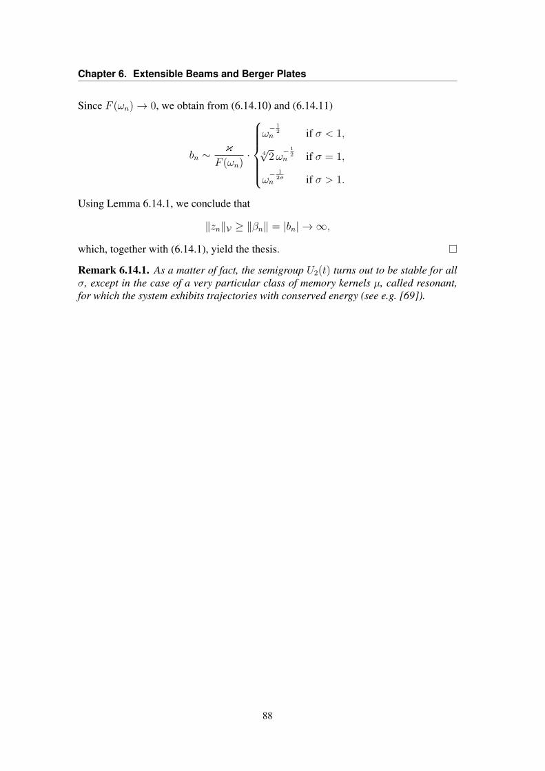
Chapter 6. Extensible Beams and Berger Plates
Since F (ωn) → 0, we obtain from (6.14.10) and (6.14.11)
bn ∼ κF (ωn)
·
ω− 1
2n if σ < 1,
4√2ω
− 12
n if σ = 1,
ω− 1
2σn if σ > 1.
Using Lemma 6.14.1, we conclude that
∥zn∥V ≥ ∥βn∥ = |bn| → ∞,
which, together with (6.14.1), yield the thesis.
Remark 6.14.1. As a matter of fact, the semigroup U2(t) turns out to be stable for allσ, except in the case of a very particular class of memory kernels µ, called resonant,for which the system exhibits trajectories with conserved energy (see e.g. [69]).
88

CHAPTER7
Caginalp Phase-Field Systems
7.1 Introduction
Let Ω ⊂ R3 be a bounded domain with smooth boundary ∂Ω. We consider the follow-ing nonlinear system of Caginalp type in the unknowns u = u(x, t) : Ω×R+ → R andα = α(x, t) : Ω× R+ → R
ut −∆u+ ϕ(u) = αt,
αtt −∆αt −∆α + g(α) = −ut,(7.1.1)
supplemented with the initial datau(x, 0) = u0(x),
α(x, 0) = α0(x),
αt(x, 0) = α1(x),
and Dirichlet boundary conditions,u(x, t)|x∈∂Ω = 0,
α(x, t)|x∈∂Ω = 0.
As detailed in the introduction of the thesis, system (7.1.1) serves as a model in thedescription of type III phase-field evolutions, with order parameter u and thermal dis-placement α.
89

Chapter 7. Caginalp Phase-Field Systems
Assumptions on the nonlinearities. We assume that ϕ, g ∈ F , where F is the class offunctions
F = f ∈ C1(R) : f(0) = 0 and |f ′(s)| ≤ c+c|s|4, for all s ∈ R and some c ≥ 0 .
Furthermore, we require the following dissipation conditions (in the sense that they al-low to prove the dissipativity of the associated semigroup, i.e., the existence of boundedabsorbing sets, see below):
lim inf|s|→+∞
ϕ(s)
s> −λ1, (7.1.2)
lim inf|s|→+∞
g′(s) > −λ1, (7.1.3)
where λ1 > 0 is the first eigenvalue of the linear operator −∆ on L2(Ω) with domainH2(Ω) ∩H1
0 (Ω). Finally, we assume that
ϕ′(s) ≥ −c, for every s ∈ R. (7.1.4)
Our aim in this chapter is to study the asymptotic behavior of the solution semi-group associated to (7.1.1). The first results concerning well-posedness and existenceof global attractors for this model have been obtained in [63] in the case g = 0, underthe growth restriction
|ϕ′(s)| ≤ c+ c|s|r, r = 2,
and with (7.1.2) replaced by the less general condition
ϕ(s)s ≥∫ s
0
ϕ(y)dy ≥ −c.
Here, we develop the analysis under assumption (7.1.2), in the case of two nonlineari-ties ϕ and g, both of critical order r = 4, proving the existence of a global attractor ofoptimal regularity.
After introducing some preliminaries in Section 7.2, we prove the well-posedness inSection 7.3, yielding a solution semigroup (dynamical system) acting on the naturalweak energy space. In Sections 7.4-7.5, we turn to the study of the dissipativity ofthe semigroup, characterized by the existence of regular absorbing sets. The final Sec-tion 7.6 is devoted to the main result concerning existence and regularity of the globalattractor.
7.2 Preliminaries
7.2.1 Functional setting
Let A be the strictly positive Dirichlet operator
A = −∆ with domain D(A) = H2(Ω) ∩H10 (Ω) b L2(Ω).
Analogously to Chapter 2, for σ ∈ R we introduce the scale of (compactly) nestedHilbert spaces
Hσ = D(Aσ2 ),
90

7.2. Preliminaries
with inner product⟨w, v⟩σ = ⟨A
σ2w,A
σ2 v⟩
and norm∥w∥σ = ∥A
σ2w∥.
Again, for σ > 0, it is understood that H−σ denotes the completion of the domain, sothat H−σ is the dual space of Hσ. We omit the subscript σ whenever it equals zero andthe symbol ⟨·, ·⟩ also stands for the duality product between Hσ and H−σ. In particular,
H2 = H2(Ω) ∩H10 (Ω) b H1 = H1
0 (Ω) b H = L2(Ω) b H−1 = H−1(Ω).
We also define the energy spaces
Hσ = Hσ+1 × Hσ+1 × Hσ,
endowed with the standard product norms
∥w1, w2, w3∥2Hσ= ∥w1∥2σ+1 + ∥w2∥2σ+1 + ∥w3∥2σ.
7.2.2 Technical lemmas
We need the following Gronwall-type lemma.
Lemma 7.2.1. Let X be a Banach space and let Z ⊂ C(R+, X). Let E : X → R be afunction such that
inft∈R+
E(z(t)) ≥ −m, E(z(0)) ≤M,
for some m,M ≥ 0 and every z ∈ Z . In addition, assume that, for every z ∈ Z ,the function t 7→ E(z(t)) is continuously differentiable and satisfies the differentialinequality
d
dtE(z(t)) + µ∥z(t)∥2X ≤ k,
for some µ > 0 and k > 0, both independent of z ∈ Z . Then, there exists t0 = m+Mk
≥0 such that
E(z(t)) ≤ supζ∈X
E(ζ) : µ∥ζ∥2X ≤ 2k
, ∀t ≥ t0.
The proof can be found in [3]. We will also exploit the Uniform Gronwall Lemma(see, e.g., [91], Section 1.1.3) which reads as follows.
Lemma 7.2.2. Let Λ0 be an absolutely continuous nonnegative function and Λ1,Λ2
be two nonnegative functions satisfying, almost everywhere in R+, the differential in-equality
d
dtΛ0 ≤ Λ0Λ1 + Λ2.
Assume also that
supt≥0
∫ t+1
t
Λı(τ)dτ ≤ mı, ı = 0, 1, 2,
for some positive constants mı. Then, there exists c > 0 depending only on mi suchthat
Λ0(t+ 1) ≤ c, ∀t ≥ 0.
91

Chapter 7. Caginalp Phase-Field Systems
We finally recall a useful decomposition lemma stated in Chapter 2 (Lemma 2.3.1).
Lemma 7.2.3. Let g ∈ F satisfy (7.1.3). Then, for every λ < λ1 sufficiently close toλ1, the decomposition
g(s) = g0(s)− λs+ g1(s)
holds for some g0, g1 ∈ C1(R) with the following properties:
• g1 is compactly supported with g1(0) = 0;
• g0 vanishes inside [−1, 1] and fulfills, for some c ≥ 0 and every s ∈ R, the bounds
0 ≤ g′0(s) ≤ c|s|4.
Defining the following functionals on H1:
Φ(w) = 2
∫Ω
∫ w(x)
0
ϕ(y) dydx
and
G0(w) = 2
∫Ω
∫ w(x)
0
g0(y) dydx,
by (7.1.2) and Lemma 7.2.3, the inequalities
Φ(w) ≥ −(1− ν)∥w∥21 − c1, (7.2.1)
⟨ϕ(w), w⟩ ≥ −(1− ν)∥w∥21 − c1 (7.2.2)
and
0 ≤ G0(w) ≤ 2⟨g0(w), w⟩ (7.2.3)
hold for some 0 < ν < 1 and c1 ≥ 0.
Remark 7.2.1. Along the chapter, we will perform several formal estimates whichcan be justified within a proper Galerkin scheme. Moreover, the Holder, Young andPoincare inequalities will be used without explicit mention, as well as the Sobolev em-bedding
H1 ⊂ L6(Ω).
Remark 7.2.2. We stress that we study the model in the meaningful physical dimensionN = 3. Nonetheless, all the results are true in lower dimensions and can also beproved for N > 3: accordingly, one has to assume the correct critical growth on thenonlinearities ϕ′ and g′ (namely, 4
N−2instead of 4) and to exploit the corresponding
Sobolev embeddings.
92
7.3. The Solution Semigroup
7.3 The Solution Semigroup
We start by giving a suitable notion of weak solution.
Definition 7.3.1. Given T > 0, we call weak solution to (7.1.1) on [0, T ] a pair (u, α),
u ∈ C([0, T ],H1) ∩ C1([0, T ],H−1),
α ∈ C([0, T ],H1) ∩ C1([0, T ],H) ∩ C2([0, T ],H−1) ∩W 1,2(0, T ; H1),
satisfying, for almost every t ∈ [0, T ] and every test function (v, θ) ∈ H1 × H1, theequalities
⟨ut, v⟩+ ⟨u, v⟩1 + ⟨ϕ(u), v⟩ = ⟨αt, v⟩,⟨αtt, θ⟩+ ⟨αt, θ⟩1 + ⟨α, θ⟩1 + ⟨g(α), θ⟩ = −⟨ut, θ⟩.
Theorem 7.3.1. For every T > 0 and every z0 = a1, a2, a3 ∈ H, system (7.1.1)admits a unique weak solution (u, α) on [0, T ] such that
u(0), α(0), αt(0) = z0.
In addition, given R > 0, for any pair of initial data z1, z2 ∈ H such that ∥z1∥H ≤ Rand ∥z2∥H ≤ R, the difference (u, α) = (u1 − u2, α1 − α2) of the correspondingsolutions satisfies
∥u, α, αt∥L∞(0,T ;H) ≤ KeKT∥z1 − z2∥H, (7.3.1)
for some constant K = K(R) ≥ 0.
Proof. Concerning existence, this follows from a usual Galerkin procedure, consider-ing the solutions (un, αn) to n-dimensional approximating problems. Arguing as in theforthcoming Theorem 7.4.1 and Corollary 7.4.1, with (un, αn) in place of (u, α), wededuce the boundedness of
un in L∞(0, T ; H1) ∩ L2(0, T ; H2),
∂tun in L2(0, T ; H),
αn in L∞(0, T ; H1),
∂tαn in L∞(0, T ; H) ∩ L2(0, T ; H1),
and, calling ΩT = Ω × (0, T ), those of ϕ(un) and g(αn) in L65 (ΩT ). Hence, we can
extract (weakly or weakly-∗) convergent subsequences to some limit (u, α). Provingthat this limit solves the original problem is a standard matter, as well as the proof ofthe regularity
u ∈ C([0, T ],H1).
Moreover, arguing as in Chapter 2 (proof of Theorem 2.4.1), we obtain
α ∈ C([0, T ],H1) ∩ C1([0, T ],H).
93
Chapter 7. Caginalp Phase-Field Systems
The required regularity in H−1 of both u and α is now immediately seen by comparisonin the equations. It remains to prove (7.3.1). Setting u = u1 − u2 and α = α1 −α2, thedifference system reads
ut −∆u+ ϕ(u1)− ϕ(u2) = αt,
αtt −∆αt −∆α + g(α1)− g(α2) = −ut.
Along the proof, the generic constant K ≥ 0 may depend on R. Multiplying the firstequation by 2ut, the second one by 2αt and summing up, we obtain
d
dtΛ + 2∥ut∥2 + 2∥αt∥21 = 2⟨ϕ(u2)− ϕ(u1), ut⟩+ 2⟨g(α2)− g(α1), αt⟩, (7.3.2)
whereΛ = ∥u∥21 + ∥α∥21 + ∥αt∥2.
The growth of g and Corollary 7.4.1 entail
2⟨g(α2)− g(α1), αt⟩ ≤ K∥α∥1∥αt∥1 ≤ ∥αt∥21 +K∥α∥21.
Using the embedding H5/4 ⊂ L12(Ω), we have
2⟨ϕ(u2)− ϕ(u1), ut⟩ ≤ K∥u∥1∥ut∥[1 + ∥u2∥45/4 + ∥u1∥45/4
].
Furthermore, a classical interpolation inequality yields
∥uı∥45/4 ≤ K∥uı∥31∥uı∥2. (7.3.3)
Thus, accounting for Corollary 7.4.1, the right-hand side of (7.3.2) is controlled by
∥ut∥2 + ∥αt∥21 +K[1 + ∥u2∥22 + ∥u1∥22
]Λ
and we end up withd
dtΛ ≤ K
[1 + ∥u2∥22 + ∥u1∥22
]Λ.
An application of the Gronwall lemma, along with Corollary 7.4.1, completes the proof.
In light of Theorem 7.3.1, system (7.1.1) generates a dynamical system S(t) on thephase space H, defined by
S(t)z0 = z(t) = u(t), α(t), αt(t),
where (u(t), α(t)) is the solution at time twith initial datum z0 = u(0), α(0), αt(0) ∈H.
94

7.4. A Priori Estimates and Dissipativity
7.4 A Priori Estimates and Dissipativity
As already said, the presence of some dissipation mechanism in the dynamical systemS(t) reflects into the existence of an absorbing set.
Theorem 7.4.1. There exists a constant R0 > 0 with the following property: given anyR ≥ 0, there exists te = te(R) ≥ 0 such that, whenever
∥z0∥H ≤ R,
the inequality∥S(t)z0∥H ≤ R0
holds for every t ≥ te.
In order to simplify the calculations, according to Lemma 7.2.3, we fix λ sufficientlyclose to λ1 and rewrite the nonlinear Caginalp system (7.1.1) as
ut −∆u+ ϕ(u) = αt,
αtt −∆αt −∆α + g0(α)− λα = −ut − q,(7.4.1)
with q = g1(α). In addition, given any solution (u, α) to (7.4.1), we introduce theequivalent inner product (·, ·)1 on H1 defined by
(w, v)1 = ⟨w, v⟩1 − λ⟨w, v⟩,
with induced norm | · |1. The corresponding energy reads
E(t) = ∥u(t)∥21 + |α(t)|21 + ∥αt(t)∥2.
Proof of Theorem 7.4.1. Let C ≥ 0 be a generic constant independent of R and setS(t)z0 = z(t). Due to (7.2.1)-(7.2.3) and the growth of ϕ and g0, the functional
E(z(t)) =∥u(t)∥21 + ε∥u(t)∥2 + ∥αt(t)∥2 + |α(t)|21+ε∥α(t)∥21 + 2ε⟨αt(t), α(t)⟩+ Φ(u(t)) +G0(α(t))
fulfills, for ε > 0 small,E(z(t)) ≥ νE(t)− C (7.4.2)
andE(z(t)) ≤ CE(t)
[1 + E(t)2
]. (7.4.3)
Multiplying the first equation of (7.4.1) by 2ut+2εu, the second one by 2αt+2εα andsumming up, we infer
d
dtE+2∥ut∥2 + 2ε∥u∥21 + 2∥αt∥21 − 2ε∥αt∥2
+2ε|α|21 + 2ε⟨ϕ(u), u⟩+ 2ε⟨g0(α), α⟩
=2ε⟨αt, u⟩ − 2ε⟨ut, α⟩ − ⟨q, 2αt + 2εα⟩.
95

Chapter 7. Caginalp Phase-Field Systems
Thus, by (7.2.2) and (7.2.3),
d
dtE+∥ut∥2 +
3
2∥αt∥21 + 2εν∥u∥21 + 2ε|α|21
≤2ε⟨αt, u⟩ − 2ε⟨ut, α⟩ − ⟨q, 2αt + 2εα⟩+ 2εc1,
for ε > 0 small enough. Possibly reducing ε, we have
−⟨q, 2αt + 2εα⟩ ≤ 1
4∥αt∥21 +
ε
4|α|21 + C
and2ε⟨αt, u⟩ − 2ε⟨ut, α⟩ ≤
1
2∥ut∥2 +
1
4∥αt∥21 + εν∥u∥21 +
ε
4|α|21.
Therefore,
d
dtE + µ
[∥u∥21 + ∥α∥21 + ∥αt∥2
]+
1
2∥ut∥2 +
1
2∥αt∥21 ≤ C,
for some µ > 0, andd
dtE(z(t)) + µ∥z(t)∥2H ≤ C.
Applying Lemma 7.2.1, together with (7.4.2) and (7.4.3), we finish the proof of thetheorem.
Corollary 7.4.1. Given any R ≥ 0, there exists a constant K = K(R) ≥ 0 such that,whenever ∥z0∥ ≤ R, the corresponding solution S(t)z0 fulfills
∥S(t)z0∥H ≤ K, ∀t ≥ 0, (7.4.4)
and ∫ T
t
[∥ut(τ)∥2 + ∥αt(τ)∥21 + ∥u(τ)∥22
]dτ ≤ K +K(T − t), ∀ T > t ≥ 0.
Proof. Along the proof, K ≥ 0 denotes a generic constant depending on R. Recastingword by word the proof of Theorem 7.4.1 with ε = 0, we end up with
d
dt
[∥u∥21 + ∥αt∥2 + |α|21 + Φ(u) +G0(α)
]+ ∥ut∥2 + ∥αt∥21 ≤ C, (7.4.5)
for some C ≥ 0 (independent of R). Fix any t ≤ te(R) and integrate the last inequalityover [0, t] to find, in light of (7.2.1)-(7.2.3),
E(t) ≤ K.
Applying Theorem 7.4.1, we conclude that ∥S(t)z0∥H ≤ K for every t ≥ 0. Toprove the remaining bounds, we integrate inequality (7.4.5) over [t, T ] and obtain therequired estimates for ut in L2(t, T ; H) and αt in L2(t, T ; H1). The product in H of thefirst equation of (7.4.1) by −2∆u reads
d
dt∥u∥21 + 2∥u∥22 + 2⟨ϕ′(u)∇u,∇u⟩ = −2⟨αt,∆u⟩.
96

7.5. Further Dissipativity
Using (7.1.4) and (7.4.4), we end up with
d
dt∥u∥21 + ∥u∥22 ≤ K
and, integrating over [t, T ], the claim is proved.
According to (7.4.4), the set
B0 = z0 ∈ H : ∥S(t)z0∥H ≤ K(R0), ∀t ≥ 0
is an invariant absorbing set for the semigroup S(t).
Remark 7.4.1. It is worth noticing that the bound from below on ϕ′, assumed in (7.1.4),is not needed for the existence of the absorbing set B0.
Remark 7.4.2. All the results obtained in this section are a priori estimates and do notmake use of Theorem 7.3.1.
7.5 Further Dissipativity
A deeper analysis of the dissipation mechanism involved in the system allows to dis-cover a partial regularization effect on the solutions.
Theorem 7.5.1. There exists an invariant absorbing set B such that
supt≥0
supz0∈B
[∥u(t)∥2 + ∥ut(t)∥1 + ∥αt(t)∥1 + ∥αtt(t)∥
]< +∞.
The proof of Theorem 7.5.1 can be divided into two steps. First, we obtain the regu-larization of u and αt.
Lemma 7.5.1. There exists an invariant absorbing set B1 such that
supt≥0
supz0∈B1
[∥u(t)∥2 + ∥αt(t)∥1
]< +∞.
Proof. In what follows, C ≥ 0 denotes a generic constant depending only on the in-variant absorbing set B0 constructed in the previous section. Consider an initial datumz0 ∈ B0. Owing to (7.1.4) and the growth of g0, the functional
Λ = Λ(S(t)z0) = ∥u∥22 + ∥u∥21 + ∥αt∥21 + 2(α, αt)1 + 2⟨g0(α), αt⟩+K0
satisfies, for K0 = K0(B0) > 0 sufficiently large,
∥u∥22 + ∥αt∥21 ≤ 2Λ ≤ C[1 + ∥u∥22 + ∥αt∥21
]. (7.5.1)
Multiplying the first equation of (7.4.1) by −2∆(ut + u), the second one by 2αtt andsumming up, we find
d
dtΛ + 2∥u∥22 + 2∥ut∥21 + 2∥αtt∥2 + 2⟨ϕ′(u)∇u,∇u⟩
= 2|αt|21 − 2⟨ϕ′(u)∇u,∇ut⟩+ 2⟨g′0(α)αt, αt⟩
− 2⟨αt,∆ut⟩ − 2⟨αt,∆u⟩ − 2⟨ut, αtt⟩ − 2⟨q, αtt⟩.
97

Chapter 7. Caginalp Phase-Field Systems
By (7.1.4), we have2⟨ϕ′(u)∇u,∇u⟩ ≥ −C,
while, by the growth assumption on ϕ and g0, exploiting the embedding H5/4 ⊂ L12(Ω)and interpolation (see inequality (7.3.3)),
−2⟨ϕ′(u)∇u,∇ut⟩ ≤ C∥ut∥1∥u∥2[1 + ∥u∥45/4
]≤ ∥ut∥21 + C
[1 + ∥u∥22
]Λ
and2⟨g′0(α)αt, αt⟩ ≤ C∥αt∥21 ≤ CΛ.
Next, noting that
−2⟨ut, αtt⟩ − 2⟨q, αtt⟩ ≤ C[1 + ∥ut∥2
]+ ∥αtt∥2
and2|αt|21 − 2⟨αt,∆ut⟩ − 2⟨αt,∆u⟩ ≤ CΛ +
1
2∥u∥22 +
1
2∥ut∥21 + C,
we end up with
d
dtΛ +
1
2∥ut∥21 +
1
2∥αtt∥2 ≤ C
[1 + ∥u∥22
]Λ + C
[1 + ∥ut∥2
]. (7.5.2)
Hence, setting
Λ0(t) =t
t+ 1Λ(S(t)z0),
elementary computations provide
d
dtΛ0(t) ≤ h(t)Λ0(t) + k(t),
withh(t) = C
[1 + ∥u(t)∥22
]and
k(t) =1
[t+ 1]2Λ(S(t)z0) + C
[t
t+ 1
[1 + ∥ut(t)∥2
]].
Since, by Corollary 7.4.1 and (7.5.1), there holds
supt≥0
∫ t+1
t
[Λ0(τ) + h(τ) + k(τ)
]dτ ≤ C,
applying Lemma 7.2.2, we have
Λ0(t+ 1) ≤ C, ∀t ≥ 0,
and, in particular,Λ(S(1)z0) ≤ C.
The setB1 = S(1)B0 ⊂ B0,
98

7.5. Further Dissipativity
is clearly absorbing and invariant. Moreover,
supt≥0
supz0∈B1
Λ(S(t)z0) = supt≥0
supz0∈B0
Λ(S(t+ 1)z0) ≤ supz0∈B0
Λ(S(1)z0) ≤ C,
which, along with (7.5.1), establishes the desired bound
supt≥0
supz0∈B1
[∥u(t)∥2 + ∥αt(t)∥1
]≤ C.
Corollary 7.5.1. We have the uniform estimate
supt≥0
supz0∈B1
[∥ut(t)∥+
∫ t+1
t
[∥ut(τ)∥21 + ∥αtt(τ)∥2
]dτ
]< +∞.
Proof. The control of ut in L∞(R+; H) immediately follows by comparison in the firstequation of (7.4.1). Integrating (7.5.2) over [t, t+ 1], we finish the proof.
Proof of Theorem 7.5.1. Take an initial datum z0 ∈ B1 and consider a generic constantC ≥ 0 depending only on B1. Differentiating system (7.4.1) with respect to time, weobtain
utt −∆ut + ϕ′(u)ut = αtt,
αttt −∆αtt −∆αt + g′0(α)αt − λαt = −utt − qt.
Multiplying the first equation by 2utt, the second one by 2αtt and summing up, we find
d
dtΛ + 2∥utt∥2 + 2∥αtt∥21 = −2⟨ϕ′(u)ut, utt⟩ − 2⟨g′0(α)αt, αtt⟩ − 2⟨qt, αtt⟩,
whereΛ = Λ(S(t)z0) = ∥ut∥21 + ∥αtt∥2 + |αt|21.
Due to the growth of ϕ and the Agmon inequality,
−2⟨ϕ′(u)ut, utt⟩ ≤ C∥utt∥ ≤ ∥utt∥2 + C,
while, using the growth of g0,
−2⟨g′0(α)αt, αtt⟩ − 2⟨qt, αtt⟩ ≤ C∥αtt∥1 ≤ ∥αtt∥21 + C.
Summarizing, we end up with
d
dtΛ + ∥utt∥2 + ∥αtt∥21 ≤ C.
At this point, multiplying both terms of the above inequality by t ∈ [0, 1], we have
d
dt
[tΛ(S(t)z0)
]≤ Λ(S(t)z0) + C.
By Lemma 7.5.1 and Corollary 7.5.1,∫ 1
0
Λ(S(t)z0) dt ≤ C,
99

Chapter 7. Caginalp Phase-Field Systems
hence, integrating over [0, 1],Λ(S(1)z0) ≤ C.
SettingB = S(1)B1 ⊂ B1,
which is absorbing and invariant, we conclude that
supt≥0
supz0∈B
Λ(S(t)z0) = supt≥0
supz0∈B1
Λ(S(t+ 1)z0) ≤ supz0∈B1
Λ(S(1)z0) ≤ C.
7.6 The Global Attractor
It follows from Theorem 7.5.1 that u(t) regularizes in finite time. Unfortunately, thiscannot occur for α(t), preventing the existence of a compact absorbing set for S(t).Nonetheless, it is still true that there exists a compact attracting set for the semigroup.More precisely, our main result is the existence of a compact set which is exponentiallyattracting in H for the semigroup.
Theorem 7.6.1. There exist three strictly positive constants ϱ, C1, ω1 and a closed ballBH1(ϱ) of H1 such that
δH(S(t)B,BH1(ϱ)) ≤ C1e−ω1t, t ≥ 0.
As a corollary we have existence of the global attractor A for S(t). Besides, since theglobal attractor is contained in any compact attracting set, it satisfies ∥A∥H1 ≤ ϱ.
Corollary 7.6.1. The semigroup S(t) : H → H possesses a (connected) global attrac-tor A which is bounded in H1.
In light of Theorem 7.5.1, which provides a regularization of u(t) in finite time, theproof of Theorem 7.6.1 is an immediate consequence of the following lemma.
Lemma 7.6.1. There exists a closed ball B in the space H2 × H1 such that
supz0∈B
δH1×H
(α(t), αt(t), B
)≤ C0e
−t, t ≥ 0, (7.6.1)
for some positive constant C0 depending only on B.
Proof. We exploit the “parabolic” approach developed in [73]. Accordingly, we takean initial datum z0 = a1, a2, a3 ∈ B and we write α = η + ζ , with
−∆ηt −∆η + g0(α)− g0(ζ) = 0,
η(0) = a2,
ηt(0) = a3,
(7.6.2)
and −∆ζt −∆ζ + g0(ζ) = h,
ζ(0) = 0,
ζt(0) = 0,
(7.6.3)
100

7.6. The Global Attractor
where, by force of Theorem 7.5.1,
h = λα− ut − q − αtt ∈ L∞(R+; H).
In what follows, the generic constant C ≥ 0 only depends on B. Multiplying (7.6.2) by2η, from the monotonicity of g0, we infer
d
dt∥η∥21 + 2∥η∥21 ≤ 0
and the Gronwall lemma entails
∥η(t)∥21 ≤ ∥η(0)∥21 e−2t, ∀t ≥ 0. (7.6.4)
Then, we multiply (7.6.3) by −2∆ζ . Using again the monotonicity of g0, we obtain
d
dt∥ζ∥22 + 2∥ζ∥22 ≤ −2⟨h,∆ζ⟩ ≤ C∥ζ∥2 ≤ C + ∥ζ∥22.
Thus,d
dt∥ζ∥22 + ∥ζ∥22 ≤ C
and the Gronwall lemma gives the uniform bound
∥ζ(t)∥22 ≤ C. (7.6.5)
Collecting (7.6.4), (7.6.5) and Theorem 7.5.1, we see that, for every initial datum z0 ∈B,
∥η(t)∥1 ≤ Ce−t, ∥ζ(t)∥2 ≤ C, ∥αt(t)∥1 ≤ C.
Hence, calling B the ball of H2 × H1 of radius C√2, we complete the proof.
Remark 7.6.1. The existence of a global attractor bounded in H1 for the semigroupS(t) can also be proved within the weaker dissipativity assumption
lim inf|s|→∞
g(s)
s> −λ1.
In that case, the proof of Theorem 7.6.1 is indeed more complicated and requires anabstract result from [21] (see Theorem A.4 in the appendix). We stress out that, con-trary to Lemma 7.6.1 in which the attraction property for α is obtained separately, thealternative technique needs a suitable splitting of the whole semigroup. The interestedreader can find the proper decomposition for α in [21, Section 4] (see also [72]) whichhas to be coupled with the “subcritical” splitting for u as in [21, Example 3.5].
Remark 7.6.2. In light of Theorem 7.5.1, the global attractor A is easily seen to bebounded in the more regular space H2 × H2 × H2.
101


CHAPTER8
Timoshenko Systems with Gurtin-PipkinThermal Law
8.1 Introduction
Given a real interval I = [0, ℓ], we consider the thermoelastic beam model of Timo-shenko type [92]
ρ1φtt − κ(φx + ψ)x = 0,
ρ2ψtt − bψxx + κ(φx + ψ) + δθx = 0,
ρ3θt + qx + δψtx = 0,
(8.1.1)
where the unknown variables
φ, ψ, θ, q : (x, t) ∈ I× [0,∞) 7→ R
represent the transverse displacement of a beam with reference configuration I, therotation angle of a filament, the relative temperature (i.e. the temperature variationfield from an equilibrium reference value) and the heat flux vector, respectively. Here,ρ1, ρ2, ρ3 as well as κ, b, δ are strictly positive fixed constants. The system is comple-mented with the Dirichlet boundary conditions for φ and θ
φ(0, t) = φ(ℓ, t) = θ(0, t) = θ(ℓ, t) = 0,
and the Neumann one for ψ
ψx(0, t) = ψx(ℓ, t) = 0.
103

Chapter 8. Timoshenko Systems with Gurtin-Pipkin Thermal Law
As already said in the introduction of the thesis, such boundary conditions seem to bethe most feasible from a physical viewpoint. To complete the picture, a further relationis needed: the so-called constitutive law for the heat flux, establishing a link between qand θ. This is what really characterizes the dynamics, since no mechanical dissipationis present in the system, and any possible loss of energy can be due only to thermaleffects.
8.1.1 The Fourier thermal law
A first choice is to assume the classical Fourier law of heat conduction
βq + θx = 0, (8.1.2)
where β > 0 is a fixed constant. In which case, the third equation of (8.1.1) becomes
ρ3θt −1
βθxx + δψtx = 0.
The exponential stability of the resulting Timoshenko-Fourier system has been ana-lyzed in [67]. There, the authors introduce the so-called stability number1
χ =ρ1κ
− ρ2b,
representing the difference of the inverses of the propagation speeds. The main resultof [67] reads as follows: the contraction semigroup generated by (8.1.1)-(8.1.2) actingon the triplet (φ, ψ, θ) is exponentially stable (in the natural weak energy space) if andonly if χ = 0.
8.1.2 The Cattaneo thermal law
As already said, the drawback of the Fourier law lies in the physical paradox of infinitepropagation speed of (thermal) signals, a typical side-effect of parabolicity. A differentmodel, removing this paradox, is the Cattaneo law [8], namely, the differential pertur-bation of (8.1.2)
τqt + βq + θx = 0, (8.1.3)
for τ > 0 small. A natural question is whether the semigroup generated by (8.1.1)coupled with (8.1.3), now acting on the state variable (φ, ψ, θ, q), remains exponentiallystable within the condition χ = 0 above. As shown in [31], the answer is negative:exponential stability can never occur when χ = 0. More recently, in [89] a new stabilitynumber is introduced in order to deal with the Timoshenko-Cattaneo system, that is,2
χτ =
[ρ1ρ3κ
− τ
][ρ1κ
− ρ2b
]− τ
ρ1δ2
ρ3κb.
1The notion of stability number is actually introduced in the subsequent paper [89], defined there as χ = κ/ρ1−b/ρ2. The difference is clearly irrelevant with respect to the relation χ = 0. The motivation of our choice of χ is torender more direct the comparison with the Cattaneo law.
2The value of χτ in [89] differs from ours for a multiplicative constant.
104

8.1. Introduction
The system is shown to be exponentially stable if and only if χτ = 0. Quite interest-ingly, the Fourier case is fully recovered in the limit τ → 0, when (8.1.3) collapsesinto (8.1.2). Indeed, for τ = 0 the equality
χ0 =ρ1ρ3κ
χ
holds, which tells at once that
χ0 = 0 ⇔ χ = 0.
It is worth mentioning that the proof of exponential stability in [89] is carried out vialinear semigroup techniques, whereas the analogous result of [67] for the Fourier caseis obtained by constructing explicit energy functionals.
8.1.3 The Gurtin-Pipkin thermal law
The aim of the present chapter is studying the Timoshenko system (8.1.1) assuming theGurtin-Pipkin heat conduction law for the heat flux [48]. More precisely, we considerthe constitutive equation
βq(t) +
∫ ∞
0
g(s)θx(t− s) ds = 0, (8.1.4)
where g, called the memory kernel, is a (bounded) convex summable function on [0,∞)of total mass ∫ ∞
0
g(s) ds = 1,
whose properties will be specified in more detail later on. Equation (8.1.4) can beviewed as a memory relaxation of the Fourier law (8.1.2), inducing (similarly to theCattaneo law) a fully hyperbolic mechanism of heat transfer. In this perspective, itmay be considered a more realistic description of physical reality. Accordingly, system(8.1.1) turns into
ρ1φtt − κ(φx + ψ)x = 0,
ρ2ψtt − bψxx + κ(φx + ψ) + δθx = 0,
ρ3θt −1
β
∫ ∞
0
g(s)θxx(t− s) ds+ δψtx = 0.
(8.1.5)
Rephrasing system (8.1.5) within the history framework of Dafermos [25], we con-struct a contraction semigroup S(t) of solutions acting on a suitable Hilbert space H,accounting for the presence of the memory. Then, introducing the stability number
χg =
[ρ1ρ3κ
− β
g(0)
][ρ1κ
− ρ2b
]− β
g(0)
ρ1δ2
ρ3κb,
our main theorem can be stated as follows.
Theorem 8.1.1. The semigroup S(t) is exponentially stable if and only if χg = 0.
105

Chapter 8. Timoshenko Systems with Gurtin-Pipkin Thermal Law
As we will see in the next section, Theorem 8.1.1 actually subsumes and generalizesall the previously known results on the exponential decay properties of the thermoelas-tic Timoshenko system (8.1.1).
Remark 8.1.1. Actually, exploiting the techniques of [10, 11], it is possible to provethat the contraction semigroup S(t) remains stable3 on H (although not exponentiallystable) also when χg = 0.
In Section 8.2 we compare Timoshenko systems of the form (8.1.1) subject to dif-ferent laws of heat conduction, viewed as particular instances of (8.1.5) for suitablechoices of the memory kernel. The comparison with the Timoshenko-Cattaneo systemof [31,89], only formal at this stage, is rendered rigorous in the final Section 8.8. Afterintroducing some notation (Section 8.3), in Section 8.4 we define the semigroup S(t)describing the solutions to (8.1.5). The subsequent three sections are devoted to theproof of Theorem 8.1.1. Firstly, we introduce some auxiliary functionals (Section 8.5),needed in the proof of the sufficiency part of the theorem carried out in Section 8.6. Thenecessity of the condition χg = 0 in order for exponential stability to occur is provedin Section 8.7.
8.2 Comparison with Earlier Results
8.2.1 The Fourier case
The Fourier law (8.1.2) can be seen as a (singular) limit of the Gurtin-Pipkin law (8.1.4).Indeed, defining the ε-scaling of the memory kernel g by
gε(s) =1
εg(sε
), ε > 0,
we consider in place of the original (8.1.4) the constitutive equation
βq(t) +
∫ ∞
0
gε(s)θx(t− s) ds = 0. (8.2.1)
Since gε → δ0 in the distributional sense, where δ0 denotes the Dirac mass at 0+, itis clear that, in the limit ε → 0, equation (8.2.1) reduces to the classical constitutivelaw (8.1.2). According to Theorem 8.1.1, exponential stability for the Timoshenko-Gurtin-Pipkin model with memory kernel gε occurs if and only if
χgε =
[ρ1ρ3κ
− βε
g(0)
][ρ1κ
− ρ2b
]− βε
g(0)
ρ1δ2
ρ3κb= 0.
Letting ε→ 0, we recover the condition
χδ0 =ρ1ρ3κ
χ = 0
of the Fourier case. The convergence of the Timoshenko-Gurtin-Pipkin model to theTimoshenko-Fourier one as ε → 0 can be made rigorous within the proper functionalsetting, along the same lines of [22].
3We recall that S(t) is said to be stable on H if
limt→∞
∥S(t)z∥H = 0, ∀z ∈ H.
106
8.2. Comparison with Earlier Results
8.2.2 The Cattaneo case
The Cattaneo law (8.1.3) can be deduced as a particular instance of (8.1.4), correspond-ing to the memory kernel
gτ (s) =β
τe−
sβτ .
Indeed, changing the integration variable, we can write the flux vector q in the form
q(t) = − 1
β
∫ t
−∞gτ (t− s)θx(s) ds.
Since
g′τ (s) = −βτgτ (s),
we draw the relation
qt(t) = − 1
β
∫ t
−∞g′τ (t− s)θx(s) ds−
gτ (0)
βθx(t) =
1
τ
∫ t
−∞gτ (t− s)θx(s) ds−
1
τθx(t),
which is nothing but (8.1.3). Besides, we have the equality of the stability numbers
χgτ = χτ .
8.2.3 The Coleman-Gurtin case
A further interesting model, midway between the Fourier and the Gurtin-Pipkin one, isobtained by assuming the (parabolic-hyperbolic) Coleman-Gurtin law for the heat flux,namely,
βq(t) + (1− α)θx(t) + α
∫ ∞
0
g(s)θx(t− s) ds = 0, α ∈ (0, 1). (8.2.2)
The limit cases α = 0 and α = 1 correspond to the fully parabolic Fourier case and thefully hyperbolic Gurtin-Pipkin case. The corresponding Timoshenko-Coleman-Gurtinsystem, whose third equation now reads
ρ3θt −1
β
[(1− α)θxx + α
∫ ∞
0
g(s)θxx(t− s) ds
]+ δψtx = 0,
generates (similarly to the Timoshenko-Gurtin-Pipkin system) a contraction semigroupΣ(t) on H. For this system, the following theorem holds.
Theorem 8.2.1. The semigroup Σ(t) is exponentially stable if and only if χ = 0.
Hence, the picture is exactly the same as in the Fourier case. This, as observed in [89],is due to the predominant character of parabolicity. Theorem 8.2.1 can be given adirect proof, following the lines of the next sections. In fact, the situation here is muchsimpler, do to the presence of instantaneous dissipation given by the term −θxx inthe equation. However, it is also possible to obtain Theorem 8.2.1 as a byproduct of
107

Chapter 8. Timoshenko Systems with Gurtin-Pipkin Thermal Law
Theorem 8.1.1. To this end, it is enough to consider the Timoshenko-Gurtin-Pipkinsystem with kernel
gε(s) =1− α
εg(sε
)+ αg(s),
whose exponential stability takes place if and only if
χgε =
[ρ1ρ3κ
− βε
(1− α + αε)g(0)
][ρ1κ
− ρ2b
]− βε
(1− α + αε)g(0)
ρ1δ2
ρ3κb= 0.
Performing the limit ε→ 0, we obtain the distributional convergence
gε → (1− α)δ0 + αg,
yielding in turn∫ ∞
0
gε(s)θxx(t− s) ds→ (1− α)θxx + α
∫ ∞
0
g(s)θxx(t− s) ds.
Accordingly, we see that
χ(1−α)δ0+αg =ρ1ρ3κ
χ,
and we recover the same stability condition of the Timoshenko-Fourier system.
8.2.4 Heat conduction of type III
We finally mention the model resulting from the constitutive law of type III of Green-Naghdi for the heat flux
βq + θx + dpx = 0, d > 0, (8.2.3)
where
p(t) = p(0) +
∫ t
0
θ(r) dr
is the thermal displacement. Plugging (8.2.3) into (8.1.1), one obtainsρ1φtt − κ(φx + ψ)x = 0,
ρ2ψtt − bψxx + κ(φx + ψ) + δptx = 0,
ρ3ptt − 1βptxx − d
βpxx + δψtx = 0.
In [61], the system is shown to be exponentially stable if χ = 0. Again, the partialparabolicity of the model prevails, so that the exponential stability condition is thesame as in the Fourier case. Though, the constitutive law (8.2.3) cannot be deducedfrom (8.1.4), not even as a limiting case. Possibly, this feature may reflect the fact thatthe theory of heat conduction of type III seems to be at the limit of thermodynamicadmissibility (see the analysis of [36]).
108

8.3. Functional Setting and Notation
8.3 Functional Setting and Notation
8.3.1 Assumptions on the memory kernel
Callingµ(s) = −g′(s),
the prime denoting the derivative with respect to s, let the following conditions hold.
(i) µ is a nonnegative nonincreasing absolutely continuous function on R+ such that
µ(0) = lims→0
µ(s) ∈ (0,∞).
(ii) There exists ν > 0 such that the differential inequality
µ′(s) + νµ(s) ≤ 0
holds for almost every s > 0.
Remark 8.3.1. For every k > 0, the exponential kernel g(s) = ke−ks meets the hy-potheses (i)-(ii).
In particular, µ is summable on R+ with∫ ∞
0
µ(s) ds = g(0).
Besides, the requirement that g has total mass 1 translates into∫ ∞
0
sµ(s) ds = 1.
8.3.2 Functional spaces
In what follows, ⟨·, ·⟩ and ∥ · ∥ are the standard inner product and norm on the Hilbertspace L2(I). We introduce the Hilbert subspace
L2∗(I) =
f ∈ L2(I) :
∫ ℓ
0
f(x) dx = 0
of zero-mean functions, along with the Hilbert spaces
H10 (I) and H1
∗ (I) = H1(I) ∩ L2∗(I),
both endowed with the gradient norm, due to the Poincare inequality. We also considerthe space H2(I) and so-called memory space
M = L2(R+;H10 (I))
of square summable H10 -valued functions on R+ with respect to the measure µ(s)ds,
endowed with the inner product
⟨η, ξ⟩M =
∫ ∞
0
µ(s)⟨ηx(s), ξx(s)⟩ ds.
109

Chapter 8. Timoshenko Systems with Gurtin-Pipkin Thermal Law
The infinitesimal generator of the right-translation semigroup on M is the linear oper-ator
Tη = −Dηwith domain
D(T ) =η ∈ M : Dη ∈ M, lim
s→0∥ηx(s)∥ = 0
,
where D stands for weak derivative with respect to the internal variable s ∈ R+. Thephase space of our problem will be
H = H10 (I)× L2(I)×H1
∗ (I)× L2∗(I)× L2(I)×M
normed by
∥(φ, φ, ψ, ψ, θ, η)∥2H = κ∥φx+ψ∥2+ρ1∥φ∥2+ b∥ψx∥2+ρ2∥ψ∥2+ρ3∥θ∥2+1
β∥η∥2M.
8.3.3 Basic facts on the memory space
For every η ∈ D(T ), the nonnegative functional
Γ[η] = −∫ ∞
0
µ′(s)∥ηx(s)∥2 ds
is well defined, and the following identity holds (see [11, 41, 69])
2⟨Tη, η⟩M = −Γ[η]. (8.3.1)
Moreover, in light of assumption (ii) on µ, we deduce the inequality
ν∥η∥2M ≤ Γ[η], (8.3.2)
which will be crucial for our purposes.
8.4 The Contraction Semigroup
Firstly, we introduce the auxiliary variable
η = ηt(x, s) : (x, t, s) ∈ I× [0,∞)× R+ 7→ R,
accounting for the integrated past history of θ and formally defined as (see [25, 41])
ηt(x, s) =
∫ s
0
θ(x, t− σ) dσ,
thus satisfying the Dirichlet boundary condition
ηt(0, s) = ηt(ℓ, s) = 0
and the further “boundary condition”
lims→0
ηt(x, s) = 0.
110
8.4. The Contraction Semigroup
Hence, η satisfies the equation
ηtt = −ηts + θ(t).
The way to render the argument rigorous is recasting (8.1.5) in the history space frame-work devised by C.M. Dafermos [25]. This amounts to considering the partial differ-ential system in the unknowns φ = φ(t), ψ = ψ(t), θ = θ(t) and η = ηt
ρ1φtt − κ(φx + ψ)x = 0, (8.4.1)
ρ2ψtt − bψxx + κ(φx + ψ) + δθx = 0, (8.4.2)
ρ3θt −1
β
∫ ∞
0
µ(s)ηxx(s) ds+ δψtx = 0, (8.4.3)
ηt = Tη + θ. (8.4.4)
Remark 8.4.1. The analogy with the original system (8.1.5) is not merely formal, andcan be made rigorous within the proper functional setting (see [41] for more details).
Introducing the state vector
z(t) = (φ(t), φ(t), ψ(t), ψ(t), θ(t), ηt),
we view (8.4.1)-(8.4.4) as the ODE in H
d
dtz(t) = Az(t), (8.4.5)
where the linear operator A is defined as
A
φ
φ
ψ
ψ
θ
η
=
φκρ1(φx + ψ)x
ψbρ2ψxx − κ
ρ2(φx + ψ)− δ
ρ2θx
1βρ3
∫∞0µ(s)ηxx(s) ds− δ
ρ3ψx
Tη + θ
with domain
D(A) =
(φ, φ, ψ, ψ, θ, η) ∈ H
∣∣∣∣∣∣∣∣∣∣∣∣∣∣∣∣∣
φ ∈ H2(I)
φ ∈ H10 (I)
ψx ∈ H10 (I)
ψ ∈ H1∗ (I)
θ ∈ H10 (I)
η ∈ D(T )∫∞0µ(s)η(s) ds ∈ H2(I)
.
111

Chapter 8. Timoshenko Systems with Gurtin-Pipkin Thermal Law
Theorem 8.4.1. The operator A is the infinitesimal generator of a contraction semi-group
S(t) = etA : H → H.The proof of this fact is based on Lemma 1.2.1, and is omitted (however, the argument
is similar to the one of Theorem 6.12.2). Thus, for every initial datum
z0 = (φ0, φ0, ψ0, ψ0, θ0, η0) ∈ Hgiven at time t = 0, the unique solution at time t > 0 to (8.4.5) reads
z(t) = (φ(t), φt(t), ψ(t), ψt(t), θ(t), ηt) = S(t)z0.
Besides, ηt fulfills the explicit representation formula (see [41])
ηt(s) =
∫ s
0θ(t− σ) dσ s ≤ t,
η0(s− t) +∫ t
0θ(t− σ) dσ s > t.
Remark 8.4.2. As observed in [67], the choice of the spaces of zero-mean functionsfor the variable ψ and its derivative is consistent. Indeed, calling
Θ(t) =
∫ ℓ
0
ψ(x, t) dx
and integrating (8.4.2) on I we obtain the differential equation
ρ2Θ(t) + κΘ(t) = 0.
Hence, if Θ(0) = Θ(0) = 0 it follows that Θ(t) ≡ 0.
Remark 8.4.3. For the existence of the contraction semigroup S(t) the hypotheses(i)-(ii) on the kernel are overabundant. It is actually enough to require that µ be a(nonnull and nonnegative) nonincreasing absolutely continuous summable function onR+, possibly unbounded in a neighborhood of zero.
For any fixed initial datum z0 ∈ H, we define (twice) the energy as
E(t) = ∥S(t)z0∥2H.The natural multiplication of equation (8.4.5) by z(t) in the weak energy space, alongwith an exploitation of (8.3.1), provide the energy identity
d
dtE(t) = 2⟨Az(t), z(t)⟩H =
2
β⟨Tηt, ηt⟩M = − 1
βΓ[ηt], (8.4.6)
valid for all z0 ∈ D(A).As anticipated in the introduction, the main Theorem 8.1.1 of this chapter tells that
S(t) exp. stable ⇔ χg = 0.
The proof of the result is carried out in the next Sections 8.5-8.7.
Remark 8.4.4. We mention that an alternative approach is also possible. Namely, toset the problem in the so-called minimal state framework [29], rather than in the pasthistory one. In which case, the necessary and sufficient condition χg = 0 of exponentialdecay remains the same. In fact, one can show in general that the exponential decayin the history space (i.e. what proved here) implies the analogous decay in the minimalstate space (cf. [19, 29]).
112

8.5. Some Auxiliary Functionals
8.5 Some Auxiliary Functionals
In this section, we define some auxiliary functionals needed in the proof of the suffi-ciency part of Theorem 8.1.1. As customary, it is understood that we work with (reg-ular) solutions arising from initial data belonging to the domain of the operator A.Along the section, C ≥ 0 will denote a generic constant depending only on the struc-tural quantities of the problem. Besides, we will tacitly use several times the Holder,Young and Poincare inequalities. In particular we will exploit the inequality∫ ∞
0
µ(s)∥ηx(s)∥ ds ≤(∫ ∞
0
µ(s) ds
) 12(∫ ∞
0
µ(s)∥ηx(s)∥2 ds) 1
2
=√g(0) ∥η∥M.
8.5.1 The functional I
LetI(t) = − 2ρ3
g(0)
∫ ∞
0
µ(s)⟨θ(t), ηt(s)⟩ ds.
Lemma 8.5.1. For every εI > 0 small, I satisfies the differential inequality
d
dtI + ρ3∥θ∥2 + ∥η∥2M ≤ εI∥ψt∥2 +
cIεIΓ[η]
for some cI > 0 independent of εI .
Proof. In light of (8.4.3) and (8.4.4), we have the identity
d
dtI + 2ρ3∥θ∥2 + ∥η∥2M =− 2ρ3
g(0)
∫ ∞
0
µ(s)⟨Tη(s), θ⟩ ds
+2
g(0)β
∥∥∥∥ ∫ ∞
0
µ(s)ηx(s) ds
∥∥∥∥2
− 2δ
g(0)
∫ ∞
0
µ(s)⟨ηx(s), ψt⟩ ds+ ∥η∥2M.
Integrating by parts in s, we infer that (as shown in [41], the boundary terms vanish)
− 2ρ3g(0)
∫ ∞
0
µ(s)⟨Tη(s), θ⟩ ds = − 2ρ3g(0)
∫ ∞
0
µ′(s)⟨η(s), θ⟩ ds
≤ C∥θ∥√Γ[η]
≤ ρ3∥θ∥2 + CΓ[η].
Thus, exploiting the inequalities
2
g(0)β
∥∥∥∥ ∫ ∞
0
µ(s)ηx(s) ds
∥∥∥∥2
≤ C∥η∥2M
and− 2δ
g(0)
∫ ∞
0
µ(s)⟨ηx(s), ψt⟩ ds ≤ C∥ψt∥∥η∥M,
113

Chapter 8. Timoshenko Systems with Gurtin-Pipkin Thermal Law
appealing to (8.3.2) we obtain for every εI > 0 small the estimate
d
dtI + ρ3∥θ∥2 + ∥η∥2M ≤ C∥ψt∥Γ[η] + CΓ[η] ≤ εI∥ψt∥2 +
C
εIΓ[η],
where C is independent of εI .
8.5.2 The functional J
Defining the primitive4
Ψ(x, t) =
∫ x
0
ψ(y, t) dy,
let
J(t) = −2ρ2ρ3δ
⟨θ(t),Ψt(t)⟩.
Lemma 8.5.2. For every εJ > 0 small, J satisfies the differential inequality
d
dtJ + ρ2∥ψt∥2 ≤ εJ
[∥ψx∥2 + ∥φx + ψ∥2
]+cJεJ
[∥θ∥2 + Γ[η]
]for some cJ > 0 independent of εJ .
Proof. By means of (8.4.2) and (8.4.3), we get
d
dtJ + 2ρ2∥ψt∥2
=2ρ2βδ
∫ ∞
0
µ(s)⟨ηx(s), ψt⟩ ds−2ρ3b
δ⟨θ, ψx⟩+
2ρ3κ
δ⟨θ, φ+Ψ⟩+ 2ρ3∥θ∥2.
Estimating the terms in the right-hand side as (here we use again (8.3.2))
2ρ2βδ
∫ ∞
0
µ(s)⟨ηx(s), ψt⟩ ds ≤ C∥ψt∥∥η∥M ≤ ρ2∥ψt∥2 + CΓ[η]
and, for every εJ > 0 small,
− 2ρ3b
δ⟨θ, ψx⟩+
2ρ3κ
δ⟨θ, φ+Ψ⟩+ 2ρ3∥θ∥2
≤ C[∥ψx∥+ ∥φx + ψ∥
]∥θ∥+ C∥θ∥2
≤ εJ[∥ψx∥2 + ∥φx + ψ∥2
]+C
εJ∥θ∥2,
with C independent of εJ , the claim follows.
4In particular, Ψ ∈ H10 (I).
114
8.5. Some Auxiliary Functionals
8.5.3 The functional K
We introduce the number
γg = κ− g(0)ρ1βρ3
depending on the memory kernel g. It is readily seen that
χg = 0 ⇒ γg = 0.
Then, assuming χg = 0 and calling
K1(t) =ρ1b
κ⟨ψx(t), φt(t)⟩+ ρ2⟨ψt(t), φx(t) + ψ(t)⟩,
K2(t) =
∫ ∞
0
µ(s)⟨ηtx(s), φx(t) + ψ(t)⟩ ds,
K3(t) = −δρ1κ
⟨θ(t), φt(t)⟩,
we set
K(t) =2κ
γg
[γgκK1(t)−
ρ1δ
βρ3κK2(t) +K3(t)
].
Lemma 8.5.3. Suppose that χg = 0. Then K satisfies the differential inequality
d
dtK + κ∥φx + ψ∥2 ≤ cK
[∥ψt∥2 + Γ[η]
]for some cK > 0.
Proof. In light of (8.4.1) and (8.4.2), we obtain the identity
d
dtK1 + κ∥φx + ψ∥2 =
(ρ2 −
ρ1b
κ
)⟨ψt, φtx⟩+ ρ2∥ψt∥2 − δ⟨θx, φx + ψ⟩. (8.5.1)
By (8.4.4),
d
dtK2 = −
∫ ∞
0
µ(s)⟨Tη(s), (φx + ψ)x⟩ ds− g(0)⟨θ, (φx + ψ)x⟩
−∫ ∞
0
µ(s)⟨ηxx(s), φt⟩ ds+∫ ∞
0
µ(s)⟨ηx(s), ψt⟩ ds.
From (8.4.3) we learn that
−∫ ∞
0
µ(s)⟨ηxx(s), φt⟩ ds = −βρ3⟨θt, φt⟩+ βδ⟨ψt, φtx⟩,
while an integration by parts in s yields (again, the boundary terms vanish)
−∫ ∞
0
µ(s)⟨Tη(s), (φx + ψ)x⟩ ds =∫ ∞
0
µ′(s)⟨ηx(s), φx + ψ⟩ ds.
115

Chapter 8. Timoshenko Systems with Gurtin-Pipkin Thermal Law
We conclude thatd
dtK2 =
∫ ∞
0
µ′(s)⟨ηx(s), φx + ψ⟩ ds+∫ ∞
0
µ(s)⟨ηx(s), ψt⟩ ds (8.5.2)
− βρ3⟨θt, φt⟩+ βδ⟨ψt, φtx⟩+ g(0)⟨θx, φx + ψ⟩.Finally, exploiting once more (8.4.1),
d
dtK3 = −δρ1
κ⟨θt, φt⟩+ δ⟨θx, φx + ψ⟩. (8.5.3)
At this point, reconstructing K from (8.5.1)-(8.5.3), we are led to the differential iden-tity
d
dtK + 2κ∥φx + ψ∥2
= χg2g(0)κb
βγg⟨ψt, φtx⟩+ 2ρ2∥ψt∥2
− 2ρ1δ
βγgρ3
[ ∫ ∞
0
µ′(s)⟨ηx(s), φx + ψ⟩ ds+∫ ∞
0
µ(s)⟨ηx(s), ψt⟩ ds].
Since χg = 0 by assumption, we are left to control the integral terms in the right-handside. We have
− 2ρ1δ
βγgρ3
∫ ∞
0
µ′(s)⟨ηx(s), φx + ψ⟩ ds ≤ C∥φx + ψ∥∫ ∞
0
−µ′(s)∥ηx(s)∥ ds
≤ C∥φx + ψ∥√Γ[η]
≤ κ∥φx + ψ∥2 + CΓ[η],
and, recalling (8.3.2),
− 2ρ1δ
βγgρ3
∫ ∞
0
µ(s)⟨ηx(s), ψt⟩ ds ≤ C∥ψt∥∥η∥M ≤ C∥ψt∥2 + CΓ[η].
The proof is completed.
8.5.4 The functional L
LetL(t) = 2ρ2⟨ψt(t), ψ(t)⟩ − 2ρ1⟨φt(t), φ(t)⟩.
Lemma 8.5.4. The functional L satisfies the differential inequalityd
dtL+ ρ1∥φt∥2 + b∥ψx∥2 ≤ cL
[∥φx + ψ∥2 + ∥ψt∥2 + ∥θ∥2
]for some cL > 0.
Proof. By means of (8.4.1) and (8.4.2),d
dtL+2ρ1∥φt∥2 +2b∥ψx∥2 = 2ρ2∥ψt∥2 +2δ⟨θ, ψx⟩+2κ∥φx +ψ∥2 − 4κ⟨φx +ψ, ψ⟩.
Since the right-hand side is easily controlled by
b∥ψx∥2 + C[∥φx + ψ∥2 + ∥ψt∥2 + ∥θ∥2
],
we are done.
116

8.6. Proof of Theorem 8.1.1 (Sufficiency)
8.6 Proof of Theorem 8.1.1 (Sufficiency)
Within the condition χg = 0, we are now in the position to prove the exponentialstability of S(t). In what follows, E is (twice) the energy, whereas I, J,K, L denotethe functionals of the previous Section 8.5.
8.6.1 A further energy functional
For ε > 0, we define
Mε(t) = I(t) + εJ(t) +ερ22cK
K(t) + ε√εL(t),
where cK > 0 is the constant of Lemma 8.5.3.
Lemma 8.6.1. For every ε > 0 sufficiently small, the differential inequality
d
dtMε + ε2E ≤ cM
εΓ[η]
holds for some cM > 0 independent of ε.
Proof. Collecting the inequalities of Lemmas 8.5.1, 8.5.2, 8.5.3 and 8.5.4, we end upwith
d
dtMε + ε
(κρ22cK
− εJ −√ε cL
)∥φx + ψ∥2 + ε
√ε ρ1∥φt∥2 + ε(
√ε b− εJ)∥ψx∥2
+(ερ2
2− εI − ε
√ε cL
)∥ψt∥2 +
(ρ3 − ε
√ε cL − εcJ
εJ
)∥θ∥2 + ∥η∥2M
≤(cIεI
+εcJεJ
+ερ22
)Γ[η].
At this point, we choose
εI =ερ24
and εJ =2εcJρ3
.
Taking ε > 0 sufficiently small, the claim follows.
8.6.2 Conclusion of the proof of Theorem 8.1.1
By virtue of (8.4.6) and Lemma 8.6.1, for ε > 0 sufficiently small the functional
Gε(t) = E(t) + ε2Mε(t)
fulfills the differential inequality
d
dtGε + ε4E ≤ −
( 1
β− cMε
)Γ[η] ≤ 0.
It is also clear from the definition of the functionals involved that, for all ε > 0 small,
1
2E(t) ≤ Gε(t) ≤ 2E(t).
Therefore, an application of the Gronwall lemma entails the required exponential decayof the energy.
117

Chapter 8. Timoshenko Systems with Gurtin-Pipkin Thermal Law
Remark 8.6.1. It is worth observing that, contrary to what done in [89], here the proofof exponential stability is based on the construction of explicit energy-like functionals.The advantage (with respect to linear semigroups techniques) is that the same calcula-tions apply to the analysis of nonlinear version of the problem, allowing, for instance,to prove the existence of absorbing sets.
8.7 Proof of Theorem 8.1.1 (Necessity)
In this section, we prove that the semigroup S(t) is not exponentially stable when thestability number χg is different from zero. According to the abstract Lemma 1.2.2of Chapter 1, we show that condition (1.2.1) fails to hold assuming, without loss ofgenerality, ℓ = π. Accordingly, for every n ∈ N, the vector
ζn =(0, sinnx
ρ1, 0, 0, 0, 0
)satisfies
∥ζn∥H =√
π2ρ1
.
For all n ∈ N, we denote for short
λn =√
κρ1n
and we study the equationiλnzn − Azn = ζn
in the unknown variable
zn = (φn, φn, ψn, ψn, θn, ηn).
Our conclusion is reached if we show that zn is not bounded in H, since this wouldviolate (1.2.1). Straightforward calculations entail the system
ρ1λ2nφn + κ(φnx + ψn)x = − sinnx,
ρ2λ2nψn + bψnxx − κ(φnx + ψn)− δθnx = 0,
iρ3λnθn −1
β
∫ ∞
0
µ(s)ηnxx(s) ds+ iδλnψnx = 0,
iλnηn − Tηn − θn = 0.
We now look for solutions (compatible with the boundary conditions) of the form
φn = An sinnx,
ψn = Bn cosnx,
θn = Cn sinnx,
ηn = ϕn(s) sinnx,
118

8.7. Proof of Theorem 8.1.1 (Necessity)
for some An, Bn, Cn ∈ C and some complex square summable function ϕn on R+ withrespect to the measure µ(s)ds, satisfying ϕn(0) = 0. This yields
κnBn = 1,
knAn +(− ρ2λ
2n + bn2 + κ
)Bn + δnCn = 0,
iρ3λnCn +n2
β
∫ ∞
0
µ(s)ϕn(s) ds− iδλnnBn = 0,
iλnϕn + ϕ′n − Cn = 0.
An integration of the last equation gives
ϕn(s) =Cn
iλn
(1− e−iλns
).
Substituting the result into the third equation above, and denoting by
µ(λn) =
∫ ∞
0
µ(s)e−iλns ds
the Fourier transform5 of µ, we find the explicit solution
An =ρ2κn
2 − ρ1bn2 − ρ1κ
ρ1κ2n2− δ2β
ρ3κβγg + ρ1κµ(λn),
where, according to the notation of Section 8.5,
γg = κ− g(0)ρ1βρ3
.
At this point, we consider separately two cases.
Case γg = 0
We have
An =ρ2κn
2 − ρ1bn2 − ρ1κ
ρ1κ2n2− δ2β
ρ1κµ(λn).
Due to the convergence µ(λn) → 0, ensured by the Riemann-Lebesgue lemma, we findthe asymptotic expression as n→ ∞
An ∼ − δ2β
ρ1κµ(λn).
Since∥zn∥2H ≥ κ∥φnx + ψn∥2 + b∥ψnx∥2,
there exists ϖ > 0 such that
∥zn∥H ≥ ϖ∥φnx∥ = ϖn|An|(∫ π
0
cos2 nx dx
) 12
=ϖ√π√2n|An| → ∞.
5Since µ is continuous nonincreasing and summable, it is easy to see that µ(λn) = 0 for every n.
119

Chapter 8. Timoshenko Systems with Gurtin-Pipkin Thermal Law
Case γg = 0
Exploiting again the Riemann-Lebesgue lemma, we now get
An → 1
κ
(ρ2ρ1
− b
κ
)− δ2
ρ3κγg=ρ3bg(0)
ρ1ρ3βγgχg = 0,
as χg = 0 by assumption. As before, we end up with
∥zn∥H ≥ ϖ√π√2n|An| → ∞.
This finishes the proof.
Remark 8.7.1. The proof above actually holds within the same minimal assumptionson the memory kernel ensuring the existence of S(t), i.e. µ nonnull, nonnegative, non-increasing, absolutely continuous and summable on R+.
8.8 More on the Comparison with the Cattaneo Model
As previously observed in Section 8.2, at a formal level it is possible to recover theexponential stability (as well as the lack of exponential stability) of the Timoshenko-Cattaneo system from our main Theorem 8.1.1. Here, we give a rigorous proof of thisfact. To this aim, let us write explicitly the system studied in [31, 89]
ρ1φtt − κ(φx + ψ)x = 0,
ρ2ψtt − bψxx + κ(φx + ψ) + δθx = 0,
ρ3θt + qx + δψtx = 0,
τqt + βq + θx = 0,
which generates a contraction semigroup S(t) acting on the phase space
H = H10 (I)× L2(I)×H1
∗ (I)× L2∗(I)× L2(I)× L2(I)
normed by
∥(φ, φ, ψ, ψ, θ, q)∥2H = κ∥φx + ψ∥2 + ρ1∥φ∥2 + b∥ψx∥2 + ρ2∥ψ∥2 + ρ3∥θ∥2 + τ∥q∥2.
According to the article [89], the semigroup S(t) is exponentially stable if and only ifthe stability number χτ equals zero.
Along with S(t), we consider the semigroup S(t) on H generated by (8.4.5) for theparticular choice of the kernel
µ(s) = −g′τ (s) =β2
τ 2e−
sβτ .
Then, we define the map Λ : M → L2(I) as
Λη = − 1
β
∫ ∞
0
µ(s)ηx(s) ds.
120
8.8. More on the Comparison with the Cattaneo Model
On account of the Holder inequality,
τ∥Λη∥2 ≤ τ
β2
[ ∫ ∞
0
µ(s)∥ηx(s)∥ ds]2
≤ 1
β∥η∥2M. (8.8.1)
Due to the peculiar form of the kernel, the following result is a direct consequence ofthe equations. The easy proof is left to the reader.
Lemma 8.8.1. Let z0 = (u0, η0) ∈ H be any initial datum, where u0 subsumes the first5 components of z0, and call z0 = (u0,Λη0) ∈ H. Then the first 5 components of S(t)z0and S(t)z0 coincide. Besides, the last component q(t) of S(t)z0 fulfills the equality
q(t) = Ληt,
where ηt is the last component of S(t)z0.
The full equivalence between the two models is established in the next two proposi-tions.
Proposition 8.8.1. If S(t) is exponentially stable on H, then so is S(t) on H.
Proof. Let z0 = (u0, q0) ∈ H be fixed. Choosing η0 ∈ M of the form
η0(x, s) = −τ∫ x
0
q0(y) dy,
it is readily seen that Λη0 = q0 and
1
β∥η0∥2M =
τ 2
β∥q0∥2
∫ ∞
0
µ(s) ds = τ∥q0∥2.
Lemma 8.8.1 yields the identity
∥S(t)z0∥H = ∥S(t)(u0,Λη0)∥H = ∥(u(t),Ληt)∥H,
where u(t) denotes the first 5 components of either solution. On the other hand, weinfer from (8.8.1) and the exponential stability of S(t) that
∥(u(t),Ληt)∥H ≤ ∥(u(t), ηt)∥H ≤ C∥(u0, η0)∥He−ωt,
for some ω > 0 and C ≥ 1. Since
∥(u0, η0)∥H = ∥z0∥H,
we are finished.
Proposition 8.8.2. If S(t) is exponentially stable on H, then so is S(t) on H.
Proof. To simplify the notation, we introduce the 5-component space
V = H10 (I)× L2(I)×H1
∗ (I)× L2∗(I)× L2(I)
121

Chapter 8. Timoshenko Systems with Gurtin-Pipkin Thermal Law
normed by
∥(φ, φ, ψ, ψ, θ)∥2V = κ∥φx + ψ∥2 + ρ1∥φ∥2 + b∥ψx∥2 + ρ2∥ψ∥2 + ρ3∥θ∥2.
For a fixed z0 = (u0, η0) ∈ H, we set
z0 = (u0,Λη0) ∈ H.
The exponential stability of S(t) and (8.8.1) imply that
∥u(t)∥2V ≤ ∥S(t)z0∥2H ≤ Ce−ωt∥z0∥2H ≤ Ce−ωt∥z0∥2H,
for some ω > 0 and C ≥ 1. Again, on account of Lemma 8.8.1, u(t) denotes the first5 components of either solution. Thus, exploiting the energy identity (8.4.6) togetherwith (8.3.2), we arrive at the differential inequality
d
dt∥S(t)z0∥2H + ν∥S(t)z0∥2H ≤ ν∥u(t)∥2V ≤ Cνe−ωt∥z0∥2H.
A standard application of the Gronwall entails the sought exponential decay estimate.
122

Appendix
In this appendix, we report some abstract results on existence and regularity of globaland exponential attractors needed in the analysis carried out in Chapters 2-5. The pre-sentation will be given in the more general context of a semigroup, that is, a familyof maps S(t) satisfying assumptions (S.1) and (S.2) of Definition 1.1.1 (no continuityproperties are required).
On the Existence of Global Attractors
We present a slightly modified version of a classical theorem on the existence of globalattractors for semigroups in metric spaces. Compared to analogous results in the currentliterature (cf. [17,49]), the main advantage of our approach is that we require very mildcontinuity-like assumptions on the semigroup.
I. Statement of the result
Given a complete metric space (X, d), let
S(t) : X → X
be a semigroup possessing an absorbing set B. In order to state the theorem, we need adefinition: a map S : X → X is closed on a set B ⊂ X if the implication
xn → x, Sxn → y ⇒ Sx = y
holds for every sequence xn ∈ B. The set B itself is neither assumed to be closed, norinvariant under the action of S.
Theorem A.1. Assume there exist T > 0, ν < 1 and a precompact pseudometric ρ onB such that the map S = S(T ) is closed on B and satisfies the inequality
d(Sx, Sy) ≤ ν d(x, y) + ρ(x, y), ∀ x, y ∈ B.
Then S(t) has a (unique) global attractor A.
123

Appendix
Since B is bounded, in comply with our definition of absorbing set, ρ precompact onB means that any sequence in B admits a ρ-Cauchy subsequence. As a byproduct, forevery ε > 0, there exists a finite cover G1 ∪ · · · ∪ Gm of B such that
ρ(x, y) < ε, ∀ x, y ∈ Gk.
II. Proof of Theorem A.1
In view of our scopes, the main tool is the following abstract result from [75] (cf. alsoTheorem 1.1.1).
Theorem A.2. If B is an absorbing set and
limn→∞
α(S(tn)B) = 0
for some tn → ∞, then the ω-limit set A of B is nonempty, compact and attracting forthe semigroup S(t) on X .
We point out that, other than being a semigroup, no assumptions on S(t) are made.The proof is divided in four steps.
Step 1. We preliminarily show that
α(SB) ≤ να(B), ∀B ⊂ B.
Actually, this is well known. For the reader’s convenience, we recast the classicalargument of [49] (see Lemma 2.3 therein). Given B ⊂ B, select an arbitrary ε > 0.Then
B ⊂ F1 ∪ · · · ∪ Fn and B ⊂ G1 ∪ · · · ∪ Gm,
for some Fi and Gk satisfying
diam(Fi) ≤ α(B) + ε and ρ(x, y) < ε, ∀ x, y ∈ Gk.
Setting Mik = Fi ∩ Gk, from the properties of α (see Chapter 1) we deduce the in-equality
α(SB) ≤ α(S∪
ik Mik
)= α
(∪ik SMik
)= max
ikα(SMik) ≤ max
ikdiam(SMik).
On the other hand, for every x, y ∈ Mik, we have
d(Sx, Sy) ≤ ν d(x, y) + ρ(x, y) ≤ να(B) + ε(ν + 1).
Consequently,
α(SB) ≤ maxik
diam(SMik) ≤ να(B) + ε(ν + 1),
and a final limit ε→ 0 will do.
Step 2. Since B is absorbing, for some m ∈ N large enough we know that
SnB ⊂ B, ∀n ≥ m.
124

Appendix
In the usual notation, Sn = S · · · S (n-times). Therefore, exploiting Step 1,
α(SnB) = α(SSn−1B) ≤ να(Sn−1B) ≤ · · · ≤ νn−mα(SmB) ≤ νn−mα(B).
Choosing then tn = nT , we draw the convergence
limn→∞
α(S(tn)B) = limn→∞
α(SnB) = 0,
and from Theorem A.2 we learn that the ω-limit set A of B is compact and attracting.
Step 3. We claim that the equality SA = A implies the full invariance of A. Indeed, lett ≥ 0 be arbitrarily fixed. Since A is closed, attracting and (in the above assumption)
A = SnA = S(nT )A,
we get
δX(S(t)A,A) = limn→∞
δX(S(t+ nT )A,A) = 0 ⇒ S(t)A ⊂ A.
Once A is known to be invariant, for n large we can write
A = S(nT )A = S(t)S(nT − t)A ⊂ S(t)A ⊂ A ⇒ S(t)A = A.
Step 4. Finally, we show that SA = A. Let then x ∈ A. By the definition of ω-limitset, there exist sequences tn → ∞ and ξn ∈ B satisfying
xn.= S(tn)ξn → x.
At the same time, as A is compact and attracting, there exist y, z ∈ A such that (up tosubsequences)
yn.= S(tn − T )ξn → y and zn
.= S(tn + T )ξn → z.
Summarizing,
yn → y, Syn = xn → x, xn → x, Sxn = zn → z.
Since the sequences xn, yn, zn eventually fall in the absorbing set B and the map S isclosed on B, we deduce the equalities Sy = x and Sx = z.
In conclusion, the set A is compact, attracting and fully invariant for S(t). The proofof Theorem A.1 is finished.
On the Existence of Exponential Attractors
We recall a well-known abstract result on existence of exponential attractors, first de-vised in [27]. Let H1 b H be compactly embedded Banach spaces, and let S(t) : H →H be a semigroup. Finally, let B ⊂ H be a bounded closed invariant set.
125

Appendix
I. The discrete case
Firstly, we focus on the discrete semigroup
Sn = S · · · S (n-times)
generated by a map S : B → B. In this case, we talk of a discrete exponential attractor,namely, a compact invariant set Ed ⊂ B of finite fractal dimension such that
δH(SnB,Ed) ≤ Ce−ωn
for some ω > 0 and C ≥ 0.We have the following lemma [17, Corollary 2.23].
Lemma A.1. For some ϑ < 1 and Θ ≥ 0, let the map S admit the decomposition
S = L+K,
where∥Lz1 − Lz2∥H ≤ ϑ∥z1 − z2∥H (A.1)
and∥Kz1 −Kz2∥H1 ≤ Θ∥z1 − z2∥H (A.2)
for every z1, z2 ∈ B. Then there exists a discrete exponential attractor Ed.
II. The continuous case
By definition, an exponential attractor for the semigroup S(t) on B is a compact invari-ant set E ⊂ H of finite fractal dimension attracting the set B at an exponential rate,namely
δH(S(t)B,E) ≤ Ce−ωt
for some ω > 0 and some C ≥ 0.The next result appears in several slightly different forms in the literature (see e.g.
[66]).
Theorem A.3. Assume there exists t⋆ > 0 such that the map S = S(t⋆) fulfills thehypotheses of Lemma A.1. Moreover, let the map
(t, z) 7→ S(t)z
be Lipschitz continuous on [0, t⋆]×B into H. Then there exists an exponential attractorE on B.
The exponential attractor E on B is obtained by setting
E =∪
τ∈[0,t⋆]
S(τ)Ed,
where Ed is the discrete exponential attractor of the map S = S(t⋆), whose existenceis ensured by Lemma A.1. Since B is invariant and Ed ⊂ B, we obtain in particularE ⊂ B.
126
Appendix
On the Regularity of Global Attractors
Let V b H be reflexive Banach spaces with compact embedding, and let S(t) : H →H be a semigroup possessing a (bounded) absorbing set B0. Within some continuityassumptions (e.g. the strong continuity of the semigroup), a standard strategy to provethe existence of the global attractor A for S(t) is showing that
limt→∞
[δH(S(t)B0, C(t))
]= 0, (A.3)
where C(t) is a bounded subset of V for every fixed t. If, in addition, one has theuniform-in-time estimate
supt≥0
∥C(t)∥V <∞, (A.4)
then A is bounded in V as well. Unfortunately, the latter conclusion cannot be merelyinferred from (A.3). To this end, we report here a version of an abstract result from [21],tailored for our scopes, allowing to deduce regularity properties for the global attrac-tor without making use of estimate (A.4), generally hard to obtain in several concretesituations. We proceed with a definition.
Definition A.1. A solution operator on H is a family of maps U(t) : H → H, depend-ing on the parameter t ≥ 0, such that U(0)z = z for all z ∈ H.
Assuming the strong continuity of the semigroup S(t) and calling r = ∥B0∥H < ∞,the theorem reads as follows.
Theorem A.4. For every z ∈ B0 let there exist two solution operators Vz(t) on H andUz(t) on V such that the following hold. 6
(i) For any x ∈ BH(r) and y ∈ V satisfying x+ y = z, we have
S(t)z = Vz(t)x+ Uz(t)y.
(ii) There is α ∈ D such that, for every x ∈ BH(r),
supz∈B0
∥Vz(t)x∥H ≤ α(t)∥x∥H.
(iii) There are β ∈ D and J ∈ I such that, for every y ∈ V ,
supz∈B0
∥Uz(t)y∥V ≤ β(t)∥y∥V + J(t).
Then there exist constants K,ω, ϱ > 0 such that
δH(S(t)B0,BV(ϱ)) ≤ Ke−ωt.
As a byproduct, S(t) possesses the global attractor A bounded in V .
Remark A.1. Theorem A.4 still works if S(t) is only a semigroup of closed operators(see [75]).
6See Chapter 5, Section 5.2 for the definition of D, I and BH(r).
127

Conclusions
In this thesis, we have studied the asymptotic behavior of some evolution equationswith nonclassical heat conduction. After a brief introduction to the theory of infinite-dimensional dynamical systems and linear semigroups, in Chapters 2-5 we have ana-lyzed the strongly damped nonlinear wave equation
utt −∆ut −∆u+ f(ut) + g(u) = h,
proving existence and regularity of global and exponential attractors and improving allthe results available in the previous literature. In particular, the nonlinearity f actingon ut was allowed to exhibit a critical growth of polynomial order 5. In this situation,the techniques based on the classical Gronwall lemma do not work and it is necessaryto exploit novel Gronwall-type lemmas with parameters from [70]. In the fully criticalcase (i.e. when also the nonlinear function g has a critical growth) existence and optimalregularity of the attractor were obtained under the essential-monotonicity assumption
infs∈R
f ′(s) > −λ1.
Still, the existence of the global attractor in the fully critical case within the weakerdissipativity condition
lim inf|s|→∞
f ′(s) > −λ1
remains an open (and possibly quite challenging) question. Another interesting prob-lem is related to singular limits in type III heat conduction. More precisely, assumingg ≡ 0 and restoring the physical constants according to the model equation discussedin the introduction of the thesis, we end up with
utt − κ∆ut − ω∆u+ f(ut) = h.
It is then of great interest to understand what happens in the “Fourier limit” ω → 0,formally leading to the classical nonlinear heat equation
ϑt − κ∆ϑ+ f(ϑ) = h,
129
Conclusions
with the position ϑ = ut. Quite naturally, one might expect to deduce some kind ofconvergence of the respective solutions. On the contrary, as shown in [36], for quitegeneral source terms the solutions to the type III equation diverge from the solutionsto the Fourier heat equation. Thus, the type III theory of heat conduction cannot beconsidered as comprehensive of the Fourier one in a proper sense.
In Chapters 6 we have studied the systemutt − ω∆utt +∆2u−
[b+ ∥∇u∥2L2(Ω)
]∆u+∆αt = g,
αtt −∆α−∫ ∞
0
µ(s)∆[α(t)− α(t− s)] ds−∆ut = 0,
modeling type III thermoelastic extensible beams or Berger plates with memory. Themain results are existence and regularity of the global attractor, together with somecharacterizations of exponential and lack of exponential stability for the associated lin-ear semigroup in the limit situation ω = 0. In this context, it would be interesting todevelop the analysis by considering more general nonlinearities or boundary conditionson the variable u different from the hinged ones.
In Chapter 7 we have proved the existence of the regular global attractor for the solu-tion semigroup generated by the nonlinear Caginalp phase-field system
ut −∆u+ ϕ(u) = αt,
αtt −∆αt −∆α + g(α) = −ut.
In light of the results obtained in Chapters 2-5, possible future development may con-cern with the study of more general situations, adding for instance a further nonlinearitydepending on the variable αt and analyzing the asymptotic properties of the correspond-ing dynamical system.
Finally, in Chapters 8, we have studied the Timoshenko system with Gurtin-Pipkinthermal law
ρ1φtt − κ(φx + ψ)x = 0,
ρ2ψtt − bψxx + κ(φx + ψ) + δϑx = 0,
ρ3ϑt −1
β
∫ ∞
0
g(s)ϑxx(t− s) ds+ δψtx = 0,
establishing a necessary and sufficient condition for the exponential stability in termsof the structural parameters of the equations, and generalizing previously known resultson the Fourier-Timoshenko and the Cattaneo-Timoshenko beam models. However, inspite of this complete characterization of the uniform decay of the solutions, severalquestions are still open. For instance, the polynomial stability (particularly challengingdue to the presence of the memory component) or the asymptotic analysis of nonlinearversions of the system. In particular, in the latter situation, it would be interesting toprove existence and regularity of global and exponential attractors, and to show somekind of convergence in the singular limit when the Gurtin-Pipkin thermal law reducesto the Fourier one.
130

Bibliography
[1] A.V. Babin and B. Nicolaenko, Exponential attractors of reaction-diffusion systems in an un-bounded domain, J. Dynam. Differential Equations 7 (1995), 567–590.
[2] A.V. Babin and M.I. Vishik, Attractors of evolution equations, North-Holland, Amsterdam, 1992.
[3] V. Belleri and V. Pata, Attractors for semilinear strongly damped wave equations on R3, DiscreteContin. Dynam. Systems 7 (2001), 719–735.
[4] H.M. Berger, A new approach to the analysis of large deflections of plates, J. Appl. Mech. 22(1955), 465–472.
[5] F. Bucci and I. Chueshov, Long-time dynamics of a coupled system of nonlinear wave and ther-moelastic plate equations, Discrete Contin. Dyn. Syst. 22 (2008), 557–586.
[6] G. Caginalp, An analysis of a phase field model of a free boundary, Arch. Rational Mech. Anal. 92(1989), 205–245.
[7] A.N. Carvalho and J.W. Cholewa, Attractors for strongly damped wave equations with criticalnonlinearities, Pacific J. Math. 207 (2002), 287–310.
[8] C. Cattaneo, Sulla conduzione del calore, Atti Semin. Matemat. Univ. Modena 3 (1948), 83–101.
[9] V.V. Chepyzhov, M. Conti and V. Pata, A minimal approach to the theory of global attractors,Discrete Contin. Dyn. Syst. 32 (2012), 2079–2088.
[10] V.V. Chepyzhov, E. Mainini and V. Pata, Stability of abstract linear semigroups arising from heatconduction with memory, Asymptot. Anal. 50 (2006), 269–291.
[11] V.V. Chepyzhov and V. Pata, Some remarks on stability of semigroups arising from linear viscoelas-ticity, Asymptot. Anal. 46 (2006), 251–273.
[12] V.V. Chepyzhov, V. Pata and M.I. Vishik, Averaging of 2D Navier-Stokes equations with singularlyoscillating forces, Nonlinearity 22 (2009), 351–370.
[13] V.V. Chepyzhov and M.I. Vishik, Attractors for equations of mathematical physics, Amer. Math.Soc., Providence, 2002.
[14] C.I. Christov and P.M. Jordan, Heat conduction paradox involving second-sound propagation inmoving media, Phys. Rev. Lett. 94 (2005), p.154301.
[15] I. Chueshov, Introduction to the theory of infinite-dimensional dissipative systems, Acta, Kharkov,2002.
131
Bibliography
[16] I. Chueshov and I. Lasiecka, Attractors and long-time behavior of von Karman thermoelasticplates, Appl. Math. Optim. 58 (2008), 195–241.
[17] I. Chueshov and I. Lasiecka, Long-time behaviour of second order evolution equations with non-linear damping, Mem. Amer. Math. Soc. 195 (2008), viii+183 pp.
[18] B.D. Coleman and M.E. Gurtin, Equipresence and constitutive equations for rigid heat conductors,Z. Angew. Math. Phys. 18 (1967), 199–208.
[19] M. Conti, E.M. Marchini and V. Pata, Semilinear wave equations of viscoelasticity in the minimalstate framework, Discrete Contin. Dyn. Syst. 27 (2010), 1535–1552.
[20] M. Conti and V. Pata, Weakly dissipative semilinear equations of viscoelasticity, Commun. PureAppl. Anal. 4 (2005), 705–720.
[21] M. Conti and V. Pata, On the regularity of global attractors, Discrete Contin. Dyn. Syst. 25 (2009),1209–1217.
[22] M. Conti, V. Pata and M. Squassina, Singular limit of differential systems with memory, IndianaUniv. Math. J. 55 (2006), 170–213.
[23] M. Coti Zelati, V. Pata and R. Quintanilla, Regular global attractors of type III thermoelasticextensible beams, Chin. Ann. Math. Series B 31 (2010), 619–630.
[24] R.F. Curtain and H.J. Zwart, An introduction to infinite-dimensional linear system theory, Springer-Verlang, New York, 1995.
[25] C.M. Dafermos, Asymptotic stability in viscoelasticity, Arch. Rational Mech. Anal. 37 (1970),297–308.
[26] A. Eden, C. Foias, B. Nicolaenko and R. Temam, Exponential attractors for dissipative evolutionequations, Paris, Masson, 1994.
[27] M. Efendiev, A. Miranville and S. Zelik, Exponential attractors for a nonlinear reaction-diffusionsystem in R3, C.R. Acad. Sci. Paris Ser. I Math. 330 (2000), 713–718.
[28] P. Fabrie, C. Galusinski, A. Miranville and S. Zelik, Uniform exponential attractors for a singularlyperturbed damped wave equation, Discrete Contin. Dyn. Syst. 10 (2004), 211–238.
[29] M. Fabrizio, C. Giorgi and V. Pata, A new approach to equations with memory, Arch. RationalMech. Anal. 198 (2010), 189–232.
[30] M. Fabrizio, B. Lazzari and J.E. Munoz Rivera, Asymptotic behaviour of thermoelastic plates ofweakly hyperbolic type, Differential Integral Equation 13 (2000), 1347–1370.
[31] H.D. Fernandez Sare and R. Racke, On the stability of damped Timoshenko systems: Cattaneoversus Fourier law, Arch. Rational Mech. Anal. 194 (2009), 221–251.
[32] G. Fichera, Is the Fourier theory of heat propagation paradoxical?, Rend. Circ. Mat. Palermo 41(1992), 5–28.
[33] J. Fort, and V. Mendez, Wavefront in time-delayed reaction-diffusion systems. Theory and compar-ison to experiments, Rep. Prog. Phys. 65 (2002), 895–954.
[34] S. Gatti, A. Miranville, V. Pata and S. Zelik, Attractors for semilinear equations of viscoelasticitywith very low dissipation, Rocky Mountain J. Math. 38 (2008), 1117–1138.
[35] S. Gatti, A. Miranville, V. Pata and S. Zelik, Continuous families of exponential attractors forsingularly perturbed equations with memory, Proc. Roy. Soc. Edinburgh Sect. A 140 (2010), 329–366.
[36] C. Giorgi, D. Grandi and V. Pata, On the Green-Naghdi type III heat conduction model, DiscreteContin. Dyn. Syst. Ser. B (in press).
132
Bibliography
[37] C. Giorgi, M.G. Naso and V. Pata, Exponential stability in linear heat conduction with memory: asemigroup approach, Comm. Appl. Anal. 5 (2001), 121–134.
[38] C. Giorgi, M.G. Naso, V. Pata and M. Potomkin, Global attractors for the extensible thermoelasticbeam system, J. Differential Equations 246 (2009), 3496–3517.
[39] C. Giorgi, V. Pata and E. Vuk, On the extensible viscoelastic beam, Nonlinearity 21 (2008), 713–733.
[40] M. Grasselli, J.E. Munoz Rivera and V. Pata, On the energy decay of the linear thermoelastic platewith memory, J. Math. Anal. Appl. 309 (2005), 1–14.
[41] M. Grasselli and V. Pata, Uniform attractors of nonautonomous systems with memory, in “EvolutionEquations, Semigroups and Functional Analysis” (A. Lorenzi and B. Ruf, Eds.), pp.155–178, Progr.Nonlinear Differential Equations Appl. no.50, Birkhauser, Boston, 2002.
[42] M. Grasselli and M. Squassina, Exponential stability and singular limit for a linear thermoelasticplate with memory effects, Adv. Math. Sci. Appl. 16 (2006), 15–31.
[43] A.E. Green and P.M. Naghdi, On undamped heat waves in an elastic solid, J. Thermal Stresses 15(1992), 253–264.
[44] A.E. Green and P.M. Naghdi, Thermoelasticity without energy dissipation, J. Elasticity 31 (1993),189–208.
[45] A.E. Green and P.M. Naghdi, A unified procedure for construction of theories of deformable media.I. Classical continuum physics, Proc. Roy. Soc. London A 448 (1995), 335–356.
[46] A.E. Green and P.M. Naghdi, A unified procedure for construction of theories of deformable media.II. Generalized continua, Proc. Roy. Soc. London A 448 (1995), 357–377.
[47] A.E. Green and P.M. Naghdi, A unified procedure for construction of theories of deformable media.III. Mixtures of interacting continua, Proc. Roy. Soc. London A 448 (1995), 379–388.
[48] M.E. Gurtin and A.C. Pipkin, A general theory of heat conduction with finite wave speeds, Arch.Rational Mech. Anal. 31 (1968), 113–126.
[49] J.K. Hale, Asymptotic behavior of dissipative systems, Amer. Math. Soc., Providence, 1988.
[50] A. Haraux, Systemes dynamiques dissipatifs et applications, Masson, Paris, 1991.
[51] S. Jiang and R. Racke, Evolution equations in thermoelasticity, Chapman & Hall/CRC Monographsand Surveys in Pure and Applied Mathematics n.112, Boca Raton, 2000.
[52] V. Kalantarov and S. Zelik, Finite-dimensional attractors for the quasi-linear strongly-dampedwave equation, J. Differential Equations 247 (2009), 1120–1155.
[53] T. Kato, Perturbation theory for linear operators, Springer-Verlag, New York, 1980.
[54] A.Kh. Khanmamedov, On the existence of a global attractor for the wave equation with nonlinearstrong damping perturbed by nonmonotone term, Nonlinear Anal. 69 (2008), 3372–3385.
[55] J.U. Kim, On the energy decay of a linear thermoelastic bar and plate, SIAM J. Math. Anal. 23(1992), 889–899.
[56] O.A. Ladyzhenskaya, Finding minimal global attractors for the Navier-Stokes equations and otherpartial differential equations, Russian Math. Surveys 42 (1987), 27–73.
[57] J. Lagnese, Boundary stabilization of thin plates, SIAM Stud. Appl. Math. n.10, SIAM, Philadel-phia, 1989.
[58] Z. Liu and R. Quintanilla, Analyticity of solutions in type III thermoelastic plates, IMA J. Appl.Math. 75 (2010), 637–646.
[59] V. Mendez, J. Fort and J. Farjas, Speed of wavefront solutions to hyperbolic reaction-diffusionsystems, Phys. Rev. E 60 (1999), 5231–5243.
133
Bibliography
[60] V. Mendez and J.E. Llebot, Hyperbolic reaction-diffusion equations for a forest fire model, Phys.Rev. E 56 (1997), 6557–6563.
[61] S.A. Messaoudi and B. Said-Houari, Energy decay in a Timoshenko-type system of thermoelasticityof type III, J. Math. Anal. Appl. 348 (2008), 298–307.
[62] A. Miranville and R. Quintanilla, A generalization of the Caginalp phase-field system based on theCattaneo law, Nonlinear Anal. 71 (2009), 2278–2290.
[63] A. Miranville and R. Quintanilla, Some generalizations of the Caginalp phase-field system, Appl.Anal. 88 (2009), 877–894.
[64] A. Miranville and R. Quintanilla, A phase-field model based on a three-phase-lag heat conduction,Appl. Math. Optim. 63 (2011), 133–150.
[65] A. Miranville and R. Quintanilla, A type III phase-field system with a logarithmic potential, Appl.Math. Letters 24 (2011), 1003–1008.
[66] A. Miranville and S. Zelik, Attractors for dissipative partial differential equations in bounded andunbounded domains, in “Handbook of Differential Equations: Evolutionary Equations”, Vol. IV,Elsevier/North-Holland, Amsterdam, 2008.
[67] J.E. Munoz Rivera and R. Racke, Mildly dissipative nonlinear Timoshenko systems–global exis-tence and exponential stability, J. Math. Anal. Appl. 276 (2002), 248–278.
[68] V. Pata, Exponential stability in linear viscoelasticity, Quart. Appl. Math. 64 (2006), 499–513.
[69] V. Pata, Stability and exponential stability in linear viscoelasticity, Milan J. Math. 77 (2009), 333–360.
[70] V. Pata, Uniform estimates of Gronwall type, J. Math. Anal. Appl. 373 (2011), 264–270.
[71] V. Pata and R. Quintanilla, On the decay of solutions in nonsimple elastic solids with memory, J.Math. Anal. Appl. 363 (2010), 19–28.
[72] V. Pata and M. Squassina, On the strongly damped wave equation, Comm. Math. Phys. 253 (2005),511–533.
[73] V. Pata and S. Zelik, Smooth attractors for strongly damped wave equations, Nonlinearity 19(2006), 1495–1506.
[74] V. Pata and S. Zelik, A remark on the damped wave equation, Commun. Pure Appl. Anal. 5 (2006),609–614.
[75] V. Pata and S. Zelik, A result on the existence of global attractors for semigroups of closed opera-tors, Commun. Pure Appl. Anal. 6 (2007), 481–486.
[76] V. Pata and A. Zucchi, Attractors for a damped hyperbolic equation with linear memory, Adv.Math. Sci. Appl. 11 (2001), 505–529.
[77] A. Pazy, Semigroups of linear operators and applications to partial differential equations,Springer-Verlag, New York, 1983.
[78] M. Potomkin, Asymptotic behavior of thermoviscoelastic Berger plate, Commun. Pure Appl. Anal.9 (2010), 161–192.
[79] J. Pruss, On the spectrum of C0-semigroups, Trans. Amer. Math. Soc. 284 (1984), 847–857.
[80] R. Quintanilla, Damping of end effects in a thermoelastic theory, Appl. Math. Letters 14 (2001),137–141.
[81] R. Quintanilla, On existence in thermoelasticity without energy dissipation, J. Thermal Stresses 25(2002), 195–202.
[82] R. Quintanilla, Impossibility of localization in linear thermoelasticity, Proc. Roy. Soc. London A463 (2007), 3311–3322.
134

Bibliography
[83] R. Quintanilla and R. Racke, Stability in thermoelasticity of type III, Discrete Contin. Dyn. Syst.Ser. B 3 (2003), 383–400.
[84] R. Quintanilla and B. Straughan, Growth and uniqueness in thermoelasticity, Proc. Roy. Soc. Lon-don A 456 (2000), 1419–1429.
[85] R. Quintanilla and B. Straughan, A note on discontinuity waves in type III thermoelasticity, Proc.Roy. Soc. London A 460 (2004), 1169–1175.
[86] R. Quintanilla and B. Straughan, Energy bounds for some non-standard problems in thermoelas-ticity, Proc. Roy. Soc. London A 461 (2005), 1147–1162.
[87] R. Quintanilla and B. Straughan, Nonlinear waves in a Green-Naghdi dissipationless fluid, J. Non-Newtonian Fluid Mech. 154 (2008), 207–210.
[88] J.C. Robinson, Infinite-dimensional dynamical systems, Cambridge University Press, Cambridge,2001.
[89] M.L. Santos, D.S. Almeida Junior and J.E. Munoz Rivera, The stability number of the Timoshenkosystem with second sound, J. Differential Equations 253 (2012), 2715–2733.
[90] B. Straughan, Heat waves, Springer, New York, 2011.
[91] R. Temam, Infinite-dimensional dynamical systems in mechanics and physics, Springer, New York,1997.
[92] S.P. Timoshenko, On the correction for shear of a differential equation for transverse vibrations ofprismatic bars, Philos. Magazine 41 (1921), 744–746.
[93] S. Woinowsky-Krieger, The effect of an axial force on the vibration of hinged bars, J. Appl. Mech.17 (1950), 35–36.
135