Embed Size (px)
Citation preview
Mathematical Properties of Quantum
Evolution Equations
Anton Arnold
Institut fur Analysis und Scientific Computing, Technische Universitat WienWiedner Hauptstr. 8, A-1040 Wien, Austria;http://www.anum.tuwien.ac.at/˜arnold/[email protected]
Summary. This chapter focuses on the mathematical analysis of nonlinear quan-tum transport equations that appear in the modeling of nano-scale semiconductordevices. We start with a brief introduction on quantum devices like the resonanttunneling diode and quantum waveguides.
For the mathematical analysis of quantum evolution equations we shall mostlyfocus on whole space problems to avoid the technicalities due to boundary conditions.We shall discuss three different quantum descriptions: Schrodinger wave functions,density matrices, and Wigner functions.
For the Schrodinger-Poisson analysis (in H1 and L2) we present Strichartz in-equalities. As for density matrices, we discuss both closed and open quantum systems(in Lindblad form). Their evolution is analyzed in the space of trace class operatorsand energy subspaces, employing Lieb-Thirring-type inequalities. For the analysisof the Wigner-Poisson-Fokker-Planck system we shall first derive (quantum) ki-netic dispersion estimates (for Vlasov-Poisson and Wigner-Poisson). The large-timebehavior of the linear Wigner-Fokker-Planck equation is based on the (parabolic)entropy method. Finally, we discuss boundary value problems in the Wigner frame-work.
Key words: quantum transport, partial differential equations, well-posed-ness, large-time behavior; Schrodinger equation, Hartree equation, wave func-tion, Wigner equation, Wigner function, von Neumann equation, Lindbladequation, quantum Fokker-Planck equation, density matrix, open quantumsystem
2 Anton Arnold
Contents
List of Abbreviations and Symbols . . . . . . . . . . . . . . . . . . . . . . . . . . . . . 2
1 Quantum Transport Models for SemiconductorNano-Devices . . . . . . . . . . . . . . . . . . . . . . . . . . . . . . . . . . . . . . . . . . . . . 4
2 Linear Schrodinger Equation . . . . . . . . . . . . . . . . . . . . . . . . . . . . . . 15
3 Schrodinger-Poisson analysis in IR3 . . . . . . . . . . . . . . . . . . . . . . . . 21
4 Density Matrices . . . . . . . . . . . . . . . . . . . . . . . . . . . . . . . . . . . . . . . . . . 26
5 Wigner Function Models . . . . . . . . . . . . . . . . . . . . . . . . . . . . . . . . . . 33
6 Open Quantum Systems in Lindblad Form . . . . . . . . . . . . . . . . 46
7 Wigner Boundary Value Problems . . . . . . . . . . . . . . . . . . . . . . . . 55
References . . . . . . . . . . . . . . . . . . . . . . . . . . . . . . . . . . . . . . . . . . . . . . . . . . . . . 61
List of Abbreviations and Symbols
ℜ real part of a complex numberℑ imaginary part of a complex numberz complex conjugate of z ∈ CIF , Fx, Fx→ξ Fourier transform (w.r.t. the x variable; from the x to the ξ
variable)F−1,F−1
ξ→x inverse Fourier transform (from the ξ to the x variable)ϕ Fourier transform of the function ϕ, i.e.
ϕ(ξ) = (2π)−N/2∫
IRN ϕ(x)e−ix·ξdxℓp sequence spaces, 1 ≤ p ≤ ∞Lp(Ω) Lebesgue spaces on the open set Ω, 1 ≤ p ≤ ∞Lploc(Ω) spaces of locally p–integrable functions, 1 ≤ p ≤ ∞Lp(Ω, dµ) Lebesgue spaces on the open set Ω w.r.t. the measure dµ,
1 ≤ p ≤ ∞Hk(IRN ) Sobolev spaces on IRN with differentiability index k ∈ ZZ (and
integrability p = 2)W k,p(IR;X) Sobolev spaces of functions on IR with values in the Banach
space X (differentiability index k ∈ IN 0, integrability 1 ≤ p ≤∞)
Lq,p := Lq(IR;Lp(IRN )), 1 ≤ q, p ≤ ∞Lq,pT := Lq((−T, T );Lp(IRN )), with some fixed T > 0
L1x(L
qv) := L1(IRNx ;Lq(IRNv )), 1 ≤ q ≤ ∞
C(IR;X) space of continuous functions on IR with values in the Banachspace X
C1(IR;X) space of continuously differentiable functions on IR with valuesin the normed space X
Mathematical Properties of Quantum Evolution Equations 3
C0(Ω) continuous functions on Ω with compact supportC∞
0 (Ω) infinitely differentiable functions on Ω with compact supportC∞B (Ω) infinitely differentiable, bounded functions on Ω
S(IRN ) Schwartz space of rapidly decreasing functions on IRN
S′(IRN ) tempered distributions on IRN
B(X,Y ) space of bounded operators from the Banach space X to theBanach space Y
J1(H) space of trace class operators on the Hilbert space HJ1(H) (sub)space of self-adjoint operators trace class operators on
the Hilbert space HJ2(H) space of Hilbert-Schmidt operators on the Hilbert space HTr operator trace||| · |||1 trace class norm on J1(H)||| · |||2 Hilbert-Schmidt norm on J2(H)x, y position variables, x, y ∈ IRN
v velocity variable, v ∈ IRN
p momentum, p ∈ IRN
t time, t ∈ IRh (reduced) Planck constantε permittivitye (positive) elementary chargem particle mass (electron mass, e.g.)V (x, t) (electrostatic) potential, V ∈ IRψ(x, t) (Schrodinger) wave function, ψ ∈ CIw(x, v, t) Wigner function, w ∈ IRn(x, t) (spatial) position density, n ≥ 0ekin(x, t) kinetic energy density, ekin ≥ 0j(x, t) current density, j ∈ IRD(x) doping profile, density of donor ions, D ≥ 0(x, y, t) density matrix function, ∈ CIˆ density matrix operator, ˆ∈ J1
D(A) domain of the operator AA closure of the operator AA∗ adjoint of the operator A→ continuous embedding of normed spacesf ∗x g (partial) convolution of the functions f and g w.r.t. the x vari-
able
Acknowledgment: The author was partly supported be the DFG-project no.AR 277/3-3 and the Wissenschaftskolleg Differentialgleichungen of the FWF.He thanks Roberta Bosi for many suggestions to improve the manuscript.
4 Anton Arnold
1 Quantum Transport Models for Semiconductor
Nano-Devices
The modern computer and telecommunication industry relies heavily on theuse of semiconductor devices like transistors. A very important fact of the suc-cess of these devices is their rapidly shrinking size. Presently, their characteris-tic size (channel lengths in transistors, e.g.) has been decreased to some deca-nanometers only. On such small length scales, quantum properties of electronsand atoms cannot be neglected any longer and there are two different conse-quences: On the one hand classical simulation models of “conventional” de-vices must then be modified as to include quantum corrections. This concernsdevices like the metal oxide semiconductor field-effect transistor (MOSFET),which is the dominant building block of today’s integrated circuits. On theother hand, more and more intrinsic quantum devices (like resonant tunnelingdiodes, resonant tunneling field-effect transistors, single-electron transistors,quantum dots, quantum waveguides) are devised and manufactured. Theirmain operational features depend on actively exploiting quantum mechani-cal effects like tunneling, spatial confinements, and quantized energy levels.Such quantum devices have already applications as high frequency oscillators,in laser diodes, and as memory devices. Moreover, quantum dots are verypromising candidates for use in solid-state quantum computation. Comparedto off-the-shelf MOSFETs, however, they are still used in rather experimentalsettings with niche applications. But their great technological and commercialpotential drives a tremendous research interest in such nano-devices.
The development of novel semiconductor devices is usually supported bycomputer simulations to optimize the desired operating features. Now, in or-der to perform the numerical simulations for the electron flow through a de-vice, mathematical equations (mostly partial differential or integro-differentialequations) are needed. They should be both physically accurate and numeri-cally solvable with low computational cost. Semiconductor engineers use var-ious quantum mechanical frameworks in their quantum transport models:Schrodinger wave functions, Wigner functions, density matrices, and Green’sfunctions. Schrodinger models are used to describe the purely ballistic trans-port of electrons and holes, and they are employed for simulations of quan-tum waveguides and nano-scale semiconductor heterostructures, e.g. As soonas scattering mechanisms (between electrons and phonons, or with crystalimpurities, e.g.) become important, it is convenient to adopt the Wigner for-malism or the equivalent density matrix formalism. For practical applicationsWigner functions have also the advantage to allow for a rather simple, intu-itive formulation of boundary conditions at device contacts or interfaces. Asa drawback, the Wigner equation is posed in a high dimensional phase spacewhich makes its numerical solution extremely costly. As a compromise, fluid-type models can provide a reasonable approximation. Although less accurate,they are often used.
Mathematical Properties of Quantum Evolution Equations 5
In these lecture notes we shall give a survey on the analytical problemsand properties associated with Schrodinger, Wigner, and density matrix mod-els that are used in quantum transport applications. For a basic introduction(both physical and mathematical) to quantum mechanics we refer the readerto [Boh89], [LL85], [Deg], §I.6 of [DL88], and [Tha05]. An introduction toquantum transport for semiconductor devices can be found in [Fre94], [Rin03],§1.4-1.6 of [MRS90], and [KN06].
Before starting the mathematical analysis of quantum evolution equations,we first present the transport models used for two prototype devices – quan-tum waveguides and resonant tunneling diodes.
1.1 Quantum Waveguide with adjustable Cavity
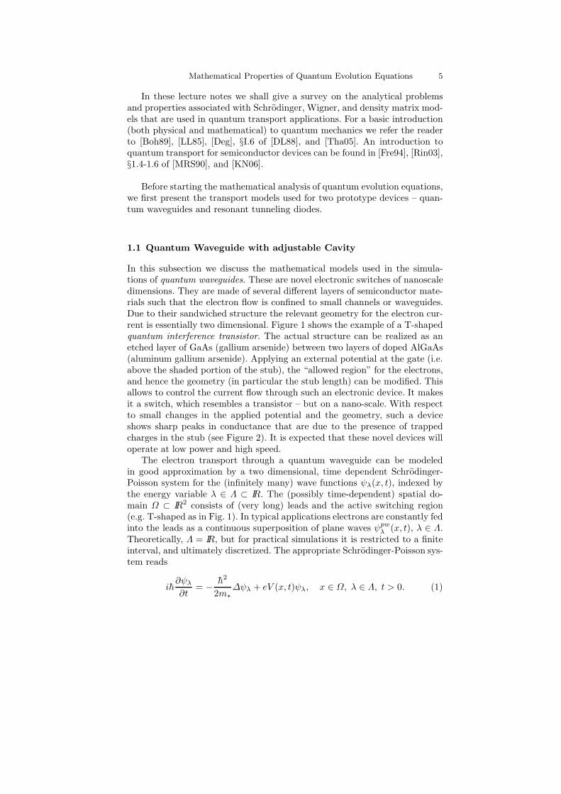
In this subsection we discuss the mathematical models used in the simula-tions of quantum waveguides. These are novel electronic switches of nanoscaledimensions. They are made of several different layers of semiconductor mate-rials such that the electron flow is confined to small channels or waveguides.Due to their sandwiched structure the relevant geometry for the electron cur-rent is essentially two dimensional. Figure 1 shows the example of a T-shapedquantum interference transistor. The actual structure can be realized as anetched layer of GaAs (gallium arsenide) between two layers of doped AlGaAs(aluminum gallium arsenide). Applying an external potential at the gate (i.e.above the shaded portion of the stub), the “allowed region” for the electrons,and hence the geometry (in particular the stub length) can be modified. Thisallows to control the current flow through such an electronic device. It makesit a switch, which resembles a transistor – but on a nano-scale. With respectto small changes in the applied potential and the geometry, such a deviceshows sharp peaks in conductance that are due to the presence of trappedcharges in the stub (see Figure 2). It is expected that these novel devices willoperate at low power and high speed.
The electron transport through a quantum waveguide can be modeledin good approximation by a two dimensional, time dependent Schrodinger-Poisson system for the (infinitely many) wave functions ψλ(x, t), indexed bythe energy variable λ ∈ Λ ⊂ IR. The (possibly time-dependent) spatial do-main Ω ⊂ IR2 consists of (very long) leads and the active switching region(e.g. T-shaped as in Fig. 1). In typical applications electrons are constantly fedinto the leads as a continuous superposition of plane waves ψpwλ (x, t), λ ∈ Λ.Theoretically, Λ = IR, but for practical simulations it is restricted to a finiteinterval, and ultimately discretized. The appropriate Schrodinger-Poisson sys-tem reads
ih∂ψλ∂t
= − h2
2m∗∆ψλ + eV (x, t)ψλ, x ∈ Ω, λ ∈ Λ, t > 0. (1)
6 Anton Arnold
0 X
0
Y1
Y3
ψInc
w
Y2
x
y
L2
L1
Fig. 1. T-shaped geometry Ω ⊂ IR2 of a quantum interference transistor with sourceand drain contacts to the left and right of the channel. Applying a gate voltage abovethe stub allows to modify the stub length from L1 to L2 and hence to switch thetransistor between the on- and off-states. In numerical simulations, the domain Ω isartificially cut off at x = 0 and x = X by adding transparent boundary conditions.
Here, h is the reduced Planck constant, m∗ the effective electron mass in thesemiconductor crystal lattice, and e denotes the (positive) elementary charge.The potential V = Ve + Vsc consists of an external, applied potential Veand the selfconsistent potential satisfying the Poisson equation with Dirichletboundary conditions:
−ε∆Vsc(x, t) = e n(x, t) = e
∫
Λ
|ψλ(x, t)|2g(λ) dλ, x ∈ Ω, (2)
Vs = 0, on ∂Ω.
Here, ε is the permittivity of the semiconductor material and n the spatialelectron density. g(λ) is a probability distribution, representing the statistics(Fermi-Dirac, e.g.) of the injected waves from both the left and right contact.
In this model we made the following simplifications: We considered onlya single band and the Schrodinger equation is in the effective mass approxi-mation. This means that the effect of the microscopic crystal lattice (yieldinga highly oscillatory potential on the atomic length scale) is assumed to behomogenized, and this results in the (constant) effective mass m∗. In het-erostructures, however, the effective mass might be space dependent, or eveninduce nonlocal effects.
This quantum waveguide is connected via leads to an electric circuit.Hence, it is an open system with current flowing through the device. As a
Mathematical Properties of Quantum Evolution Equations 7
consequence, the total electron mass inside the system does not stay con-stant in time. In typical applications the two leads or contact regions aremuch longer than suggested by Figure 1. To reduce computational costs oneis therefore obliged to reduce the simulation domain by introducing so-calledopen or transparent boundary conditions (TBCs), at x = 0 and x = X . Thepurpose of such TBCs is to cut-off the computational domain, but withoutchanging the solution of the original equation. In the simplest case (i.e. a 1Dapproximation and V ≡ 0 in the leads) the TBC takes the form
∂
∂η(ψλ−ψpwλ ) = −
√
2m∗
he−iπ/4
√
∂t (ψλ−ψpwλ ), for λ ∈ Λ, x = 0 or x = X,
(3)where η denotes the unit outward normal vector at each interface.
öt is
the fractional time derivative of order 12 , and it can be rewritten as a time-
convolution of the boundary data with the kernel t−3/2. For the derivation ofthe 2D-variant of such TBCs and the mathematical analysis of this coupledmodel (1)-(3) we refer to [BMP05, Arn01, AABES07] and to [LK90] for astationary Schrodinger-TBC.
To close this subsection we present some simulations of the electron flowthrough the T-shaped waveguide from Figure 1 with the dimensions X = 60nm, Y1 = 20 nm. These calculations are based on the linear Schrodingerequation for a single wave function with V ≡ 0 and the injection of a mono-energetic plane wave (i.e. Λ = λ0) with λ0=130 meV from the left lead.The corresponding function ψpwλ0
(t) then appears in formula (3) for the leftTBC at x = 0. The simulation was based on a compact forth order finitedifference scheme (“Numerov scheme”) and a Crank-Nicolson discretizationin time [AS07, SA07, AJ06].
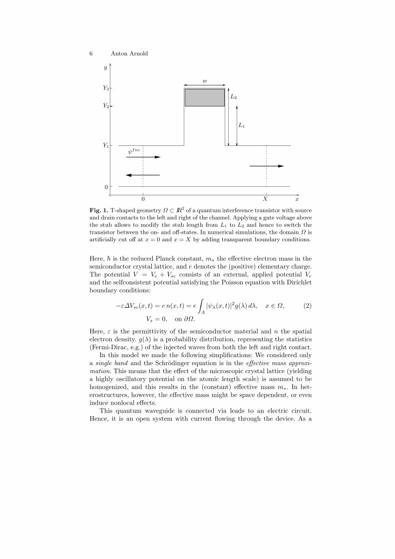
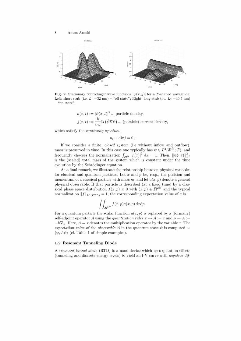
There are two important device data for practitioners: the current-voltage(I-V) characteristics and the ratio between the on- and the (residual) off-current. This information can be obtained from computing the stationarySchrodinger states from the time independent analogue of (1)-(3). Moreover, athird important parameter is the switching time between these two stationarystates. Depending on the size and shape of the stub, the electron current iseither reflected (“off-state” of the device, see Fig. 2, left) or it can flow throughthe device (“on-state”, see Fig. 2, right). In a numerical simulation, this deviceswitching can be realized as follows. Starting from the stationary Schrodingerstate shown in Fig. 2 left, we instantaneously extended the stub length fromL1 = 32 nm to L2 = 40.5 nm. This initiates an evolution of the wave function.After a transient phase of about 4 ps, the new steady state (cf. Fig. 2, right)is reached.
The (complex valued) Schrodinger wave function ψ(x, t), obtained from(1) is rather an auxiliary quantity without intrinsic physical interpretation.Instead, one is rather interested in the following macroscopic quantities :
8 Anton Arnold
0
20
40
60
010
2030
4050
60
0
0.5
1
1.5
2
2.5
3
y [nm]
t = 2500⋅ ∆ t
x [nm]
|ψ(x
,y,t)
|
0
20
40
60
0 10
2030
4050
60
0
0.5
1
1.5
2
2.5
3
x [nm]
t = 7600 ⋅ ∆ t
y [nm]
|ψ(x
,y,t)
|
Fig. 2. Stationary Schrodinger wave functions |ψ(x, y)| for a T -shaped waveguide.Left: short stub (i.e. L1 =32 nm) – “off state”; Right: long stub (i.e. L2 =40.5 nm)– “on state”.
n(x, t) := |ψ(x, t)|2 ... particle density,
j(x, t) :=h
m∗ℑ
(ψ∇ψ
)... (particle) current density,
which satisfy the continuity equation:
nt + divj = 0 .
If we consider a finite, closed system (i.e without inflow and outflow),mass is preserved in time. In this case one typically has ψ ∈ L2(IRN ;CI ), and
frequently chooses the normalization∫
IRN |ψ(x)|2 dx = 1. Then, ‖ψ(·, t)‖2L2
is the (scaled) total mass of the system which is constant under the timeevolution by the Schrodinger equation.
As a final remark, we illustrate the relationship between physical variablesfor classical and quantum particles. Let x and p be, resp., the position andmomentum of a classical particle with massm, and let a(x, p) denote a generalphysical observable. If that particle is described (at a fixed time) by a clas-sical phase space distribution f(x, p) ≥ 0 with (x, p) ∈ IR2N and the typicalnormalization ‖f‖L1(IR2N ) = 1, the corresponding expectation value of a is
∫ ∫
IR2N
f(x, p)a(x, p) dxdp .
For a quantum particle the scalar function a(x, p) is replaced by a (formally)self-adjoint operator A using the quantization rules x 7→ A := x and p 7→ A :=−h∇x. Here, A = x denotes the multiplication operator by the variable x. Theexpectation value of the observable A in the quantum state ψ is computed as〈ψ,Aψ〉 (cf. Table 1 of simple examples).
1.2 Resonant Tunneling Diode
A resonant tunnel diode (RTD) is a nano-device which uses quantum effects(tunneling and discrete energy levels) to yield an I-V curve with negative dif-
Mathematical Properties of Quantum Evolution Equations 9
Table 1. Examples of the quantization rule.
classical quantity, quantization, expectation valuea(x, p) operator A 〈ψ,Aψ〉
x ... position xRx |ψ|2 dx
p ... momentum −ih∇x ihRψ∇ψ dx
|p|2
2m... kinetic energy − h2
2m∆x
h2
2m
R|∇ψ|2 dx
V (x) ... potential (energy) V (x)RV (x)|ψ|2 dx
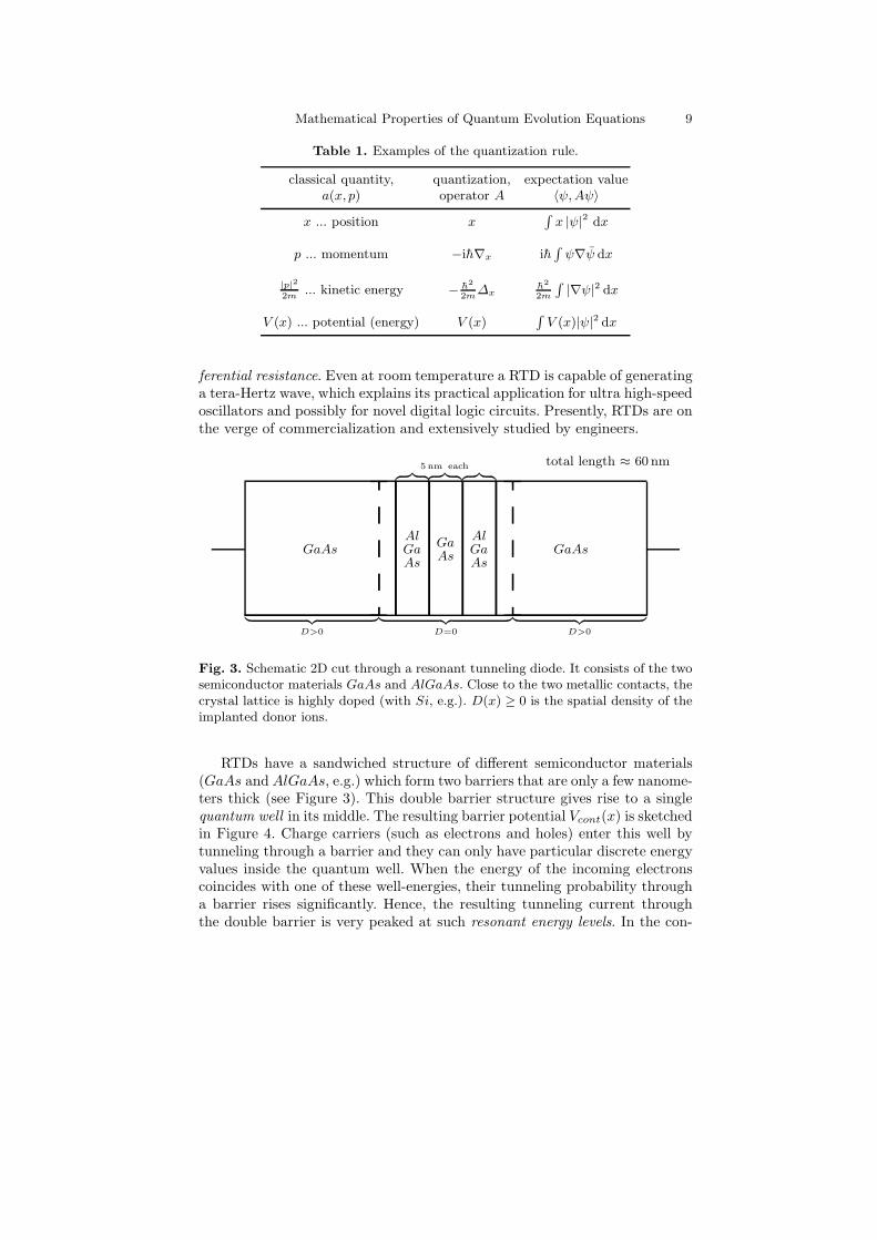
ferential resistance. Even at room temperature a RTD is capable of generatinga tera-Hertz wave, which explains its practical application for ultra high-speedoscillators and possibly for novel digital logic circuits. Presently, RTDs are onthe verge of commercialization and extensively studied by engineers.
GaAsAlGaAs
GaAs
AlGaAs
GaAs
z | 5 nm each
z | z |
| z
D>0
| z
D=0
| z
D>0
total length ≈ 60 nm
Fig. 3. Schematic 2D cut through a resonant tunneling diode. It consists of the twosemiconductor materials GaAs and AlGaAs. Close to the two metallic contacts, thecrystal lattice is highly doped (with Si, e.g.). D(x) ≥ 0 is the spatial density of theimplanted donor ions.
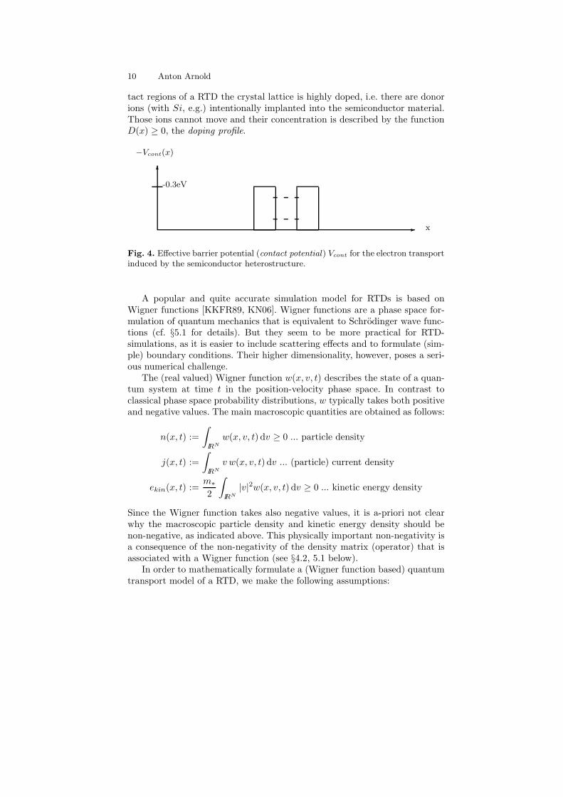
RTDs have a sandwiched structure of different semiconductor materials(GaAs and AlGaAs, e.g.) which form two barriers that are only a few nanome-ters thick (see Figure 3). This double barrier structure gives rise to a singlequantum well in its middle. The resulting barrier potential Vcont(x) is sketchedin Figure 4. Charge carriers (such as electrons and holes) enter this well bytunneling through a barrier and they can only have particular discrete energyvalues inside the quantum well. When the energy of the incoming electronscoincides with one of these well-energies, their tunneling probability througha barrier rises significantly. Hence, the resulting tunneling current throughthe double barrier is very peaked at such resonant energy levels. In the con-
10 Anton Arnold
tact regions of a RTD the crystal lattice is highly doped, i.e. there are donorions (with Si, e.g.) intentionally implanted into the semiconductor material.Those ions cannot move and their concentration is described by the functionD(x) ≥ 0, the doping profile.
- x
6
−Vcont(x)
-0.3eV
Fig. 4. Effective barrier potential (contact potential) Vcont for the electron transportinduced by the semiconductor heterostructure.
A popular and quite accurate simulation model for RTDs is based onWigner functions [KKFR89, KN06]. Wigner functions are a phase space for-mulation of quantum mechanics that is equivalent to Schrodinger wave func-tions (cf. §5.1 for details). But they seem to be more practical for RTD-simulations, as it is easier to include scattering effects and to formulate (sim-ple) boundary conditions. Their higher dimensionality, however, poses a seri-ous numerical challenge.
The (real valued) Wigner function w(x, v, t) describes the state of a quan-tum system at time t in the position-velocity phase space. In contrast toclassical phase space probability distributions, w typically takes both positiveand negative values. The main macroscopic quantities are obtained as follows:
n(x, t) :=
∫
IRN
w(x, v, t) dv ≥ 0 ... particle density
j(x, t) :=
∫
IRN
v w(x, v, t) dv ... (particle) current density
ekin(x, t) :=m∗
2
∫
IRN
|v|2w(x, v, t) dv ≥ 0 ... kinetic energy density
Since the Wigner function takes also negative values, it is a-priori not clearwhy the macroscopic particle density and kinetic energy density should benon-negative, as indicated above. This physically important non-negativity isa consequence of the non-negativity of the density matrix (operator) that isassociated with a Wigner function (see §4.2, 5.1 below).
In order to mathematically formulate a (Wigner function based) quantumtransport model of a RTD, we make the following assumptions:
Mathematical Properties of Quantum Evolution Equations 11
• only one carrier species is considered: electrons (since the mobility of theholes is too small in such a device to contribute significantly to the chargetransport)
• one-particle-like mean field model (Hartree approximation)• only one parabolic band (with effective mass m∗)• purely quantum mechanical transport• ballistics dominates scattering effects (for device lengths up to the order
of the electrons’ mean free path)
Under the above assumptions, the Wigner equation describes the time evo-lution of the Wigner function w in a given, real valued (electrostatic) potentialV (x, t):
wt + v · ∇xw − eΘ[V ]w = 0, x, v ∈ IRN . (4)
Here, Θ[V ] is a pseudo-differential operator (typical abbreviation: “ΨDO”),defined via a multiplication operator for the v-Fourier transformed Wignerfunction Fvw:
Θ[V ]w(x, v)
=i
h(2π)−N
∫∫
IR2N
[
V (x +hη
2m∗) − V (x− hη
2m∗)
]
w(x, v)ei(v−v)·η dvdη .
Under some regularity and decay assumptions on the potential V , it can berewritten as convolution operator in v:
Θ[V ]w(x, v) = α(x, v) ∗v w(x, v)
α(x, v) :=2
h(2π)−
N2
(2m∗
h
)N
ℑ[
ei 2m∗hx·v
(FV
)(
2m∗
hv
)]
.
This convolution form illustrates the non-local effect of potentials in quantummechanics. Indeed, a particle or wave packet already “feels” an upcomingpotential barrier before actually hitting it. Such a “premature” reflection isclearly seen in numerical simulations based on Wigner functions.
For realistic device simulations, scattering (between electrons and impu-rities or with phonons, i.e. thermal vibrations of the crystal lattice) must beincluded in the model. Hence, the r.h.s. of (4) has to be augmented by some (atleast simple) scattering term. For the 1D simulations of a RTD in [KKFR89]the following relaxation term was used as a phenomenological model for theelectron–phonon interactions:
wt + vwx − eΘ [Vsc(x, t) + Vcont(x)]w =wst − w
τ(v), (5)
0 < x < L, v ∈ IR, t > 0.
Here, wst is some appropriate steady state, and τ > 0 denotes the relaxationtime, which may be energy dependent. The spatial interval (0, L) models the
12 Anton Arnold
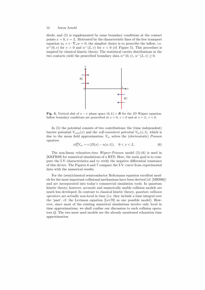
diode, and (5) is supplemented by some boundary conditions at the contactpoints x = 0, x = L. Motivated by the characteristic lines of the free transportequation wt + v · ∇xw = 0, the simplest choice is to prescribe the inflow, i.e.w+(0, v) for v > 0 and w−(L, v) for v < 0 (cf. Figure 5). This procedure isinspired by classical kinetic theory. The statistical carrier distributions in thetwo contacts yield the prescribed boundary data w+(0, v), w−(L, v) ≥ 0.
Lxo
BC
v
BC
Fig. 5. Vertical slab of x − v–phase space (0, L) × IR for the 1D Wigner equation:Inflow boundary conditions are prescribed at x = 0, v > 0 and at x = L, v < 0.
In (5) the potential consists of two contributions: the (time independent)barrier potential Vcont(x) and the self-consistent potential Vsc(x, t), which isdue to the mean field approximation. Vsc solves the (electrostatic) Poissonequation
ε∂2xVsc = e (D(x) − n(x, t)), 0 < x < L . (6)
The non-linear relaxation-time Wigner-Poisson model (5)-(6) is used in[KKFR89] for numerical simulations of a RTD. Here, the main goal is to com-pute the I-V–characteristics and to verify the negative differential resistanceof this device. The Figures 6 and 7 compare the I-V–curve from experimentaldata with the numerical results.
For the (semi)classical semiconductor Boltzmann equation excellent mod-els for the most important collisional mechanisms have been derived (cf. [MRS90])and are incorporated into today’s commercial simulation tools. In quantumkinetic theory, however, accurate and numerically usable collision models aremuch less developed. In contrast to classical kinetic theory, quantum collisionoperators are actually non-local in time (i.e. they include a time integral overthe ‘past’, cf. the Levinson equation [Lev70] as one possible model). How-ever, since most of the existing numerical simulations involve only local intime approximations, we shall confine our discussion to such collision opera-tors Q. The two most used models are the already mentioned relaxation timeapproximation

Mathematical Properties of Quantum Evolution Equations 13
Fig. 6. I-V–characteristics of a RT-diode shows negative differential resistance:— experimental data, - - - computed with a simple Schrodinger tunneling model.Reprinted figure with permission from [KKFR89]. Copyright (1989) by the AmericanPhysical Society.
Fig. 7. I-V–characteristics of a RT-diode shows a hysteresis including two stablebranches: numerical simulation based on a relaxation-time Wigner-Poisson model.Reprinted figure with permission from [KKFR89]. Copyright (1989) by the AmericanPhysical Society.
Qw :=wst(x, v) − w(x, v, t)
τ(v)
and the quantum Fokker-Planck model with
Qw := Dpp∆vw︸ ︷︷ ︸
class. diffusion
+ 2γ divv(vw)︸ ︷︷ ︸
friction
+Dqq∆xw + 2Dpq divx(∇vw)︸ ︷︷ ︸
quantum diffusion
(7)
(cf. [CL83, CEFM00] for a derivation). Both of these models are purely phe-nomenological, but quantum mechanically “correct” (if τ(v) = τ0 ≥ 0 or if theLindblad condition (35) holds). And this is important for their mathematicalanalysis (cf. §6.2).
As a third option, the r.h.s. of the Wigner equation (4) is often replacedby a semiclassical Boltzmann scattering operator
Qw :=
∫
IRN
[S(v, v′)w(x, v′) − S(v′, v)w(x, v)] dv′ ,
14 Anton Arnold
with the scattering rate S(v, v′) (for the electron-phonon interaction, e.g.).Such semiclassical Boltzmann operators give good simulation results [KN06],but they are quantum mechanically not “correct” (cf. §6.1). Hence, we shallnot discuss their mathematical analysis.
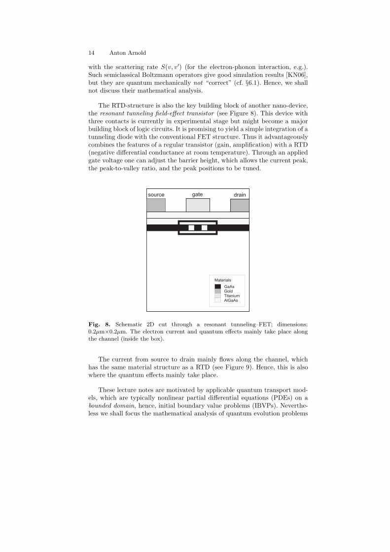
The RTD-structure is also the key building block of another nano-device,the resonant tunneling field-effect transistor (see Figure 8). This device withthree contacts is currently in experimental stage but might become a majorbuilding block of logic circuits. It is promising to yield a simple integration of atunneling diode with the conventional FET structure. Thus it advantageouslycombines the features of a regular transistor (gain, amplification) with a RTD(negative differential conductance at room temperature). Through an appliedgate voltage one can adjust the barrier height, which allows the current peak,the peak-to-valley ratio, and the peak positions to be tuned.
Materials
GaAsGoldTitaniumAlGaAs
source gate drain
Fig. 8. Schematic 2D cut through a resonant tunneling–FET; dimensions:0.2µm×0.2µm. The electron current and quantum effects mainly take place alongthe channel (inside the box).
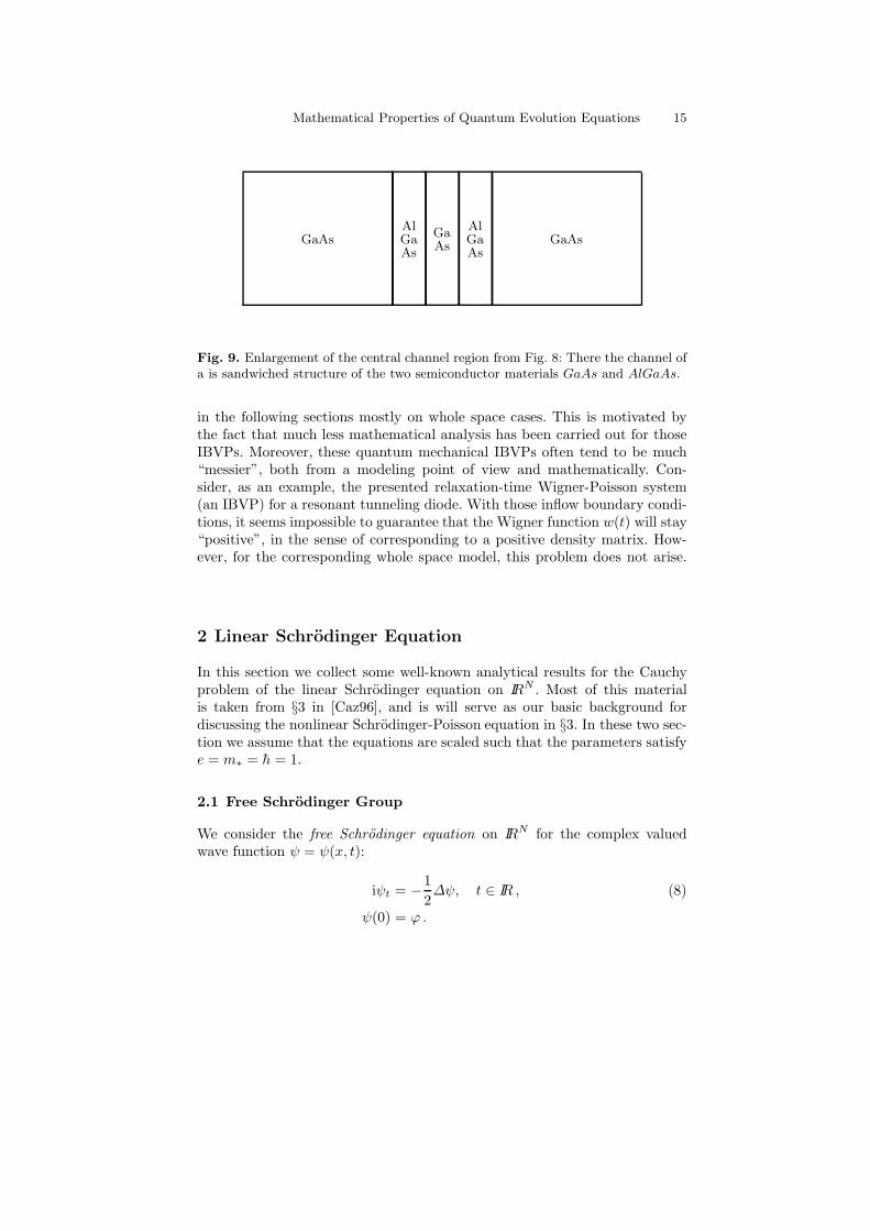
The current from source to drain mainly flows along the channel, whichhas the same material structure as a RTD (see Figure 9). Hence, this is alsowhere the quantum effects mainly take place.
These lecture notes are motivated by applicable quantum transport mod-els, which are typically nonlinear partial differential equations (PDEs) on abounded domain, hence, initial boundary value problems (IBVPs). Neverthe-less we shall focus the mathematical analysis of quantum evolution problems
Mathematical Properties of Quantum Evolution Equations 15
GaAsAlGaAs
GaAs
AlGaAs
GaAs
Fig. 9. Enlargement of the central channel region from Fig. 8: There the channel ofa is sandwiched structure of the two semiconductor materials GaAs and AlGaAs.
in the following sections mostly on whole space cases. This is motivated bythe fact that much less mathematical analysis has been carried out for thoseIBVPs. Moreover, these quantum mechanical IBVPs often tend to be much“messier”, both from a modeling point of view and mathematically. Con-sider, as an example, the presented relaxation-time Wigner-Poisson system(an IBVP) for a resonant tunneling diode. With those inflow boundary condi-tions, it seems impossible to guarantee that the Wigner function w(t) will stay“positive”, in the sense of corresponding to a positive density matrix. How-ever, for the corresponding whole space model, this problem does not arise.
2 Linear Schrodinger Equation
In this section we collect some well-known analytical results for the Cauchyproblem of the linear Schrodinger equation on IRN . Most of this materialis taken from §3 in [Caz96], and is will serve as our basic background fordiscussing the nonlinear Schrodinger-Poisson equation in §3. In these two sec-tion we assume that the equations are scaled such that the parameters satisfye = m∗ = h = 1.
2.1 Free Schrodinger Group
We consider the free Schrodinger equation on IRN for the complex valuedwave function ψ = ψ(x, t):
iψt = −1
2∆ψ, t ∈ IR , (8)
ψ(0) = ϕ .
16 Anton Arnold
The operator A := 12∆ with the domain D(A) = H2(RN) is self-adjoint
on L2(IRN ). By Stone’s Theorem (cf. [Paz83]) iA hence generates a C0–groupof isometries on L2(IRN ):
T (t), t ∈ IR; T (t)∗ = T (−t)
T (t1)T (t2) = T (t1+t2), T (0) = I
limt→0
T (t)ϕ = ϕ ∀ϕ ∈ L2(IRN )
limt→0
T (t)ϕ− ϕ
t= iAϕ ∀ϕ ∈ D(A)
The operator iA is call the infinitesimal generator of T (t). This evolutiongroup provides a solution to (8) in the following sense:
Proposition 2.1.
(a) Let ϕ ∈ L2(IRN ). Then ψ(t) = T (t)ϕ is the unique solution of
iψt = − 12∆ψ in H−2(IRN ), ∀t ∈ IR
ψ ∈ C(IR;L2(IRN )) ∩C1(IR;H−2(IRN ))ψ(0) = ϕ
This mild solution satisfies mass conservation, i.e. ‖ψ(t)‖L2 = ‖ϕ‖L2 ∀t ∈IR (since T (t) is isometric).
(b) If ϕ ∈ H2(IRN ), the above solution is a classical solution with ψ ∈C(IR;H2) ∩ C1(IR;L2) .
Lemma 2.2 (Representation of T (t)).
T (t)ϕ = K(t) ∗ ϕ ∀t 6= 0, ϕ ∈ S(IRN ) (9)
K(x, t) = (8πit)−N2 e
i|x|2
8t
Proof. Define ψ ∈ C(IR;S(IRN )) by:
ψ(ξ, t) := e−i
2|ξ|2t
︸ ︷︷ ︸
=K(ξ,t)
ϕ(ξ), ξ ∈ IRN (10)
⇒ iψt =1
2|ξ|2ψ on IRt × IRN
ψ(0) = ϕ(ξ)
⊓⊔
Note the (formal) similarity between K(x, t), the Green’s function of theSchrodinger equation and the heat kernel.
For more regular initial data, the regularity is propagated in time:
Mathematical Properties of Quantum Evolution Equations 17
Remark 2.3.
(a) Let ϕ ∈ Hs(IRN ), s ∈ IR. Then ψ(t) = T (t)ϕ satisfies:
ψ ∈⋂
0≤j<∞
Cj(IR;Hs−2j(IRN )), ‖ψ(t)‖Hs = ‖ϕ‖Hs .
This follows from (10) with ‖ϕ‖2Hs =
∥∥∥
(1 + |ξ|2
) s2 ϕ(ξ)
∥∥∥
2
L2
.
(b)
T (t)ϕ = (8πit)−N2 e
i|x|2
8t
∫
IRN
e−ix·y4t e
i|y|2
8t ϕ(y) dy, t 6= 0 . (11)
I.e. T (t) is a Fourier transform up to a rescaling and a multiplication bya function of modulus 1.
2.2 Smoothing Effects and Gain of Integrability in IRN
We shall now discuss simple smoothing properties of the free Schrodingergroup T (t). On the one hand we can gain local integrability for t 6= 0. On theother hand, (11) shows that T (t), t 6= 0 is almost a Fourier transform. Anda Fourier transform maps nicely decaying functions into smooth functions.However, the regularity gain for t 6= 0 never appears directly on ψ, but it isalways coupled to some spatial moments of ψ. This is caused by the multiplier
ei|y|2
8t in (11):
Proposition 2.4. Let the multi-index α ∈ INN0 , ϕ ∈ S′(IRN ) with xαϕ ∈
L2(IRN ), and let ψ(t) = T (t)ϕ ∈ C(IR;S ′(IRN )). Then
∂αx
(
e−i|x|2
8t ψ(t)
)
∈ C(IR\0;L2(IRN )),
(4|t|)|α|∥∥∥∥∂αx
(
e−i|x|2
8t ψ(t)
)∥∥∥∥L2
= ‖xαϕ‖L2 , t ∈ IR .
This follows directly from (11).
Example 2.5. Choose |α| = 1:
‖(x+ 4i t∇)ψ(t)‖L2 = const = ‖xϕ‖L2 , t ∈ IR .
Now we consider the gain of local-in-x integrability:
Proposition 2.6. Let 2 ≤ p ≤ ∞, t 6= 0. Then T (t) ∈ B(Lp′
(IRN ), Lp(IRN )):
‖T (t)ϕ‖Lp ≤ (8π|t|)−N( 1
2− 1
p) ‖ϕ‖Lp′ ∀ϕ ∈ Lp′
(IRN ) . (12)
Here and in the sequel p′ = pp−1 is the Holder conjugate of p.
18 Anton Arnold
Proof. Let ϕ ∈ S(IRN):
‖T (t)ϕ‖L∞ ≤ (8π|t|)−N2 ‖ϕ‖L1 follows from (9) by the Young inequality
for convolutions,
‖T (t)ϕ‖L2 = ‖ϕ‖L2 since T (t) is isometric.
The result then follows by interpolation (Riesz-Thorin Theorem, [RS75]) andthe density of S(IRN ) in Lp
′
(IRN ). ⊓⊔
2.3 Potentials, Inhomogeneous Equation
Here, we first discuss homogeneous Schrodinger equations with bounded andrelatively bounded potentials:
Proposition 2.7 (Bounded perturbations of generators, [Paz83]). LetA be the infinitesimal generator of the C0–semigroup T (t) on the Banach spaceX with ‖T (t)‖ ≤Meωt, and B ∈ B(X).Then A+B generates a C0–semigroup S(t) on X with
‖S(t)‖ ≤Me(ω+M‖B‖)t, t ∈ IR .
Example 2.8. Schrodinger equation with bounded potential V ∈ L∞(IRN ):
iψt = − 1
2∆ψ + V ψ, t ∈ IR
ψ(0) = ϕ ∈ L2(IRN )
has a unique mild solution. It is even a classical solution for ϕ ∈ H2(IRN ).The Hamiltonian of this equation is H := − 1
2∆ + V . It reveals conservationof the following energy:
〈ψ(t), Hψ(t)〉 =1
2‖∇ψ(t)‖2
L2 +
∫
IRN
V n(t) dx = const in t . (13)
Next we perturb the free Hamiltonian by a special class of unboundedpotentials:
Proposition 2.9 (Relatively bounded perturbations of generators,Kato-Rellich Th. [RS75]). Let A be a self-adjoint operator on the Hilbertspace X, and the operator B symmetric and A–bounded (i.e.
∃a, b ∈ IR : ‖Bϕ‖ < a‖Aϕ‖ + b‖ϕ‖ ∀ϕ ∈ D(A) )
with a < 1. Then A+B is self-adjoint on D(A).
Mathematical Properties of Quantum Evolution Equations 19
Example 2.10. Hydrogen atom — motion of one electron in the attractiveCoulomb potential of the fixed nucleus:
iψt = − 1
2∆ψ − 1|x|ψ, t ∈ IR
ψ(0) = ϕ ∈ L2(IR3) (or ϕ ∈ H2(IR3))
has a unique mild (or, resp., classical) solution. To prove this, we split thepotential V (x) = 1
|x| into a short and long range potential:
V = V1 + V2 with
V1 ∈ L2(IR3), V2 := min
(
1,1
|x|
)
∈ L∞(IR3) .
V1 is ∆–bounded because of ψ ∈ H2(IR3) → L∞(IR3) by a Sobolev embed-ding. Hence, Proposition 2.9 applies to V1 and Proposition 2.7 applies to V2.
Now we turn to inhomogeneous Schrodinger equations:
Proposition 2.11. Let ϕ ∈ L2(IRN), f ∈ C([0, T ];L2(IRN )).
(a) Then ∃! solution of
iψt + 12∆ψ + f = 0 ∀t ∈ [0, T ]
ψ ∈ C([0, T ];L2(IRN )) ∩C1([0, T ];H−2(IRN ))ψ(0) = ϕ .
With T (t) denoting the free Schrodinger group, this mild solution satisfies
ψ(t) = T (t)ϕ+ i
∫ t
0
T (t− s)f(s) ds, 0 ≤ t ≤ T. (14)
(b) Let, additionally, ϕ ∈ H2(IRN ) and either f ∈ W 1,1((0, T );L2(IRN )) orf ∈ L1((0, T );H2(IRN )). Then ψ is a ( classical solution), satisfying ψ ∈C(IR;H2) ∩ C1(IR;L2) .
2.4 Strichartz Estimates
The goal of this subsection is to derive combined space-time estimates for theinhomogeneous Schrodinger equation (14).
Definition 2.12. A pair of indices (q, p) is called admissible if
2 ≤ p < 2NN−2 (or 2 ≤ p ≤ ∞ if N = 1; 2 ≤ p <∞ if N = 2),
2q = N(1
2 − 1p ) .
20 Anton Arnold
Notation:
Lq,p := Lq(IRt;Lp(IRN ))
Lq,pI := Lq(I;Lp(IRN )) for any interval I ⊂ IR
The following Strichartz estimate for the free and inhomogeneous Schro-dinger equation describes a gain of local-in-x integrability. Since the followinginequalities hold in a mixed space-time norm, this gain of integrability doesnot hold pointwise in time, but for almost all t:
Proposition 2.13. Let (q, p), (a, b) be admissible pairs.
(a) Let ϕ ∈ L2(IRN ). Then T (t)ϕ ∈ Lq,p ∩ C(IR;L2(IRN )) with
‖T (·)ϕ‖Lq,p ≤ C(q)‖ϕ‖L2 . (15)
(b) Let f ∈ La′,b′
I and t0 ∈ I. Then it holds
Λf (t) :=
∫ t
t0
T (t− s)f(s) ds ∈ Lq,pI ∩ C(I;L2(IRN ))
with‖Λf‖Lq,p
I≤ C(a, q)‖f‖
La′,b′
I
.
The constants C(q) and C(a, q) are independent of time.
Proof (of the inhomogeneous version for (a, b) = (q, p). The general case de-pends on duality arguments, see §3.2 of [Caz96]).
Let I = [0, T ], t0 = 0, f ∈ Cc([0, T ];Lp′
); the result for general f ∈ Lq,p thenfollows by density. Inequality (12) and N(1
2 − 1p ) = 2
q yield:
‖Λf (t)‖Lp ≤ C(q)
∫ t
0
|t− s|−N( 1
2− 1
p)‖f(s)‖Lp′ ds
≤ C(p)
∫ T
0
|t− s|− 2
q ‖f(s)‖Lp′ ds .
With the weak Young inequality (cf. [RS75]) we conclude:
‖Λf‖Lq,p
I≤ C(q)‖f‖
Lq′,p′
I
.
⊓⊔
Remark 2.14.
(a) In Prop. 2.13(a) ϕ ∈ L2(IRN ) implies T (t)ϕ ∈ Lp for almost all t ∈ IR(for p > 2). It cannot be improved to “for all t 6= 0”.
Mathematical Properties of Quantum Evolution Equations 21
(b) Since the Schrodinger equation is time reversible, the presented smoothingeffects are much more subtle than for the heat equation. The evolutionalso improves the local integrability of the solution ψ for almost all t. Thesmoothing effects in Prop. 2.6 and Prop. 2.13 are due to the dispersionin the Schrodinger equation. This means that waves of different frequen-cies (or wavelengths) travel at different velocities, when decomposing thesolution ψ into plane waves..
(c) A remarkable aspect of Prop. 2.13(b) is that the index pairs (q, p) and(a′, b′) are uncorrelated.
3 Schrodinger-Poisson analysis in IR3
The goal of this section is to prove that the repulsive Schrodinger-Poisson (SP)equation (or Hartree equation) in IR3 has a unique, global-in-time solution,first for initial data in H1 and then in L2. We shall mostly follow §6.3 of[Caz96] and [Cas97]; but see also [GV94, HO89]. We remark that extensionsof this analysis to the Sobolev spaces Hk, k ≥ 2 is straightforward [Caz96].Extensions to space dimensions N 6= 3 require some modifications, since theused Sobolev embeddings depend on N [Caz96, AN91].
3.1 H1–analysis
A wave function ψ ∈ H1 corresponds to a system with finite mass ‖ψ‖2L2 and
finite kinetic energy 12‖∇ψ‖2
L2 . As we shall see, this property is propagated intime.
In the sequel we shall frequently need the following result on solutionsto nonlinear Banach space–ODEs (i.e. an ordinary differential equation for aBanach space–valued function):
Proposition 3.1 (Local Lipschitz perturbations of generators).[Paz83] Let A be the infinitesimal generator of the C0–semigroup T (t), t ≥ 0on the Banach space X, and let f = f(t, u) : [0,∞) ×X → X be continuousin t and locally Lipschitz in u (uniformly in t on bounded intervals).
(a) Then, ∀ϕ ∈ X, ∃tmax = tmax(ϕ) ≤ ∞:
dudt = Au+ f(t, u(t)), t ≥ 0u(0) = ϕ
has a unique mild solution u ∈ C([0, tmax);X).(b) If tmax <∞ then limtրtmax
‖u(t)‖X = ∞, i.e. blow-up in finite time.(b’) If ‖u(t)‖X <∞ ∀t ∈ [0,∞) ⇒ The solution exists global-in-time.
This theorem will now be applied to the repulsive Schrodinger-Poisson equa-tion (or Hartree equation):
22 Anton Arnold
iψt = − 12∆ψ + V ψ, x ∈ IR3, t ∈ IR
−∆xV (x, t) = n(x, t) := |ψ(x, t)|2ψ(0) = ϕ
(16)
We take the Newton potential solution of the Poisson equation:
V = 14π|x| ∗ |ψ|2
∇V = − x4π|x|3 ∗ |ψ|2 (17)
Theorem 3.2. Let ϕ ∈ H1(IR3). Then (16) has a unique solution ψ ∈C(IR;H1(IR3)).
Proof.
1. T (t) = ei
2∆t is a C0–group of isometries both on L2(IR3) and H1(IR3).
2. f(ψ) := −iV [ψ]ψ = −i(
14π|x| ∗ |ψ|2
)
ψ is locally Lipschitz in H1 (but not
in L2; hence we analyze (16) in H1) since:The weak Young inequality (cf. [RS75]) for (17) yields:
‖V ‖Lp ≤ C‖ψ‖2Lq , 3 < p ≤ ∞, 1
p = 2q − 2
3 ,
‖∇V ‖Lp ≤ C‖ψ‖2Lq , 2
3 < p <∞, 1p = 2
q − 13 ,
(18)
and Holder’s inequality and the Sobolev embedding H1(IR3) → L6(IR3)yield:
‖f(ψ)‖L2 ≤ ‖V ‖L∞‖ψ‖L2 ≤ C‖ψ‖3H1 ,
‖∇f(ψ)‖L2 ≤ ‖V ‖L∞‖∇ψ‖L2 + ‖∇V ‖L3‖ψ‖L6 ≤ C‖ψ‖3H1 .
3. By Prop. 3.1 it holds: The Schrodinger-Poisson equation (16) has a uniquelocal solution ψ ∈ C([0, tmax);H
1(IR3)).4. ‖ψ‖H1 cannot blow up in finite time because of the following two esti-
mates:(a) L2–a priori estimate (mass conservation):
The Schrodinger equation (16) holds in C([0, tmax);H−1). We test it
against ψ(t) ∈ H1:
i〈ψt, ψ〉 =1
2‖∇ψ‖2
L2 +
∫
IR3
V |ψ|2 dx .
Taking the imaginary part yields: ddt‖ψ‖2
L2 = 0 .
(b) H1–a priori estimate (energy conservation):We test the Schrodinger equation (16) against ψt and integrate byparts. A formal calculation yields:
i‖ψt‖2L2 =
1
2
∫
IR3
∇ψ · ∇ψt dx+
∫
IR3
V ψψt dx .
Taking the real part and using the Poisson equation yield:
Mathematical Properties of Quantum Evolution Equations 23
0 = 12
ddt‖∇ψ‖2
L2 +∫
IR3 V nt dx = 12
ddt‖∇ψ‖2
L2 +∫
IR3 ∇V · ∇Vt dx
= ddt
[ 1
2‖∇ψ(t)‖2
L2
︸ ︷︷ ︸
kinetic energy
+1
2‖∇V (t)‖2
L2
︸ ︷︷ ︸
self-consist. potential energy
]
Hence, ‖∇ψ(t)‖L2 is uniformly bounded in t.Remark: Here, the (self-consistent) potential energy is 1
2‖∇V ‖2L2 =
12
∫V n dx, while it is
∫V n dx in the linear case (cf. (13)).
5. ⇒ The solution exists ∀t ∈ IR.
⊓⊔
3.2 L2–analysis
If a wave function ψ ∈ L2 but not in H1, the corresponding quantum systemhas finite mass but infinite kinetic energy.
Since the nonlinearity f(ψ) := −iV [ψ]ψ = −i(
14π|x| ∗ |ψ|2
)
ψ is not locally
Lipschitz in L2, our analysis is much more difficult than theH1-analysis above.Here we shall use that f(ψ) is still (somehow) locally Lipschitz in the followingspace of t-dependent functions: Lq,pT := Lq((−T, T );Lp(IR3)), for some fixedT > 0.
We split the self-consistent potential V [ψ] into a short and a long rangepotential: V [ψ] = V1[ψ] + V2[ψ], with V2[ψ] := 1
4π min(1, 1|x|) ∗ |ψ|2. And we
split the nonlinearity f(ψ) analogously: f(ψ) = f1(ψ) + f2(ψ), with fj(ψ) :=−iVj [ψ]ψ.
The following result shows that f1,2(ψ) are locally Lipschitz, however, indifferent spaces Lq,pT .
Lemma 3.3. [Cas97] Let 0 < T < 1; 3 < p < 6; q = q(p) with 2q = 3(1
2 − 1p );
ψ, φ ∈ C([−T, T ];L2(IR3))∩Lq,pT ; M := max[−T,T ](‖ψ(t)‖L2 , ‖φ(t)‖L2). Then
(a)
‖f1(ψ(t)) − f1(φ(t))‖Lq′,p′
T
≤ C(p)M2T 1− 2
q ‖ψ(t) − φ(t)‖Lq,p
T,
(b)
‖f2(ψ(t)) − f2(φ(t))‖L1,2
T≤ CM2T ‖ψ(t)− φ(t)‖L∞,2
T
≤ CM2T 1− 2
q ‖ψ(t) − φ(t)‖L∞,2
T.
Theorem 3.4. Let ϕ ∈ L2(IR3). Then the Schrodinger-Poisson equation (16)has a unique mild solution ψ ∈ C(IR;L2(IR3)) ∩ Lq,ploc with 3 < p < 6, 2
q =
3(12 − 1
p ).
Proof.
24 Anton Arnold
1. Approximating H1–sequence to construct a solution:Let ϕmm∈IN ⊂ H1(IR3) with ϕm
m→∞−→ ϕ in L2, ‖ϕm‖L2 = ‖ϕ‖L2.By Theorem 3.2, for each ϕm, m ∈ IN , the SP-problem then has a uniquesolution ψm ∈ C(IR;H1(R3)), satisfying ‖ψm(t)‖L2 = ‖ϕ‖L2 =: M ∀t ∈IR .
2. ψm(t) is a Cauchy sequence in La,bT for T small:
ψm(t) − ψk(t) = T (t)(ϕm − ϕk)
+∫ t
0 T (t−s)[f1(ψm(s)) − f1(ψk(s))] ds
+∫ t
0 T (t−s)[f2(ψm(s)) − f2(ψk(s))] ds
(19)
The homogeneous Strichartz inequality (Prop. 2.13(a)) yields:
‖T (t)(ϕm − ϕk)‖La,b
T
≤ C(a)‖ϕm − ϕk‖L2 .
The inhomogeneous Strichartz inequality (Prop. 2.13(b)) and Lemma3.3(a) yield for the first nonlinearity:
‖∫ t
0
T (t−s)[f1(ψm(s)) − f1(ψk(s))] ds‖La,b
T
≤ C(a, q)‖f1(ψm(t)) − f1(ψk(t))‖Lq′,p′
T
≤ C(a, q)M2T 1− 2
q ‖ψm(t) − ψk(t)‖Lq,p
T.
Here, (a, b) is any admissible pair.Similarly, the inhomogeneous Strichartz inequality (Prop. 2.13(b)) andLemma 3.3(b) yield for the second nonlinearity:
‖∫ t
0
T (t− s)[f2(ψm(s)) − f2(ψk(s))] ds‖La,b
T
≤ C(a)M2T 1− 2
q ‖ψm(t) − ψk(t)‖L∞,2
T
We collect the last 3 inequalities and add the resulting estimates for thetwo index-choices (a, b) = (q, p), (a, b) = (∞, 2). This yields the followingestimate for (19):
‖ψm(t) − ψk(t)‖Lq,p
T+ ‖ψm(t) − ψk(t)‖L∞,2
T
≤ C(q)‖ϕm − ϕk‖L2
+C(q)M2T 1− 2
q
[
‖ψm(t) − ψk(t)‖Lq,p
T+ ‖ψm(t) − ψk(t)‖L∞,2
T
]
⇒ ∃T0 = T0(q,M) > 0, small enough such that:
‖ψm(t)−ψk(t)‖Lq,p
T0
+‖ψm(t)−ψk(t)‖L∞,2
T0
≤ C(q,M)‖ϕm−ϕk‖L2 . (20)
This implies the following properties of the approximating sequence ψm:
Mathematical Properties of Quantum Evolution Equations 25
• ψm is a Cauchy sequence in Lq,pT0∩ L∞,2
T0
• ψm ⊂ C([−T0, T0];L2(IR3))
• ψm → ψ in Lq,pT0∩ C([−T0, T0];L
2(IR3))• ‖ψm(t)‖L2 = ‖ψ(t)‖L2 = ‖ϕ‖L2 = M, ∀m ∈ IN, ∀t ∈ IR .
Since T0 = T0(q,M) only depends on the index q and M = ‖ϕ‖L2, thesolution ψ can be extended up to 2T0, 3T0, ... , -T0, -2T0, ... Hence, ψ ∈C(IR;L2(IR3)) ∩ Lq,ploc .The estimate (20) also implies uniqueness of the limit ψ and its continuousdependence on the data ϕ. The constructed limit ψ is the mild solutionof (16). To verify this, choose ψk := 0 and pass to the limit (m → ∞) inthe integral equation (19).
⊓⊔
3.3 Schrodinger-Poisson Systems
Up to now we considered just one Schrodinger equation that is coupled to thePoisson equation. This would describe a pure quantum state. In most realisticapplication, however, one has to deal with a mixed quantum state, which canbe described by a sequence of wave functions:
ψj(x, t) ∈ CI , j ∈ IN ; x ∈ IR3, t ∈ IR .
For a system of many particles, this mixed quantum state describes a sta-tistical mixture, and each ψj has an occupation probability λj ≥ 0, j ∈IN ;
∑
j λj = 1. Here, λj are given data and it depends on the initial state ofthe system.
In this section we only consider closed quantum systems, i.e. a systemwithout interaction to an (infinitely large) “environment” or “heat bath”. Itsdynamics is time-reversible and fully described by a Hamiltonian. In this casethe above occupation probabilities λj are constant in time.
Open quantum systems, being the opposite of closed quantum systems willbe discussed in §6.
We consider now the time evolution of this mixed quantum state, givenby the repulsive Schrodinger-Poisson system (SPS):
i ∂∂tψj = − 12∆ψj + V ψj , x ∈ IR3, t ∈ IR, j ∈ IN
V (x, t) = 14π|x| ∗ n(x, t), n(x, t) :=
∑∞j=1 λj |ψj(x, t)|2
ψj(0) = ϕj , j ∈ IN
(21)
In the special case λj := δ1j (δij is the Kronecker-Delta) the SPS reduces to thescalar Hartree equation of §3.1. In the subsequent analysis we follow mostly
26 Anton Arnold
[Cas97].
Notation:For any fixed sequence λ := λjj∈IN ∈ ℓ1 with λj ≥ 0 we define:
H1(λ) := Φ(x) = (ϕj(x))j∈IN , ‖Φ‖2H1(λ) =
∑
j λj‖ϕj(x)‖2H1(IR3) <∞
Lp(λ) := Φ(x) = (ϕj(x))j∈IN , ‖Φ‖2Lp(λ) =
∑
j λj‖ϕj(x)‖2Lp(IR3) <∞
Lq,ploc(λ) := Lqloc(IR;Lp(λ))
Theorem 3.5.
(a) Let Φ ∈ H1(λ). Then (21) has a unique solution Ψ ∈ C(IR;H1(λ)).(b) [Cas97]: Let Φ ∈ L2(λ). Then (21) has a unique mild solution Ψ ∈
C(IR;L2(λ) ∩ Lq,ploc(λ)) for all admissible pairs (q, p) with 3 < p < 6,2q = 3(1
2 − 1p ).
Proof.
(a) This is a straightforward generalization of Theorem 3.2 for the Hartreeequation (cf. [ILZ94], e.g.):
f(Ψ) := −iV [Ψ ]Ψ is locally Lipschitz in H1(λ). The required a-prioriestimates are provided by ‖Ψ(t)‖2
L2(λ) = ‖Φ‖2L2(λ) (mass conservation)
and 12‖∇Ψ(t)‖2
L2(λ) + 12‖∇V (t)‖2
L2 = const. (energy conservation).
(b) This part is based on vector valued Strichartz inequalities for mixed quan-tum states which are non-trivial extensions of Prop. 2.13. E.g., the exten-sion of the homogeneous estimate (15) reads ([Cas97]):
‖T (t)Φ‖Lq,p
T(λ) ≤ C(q, T )‖Φ‖L2(λ) ∀ admissible pairs (q, p)
with
‖T (t)Φ‖qLq,p
T(λ)
=
∫ T
−T
( ∑
j
λj‖T (t)ϕj‖2Lp
) q
2
dt.
In contrast, a trivial extension of Prop. 2.13 would be∑
j
λj‖T (t)ϕj‖2Lq,p ≤ C(q)
∑
j
λj‖ϕj‖2L2 ,
but it is not useful here.
⊓⊔
4 Density Matrices
In this section we present an alternative description of mixed quantum stateswhich is (formally) equivalent to the Schrodinger system of Section 3.3 (see[AF01, DL88, DL88a] for more details).
Mathematical Properties of Quantum Evolution Equations 27
4.1 Framework, Trace Class Operators
Let J1(L2(IRN )) denote the Banach space of trace class operators on L2(IRN ),
and J1(L2(IRN )) its closed subspace of self-adjoint operators.
Definition 4.1. A density matrix (operator) is a positive, self-adjoint traceclass operator on L2(IRN ), i.e. ˆ ∈ J1(L
2(IRN )) with ˆ ≥ 0.
Since ˆ is self-adjoint and compact, there exists a complete ONS ψjj∈IN ⊂L2(IRN ) of eigenvectors. Since ˆ is positive and trace class, its eigenvalues sat-isfy λj ≥ 0, λjj∈IN ⊂ ℓ1.
We remark that the eigenvectors ψj are exactly the pure state wave func-tions from Section 3.3, and the eigenvalues λj are the their occupation prob-abilities.
A typical normalization (on the total mass) is: Tr ˆ =∑
j λj = 1. Thenorm of a self-adjoint (but non necessarily positive) trace class operators isgiven by:
||| ˆ|||1 := Tr | ˆ| ˆ s.a.=
∑
j
|λj | .
Each density matrix operator has a unique integral representation:
(ˆf)(x) =
∫
IRN
(x, y)f(y) dy ∀f ∈ L2(IRN )
with the density matrix function
(x, y) =∑
j
λjψj(x)ψj(y) ∈ L2(IR2N ) . (22)
Here, x, y ∈ IRN are position variables. The self-adjointness of ˆ implies¯(x, y) = (y, x).
The L2-norm of and the Hilbert-Schmidt norm ||| ˆ|||2 of ˆ are related by
‖‖2 = ||| ˆ|||2 := (Tr | ˆ|2) 1
2 ≤ ||| ˆ|||1 .
4.2 Macroscopic Quantities
We shall now define the most important macroscopic quantities of a quantumstate that is modeled by a density matrix. We give two parallel definitions,both when the system is described by a density matrix function and a densitymatrix operator.
(a) Definition from the integral kernel (x, y): The following formulae can beobtained from the analogous expressions for a wave function (see §1.1)and the eigenfunction expansion (22).
28 Anton Arnold
Particle density:For 0 ≤ ˆ∈ J1 it holds:
n(x) := (x, x) =∑
j λj |ψj(x)|2 ∈ L1
(IRN
), n(x) ≥ 0 since λj ≥ 0 ,
‖n‖L1(IRN ) ≤∑
j |λj | ‖ψj‖2L2 = ||| ˆ|||1
ˆ≥0= Tr ˆ .
(23)
Remark 4.2. While n(x) is defined a.e. for ˆ ∈ J1, the definitionn(x) := (x, x) is meaningless for Hilbert-Schmidt operators ˆ ∈ J2.Moreover, then there is no natural estimate of n in terms of the densitymatrix function .
This leads to the following problem for an evolution equation of ˆ: Foran operator ˆ ∈ J2 there is a simple functional representation of thecorresponding integral kernel: ˆ∈ J2(L
2) ⇔ ∈ L2(IR2N ), but for ˆ∈ J1
no ‘nice’ equivalent space exists for the kernel (x, y). Now, if one wantsto describe the time evolution of a density matrix ˆ∈ J2(L
2(IRN )), a PDEfor ∈ L2(IR2N ) is the natural choice (see (27), below). However, in thisframework the particle density n(x) cannot be defined. For a self-consistentmodel we therefore need to consider the time evolution of a density matrixˆ ∈ J1(L
2(IRN )). Due to the lack of a corresponding function space forits kernel, this must be considered as abstract evolution problem (Banachspace–ODE) for ˆ(t) ∈ J1 (see (28), below) instead of a PDE for its kernel(t) !
Higher order macroscopic quantities are formally defined as:Current density:
j(x) := ℑ∇x∣∣∣x=y
=∑
j
λjℑ[∇ψj(x)ψj(x)] .
Kinetic energy density:
ekin(x) :=1
2(∇x · ∇y)
∣∣∣x=y
=1
2
∑
j
λj |∇ψj(x)|2 ≥ 0 since λj ≥ 0 .
(b) Definition from the trace class operator ˆ∈ J1:
particle density:n[ ˆ] can be defined by duality as
∫
ϕ(x)n(x) dx = Tr (ϕ ˆ) = Tr (ˆ ϕ) ∀ϕ ∈ L∞(IRN ) , (24)
where ϕ inside the operator trace Tr means the bounded multiplicationoperator by the function ϕ ∈ L∞. If (24) holds ∀ϕ ∈ C0(IR
N ), n is definedas a Radon measure on IRN (cf. [Bre87]).
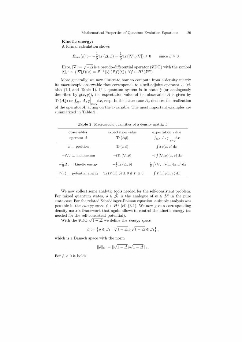
Mathematical Properties of Quantum Evolution Equations 29
Kinetic energy:A formal calculation shows
Ekin(ˆ) := −1
2Tr (∆x ˆ) =
1
2Tr (|∇| ˆ|∇|) ≥ 0 since ˆ≥ 0 .
Here, |∇| =√−∆ is a pseudo-differential operator (ΨDO) with the symbol
|ξ|, i.e. (|∇|f)(x) = F−1(|ξ|(Ff)(ξ)) ∀f ∈ H1(IRn).
More generally, we now illustrate how to compute from a density matrixits macroscopic observable that corresponds to a self-adjoint operator A (cf.also §1.1 and Table 1). If a quantum system is in state ˆ (or analogouslydescribed by (x, y)), the expectation value of the observable A is given by
Tr (A ˆ) or∫
IRN Ax∣∣∣x=y
dx, resp. In the latter case Ax denotes the realization
of the operator A, acting on the x-variable. The most important examples aresummarized in Table 2.
Table 2. Macroscopic quantities of a density matrix ˆ.
observables: expectation value expectation value
operator A Tr (A ˆ)R
IRN Ax˛˛˛x=y
dx
x ... position Tr (x ˆ)Rx(x, x) dx
−i∇x ... momentum −iTr (∇x ˆ) −iR(∇x)(x, x) dx
− 1
2∆x ... kinetic energy − 1
2Tr (∆x ˆ) 1
2
R(∇x · ∇y)(x, x) dx
V (x) ... potential energy Tr (V (x) ˆ) ≥ 0 if V ≥ 0RV (x)(x, x) dx
We now collect some analytic tools needed for the self-consistent problem.For mixed quantum states, ˆ ∈ J1 is the analogue of ψ ∈ L2 in the purestate case. For the related Schrodinger-Poisson equation, a simple analysis waspossible in the energy space ψ ∈ H1 (cf. §3.1). We now give a correspondingdensity matrix framework that again allows to control the kinetic energy (asneeded for the self-consistent potential).
With the ΨDO√
1 −∆ we define the energy space
E :=
ˆ ∈ J1
∣∣√
1 −∆ ˆ√
1 −∆ ∈ J1
,
which is a Banach space with the norm
||| ˆ|||E := |||√
1 −∆ ˆ√
1 −∆|||1 .
For ˆ≥ 0 it holds
30 Anton Arnold
||| ˆ|||E = Tr ((1 −∆)ˆ) = Tr ˆ+ 2Ekin(ˆ) .
In order to estimate the particle density n, and hence the self-consistentpotential V in terms of ˆ (analogously to (18)) we shall need the followingLieb-Thirring-type inequality [LT76, LP93, Arn96]. This is a collective Sobolevor Gagliardo-Nierenberg inequality.
Lemma 4.3 ([Arn96]). Let 1 ≤ p ≤ NN−2 (or 1 ≤ p ≤ ∞ if N = 1; 1 ≤ p <
∞ if N = 2) and θ := N−p(N−2)2p ∈ [0, 1]. Then
‖n[ ˆ]‖Lp(IRN ) ≤ Cp||| ˆ|||θ1 Ekin(| ˆ|)1−θ, ∀ ˆ∈ E
Proof (for N ≥ 3).Consider p = 1, θ = 1 :
‖n‖L1 ≤ ||| ˆ|||1 follows from (23) .
Consider p = p∗ := NN−2 , θ = 0 : Then,
‖n‖Lp∗ ≤∑
j
|λj | ‖ψj‖2L2p∗ ≤ C
∑
j
|λj | ‖∇ψj‖2L2 = 2CEkin(| ˆ|)
follows by the Sobolev inequality. And the general case follows by interpola-tion. ⊓⊔
Remark 4.4. A similar result with ||| ˆ|||θq , q > 1 on r.h.s. was obtained in[LP93]. Its proof is much harder.
4.3 Time Evolution of Closed / Hamiltonian Systems
Assume that the time evolution of a wave function is determined by the Hamil-tonian H , e.g. H(t) = − 1
2∆ + V (t). The Schrodinger equation for a generalpure state then reads
iψt = Hψ, t ∈ IR . (25)
Next we consider the eigenfunction decomposition for :
(x, y, t) =∑
j
λjψj(x, t)ψj(y, t) . (26)
Using (25) in (26) yields the evolution equation for the density matrix. Ifˆ∈ J2 or equivalently (., ., t) ∈ L2(IR2N ), this evolution can be written as aPDE for the kernel (t) (cf. Remark 4.2):
it = (Hx −Hy), t ∈ IR . (27)
Mathematical Properties of Quantum Evolution Equations 31
Here, Hx and Hy denote copies of the Hamiltonian H acting, resp., on the x-and y-variable. This is called the quantum Liouville or von Neumann equation(in coordinate representation).
However, if ˆ∈ J1, its evolution cannot be written as a PDE (cf. Remark4.2). Instead, one has to write it as an abstract evolution problem (Banachspace–ODE) for ˆ(t):
id
dtˆ = [H, ˆ] := H ˆ− ˆH, t ∈ IR . (28)
Also this variant of (27) is called quantum Liouville or von Neumann equation.
In order to solve it, we first consider the free Hamiltonian H0 := − 12∆.
According to (28), the corresponding infinitesimal generator of the C0–groupG0(t), t ∈ IR, for the ˆ–evolution formally reads h0 = −i[H0, ˆ]. G0(t) hasthe following explicit representation:
G0(t)ˆ = e−iH0t ˆeiH0t , t ∈ IR , (29)
with the kernel ∑
j
λj(e−iH0tψj)(x) (eiH0tψj)(y) .
One can see that the density matrix ˆ(t) solving (28) has eigenvalues thatare constant in time. The corresponding eigenvectors obey the Schrodingerequation (25) and stay orthonormal during the evolution (which implies thatthey can only ‘rotate’ in L2(IRN )).
The following lemma gives additional properties of the evolution groupG0(t) and its generator h0:
Lemma 4.5. [DL88a]
(a) G0(t) is a C0–group of isometries on J1 It preserves self-adjointness andpositivity.
(b) Its generator is characterized by
D(h0) = ˆ∈ J1
∣∣ ˆD(H0) ⊂ D(H0), (H0 ˆ− ˆH0) is an operator with
domain H2(IRN ) and it can be extended to L2(IRN ), such that
H0 ˆ− ˆH0 ∈ J1,h0(ˆ) := −i(H0 ˆ− ˆH0) .
Proof (of part (a)). The strong J1–continuity of G0(t) at t = 0 follows fromthe following two ingredients:
|||G0(t)ˆ|||1 = ||| ˆ|||1 since λj = const. in t (convergence of the J1−norm),
〈f, (G0(t)ˆ) g〉 = 〈 eiH0tf︸ ︷︷ ︸
∈C(IR;L2)
, ˆ︸︷︷︸
∈B(L2)
(eiH0tg)〉 t→0−→ 〈f, ˆg〉 ∀f, g ∈ L2
(weak operator convergence).
32 Anton Arnold
These two properties imply the desired J1–convergence. This is a corollary toGrumm’s Theorem (cf. [Sim79]).
The preservation of self-adjointness and positivity follows directly from(29). ⊓⊔
The above result for the evolution in J1 can easily be modified to ananalogous result for the evolution in the energy space E :
Corollary 4.6. h0 generates a C0–group of isometries on E.
Proof. The operators√
1 −∆ and e−iH0t commute. Hence:
√1 −∆ (G0(t)ˆ)
√1 −∆ = e−iH0t (
√1 −∆ ˆ
√1 −∆
︸ ︷︷ ︸
∈J1
) eiH0t ∈ C(IR;J1) .
⊓⊔
4.4 Von Neumann–Poisson Equation in IR3
Here, we present the density matrix analogue of the H1–analysis for aSchrodinger–Poisson system (SPS) (cf. §3.3). The von Neumann–Poissonequation for ˆ(t) discussed here is almost equivalent to the SPS-analysis inH1:Via the SPS-analysis one constructs a corresponding solution ˆ ∈ C(IR; E),hence the existence of a solution is guaranteed. However, its uniqueness in J1
or E would stay open.Since the SPS-analysis is technically much simpler than the density matrix
analysis, a J1–analysis would hence (almost) not be worth the effort for closed,i.e. Hamiltonian systems. However, the time evolution of open quantum sys-tems (cf. §6) cannot be rewritten as a SPS. For such models, the ˆ–analysisseems therefore unavoidable.
We start with the analysis of the repulsive von Neumann–Poisson equa-tion:
i ddt ˆ(t) = [− 12∆+ V (t), ˆ(t)], t ∈ IR
V (t) = 14π|x| ∗ n[ ˆ(t)]
ˆ(0) = σ
(30)
Theorem 4.7. Let σ ∈ E. Then (30) has a unique solution ˆ ∈ C(IR; E). Itsatisfies ||| ˆ(t)|||1 = |||σ|||1.
Proof. Morally, we follow the proof of Theorem 3.2. But since we are dealingwith the evolution of operators instead of functions, we have to cope withmany technical difficulties (Lieb-Thirring-type inequality instead of Sobolevinequality, e.g.):
1. G0(t) is a C0–group of isometries on J1, J1, E (see Sect. 4.3).2. f(ˆ) := −i[V [ ˆ], ˆ] is locally Lipschitz in E (but not in J1):
Mathematical Properties of Quantum Evolution Equations 33
• ˆ∈ E ⇒ V [ ˆ] ∈ L∞(IR3) by (18) and the Lieb-Thirring-type inequal-ity from Lemma 4.3.
• We need to show that√
1 −∆ (V ˆ)√
1 −∆ ∈ J1:(i) First we decompose the ΨDO
√1 −∆ as follows:
√1 −∆ = 1 +
∑
j
Kj︸︷︷︸
∈B(L2)
∂xj.
This allows to use the product rule for (V ˆ). Here, Kj is a ΨDOwith the symbol
iξj|ξ|2 (
√
1 + |ξ|2 − 1)
(ii) Next we need to show that V ˆ√
1 −∆, ∇(V ˆ√
1 −∆) ∈ J1 . Forthe first term we use that
√1 −∆ ˆ
√1 −∆ ∈ J1
ˆ≥0=⇒ ˆ
1
2
√1 −∆, ˆ
1
2 ∈ J2 .
For simplicity we assumed here first that ˆ ≥ 0 (but it can begeneralized). Next, the “Holder inequality” for the operator spacesJp (cf. [RS75]) yields
V︸︷︷︸
∈B
ˆ1
2
︸︷︷︸
∈J2
(ˆ1
2
√1 −∆
︸ ︷︷ ︸
∈J2
) ∈ J1 .
3. Prop. 3.1 yields: The von Neumann–Poisson equation (30) has a uniquelocal solution ˆ∈ C([0, tmax); E).
4. We have the a-priori estimates ||| ˆ(t)|||1 = const in t, Ekin(ˆ(t)) is uniformlybounded (in t). Hence, the solution is global on IR.
⊓⊔
Remark 4.8. The quantum attractive case (with V (t) = − 14π|x| ∗n[ ˆ(t)]) can
be included with the following estimate (using the Lieb-Thirring-type inequal-ity):
−Epot(ˆ) := ‖∇V ‖2L2 ≤ C‖n‖2
6
5
≤ C||| ˆ|||3
2
1 Ekin(ˆ)1
2
(cf. [Arn96]). A similar strategy also works for SP-analysis in §3.
5 Wigner Function Models
5.1 Wigner Functions
A Wigner function is obtained from the corresponding density matrix functionby the Wigner-Weyl transformation (cf. [W32, SS87]):
34 Anton Arnold
w(x, v, t) = (2π)−N/2Fη→v
(
x+hη
2m,x− hη
2m, t
)
= (2π)−N∑
j
λj
∫
IRN
ψj(x+hη
2m, t)ψj(x− hη
2m, t)e−iv·η dη .
Since (x, y) = (y, x), we have w(x, v) ∈ IR. Moreover,
w ∈ L2(IR2N ) ⇔ ∈ L2(IR2N ) ⇔ ˆ∈ J2(L2(IRN)) .
We call w a physical Wigner function, if it corresponds to a density matrix0 ≤ ˆ∈ J1.Following [SS87] we now also give the direct transformation from the densitymatrix operator ˆ to the Wigner function w: With the Weyl operators
W (ξ, η) := e−i(ξ·x−ihmη·∇x), for each ξ, η ∈ IRN
we have
w(x, v, t) = (2π)−2N
∫∫
IR2N
Tr(ˆ(t)W (ξ, η)
)ei(ξ·x+η·v) dξdη .
Since the operators ξ · x − i hmη · ∇x are essentially self-adjoint on C∞0 (IRN )
∀ ξ, η ∈ IRN (cf. Lemma 5.3, Example 5.4, below), W (ξ, η) is a unitary oper-ator on L2(IRN ) by Stone’s Theorem (cf. [Paz83]). Hence, Tr
(ˆ(t)W (ξ, η)
)is
well-defined for ˆ∈ J1 and each ξ, η ∈ IRN .The time evolution of w follows from the von Neumann equation: The
Wigner equation reads
wt + v · ∇xw − eΘ[V ]w = 0, x, v ∈ IRN , t ∈ IR , (31)
with the pseudo-differential operator (ΨDO)
Θ[V ]w(x, v)
=i
h(2π)−N
∫∫
IR2N
[
V (x+hη
2m) − V (x− hη
2m)
]
w(x, v)ei(v−v)·η dvdη .
In the classical limit, Θ[V ] converges formally to its classical counterpart(see [LP93] for rigorous results). For a fixed function w = w(x, v) and a fixedpotential V = V (x), we have:
Θ[V ]wh→0−→ 1
m∇xV · ∇vw .
For a quadratic potential V , the operator Θ[V ] takes exactly the form of itsclassical counterpart:
Θ[V ]w =1
m∇xV · ∇vw . (32)
Mathematical Properties of Quantum Evolution Equations 35
In this special case the Wigner equation (formally) looks like the classicalLiouville equation
ft + v · ∇xf − e
m∇xV · ∇vf = 0, x, v ∈ IRN . (33)
Note that the Liouville equation and also the nonlinear Liouville-Poissonequation (also called Vlasov-Poisson equation) preserve all Lp–norms in time,i.e.
‖f(., ., t)‖Lp(IR2N ) = const. in t ∀1 ≤ p ≤ ∞, t ∈ IR .
This is implied by the fact that the solution of (33) is constant along itscharacteristics. In contrast, the Wigner equation (in general) only preservesthe L2(IR2N )–norm, since v · ∇x − eΘ[V ] is skew-adjoint.
If V ∈ L∞(IRN ), then ‖Θ[V ]‖B(L2) ≤ 2h‖V ‖L∞ . Hence, in this case there
exists a C0–evolution group of isometries for the Wigner equation on L2(IR2N ).This follows from Stone’s theorem. Moreover, Θ[V ] is a bounded perturbationof v · ∇x .
From now on we set the parameters e = m = h = 1 and we recall thedefinition of the macroscopic quantities for a Wigner function w:
• typical normalization of total mass:∫∫
IR2N w dxdv = 1• particle density: n(x, t) :=
∫
IRN w(x, v, t) dv (≥ 0 for a physical Wignerfunction)
• current density: j(x, t) :=∫
IRN vw(x, v, t) dv
• kinetic energy density: ekin(x, t) :=∫
IRN
|v|2
2 w(x, v, t) dv (≥ 0 for a physicalWigner function)
Note that these definitions are purely formal since a Wigner function satisfiesw(., ., t) ∈ L2(IR2N ) but typically w 6∈ L1(IR2N ). Hence, the “definition”n := “
∫w dv ” is meaningless !
This is a key problem for analyzing the self-consistent Wigner-Poissonequation, i.e. (31) with the Coulomb potential obtained from −∆V = n =∫w dv. In other words, the quadratically nonlinear term Θ[V [w]]w is not
defined pointwise in t on the state space of the Wigner function (w(t) ∈ L2,e.g.). This is the same problem like in the L2–analysis of SP in §3.2. Thereare two simple solutions to this problem:
• Change the state space for w (even if it is not very physical): A weightedL2–space with sufficient weight in the v-variable implies w ∈ L2
x(L1v) and
hence n ∈ L2(IRNx ). Possible options are:in 1D: w ∈ L2(IR2; (1 + v2) dxdv), cf. [ACD02]in 3D: w ∈ L2(IR6; (1 + |v|4) dxdv), cf. [ADM07]
• For Hamiltonian or closed systems (i.e. without collision operators in theWigner equation) the Wigner-Poisson equation is (almost) equivalent tothe SPS (§3.3). This allows for a much simpler analysis (cf. Theorem 3.5(a),and [BM91, AN91, ILZ94, MRS90]).
36 Anton Arnold
5.2 Linear Wigner-Fokker-Planck: Well-posedness
We shall now consider an open quantum system that includes a collision oper-ator on the r.h.s. of (31). Such a model is not any more equivalent to a systemof Schrodinger equations. Any mathematical analysis must hence be done onthe level of Wigner functions or density matrices. In this and the next sectionwe shall illustrate both approaches.
In this subsection and in §5.3 we analyze the linear Wigner-Fokker-Planckequation (WFP) with an external potential of the form µ
2 |x|2 + V (x), µ ∈IR, V ∈ L∞(IRN). Because of (32), the quadratic potential yields the classicalpotential term. Hence, the WFP equation reads:
wt + v · ∇xw − µx · ∇vw − Θ[V ]w = Qw , x, v ∈ IRN , t > 0Qw = Dpp∆vw
︸ ︷︷ ︸
class. diffusion
+ 2γ divv(vw)︸ ︷︷ ︸
friction
+Dqq∆xw + 2Dpq divx(∇vw)︸ ︷︷ ︸
quantum diffusion
w(x, v, t = 0) = w0(x, v)
(34)
• This model is quantum mechanically “correct” if the following Lindbladcondition holds:
DppDqq −D2pq ≥
γ2
4. (35)
Exactly in this case, (34) can be rewritten as a Lindblad equation (see (50)below) for the corresponding density matrix operator [ALMS04, SS87]. Asa consequence, the positivity of the particle density is preserved under thetime evolution: n(x, t) ≥ 0, ∀x, t. Note that the “classical Fokker-Planck-term”, i.e. the so-called Caldeira-Leggett model [CL83], with Dqq = Dpq =0 does not satisfy the Lindblad condition (35). Nevertheless it is frequentlyused in applications, yielding reasonable results.
• The collision operator Qw models diffusive effects (e.g. the electron-phonon-interaction). Hence, (34) has applications for the electron trans-port in quantum semiconductors and for quantum Brownian motion.
• A derivation of (34) from the coupling of electrons to a bath of harmonicoscillators was given in [CEFM00].
Next we give an existence result for the linear WFP equation (34). Thefollowing theorem crucially depends on the Lumer-Phillips Theorem (cf.[Paz83]):
Proposition 5.1. Let the operator A be densely defined and closed on the Ba-nach space X. Let A and A∗ be dissipative. Then, A generates a C0–semigroupof contractions on X.
We rewrite (34) as an evolution problem on L2(IR2N ):
wt = Aw +Θ[V ]w, t > 0 ,
w(0) = w0 ∈ L2(IR2N ) ,(36)
Mathematical Properties of Quantum Evolution Equations 37
with the abbreviation
Aw := −v · ∇xw + µx · ∇vw +Qw
= −v · ∇xw + µx · ∇vw + 2γ divv(vw)
+ Dpp∆vw + 2Dpq divv(∇xw) +Dqq∆xw .
Theorem 5.2. Let V ∈ L∞(IRN ) or V ∈ L1loc
(IR+;L∞(IRN )
). Then (36)
has a unique mild solution w ∈ C([0,∞);L2(IR2N )
).
Proof.
• We define the operator A := A−Nγ on the domain D(A
):= C∞
0
(IR2N
).
• Then, A is dissipative on D(A
)and A∗ is (formally) dissipative in
L2(IR2N ), i.e. 〈Aw,w〉L2 ≤ 0 ∀w ∈ D(A
). The rigorous proof of dis-
sipativity for A∗ will follow from Lemma 5.3 below.
• From the Lumer-Phillips Theorem then follows: ¯A generates a C0-semigroup:∥∥∥etAw
∥∥∥L2
≤ eNγt ‖w‖L2 , t ≥ 0 . (37)
• The final result follows, since Θ[V ] is a bounded perturbation on L2(IR2N )(see Prop. 2.7 or 3.1, resp.).
⊓⊔Now we still have to prove the dissipativity of A∗ on D(A∗). Just like for
A, one immediately finds that A∗|D(A) is dissipative, with
A∗ = v·∇xw−µx·∇vw−2γ v·∇vw+Dpp∆vw+2Dpq divv(∇xw)+Dqq∆xw−Nγ .
However, D(A∗) is not known explicitly. To verify that A∗ is the closure ofA∗|D(A) we shall use the following lemma, since A∗ is a quadratic polynomialin x, v, ∇x, ∇v:
Lemma 5.3 ([ACD02], [AS04]). Let the operator P = p2(x,−i∇) be aquadratic polynomial in x, −i∇. Define the minimum realization of P on
D (Pmin) := C∞0
(IRN
)⊆ L2
(IRN
).
Then, Pmin = Pmax, the maximum extension of P, i.e.
D (Pmax) =f ∈ L2|Pf ∈ L2
.
Proof. For f ∈ D(Pmax) we need to show, that it can be approximated in thegraph norm ‖.‖P by a sequence fn ⊂ C∞
0
(IRN
). This is accomplished by
the following (standard) approximation sequence (but the proof is lengthy):
fn(x) := χn(x)︸ ︷︷ ︸
C∞0
-cutoff
· (f ∗ ϕn︸︷︷︸
C∞0
-mollifier
)(x)n→∞−→ f in ‖.‖P .
⊓⊔
38 Anton Arnold
The following examples illustrate applications and limitations of thislemma:
Example 5.4. We consider several Schrodinger operators. Their essential self-adjointness on C∞
0 (IRN ) is crucial for the existence of a corresponding evolu-tion group (cf. [RS75]).
(a) P = −∆− |x|2, D(P ) = C∞0 (IRN ) is essentially self-adjoint in L2(IRN ).
(b) P = −∂2x + x4, D(P ) = C∞
0 (IR) is also essentially self-adjoint in L2(IR)[RS75]. Hence, Lemma 5.3 can be extended to this case of a positivequartic potential.
(c) P = −∂2x − x4, D(P ) = C∞
0 (IR) is not essentially self-adjoint in L2(IR)[RS75]. Hence, Lemma 5.3 cannot be extended to this negative quarticpotential. Note, that for this potential (classical) particles would run offto x = ∞ in finite time. Hence, no reversible, mass conserving dynamicscan exist.
So we conclude, that Lemma 5.3 cannot be extended to all operators of theform P = p4(x,−i∇) (i.e. quartic polynomials) — neither to all cubic poly-nomials, by the way.
5.3 Linear Wigner-Fokker-Planck: Large Time Behavior
First we consider the case of a quadratic external confinement potentialV (x) = µ
2 |x|2, µ ≥ 0. Because of (32), the linear Wigner-Fokker-Planckequation (WFP) then takes the form of a classical kinetic equation:
wt + v · ∇xw − µx · ∇vw = Qw , x, v ∈ IRN , t > 0
Qw := Dpp∆vw + 2γ divv(vw) +Dqq∆xw + 2Dpq divx(∇vw)
w(x, v, t = 0) = w0(x, v)w(x, v, t = 0) = w0(x, v) ∈ L2(IR2N )
(38)
Theorem 5.5 ([SCDM04]).
(a) (38) has a Green’s function G(x, v, x0, v0, t) ≥ 0 (it is a non-isotropicGaussian).
(b) ∃! mild (and actually classical) solution of (38):
w(x, v, t)=
∫∫
G(x, v, x0, v0, t)w0(x0, v0) dx0 dv0 ∈ C([0,∞);L2(IR2N )) .
(39)When transforming (x, v) to the characteristic coordinates of the Liouvilleequation wt + v · ∇xw − µx · ∇vw = 0, the integral in (39) becomes aconvolution in x0, v0.
(c) w0(x, v) ≥ 0 ⇒ w(x, v, t) ≥ 0 ∀t ≥ 0 .
The dissipativity introduced by the collision operator Q and the confine-ment of the potential V makes the system converge to the equilibrium. Thissteady state w∞ is unique up to the normalization of mass:
Mathematical Properties of Quantum Evolution Equations 39
Theorem 5.6 ([SCDM04]). Let γ > 0 and µ > 0. Then
(a) The WFP equation (38) has a unique steady state (up to normalizationof mass):
w∞(x, v) = e−[α|x|2+2βx·v+γ|v|2] .
It is a non-isotropic 2N -dimensional Gaussian.
(b) w(t)t→∞−→ w∞(x, v) in relative entropy (cf. (52)), L1(IR2N ), and in
L2(IR2N ) with an exponential rate. Here, w∞ is normalized as
∫ ∫
w∞dxdv =
∫ ∫
w0dxdv .
Proof (of (b)).This is an application of the entropy method (cf. [AMTU01]) for uniformlyparabolic drift-diffusion equations with a uniformly convex “potential”. Themethod is applied separately for the positive and negative part of the Wignerfunction: w±(x, v, t). ⊓⊔
Remark 5.7. In contrast to classical kinetic models, w∞ does not separatelyannihilate the collision term Qw and the transport term v · ∇xw − µx · ∇vwin (38). This reflects the non-local flavor of quantum mechanics.
Next we present a recent extension of Theorem 5.6 for (small) perturba-tions λV0 of the harmonic oscillator potential (cf. [AGGS07]). We considerthe linear WFP equation (36) with the identity as diffusion matrix (just fornotational simplicity):
wt = Aw + λΘ[V0]w, t > 0 ,w(0) = w0,
(40)
with the abbreviation
Aw := −v · ∇xw + x · ∇vw +Qw
= −v · ∇xw + x · ∇vw + 2 divv(vw) +∆vw +∆xw .
Let w∞(x, v) > 0 denote the unperturbed steady state (i.e. for λ = 0) fromTheorem 5.6. It is unique when imposing the normalization
∫∫
IR2N w∞ dxdv =
1. We introduce the weighted Hilbert space H := L2(IR2N , w−1∞ dxdv).
Then we have
Theorem 5.8 ([AGGS07]). Let V0 ∈ C∞(IRN ), such that V0 decays suf-ficiently fast (see [AGGS07] for the details), and let |λ| > 0 be sufficientlysmall. Then
(a) the WFP equation (40) has a unique steady state w∞ ∈ H, satisfying thenormalization condition
∫∫
IR2N w∞ dxdv = 1.
40 Anton Arnold
(b) For any initial function w0 ∈ H with∫∫
IR2N w0 dxdv = 1 we have expo-nential convergence towards the steady state:
‖w(t) − w∞‖H ≤ e−εt‖w0 − w∞‖H, t ≥ 0,
with some ε > 0.
Proof.
(a) We rewrite the stationary version of (40) as the fixed point problem
Aw = −λΘ[V0]w
in order to use Banach’s fixed point theorem. Since A has a non-trivialkernel (in fact Aw∞ = 0 by Theorem 5.6), we cannot invert A. Hence wedefine H⊥ := f ∈ H : f⊥w∞ and modify the fixed point problem to
Az = −λΘ[V0](z + w∞) (41)
for z := w − w∞ ∈ H⊥. Now, λA−1Θ[V0] is contractive on H⊥ and itsunique fixed point z∗ yields the unique normalized steady state w∞ =z∗ + w∞ ∈ H of (40).
(b) Consider on H⊥ the evolution of v(t) := w(t) − w∞, with w(t) satisfying(40). Then, ‖v(t)‖2
H is a Lyapunov functional with exponential decay:For computing d
dt‖v(t)‖2H we use that the operator A has a spectral gap
of size σ = 1− 1/√
2 on H. Hence, its symmetric part As satisfies on H⊥:As ≤ −σ. The idea is now that the perturbation potential λΘ[V0] can becompensated by this spectral gap. ⊓⊔
5.4 Wigner-Poisson-Fokker-Planck: Global Solutions in IR3
The Wigner-Poisson-Fokker-Planck (WPFP) system reads:
wt + v · ∇xw −Θ[V ]w = Qw, x, v ∈ IR3, t > 0Qw = Dpp∆vw
︸ ︷︷ ︸
class. diffusion
+ 2γ divv(vw)︸ ︷︷ ︸
friction
+Dqq∆xw + 2Dpq divx(∇vw)︸ ︷︷ ︸
quantum diffusion
−∆V (x, t) = n(x, t) :=∫w(x, v, t) dv
w(x, v, t = 0) = w0(x, v)
(42)
This is an open quantum systems with mean-field potential. For proving theexistence of a global-in-time solution to (42) we face two analytical problems:
1. For w ∈ L2(IR6) the nonlinear potential term is not locally Lipschitz. Thismakes the construction of a local-in-time solution difficult. Actually, theparticle density n(x, t) is not defined pointwise in time.
Mathematical Properties of Quantum Evolution Equations 41
2. We lack enough (physical) a-priori estimates to establish a global-in-tsolution.
First we discuss the difficulties with the a-priori estimates: For WPFP, theonly simple a-priori estimate is (cf. (37))
‖w(t)‖2 ≤ e3γt‖w0‖2, t≥0,
which follows from the skew-adjointness of v · ∇x − Θ[V ]. But we have noother Lp–estimates.The physical conservation laws (like mass conservation
∫∫w(x, v, t) dxdv =
const, or an energy balance involving the total kinetic energy Ekin(t) =12
∫ ∫|v|2w(x, v, t) dxdv, cf. [ALMS04]) are not usable here, since w ∈ IR
(unless ˆ(t) ≥ 0 is used, as in [CLN04]).
The main idea for tackling both of the above problems is to find a newa-priori estimate for the electric field E = E(x, t) in the WPFP equation.This will be used both
• for the construction of the local-in-time solution via a fixed point map,and
• to establish the global-in-time solution.
Since the particle density n[w] =∫w dv cannot be rigorously defined point-
wise in t, we shall somehow eliminate it from the WPFP system. Instead, weshall define the electric field E = −∇V = 1
4πx
|x|3 ∗∫w dv a.e. in t using the
dispersive regularization of the free transport equation wt + v · ∇xw = 0.
A-priori estimate for electric field in Wigner-Poisson:
We proceed similarly to [Per96] for the Vlasov-Poisson (VP) system, or[Cas98] for the Vlasov-Poisson-Fokker-Planck system.
To keep the notation simple we first illustrate the strategy for the Wigner-Poisson system, which reads in Duhamel form:
w(x, v, t) = w0(x − vt, v) −∫ t
0
(Θ[V ]w)(x−vs, v, t−s) ds . (43)
Using the particle density n =∫w dv from (43) we split the field as E(x, t) =
−∇V (x, t) = 14π
x|x|3 ∗ n(x, t) = E0 + E1:
E0(x, t) :=1
4π
x
|x|3 ∗x∫
w0(x−vt, v) dv ,
E1(x, t) := − 1
4π
x
|x|3 ∗x∫ t
0
∫
IR3v
(Θ[V ]w)(x−vs, v, t−s) dv ds . (44)
For VP (studied in [Per96]) the corresponding term has the form
42 Anton Arnold
E1(x, t) = − 1
4π
x
|x|3 ∗x∫ t
0
∫
(∇xV · ∇vw)(x−vs, v, t−s) dv ds
= − 1
4π
x
|x|3 ∗x divx
∫ t
0
s
∫
(∇xV w)(x−vs, v, t−s) dv ds . (45)
Here, the key issue is that the second factor of this last convolution is in diver-gence form, in order to pass that divx to the first convolution factor later on.Obviously, this is not the case in (44). However, with a tricky reformulation,Θ[V ] can indeed be written in divergence form:
Θ[V ]w = F−1η→v (δV (x, η)w(x, η)) = ∇xV ∗x Φ(x, v) ∗v ∇vw,
with some distribution Φ(x, v) and
δV (x, η) = V (x+η
2) − V (x− η
2) =
∫ 1
2
− 1
2
η · ∇xV (x−rη) dr .
We illustrate this computation for the (simpler) 1D case:
δV (x, η)w(x, η) = η∇xV ∗x(
1
|η|χ[−|η|/2,|η|/2]
)
(x)
︸ ︷︷ ︸
=:Φ(x,η)
w(x, η) .
Following the strategy from (45), we can rewrite the components j = 1, 2, 3of the field E1 as
(E1)j(x, t)=1
4π
3∑
k=1
3xjxk − δjk|x|2|x|5 ∗x
∫ t
0
s
∫
(∂xkV ∗xΦ∗vw)(x−vs, v, t−s) dv ds .
This yields the following a-priori estimate for the WP case on any timeinterval (0, T ) [ADM07]:
Lemma 5.9. Let w0∈L2(IR6) and∥∥∫w0(x − vt, v) dv
∥∥Lq
x(IR3)≤ t−ωq , t ≤ T .
Then, it holds for 0 < t ≤ T :
‖E1(t)‖L2(IR3) ≤ C
∫ t
0
s ds
∥∥∥∥
∫
(∇V ∗x Φ ∗v w)(x−vs, v, t−s) dv
∥∥∥∥L2
x(IR3)
≤ C
∫ t
0
s ds
s3/2‖(E0 + E1)(t−s)‖L2(IR3) ‖w0‖L2(IR6) .
Hence,
‖E0(t)‖L2(IR3) + ‖E(t)‖L2(IR3) ≤ Ct−3
2q+ 5
4−ωq .
This lemma only provides an L2–estimate on E(t) for the WP system. Forthe VP system, however, one obtains a whole interval of Lp–estimates. Thisis due to the conservation of all norms ‖f(t)‖Lp(IR6), 1 ≤ p ≤ ∞ in the VP
Mathematical Properties of Quantum Evolution Equations 43
case, while WP only conserves the L2–norm in time.
A-priori estimate for electric field in WPFP:
The WPFP system reads
wt = Aw +Θ[V ]w ,
−∆V (x, t) = n(x, t) :=
∫
w(x, v, t) dv ,
with the abbreviation
Aw := −v∇xw + 2γ divv(vw) +Dpp∆vw +Dqq∆xw + 2Dpq divx(∇vw) .
Using the Green’s function G(x, v, x0, v0, t) from Theorem 5.5, the WPFPsolution can be written in Duhamel form:
w(x, v, t) =
∫ ∫
IR6
G(x, x, x0, v0, t)w0(x0, v0) dx0 dv0
−∫ t
0
∫ ∫
IR6
G(x, x, x0, v0, s)(Θ[V ]w)(x0, v0, t−s) dx0 dv0 ds .
Proceeding like for the WP case, we obtain an a-priori estimate on thefield for the WPFP system [ADM07]:
Lemma 5.10. Let w0 ∈ L2 and∥∥∫w0(x−vt, v) dv
∥∥Lq
x≤ t−ωq , t ≤ T . Then,
it holds for 0 < t ≤ T :
‖E0(t)‖p + ‖E(t)‖p ≤ Ct3
2p− 3
2q+ 1
2−ωq , 2 ≤ p < 6 .
For p > 2, this result is obtained by the parabolic regularization ofG(t). Hence, this result goes beyond the WP-result in Lemma 5.9. For theiterative construction of the local-in-time solution we shall need in fact:E ∈ L1((0, T ), L3(IR3)). Hence, our procedure works for WPFP but not (yet)for WP.
Next we illustrate that the assumptions on w0 in Lemma 5.9, 5.10 can beobtained quite naturally. With theNotation:
L1x(L
qv) := L1(IR3
x;Lq(IR3
v)), 1 ≤ q ≤ ∞we use the Strichartz estimate for the free transport equation [CP96]:
∥∥∥∥
∫
w0(x−vt, v) dv∥∥∥∥Lq
x(IR3)
≤ C |t|−3(1− 1
q) ‖w0‖L1
x(Lqv) , t ∈ IR . (46)
Hence, w0 ∈ L1x(L
qv) yields exactly the needed assumption. When choosing
some q ∈[1, 6
5
), (46) and Lemma 5.10 imply ‖E(t)‖3 ∈ L1(0, T ), as needed.
44 Anton Arnold
Once we have an a-priori estimate for the field E on any (0, T ], we candefine the potential V using the Poisson equation divE = n:
V =1
4π|x| ∗ n =1
4π|x| ∗ divE = − 1
4π
∑
j
xj|x|3 ∗ Ej , (47)
and analogously for the “split quantities” V0, V1, n0, n1 (cf. (44) for the split-ting of E). This implies the following a-priori estimate on the self-consistentpotential V :
Lemma 5.11. Let w0 ∈ L2and∥∥∫w0(x−vt, v) dv
∥∥Lq
x≤ t−ωq , t ≤ T .
Then, it holds for 0 < t ≤ T :
‖V (t)‖p ≤ Ct3
2p− 3
2q+1−ωq , 6 ≤ p ≤ ∞ ,
and henceΘ[V (t)] ∈ B(L2(IR6)), t > 0 .
Definition of the nonlinear term Θ[V [w]]w:
The standard definition of the macroscopic quantities: density, self-consistentpotential, and self-consistent field are made pointwise in time:
n(x, t) =
∫
w(x, v, t) dv, V (x, t) =1
4π|x| ∗x n(x, t), E(x, t) = −∇xV (x, t) .
However, this is unfeasible for w ∈ L2.Therefore, we shall use the following alternative definition, which is nonlo-
cal in t, via an integral equation for E1. This is based on the above derivationof the a-priori estimate for E1, and it yields a nonlinear map w 7→ E1[w]. Wepresent it here for the WP case (to keep the notation simple), but the WPFPcase is analogous:
E1[w]j(x, t) (48)
= − 1
4π
3∑
k=1
3xjxk − δjk|x|2|x|5 ∗x
∫ t
0
s
∫
(E[w]k ∗x Φ ∗v w)(x−vs, v, t−s) dv ds .
Using (47) we then obtain (the inhomogeneous parts of) the potential anddensity:
V1[w] = − 1
4π
∑
j
xj|x|3 ∗ E1[w]j , n1[w] = −∆V1[w] . (49)
Note that the a-priori estimate on E1[w] only depends on w0 and ‖w(t)‖2
(cf. Lemma 5.9, 5.10). Hence, E1[w] ∈ L1((0, T );L2(IR3)) is well-defined from
Mathematical Properties of Quantum Evolution Equations 45
(48) for all Wigner trajectories w ∈ C([0, T ];L2(IR6)). For this definition w(t)need not be the self-consistent Wigner function solving WPFP.
While the two above definitions of E = E0 +E1 will generally be different,they coincide for the self-consistent solution w.
Iterative construction of the WPFP solution:
For any time interval [0, T ] we now construct the WPFP solution by aniteration map M , defined on the following ball in a Banach space:
BR =w ∈ C([0, T ];L2(IR6))
∣∣ ‖w(t)‖L2 ≤ R
,
with R := e3γT ‖w0‖2 reflecting the exponential growth of the L2–norm:‖w(t)‖2 ≤ e3γt ‖w0‖2.
In the (nonlinear) map M we first associate to w a potential V [w] by (48),(49). Then, w is the solution of the linear WFP (by Theorem 5.2):
wt = Aw +Θ[V [w]]w, t ∈ (0, T ] ,
w(t=0) = w0 .
Summarizing we have
w 7−→ V [w] = V0 + V1[w]︸ ︷︷ ︸
∈L1((0,T );L∞(IR3))
7−→Mw := w .
Lemma 5.12. Let w0 ∈ L2 and∥∥∫w0(x−vt, v) dv
∥∥Lq
x≤ t−ωq , t ≤ T
Then, Mn is a contraction on BR for n = n(T ) large enough.
This lemma implies that the WPFP system has a unique global-in-timesolution:
Theorem 5.13 ([ADM07a]). Let w0 ∈ L2x,v ∩L1
x (Lqv) for some 1 ≤ q < 65 .
Then, WPFP has a unique mild solution:
w ∈ C([0,∞);L2(IR6)) ∩ C((0,∞);C∞B (IR6)) ,
n, V, E ∈ C((0,∞);C∞B (IR3)) .
Proof. For the existence of the mild solution combine Lemma 5.12 and (46).The regularity of w, n, V, E follows a-posteriori by using the regularizationof the WPFP–Green’s function. ⊓⊔
For other analytical approaches for the WPFP system we refer to [ALMS04,CLN04].
46 Anton Arnold
6 Open Quantum Systems in Lindblad Form
In a closed quantum system only interactions within that system exist. Foran open quantum system, however, there actually exist two coupled systems:Firstly, our (finite) quantum system of interest, labeled S. And secondly, thereexists a large reservoir (or “environment”), labeled R. If these two systemsonly interact with each other (but with no other external system), the coupledsystem S +R forms a closed quantum system.
The idea of an open quantum system is now to model only the evolutionof the small quantum system S: One includes the uni-directional interactionof R onto S, but one disregards the influence of S onto R. This is a reasonableapproximation, if R is much larger than S. Henceforth we shall assume thatR is in thermodynamic equilibrium (a “heat bath”) that does not undergoa time evolution while interacting with S. As an example motivated by thediscussion of §1.2, S might model an ensemble of electrons in a semiconductorcrystal, while R models a phonon bath. For a general introduction to openquantum systems we refer to [AF01, AJP06, Dav76].
For the description of an open quantum system and its dynamics we makethe following postulates:
• The open system S at time t is described by a density matrix ˆ(t) ∈ J1(H)with some Hilbert space H.
• The dynamics of S is Markovian (i.e. there are no memory effects) and itis described by a conservative quantum dynamical semigroup (QDS) onJ1(H) (see below).
Definition 6.1. Let G(t), t ≥ 0 be a C0–semigroup on some Hilbert spaceH. Its dual map G(t)∗ on B(H) is called completely positive, if the tensorproduct
G(t)∗ ⊗ In defined on B(H) ⊗ B(Hn)
is positivity preserving ∀n ∈ IN (i.e. it maps positive operators to positiveoperators). Here, Hn denotes any n-dimensional Hilbert space, and In then-dimensional unit matrix.
Definition 6.2. Let G(t), t ≥ 0 be a C0–semigroup on J1(H), with someHilbert space H. G(t) is called a conservative quantum dynamical semigroup,if
• G(t) is trace preserving, i.e. Trˆ(t) = Trˆ(0), t ≥ 0.• G(t)∗ is completely positive.
Remark 6.3. Complete positivity is clearly stronger than the positivity preser-vation. Moreover it is invariant under forming tensor products. This is im-portant, if one wants to recover the dynamics of the coupled system S + Rfrom the dynamics of the open quantum system S.
Mathematical Properties of Quantum Evolution Equations 47
6.1 Lindblad Form
Theorem 6.4 (structure of QDS-generators, [Lin76]). Let L be thebounded generator of a QDS on J1(H). Then, L is in Lindblad form:
L(ˆ) = −i[H, ˆ] +∑
k
(
Lk ˆL∗k −
1
2(L∗
kLk ˆ+ ˆL∗kLk)
)
,
with some Hamiltonian H ∈ B(H) and (maybe countably many) Lindbladoperators Lk ∈ B(H).
Remark 6.5. The boundedness of L is important for the proof of Theorem6.4. The extension of this result to arbitrary unbounded generators L is un-known. Nevertheless, this Lindblad structure of a QDS-generator is a usefuland generally accepted assumption – also for the unbounded case!
The most general type of a Markovian master equation describing theevolution of an open quantum system is the following von Neumann equation(also called Lindblad equation or master equation in Lindblad form):
d
dtˆ = L(ˆ)
= −i[H, ˆ] +∑
k
(
Lk ˆL∗k −
1
2(L∗
kLk ˆ+ ˆL∗kLk)
)
︸ ︷︷ ︸
=:A(ˆ)
. (50)
Here, the operators H, Lk may be unbounded. As we shall see, the evolutionof the density matrix ˆ(t) is now in general non-unitary.
We recall that at each t fixed, ˆ(t) admits a spectral decomposition
ˆ(t) =∑
j∈IN
λj(t) |ψj(t)〉 〈ψj(t)| ,
where ψj(t) are its eigenvectors and λj(t) the eigenvalues. Here, |ψj〉 〈ψj | de-notes the projection operator onto the j-th eigenspace of ˆ(t). In contrast toa closed quantum system (cf. §4.3), the eigenvalues λj(t) are not constant intime in the open quantum system (50). Hence, (50) cannot be reformulatedas a Schrodinger system (cp. to §3.3, 4.3).Moreover the dynamics is not time reversible, since the generator L is dissi-pative:
Definition 6.6. The operator A is called dissipative
(a) on a Hilbert H, if
ℜ〈Ax, x〉 ≤ 0 ∀x ∈ D(A) ⊂ H ;
48 Anton Arnold
(b) on the Banach space J1(H), if
ℜTr(A(ˆ)sgn(ˆ)||| ˆ|||1
)≤ 0 ∀ ˆ∈ D(A) ⊂ J1(H) .
Here, sgn(ˆ) is defined by the functional calculus.
Lemma 6.7. A solution ˆ(t) of (50) formally satisfies:
(a) trace preservation;(b) positivity preservation, i.e. ˆ(0) ≥ 0 ⇒ ˆ(t) ≥ 0 ∀t ≥ 0 ;(c) The generator L is dissipative in J1(H) .
Proof (purely formal, since L might not generate an evolution semigroup).
(a) From (50) it follows ddtTr ˆ(t) = 0 , from the cyclic property of the trace.
(b) Let ˆ≥ 0, and decompose L as:
L1(ˆ) :=∑
k
Lk ˆL∗k ≥ 0 ,
L2(ˆ) := −(H ˆ+ ˆH∗), H := iH +1
2
∑
k
L∗kLk .
Then, ˆ ≥ 0 and ddt ˆ = L1(ˆ) ≥ 0 imply etL1 ˆ ≥ 0, ∀t ≥ 0. Moreover, L2
generates the evolution semigroup
etL2 ˆ = e−tH ˆe−tH∗
,
which preserves positivity. Now we conclude the positivity preservation ofetL by Trotter’s product formula:
etL = limn→∞
[
etnL1e
tnL2
]n
.
(c) In the proof we split the Hamiltonian part from the Lindblad part A(ˆ):
Tr ([H, ˆ] sgn(ˆ)) = Tr (H | ˆ| − | ˆ|H) = 0 ;
ℜTr (Lk ˆL∗k sgn(ˆ) − Lk| ˆ|L∗
k)
= Tr (L∗ksgn(ˆ)Lk ˆ− L∗
kLk| ˆ|)=
∑
j
〈Lkψj , (sgn(ˆ)Lk ˆ− Lk| ˆ|)ψj〉
=∑
j
λj 〈Lkψj , sgn(ˆ)Lk ψj〉︸ ︷︷ ︸
≤‖Lkψj‖2
L2
−∑
j
|λj | ‖Lkψj‖2L2 ≤ 0 ,
with (ψj , λj) denoting the eigenpairs of ˆ. ⊓⊔
Mathematical Properties of Quantum Evolution Equations 49
Now we give several examples of Lindblad operators Lk and compute itscorresponding Wigner collision operators Q (cf. the discussion in §1.2).
Example 6.8. L1 = x ⇒ Qw = 12∆vw .
Example 6.9. L1 = ∇x ⇒ Qw = 12∆xw .
Example 6.10. For the quantum Fokker-Planck term (in the Wigner formal-ism):
Qw = 2γ divv(vw) +Dpp∆vw + 2Dpq divx(∇vw) +Dqq∆xw ,
there exist 2N Lindblad operators Lk, such that the (linear) WFP equation(38) can be rewritten as a von Neumann equation in Lindblad form [ALMS04].All of these Lk are in the form
Lk = αk · x+ βk · ∇x ; k = 1, ..., 2N .
Note that, for a given Lindblad part A(ˆ) in (50) (or for a given Wigner col-lision operator Q, as in this example), its “decomposition” into the Lindbladoperators Lk are typically never uniquely defined.
Example 6.11. For the Wigner-relaxation term Qw = wst−wτ with a constant
relaxation time τ , we assume the normalization∫∫
IR2N wst dxdv = 1. Thedensity matrix ˆst corresponding to wst hence satisfies Tr ˆst = 1, and it hasan eigenfunction expansion of the form
ˆst =∑
j∈IN
µj |φj〉 〈φj | .
Here, |φj〉 〈φj | denote the projection operators onto the eigenfunctions φj ofˆst. Since Tr ˆst = 1, we rewrite the relaxation term for the density matrix as:
ˆst − ˆ
τ=
ˆst Tr ˆ− ˆTr ˆstτ
.
And now it is in homogeneous w.r.t. ˆ. With the (countably many) Lindbladoperators
Ljk =
√µkτ
|φk〉 〈φj |, j, k ∈ IN
this relaxation term can be represented in Lindblad form [Arn96a].
We now turn to some remarks on techniques applied to investigate thelarge-time behavior of quantum dynamical semigroups. Consider a systemthat admits an equilibrium state. An interesting issue then is, if the systemwould converge to that equilibrium as t→ ∞. An example of such a question
50 Anton Arnold
was studied in [FR98] for a class of Lindblad equations. But it is yet unex-plored if those results apply to the evolution problems discussed here and in§6.2. Anyway, we shall now briefly review the (relative) quantum entropy apossible tool for a future analysis of the large-time behavior of (50).
quantum entropy (von Neumann entropy):
The quantum entropy of a density matrix ˆ is defined as
S(ˆ) := Tr (ˆln ˆ) .
For 0 ≤ ˆ≤ 1 it satisfies −∞ ≤ S(ˆ) ≤ 0.
Proposition 6.12 ([BN88]).Let the Lindblad operators in (50) satisfy
∑
k LkL∗k ≤
∑
k L∗kLk. Then
d
dtS(ˆ(t)) ≤ 0 , t ≥ 0 .
Proof.
d
dtS(ˆ(t)) = Tr (ˆt ln ˆ)
= Tr( ∑
k
[Lk ˆL∗
k − L∗kLk ˆ
]ln ˆ
)
=∑
j,k
〈ψj , Lk ˆL∗kψj〉 lnλj − 〈ψj , L∗
k Lk ψj〉λj lnλj
(Insert here∑
l
|ψl〉〈ψl| = II, the identity operator;
the sum is understood in the strong operator sense.)
=∑
j,k,l
〈ψj , Lk ψl〉〈ψl , L∗k ψj〉λl lnλj
−〈ψl , L∗k ψj〉〈ψj , Lk ψl〉λl lnλl (j, l interchanged)
≤∑
j,k,l
|〈ψj , Lk ψl〉|2 (λj − λl) (use lnλjλl
≤ λjλl
− 1)
= Tr( ∑
k
[LkL
∗k − L∗
kLk]ˆ)
≤ 0 ,
with (ψj , λj) denoting the eigenpairs of ˆ. ⊓⊔
Remark 6.13. The above result is sharp in the following sense. Assume thatthe condition
∑
k LkL∗k ≤ ∑
k L∗kLk does not hold. Then there exists an initial
condition ˆ0, such that the corresponding trajectory ˆ(t) satisfies ddtS(ˆ(t =
0)) > 0.
Mathematical Properties of Quantum Evolution Equations 51
Applying this result to the Lindblad formulation of the WFP equationyields:
∑
k L∗kLk − L∗
kLk = −2Nγ. Hence, Prop. 6.12 can be applied only inthe frictionless case (γ = 0) [ALMS04].
relative quantum entropy:
The relative quantum entropy is defined as
S(ˆ|σ) := Tr (ˆ(ln ˆ− ln σ)) for ˆ, σ ∈ J1 ; ˆ, σ ≥ 0 ,
and it satisfies:
Proposition 6.14 ([AF01]). Let dim H <∞, then:
(a)
S(ˆ|σ) ≥ 0 ,
S(ˆ|σ) = 0 iff ˆ = σ .
(b) Let G(t), t ≥ 0 be a conservative QDS. Then:
S(G(t)ˆ |G(t)σ) ≤ S(ˆ|σ), t ≥ 0 .
(c)1
2||| ˆ− σ|||21 ≤ S(ˆ|σ) . (51)
Remark 6.15. (b) + (c) imply the J1–stability of a steady state.
As a comparison we briefly recall the notion of classical relative entropy,which is frequently used for analyzing the large-time behavior of linear andnon-linear parabolic equations and of (classical) kinetic equations via the so-called entropy method (cf. [AMTU01, Arn02]). For two probability densitiesf, g ∈ L1
(IRN
)the relative entropy is defined as
e(f |g) :=
∫
IRN
f
gln
(f
g
)
dg ≥ 0. (52)
It satisfies the Csiszar-Kullback inequality:
1
2‖f − g‖2
L1 ≤ e(f |g),
which is formally equaivalent to inequality (51).
52 Anton Arnold
6.2 Quantum Fokker-Planck Equation
In this subsection we reconsider the Wigner-Poisson-Fokker-Planck system inIR6:
wt + v · ∇xw −Θ[V ]w = Qw ,Qw = Dpp∆vw
︸ ︷︷ ︸
class. diffusion
+ 2γ divv(vw)︸ ︷︷ ︸
friction
+Dqq∆xw + 2Dpq divx(∇vw)︸ ︷︷ ︸
quantum diffusion
−∆V (x, t) = n(x, t) :=∫w(x, v, t) dv ,
w(x, v, t = 0) = w0(x, v) .
(53)
But now we shall analyze its well-posedness on the level of density matrices.As already mentioned in Remark 4.2, the time evolution of a density ma-
trix can either be consider in terms of a PDE for the density matrix function(x, y) or as an abstract evolution problem (in the space of trace class opera-tors) for the density matrix operator ˆ:
We have ˆ ∈ J2(L2(IRN )) ⇔ (x, y) ∈ L2(IR2N ). Hence, we can write a
PDE for the time evolution of the function (x, y, t):
t = −i(Hx −Hy)− γ(x− y) · (∇x −∇y) (54)
+[Dqq|∇x + ∇y|2 −Dpp|x− y|2 + 2iDpq(x − y) · (∇x + ∇y)
] ,
with the Hamiltonian Hx = − 12∆x + V (x, t) (and analogously for Hy).
However, the L2–setting is not enough since we also consider ˆ ∈ J1. Inthis case, there exists no “nice” space to characterize the corresponding kernel(x, y). And hence, we cannot use the PDE (54) for the time evolution of thefunction (x, y). Instead we have to employ the following evolution equationof the time-dependent operator ˆ(t):
d
dtˆ = −i[H, ˆ]
+∑
k
Lk ˆL∗k −
1
2(L∗
kLk ˆ+ ˆL∗kLk)
︸ ︷︷ ︸
=:A(ˆ)
, (55)
with the “adjusted” Hamiltonian
H = −1
2∆x + V (x, t) − i
γ
2x,∇ ,
and 2N Lindblad operators of the form
Lk = αk · x+ βk · ∇x, k = 1, ..., 6 = 2N.
Mathematical Properties of Quantum Evolution Equations 53
Equation (55) is equivalent to (53) with the appropriate Lk’s (see [ALMS04]for details).
Since we shall eventually discuss here the self-consistent quantum Fokker-Planck-Poisson (QFPP) problem (54) coupled to the Poisson equation
−∆V (x, t) = n(x, t),
we need to use the operator framework, in order to properly define the particledensity n and the potential V (cf. Remark 4.2).
Our subsequent analysis parallels the strategy of Theorem 3.2 (i.e. theH1–analysis of SP in 3D), and we split it in three steps.
(a) Linear case:As before, we first consider the linear QFP equation (54) with V given.
For a general Lindblad equation
ddt ˆ = L(ˆ) := −i[H, ˆ] +A(ˆ), t ≥ 0
ˆ(t=0) = ˆ0
(56)
with the dissipative / Lindblad terms A(ˆ) introduced in (55), Davies[Dav77] constructed a linear C0-evolution semigroup on J1. However,without special assumptions on the Hamiltonian H and the Lindbladterms A(ˆ), this so-called “minimal solution” can exhibit the followingproblems, which are closely related to each other:• The semigroup, and hence the solution to (56) may be not unique.• The domain D(L) might be “too small”.• The semigroup may be not conservative, i.e. Tr (ˆ(t)) < Tr ˆ0 is pos-
sible for some t > 0.Indeed, there exist examples where these problems occur.One possibility to check that they do not happen for a specific problem athand, is to prove that D(L) is “big enough”. For our QFP equation (54)this can be accomplished with the following lemma. It is an extension ofLemma 5.3 to mappings on operator spaces.
Lemma 6.16 ([AS04]). Let L be quadratic in x and ∇x. Then L|D∞ isthe “maximum extension” in J1, in the sense that
D(
L|D∞
)
= D(Lmax) := ˆ∈ J1
∣∣L(ˆ) ∈ J1 .
Here, D∞ is a dense subset of J1–operators with C∞0 –kernels (for the
precise definition cf. [AS04]). It plays the same role as the C∞0 –functions
in Lemma 5.3.
54 Anton Arnold
Proof. For ˆ∈ D(Lmax) we need to construct a sequence σnn∈IN ⊂ D∞,such that
σnn→∞−→ ˆ in the graph norm ‖.‖L .
Their kernels can be obtained by
σn(x, y) := χn(x)︸ ︷︷ ︸
C∞0
-cutoff
[ϕn(x) ∗x (x, y) ∗y ϕn(y)
︸ ︷︷ ︸
C∞0
-mollifier
]χn(y) .
⊓⊔This yields the following result for the linear QPF equation (54) onJ1(L
2(IRN )):
Theorem 6.17. For the QFP equation, the C0-semigroup eLt constructedby Davies in [Dav77] is unique and trace preserving.
As a next step we consider the linear QFP equation on the energy spaceE , defined in §4.2. Indeed, eLt is a C0-semigroup also in E . Since Davies’semigroup construction only holds in J1, one needs to prove explicitly thestrong continuity of eLt w.r.t. t in E (obtained by Grumm’s Theorem, see[Sim79]).
(b) Nonlinear case – local solution:Now we turn to the nonlinear QFPP equation in 3D. Like in Theorem3.2 we prove that the nonlinear Hartree-term [V [ ˆ], ˆ] (in (55)) is a localLipschitz map in E – but it is not in J1 (this was the reason for makingthe analysis in E). To this end one uses the following two estimates on theparticle density: (23) and
‖n[ ˆ]‖L3(IR3) ≤ C||| ˆ|||Efrom Lemma 4.3.Proposition 3.1 then implies that the QFPP equation has a local-in-t so-lution ˆ∈ C([0, tmax); E).
(c) Nonlinear case – global solution:To show that the solution exists for all time, we use the following a-prioriestimates on the total mass:
Tr ˆ(t) = const. in t, ˆ(t) ≥ 0 (see Lemma 6.7),
and on the total energy, defined as
Etot(ˆ) := Ekin(ˆ) +1
2‖∇xV [ ˆ]‖2
L2 .
The latter satiesfies (cf. [ALMS04])
d
dtEtot = 3DppTr ˆ0 − 4γ Ekin(t) −Dqq ‖n(t)‖2
L2 .
Mathematical Properties of Quantum Evolution Equations 55
Finally we obtain:
Theorem 6.18 ([AS04]). Let ˆ0 ∈ E and ˆ0 ≥ 0. Then, there esists a global-in-time, positive, trace preserving, finite energy solution ˆ ∈ C([0,∞); E) ofthe QFPP system (55).
Let us briefly compare this theorem to the Wigner function approach of§5.4. The advantage of the density matrix approach for the QFPP systemis that we work in the physical energy space E := ˆ∈ J1|Ekin(ˆ) <∞.Moreover, we only use physically important and meaningful a-priori estimates(for the total mass, kinetic energy, total energy). Hence, these estimates aremuch easier to derive than the rather technical estimate on ‖E(t)‖L2 in §5.4.
However, if we would want to generalize the result to bounded domainproblems, the density matrix formalism would not be appropriate, and wewould need to pass to the Wigner formalism (53).
We finally remark, that a result similar to Theorem 6.18 was obtained in[Arn96] for the relaxation-time Wigner-Poisson system and its density matrixanalogue.
7 Wigner Boundary Value Problems
In §1.2 we presented a relaxation-time Wigner-Poisson model for a resonanttunneling diode. This was an IBVP on the phase space slab (x, v) ∈ (0, L)×IRwith inflow boundary conditions (BCs). In this section we shall discuss thelinear Wigner boundary value problem (BVP), first in the stationary casein one spatial dimension and then the large-time behavior of the transientproblem.
7.1 1D Stationary Boundary Value Problem
Here we shall discuss the existence and uniqueness of a solution w(x, v) to theBVP for the linear, stationary Wigner equation in 1D with prescribed inflowBCs f+, f−:
vwx −Θ[V ]w = 0, 0 < x < L, v ∈ IR ,w(0, v) = f+(v), v > 0 ,w(L, v) = f−(v), v < 0 .
(57)
The recall the definition of the operator Θ[V ], which is non-local in v:
Θ[V ] = iV (x +∂v2i
) − iV (x− ∂v2i
) .
For a smooth and decaying potential V (x) it can be rewritten as
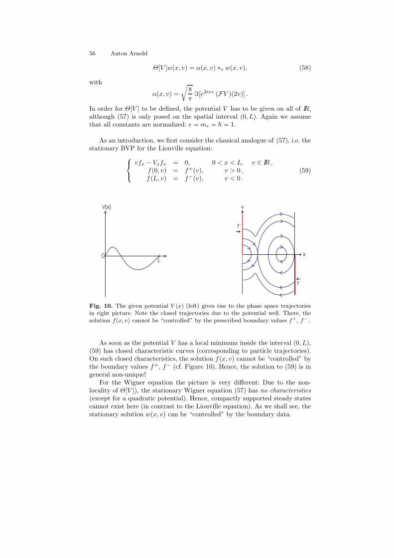
56 Anton Arnold
Θ[V ]w(x, v) = α(x, v) ∗v w(x, v), (58)
with
α(x, v) =
√
8
πℑ[e2ixv (FV )(2v)] .
In order for Θ[V ] to be defined, the potential V has to be given on all of IR,although (57) is only posed on the spatial interval (0, L). Again we assumethat all constants are normalized: e = m∗ = h = 1.
As an introduction, we first consider the classical analogue of (57), i.e. thestationary BVP for the Liouville equation:
vfx − Vxfx = 0, 0 < x < L, v ∈ IR ,f(0, v) = f+(v), v > 0 ,f(L, v) = f−(v), v < 0 .
(59)
V(x)
0L
x
v
f
f
+
-
Fig. 10. The given potential V (x) (left) gives rise to the phase space trajectoriesin right picture. Note the closed trajectories due to the potential well. There, thesolution f(x, v) cannot be “controlled” by the prescribed boundary values f+, f−.
As soon as the potential V has a local minimum inside the interval (0, L),(59) has closed characteristic curves (corresponding to particle trajectories).On such closed characteristics, the solution f(x, v) cannot be “controlled” bythe boundary values f+, f− (cf. Figure 10). Hence, the solution to (59) is ingeneral non-unique!
For the Wigner equation the picture is very different: Due to the non-locality of Θ[V ]), the stationary Wigner equation (57) has no characteristics(except for a quadratic potential). Hence, compactly supported steady statescannot exist here (in contrast to the Liouville equation). As we shall see, thestationary solution w(x, v) can be “controlled” by the boundary data.
Mathematical Properties of Quantum Evolution Equations 57
“standard” transport problems:
First we compare (57) to the structure of conventional stationary transportproblems, appearing in neutron transport, e.g. [GvMP87]. Those problems aretypically of the form
vfx −Af = 0, 0 < x < L,
with a positive Fredholm operator A. The positivity of A reflects the fact,that it models the particle interaction with a diffusive medium.
In the Wigner equation A(x) := Θ[V ] is a skew-symmetric operator onL2(IRv). Hence, it does not fall into the above class of standard transportproblems.
discrete velocity Wigner model:
Since the continuous velocity problem (57) for vwx − Θ[V ]w = 0 is notfully understood yet, we shall discuss here its semi-discretization in velocity.We make the approximation wj(x) ≈ w(x, vj) with the discrete velocitiesv1 ≥ ... ≥ vK > 0 > vK+1 ≥ ... ≥ vN . Hence, we consider the following BVPfor the vector w(x) ∈ IRN , x ∈ [0, L]:
Twx −A(x)w = 0, 0 < x < L ,
w+(0) = (w1, ..., wK)T (x = 0) = f+ ,
w−(0) = (wK+1, ..., wN )T (x = L) = f− .
(60)
Here, T is the diagonal matrix T = diag(v1, ..., vN ). In analogy to Θ[V ], thespace-dependent matrix A(x) ∈ IRN×N is skew-symmetric ∀x. Moreover,A(x)is typically a Toeplitz matrix (in analogy to (58)), but we shall not use thisfact below.
Example 7.1. We briefly illustrate, why we exclude here 0 as a discrete velocity.Consider the simple case N = 3 with v1 = 1, v2 = 0, v3 = −1. This yields thealgebro-differential equation (ADE)
ddxw1 −αw2 −βw3 = 0 ,
αw1 −γw3 = 0 ,− d
dxw3 +βw1 +γw2 = 0 ,(61)
with the (natural) BCs
w1(0) = f+, w3(L) = f− . (62)
Since w2 does not appear in the algebraic constraint (second line of (61)),the index of this ADE is 2. Hence, the BCs (62) make the above systemoverdetermined and there is either no or infinitely many solutions. This prob-lem of including 0 as a discrete velocity was already observed in numericaldiscretizations of the stationary Wigner equation [Fre90].
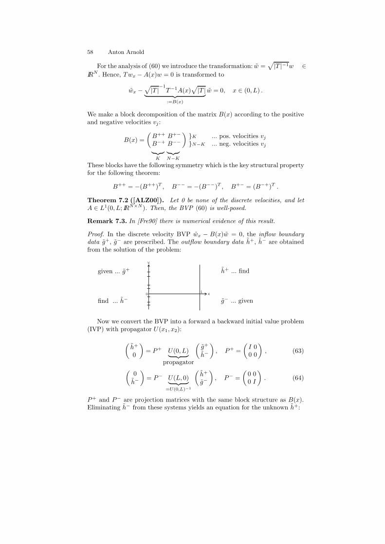
58 Anton Arnold
For the analysis of (60) we introduce the transformation: w =√
|T |−1w ∈IRN . Hence, Twx −A(x)w = 0 is transformed to
wx −√
|T |−1T−1A(x)
√
|T |︸ ︷︷ ︸
:=B(x)
w = 0, x ∈ (0, L) .
We make a block decomposition of the matrix B(x) according to the positiveand negative velocities vj :
B(x) =
(B++ B+−
B−+ B−−
)K ... pos. velocities vjN−K ... neg. velocities vj
︸︷︷︸
K
︸︷︷︸
N−K
These blocks have the following symmetry which is the key structural propertyfor the following theorem:
B++ = −(B++)T , B−− = −(B−−)T , B+− = (B−+)T .
Theorem 7.2 ([ALZ00]). Let 0 be none of the discrete velocities, and letA ∈ L1(0, L; IRN×N). Then, the BVP (60) is well-posed.
Remark 7.3. In [Fre90] there is numerical evidence of this result.
Proof. In the discrete velocity BVP wx − B(x)w = 0, the inflow boundarydata g+, g− are prescribed. The outflow boundary data h+, h− are obtainedfrom the solution of the problem:
given ... g+
find ... h−L
xo
v j
h+ ... find
g− ... given
Now we convert the BVP into a forward a backward initial value problem(IVP) with propagator U(x1, x2):
(
h+
0
)
= P+ U(0, L)︸ ︷︷ ︸
propagator
(g+
h−
)
, P+ =
(I 00 0
)
, (63)
(0
h−
)
= P− U(L, 0)︸ ︷︷ ︸
=U(0,L)−1
(
h+
g−
)
, P− =
(0 00 I
)
. (64)
P+ and P− are projection matrices with the same block structure as B(x).Eliminating h− from these systems yields an equation for the unknown h+:
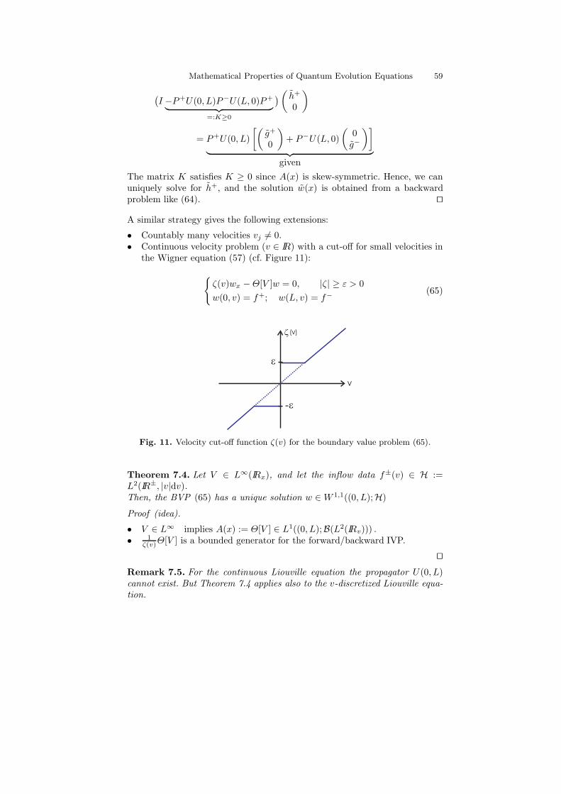
Mathematical Properties of Quantum Evolution Equations 59
(I −P+U(0, L)P−U(L, 0)P+
︸ ︷︷ ︸
=:K≥0
)(
h+
0
)
= P+U(0, L)
[(g+
0
)
+ P−U(L, 0)
(0g−
)]
︸ ︷︷ ︸
given
The matrix K satisfies K ≥ 0 since A(x) is skew-symmetric. Hence, we canuniquely solve for h+, and the solution w(x) is obtained from a backwardproblem like (64). ⊓⊔
A similar strategy gives the following extensions:
• Countably many velocities vj 6= 0.• Continuous velocity problem (v ∈ IR) with a cut-off for small velocities in
the Wigner equation (57) (cf. Figure 11):
ζ(v)wx −Θ[V ]w = 0, |ζ| ≥ ε > 0
w(0, v) = f+; w(L, v) = f−(65)
v
e
e-
z (v)
Fig. 11. Velocity cut-off function ζ(v) for the boundary value problem (65).
Theorem 7.4. Let V ∈ L∞(IRx), and let the inflow data f±(v) ∈ H :=L2(IR±, |v|dv).Then, the BVP (65) has a unique solution w ∈W 1,1((0, L);H)
Proof (idea).
• V ∈ L∞ implies A(x) := Θ[V ] ∈ L1((0, L);B(L2(IRv))) .• 1
ζ(v)Θ[V ] is a bounded generator for the forward/backward IVP.
⊓⊔Remark 7.5. For the continuous Liouville equation the propagator U(0, L)cannot exist. But Theorem 7.4 applies also to the v-discretized Liouville equa-tion.
60 Anton Arnold
7.2 Exponential Convergence to Steady State
We consider now the time dependent analogue of (60), i.e. the IBVP forthe Wigner equation with discrete velocities. We make the approximationwj(x, t) ≈ w(x, vj , t), j ∈ J ⊂ ZZ. The discrete velocity Wigner function
w(x, t) ∈ IRN satisfies the following linear hyperbolic system:
wt + Twx −A(x)w = 0, 0 < x < L, t > 0
w+(0, t) = f+; w−(L, t) = f−,
w(x, 0) = wI .
(66)
As before, we assume T = diag(vj)j∈J and 0 6∈ vjj∈J . The matrix A(x) isskew-symmetric for all x and (usually) some v-discretization of the operatorΘ[V ].
Theorem 7.6 ([ACT02]). Let wI ∈ L2(0, L)×ℓ2(J), f± ∈ H := ℓ2(J ; |vj |),and A ∈ L∞((0, L);B(ℓ2(J))).Then,
w(., t)t→∞−→ w∞ in L2(0, L) × ℓ2(J) with some exponential rate ε > 0.
w∞ is the unique steady state of (66), provided by the results of §7.1.
Remark 7.7. Since A(x) is skew-symmetric, the system (66) does not showany damping. The exponential decay towards the steady state is only due tooutflow through the boundary.
Proof. Transforming to homogeneous inflow BCs via w := w − w∞ yields:
wt + T wx −A(x)w = 0
w+(0, t) = 0; w−(L, t) = 0
w(x, z) = wI − w∞
(67)
• A naive approach in L2(0, L) would only yield ddt‖w‖L2(0,L) ≤ 0, but no
decay estimate.• Hence, we shall prove the decay in a weighted L2-norm. To this end we
construct a multiplier matrix Φ(x) = diag(ϕj(x))j∈J with:
0 < c ≤ ϕj(x) ≤ C ∀j ∈ J, x ∈ [0, L]
• We take the L2(0, L)–inner product of (67) with Φw. With the notation
‖w‖2Φ :=
∫ L
0
w⊤ · Φ · w dx
we have1
2
d
dt‖w‖2
Φ − 1
2〈w, TΦxw〉L2 − 〈Aw, Φw〉L2 ≤ 0 .
The last inequality is due to outflow at the boundary.
Mathematical Properties of Quantum Evolution Equations 61
• Now we have to find a matrix function Φ(x) such that the following in-equality holds for some (small) ε > 0:
12
(f, TΦx(x)f
)+
(A(x)f, Φ(x)f
)≤ −ε
(f, Φ(x)f
)
∀x ∈ [0, L], ∀f ∈ IR|J|
• This holds true, if we have componentwise (i.e. ∀j ∈ J):
1
2vj∂
∂xϕj +
1
2
∑
i6=j
|aij(x)||ϕi − ϕj | ≤ −εϕj on [0, L] .
• After constructing these functions ϕj , we obtain:
d
dt‖w‖Φ ≤ −ε ‖w‖Φ := −ε
∥∥√ϕjwj(., t)
∥∥L2(0,L)
.
⊓⊔
open problems:
• Removing the velocity cut-off (ζ(v) −→ v) makes 1ζ(v)Θ[V ] an unbounded
operator in the forward/backward IVPs involved in (63), (64). In this caseit is not yet clear how to construct the propagator U(0, L).
• To find conditions on f± such that ˆ[w] ≥ 0 or at least n(x) =∫
IR w(x, v) dv≥ 0 on [0, L] seems to be very difficult. Actually, the Wigner framework isprobably not appropriate to answer this question.
• Non-linear (self-consistent) extension of (57):
vwx −Θ[V ]w = 0, 0 < x < L, v ∈ IR ,Vxx = D(x) −
∫
IRw(x, v) dv, 0 < x < L,
w(0, v) = f+(v), v > 0 ,w(L, v) = f−(v), v < 0 .
would need estimates on the quantum-repulsive/attractive potential. Here,some strategies from the stationary quantum-classical coupling in [Ben98]might be extendable.
References
[AABES07] Antoine, X., Arnold, A., Besse, C., Ehrhardt, M., and Schadle A.: AReview of Transparent and Artificial Boundary Conditions Techniquesfor Linear and Nonlinear Schrodinger Equations, submitted to Appl.Num. Mathem. (2007)
62 Anton Arnold
[ACD02] Arnold, A., Carrillo, J.A., Dhamo, E.: The periodic Wigner-Poisson-Fokker-Planck system. JMAA, 275, 263–276 (2002)
[ACT02] Arnold, A., Carrillo, J.A., Tidriri, M.D.: Large-time behavior of discretekinetic equations with non-symmetric interactions. Math. Models Meth.Appl. Sc., 12, no.11, 1555–1564 (2002)
[ADM07] Arnold, A., Dhamo, E., Manzini, C.: The Wigner-Poisson-Fokker-Planck system: global-in-time solutions and dispersive effects. Annalesde l’IHP (C) - Analyse non lineaire 24, no.4, 645–676 (2007)
[ADM07a] Arnold, A., Dhamo, E., Manzini, C.: Dispersive effects in quantum ki-netic equations. Indiana Univ. Math. J., 56, no.3, 1299–1331 (2007)
[AF01] Alicki, R., Fannes, M.: Quantum Dynamical Systems. Oxford Univer-sity Press (2001)
[AGGS07] Arnold, A., Gamba, I.M., Gualdani, M.P., Sparber, C.: The Wigner-Fokker-Planck equation: Stationary states and large time behavior. sub-mitted (2007)
[AJ06] Arnold, A., Jungel, A.: Multi-scale modeling of quantum semiconductordevices. , p. 331–363 in: Analysis, Modeling and Simulation of Multi-scale Problems, A. Mielke (Ed.), Springer, Berlin-Heidelberg (2006)
[AJP06] Attal, S., Joye, A., Pillet, C.A. (Eds.): Open Quantum Systems I-III -Lecture Notes in Mathematics, 1880–1882, Springer, Berlin-Heidelberg(2006)
[ALMS04] Arnold, A., Lopez, J.L., Markowich, P., Soler, J.: An analysis ofquantum Fokker-Planck models: A Wigner function approach. RevistaMatem. Iberoam., 20, no.3, 771–814 (2004)
[ALZ00] Arnold, A., Lange, H., Zweifel, P.F.: A discrete-velocity, stationaryWigner equation. J. Math. Phys., 41, no.11, 7167–7180 (2000)
[AMTU01] Arnold, A., Markowich, P., Toscani, G., Unterreiter, A.: Comm. PDE,26, no.1–2, 43–100 (2001)
[AN91] Arnold, A., Nier, F.: The two-dimensional Wigner-Poisson problem foran electron gas in the charge neutral case. Math. Meth. Appl. Sc., 14,595–613 (1991)
[Arn96] Arnold, A.: Self-consistent relaxation-time models in quantum mechan-ics. Comm. PDE, 21, no.3&4, 473–506 (1996)
[Arn96a] Arnold, A.: The relaxation-time von Neumann-Poisson equation. Pro-ceedings of ICIAM 95, Hamburg (1995), Mahrenholtz, O., Mennicken,R. (eds.); ZAMM 76 S2 (1996)
[Arn01] Arnold, A.: Mathematical concepts of open quantum boundary condi-tions. Transp. Theory Stat. Phys., 30, no.4–6, 561–584 (2001)
[Arn02] Arnold, A.: Entropy method and the large-time behaviorof parabolic equations. Lecture notes for the XXVII Sum-mer school in mathematical physics, Ravello, Italy (2002).http://www.anum.tuwien.ac.at/˜arnold/papers/ravello.pdf
[AS07] Arnold, A., Schulte, M.: Transparent boundary conditions for quantum-waveguide simulations. to appear in Mathematics and Computers inSimulation (2007), Proceedings of MATHMOD 2006, Vienna, Austria.
[AS04] Arnold, A., Sparber, C.: Conservative Quantum Dynamical Semigroupsfor mean-field quantum diffusion models. Comm. Math. Phys., 251,no.1 179–207 (2004)
[Ben98] Ben Abdallah, N.: A Hybrid Kinetic-Quantum Model for StationaryElectron Transport. J. Stat. Phys., 90, no.3–4, 627–662 (1998)
Mathematical Properties of Quantum Evolution Equations 63
[Bre87] Brezis, H.: Analyse fonctionelle - Theorie et applications. Masson (1987)[BM91] Brezzi, F., Markowich, P.A.: The three-dimensional Wigner-Poisson
problem: existence, uniqueness and approximation. Math. MethodsAppl. Sci., 14, no.1, 35–61 (1991)
[BMP05] Ben Abdallah, N., Mehats, F., Pinaud, O.: On an open transientSchrodinger-Poisson system. Math. Models Methods Appl. Sci., 15,no.5, 667–688 (2005)
[BN88] Benatti, F., Narnhofer, H.: Entropy Behaviour under Completely Pos-itive Maps. Lett. Math. Phys., 15, 325–334 (1988)
[Boh89] Bohm, D.: Quantum Theory. Dover (1989); reprint from 1951.[Cas97] Castella, F.: L2–solutions to the Schrodinger-Poisson System: Exis-
tence, Uniqueness, Time Behaviour, and Smoothing Effects. Math.Mod. Meth. Appl. Sci., 7, no.8, 1051–1083 (1997)
[Cas98] Castella, F.: The Vlasov-Poisson-Fokker-Planck System with InfiniteKinetic Energy. Indiana Univ. Math. J., 47, no.3, 939–964 (1998)
[Caz96] Cazenave, T.: An introduction to nonlinear Schrodinger equation. Tex-tos de Metodos Matematicos 26, Univ. Federal do Rio de Janeiro,(1996)
[CEFM00] Castella, F., Erdos, L., Frommlet, F., Markowich, P.A.: Fokker-Planckequations as Scaling limits of Reversible Quantum Systems. J. Statist.Phys., 100, no.3-4, 543–601 (2000)
[CL83] Caldeira, A.O., Leggett, A.J.: Path integral approach to quantum Brow-nian motion. Physica A, 121, 587–616 (1983)
[CLN04] Canizo, J.A., Lopez, J.L., Nieto, J.: Global L1–theory and regularityfor the 3D nonlinear Wigner-Poisson-Fokker-Planck system. J. Diff. Eq.,198, 356–373 (2004)
[CP96] Castella, F., Perthame, B.: Estimations de Strichartz pour les Equationsde transport Cinetique. C. R. Acad. Sci. Paris, t. 322, Serie I, 535–540(1996)
[Dav76] Davies, E.B.: Quantum Theory of Open Systems. Academic Press,London-New York (1976)
[Dav77] Davies, E.B.: Quantum dynamical semigroups and the neutron diffusionequation. Rep. Math. Phys., 11, no.2, 169–188 (1977)
[Deg] Degond, P.: Introduction a la theorie quantique, DEA–Lecture Notes,UPS Toulouse.
[DL88] Dautray, R., Lions, J.L.: Mathematical Analysis and Numerical Meth-ods of Science and Technology; vol 1 Pysical Origins and Classical Meth-ods. Springer (1990)
[DL88a] Dautray, R., Lions, J.L.: Mathematical Analysis and Numerical Meth-ods of Science and Technology; vol 5 Evolution Problems I. Springer(1988)
[FR98] Fagnola, F., Rebolledo, R.: The approach to equilibrium of a classof quantum dynamical semigroups. Infinite Dim. Analysis, QuantumProb. and Rel. Topics, 1, no.4, 561–572 (1998)
[Fre90] Frensley, W.R.: Boundary conditions for open quantum systems drivenfar from equilibrium. Rev. Mod. Phys., 62, 745–791 (1990)http://www.utdallas.edu/˜frensley/technical/opensyst/opensyst.html
[Fre94] Frensley, W.R.: Quantum Transport. In: Frensley, W.R., Einspruch,N.G. (eds.) Heterostructures and Quantum Devices. Academic Press,
64 Anton Arnold
San Diego (1994)http://www.utdallas.edu/˜frensley/technical/qtrans/qtrans.html
[GvMP87] Greenberg, W., van der Mee, C., Protopopescu, V.: Boundary ValueProblems in Abstract Kinetic Theory. Birkhauser, Basel-Boston-Stuttgart (1997)
[GV94] Ginibre, J., Velo, G.: The global Cauchy problem for the non linearSchrodinger equation revisited. Annales de l’institut Henri Poincare(C) Analyse non lineaire, 2, no.4, 309–327 (1985)
[HO89] Hayashi, N., Ozawa, T.: Smoothing Effect for Some Schrodinger Equa-tions. J. Funct. Anal, 85, 307–348 (1989)
[ILZ94] Illner, R., Lange, H., Zweifel, P.: Global existence, uniqueness,and asymptotic behaviour of solutions of the Wigner-Poisson andSchrodinger systems. Math. Meth. Appl. Sci., 17, 349–376 (1994)
[KKFR89] Kluksdahl, N.C., Kriman, A.M., Ferry, D.K., Ringhofer, C.: Self-consistent study of the resonant-tunneling diode. Phys. Rev. B, 39,7720–7735 (1989)
[KN06] Kosina, H., Nedjalkov, M.: Wigner Function-Based Device Modeling,§67. In: Handbook of Theoretical and Computational Nanotechnology.Rieth, M., Schommers, W. (eds.) American Scientific Publishers. (2006)
[Lev70] Levinson, I.B.: Translational invariance in uniform fields and the equa-tion for the density matrix in the Wigner representation. Sov. Phys.JETP, 30, 362–367 (1970)
[Lin76] Lindblad, G.: On the generators of quantum mechanical semigroups.Comm. Math. Phys., 48, 119–130 (1976)
[LK90] Lent, C.S., Kirkner, D.J.: The quantum transmitting boundary method,J. of Appl. Phys., 67, nr.10, 6353–6359 (1990)
[LL85] Landau, L.D., Lifschitz, E.M.: Quantenmechanik. Akademie-Verlag,Berlin. (1985)
[LP93] Lions, P.L., Paul, T.: Sur les measures de Wigner, Rev. Math. Iberoam.,9, no.3, 553–618 (1993)
[LT76] Lieb, E.H., Thirring, W.E.: Inequalities for the moments of the eigen-values of the Schrodinger Hamiltonian and their relation to Sobolevinequalities. In: Lieb, E.H., Simon, B., Wightman, A.S. (eds.) Stud-ies in Mathematical Physics. Essays in honor of Valentine Bargmann.Princeton Univ. Press (1976)
[MRS90] Markowich, P.A., Ringhofer, C.A., Schmeiser, C.: Semiconductor Equa-tion. Springer-Verlag, Wien-New York. (1990)
[Paz83] Pazy:, A. Semigroups of Linear Operators and Applications to PartialDifferential Equations. Springer, New York (1983)
[Per96] Perthame, B.: Time decay, propagation of low moments and dispersiveeffects for kinetic equations. Comm. P.D.E., 21, no.1&2, 659–686 (1996)
[Rin03] Ringhofer, C.: Thermodynamic principles in modeling nano-scale trans-port in semiconductors. Lecture Notes for: Nanolab Spring School.Toulouse (2003)http://math.la.asu.edu/˜chris/nano030529.pdf
[RS75] Reed, M., Simon, B.: Methods of modern mathematical physics. II.Fourier analysis, self-adjointness. Academic Press (1975)
[SA07] Schulte, M., Arnold, A.: Discrete transparent boundary conditions forthe Schrodinger equation – a compact higher order scheme. Preprint(2007)
Mathematical Properties of Quantum Evolution Equations 65
[SS87] Sandulescu, A., Scutaru, H.: Open Quantum Systems and the Dampingof Collective Modes in Deep Inelastic Collisions. Annals of Phys., 173,277–317 (1987)
[SCDM04] Sparber, C., Carrillo, J.A., Dolbeault, J., Markowich, P.A.: Onthe Long-Time Behavior of the Quantum Fokker-Planck Equation.Monatsh. Math., 141, 237–257 (2004)
[Sim79] Simon, B.: Trace Ideals and Their Applications. Cambridge UniversityPress (1979)
[Spo76] Spohn, H.: Approach to equilibrium for completely positive dynamicalsemigroups. Rep. Math. Phys., 10, no.2, 189–194 (1976)
[Spo77] Spohn, H.: Entropy production for quantum dynamical semigroups. J.Math. Phys., 19, no.5, 1227–1230 (1978)
[Tha05] Thaller, B.: Advanced Visual Quantum Mechanics. Springer (2005)[W32] Wigner, E.: On the quantum correction for thermodynamic equilibrium.
Phys. Rev., 40, 749–759 (1932)