Embed Size (px)
Citation preview

Application of quantum Hamilton equationsMichael Beyer1, Jeanette Köppe1, Markus Patzold1, Wilfried Grecksch2,Wolfgang Paul1
1Institute for physicsMartin-Luther-Universität Halle-Wittenberg2Institute for mathematicsMartin-Luther-Universität Halle-Wittenberg
30th Nov 2017Michael Beyer (MLU) QHE 30th Nov 2017 1 / 15

OutlineNelson’s stochastic mechanicsStochastic Mechanics as an optimal control problem(Derivation of quantum Hamilton equations)Numerical algorithmResults for stationary problems
> Double-well potential> Excited states> Simple multidimensional systemsMichael Beyer (MLU) QHE 30th Nov 2017 2 / 15

IntroductionAnalogy between classical and quantum mechanicsClassical mechanicsHamilton principle
S [x ] = ∫ T0{ 1
2 mv (t)− V (x , t)}dt
Hamilton-Jacobi equation
∂t S(x , t)− V (x , t)− 12m (∇x S(x , t))2 = 0
Newton’s equations
x (t) = v (t) , m a(t) = F = −∇x V (x , t)
Michael Beyer (MLU) QHE 30th Nov 2017 3 / 15

IntroductionAnalogy between classical and quantum mechanicsClassical mechanicsHamilton principle
S [x ] = ∫ T0{ 1
2 mv (t)− V (x , t)}dt
Hamilton-Jacobi equation
∂t S(x , t)− V (x , t)− 12m (∇x S(x , t))2 = 0
Newton’s equations
x (t) = v (t) , m a(t) = F = −∇x V (x , t)Quantum mechanics
Schrödinger equation
i~ ∂tΨ(x , t) = [− ~22m ∆ + V (x , t)]Ψ(x , t)
Kinematic equations
dx (t) = [v (x , t) + u(x , t)]dt +√ ~m dWf (t) , E[ma(t)] = Fdx (t) = [v (x , t)− u(x , t)]dt +√ ~m dWb (t)
E. Nelson, Phys. Rev., 150: 1079-1085, 1966
v (x , t) = ∇x Im[ln Ψ]m , u(x , t) = ~
m∇x Re [ln Ψ]
Quantum Hamilton principleJ [x ] = E
[∫ T0{ 1
2 m(v − iu)2 − V (x , t)}dt + Φ0(x0)]M. Pavon, J. Math. Phys., 36: 6774-6800, 1995
Michael Beyer (MLU) QHE 30th Nov 2017 3 / 15

Brief Introduction to the formalism Nelson’s stochastic mechanicsNelson’s stochastic mechanicsE. Nelson, Derivation of the Schrödinger equation from Newtonian mechanics. Phys. Rev. 150, 1079 (1966)
forward backward stochastic differential equations (FBSDE)dx (t) = [v (t, x (t)) + u(t, x (t))]dt + σdW (t) , x (t0) = x0dx (t) = [v (t, x (t))− u(t, x (t))]dt + σdW∗(t) , x (T ) = xT
Nelson: particles subjected to conservative Brownian motion (diffusionprocess) where interaction with the environment can not be neglecteddiffusion coefficient σ2 = ~m E[ma] = −∂xV (x , t)
equivalent to Schrödinger equation, if wavefunction has the formψ(x , t) = exp{R(x , t) + i S(x , t)}
Michael Beyer (MLU) QHE 30th Nov 2017 4 / 15

Brief Introduction to the formalism Nelson’s stochastic mechanicsExample: double slit (electrons)with known v and u → create realizations of quantum point particles
N = 1
Michael Beyer (MLU) QHE 30th Nov 2017 5 / 15

Brief Introduction to the formalism Nelson’s stochastic mechanicsExample: double slit (electrons)with known v and u → create realizations of quantum point particles
N = 20
Michael Beyer (MLU) QHE 30th Nov 2017 5 / 15

Brief Introduction to the formalism Nelson’s stochastic mechanicsExample: double slit (electrons)with known v and u → create realizations of quantum point particles
N = 400
Michael Beyer (MLU) QHE 30th Nov 2017 5 / 15

Brief Introduction to the formalism Nelson’s stochastic mechanicsExample: double slit (electrons)with known v and u → create realizations of quantum point particles
N = 800
problem: solution of Schrödinger equation is needed to get the velocities v , uMichael Beyer (MLU) QHE 30th Nov 2017 5 / 15

Brief Introduction to the formalism Nelson’s stochastic mechanicsExample: double slit (electrons)with known v and u → create realizations of quantum point particles
N = 800
problem: solution of Schrödinger equation is needed to get the velocities v , uMichael Beyer (MLU) QHE 30th Nov 2017 5 / 15

Brief Introduction to the formalism Quantum Hamilton principle as control problemStochastic optimal control problemHamilton’s principle: extremize action functional w. r. t. x
J [x ] = ∫ T
0L(t, x (t), x (t)) dt Lagrangian L = T − V
Quantum Hamilton principle as stoch. optimal control problem [3, 1]:maximization of cost function J with L as (stochastic) Lagrange functionJ [vq ] = E
[∫ T
0L(t, x (t), vq(t, x (t)))dt + Φ(x0)]
subject to the constraint (controlled equation)dx (t) = vq(t, x (t))dt + 1
2σ((1 + i)dW (t) + (1− i)W∗(t)) , x (0) = x0
vq is the quantum velocity vq = v − iu and the optimal feedback control to x (t)vq = vq(t, x (t))
Michael Beyer (MLU) QHE 30th Nov 2017 6 / 15

Brief Introduction to the formalism Quantum Hamilton principle as control problemQuantum Hamilton equationsJ. Koeppe et. al, Derivation and application of quantum Hamilton equations of motion. Annalen der Physik 529, 1600251 (2017)
coupled forward backward SDEs [1]dx (t) = [v (t, x ) + u(t, x )]dt + σdW (t)dx (t) = [v (t, x )− u(t, x )]dt + σdW∗(t)
m d[v (t, x ) + u(t, x )] = ∂xV (x , t)dt + q(t) dW∗(t)taking the classical limit (u, ~/m→ 0)dx (t) = v (x , t)dt , mdv = −∂x V (x , t)dttaking the expectation value one recovers Ehrenfest’s theoremdE[x (t)] = E[v (x , t)]dt , mdE[v (t)] = −E[∂x V (x , t)]dt
Michael Beyer (MLU) QHE 30th Nov 2017 7 / 15

Numerical approachTowards a numerical solution→ problem: four unknown stochastic processes x , v , u, qconsider stationary case v ≡ 0, all information is stored in u, e. g.
ρ(x ) = exp [ 2σ2
∫C
u(x ′) · dx ′]
discretize time axis, e. g. using Euler-Mayurama Schemexπ (ti+1) = xπ (ti ) + uπ (xπ (ti ))∆t + σ∆W (ti )
uπ (xπ (ti )) = u(xπ (ti+1))− ∂x V (xπ (ti ))∆t − qπ (ti )∆W∗(ti )due to Markov property the backward equation can be calculated withthe help of conditional expectation
uπ (xπ (ti )) = E[uπ (xπ (ti+1))|xπ (ti )]− ∂x V (xπ (ti ))∆t
this is usually the crucial point of a numerical approach when solvingcoupled FBSDE or BSDE, because the numerical calculation is not trivialMichael Beyer (MLU) QHE 30th Nov 2017 8 / 15
Numerical approachIteration schemeiteration scheme for u0 choose starting value u (x ) ≡ 01 use u to generate N paths with nt steps2 integrate u backward in time3 average u(x (ti )) over intervals → u (x ) = 〈u(x (ti ))〉cube4 go to 1
1D harmonic oscillatorV (x ) = 1
2 mω2x2
xπ (ti+1) = xπ (ti ) + uπ (xπ (ti ))∆t + σ∆W (ti )uπ (xπ (ti )) = E[uπ (xπ (ti+1))|xπ (ti )]− ∂x V (xπ (ti ))∆t
x (a.u.)4− 2− 0 2 4
osm
otic
vel
ocity
(a.
u.)
4−
2−
0
2
4opt. control
exact
Michael Beyer (MLU) QHE 30th Nov 2017 9 / 15

Numerical approachIteration schemeiteration scheme for u0 choose starting value u (x ) ≡ 01 use u to generate N paths with nt steps2 integrate u backward in time3 average u(x (ti )) over intervals → u (x ) = 〈u(x (ti ))〉cube4 go to 1
1D harmonic oscillatorV (x ) = 1
2 mω2x2
xπ (ti+1) = xπ (ti ) + uπ (xπ (ti ))∆t + σ∆W (ti )uπ (xπ (ti )) = E[uπ (xπ (ti+1))|xπ (ti )]− ∂x V (xπ (ti ))∆t
x (a.u.)4− 2− 0 2 4
osm
otic
vel
ocity
(a.
u.)
4−
2−
0
2
4opt. control
exact
Michael Beyer (MLU) QHE 30th Nov 2017 9 / 15

Numerical approachIteration schemeiteration scheme for u0 choose starting value u (x ) ≡ 01 use u to generate N paths with nt steps2 integrate u backward in time3 average u(x (ti )) over intervals → u (x ) = 〈u(x (ti ))〉cube4 go to 1
1D harmonic oscillatorV (x ) = 1
2 mω2x2
xπ (ti+1) = xπ (ti ) + uπ (xπ (ti ))∆t + σ∆W (ti )uπ (xπ (ti )) = E[uπ (xπ (ti+1))|xπ (ti )]− ∂x V (xπ (ti ))∆t
x (a.u.)4− 2− 0 2 4
osm
otic
vel
ocity
(a.
u.)
4−
2−
0
2
4opt. control
exact
Michael Beyer (MLU) QHE 30th Nov 2017 9 / 15

Numerical approachIteration schemeiteration scheme for u0 choose starting value u (x ) ≡ 01 use u to generate N paths with nt steps2 integrate u backward in time3 average u(x (ti )) over intervals → u (x ) = 〈u(x (ti ))〉cube4 go to 1
1D harmonic oscillatorV (x ) = 1
2 mω2x2
xπ (ti+1) = xπ (ti ) + uπ (xπ (ti ))∆t + σ∆W (ti )uπ (xπ (ti )) = E[uπ (xπ (ti+1))|xπ (ti )]− ∂x V (xπ (ti ))∆t
x (a.u.)4− 2− 0 2 4
osm
otic
vel
ocity
(a.
u.)
4−
2−
0
2
4opt. control
exact
Michael Beyer (MLU) QHE 30th Nov 2017 9 / 15
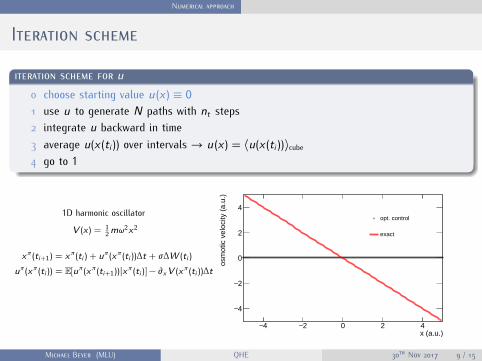
Numerical approachIteration schemeiteration scheme for u0 choose starting value u (x ) ≡ 01 use u to generate N paths with nt steps2 integrate u backward in time3 average u(x (ti )) over intervals → u (x ) = 〈u(x (ti ))〉cube4 go to 1
1D harmonic oscillatorV (x ) = 1
2 mω2x2
xπ (ti+1) = xπ (ti ) + uπ (xπ (ti ))∆t + σ∆W (ti )uπ (xπ (ti )) = E[uπ (xπ (ti+1))|xπ (ti )]− ∂x V (xπ (ti ))∆t
u(x ) after 50 iterations
x (a.u.)4− 2− 0 2 4
osm
otic
vel
ocity
(a.
u.)
4−
2−
0
2
4opt. control
exact
Michael Beyer (MLU) QHE 30th Nov 2017 9 / 15

Numerical resultsDouble well: ground state V (x ) = V0a4 (x2 − a2)2 V0 = 2, a = 1.5
0
0.1
0.2
0.3
0.4
-4 -3 -2 -1 0 1 2 3 4
Pro
babi
lity
dens
ity p
(x)
Position x
NumerovOpt. Cont.
0
1
2
3
4
-2 0 2
V(x)
Michael Beyer (MLU) QHE 30th Nov 2017 10 / 15

Numerical results Excited states with SUSYSUSY in stochastic mechanicsH0 = Q+
0 ·Q−0 + E0 → H1 = Q−0 ◦Q+0
e. g. for the Hamiltonian Hi in cartesian coordinatesQ±i = ∓∇− u i
Michael Beyer (MLU) QHE 30th Nov 2017 11 / 15

Numerical results Excited states with SUSYDouble well: excited states V (x ) = V0a4 (x2 − a2)2 V0 = 1, a = 1.5
Tunnel splitting is given by the mean first passage timePerturbation theory prediction for the splitting is not correct}→ Poster
Michael Beyer (MLU) QHE 30th Nov 2017 12 / 15

Numerical results Excited states with SUSYDouble well: excited states V (x ) = V0a4 (x2 − a2)2 V0 = 1, a = 1.5
Tunnel splitting is given by the mean first passage timePerturbation theory prediction for the splitting is not correct}→ Poster
Michael Beyer (MLU) QHE 30th Nov 2017 12 / 15

Numerical results Multidimensional systemsHigher dimensional systems2D isotropic harmonic oscillator
-3-2
-1 0
1 2
3-3
-2
-1
0
1
2
3
-0.6-0.4-0.2
0 0.2 0.4 0.6
Ψ01
(x,y
)
x
y
Ψ01
(x,y
) -0.6-0.4-0.2 0 0.2 0.4 0.6
3D hydrogen atom
Spherical problemsdr = (ur + σ 2
r
)dt + σdW
µdur = 1r 2
(~ur + ∂r V (r ))dt + (qdW ∗)rhydrogen atom
0
0.2
0.4
0.6
0 1 2 3 4 5
Wav
e fu
nctio
n Ψ
100(
r) (
Ryd
berg
uni
ts)
Distance r (Bohr radius a0)
exactOpt. Cont.
-2
-1
0
0 2 4
radial part of the osmotic velocity ur(r)=-2
r
Michael Beyer (MLU) QHE 30th Nov 2017 13 / 15

SummaryDerivation of kinematic and dynamic equations for non-relativisticquantum system → quantum Hamilton equationsNumerical algorithm to solve these stochastic equations in the stationarycase without using the Schrödinger equationSolution to (simple) problems in higher dimensionsDetermination of all excited eigenstates of the Schrödinger equation
Future work> Solving non-stationary problems numerically> Extending to relativistic particles and spin
Michael Beyer (MLU) QHE 30th Nov 2017 14 / 15

LiteratureLiterature IJ. Köppe, W. Grecksch, and W. Paul.Derivation and application of quantum hamilton equations of motion.Annalen der Physik, 529(3):1600251–n/a, 2017.1600251.Edward Nelson.Derivation of the schrödinger equation from newtonian mechanics.Physical Review, 150(4):1079, 1966.Michele Pavon.Hamilton’s principle in stochastic mechanics.Journal of Mathematical Physics, 36(12):6774–6800, 1995.
Michael Beyer (MLU) QHE 30th Nov 2017 15 / 15

Thank you for your attention!
Michael Beyer (MLU) QHE 30th Nov 2017 15 / 15

Nelson’s stochastic mechanicsE. Nelson, Derivation of the Schrödinger equation from Newtonian mechanics. Phys. Rev. 150, 1079 (1966)
forward backward stochastic differential equations (FBSDE)dx (t) = [v (t, x (t)) + u(t, x (t))]dt + σdW (t) , x (t0) = x0dx (t) = [v (t, x (t))− u(t, x (t))]dt + σdW∗(t) , x (T ) = xTwhere:- x (t) = x (t, ω) is a stochastic process in Rn·d- x (t) is connected to a probability distribution ρ satisfying a forward andbackward Fokker-Planck equation- W (t) is a n · d dimensional Wiener processes- current velocity v = σ2∇S(t, x (t))- E[v ] = 〈p〉Ψ- osmotic velocity u = σ2∇R(t, x (t)) = σ2∇ln ρ(t, x (t))- E[u] = 0 and E[v2 + u2] = ⟨ (∆p/m)2 ⟩Ψ
Michael Beyer (MLU) QHE 30th Nov 2017 15 / 15


![1.7cm Lecture 3: [1ex] Hamilton-Jacobi-Bellman Equations ... · Lecture 3: Hamilton-Jacobi-Bellman Equations Distributional Macroeconomics Part IIof ECON2149 Benjamin Moll Harvard](https://img.dokumen.tips/doc/110x75/5f12565ca5408c7a5b08569d/17cm-lecture-3-1ex-hamilton-jacobi-bellman-equations-lecture-3-hamilton-jacobi-bellman.jpg)