Periodic solutions for evolution equations

Electronic Journal of Differential Equations, Monogrpah 03, 2002.ISSN: 1072-6691. URL: http://ejde.math.swt.edu or http://ejde.math.unt.eduftp ejde.math.swt.edu (login: ftp)

Periodic solutions for evolution equations ∗

Mihai Bostan

Abstract

We study the existence and uniqueness of periodic solutions for evolu-tion equations. First we analyze the one-dimensional case. Then for arbi-trary dimensions (finite or not), we consider linear symmetric operators.We also prove the same results for non-linear sub-differential operatorsA = ∂ϕ where ϕ is convex.

Contents

1 Introduction 1

2 Periodic solutions for one dimensional evolution equations 22.1 Uniqueness . . . . . . . . . . . . . . . . . . . . . . . . . . . . . . 22.2 Existence . . . . . . . . . . . . . . . . . . . . . . . . . . . . . . . 52.3 Sub(super)-periodic solutions . . . . . . . . . . . . . . . . . . . . 10

3 Periodic solutions for evolution equations on Hilbert spaces 163.1 Uniqueness . . . . . . . . . . . . . . . . . . . . . . . . . . . . . . 173.2 Existence . . . . . . . . . . . . . . . . . . . . . . . . . . . . . . . 173.3 Periodic solutions for the heat equation . . . . . . . . . . . . . . 313.4 Non-linear case . . . . . . . . . . . . . . . . . . . . . . . . . . . . 34

1 Introduction

Many theoretical and numerical studies in applied mathematics focus on perma-nent regimes for ordinary or partial differential equations. The main purpose ofthis paper is to establish existence and uniqueness results for periodic solutionsin the general framework of evolution equations,

x′(t) +Ax(t) = f(t), t ∈ R, (1)

∗Mathematics Subject Classifications: 34B05, 34G10, 34G20.Key words: maximal monotone operators, evolution equations, Hille-Yosida’s theory.c©2002 Southwest Texas State University.

Submitted May 14, 2002. Published August 23, 2002.

1

2 Periodic solutions for evolution equations

by using the penalization method. Note that in the linear case a necessarycondition for the existence is

〈f〉 :=1T

∫ T

0

f(t)dt ∈ Range(A). (2)

Unfortunately, this condition is not always sufficient for existence; see the exam-ple of the orthogonal rotation of R2. Nevertheless, the condition (2) is sufficientin the symmetric case. The key point consists of considering first the perturbedequation

αxα(t) + x′α(t) +Axα(t) = f(t), t ∈ R,where α > 0. By using the Banach’s fixed point theorem we deduce the existenceand uniqueness of the periodic solutions xα, α > 0. Under the assumption (2),in the linear symmetric case we show that (xα)α>0 is a Cauchy sequence in C1.Then by passing to the limit for α → 0 it follows that the limit function is aperiodic solution for (1).

These results have been announced in [2]. The same approach applies forthe study of almost periodic solutions (see [3]). Results concerning this topichave been obtained previously by other authors using different methods. Asimilar condition (2) has been investigated in [5] when studying the range ofsums of monotone operators. A different method consists of applying fixedpoint techniques, see for example [4, 7].

This article is organized as follows. First we analyze the one dimensionalcase. Necessary and sufficient conditions for the existence and uniqueness of pe-riodic solutions are shown. Results for sub(super)-periodic solutions are provedas well in this case. In the next section we show that the same existence resultholds for linear symmetric maximal monotone operators on Hilbert spaces. Inthe last section the case of non-linear sub-differential operators is considered.

2 Periodic solutions for one dimensional evolu-tion equations

To study the periodic solutions for evolution equations it is convenient to con-sider first the one dimensional case

x′(t) + g(x(t)) = f(t), t ∈ R, (3)

where g : R → R is increasing Lipschitz continuous in x and f : R → R isT -periodic and continuous in t. By Picard’s theorem it follows that for eachinitial data x(0) = x0 ∈ R there is an unique solution x ∈ C1(R;R) for (3). Weare looking for T -periodic solutions. Let us start by the uniqueness study.

2.1 Uniqueness

Proposition 2.1 Assume that g is strictly increasing and f is periodic. Thenthere is at most one periodic solution for (3).

Mihai Bostan 3

Proof Let x1, x2 be two periodic solutions for (3). By taking the differencebetween the two equations and multiplying by x1(t)− x2(t) we get

12d

dt|x1(t)− x2(t)|2 + [g(x1(t))− g(x2(t))][x1(t)− x2(t)] = 0, t ∈ R. (4)

Since g is increasing we have (g(x1)− g(x2))(x1−x2) ≥ 0 for all x1, x2 ∈ R andtherefore we deduce that |x1(t)−x2(t)| is decreasing. Moreover as x1 and x2 areperiodic it follows that |x1(t)− x2(t)| does not depend on t ∈ R and therefore,from (4) we get

[g(x1(t))− g(x2(t))][x1(t)− x2(t)] = 0, t ∈ R.

Finally, the strictly monotony of g implies that x1 = x2.

Remark 2.2 If g is only increasing, it is possible that (3) has several periodicsolutions. Let us consider the function

g(x) =

x+ ε x < −ε,0 x ∈ [−ε, ε],x− ε x > ε,

(5)

and f(t) = ε2 cos t. We can easily check that xλ(t) = λ + ε

2 sin t are periodicsolutions for (3) for λ ∈ [− ε2 ,

ε2 ].

Generally we can prove that every two periodic solutions differ by a constant.

Proposition 2.3 Let g be an increasing function and x1, x2 two periodic solu-tions of (3). Then there is a constant C ∈ R such that

x1(t)− x2(t) = C, ∀t ∈ R.

Proof As shown before there is a constant C ∈ R such that |x1(t)−x2(t)| = C,t ∈ R. Moreover x1(t) − x2(t) has constant sign, otherwise x1(t0) = x2(t0) forsome t0 ∈ R and it follows that |x1(t)− x2(t)| = |x1(t0)− x2(t0)| = 0, t ∈ R orx1 = x2. Finally we find that

x1(t)− x2(t) = sign(x1(0)− x2(0))C, t ∈ R.

Before analyzing in detail the uniqueness for increasing functions, let us definethe following sets.

O(y) =

x ∈ R : x+∫ t

0(f(s)− y)ds ∈ g−1(y) ∀t ∈ R

⊂ g−1(y), y ∈ g(R),

∅, y /∈ g(R).

Proposition 2.4 Let g be an increasing function and f periodic. Then equation(3) has different periodic solutions if and only if Int(O〈f〉) 6= ∅.


Proof Assume that (3) has two periodic solutions x1 6= x2. By the previousproposition we have x2 − x1 = C > 0. By integration on [0, T ] one gets∫ T

0

g(x1(t))dt =∫ T

0

f(t)dt =∫ T

0

g(x2(t))dt. (6)

Since g is increasing we have g(x1(t)) ≤ g(x2(t)), t ∈ R and therefore,∫ T

0

g(x1(t))dt ≤∫ T

0

g(x2(t))dt. (7)

From (6) and (7) we deduce that g(x1(t)) = g(x2(t)), t ∈ R and thus g isconstant on each interval [x1(t), x2(t)] = [x1(t), x1(t) + C], t ∈ R. Finally itimplies that g is constant on Range(x1) + [0, C] = x1(t) + y : t ∈ [0, T ], y ∈[0, C] and this constant is exactly the time average of f :

g(x1(t)) = g(x2(t)) = 〈f〉, t ∈ [0, T ].

Let x be an arbitrary real number in ]x1(0), x1(0) + C[. Then

x+∫ t

0

f(s)− 〈f〉ds = x− x1(0) + x1(0) +∫ t

0

f(s)− g(x1(s))ds

= x− x1(0) + x1(t)> x1(t), t ∈ R.

Similarly,

x+∫ t

0

f(s)− 〈f〉ds = x− x2(0) + x2(0) +∫ t

0

f(s)− g(x2(s))ds

= x− x2(0) + x2(t)< x2(t), t ∈ R.

Therefore, x+∫ t

0f(s)−〈f〉ds ∈]x1(t), x2(t)[⊂ g−1(〈f〉), t ∈ R which implies

that x ∈ O〈f〉 and hence ]x1(0), x2(0)[⊂ O〈f〉.Conversely, suppose that there is x and C > 0 small enough such that x, x+C ∈O〈f〉. It is easy to check that x1, x2 given below are different periodic solutionsfor (3):

x1(t) = x+∫ t

0

f(s)− 〈f〉ds, t ∈ R,

x2(t) = x+ C +∫ t

0

f(s)− 〈f〉ds = x1(t) + C, t ∈ R.

Remark 2.5 The condition Int(O〈f〉) 6= ∅ is equivalent to

diam(g−1〈f〉) > diam(Range∫f(t)− 〈f〉dt).

Mihai Bostan 5

Example: Consider the equation x′(t) + g(x(t)) = η cos t, t ∈ R with g givenin Remark 2.2. We have < η cos t >= 0 ∈ g(R) and

O(0) = x ∈ R |x+∫ t

0

η cos s ds ∈ g−1(0), t ∈ R (8)

= x ∈ R : x+ η sin t ∈ g−1(0), t ∈ R= x ∈ R : −ε ≤ x+ η sin t ≤ ε, t ∈ R

=

∅ |η| > ε,0 |η| = ε,[|η| − ε, ε− |η|] |η| < ε.

(9)

Therefore, uniqueness does not occur if |η| < ε, for example if η = ε/2, as seenbefore in Remark 2.2. If |η| ≥ ε there is an unique periodic solution.

In the following we suppose that g is increasing and we establish an existenceresult.

2.2 Existence

To study the existence, note that a necessary condition is given by the followingproposition.

Proposition 2.6 Assume that equation (3) has T -periodic solutions. Thenthere is x0 ∈ R such that 〈f〉 := 1

T

∫ T0f(t)dt = g(x0).

Proof Integrating on a period interval [0, T ] we obtain

x(T )− x(0) +∫ T

0

g(x(t))dt =∫ T

0

f(t)dt.

Since x is periodic and g x is continuous we get

Tg(x(τ)) =∫ T

0

f(t)dt, τ ∈]0, T [,

and hence

〈f〉 :=1T

∫ T

0

f(t)dt ∈ Range(g). (10)

♦In the following we will show that this condition is also sufficient for the

existence of periodic solutions. We will prove this result in several steps. Firstwe establish the existence for the equation

αxα(t) + x′α(t) + g(xα(t)) = f(t), t ∈ R, α > 0. (11)

Proposition 2.7 Suppose that g is increasing Lipschitz continuous and f isT -periodic and continuous. Then for every α > 0 the equation (11) has exactlyone periodic solution.


Remark 2.8 Before starting the proof let us observe that (11) reduces to anequation of type (3) with gα = α1R + g. Since g is increasing, is clear that gαis strictly increasing and by the Proposition 2.1 we deduce that the uniquenessholds. Moreover since Range(gα) = R, the necessary condition (10) is triviallyverified and therefore, in this case we can expect to prove existence.

Proof First of all remark that the existence of periodic solutions reduces tofinding x0 ∈ R such that the solution of the evolution problem

αxα(t) + x′α(t) + g(xα(t)) = f(t), t ∈ [0, T ],x(0) = x0,

(12)

verifies x(T ; 0, x0) = x0. Here we denote by x(· ; 0, x0) the solution of (12)(existence and uniqueness assured by Picard’s theorem). We define the mapS : R→ R given by

S(x0) = x(T ; 0, x0), x0 ∈ R. (13)

We demonstrate the existence and uniqueness of the periodic solution of (12)by showing that the Banach’s fixed point theorem applies. Let us considertwo solutions of (12) corresponding to the initial datas x1

0 and x20. Using the

monotony of g we can write

α|x(t ; 0, x10)− x(t ; 0, x2

0)|2 +12d

dt|x(t ; 0, x1

0)− x(t ; 0, x20)|2 ≤ 0,

which implies12d

dte2αt|x(t ; 0, x1

0)− x(t ; 0, x20)|2 ≤ 0,

and therefore,

|S(x10)− S(x2

0)| = |x(T ; 0, x10)− x(T ; 0, x2

0)| ≤ e−αT |x10 − x2

0|.

For α > 0 S is a contraction and the Banach’s fixed point theorem applies.Therefore S(x0) = x0 for an unique x0 ∈ R and hence x(· ; 0, x0) is a periodicsolution of (3). ♦

Naturally, in the following proposition we inquire about the convergence of(xα)α>0 to a periodic solution of (3) as α → 0. In view of the Proposition 2.6this convergence does not hold if (10) is not verified. Assume for the momentthat (3) has at least one periodic solution. In this case convergence holds.

Proposition 2.9 If equation (3) has at least one periodic solution, then (xα)α>0

is convergent in C0(R;R) and the limit is also a periodic solution of (3).

Proof Denote by x a periodic solution of (3). By elementary calculations wefind

α|xα(t)− x(t)|2 +12d

dt|xα(t)− x(t)|2 ≤ −αx(t)(xα(t)− x(t)), t ∈ R, (17)

Mihai Bostan 7

which can be also written as

12d

dte2αt|xα(t)− x(t)|2 ≤ αeαt|x(t)| · eαt|xα(t)− x(t)|, t ∈ R. (18)

Therefore, by integration on [0, t] we deduce

12eαt|xα(t)− x(t)|2 ≤ 1

2|xα(0)− x(0)|2 +

∫ t

0

αeαs|x(s)| · eαs|xα(s)− x(s)|ds.

(19)Using Bellman’s lemma, formula (19) gives

eαt|xα(t)− x(t)| ≤ |xα(0)− x(0)|+∫ t

0

αeαs|x(s)|ds, t ∈ R. (20)

Let us consider α > 0 fixed for the moment. Since x is periodic and continuous,it is also bounded and therefore from (20) we get

|xα(t)− x(t)| ≤ e−αt|xα(0)− x(0)|+ (1− e−αt)‖x‖L∞(R), t ∈ R. (21)

By periodicity we have

|xα(t)− x(t)| = |xα(nT + t)− x(nT + t)|≤ e−α(nT+t)|xα(0)− x(0)|+ (1− e−α(nT+t))‖x‖L∞(R)

≤ e−α(nT+t)|xα(0)− x(0)|+ ‖x‖L∞(R), t ∈ R, n ≥ 0.

By passing to the limit as n→∞, we deduce that (xα)α>0 is uniformly boundedin L∞(R):

|xα(t)| ≤ |xα(t)− x(t)|+ |x(t)| ≤ 2‖x‖L∞(R), t ∈ R, α > 0.

The derivatives x′α are also uniformly bounded in L∞(R) for α→ 0:

|x′α(t)|= |f(t)− αxα(t)− g(xα(t))|≤ ‖f‖L∞(R) + 2α‖x‖L∞(R) + maxg(2‖x‖L∞(R)),−g(−2‖x‖L∞(R)).

The uniform convergence of (xα)α>0 follows now from the Arzela-Ascoli’s the-orem. Denote by u the limit of (xα)α>0 as α→ 0. Obviously u is also periodic

u(0) = limα→0

xα(0) = limα→0

xα(T ) = u(T ).

To prove that u verifies (3), we write

xα(t) = xα(0) +∫ t

0

f(s)− g(xα(s))− αxα(s)ds, t ∈ R.

Since the convergence is uniform, by passing to the limit for α→ 0 we obtain

u(t) = u(0) +∫ t

0

f(s)− g(u(s))ds,


and hence u ∈ C1(R;R) and

u′(t) + g(u(t)) = f(t), t ∈ R.

From the previous proposition we conclude that the existence of periodic solu-tions for (3) reduces to uniform estimates in L∞(R) for (xα)α>0.

Proposition 2.10 Assume that g is increasing Lipschitz continuous and f isT -periodic and continuous. Then the following statements are equivalent:(i) equation (3) has periodic solutions;(ii) the sequence (xα)α>0 is uniformly bounded in L∞(R). Moreover, in thiscase (xα)α>0 is convergent in C0(R;R) and the limit is a periodic solution for(3).

Note that generally we can not estimate (xα)α>0 uniformly in L∞(R). In-deed, by standard computations we obtain

α(xα(t)− u)2 +12d

dt(xα(t)− u)2 ≤ |f(t)− αu− g(u)| · |xα(t)− u|, t, u ∈ R

and therefore

12d

dte2αt(xα(t)− u)2 ≤ eαt|f(t)− αu− g(u)| · eαt|xα(t)− u|, t, u ∈ R.

Integration on [t, t+ h], we get

12e2α(t+h)(xα(t+ h)− u)2 ≤

∫ t+h

t

e2αs|f(s)− αu− g(u)| · |xα(s)− u|ds

+12e2αt(xα(t)− u)2, t < t+ h, u ∈ R.

Now by using Bellman’s lemma we deduce

|xα(t+h)−u| ≤ e−αh|xα(t)−u|+∫ t+h

t

e−α(t+h−s)|f(s)−αu−g(u)|ds, t < t+h.

Since xα is T -periodic, by taking h = T we can write

|xα(t)− u| ≤ 11− e−αT

∫ T

0

e−α(T−s)|f(s)− αu− g(u)|ds, t ∈ R,

and thus for u = 0 we obtain

‖xα‖L∞(R) ≤1

1− e−αT

∫ T

0

|f(s)− g(0)|ds ∼ O(

1α

), α > 0.

Now we can state our main existence result.

Mihai Bostan 9

Theorem 2.11 Assume that g is increasing Lipschitz continuous, and f is T -periodic and continuous. Then equation (3) has periodic solutions if and onlyif 〈f〉 := 1

T

∫ T0f(t)dt ∈ Range(g) (there is x0 ∈ R such that 〈f〉 = g(x0)).

Moreover in this case we have the estimate

‖x‖L∞(R) ≤ |x0|+∫ T

0

|f(t)− 〈f〉|dt, ∀ x0 ∈ g−1〈f〉,

and the solution is unique if and only if Int(O〈f〉) = ∅ or

diam(g−1〈f〉) ≤ diam(Range∫f(t)− 〈f〉dt).

Proof The condition is necessary (see Proposition 2.6). We will prove nowthat it is also sufficient. Let us consider the sequence of periodic solutions(xα)α>0 of (11). Accordingly to the Proposition 2.10 we need to prove uniformestimates in L∞(R) for (xα)α>0. Since xα is T -periodic by integration on [0, T ]we get ∫ T

0

αxα(t) + g(xα(t))dt = T 〈f〉, α > 0.

Using the average formula for continuous functions we have∫ T

0

αxα(t) + g(xα(t))dt = Tαxα(tα) + g(xα(tα)), tα ∈]0, T [, α > 0.

By the hypothesis there is x0 ∈ R such that 〈f〉 = g(x0) and thus

αxα(tα) + g(xα(tα)) = g(x0), α > 0. (22)

Since g is increasing, we deduce

αxα(tα)[x0 − xα(tα)] = [g(x0)− g(xα(tα))][x0 − xα(tα)] ≥ 0, α > 0,

and thus|xα(tα)|2 ≤ xα(tα)x0 ≤ |xα(tα)||x0|.

Finally we deduce that xα(tα) is uniformly bounded in R:

|xα(tα)| ≤ |x0|, ∀ α > 0.

Now we can easily find uniform estimates in L∞(R) for (xα)α>0. Let us take inthe previous calculus u = xα(tα)and integrate on [tα, t]:

12e2αt(xα(t)−xα(tα))2 ≤

∫ t

tα

e2αs|f(s)−αxα(tα)−g(xα(tα))|·|xα(s)−xα(tα)|ds.

By using Bellman’s lemma we get

|xα(t)− xα(tα)| ≤∫ t

tα

e−α(t−s)|f(s)− αxα(tα)− g(xα(tα))|ds, t > tα,


and hence by (22) we deduce

|xα(t)| ≤ |x0|+∫ T

0

|f(t)− αxα(tα)− g(xα(tα))|dt

= |x0|+∫ T

0

|f(t)− 〈f〉|dt, t ∈ R, α > 0. (23)

Now by passing to the limit in (23) we get

|x(t)| ≤ |x0|+∫ T

0

|f(t)− 〈f〉|dt, t ∈ R, ∀ x0 ∈ g−1〈f〉.

2.3 Sub(super)-periodic solutions

In this part we generalize the previous existence results for sub(super)-periodicsolutions. We will see that similar results hold. Let us introduce the concept ofsub(super)-periodic solutions.

Definition 2.12 We say that x ∈ C1([0, T ];R) is a sub-periodic solution for(3) if

x′(t) + g(x(t)) = f(t), t ∈ [0, T ],

and x(0) ≤ x(T ).

Note that a necessary condition for the existence is given next.

Proposition 2.13 If equation (3) has sub-periodic solutions, then there is x0 ∈R such that g(x0) ≤ 〈f〉.

Proof Let x be a sub-periodic solution of (3). By integration on [0, T ] we find

x(T )− x(0) +∫ T

0

g(x(t))dt = T 〈f〉.

Since g x is continuous, there is τ ∈]0, T [ such that

g(x(τ)) = 〈f〉 − 1T

(x(T )− x(0)) ≤ 〈f〉.

Similarly we define the notion of super-periodic solution.

Definition 2.14 We say that y ∈ C1([0, T ];R) is a super-periodic solution for(3) if

y′(t) + g(y(t)) = f(t), t[0, T ],

and y(0) ≥ y(T ).

The analogous necessary condition holds.

Mihai Bostan 11

Proposition 2.15 If equation (3) has super-periodic solutions, then there isy0 ∈ R such that g(y0) ≥ 〈f〉.

Remark 2.16 It is clear that x is periodic solution for (3) if and only if is inthe same time sub-periodic and super-periodic solution. Therefore there arex0, y0 ∈ R such that

g(x0) ≤ 〈f〉 ≤ g(y0).

Since g is continuous, we deduce that 〈f〉 ∈ Range(g) which is exactly thenecessary condition given by the Proposition 2.6.

As before we will prove that the necessary condition of Proposition 2.13 isalso sufficient for the existence of sub-periodic solutions.

Theorem 2.17 Assume that g is increasing Lipschitz continuous and f is T -periodic continuous. Then equation (3) has sub-periodic solutions if and only ifthere is x0 ∈ R such that g(x0) ≤ 〈f〉.

Proof The condition is necessary (see Proposition 2.13). Let us prove nowthat it is also sufficient. Consider z0 an arbitrary initial data and denote byx : [0,∞[→ R the solution for (3) with the initial condition x(0) = z0. If thereis t0 ≥ 0 such that x(t0) ≤ x(t0 + T ), thus xt0(t) := x(t0 + t), t ∈ [0, T ] is asub-periodic solution. Suppose now that x(t) > x(t+T ), ∀t ∈ R. By integrationon [nT, (n+ 1)T ], n ≥ 0 we get

x((n+ 1)T )− x(nT ) +∫ T

0

g(x(nT + t))dt = T 〈f〉, n ≥ 0.

Using the hypothesis and the average formula we have

g(x(nT + τn)) = 〈f〉+1Tx(nT )− x((n+ 1)T ) > g(x0),

for τn ∈]0, T [ and n ≥ 0. Since g is increasing we deduce that x(nT + τn) >x0, n ≥ 0. We have also x(nT + τn) ≤ x((n − 1)T + τn) ≤ · · · ≤ x(τn) ≤supt∈[0,T ] |x(t)| and thus we deduce that (x(nT + τn))n≥0 is bounded:

|x(nT + τn)| ≤ K, n ≥ 0.

Consider now the functions xn : [0, T ]→ R given by

xn(t) = x(nT + t), t ∈ [0, T ].

By a standard computation we get

12d

dt|xn(t)|2 + [g(xn(t))− g(0)]xn(t) = [f(t)− g(0)]xn(t), t ∈ [0, T ].

Using the monotony of g we obtain

|xn(t)| ≤ |xn(s)|+∫ t

s

|f(u)− g(0)|du, 0 ≤ s ≤ t ≤ T.


Taking s = τn ∈]0, T [ we can write

|xn(t)| ≤ |xn(τn)|+∫ t

τn

|f(u)− g(0)|du ≤ K +∫ T

0

|f(u)− g(0)|du, t ∈ [τn, T ].

For t ∈ [0, τn], n ≥ 1 we have

|xn(t)| = |x(nT + t)| ≤ |x((n− 1)T + τn−1)|+∫ nT+t

(n−1)T+τn−1

|f(u)− g(0)|du

≤ K +∫ (n+1)T

(n−1)T

|f(u)− g(0)|du

≤ K + 2∫ T

0

|f(u)− g(0)|du.

Therefore, the sequence (xn)n≥0 is uniformly bounded in L∞(R) and

‖xn‖L∞(R) ≤ K + 2∫ T

0

|f(t)− g(0)|dt := M.

Moreover, (x′n)n≥0 is also uniformly bounded in L∞(R). Indeed we have

|x′n(t)| = |f(t)− g(xn(t))| ≤ ‖f‖L∞(R) + maxg(M),−g(−M),

and hence, by Arzela-Ascoli’s theorem we deduce that (xn)n≥0 converges inC0([0, T ],R):

limn→∞

xn(t) = u(t), uniformly for t ∈ [0, T ].

As usual, by passing to the limit for n → ∞ we find that u is also solution for(3). Moreover since (x(nT ))n≥0 is decreasing and bounded, it is convergent andwe can prove that u is periodic:

u(0) = limn→∞

xn(0) = limn→∞

x(nT ) = limn→∞

x((n+ 1)T ) = limn→∞

xn(T ) = u(T ).

Therefore, u is a sub-periodic solution for (3). An analogous result holds forsuper-periodic solutions.

Proposition 2.18 Under the same assumptions as in Theorem 2.17 the equa-tion (3) has super-periodic solutions if and only if there is y0 ∈ R such thatg(y0) ≥ 〈f〉.

We state now a comparison result between sub-periodic and super-periodicsolutions.

Proposition 2.19 If g is increasing, x is a sub-periodic solution and y is asuper-periodic solution we have

x(t) ≤ y(t), ∀t ∈ [0, T ],

provided that x and y are not both periodic.

Mihai Bostan 13

Proof Both x and y verify (3), thus

(x− y)′(t) + g(x(t))− g(y(t)) = 0, t ∈ [0, T ].

With the notation

r(t) =

g(x(t))−g(y(t))x(t)−y(t) t ∈ [0, T ], x(t) 6= y(t)

0 t ∈ [0, T ], x(t) = y(t),(24)

we can write g(x(t))− g(y(t)) = r(t)(x(t)− y(t)), t ∈ [0, T ] and therefore,

(x− y)′(t) + r(t)(x(t)− y(t)) = 0, t ∈ [0, T ]

which impliesx(t)− y(t) = (x(0)− y(0))e−

∫ t0 r(s)ds. (25)

Now it is clear that if x(0) ≤ y(0) we also have x(t) ≤ y(t), t ∈ [0, T ]. Supposenow that x(0) > y(0). Taking t = T in (25) we obtain

x(T )− y(T ) = (x(0)− y(0))e−∫ T0 r(t)dt. (26)

Since g is increasing, by the definition of the function r we have r ≥ 0. Twocases are possible: (i) either

∫ T0r(t)dt > 0, (ii) either

∫ T0r(t)dt = 0 in which

case r(t) = 0, t ∈ [0, T ] (r vanishes in all points of continuity t such thatx(t) 6= y(t) and also in all points t with x(t) = y(t) by the definition). Let usanalyse the first case (i). By (26) we deduce that x(T )− y(T ) < x(0)− y(0) orx(T )− x(0) < y(T )− y(0). Since x is sub-periodic we have x(0) ≤ x(T ) whichimplies that y(T ) > y(0) which is in contradiction with the super-periodicity ofy ( y(T ) ≤ y(0)).In the second case (ii) we have g(x(t)) = g(y(t)), t ∈ [0, T ] so (x− y)′ = 0 andtherefore there is a constant C ∈ R such that x(t) = y(t) +C, t ∈ [0, T ]. Takingt = 0 and t = T we obtain

0 ≥ x(0)− x(T ) = y(0)− y(T ) ≥ 0,

and thus x and y are both periodic which is in contradiction with the hypothesis.In the following we will see how it is possible to retrieve the existence result forperiodic solutions by using the method of sub(super)-periodic solutions. Sup-pose that 〈f〉 ∈ Range(g). Obviously both sufficient conditions for existence ofsub(super)-periodic solutions are satisfied and thus there are x0(y0) sub(super)-periodic solutions. If y0 is even periodic the proof is complete. Assume that y0

is not periodic (y0(0) > y0(T )). Denote by M the set of sub-periodic solutionsfor (3):

M = x : [0, T ]→ R : x sub-periodic solution , x0(t) ≤ x(t), t ∈ [0, T ].

Since x0 ∈ M we have M 6= ∅. Moreover, from the comparison result since y0

is super-periodic but not periodic we have x ≤ y0, ∀x ∈ M. We prove that Mcontains a maximal element in respect to the order:

x1 ≺ x2 (if and only if) x1(t) ≤ x2(t), t ∈ [0, T ].


Finally we show that this maximal element is even a periodic solution for (3)since otherwise it would be possible to construct a sub-periodic solution greaterthan the maximal element. We state now the following generalization.

Theorem 2.20 Assume that g : R×R→ R is increasing Lipschitz continuousfunction in x, T -periodic and continuous in t and f : R→ R is T -periodic andcontinuous in t. Then the equation

x′(t) + g(t, x(t)) = f(t), t ∈ R, (27)

has periodic solutions if and only if there is x0 ∈ R such that

〈f〉 :=1T

∫ T

0

f(t)dt =1T

∫ T

0

g(t, x0)dt = G(x0). (28)

Moreover, in this case we have the estimate

‖x‖L∞(R) ≤ |x0|+∫ T

0

|f(t)− g(t, x0)|dt, ∀ x0 ∈ G−1〈f〉.

Proof Consider the average function G : R→ R given by

G(x) =1T

∫ T

0

g(t, x)dt, x ∈ R.

It is easy to check that G is also increasing and Lipschitz continuous with thesame constant. Let us prove that the condition (28) is necessary. Suppose thatx is a periodic solution for (27). By integration on [0, T ] we get

1T

∫ T

0

g(t, x(t))dt = 〈f〉. (29)

We can writem ≤ x(t) ≤M, t ∈ [0, T ],

and thusg(t,m) ≤ g(t, x(t)) ≤ g(t,M), t ∈ [0, T ],

which implies

G(m) =1T

∫ T

0

g(t,m)dt ≤ 1T

∫ T

0

g(t, x(t))dt ≤ 1T

∫ T

0

g(t,M)dt = G(M).

Since G is continuous it follows that there is x0 ∈ [m,M ] such that G(x0) =1T

∫ T0g(t, x(t))dt and from (29) we deduce that 〈f〉 = G(x0).

Let us show that the condition (28) is also sufficient. As before let us considerthe unique periodic solution for

αxα(t) + x′α(t) + g(t, xα(t)) = f(t), t ∈ [0, T ], α > 0,

Mihai Bostan 15

(existence and uniqueness follow by the Banach’s fixed point theorem exactly asbefore). All we need to prove is that (xα)α>0 is uniformly bounded in L∞(R)(then (x′α)α>0 is also uniformly bounded in L∞(R) and by Arzela-Ascoli’s the-orem we deduce that xα converges to a periodic solution for (27)). Taking theaverage on [0, T ] we get

1T

∫ T

0

αxα(t) + g(t, xα(t))dt = 〈f〉 = G(x0), α > 0.

As before we can write

αmα + g(t,mα) ≤ αxα(t) + g(t, xα(t)) ≤ αMα + g(t,Mα), t ∈ [0, T ], α > 0,

wheremα ≤ xα(t) ≤Mα, t ∈ [0, T ], α > 0,

and hence

αmα +G(mα) ≤ 1T

∫ T

0

αxα(t) + g(t, xα(t))dt ≤ αMα +G(Mα), α > 0.

Finally we get

G(x0) =1T

∫ T

0

αxα(t)+g(t, xα(t))dt = αuα+G(uα), uα ∈]mα,Mα[, α > 0.

(30)Multiplying by uα − x0 we obtain

αuα(uα − x0) = −(G(x0)−G(uα))(x0 − uα), α > 0.

Since G is increasing we deduce that |uα|2 ≤ uαx0 ≤ |uα| · |x0|, α > 0 and hence(uα)α>0 is bounded:

|uα| ≤ |x0|, α > 0.

Now using (30) it follows

1T

∫ T

0

αxα(t) + g(t, xα(t))dt =1T

∫ T

0

αuα + g(t, uα)dt,

and thus there is tα ∈]0, T [ such that

αxα(tα) + g(tα, xα(tα)) = αuα + g(tα, uα), α > 0.

Since α(xα(tα) − uα)2 = −[g(tα, xα(tα)) − g(tα, uα)][xα(tα) − uα] ≤ 0 we findthat xα(tα) = uα, α > 0 and thus (xα(tα))α>0 is also bounded

|xα(tα)| ≤ |x0|, α > 0.

Now by standard calculations we can write

12d

dt|xα(t)− xα(tα)|2 + [g(t, xα(t))− g(t, xα(tα))][xα(t)− xα(tα)]

≤ [f(t)− αxα(tα)− g(t, xα(tα))][xα(t)− xα(tα)], t ∈ R,


and thus

|xα(t)− xα(tα)| ≤∫ t

tα

|f(s)− αxα(tα)− g(s, xα(tα))|ds, t > tα, α > 0,

which implies

|xα(t)| ≤ |x0|+∫ T

0

|f(t)− αxα(tα)− g(t, xα(tα))|dt, t ∈ [0, T ], α > 0. (31)

Since (xα(tα))α>0 is bounded we have

uα = xα(tα)→ x1,

such thatG(x0) = lim

α→0αuα +G(uα) = G(x1).

Moreover, if x0 ≤ x1 we have

0 ≤ 1T

∫ T

0

[g(t, x1)− g(t, x0)]dt = G(x1)−G(x0) = 0,

and hence g(t, x1) = g(t, x0) for all t ∈ [0, T ]. Obviously the same equalitieshold if x0 > x1. Now by passing to the limit in (31) we find

|x(t)| ≤ |x0|+∫ T

0

|f(t)− g(t, x1)|dt (32)

= |x0|+∫ T

0

|f(t)− g(t, x0)|dt, t ∈ [0, T ], ∀ x0 ∈ G−1〈f〉,

and therefore (xα)α>0 is uniformly bounded in L∞(R).

3 Periodic solutions for evolution equations onHilbert spaces

In this section we analyze the existence and uniqueness of periodic solutions forgeneral evolution equations on Hilbert spaces

x′(t) +Ax(t) = f(t), t > 0, (33)

where A : D(A) ⊂ H → H is a maximal monotone operator on a Hilbertspace H and f ∈ C1(R;H) is a T -periodic function. As known by the theoryof Hille-Yosida, for every initial data x0 ∈ D(A) there is an unique solutionx ∈ C1([0,+∞[;H) ∩ C([0,+∞[ ;D(A)) for (33), see [6, p. 101]. Obviously,the periodic problem reduces to find x0 ∈ D(A) such that x(T ) = x0. Asin the one dimensional case we demonstrate uniqueness for strictly monotoneoperators. We state also necessary and sufficient condition for the existencein the linear symmetric case. Finally the case of non-linear sub-differentialoperators is considered. Let us start with the definition of periodic solutions for(33).

Mihai Bostan 17

Definition 3.1 Let A : D(A) ⊂ H → H be a maximal monotone operatoron a Hilbert space H and f ∈ C1(R;H) a T -periodic function. We say thatx ∈ C1([0, T ];H) ∩ C([0, T ];D(A)) is a periodic solution for (33) if and only if

x′(t) +Ax(t) = f(t), t ∈ [0, T ],

and x(0) = x(T ).

3.1 Uniqueness

Generally the uniqueness does not hold (see the example in the following para-graph). However it occurs under the hypothesis of strictly monotony.

Proposition 3.2 Assume that A is strictly monotone ((Ax1−Ax2, x1−x2) = 0implies x1 = x2). Then (33) has at most one periodic solution.

Proof Let x1, x2 be two different periodic solutions. By taking the differenceof (33) and multiplying both sides by x1(t)− x2(t) we find

12d

dt‖x1(t)− x2(t)‖2 + (Ax1(t)−Ax2(t), x1(t)− x2(t)) = 0, t ∈ [0, T ].

By the monotony of A we deduce that ‖x1 − x2‖2 is decreasing and thereforewe have

‖x1(0)− x2(0)‖ ≥ ‖x1(t)− x2(t)‖ ≥ ‖x1(T )− x2(T )‖, t ∈ [0, T ].

Since x1 and x2 are T -periodic we have

‖x1(0)− x2(0)‖ = ‖x1(T )− x2(T )‖,

which implies that ‖x1(t)− x2(t)‖ is constant for t ∈ [0, T ] and thus

(Ax1(t)−Ax2(t), x1(t)− x2(t)) = 0, t ∈ [0, T ].

Now uniqueness follows by the strictly monotony of A.

3.2 Existence

In this section we establish existence results. In the linear case we state thefollowing necessary condition.

Proposition 3.3 Let A : D(A) ⊂ H → H be a linear maximal monotoneoperator and f ∈ L1(]0, T [;H) a T -periodic function. If (33) has T -periodicsolutions, then the following necessary condition holds.

〈f〉 :=1T

∫ T

0

f(t)dt ∈ Range(A),

(there is x0 ∈ D(A) such that 〈f〉 = Ax0).


Proof Suppose that x ∈ C1([0, T ];H)∩C([0, T ];D(A)) is a T -periodic solutionfor (33). Let us consider the divisions ∆n : 0 = tn0 < tn1 < · · · < tnn = T suchthat

limn→∞

max1≤i≤n

|tni − tni−1| = 0. (34)

We can write

(tni − tni−1)x′(tni−1) + (tni − tni−1)Ax(tni−1) = (tni − tni−1)f(tni−1), 1 ≤ i ≤ n.

Since A is linear we deduce

1T

n∑i=1

(tni −tni−1)x′(tni−1)+A( 1T

n∑i=1

(tni −tni−1)x(tni−1))

=1T

n∑i=1

(tni −tni−1)f(tni−1),

and hence

[ 1T

n∑i=1

(tni − tni−1)x(tni−1)),1T

n∑i=1

(tni − tni−1)[f(tni−1)− x′(tni−1)]]∈ A.

By (34) we deduce that

1T

n∑i=1

(tni − tni−1)x(tni−1))→ 1T

∫ T

0

x(t)dt,

and

1T

n∑i=1

(tni − tni−1)[f(tni−1)− x′(tni−1)] → 1T

∫ T

0

[f(t)− x′(t)]dt

=1T

∫ T

0

f(t)dt− 1Tx(t)|T0

=1T

∫ T

0

f(t)dt.

Since A is maximal monotone Graph(A) is closed and therefore[ 1T

∫ T

0

x(t)dt,1T

∫ T

0

f(t)dt]∈ A.

Thus 1T

∫ T0x(t)dt ∈ D(A) and 〈f〉 = A( 1

T

∫ T0x(t)dt). Generally the previous

condition is not sufficient for the existence of periodic solutions. For examplelet us analyse the periodic solutions x = (x1, x2) ∈ C1([0, T ];R2) for

x′(t) +Ax(t) = f(t), t ∈ [0, T ], (35)

where A : R2 → R2 is the orthogonal rotation:

A(x1, x2) = (−x2, x1), (x1, x2) ∈ R2,

Mihai Bostan 19

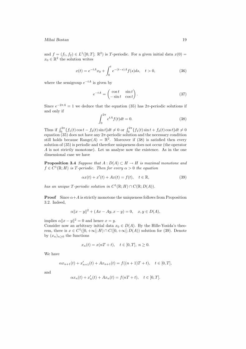
and f = (f1, f2) ∈ L1(]0, T [; R2) is T -periodic. For a given initial data x(0) =x0 ∈ R2 the solution writes

x(t) = e−tAx0 +∫ t

0

e−(t−s)Af(s)ds, t > 0, (36)

where the semigroup e−tA is given by

e−tA =(

cos t sin t− sin t cos t

). (37)

Since e−2πA = 1 we deduce that the equation (35) has 2π-periodic solutions ifand only if ∫ 2π

0

etAf(t)dt = 0. (38)

Thus if∫ 2π

0f1(t) cos t− f2(t) sin tdt 6= 0 or

∫ 2π

0f1(t) sin t+ f2(t) cos tdt 6= 0

equation (35) does not have any 2π-periodic solution and the necessary conditionstill holds because Range(A) = R

2. Moreover if (38) is satisfied then everysolution of (35) is periodic and therefore uniqueness does not occur (the operatorA is not strictly monotone). Let us analyse now the existence. As in the onedimensional case we have

Proposition 3.4 Suppose that A : D(A) ⊂ H → H is maximal monotone andf ∈ C1(R;H) is T -periodic. Then for every α > 0 the equation

αx(t) + x′(t) +Ax(t) = f(t), t ∈ R, (39)

has an unique T -periodic solution in C1(R;H) ∩ C(R;D(A)).

Proof Since α+A is strictly monotone the uniqueness follows from Proposition3.2. Indeed,

α‖x− y‖2 + (Ax−Ay, x− y) = 0, x, y ∈ D(A),

implies α‖x− y‖2 = 0 and hence x = y.Consider now an arbitrary initial data x0 ∈ D(A). By the Hille-Yosida’s theo-rem, there is x ∈ C1([0,+∞[;H) ∩ C([0,+∞[;D(A)) solution for (39). Denoteby (xn)n≥0 the functions

xn(t) = x(nT + t), t ∈ [0, T ], n ≥ 0.

We have

αxn+1(t) + x′n+1(t) +Axn+1(t) = f((n+ 1)T + t), t ∈ [0, T ],

andαxn(t) + x′n(t) +Axn(t) = f(nT + t), t ∈ [0, T ].


Since f is T -periodic, after usual computations we get

α‖xn+1(t)− xn(t)‖2 +12d

dt‖xn+1(t)− xn(t)‖2

+(Axn+1(t)−Axn(t), xn+1(t)− xn(t)) = 0, t ∈ [0, T ].

Taking into account that A is monotone we deduce

‖xn+1(t)− xn(t)‖ ≤ e−αt‖xn+1(0)− xn(0)‖, t ∈ [0, T ],

and hence

‖xn+1(0)− xn(0)‖ = ‖xn(T )− xn−1(T )‖≤ e−αT ‖xn(0)− xn−1(0)‖≤ e−2αT ‖xn−1(0)− xn−2(0)‖≤ ...

≤ e−nαT ‖x1(0)− x0(0)‖, n ≥ 0. (40)

Finally we get the estimate

‖xn+1(t)− xn(t)‖ ≤ e−α(nT+t)‖Sα(T ; 0, x0)− x0‖, t ∈ [0, T ], n ≥ 0.

Here Sα(t; 0, x0) represents the solution of (39) for the initial data x0. From theprevious estimate it is clear that (xn)n≥0 is convergent in C0([0, T ];H):

xn(t) = x0(t) +n−1∑k=0

(xk+1(t)− xk(t)), t ∈ [0, T ],

where

∥∥ n−1∑k=0

(xk+1(t)− xk(t))∥∥ ≤

n−1∑k=0

‖xk+1(t)− xk(t)‖

≤n−1∑k=0

e−α(kT+t)‖Sα(T ; 0, x0)− x0‖

≤ e−αt

1− e−αT‖Sα(T ; 0, x0)− x0‖.

Moreover ‖xn(t)‖ ≤ ‖Sα(t; 0, x0)‖ + 11−e−αT ‖Sα(T ; 0, x0) − x0‖. Denote by

xα the limit of (xn)n≥0 as n → ∞. We should note that without any otherhypothesis (xα)α>0 is not uniformly bounded in L∞(]0, T [;H). We have onlyestimate in O(1 + 1

α ),

‖xα‖L∞([0,T ];H) ≤ C(1 +

11− e−αT

)∼ O

(1 +

1α

).

The above estimate leads immediately to the following statement.

Mihai Bostan 21

Remark 3.5 The sequence (αxα)α>0 is uniformly bounded in L∞([0, T ];H).

Let us demonstrate that xα is T -periodic and solution for (39). Indeed,

xα(0) = limn→∞

xn(0) = limn→∞

xn−1(T ) = xα(T ).

Now let us show that (x′n)n≥0 is also uniformly bounded in L∞(]0, T [;H). Bytaking the difference between the equations (39) at the moments t and t+h wehave

α(x(t+h)−x(t))+x′(t+h)−x′(t)+Ax(t+h)−Ax(t) = f(t+h)−f(t), t < t+h.

Multiplying by x(t+ h)− x(t) we obtain

α‖x(t+h)−x(t)‖2 +12d

dt‖x(t+h)−x(t)‖2 ≤ ‖f(t+h)−f(t)‖·‖x(t+h)−x(t)‖,

which can be also rewritten as

12e2αt‖x(t+ h)− x(t)‖2 ≤

∫ t

0

eαs‖f(s+ h)− f(s)‖ · eαs‖x(s+ h)− x(s)‖ds

+12‖x(h)− x(0)‖2, t < t+ h.

By using Bellman’s lemma we conclude that

1h‖x(t+ h)− x(t)‖ ≤

∫ t

0

e−α(t−s) 1h‖f(s+ h)− f(s)‖ds

+e−αt1h‖x(h)− x(0)‖, 0 ≤ t < t+ h. (41)

By passing to the limit for h→ 0 the previous formula yields

‖x′(t)‖ ≤ e−αt‖x′(0)‖+∫ t

0

e−α(t−s)‖f ′(s)‖ds

≤ e−αt‖f(0)− αx0 −Ax0‖+1α

(1− e−αt)‖f ′‖L∞(]0,T [;H)

≤ ‖f(0)− αx0 −Ax0‖+1α‖f ′‖L∞(]0,T [;H) < +∞.

Therefore (x′n)n≥0 is uniformly bounded in L∞(]0, T [;H) since

‖x′n‖L∞(]0,T [;H) = ‖x′(nT + (·))‖L∞(]0,T [;H) ≤ ‖x′‖L∞([0,+∞[;H),

and thus we have x′n(t) yα(t), t ∈ [0, T ]. We can write

(xn(t), z) = (xn(0), z) +∫ t

0

(x′n(s), z)ds, z ∈ H, t ∈ [0, T ], n ≥ 0,


and by passing to the limit for n→∞ we deduce

(xα(t), z) = (xα(0), z) +∫ t

0

(yα(s), z)ds, z ∈ H, t ∈ [0, T ],

which is equivalent to

xα(t) = xα(0) +∫ t

0

yα(s)ds, t ∈ [0, T ].

Therefore xα is differentiable and x′α = yα. Finally we can write x′n(t) x′α(t),t ∈ [0, T ]. Let us show that xα is also solution for (39). We have

[xn(t), f(t)− αxn(t)− x′n(t)] ∈ A, n ≥ 0, t ∈ [0, T ].

Since xn(t) → xα(t), x′n(t) x′α(t) and A is maximal monotone we concludethat

[xα(t), f(t)− x′α(t)] ∈ A, t ∈ [0, T ], α > 0,

which means that xα(t) ∈ D(A) and Axα(t) = f(t)− x′α(t), t ∈ [0, T ].

Now we establish for the linear case the similar result stated in Proposition2.10. Before let us recall a standard result concerning maximal monotone oper-ators on Hilbert spaces

Proposition 3.6 Assume that A is a maximal monotone operator (linear ornot) and αuα + Auα = f , uα ∈ D(A), f ∈ H, α > 0. Then the followingstatements are equivalent:(i) f ∈ Range(A);(ii) (uα)α>0 is bounded in H. Moreover, in this case (uα)α>0 is convergent inH to the element of minimal norm in A−1f .

Proof it (i) → (ii) By the hypothesis there is u ∈ D(A) such that f = Au.After multiplication by uα − u we get

α(uα, uα − u) + (Auα −Au, uα − u) = 0, α > 0.

Taking into account that A is monotone we deduce

‖uα‖2 ≤ (uα, u) ≤ ‖uα‖ · ‖u‖, α > 0,

and hence ‖uα‖ ≤ ‖u‖, α > 0, u ∈ A−1f which implies that uα u0. We have[uα, f − αuα] ∈ A, α > 0 and since A is maximal monotone, by passing to thelimit for α→ 0 we deduce that [u0, f ] ∈ A, or u0 ∈ A−1f . Moreover

‖u0‖ = ‖w − limα→0

uα‖ ≤ lim infα→0

‖uα‖ ≤ lim supα→0

‖uα‖ ≤ ‖u‖, ∀u ∈ A−1f.

In particulat taking u = u0 ∈ A−1f we get

‖w − limα→0

uα‖ = limα→0‖uα‖,

Mihai Bostan 23

and hence, since any Hilbert space is strictly convex, by Mazur’s theorem wededuce that the convergence is strong

uα → u0 ∈ A−1f, α→ 0,

where ‖u0‖ = infu∈A−1f ‖u‖ = minu∈A−1f ‖u‖.(ii)→ (i) Conversely, suppose that (uα)α>0 is bounded in H. Therefore uα uin H. We have [uα, f − αuα] ∈ A, α > 0 and since A is maximal monotoneby passing to the limit for α → 0 we deduce that [u, f ] ∈ A or u ∈ D(A) andf = Au.

Theorem 3.7 Assume that A : D(A) ⊂ H → H is a linear maximal monotoneoperator on a compact Hilbert space H and f ∈ C1(R;H) is a T -periodic func-tion. Then the following statements are equivalent:(i) equation (33) has periodic solutions;(ii) the sequence of periodic solutions for (39) is bounded in C1(R;H). Moreoverin this case (xα)α>0 is convergent in C0(R;H) and the limit is also a T -periodicsolution for (33).

Proof (i) → (ii) Denote by x, xα the periodic solutions for (33) and (39). Bytaking the difference and after multiplication by xα(t)− x(t) we get:

α‖xα(t)−x(t)‖2 +12d

dt‖xα(t)−x(t)‖2 ≤ α‖x(t)‖ ·‖xα(t)−x(t)‖, t ∈ R. (42)

Finally, after integration and by using Bellman’s lemma, formula (42) yields

‖xα(t)− x(t)‖ ≤ e−αt‖xα(0)− x(0)‖+∫ t

0

αe−α(t−s)‖x(s)‖ds

≤ e−αt‖xα(0)− x(0)‖+ (1− e−αt)‖x‖L∞ , t ∈ R.

Since xα and x are T -periodic we can also write

‖xα(t)− x(t)‖ = ‖xα(nT + t)− x(nT + t)‖≤ e−α(nT+t)‖xα(0)− x(0)‖+ (1− e−α(nT+t))‖x‖L∞ .

By passing to the limit for n→∞ we obtain

‖xα − x‖L∞ ≤ ‖x‖L∞ , α > 0,

and hence‖xα‖L∞ ≤ 2‖x‖L∞ , α > 0.

Since A is linear we can write

α

h(xα(t+ h)− xα(t)) +

1h

(x′α(t+ h)− x′α(t)) +1hA(xα(t+ h)− xα(t))

=1h

(f(t+ h)− f(t)), t < t+ h, α > 0,


and for t < t+ h,

1h

(x′(t+ h)− x′(t)) +1hA(x(t+ h)− x(t)) =

1h

(f(t+ h)− f(t)).

For every h > 0 denote by yα,h, yh and gh the periodic functions:

yα,h(t) =1h

(xα(t+ h)− xα(t)), t ∈ R, α > 0,

yh(t) =1h

(x(t+ h)− x(t)), t ∈ R,

gh(t) =1h

(f(t+ h)− f(t)), t ∈ R,

and hence we have

αyα,h(t) + y′α,h(t) +Ayα,h(t) = gh(t), t ∈ R,y′h(t) +Ayh(t) = gh(t), t ∈ R.

By the same computations we get

‖yα,h(t)− yh(t)‖ ≤ e−αt‖yα,h(0)− yh(0)‖+∫ t

0

αe−α(t−s)‖yh(s)‖ds.

Now by passing to the limit for h→ 0 we deduce

‖x′α(t)− x′(t)‖ ≤ e−αt‖x′α(0)− x′(0)‖+∫ t

0

αe−α(t−s)‖x′(s)‖ds

≤ e−αt‖x′α(0)− x′(0)‖+ (1− e−αt)‖x′‖L∞ , t ∈ [0, T ].

By the periodicity we obtain as before that

‖x′α(t)− x′(t)‖ = ‖x′α(nT + t)− x′(nT + t)‖≤ e−α(nT+t)‖x′α(0)− x′(0)‖+ (1− e−α(nT+t))‖x′‖L∞ ,

and hence by passing to the limit for n→∞ we conclude that

‖x′α − x′‖L∞ ≤ ‖x′‖L∞ , α > 0.

Therefore, (x′α)α>0 is also uniformly bounded in L∞

‖x′α‖L∞ ≤ 2‖x′‖L∞ , α > 0.

Conversely, the implication (ii) → (i) follows by using Arzela-Ascoli’s theoremand by passing to the limit for α→ 0 in (39).

Let us continue the analysis of the previous example. The semigroup asso-ciated to the equation (39) is given by

e−t(α+A) = e−αte−tA = e−αt(

cos t, sin t− sin t, cos t

)t ∈ R, α > 0,

Mihai Bostan 25

and the periodic solution for equation (39) reads

xα(t) = (1− e−T (α+A))−1

∫ T

0

e−(T−s)(α+A)f(s)ds

+∫ t

0

e−(t−s)(α+A)f(s)ds

=1− e−T (α−A)

(1− e−αT cosT )2 + (e−αT sinT )2

∫ T

0


+∫ t

0

e−(t−s)(α+A)f(s)ds, t > 0, α > 0.

As we have seen, proving the existence of periodic solutions reduces to findinguniform L∞(]0, T [;H) estimates for (xα)α>0 and (x′α)α>0 . Since A is linearbounded operator (‖A‖L(H;H) = 1) we have

‖x′α‖L∞(]0,T [;H) = ‖f − αxα −Axα‖L∞(]0,T [;H)

≤ ‖f‖L∞(]0,T [;H) + (α+ ‖A‖L(H;H))‖xα‖L∞(]0,T [;H), α > 0,

and hence in this case it is sufficient to find only uniform L∞(]0, T [;H) estimatesfor (xα)α>0 or uniform estimates for (xα(0))α>0 in H.Case 1: T = 2nπ, n ≥ 0. We have

limα→0

xα(0) = limα→0

11− e−αT

∫ T

0

e−(T−s)(α+A)f(s)ds.

If∫ T

0e−(T−s)Af(s)ds 6= 0 , then (xα(0))α>0 is not bounded. In fact since

e−2nπA = 1 it is easy to check that equation (35) does not have any periodicsolution. If

∫ T0e−(T−s)Af(s)ds = 0 then every solution of (35) is T -periodic and

(xα(0))α>0 is convergent for α→ 0:

limα→0

xα(0) = limα→0

∫ T0

(e−α(T−s) − 1)e−(T−s)Af(s)ds1− e−αT

= −∫ T

0

T − sT

e−(T−s)Af(s)

=1T

∫ T

0

se−(T−s)Af(s).

Case 2: T 6= 2nπ for alln ≥ 0. In this case (1 − e−TA) is invertible and(xα(0))α>0 converges to x(0) where x is the unique T -periodic solution of (35):

limα→0

xα(0) = limα→0

(1− e−T (α+A))−1

∫ T

0


= (1− e−TA)−1

∫ T

0

e−(T−s)Af(s)ds

=1

2 sin(T2 )

∫ T

0

e−(T+π2 −s)Af(s)ds.


We state now our main result of existence in the linear and symmetric case.

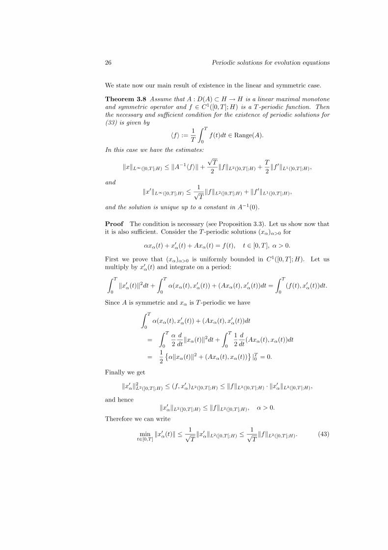
Theorem 3.8 Assume that A : D(A) ⊂ H → H is a linear maximal monotoneand symmetric operator and f ∈ C1([0, T ];H) is a T -periodic function. Thenthe necessary and sufficient condition for the existence of periodic solutions for(33) is given by

〈f〉 :=1T

∫ T

0

f(t)dt ∈ Range(A).

In this case we have the estimates:

‖x‖L∞(]0,T [;H) ≤ ‖A−1〈f〉‖+√T

2‖f‖L2(]0,T [;H) +

T

2‖f ′‖L1(]0,T [;H),

and‖x′‖L∞(]0,T [;H) ≤

1√T‖f‖L2(]0,T [;H) + ‖f ′‖L1(]0,T [;H),

and the solution is unique up to a constant in A−1(0).

Proof The condition is necessary (see Proposition 3.3). Let us show now thatit is also sufficient. Consider the T -periodic solutions (xα)α>0 for

αxα(t) + x′α(t) +Axα(t) = f(t), t ∈ [0, T ], α > 0.

First we prove that (xα)α>0 is uniformly bounded in C1([0, T ];H). Let usmultiply by x′α(t) and integrate on a period:∫ T

0

‖x′α(t)‖2dt+∫ T

0

α(xα(t), x′α(t)) + (Axα(t), x′α(t))dt =∫ T

0

(f(t), x′α(t))dt.

Since A is symmetric and xα is T -periodic we have∫ T

0

α(xα(t), x′α(t)) + (Axα(t), x′α(t))dt

=∫ T

0

α

2d

dt‖xα(t)‖2dt+

∫ T

0

12d

dt(Axα(t), xα(t))dt

=12α‖xα(t)‖2 + (Axα(t), xα(t))

|T0 = 0.

Finally we get

‖x′α‖2L2(]0,T [;H) ≤ (f, x′α)L2(]0,T [;H) ≤ ‖f‖L2(]0,T [;H) · ‖x′α‖L2(]0,T [;H),

and hence‖x′α‖L2(]0,T [;H) ≤ ‖f‖L2(]0,T [;H), α > 0.

Therefore we can write

mint∈[0,T ]

‖x′α(t)‖ ≤ 1√T‖x′α‖L2(]0,T [;H) ≤

1√T‖f‖L2(]0,T [;H). (43)

Mihai Bostan 27

As seen before, since A is linear we can write

α

h(xα(t+ h)− xα(t)) +

1h

(x′α(t+ h)− x′α(t))

+1hA(xα(t+ h)− xα(t)) =

1h

(f(t+ h)− f(t)),

and by standard calculations for s < t and h > 0, we get

1h‖xα(t+ h)− xα(t)‖

≤ e−α(t−s) 1h‖xα(s+ h)− xα(s)‖+

∫ t

s

e−α(t−τ) 1h‖f(τ + h)− f(t)‖dτ .

Passing to the limit for h→ 0 we deduce

‖x′α(t)‖ ≤ e−α(t−s)‖x′α(s)‖+∫ t

s

e−α(t−τ)‖f ′(τ)‖dτ

≤ ‖x′α(s)‖+∫ t

s

‖f ′(τ)‖dτ, s ≤ t, α > 0. (44)

From (43) and (44) we conclude that the functions (x′α)α>0 are uniformlybounded in L∞(]0, T [;H):

‖x′α‖L∞(]0,T [;H) ≤1√T‖f‖L2(]0,T [;H) + ‖f ′‖L1(]0,T [;H), α > 0.

As shown before, since A is linear and xα is T -periodic we have also

α〈xα〉+A〈xα〉 = 〈f〉. (45)

By the hypothesis there is x0 ∈ D(A) such that 〈f〉 = Ax0 and hence

‖〈xα〉‖ = ‖(α+A)−1〈f〉‖ = ‖(α+A)−1Ax0‖ ≤ ‖x0‖, α > 0.

Now it is easy to check that (xα)α>0 is uniformly bounded in L∞(]0, T [;H):

‖xα(t)− 〈xα〉‖ =∥∥∥ 1T

∫ T

0

(xα(t)− xα(s))ds∥∥∥

=∥∥∥ 1T

∫ T

0

∫ t

s

x′α(τ)dτds∥∥∥

≤√T

2‖f‖L2(]0,T [;H) +

T

2‖f ′‖L1(]0,T [;H),

and thus

‖xα‖L∞(]0,T [;H) ≤ ‖〈xα〉‖+√T

2‖f‖L2(]0,T [;H) +

T

2‖f ′‖L1(]0,T [;H)

≤ ‖x0‖+√T

2‖f‖L2(]0,T [;H) +

T

2‖f ′‖L1(]0,T [;H).


Now we can prove that (xα)α>0 is convergent in C1([0, T ];H). Indeed, bytaking the difference between the equations (39) written for α, β > 0, aftermultiplication by x′α(t)− x′β(t) and integration on [0, T ] we get∫ T

0

α(xα(t)− xβ(t), x′α(t)− x′β(t))

+‖x′α(t)− x′β(t)‖2 + (A(xα(t)− xβ(t)), x′α(t)− x′β(t))dt

= −(α− β)∫ T

0

(xβ(t), x′α(t)− x′β(t))dt.

Since A is symmetric, xα and xβ are T -periodic and uniformly bounded inL∞(]0, T [;H) we deduce that

‖x′α − x′β‖L2(]0,T [;H) ≤ |α− β| · supγ>0‖xγ‖L2(]0,T [;H),

or

‖x′α−x′β‖L∞(]0,T [;H) ≤|α− β|√

T·supγ>0‖xγ‖L2(]0,T [;H) + |α−β| ·sup

γ>0‖x′γ‖L1(]0,T [;H),

and therefore (x′α)α>0 converges in C([0, T ];H).We already know that (〈xα〉)α>0 = ((α+A)−1〈f〉)α>0 is bounded in H and

by the Proposition 3.6 it follows that (〈xα〉)α>0 is convergent to the element ofminimal norm in A−1〈f〉. We have

xα(t) = xα(0) +∫ t

0

x′α(s)ds, t ∈ R, α > 0.

By taking the average we deduce that xα(0) = 〈xα〉− <∫ t

0x′α(s)ds > and

therefore, since (x′α)α>0 is uniformly convergent, it follows that (xα(0))α>0 isalso convergent. Finally we conclude that (xα)α>0 is convergent in C1([0, T ];H)to the periodic solution x for (33) such that < x > is the element of minimalnorm in A−1〈f〉.

Before analyzing the periodic solution for the heat equation, following anidea of [7], let us state the following proposition.

Proposition 3.9 Assume that A : D(A) ⊂ H → H is a linear maximal mono-tone and symmetric operator and f ∈ C1([0, T ];H) is a T -periodic function.Then for every x0 ∈ D(A) we have

limt→∞

1T

(x(t+ T ; 0, x0)− x(t; 0, x0)) = 〈f〉 − ProjR(A)〈f〉, (46)

where x(·; 0, x0) represents the solution of (33) with the initial data x0 and R(A)is the range of A.

Remark 3.10 A being maximal monotone, A−1 is also maximal monotone andtherefore D(A−1) = R(A) is convex.

Mihai Bostan 29

Proof of Proposition 3.9. Consider x0 ∈ D(A) and denote by x(·) thecorresponding solution. By integration on [t, t+ T ] we get

1T

(x(t+ T )− x(t)) +A( 1T

∫ t+T

t

x(s)ds)

= 〈f〉. (47)

For each α > 0 consider xα ∈ D(A) such that αxα + Axα = 〈f〉. Denoting byy(·) the function y(t) = 1

T

∫ t+Tt

x(s)ds, t ≥ 0, equation (47) writes

y′(t) +Ay(t) = αxα +Axα, t ≥ 0, α > 0.

Let us search for y of the form y1 + y2 where

y′1(t) +Ay1(t) = αxα, t ≥ 0,

with the initial condition y1(0) = 0 and

y′2(t) +Ay2(t) = Axα, t ≥ 0, (48)

with the initial condition y2(0) = y(0) = 1T

∫ T0x(t)dt. We are interested on the

asymptotic behaviour of Ay(t) = Ay1(t) +Ay2(t) for large t. We have

y1(t) = e−tAy1(0) +∫ t

0

e−(t−s)Aαxαds

=∫ t

0

e−(t−s)Aαxαds,

and therefore,

Ay1(t) =∫ t

0

Ae−(t−s)Aαxαds = e−(t−s)Aαxα

∣∣∣t0

= (1− e−tA)αxα.

By the other hand, after multiplication of (48) by y′2(t) = (y2(t)− xα)′ we get

‖y′2(t)‖2 + (A(y2(t)− xα), (y2(t)− xα)′) = 0, t ≥ 0.

Since A is symmetric, after integration on [0, t] we obtain∫ t

0

‖y′2(s)‖2ds+12

(A(y2(t)− xα), y2(t)− xα) =12

(A(y2(0)− xα), y2(0)− xα),

and therefore, by the monotony of A it follows that∫ ∞0

‖y′2(t)‖2dt ≤ 12

(A(y2(0)− xα), y2(0)− xα).


Thus limt→∞ y′2(t) = 0 and by passing to the limit in (48) we deduce thatlimt→∞Ay2(t) = limt→∞(Axα − y′2(t)) = Axα. Finally we find that

limt→∞

1T

(x(t+ T )− x(t))− e−tAαxα

= limt→∞y′(t)− e−tAαxα

= limt→∞〈f〉 −Ay(t)− e−tAαxα

= limt→∞〈f〉 −Ay1(t)−Ay2(t)− e−tAαxα

= 〈f〉 − αxα −Axα = 0, α > 0. (49)

Now let us put yα = Axα and observe that yα + αA−1yα = Axα + αxα =〈f〉, α > 0. Therefore,

limα0

yα = limα0

(1 + αA−1)−1〈f〉

= limα0

JA−1

α 〈f〉

= ProjD(A−1)

〈f〉= Proj

R(A)〈f〉,

and it follows that

limα0

αxα = limα0

(〈f〉 −Axα) = limα0

(〈f〉 − yα) = 〈f〉 − ProjR(A)〈f〉.

Since Graph(A) is closed and [αxα, αyα] = [αxα, A(αxα)] ∈ A, α > 0, bypassing to the limit for α 0 we deduce that 〈f〉 − Proj

R(A)〈f〉 ∈ D(A) and

A(〈f〉 − ProjR(A)〈f〉) = 0. It is easy to see that we can pass to the limit for

α 0 in (49). Indeed, for ε > 0 let us consider αε > 0 such that ‖ limα0 αxα−αεxαε‖ < ε

2 . We have∥∥ 1T

(x(t+ T )− x(t))− e−tA limα0

αxα∥∥

≤∥∥ 1T

(x(t+ T )− x(t))− e−tAαεxαε∥∥+

∥∥e−tAαεxαε − e−tA limα0

αxα∥∥

≤∥∥ 1T

(x(t+ T )− x(t))− e−tAαεxαε∥∥+ ‖αεxαε − lim

α0αxα‖

≤ ε

2+ε

2= ε, t ≥ t(αε,

ε

2) = t(ε),

and thus

limt→∞ 1T

(x(t+ T )− x(t))− e−tA(〈f〉 − ProjR(A)〈f〉) = 0.

But e−tA(〈f〉 − ProjR(A)〈f〉) does not depend on t ≥ 0:

d

dte−tA(〈f〉 − Proj

R(A)〈f〉) = −Ae−tA(〈f〉 − Proj

R(A)〈f〉)

= −e−tAA(〈f〉 − ProjR(A)〈f〉) = 0,

Mihai Bostan 31

and thus the previous formula reads

limt→∞

1T

(x(t+ T )− x(t)) = 〈f〉 − ProjR(A)〈f〉.

Remark 3.11 Under the same hypothesis as above we can easily check that

infx0∈D(A)

‖x(T ; 0, x0)− x0‖T

= ‖〈f〉 − ProjR(A)〈f〉‖ = dist(〈f〉, R(A)).

3.3 Periodic solutions for the heat equation

Let Ω ⊂ Rd, d ≥ 1, be an open bounded set with ∂Ω ∈ C2. Consider the heatequation

∂u

∂t(t, x)−∆u(t, x) = f(t, x), (t, x) ∈ R× Ω, (50)

with the Dirichlet boundary condition

u(t, x) = g(t, x), (t, x) ∈ R× ∂Ω, (51)

or the Neumann boundary condition

∂u

∂n(t, x) = g(t, x), (t, x) ∈ R× ∂Ω, (52)

where we denote by n(x) the outward normal in x ∈ ∂Ω.

Theorem 3.12 Assume that f ∈ C1(R;L2(Ω)) is T -periodic and g(t, x) =∂u0∂n (t, x), (t, x) ∈ R×∂Ω where u0 ∈ C1(R;H2(Ω))∩C2(R;L2(Ω)) is T -periodic.

Then the heat problem (50), (52) has T -periodic solutions u ∈ C(R;H2(Ω)) ∩C1(R;L2(Ω)) if and only if∫

∂Ω

∫ T

0

g(t, x)dtdσ +∫

Ω

∫ T

0

f(t, x)dtdx = 0.

In this case the periodic solutions satisfies the estimates

‖u′ − u′0‖L∞([0,T ];L2(Ω)) ≤ 1√T‖f − u′0 + ∆u0‖L2(]0,T [;L2(Ω))

+ ‖f ′ − u′′0 + ∆u′0‖L1(]0,T [;L2(Ω)), (53)

and the solution is unique up to a constant.

Proof Let us search for solutions u = u0 + v where

∂v

∂t(t, x)−∆v(t, x) = f(t, x)− ∂u0

∂t(t, x) + ∆u0(t, x), (t, x) ∈ R× Ω, (54)

and∂v

∂n(t, x) = g(t, x)− ∂u0

∂n(t, x) = 0, (t, x) ∈ R× ∂Ω. (55)


Consider the operator AN : D(AN ) ⊂ L2(Ω)→ L2(Ω) given as

ANv = −∆v

with domain

D(AN ) =v ∈ H2(Ω) :

∂v

∂n(x) = 0, ∀ x ∈ ∂Ω

.

The operator AN is linear monotone:

(ANv, v) = −∫

Ω

∆v(x)v(x)dx

= −∫∂Ω

∂v

∂n(x)v(x)dσ +

∫Ω

‖∇v(x)‖2dx

=∫

Ω

‖∇v(x)‖2dx ≥ 0, ∀ v ∈ D(AN ). (56)

Since the equation λv − ∆v = f has unique solution in D(AN ) for every f ∈L2(Ω), λ > 0 it follows that AN is maximal (see [6]). Moreover, it is symmetric

(ANv1, v2) =∫

Ω

∇v1(x) · ∇v2(x)dx = (v1, ANv2), ∀ v1, v2 ∈ D(AN ).

Note that by the hypothesis the second member in (54) f −u′0 +∆u0 belongs toC1(R;L2(Ω)). Therefore the Theorem 3.8 applies and hence the problem (54),(55) has periodic solutions if and only if there is w ∈ D(AN ) such that

−∆w =1T

∫ T

0

f(t)− du0

dt(t) + ∆u0(t)dt.

Since u0 is T -periodic we have∫ T

0du0dt (t)dt = 0 and thus w + 1

T

∫ T0u0(t)dt is

solution for the elliptic problem

−∆(w +

1T

∫ T

0

u0(t)dt)

=1T

∫ T

0

f(t)dt = F,

with the boundary condition

∂

∂n

(w +

1T

∫ T

0

u0(t)dt)

=∂w

∂n+

1T

∫ T

0

∂u0

∂n(t)dt

=1T

∫ T

0

g(t)dt = G.

As known from the general theory of partial differential equations (see [6]) thisproblem has solution if and only if

∫∂ΩG(x)dσ +

∫ΩF (x)dx = 0 or∫

∂Ω

∫ T

0

g(t, x)dtdσ +∫

Ω

∫ T

0

f(t, x)dtdx = 0.

The estimate (53) follows from Theorem 3.8.For the heat equation with Dirichlet boundary condition we have the follow-

ing existence result.

Mihai Bostan 33

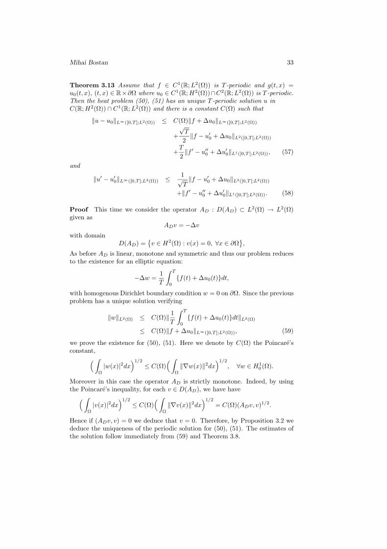
Theorem 3.13 Assume that f ∈ C1(R;L2(Ω)) is T -periodic and g(t, x) =u0(t, x), (t, x) ∈ R×∂Ω where u0 ∈ C1(R;H2(Ω))∩C2(R;L2(Ω)) is T -periodic.Then the heat problem (50), (51) has an unique T -periodic solution u inC(R;H2(Ω)) ∩ C1(R;L2(Ω)) and there is a constant C(Ω) such that

‖u− u0‖L∞([0,T ];L2(Ω)) ≤ C(Ω)‖f + ∆u0‖L∞([0,T ];L2(Ω))

+√T

2‖f − u′0 + ∆u0‖L2(]0,T [;L2(Ω))

+T

2‖f ′ − u′′0 + ∆u′0‖L1(]0,T [;L2(Ω)), (57)

and

‖u′ − u′0‖L∞([0,T ];L2(Ω)) ≤ 1√T‖f − u′0 + ∆u0‖L2(]0,T [;L2(Ω))

+‖f ′ − u′′0 + ∆u′0‖L1(]0,T [;L2(Ω)). (58)

Proof This time we consider the operator AD : D(AD) ⊂ L2(Ω) → L2(Ω)given as

ADv = −∆v

with domainD(AD) =

v ∈ H2(Ω) : v(x) = 0, ∀x ∈ ∂Ω

,

As before AD is linear, monotone and symmetric and thus our problem reducesto the existence for an elliptic equation:

−∆w =1T

∫ T

0

f(t) + ∆u0(t)dt,

with homogenous Dirichlet boundary condition w = 0 on ∂Ω. Since the previousproblem has a unique solution verifying

‖w‖L2(Ω) ≤ C(Ω)‖ 1T

∫ T

0

f(t) + ∆u0(t)dt‖L2(Ω)

≤ C(Ω)‖f + ∆u0‖L∞([0,T ];L2(Ω)), (59)

we prove the existence for (50), (51). Here we denote by C(Ω) the Poincare’sconstant,(∫

Ω

|w(x)|2dx)1/2

≤ C(Ω)(∫

Ω

‖∇w(x)‖2dx)1/2

, ∀w ∈ H10 (Ω).

Moreover in this case the operator AD is strictly monotone. Indeed, by usingthe Poincare’s inequality, for each v ∈ D(AD), we have have(∫

Ω

|v(x)|2dx)1/2

≤ C(Ω)(∫

Ω

‖∇v(x)‖2dx)1/2

= C(Ω)(ADv, v)1/2.

Hence if (ADv, v) = 0 we deduce that v = 0. Therefore, by Proposition 3.2 wededuce the uniqueness of the periodic solution for (50), (51). The estimates ofthe solution follow immediately from (59) and Theorem 3.8.


3.4 Non-linear case

Throughout this section we will consider evolution equations associated to sub-differential operators. Let ϕ : H →]−∞,+∞] be a lower-semicontinuous properconvex function on a real Hilbert space H. Denote by ∂ϕ ⊂ H × H the sub-differential of ϕ,

∂ϕ(x) =y ∈ H; ϕ(x)− ϕ(u) ≤ (y, x− u), ∀u ∈ H

, (60)

and denote by D(ϕ) the effective domain of ϕ:

D(ϕ) =x ∈ H; ϕ(x) < +∞

.

Under the previous assumptions on ϕ we recall that A = ∂ϕ is maximal mono-tone in H ×H and D(A) = D(ϕ). Consider the equation

x′(t) + ∂ϕx(t) 3 f(t), 0 < t < T. (61)

We say that x is solution for (61) if x ∈ C([0, T ];H), x is absolutely continuouson every compact of ]0, T [ (and therefore a.e. differentiable on ]0, T [) and sat-isfies x(t) ∈ D(∂ϕ) a.e. on ]0, T [ and x′(t) + ∂ϕx(t) 3 f(t) a.e. on ]0, T [. Wehave the following main result [1]

Theorem 3.14 Let f be given in L2(]0, T [;H) and x0 ∈ D(∂ϕ). Then theCauchy problem (61) with the initial condition x(0) = x0 has a unique solutionx ∈ C([0, T ];H) which satisfies:

x ∈W 1,2(]δ, T [;H) ∀ 0 < δ < T,√t · x′ ∈ L2(]0, T [;H), ϕ x ∈ L1(0, T ).

Moreover, if x0 ∈ D(ϕ) then

x′ ∈ L2(]0, T [;H), ϕ x ∈ L∞(0, T ).

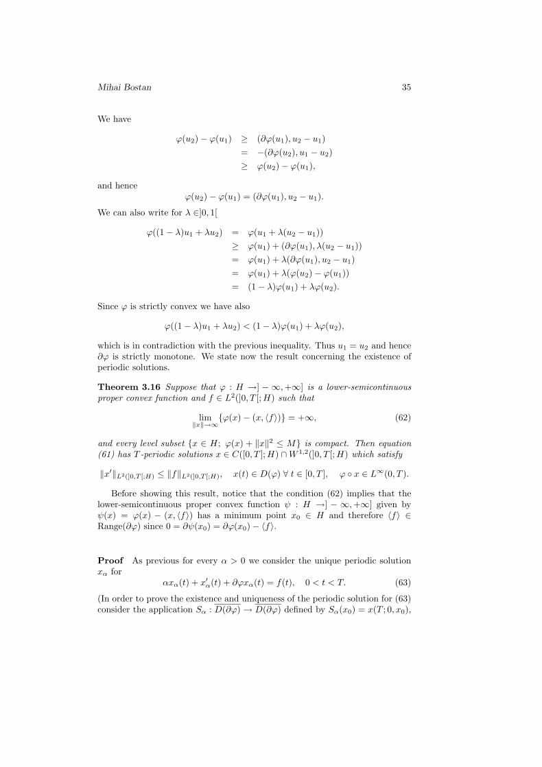
We are interested in finding sufficient conditions on A = ∂ϕ and f such thatequation (61) has unique T -periodic solution, i.e. x(0) = x(T ). Obviously, ifsuch a solution exists, by periodicity we deduce that it is absolutely continuouson [0, T ] and belongs to W 1,2(]0, T [;H). It is well known that if ϕ is strictlyconvex then ∂ϕ is strictly monotone and therefore the uniqueness holds

Proposition 3.15 Assume that ϕ : H →]−∞,+∞] is a lower-semicontinuousproper, strictly convex function. Then equation (61) has at most one periodicsolution.

Proof By using Proposition 3.2 it is sufficient to prove that ∂ϕ is strictlymonotone. Suppose that there are u1, u2 ∈ D(∂ϕ), u1 6= u2 such that

(∂ϕ(u1)− ∂ϕ(u2), u1 − u2) = 0.

Mihai Bostan 35

We have

ϕ(u2)− ϕ(u1) ≥ (∂ϕ(u1), u2 − u1)= −(∂ϕ(u2), u1 − u2)≥ ϕ(u2)− ϕ(u1),

and henceϕ(u2)− ϕ(u1) = (∂ϕ(u1), u2 − u1).

We can also write for λ ∈]0, 1[

ϕ((1− λ)u1 + λu2) = ϕ(u1 + λ(u2 − u1))≥ ϕ(u1) + (∂ϕ(u1), λ(u2 − u1))= ϕ(u1) + λ(∂ϕ(u1), u2 − u1)= ϕ(u1) + λ(ϕ(u2)− ϕ(u1))= (1− λ)ϕ(u1) + λϕ(u2).

Since ϕ is strictly convex we have also

ϕ((1− λ)u1 + λu2) < (1− λ)ϕ(u1) + λϕ(u2),

which is in contradiction with the previous inequality. Thus u1 = u2 and hence∂ϕ is strictly monotone. We state now the result concerning the existence ofperiodic solutions.

Theorem 3.16 Suppose that ϕ : H →] − ∞,+∞] is a lower-semicontinuousproper convex function and f ∈ L2(]0, T [;H) such that

lim‖x‖→∞

ϕ(x)− (x, 〈f〉) = +∞, (62)

and every level subset x ∈ H; ϕ(x) + ‖x‖2 ≤ M is compact. Then equation(61) has T -periodic solutions x ∈ C([0, T ];H) ∩W 1,2(]0, T [;H) which satisfy

‖x′‖L2(]0,T [;H) ≤ ‖f‖L2(]0,T [;H), x(t) ∈ D(ϕ) ∀ t ∈ [0, T ], ϕ x ∈ L∞(0, T ).

Before showing this result, notice that the condition (62) implies that thelower-semicontinuous proper convex function ψ : H →] − ∞,+∞] given byψ(x) = ϕ(x) − (x, 〈f〉) has a minimum point x0 ∈ H and therefore 〈f〉 ∈Range(∂ϕ) since 0 = ∂ψ(x0) = ∂ϕ(x0)− 〈f〉.

Proof As previous for every α > 0 we consider the unique periodic solutionxα for

αxα(t) + x′α(t) + ∂ϕxα(t) = f(t), 0 < t < T. (63)

(In order to prove the existence and uniqueness of the periodic solution for (63)consider the application Sα : D(∂ϕ)→ D(∂ϕ) defined by Sα(x0) = x(T ; 0, x0),


where x(·; 0, x0) denote the unique solution of (63) with the initial condition x0

and apply the Banach’s fixed point theorem. By the previous theorem it followsthat the periodic solution xα is absolutely continuous on [0, T ] and belongs toC([0, T ];H)∩W 1,2(]0, T [;H)). First of all we will show that (x′α)α>0 is uniformlybounded in L2(]0, T [;H). Indeed, after multiplication by x′α(t) we obtain∫ T

0

‖x′α(t)‖2dt+∫ T

0

α(xα(t), x′α(t))+(∂ϕxα(t), x′α(t))dt =∫ T

0

(f(t), x′α(t))dt.

Since xα is T -periodic we deduce that∫ T

0

α(xα(t), x′α(t)) + (∂ϕxα(t), x′α(t))dt

=∫ T

0

d

dtα

2‖xα(t)‖2 + ϕ(xα(t))dt

=α

2‖xα(t)‖2 + ϕ(xα(t))|T0 = 0. (64)

Therefore, ‖x′α‖2L2(]0,T [;H) ≤ (f, x′α)L2(]0,T [;H) and thus

‖x′α‖L2(]0,T [;H) ≤ ‖f‖L2(]0,T [;H), α > 0.

Before estimate (xα)α>0, let us check that (αxα)α>0 is bounded. By takingx0 ∈ D(∂ϕ), after standard calculation we find that

‖xα(t)−x0‖ ≤ e−αt‖xα(0)−x0‖+∫ t

0

e−α(t−s)‖f(s)−αx0− ∂ϕ(x0)‖ ds. (65)

Since xα is T -periodic we can write

‖xα(t)− x0‖ = limn→∞

‖xα(nT + t)− x0‖

≤ limn→∞

e−α(nT+t)‖xα(0)− x0‖

+∫ nT+t

0

e−α(nT+t−s)‖f(s)− αx0 − ∂ϕ(x0)‖ ds

≤ 1α‖αx0 + ∂ϕ(x0)‖+ lim

n→∞

∫ nT+t

0

e−α(nT+t−s)‖f(s)‖ ds

≤ 1α‖αx0 + ∂ϕ(x0)‖

+ limn→∞

[1 + e−αt(e−α(n−1)T + · · ·+ e−αT + 1)

]· ‖f‖L1

=

1α‖αx0 + ∂ϕ(x0)‖+

(1 +

e−αt

1− e−αT)· ‖f‖L1(]0,T [;H)

≤ C1(x0, T, ‖f‖L2(]0,T [;H))(1 +

1α

), 0 ≤ t ≤ T, α > 0.

Mihai Bostan 37

It follows that α‖xα(t)‖ ≤ C2(x0, T, ‖f‖L2(]0,T [;H)), 0 ≤ t ≤ T , 0 < α < 1. Nowwe can estimate xα, α > 0. After multiplication by xα(t) and integration on[0, T ] we obtain

∫ T

0

α‖xα(t)‖2dt+∫ T

0

(∂ϕ(xα(t)), xα(t))dt =∫ T

0

(f(t), xα(t))dt. (66)

We have

ϕ(x0) ≥ ϕ(xα(t)) + (∂ϕ(xα(t)), x0 − xα(t)), t ∈ [0, T ], α > 0.

Thus we deduce that for α > 0,

∫ T

0

(∂ϕ(xα(t)), xα(t))dt ≥∫ T

0

ϕ(xα(t))dt+∫ T

0

(∂ϕ(xα(t)), x0)− ϕ(x0)dt.

On the other hand for 0 < α < 1,

∫ T

0

(∂ϕ(xα(t)), x0) dt =∫ T

0

(f(t)− αxα(t)− x′α(t), x0) dt

=(∫ T

0

f(t) dt, x0

)−∫ T

0

(αxα(t), x0) dt

≥ −C3(x0, T, ‖f‖L2(]0,T [;H)).

Therefore,

∫ T

0

(∂ϕ(xα(t)), xα(t))dt ≥∫ T

0

ϕ(xα(t))dt− C4(x0, T, ‖f‖L2(]0,T [;H)). (67)

Combining (66) and (67) we deduce that

∫ T

0

ϕ(xα(t))dt ≤ C4 +∫ T

0

(∂ϕ(xα(t)), xα(t))dt

= C4 +∫ T

0

(f(t), xα(t))dt−∫ T

0

α‖xα(t)‖2dt

≤ C4 +∫ T

0

(f(t), xα(t))dt, 0 < α < 1. (68)


On the other hand we have∫ T

0

(f(t), xα(t))dt

=∫ T

0

(f(t)− 〈f〉, xα(t))dt+(∫ T

0

xα(t)dt, 〈f〉)

=∫ T

0

(f(t)− 〈f〉, xα(0) +∫ t

0

x′α(s) ds)dt+ T (〈xα〉, 〈f〉)

=∫ T

0

(f(t)− 〈f〉,∫ t

0

x′α(s) ds)dt+ T (〈xα〉, 〈f〉)

≤∫ T

0

‖f(t)− 〈f〉‖ ·(∫ t

0

‖x′α(s)‖2 ds)1/2

· t1/2 dt+ T (〈xα〉, 〈f〉)

≤ ‖f − 〈f〉‖L2(]0,T [;H) · ‖f‖L2(]0,T [;H) ·T√2

+ T (〈xα〉, 〈f〉).

Finally we deduce that∫ T

0

ϕ(xα(t))− (xα(t), 〈f〉) dt ≤ C5(x0, T, ‖f‖L2(]0,T [;H)), 0 < α < 1, (69)

and thus there is tα ∈ [0, T ] such that

ϕ(xα(t))− (xα(t), 〈f〉) ≤ C5

T, 0 < α < 1. (70)

From Hypothesis (62) we get that (xα(tα))0<α<1 is bounded and therefore from(65), for t ∈ [tα, tα + T ],

‖xα(t)− x0‖ ≤ e−α(t−tα)‖xα(tα)− x0‖+∫ t

tα

e−α(t−s)‖f(s)− αx0 − ∂ϕ(x0)‖ ds.

we deduce that (xα)0<α<1 is bounded in L∞(]0, T [;H) and that there is x ∈L∞(]0, T [;H) such that xα(t) x(t) when α goes to 0 for t ∈ [0, T ]. Moreover,from (70) it follows that (ϕ(xα(tα)))0<α<1 is bounded from above and we deducethat

ϕ(xα(t)) = ϕ(xα(tα)) +∫ t

tα

(∂ϕ(xα(s)), x′α(s)) ds

≤ ϕ(xα(tα)) +∫ t

tα

(f(s)− αxα(s)− x′α(s), x′α(s)) ds

≤ C6(x0, T, ‖f‖L2(]0,T [;H)), 0 < α < 1.

On the other hand, by writing ϕ(xα(t)) ≥ ϕ(x0) + (∂ϕ(x0), xα(t)−x0), 0 ≤ t ≤T , α > 0 we deduce that ϕ(xα(t)) is also bounded from below so that finally(ϕ xα)0<α<1 is bounded in L∞(]0, T [;H).

Mihai Bostan 39

Now, using the second hypothesis of the theorem (every level subset is com-pact) we deduce that xα(0)→ x(0) when α goes to 0 (at least for a subsequenceαn 0). In fact we can easily check that xα converges uniformly to x on [0, T ]since

‖xα(t)− xβ(t)‖ ≤ ‖xα(0)− xβ(0)‖+ |α− β| · T · sup0<γ<1

‖xγ‖L∞(]0,T [;H),

for 0 ≤ t ≤ T , 0 < α, β < 1. Now, since limα0 dxα/dt = dx/dt in thesense of H-valued vectorial distribution on ]0, T [ and (x′α)α>0 is bounded inL2(]0, T [;H) it follows that x′ belongs to L2(]0, T [;H) and in particular x isabsolutely continuous on every compact of ]0, T [ and therefore a.e. differentiableon ]0, T [.

To complete the proof we need to show that x(t) ∈ D(ϕ) a.e. on ]0, T [ andx′(t) + ∂ϕx(t) 3 f(t) a.e. on ]0, T [. For arbitrarily [u, v] ∈ ∂ϕ we have

12e2αt‖xα(t)−u‖2 ≤ 1

2e2αs‖xα(s)−u‖2 +

∫ t

s

e2ατ (f(τ)−αu− v, xα(τ)−u) dτ,

with 0 ≤ s ≤ t ≤ T , α > 0. Passing to the limit for α 0 we get

12‖x(t)− u‖2 ≤ 1

2‖x(s)− u‖2 +

∫ t

s

(f(τ)− v, x(τ)− u) dτ, 0 ≤ s ≤ t ≤ T.

Thus

(x(t)−x(s), x(s)−u) ≤ 12‖x(t)−u‖2− 1

2‖x(s)−u‖2 ≤

∫ t

s

(f(τ)−v, x(τ)−u) dτ,

for 0 ≤ s ≤ t ≤ T . Since x is a.e. differentiable on ]0, T [ we find that

(x′(t), x(t)− u) = limst

1t− s

(x(t)− x(s), x(s)− u)

≤ limst

1t− s

∫ t

s

(f(τ)− v, x(τ)− u) dτ

= (f(t)− v, x(t)− u), a.e. t ∈]0, T [, ∀ [u, v] ∈ ∂ϕ.

Finally, since ∂ϕ is maximal monotone and (f(t)−x′(t)−v, x(t)−u) ≥ 0 for all[u, v] ∈ ∂ϕ we deduce that x(t) ∈ D(∂ϕ) a.e. on ]0, T [ and x′(t) +∂ϕx(t) 3 f(t)a.e. on ]0, T [. Since ϕ is lower-semicontinuous we also have

ϕ(x(t)) ≤ limα0

inf ϕ(xα(t)) ≤ limα0

inf ‖ϕ xα‖L∞ ≤ sup0<γ<1

‖ϕ xγ‖L∞ .

As previous, by writing

ϕ(x(t)) ≥ ϕ(x0) + (∂ϕ(x0), x(t)− x0)≥ ϕ(x0)− ‖∂ϕ(x0)‖ · (‖x0‖+ lim

α0inf ‖xα(t)‖)

≥ ϕ(x0)− ‖∂ϕ(x0)‖ · (‖x0‖+ sup0<γ<1

‖xγ‖L∞), 0 ≤ t ≤ T,

we deduce finally that ϕ x ∈ L∞(0, T ).


Remark 3.17 If dimH < +∞ then the level subsets x ∈ H ; ϕ(x) + ‖x‖2 ≤M are compact as bounded sets.

Remark 3.18 Assume that ϕ : H →] − ∞,+∞] is a lower-semicontinuousproper convex function such that Range(∂ϕ) = H which is equivalent to

lim‖x‖→∞

ϕ(x)− (x, y) = +∞, ∀y ∈ H,

see [4], pp.41. In particular, by taking y = 〈f〉 we deduce that the hypothesis(62) is verified.

Remark 3.19 Assume that ϕ is coercive

lim‖x‖→∞

(∂ϕ(x), x− x0)‖x‖

= +∞, ∀x0 ∈ D(ϕ),

which is equivalent to lim‖x‖→∞ϕ(x)‖x‖ = +∞ (see [4], pp.42). Then Range(ϕ) =

H because the previous condition is satisfied: lim‖x‖→∞ϕ(x)− (x, y) = +∞,for all y ∈ H and therefore (62) is verified.

Theorem 3.20 Suppose that ϕ : H →] − ∞,+∞] is a lower-semicontinuousproper convex function and f ∈W 1,1(]0, T [;H) such that

lim‖x‖→∞

ϕ(x)− (x, 〈f〉) = +∞, (71)

and every level subset x ∈ H; ϕ(x) + ‖x‖2 ≤ M is compact. Then equation(61) has T -periodic solutions x ∈ C([0, T ];H) ∩W 1,∞(]0, T [;H) which satisfy

x(t) ∈ D(∂ϕ), ∀ t ∈ [0, T ],d+

dtx(t) + (∂ϕx(t)− f(t)) = 0, ∀ t ∈ [0, T ],

where (∂ϕ− f) denote the minimal section of ∂ϕ− f .

Proof Since W 1,1(]0, T [;H) ⊂ L2(]0, T [;H) the previous theorem applies.Consider x ∈ C([0, T ];H)∩W 1,2(]0, T [;H) a T -periodic solution for (61). Since‖x′‖L2(]0,T [;H) ≤ ‖f‖L2(]0,T [;H) it follows that there is t? ∈]0, T [ such that x isdifferentiable in t? and ‖x′(t?)‖ ≤ 1√

T‖f‖L2(]0,T [;H). By standard calculation

we find that:

‖ 1h

(x(t+ h)− x(t))‖ ≤ ‖ 1h

(x(t? + h)− x(t?))‖+∫ t

t?‖ 1h

(f(τ + h)− f(τ)‖ dτ,

and therefore sup0≤t≤T, h>0 ‖ 1h (x(t + h) − x(t))‖ ≤ C which implies that x ∈

W 1,∞(]0, T [;H). Making use of the inequality

1h

(x(t+h)−x(t), x(t)−u) ≤ 1h

∫ t+h

t

(f(τ)−v, x(τ)−u) dτ, 0 ≤ t < t+h ≤ T,

Mihai Bostan 41

which holds for every [u, v] ∈ ∂ϕ we deduce that x(t) ∈ D(∂ϕ) for all t ∈[0, T ] and the weak closure of the set 1

h (x(t + h) − x(t)), h > 0 belongs tof(t)− ∂ϕx(t), ∀t ∈ [0, T ]. On the other hand by writing

‖x(t+ h)− u‖ ≤ ‖x(t)− u‖+∫ t+h

t

‖f(τ)− v‖ dτ, 0 ≤ t < t+ h ≤ T,

for u = x(t) and v ∈ ∂ϕx(t) we find that

‖(∂ϕx(t)− f(t))‖ ≤ ‖w − limh0

1h

(x(t+ h)− x(t))‖

≤ lim suph0

‖ 1h

(x(t+ h)− x(t))‖

≤ ‖(∂ϕx(t)− f(t))‖.

This shows that limh01h (x(t + h) − x(t)) = d+

dt x(t) exists for every t ∈ [0, T ]and coincides with −(∂ϕx(t)− f(t)).

References

[1] V. Barbu, Nonlinear Semigroups and Differential Equations in BanachSpaces, Noordhoff (1976).

[2] M. Bostan, Solutions periodiques des equations d’evolution, C. R. Acad.Sci. Paris, Ser. I Math. t.332, pp. 1-4, Equations derivees partielles, (2001).

[3] M. Bostan, Almost periodic solutions for evolution equations, article inpreparation.

[4] H. Brezis, Operateurs maximaux monotones et semi-groupes de contractionsdans les espaces de Hilbert, Noth-Holland, Lecture Notes no. 5 (1972).

[5] H. Brezis, A Haraux, Image d’une somme d’operateurs monotones et ap-plications, Israel J. Math. 23 (1976), 2, pp. 165-186.

[6] H. Brezis, Analyse fonctionnelle, Masson, (1998).

[7] A. Haraux, Equations d’evolution non lineaires: solutions borneesperiodiques, Ann. Inst. Fourier 28 (1978), 2, pp. 202-220.

Mihai Bostan

Universite de Franche-Comte16 route de Gray F-25030Besancon Cedex, [email protected]

Documents

Periodic solutions for evolution equations