Embed Size (px)
Citation preview
Asymptotic Analysis for Schrödinger Hamiltoniansvia Birkho�-Gustavson Normal Form
Kaoutar Ghomaria, Bekkai Messirdib and San V�u Ngo.cc
aDepartment of Mathematics and Computer Sciences, ENP-Oran, BP
1523 El'Mnaouar 31000, Algeria.
E-mail adress: [email protected], [email protected] of Mathematics, University of Oran Es-Senia, BP 1524 El'Mnaouar
31000, Algeria.
E-mail adress: [email protected] Research Institute IRMAR, University of Rennes 1 and Insti-
tut Universitaire de France, 263, Avenue du Général Leclerc, 35042 Rennes
CEDEX, France.
E-mail adress: [email protected]
AbstractThis article reviews the Birkho�-Gustavson normal form theorem (BGNF)
near an equilibrium point of a quantum Hamiltonian. The BGNF process is
thereafter used to investigate the spectrum of Schrödinger operators in the
1:1, 1:2 and 1:3 resonances. A computer program is proposed to compute the
coe�cients of the BGNF up to any order.
Key words and phrases : Birkho� Normal Form, Harmonic oscillator,
Bargmann representation, Resonances, Fermi resonance.
1 Introduction
The topic under consideration in this paper is the computation of theBirkho�-Gustavson normal form and its application to the calculationof the quantum mechanical spectra of Schrödinger operators.
An old and important problem in quantum mechanics is the investi-gation of the discrete spectrum of selfajoint operators. There are severalclassical methods for the numerical computation of eigenvalues. Many ofthem amount to writing a �nite dimensional approximation of the oper-ator in a suitable basis, and performing numerical diagonalization. It iswell known that the choice of basis is delicate and crucial : a bad choicecan easily lead to very poor numerical accuracy. With this respect, whenquantum Birkho�-Gustavson normal form can be used, they generallygive excellent results.
(0)2000 MSC : 58K50, 81S10, 81Q10
1

The theory of normal forms is one of the theories that allow us toanalyse the spectrum of a Hamiltonian near an equilibrium position of asmooth potential. This mathematical theory has a rather long history,dating back to Poincaré, and has received much attention. The �rst rig-orous set-up, in the framework of Hamiltonian classical mechanics, wasgiven in [4] by Birkho� in the case where the quadratic approximationof the hamiltonian is a sum of harmonic oscillators with non-resonantfrequencies; it has been extended then to the resonant case by Gustavson[8].
Several physicists in the 1980's have started to think about a quan-tum version of the Birkho�-Gustavson normal form (BGNF). The mainidea is based on two steps. The �rst one is the classical step: �nd thenormal form by canonical transformations of the coordinates and mo-menta; the second one is to quantize this normal form. The �rst step iswell studied and now considered rather straightforward, but the quan-tization of the normal form addresses the fundamental question of howto quantize a classical problem in which the coordinates and momentadoes not appear in a simple manner. Even in the Birkho�-Gustavsonprocedure, it is not clear a priori which quantization scheme would bethe most natural. One can consult for this the works of M. K. Ali [1]where he makes the comparison between various notions of quantization.
The BGNF played an important role in classical mechanics in per-mitting, for example, to investigate the stability of elliptic trajectories[6]. It has been applied with remarkable success in molecular physicsand became a very powerful tool, attested by the excellent numericalresults obtained in [12] and more recently in [9] and [10].
On the mathematics side, the development of sophisticated tools forperforming functional analysis in phase space, starting with pseudodif-ferential operators, microlocal and semiclassical analysis, has been veryimportant for a better understanding and more accurate applicationsof quantum normal forms. The BGNF for pseudodi�erential operatorsnear a non-degenerate minimum of the symbol has been used by severalauthors, see for example the works of Bambusi [2] about semiclassicalnormal forms; also the article by Sjöstrand [11] that treats the non-resonant case and the one by Charles and Vu Ngoc [5] for the resonantcase.
The goal of this article is to exhibit explicit calculations of the BGNFin some simple resonant situations which can be encountered in physicalmodels, like small molecules. This article is organized as follows :
In section 2, we �rst start with recalling the procedure that leadsSchrödinger operators P = −h2
2∆ + V (x), when V is a smooth poten-
tial, to their Birkho�-Gustavson normal form P = H2 + K, where K
2

commutes with the harmonic oscillator H2. In this procedure, the quan-tization and normalization steps are combined at each order, contraryto, for instance, [11], where quantization was applied only after the fullclassical normal form was obtained.
In section 3, we calculate the BGNF in the 1:1, 1:2 and 1:3 resonances.We introduce the creation and annihilation operators and Bargmanntransform and �nally we inject everything in Bargmann space. Thisallows an easy computation of the principal coe�cients of the normalform in the three cases.
In section 4, one of the main goals of this work, we calculate thespectrum σ(P ) of the operator P thanks to the analysis of the spectrumσ(K) of the restriction of K to the eigenspaces of H2. Since H2 and Kcommute, one �nally gets the spectrum of P , up to a small error term,simply by adding to σ(K) the corresponding explicit eigenvalue of H2.
All the results in sections 3 and 4 were carefully done by hand. How-ever, it is clear that the computation of higher order approximations,involving higher order terms of the Birkho�-Gustavson normal form, be-comes very soon intractable for human abilities. On the other hand, thenormal form algorithm is clear enough to be implemented on a computer.We propose in section 5 a program, whose code is available on-line(1),which is based on the non-commutative calculus of Weyl algebra andthat can easily give the quantum Birkho�-Gustavson normal form of agiven Hamiltonian up to any order.
2 BGNF theorem
We recall the Birkho�-Gustavson normal form theorem, BGNF, whichis fundamental for this work.
Consider on L2 (Rn) the Schrödinger operator
P = −~2
2∆ + V (y) (1)
where ~ > 0, ∆ is the n−dimensional Laplacian and V is a smooth realpotential on Rn, having a non-degenerate global minimum at 0 whichwe shall call here the origin. By a linear unitary change of variables inlocal coordinates near 0, one can assume that the hessian matrix V ′′ (0)is diagonal, let (ν2
1, ..., ν2n) be its eigenvalues, with νj > 0. The rescaling
xj =√νjyj transforms P into a perturbation of the harmonic oscillator
H2 :P = H2 +W (x) (2)
(1)http://blogperso.univ-rennes1.fr/san.vu-ngoc/public/divers/
birkhoff_0.4.tgz
3

with H2 =n∑j=1
νj2
(−~2 ∂2
∂x2j+ x2
j
), where W (x) is a smooth potential of
order O( |x|3) at the origin.We work with the space
E =C[[x, ξ, ~]] = C[[x1, ..., xn, ξ1, ..., ξn, ~]]
x= (x1, ..., xn) , ξ = (ξ1, ..., ξn)
of formal power series of (2n + 1) variables with complex coe�cients,where the degree of the monomial xαξβ~` is de�ned to be |α|+ |β|+ 2`,α, β ∈ Nn, ` ∈ N.
Let DN be the �nite dimensional vector space spanned by monomialsof degree N and ON the subspace of E consisting of formal series whoseco�cients of degree < N vanish. Let A ∈ E , we shall need in this articlethe Weyl bracket [., .]W de�ned on polynomials by :
[f, g]W = σW (f g − gf) , for all f, g ∈ E (3)
where f and g are the (formal) Weyl quantizations of symbols f andg, and σW is the complete Weyl symbol map. The Weyl quantizationof a polynomial in (x, ξ) consists in replacing xj by the multiplicationby xj operator, and ξj by
~i∂∂xj
, and averaging all the possible orderings
of the variables x an ξ. Thus, for instance, the Weyl quantization ofx1ξ1 is the di�erential operator ~
i(x1
∂∂x1
+ 12). Then the bracket de�ned
in (3) can be computed recursively according to the rules [xj, xk]W =[ξj, ξk
]W
= [~, xj]W =[~, ξj
]W
= 0 and[ξj, xk
]W
= ~iδj,k, where δj,k is
the Kronecker index.The formal quantum Birkho� normal form can be expressed as fol-
lows :
Theorem 1 (BGNF Theorem) Let H2 ∈ D2 and L ∈ O3, then there
exists A ∈ O3 and K ∈ O3 such that :
ei~−1adA (H2 + L) = H2 +K (BGNF)
where K = K3 +K4 + ..., with Kj ∈ Dj commutes with H2 :
[H2, K]W = 0
Moreover if H2 and L have real coe�cients then A and K can be chosento have real coe�cients as well.
4

Notice that the sum
ei~−1adA (H2 + L) =
∞∑l=0
1
`!
(i
~adA
)`(H2 + L) (4)
is usually not convergent in the analytic sense, even if L comes froman analytic function, but it is always convergent in the topology of Ebecause the map B 7→ i
~adA(B) = i~ [A,B]W sends ON into ON+1
The equation (BGNF) is called the Birkho�-Gustavson normal formof the operator P at the origin.
3 Birkho�-Gustavson normal form in the 1:1, 1:2and 1:3 resonances
3.1 Creation and annihilation operators
Let Xj denote the operator of multiplication by xj and Yj the operator∂∂xj
in L2 (Rn) .
aj (~) =1√2~
(Xj + ~Yj) =1√2~
(xj + ~∂
∂xj) (5)
bj (~) =1√2~
(Xj − ~Yj) =1√2~
(xj − ~∂
∂xj)
are respectively called the operators of creation and annihilation inL2 (Rn) .
The operators aj (~) and bj (~) formally satisfy :
a∗j (~) = bj (~) , b∗j (~) = aj (~)
[aj (~) , bk (~)] = δjk , [aj (~) , ak (~)] = 0 , [bj (~) , bk (~)] = 0
While rewriting H2 according to aj (~) and bj (~) , one gets,
H2 = ~n∑j=1
νj(aj (~) bj (~)− 1
2) (6)
3.2 Bargmann representation
In this paragraph, we recall some standard results concerning the spaceBF of Bargmann-Fock (simply called the Bargmann space) and theBargmann transform. For more details one can consult [3].
Let us consider the space
5
BF =
ϕ (z) holomorphic function on Cn ;
∫Cn
|ϕ (z)|2 dµn (z) < +∞
where dµn (z) is the Gaussian measure de�ned by dµn (z) = π−ne−
|z|2~ dnz =
π−ne−|z|2~ dnxdny. BF is a Hilbert space when it is equipped with the nat-
ural inner product :
< f, g >=
∫Cn
f (z) g (z)dµn (z)
Theorem 2 ([3]) There exists a unitary mapping TB from L2 (Rn) toBF de�ned by
(TBf) (z) =2n/4
(2π~)3n/4
∫Rn
f (x) e−12(z2+x2)+
√2xzπ−ndnx (7)
TB is called the Bargmann transform.
We recall that H2 is essentially self-adjoint with a discrete spectrumσ(H2) which consists of the eigenvalues:
λN = ~(< ν, α > +
|ν|2
)= ~
(N +
|ν|2
), N =< ν, α >=
n∑j=1
νjαj
ν = (ν1, ..., νn), α = (α1, ..., αn) ∈ Nn and |ν| =n∑j=1
νj.
The associated eigenspaces areHN = vect {ψα (x) ; < ν, α >= N} whereψα (x) = e−
12x2Pα (x) are the standard Hermite functions (here Pα(x) is
a polynomial of degree |α|) which constitute an orthonormal hilbertianbasis {ψα (x)}α of L2 (Rn).
Then we have the following theorem :
Theorem 3 The isometry TB sends the functions {ψα (x)}α∈Nn to the
functions{
zα√α!
}α∈Nn
which constitute an orthonormal hilbertian basis of
BF .
In the Bargmann representation of quantum mechanics, physicalstates are mapped into entire functions of a complex variable z, whereasthe creation and annihilation operators play the role of di�erentiationand multiplication with respect to z, respectively.
6

Proposition 4 If we denote by Zj the operator of multiplication by zj
and Dj the operator ∂∂zj
on BF , then :
TB (aj (~))T−1B = Dj and TB (bj (~))T−1
B = Zj (8)
The Bargmann transform of the harmonic oscillator is given by
HB2 = TB
(H2
)T−1B = ~
n∑j=1
νj(zj∂
∂zj+
1
2) (9)
and the eigenspace associated to the eigenvalue λN is the linear subspacespanned by the functions zα1√
α1!zα2√α2!
such that ν1α1 + ν2α2 = N :
HBN = vect
{ϕα = ϕ(α1,α2) =
zα1
√α1!
zα2
√α2!
; ν1α1 + ν2α2 = N
}3.3 BGNF in the 1:1 resonance
Consider the following harmonic oscillator
H2 =1
2
(−~2 ∂
2
∂x21
+ x21
)+
1
2
(−~2 ∂
2
∂x22
+ x22
)with symbol
H2 = |z1|2 + |z2|2
where zj = 1√2
(xj + iξj
); j = 1, 2.
The Bargmann transform of H2 is given by
HB2 = TB
(H2
)T−1B = ~
(z1
∂
∂z1
+ z2∂
∂z2
+ 1
)Suppose now we are in the situation of the BGNF theorem (cf. equa-
tion (2)) : we want to understand the spectrum of an operator of the
form H2+L, where L is a perturbation term of order at least 3. From thetheorem, it is enough to study the spectrum of the normalized pertur-bation K (see [5]). The crucial question is therefore to compute the �rstnon-trivial term of the symbol K. Throughout the paper, when K is aformal series in E , we use the notation Kj to denote the homogeneouspart of degree j, and K(N) := K0 +K1 + · · ·+KN .
Since [H2, K3]W = 0 and thus {H2, K3} = 0, we have
K3 =∑
2`+|β|+|γ|=3
c(3)αβ~
`zαzβ such that < ν, β − α >= 0.
7

In other words, K3 is a linear combination of order 3 monomials ~`zαzβsuch that < ν, β − α >= 0.
The condition of 1:1 resonance, ν1 = ν2 = 1, is expressed by
< ν, β − α >= 0⇔ α1 + α2 = β1 + β2 (res 1:1)
where α = (α1, α2), β = (β1, β2) ∈ N2.
We notice that no monomial exists in D3 verifying at the same time|α|+ |β| = 3 and the resonance relation (res 1 : 1). This means K3 = 0.Thus we need to calculate K4, as a linear combination of monomialszα1
1 zα22 z
β11 z
β22 of order 4. We check that the couples α = (α1, α2) and
β = (β1, β2) which verify at the same time |α|+|β| = 4 and the resonancerelation (res 1 : 1) are :
α= β = (1, 1) , α = β = (2, 0) , α = β = (0, 2) ,
α= (2, 0) and β = (0, 2) , α = (0, 2) and β = (2, 0)
Thus K4 is generated by the monomials :
|z1|2 |z2|2 , |z1|4 , |z2|4 , z21z
22 , z
21z
22 , ~2
Since K is real, one can write
K4 = λ1 |z1|4 + λ2 |z2|4 + λ3 |z1|2 |z2|2 + λ4 Re(z2
1z22
)+ λ5~2 (10)
Evaluation of coe�cients λj :By the BGNF, the order 4 perturbation W4 turns into a new term
K4 which we will obtain as the projection onto the kernel of adH2 of theterm
W4 +i
2~[A3,W3]W , (11)
where A3 is de�ned by the relation
W3 =i
~adH2 (A3) . (12)
Indeed, applying the theorem 1 of Birkho�-Gustavson to H2 + W =H2 + W3 + W4 + ..., we obtain polynomials A3 ∈ D3 and K3 ∈ D3 suchas
ei~−1adA3 (H2 +W3 +O4) = H2 +K3 +O4 (13)
where K3 and H2 commute. We have
(13)⇔ H2 +W3 +i
~[A3, H2]W +O4 = H2 +K3 +O4.
8

SinceD3 = ker
(i~−1adH2
)⊕ Im
(i~−1adH2
), (14)
we may splitW3 = W3,1 + i~ [H2,W3,2]W whereW3,1 ∈ D3 commutes with
H2, and W3,2 ∈ D3. Therefore K3 = W3,1 and we can set A3 = W3,2;however, in the 1 : 1 resonance, ker (i~−1adH2) ∩ D3 = {0}, hence K3 =W1,3 = 0, and therefore A3 is de�ned by the relation (12).
Now, let A3 =∑
|α|+|β|=3
aα,βzαzβ andW3 =
∑|α|+|β|=3
cα,βzαzβ, then (12)
gives:
∑|α|+|β|=3
cα,βzαzβ =
i
~adH2
( ∑|α|+|β|=3
aα,βzαzβ
)=i
~∑
|α|+|β|=3
h < ν, β − α > aα,βzαzβ
from whereaα,β = −i cα,β
< ν, β − α >(15)
and from the 1 : 1 resonance relation we obtain
aα,β = −i cα,ββ1 + β2 − α1 − α2
, ∀α, β ∈ N2 ; |α|+ |β| = 3
It remains to �nd K4; since K3 = 0, the normal form writes
ei~−1ad(A3+A4) (H2 +W3 +W4 +O5) = H2 +K4 +O5 (16)
with [K4, H2] = 0. We have
ei~−1ad(A3+A4) (H2 +W3 +W4 +O5) = H2 +W3 +W4 +
i
~[A3, H2]W +
i
~[A4, H2]W
+i
~[A3,W3]W +
1
2!
(i
~
)2
[A3, [A3, H2]W ]W +O5
= H2 +W4 +i
~[A3,W3] +
i
2~
[A3,
i
~[A3, H2]
]+O5
because from (12), we have, i~ [A3, H2]W = − i
~ [H2, A3]W = −W3. So
(16)⇔ W4 +i
~[A4, H2]W +
i
~[A3,W3]W +
i
2~
[A3,
i
~[A3, H2]W
]W
+O5 = R4 +O5
⇔ W4 +i
~[A4, H2]W +
i
~[A3,W3]W −
i
2~[A3,W3]W +O5 = R4 +O5
⇔ W4 +i
~[A4, H2]W +
i
2~[A3,W3]W +O5 = K4 +O5
9

and therefore K4 must be the projection onto D4∩ker (i~−1adH2), in thesplitting (14), of the term
W4 +i
2~[A3,W3]W . (17)
In order to compute this projection, we express W3 in terms of the moreconvenient complex variables : zj = 1√
2
(xj + iξj
), so xj = 1√
2(zj + zj),
and we get, by Taylor expansion:
W3 =1
2√
2.3!
[∂3W (0)
∂x31
(z1 + z1)3 +∂3W (0)
∂x32
(z2 + z2)3
+ 3∂3W (0)
∂x21∂x2
(z1 + z1)2 (z2 + z2) + 3∂3W (0)
∂x1∂x22
(z1 + z1) (z2 + z2)2
]=
1
2√
2.3!
[∂3W (0)
∂x31
(z3
1 + 3z21 z1 + 3z1z
21 + z3
1
)+∂3W (0)
∂x32
(z3
2 + 3z22 z2 + 3z2z
22 + z3
2
)+3
∂3V (0)
∂x21∂x2
(z2
1z2 + z21 z2 + z2
1z2 + z21 z2 + 2z1z2z1 + 2z1z1z2
)+ 3
∂3V (0)
∂x1∂x22
(z2
2z1 + z22 z1 + z2
2z1 + z22 z1 + 2z2z1z2 + 2z2z2z1
)].
By the relation (15) we get
A3 =−i 1
2√
2.3!
[∂3W (0)
∂x31
(−1
3z3
1 − 3z21 z1 + 3z1z
21 +
1
3z3
1
)]+∂3W (0)
∂x32
(−1
3z3
2 − 3z22 z2 + 3z2z
22 +
1
3z3
2
)]+3
∂3W (0)
∂x21∂x2
(−1
3z2
1z2 − z21 z2 + z2
1z2 +1
3z2
1 z2 − 2z1z2z1 + 2z1z1z2
)+ 3
∂3W (0)
∂x1∂x22
(−1
3z2
2z1 − z22 z1 + z2
2z1 +1
3z2
2 z1 − 2z2z1z2 + 2z2z2z1
)]Now, we must calculate i
2~ [A3,W3]W . By the Moyal Formula:
i
2~[A3,W3]W =
1
2{A3,W3} −
~2
233!Π3 (A3,W3) +O5 (18)
where we use the bidi�erential operator Π(f, g) := fΠg given by
{f, g} = fΠg =n∑j=1
∂f
∂ξj
∂g
∂xj− ∂f
∂xj
∂g
∂ξj= −if
(←−∂
∂z
−→∂
∂z−←−∂
∂z
−→∂
∂z
)g
(19)
10

and
Π3 = i
[ ←−∂3
∂z3
−→∂3
∂z3− 3
←−∂2
∂z2
−→∂2
∂z2
←−∂
∂z
−→∂
∂z+ 3
←−∂
∂z
−→∂
∂z
←−∂2
∂z2
−→∂2
∂z2−←−∂3
∂z3
−→∂3
∂z3
](20)
= in∑j=1
←−∂3
∂z3j
−→∂3
∂z3j
− 3
←−∂3
∂z2j∂zj
−→∂3
∂z2j∂zj
+ 3
←−∂3
∂zj∂z2j
−→∂3
∂zj∂z2j
−←−∂3
∂z3j
−→∂3
∂z3j
Since A3 and W3 are in function of zαzβ, we can compute the Poissonbrackets using the following nice formula :
Lemma 5 ∀α, β, α′, β′ ∈ Nn:{zαzβ, zα
′zβ′}
= −izα+α′ zβ+β′n∑j=1
∣∣∣∣αj βjα′j β′j
∣∣∣∣ 1
zj zj(21)
Particular cases:{zα, zβ
}= 0 ;
{zα, zβ
}= 0 ;
{zα, zβ
}= −izαzβ
n∑j=1
αjβj1
zj zj.
Proof.{zαzβ, zα
′zβ′}
=−in∑j=1
∂zα11 ...zαnn z
β11 ...z
β11
∂zj
∂zα′11 ...z
α′nn z
β′11 ...z
β′11
∂zj
−∂zα11 ...zαnn z
β11 ...z
β11
∂zj
∂zα′11 ...z
α′nn z
β′11 ...z
β′11
∂zj
=−in∑j=1
βjα′jzα+α′−ej zβ+β′−ej − αjβ′jzα+α′−ej zβ+β′−ej
=−in∑j=1
(βjα
′j − αjβ′j
)zα+α′−ej zβ+β′−ej
which gives the result.After a long but straightforward calculation by hand and via this last
lemma, we arrive to gather all monomials of 12{A3,W3}, that are in K4,
11

and we obtain:
−1
2
(1
3!2√
2
)2[
60
{(∂3W (0)
∂x31
)2
+
(∂3W (0)
∂x21∂x2
)2}|z1|4
+60
{(∂3W (0)
∂x32
)2
+
(∂3W (0)
∂x22∂x1
)2}|z2|4
+
{72
[(∂3W (0)
∂x31
)(∂3W (0)
∂x21∂x2
)+
(∂3W (0)
∂x32
)(∂3W (0)
∂x22∂x1
)+(
∂3W (0)
∂x31
)(∂3W (0)
∂x22∂x1
)+
(∂3W (0)
∂x32
)(∂3W (0)
∂x21∂x2
)]+96
[(∂3W (0)
∂x21∂x2
)2
+
(∂3W (0)
∂x22∂x1
)2]}|z1|2 |z2|2
−3
{(∂3W (0)
∂x31
)(∂3W (0)
∂x21∂x2
)+
(∂3W (0)
∂x32
)(∂3W (0)
∂x22∂x1
)+
(∂3W (0)
∂x31
)(∂3W (0)
∂x22∂x1
)+
(∂3W (0)
∂x32
)(∂3W (0)
∂x21∂x2
)}Re(z2
1z22
)]and the second term of (18) is simply
− ~2
233!Π3 (A3,W3) =
1
233!.192
(1
2√
2.3!
)2[(
∂3W (0)
∂x31
)2
+
(∂3W (0)
∂x32
)2]~2
=1
72
[(∂3W (0)
∂x31
)2
+
(∂3W (0)
∂x32
)2]~2
Let's now, look for all monomials of W4 that should belong to K4.We have
W4 (x1, x2) =1
4!
(∂4W (0)
∂x41
x41 +
∂4W (0)
∂x42
x42 + 4
∂4W (0)
∂x31∂x2
x31x2
+ 4∂4W (0)
∂x32∂x1
x32x1 + 6
∂4W (0)
∂x21∂x
22
x21x
22
)We know from (10) that only the monomials x4
1, x42 and x
21x
22 inW4 (x1, x2)
may contribute to K4.
12

Now, if we let xj = 1√2
(zj + zj) , then:
x41 =
1
4(z1 + z1)4 =
1
4(z4
1 + 4z21 |z1|2 + 6 |z1|4︸ ︷︷ ︸
in K4
+ 4z21 |z1|2 + z4
1)
x42 =
1
4(z2 + z2)4 =
1
4(z4
2 + 4z22 |z2|2 + 6 |z2|4︸ ︷︷ ︸
in K4
+ 4z22 |z2|2 + z4
2)
x21x
22 =
1
4(z1 + z1)2 (z2 + z2)2
=1
4
z21z
22 + z2
1z22︸︷︷︸
in K4
+ 2z21 |z2|2 + z2
1z22︸︷︷︸
in K4
+ z21z
22
+ 2z21 |z2|2 + 2z2
2 |z1|2 + 2 |z1|2 z22 + 4|z1|2 |z2|2︸ ︷︷ ︸
in K4
from where, we get the other part of the terms of K4, that is:
1
16
∂4W (0)
∂x41
|z1|4+1
16
∂4W (0)
∂x42
|z2|4+1
4
∂4W (0)
∂x21∂x
22
|z1|2 |z2|2+1
8
∂4W (0)
∂x21∂x
22
Re(z2
1z22
)�nally we gather all terms that are in K4, and we obtain the coe�cientswe were looking for:
Theorem 6 The quantum Birkho�-Gustavson normal form of the Schrödingerhamiltonian in 1 : 1 resonance H2 +W is equal to H2 +K4 +O5 with
K4 = λ1 |z1|4 + λ2 |z2|4 + λ3 |z1|2 |z2|2 + λ4 Re(z2
1z22
)+ λ5~2,
13

where
λ1 =1
16
∂4W (0)
∂x41
− 1
2
(1
3!2√
2
)2
60
{(∂3W (0)
∂x31
)2
+
(∂3W (0)
∂x21∂x2
)2}
λ2 =1
16
∂4W (0)
∂x42
− 1
2
(1
3!2√
2
)2
60
{(∂3W (0)
∂x32
)2
+
(∂3W (0)
∂x22∂x1
)2}
λ3 =1
4
∂4W (0)
∂x21∂x
22
+ 72
[(∂3W (0)
∂x31
)(∂3W (0)
∂x21∂x2
)+
(∂3W (0)
∂x32
)(∂3W (0)
∂x22∂x1
)+
(∂3W (0)
∂x31
)(∂3W (0)
∂x22∂x1
)+
(∂3W (0)
∂x32
)(∂3W (0)
∂x21∂x2
)+96
(∂3W (0)
∂x21∂x2
)2
+
(∂3W (0)
∂x22∂x1
)2]
λ4 =1
8
∂4W (0)
∂x21∂x
22
− 3
[(∂3W (0)
∂x31
)(∂3W (0)
∂x21∂x2
)+
(∂3W (0)
∂x32
)(∂3W (0)
∂x22∂x1
)+
(∂3W (0)
∂x31
)(∂3W (0)
∂x22∂x1
)+
(∂3W (0)
∂x32
)(∂3W (0)
∂x21∂x2
)]λ5 =
1
72
[(∂3W (0)
∂x31
)2
+
(∂3W (0)
∂x32
)2]
The Weyl quantization of K4 gives a concrete representation of thisnormal form as a polynomial di�erential operator :
K4 =λ1
(x4
1 + ~4 ∂4
∂x41
− 2~2x21
∂2
∂x21
− 4~2x1∂
∂x1
− ~2
)+λ2
(x4
2 + ~4 ∂4
∂x42
− 2~2x22
∂2
∂x22
− 4~2x2∂
∂x2
− ~2
)+λ3
(x2
1x22 − ~2x2
1
∂2
∂x21
− ~2x22
∂2
∂x22
+ ~4 ∂2
∂x21
∂2
∂x22
)(22)
+λ4
[x2
1x22 + ~2x2
1
∂2
∂x22
+ ~2x22
∂2
∂x21
+ ~4 ∂2
∂x21
∂2
∂x22
− 4~2x1x2∂
∂x1
∂
∂x2
+ 2~2x1∂
∂x1
+ 2~2x2∂
∂x2
+ ~2
]+λ5~2
14

Using the creation and annihilation operators we get:
K4 = 2~2λ1
[a2
1 (~) b21 (~) + b2
1 (~) a21 (~)− 1
]+2~2λ2
[a2
2 (~) b22 (~) b2
2 (~) a22 (~)− 1
]+2~2λ (3a1 (~) b1 (~) a2 (~) b2 (~) (23)
+ b1 (~) a1 (~) b2 (~) a2 (~)− 1
2
)+2~2λ4[a2
1 (~) b22 (~) + a2
2 (~) b21 (~)])
+λ5~2
and by using Bargmann representation, we get
KB4 =TB
(K4
)T−1B = 2~2
[λ1
(1 + 4z1
∂
∂z1
+ 2z21
∂2
∂z21
)+λ2
(1 + 4z2
∂
∂z2
+ 2z22
∂2
∂z22
)+λ3
(1 + z1
∂
∂z1
+ z2∂
∂z2
+ 2z1z2∂2
∂z1∂z2
)+λ4
(z2
1
∂2
∂z22
+ z22
∂2
∂z21
)]+λ5~2
= 2~2
(2λ1z
21
∂2
∂z21
+ 2λ2z22
∂2
∂z22
+ 2λ3z1z2∂2
∂z1∂z2
+ λ4
(z2
1
∂2
∂z22
+ z22
∂2
∂z21
)+ (4λ1 + λ3) z1
∂
∂z1
+ (4λ2 + λ3) z2∂
∂z2
+
(λ1 + λ2 + λ3 +
λ5
2
))(24)
3.4 BGNF in the 1:2 resonance (Fermi resonance)
Let
H2 =1
2
(−~2 ∂
2
∂x21
+ x21
)+
(−~2 ∂
2
∂x22
+ x22
)with symbol
H2 = |z1|2 + 2 |z2|2
where zj = 1√2
(xj + iξj
); j = 1, 2.
The Bargmann transform of H2 is given by
HB2 = TB
(H2
)T−1B = ~
(z1
∂
∂z1
+ 2z2∂
∂z2
+3
2
)Since [H2, K3]W = 0, and thus {H2, K3} = 0, it is su�cient to calculate
K3 =∑
2`+|β|+|γ|=3
c(3)αβ~
`zαzβ
15

such that < ν, β − α >= 0.The condition of 1:2 resonance, ν1 = 1, ν2 = 2, is expressed by
< ν, β − α >= 0⇔ α1 + 2α2 = β1 + 2β2 (res 1:2)
where α = (α1, α2),β = (β1, β2) ∈ N2.To obtain K3, it is necessary to look for all monomials of order 3 thatsatisfy the Fermi resonance relation (res 1 : 2).The couples α = (α1, α2) and β = (β1, β2) which verify at the same time|α|+ |β| = 3 and the resonance relation (res 1 : 2) are :
α= (0, 1) and β = (2, 0)
α= (2, 0) and β = (0, 1)
Thus, K3 is generated by the monomials
z2z21 , z
21z2
Since K is real, we can write
K3 = µRe(z21z2) =
µ
2(z2z
21 + z2
1z2), µ ∈ R (25)
Evaluation of coe�cient µ :The term of third degree in Taylor series of W near the origine is
W3 (x1, x2) =1
3!
[∂3W (0)
∂x31
x31 +
∂3W (0)
∂x32
x32 + 3
∂3W (0)
∂x21∂x2
x21x2 + 3
∂3W (0)
∂x22∂x1
x22x1
]where W (x1, x2) =
∑j>3
Wj(x1, x2) given in formula (2).
If we put xj = 1√2
(zj + zj) ,We remark that, only the coe�cient of x21x2
in W3 (x1, x2) corresponds to the coe�cient of K3, because:
x21x2 =
1
2√
2
z21z2 + z2
1z2 + z21z2︸ ︷︷ ︸
in K3
+ z21z2 + 2 |z1|2 z2 + 2 |z1|2 z2
we obtain, the term in K3 :
1
2.
1
2√
2
∂3W (0)
∂x21∂x2
(z21z2 + z2
1z2) =1
2√
2
∂3W (0)
∂x21∂x2
Re(z21z2)
Theorem 7 The quantum Birkho�-Gustavson normal form of the Schrödingerhamiltonian in 1 : 2 resonance H2 +W is equal to H2 +K3 +O4 with
K3 = µRe(z21z2)
where
µ =1
2√
2
∂3W (0)
∂x21∂x2
16

The calculation of K3 Weyl quantization of K3 give us:
K3 = µ Re (z21z2) = x2
1x2 − 2~2x1∂
∂x1
∂
∂x2
+ ~2x2∂2
∂x21
− ~2 ∂
∂x2
Using the creation and annihilation operators we get,
K3 =√
2µ~3/2(a2 (~) b2
1 (~) + a21 (~) b2 (~)
)(26)
and by using Bargmann representation, we get
KB3 = TB
(K3
)T−1B =
√2µ~3/2
(z2∂2
∂z21
+ z21
∂
∂z2
)(27)
3.5 BGNF in the 1:3 resonance
Now, we consider
H2 =1
2
(−~2 ∂
2
∂x21
+ x21
)+
3
2
(−~2 ∂
2
∂x22
+ x22
)with symbol
H2 = |z1|2 + 3 |z2|2
where zj = 1√2
(xj + iξj
); j = 1, 2.
The Bargmann transform of H2 is given by
HB2 =TB
(H2
)T−1B
= ~(z1
∂
∂z1
+ 3z2∂
∂z2
+ 2
)The condition of 1:3 resonance, ν1 = 1, ν2 = 3 is expressed by theresonance relation :
< ν, β − α >= 0⇔ α1 + 3α2 = β1 + 3β2 (res 1:3)
where α = (α1, α2), β = (β1, β2) ∈ N2
We see that no monomial exists in D3 verifying at the same time|α|+ |β| = 3 and the resonance relation (res 1 : 3) .This means K3 = 0.Thus, we need to calculate K4 ∈ D4 satisfying the relation (res 1 : 3) .We check that the couples α = (α1, α2) and β = (β1, β2) which verify atthe same time |α|+ |β| = 4 and the resonance relation (res 1 : 3) are :
α= β = (1, 1) , α = β = (2, 0) , α = β = (0, 2) ,
α= (3, 0) and β = (0, 1) , α = (0, 1) and β = (3, 0)
17

Thus, K4 is generated by the monomials :
|z1|4 , |z2|4 , |z1|2 |z2|2 , z31z2 , z3
1z2 , ~2
since K is real, on can write
K4 = γ1 |z1|4 + γ2 |z2|4 + γ3 |z1|2 |z2|2 + γ4 Re(z3
1z2
)+ γ5~2 (28)
Evaluation of the coe�cients γj : We have to calculate
A3 =∑
|α|+|β|=3
aα,βzαzβ
where the coe�cients aα,β are given by the formula (15) , we get:
A3 =−i 1
2√
2.3!
[∂3W (0)
∂x31
(−1
3z3
1 − 3z21 z1 + 3z1z
21 +
1
3z3
1
)]+∂3W (0)
∂x32
(−1
9z3
2 − z22 z2 + z2z
22 +
1
9z3
2
)]+3
∂3W (0)
∂x21∂x2
(−1
5z2
1z2 + z21 z2 − z2
1z2 +1
5z2
1 z2 −2
3z1z2z1 +
2
3z1z1z2
)+ 3
∂3W (0)
∂x1∂x22
(−1
7z2
2z1 −1
5z2
2 z1 +1
5z2
2z1 +1
7z2
2 z1 − 2z2z1z2 + 2z2z2z1
)]By the same way as in the 1 : 1 resonance, a long straightforward cal-culation by hand and via Lemma 5, we arrive to gather all terms ofi
2~ [A3,W3]W , that are in K4, and we obtain:
−1
2
(1
3!2√
2
)2[{
60
(∂3W (0)
∂x31
)2
+684
15
(∂3W (0)
∂x21∂x2
)2}|z1|4
+
{20
(∂3W (0)
∂x32
)2
+2484
35
(∂3W (0)
∂x22∂x1
)2}|z2|4
+
{72
(∂3W (0)
∂x31
)((∂3W (0)
∂x21∂x2
)+
(∂3W (0)
∂x22∂x1
))+24
(∂3W (0)
∂x32
)((∂3W (0)
∂x21∂x2
)+
(∂3W (0)
∂x22∂x1
))+
864
35
(∂3W (0)
∂x22∂x1
)2
− 288
5
(∂3W (0)
∂x21∂x2
)2}|z1|2 |z2|2
+
{432
5
(∂3W (0)
∂x21∂x2
)(∂3W (0)
∂x1∂x22
)− 24
(∂3W (0)
∂x31
)(∂3W (0)
∂x21∂x2
)}Re(z2
1z22
)]+
[1
72
(∂3W (0)
∂x31
)2
+1
216
(∂3W (0)
∂x32
)2]~2
18

Now, for the calculation of all monomials of W4 that should belong inK4, we remark from (28) that only the monomials x4
1, x42, x
21x
22 and x
31x2
in W4 (x1, x2) may contribute to K4.The calculation of coe�cients of |z1|4 , |z2|4 and |z1|2 |z2|2 is already doin the 1 : 1 resonance.What remains us to calculate, that is the one of Re (z3
1z2) .If we let xj = 1√
2(zj + zj) , then:
x31x2 =
1
4(z3
1z2+z31z2︸︷︷︸
in K4
+3z21z1z2+3z2
1z1z2+3z1z21z2+3z1z
21z2+z3
1z2︸︷︷︸in K4
+z31z2)
therefore, the coe�cient of Re (z31z2) is exactly:
1
24
∂4W (0)
∂x31∂x2
�nally we gather all terms that are in K4, and we obtain the coe�cientswe were looking for:
Theorem 8 The quantum Birkho�-Gustavson normal form of the Schrödingerhamiltonian in 1 : 3 resonance H2 +W is equal to H2 +K4 +O5 with
K4 = γ1 |z1|4 + γ2 |z2|4 + γ3 |z1|2 |z2|2 + γ4 Re(z3
1z2
)+ γ5~2
where
γ1 =1
16
∂4W (0)
∂x41
− 1
2
(1
3!2√
2
)2{
60
(∂3W (0)
∂x31
)2
+684
15
(∂3W (0)
∂x21∂x2
)2}
γ2 =1
16
∂4W (0)
∂x42
− 1
2
(1
3!2√
2
)2{
20
(∂3W (0)
∂x32
)2
+2484
35
(∂3W (0)
∂x22∂x1
)2}
γ3 =1
12
∂4W (0)
∂x21∂x
22
− 1
2
(1
3!2√
2
)2{72
(∂3W (0)
∂x31
)(∂3W (0)
∂x21∂x2
+∂3W (0)
∂x22∂x1
)+24
(∂3W (0)
∂x32
)(∂3W (0)
∂x21∂x2
+∂3W (0)
∂x22∂x1
)+
864
35
(∂3W (0)
∂x22∂x1
)2
− 288
5
(∂3W (0)
∂x21∂x2
)2}
γ4 =1
24
∂4W (0)
∂x31∂x2
− 1
2
(1
3!2√
2
)2(∂3W (0)
∂x21∂x2
){432
5
(∂3W (0)
∂x1∂x22
)− 24
(∂3W (0)
∂x31
)}γ5 =
1
72
(∂3W (0)
∂x31
)2
+1
216
(∂3W (0)
∂x32
)2
19
The Weyl quantization of Re (z31z2) is
Re (z31z2) =x3
1x2 − ~4 ∂3
∂x31
∂
∂x2
− 3~2x1∂
∂x1
∂
∂x2
− 3~2x1∂
∂x2
−3~2x1x2∂2
∂x21
− 3~2x2∂
∂x1
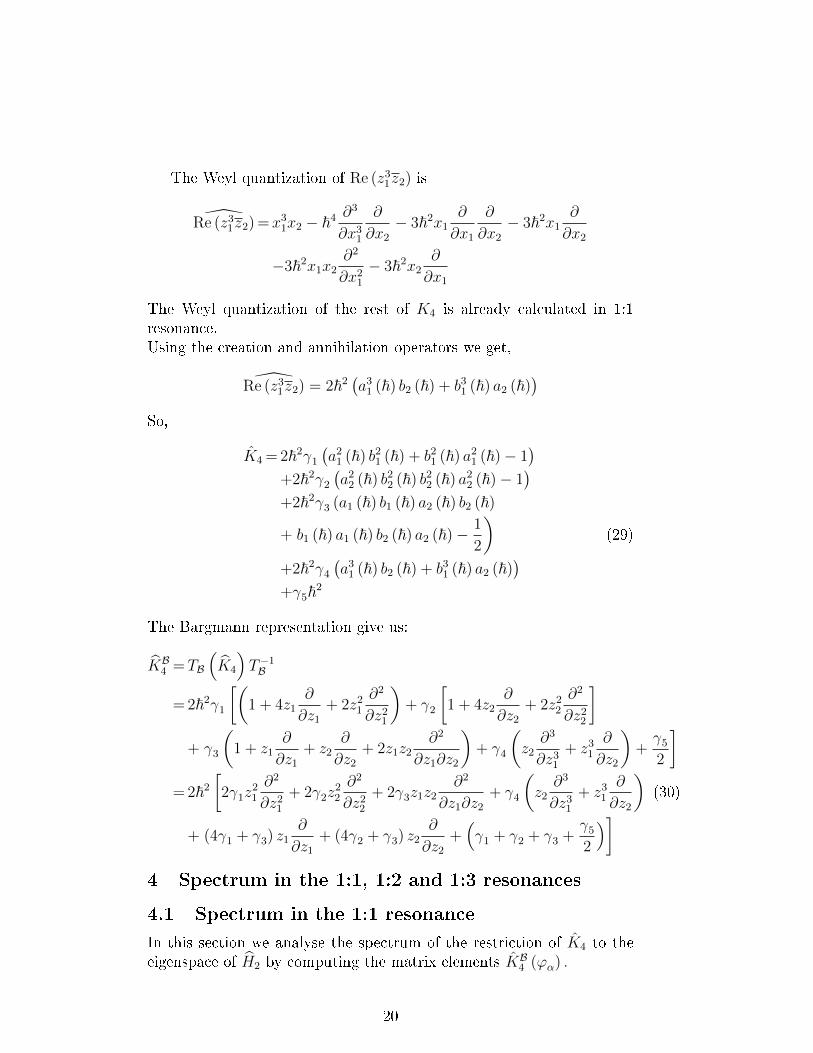
The Weyl quantization of the rest of K4 is already calculated in 1:1resonance.Using the creation and annihilation operators we get,
Re (z31z2) = 2~2
(a3
1 (~) b2 (~) + b31 (~) a2 (~)
)So,
K4 = 2~2γ1
(a2
1 (~) b21 (~) + b2
1 (~) a21 (~)− 1
)+2~2γ2
(a2
2 (~) b22 (~) b2
2 (~) a22 (~)− 1
)+2~2γ3 (a1 (~) b1 (~) a2 (~) b2 (~)
+ b1 (~) a1 (~) b2 (~) a2 (~)− 1
2
)(29)
+2~2γ4
(a3
1 (~) b2 (~) + b31 (~) a2 (~)
)+γ5~2
The Bargmann representation give us:
KB4 =TB
(K4
)T−1B
= 2~2γ1
[(1 + 4z1
∂
∂z1
+ 2z21
∂2
∂z21
)+ γ2
[1 + 4z2
∂
∂z2
+ 2z22
∂2
∂z22
]+ γ3
(1 + z1
∂
∂z1
+ z2∂
∂z2
+ 2z1z2∂2
∂z1∂z2
)+ γ4
(z2∂3
∂z31
+ z31
∂
∂z2
)+γ5
2
]= 2~2
[2γ1z
21
∂2
∂z21
+ 2γ2z22
∂2
∂z22
+ 2γ3z1z2∂2
∂z1∂z2
+ γ4
(z2∂3
∂z31
+ z31
∂
∂z2
)(30)
+ (4γ1 + γ3) z1∂
∂z1
+ (4γ2 + γ3) z2∂
∂z2
+(γ1 + γ2 + γ3 +
γ5
2
)]4 Spectrum in the 1:1, 1:2 and 1:3 resonances
4.1 Spectrum in the 1:1 resonance
In this section we analyse the spectrum of the restriction of K4 to theeigenspace of H2 by computing the matrix elements KB4 (ϕα) .
20

First we have,
∂ϕ(α1,α2)
∂z1
=∂
∂z1
(zα1
1√α1!
zα22√α2!
)= α1
zα1−11√α1!
zα22√α2!
=√α1
zα1−11√
(α1 − 1)!
zα22√α2!
=√α1ϕ(α1−1,α2)
∂2ϕ(α1,α2)
∂z21
=√α1
√α1 − 1ϕ(α1−2,α2)
∂ϕ(α1,α2)
∂z2
=√α2ϕ(α1,α2−1)
∂2ϕ(α1,α2)
∂z22
=√α2
√α2 − 1ϕ(α1,α2−2)
∂2ϕ(α1,α2)
∂z1∂z2
=√α1
√α2ϕ(α1−1,α2−1)
and
z1ϕ(α1,α2) = z1
(zα1
1√α1!
zα22√α2!
)=zα1+1
1√α1!
zα22√α2!
=√α1 + 1
zα1+11√
(α1 + 1)!
zα22√α2!
=√α1 + 1ϕ(α1+1,α2)
z21ϕ(α1,α2) =
√α1 + 2
√α1 + 1ϕ(α1+2,α2)
z2ϕ(α1,α2) =√α2 + 1ϕ(α1,α2+1)
z22ϕ(α1,α2) =
√α2 + 2
√α2 + 1ϕ(α1,α2+2)
z1z2ϕ(α1,α2) =√α1 + 1
√α2 + 1ϕ(α1+1,α2+1)
Thus,
KB4 ϕ(α1,α2) = 2~2(2λ1z21
∂2ϕ(α1,α2)
∂z21
+ 2λ2z22
∂2ϕ(α1,α2)
∂z22
+ 2λ3z1z2
∂2ϕ(α1,α2)
∂z1∂z2
+λ4[z22
∂2ϕ(α1,α2)
∂z21
+ z21
∂2ϕ(α1,α2)
∂z22
] + (4λ1 + λ3) z1
∂ϕ(α1,α2)
∂z1
+ (4λ2 + λ3) z2
∂ϕ(α1,α2)
∂z2
+
(λ1 + λ2 + λ3 +
λ5
2
)ϕ(α1,α2))
= 2~2(2λ1z21
√α1(α1 − 1)ϕ(α1−2,α2) + 2λ2z
22
√α2(α2 − 1)ϕ(α1,α2−2)
+2λ3z1z2
√α1α2ϕ(α1−1,α2−1) + λ4(z2
2
√α1(α1 − 1)ϕ(α1−2,α2)
+z21
√α2(α2 − 1)ϕ(α1,α2−2)) + (4λ1 + λ3) z1
√α1ϕ(α1−1,α2)
+ (4λ2 + λ3) z2
√α2ϕ(α1,α2−1) +
(λ1 + λ2 + λ3 +
λ5
2
)ϕ(α1,α2))
21

= 2~2[2λ1α1 (α1 − 1)ϕ(α1,α2) + 2λ2α2 (α2 − 1)ϕ(α1,α2) + 2λ3α1α2ϕ(α1,α2)
+λ4
(√α1(α1 − 1)(α2 + 1)(α2 + 2)ϕ(α1−2,α2+2)
+√
(α1 + 1)(α1 + 2)α2(α2 − 1)ϕ(α1+2,α2−2)))]
+ (4λ1 + λ3)α1ϕ(α1,α2) + (4λ2 + λ3)α2ϕ(α1,α2) +
(λ1 + λ2 + λ3 +
λ5
2
)ϕ(α1,α2)
= 2~2{λ4
√α1(α1 − 1)(α2 + 1)(α2 + 2)ϕ(α1−2,α2+2)
+ [2λ1α1 (α1 − 1) + 2λ2α2 (α2 − 1) + 2λ3α1α2 + (4λ1 + λ3)α1
+ (4λ2 + λ3)α2 +
(λ1 + λ2 + λ3 +
λ5
2
)]ϕ(α1,α2)
+ λ4
√(α1 + 1)(α1 + 2)α2(α2 − 1)ϕ(α1+2,α2−2)
}We see that the basis HBN is stable by KB4 because,
α1− 2 + (α2 + 2) = α1 +α2 = N and α1 + 2 + (α2 − 2) = α1 +α2 = N
where HBN ={ϕ(N−`,`) ; ` = 0, 1, ..., E
[N2
]}.
One can verify easily that the matrix KB4 in HBN is symetric. Indeed,
KB4 ϕ(α1+2,α2−2) = 4~2[λ4
√(α1 + 2) (α1 + 1) (α2 − 1)α2ϕ(α1,α2) +
(2λ1 (α1 + 2) (α1 + 1) + 2λ2 (α2 − 2) (α2 − 3)
+2λ3 (α1 + 2) (α2 − 2) + (4λ1 + λ3) (α1 + 2)
+ (4λ2 + λ3) (α2 − 2) +
(λ1 + λ2 + λ3 +
λ5
2
))ϕ(α1+2,α2−2)
+λ4
√(α1 + 4) (α1 + 3) (α2 − 2) (α2 − 3)ϕ(α1+4,α2−4)]
One gets,
KB4 ϕ(N−`,`) = 4~2(λ4
√(`+ 1) (`+ 2) (N − `) (N − `− 1)ϕ(N−`−2,`+2)
+(2λ1 (N − `) (N − `− 1) + 2λ2` (`− 1) + λ3 (N − `) ` (31)
+ (4λ1 + λ3) (N − `) + (4λ2 + λ3) `+
(λ1 + λ2 + λ3 +
λ5
2
))ϕ(N−`,`)
+ λ4
√` (`− 1) (N − `+ 1) (N − `+ 2)ϕ(N−`+2,`−2)
)Thus,
22
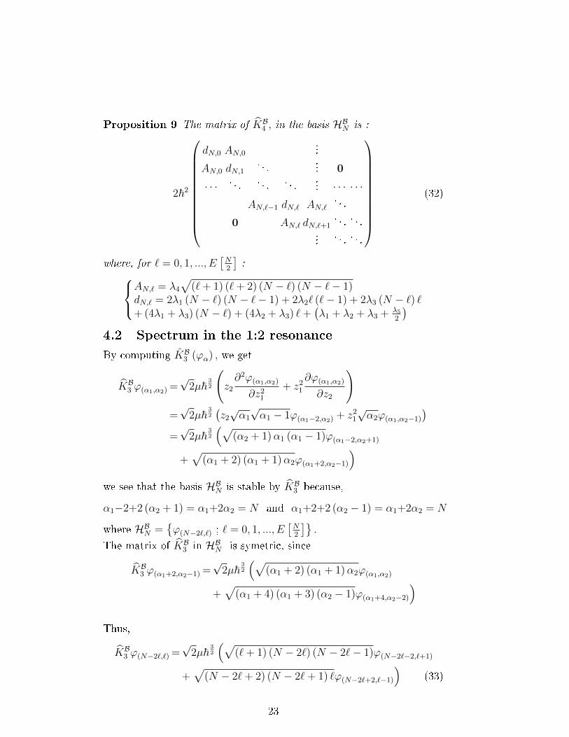
Proposition 9 The matrix of KB4 , in the basis HBN is :
2~2
dN,0 AN,0...
AN,0 dN,1. . .
... 0
· · · . . . . . . . . .... · · · · · ·
AN,`−1 dN,` AN,`. . .
0 AN,` dN,`+1. . . . . .
.... . . . . .
(32)
where, for ` = 0, 1, ..., E[N2
]:AN,` = λ4
√(`+ 1) (`+ 2) (N − `) (N − `− 1)
dN,` = 2λ1 (N − `) (N − `− 1) + 2λ2` (`− 1) + 2λ3 (N − `) `+ (4λ1 + λ3) (N − `) + (4λ2 + λ3) `+
(λ1 + λ2 + λ3 + λ5
2
)4.2 Spectrum in the 1:2 resonance
By computing KB3 (ϕα) , we get
KB3 ϕ(α1,α2) =√
2µ~32
(z2
∂2ϕ(α1,α2)
∂z21
+ z21
∂ϕ(α1,α2)
∂z2
)=√
2µ~32
(z2
√α1
√α1 − 1ϕ(α1−2,α2) + z2
1
√α2ϕ(α1,α2−1)
)=√
2µ~32
(√(α2 + 1)α1 (α1 − 1)ϕ(α1−2,α2+1)
+√
(α1 + 2) (α1 + 1)α2ϕ(α1+2,α2−1)
)we see that the basis HBN is stable by KB3 because,
α1−2+2 (α2 + 1) = α1+2α2 = N and α1+2+2 (α2 − 1) = α1+2α2 = N
where HBN ={ϕ(N−2`,`) ; ` = 0, 1, ..., E
[N2
]}.
The matrix of KB3 in HBN is symetric, since
KB3 ϕ(α1+2,α2−1) =√
2µ~32
(√(α1 + 2) (α1 + 1)α2ϕ(α1,α2)
+√
(α1 + 4) (α1 + 3) (α2 − 1)ϕ(α1+4,α2−2)
)Thus,
KB3 ϕ(N−2`,`) =√
2µ~32
(√(`+ 1) (N − 2`) (N − 2`− 1)ϕ(N−2`−2,`+1)
+√
(N − 2`+ 2) (N − 2`+ 1) `ϕ(N−2`+2,`−1)
)(33)
23

Proposition 10 The matrix of KB3 in the basis HBN is:
√2µ~
32
0 m0...
m0 0. . .
... 0
· · · . . . 0 m` · · · · · ·m` 0
. . .
0. . . 0
. . ..... . . 0
(34)
where for ` = 0, 1, ..., E[N2
]:
m` =√
(`+ 1) (N − 2`) (N − 2`− 1)
In the case of Fermi resonance, the half integer powers of ~ arepresent, the coe�cient of ~3/2 is then the average along the �ow of H2
of the term of order 3 in the Taylor expansion of the symbol.
4.3 Spectrum in the 1:3 resonance
We have,
∂3ϕ(α1,α2)
∂z31
=√α1
√α1 − 1
√α1 − 2ϕ(α1−3,α2)
z31ϕ(α1,α2) =
√α1 + 3
√α1 + 2
√α1 + 1ϕ(α1+3,α2)
then,
z31
∂ϕ(α1,α2)
∂z2
+ z2
∂3ϕ(α1,α2)
∂z31
=√
(α1 + 3)(α1 + 2)(α1 + 1)α2ϕ(α1+3,α2−1)
+√α1(α1 − 1)(α1 − 2)(α2 + 1)ϕ(α1−3,α2+1)
Therefore,
KB4 ϕ(α1,α2) = 2~2(γ4
√α1 (α1 − 1) (α1 − 2) (α2 + 1)ϕ(α1−3,α2+1)
+(2γ1α1(α1 − 1) + 2γ2α2(α2 − 1) + 2γ3α1α2 + (4γ1 + γ3)α1
+ (4γ2 + γ3)α2 +(γ1 + γ2 + γ3 +
γ5
2
))ϕ(α1,α2)
+γ4
√(α1 + 3) (α1 + 2) (α1 + 1)α2ϕ(α1+3,α2−1)
)The basisHBN =
{ϕ(N−3`,`) ; ` = 0, 1, ..., E
[N2
]}is stable by KB4 because,
α1+3+3 (α2 − 1) = α1+3α2 = N and α1−3+3 (α2 + 1) = α1+3α2 = N
24

and the matrix of KB4 in HBN is symetric since
KB4 ϕ(α1+3,α2−1) = 2~2[γ4
√(α1 + 3) (α1 + 2) (α1 + 1)α2ϕ(α1,α2)
+ (2γ1 (α1 + 3) (α1 + 2) + 2γ2 (α2 − 1) (α2 − 2) + 2γ3 (α1 + 3) (α2 − 1)
+ (4γ1 + γ3) (α1 + 3) + (4γ2 + γ3) (α2 − 1)
+(γ1 + γ2 + γ3 +
γ5
2
)]ϕ(α1+3,α2−1)
+γ4
√(α1 + 6) (α1 + 5) (α1 + 4) (α2 − 1)ϕ(α1+6,α2−2)
]So one gets,
KB4 ϕ(N−3`,`) = 2~2(γ4
√(`+ 1) (N − 3`) (N − 3`− 1) (N − 3`− 2)ϕ(N−3`−3,`+1)
+[2γ1 (N − 3`) (N − 3`− 1) + 2γ2` (`− 1) + 2γ3` (N − 3`) (35)
+ (4γ1 + γ3) (N − 3`) + (4γ2 + γ3) `+(γ1 + γ2 + γ3 +
γ5
2
)]ϕ(N−3`,`)
+ γ4
√` (N − 3`+ 1) (N − 3`+ 2) (N − 3`+ 3)ϕ(N−3`+3,`−1)
)and therefore,
Proposition 11 The matrix of KB4 in the basis HBN is :
2~2
d′N,0 BN,0...
BN,0 d′N,1
. . . . . .... 0
· · · . . . . . .BN,`−1 · · · · · ·. . . d′N,` BN,`
. . .
0 BN,` d′N,`+1
. . . . . ....
. . . . . .
(36)
where for ` = 0, 1, ..., E[N2
]:
BN,` = γ4
√(`+ 1) (N − 3`) (N − 3`− 1) (N − 3`− 2)
d′N,` = (2γ1 (N − 3`)2 + 2γ2`2 + 2γ3` (N − 3`)
+ (3γ1 + γ3) (N − 3`) + (3γ2 + γ3) `+(γ1 + γ2 + γ3 + γ5
2
))
5 An e�ective Quantum BGNF program
We have implemented the Quantum Birkho�-Gustavson normal formin the computer language ocaml(2), which is a fast and very expressivefunctional language, particularly well adapted to mathematical construc-tions.
(2)http://caml.inria.fr/index.en.html
25

5.1 Overview of the code
The code consists of three modules : Math, Weyl and Birkhoff. TheMath module is a functorial interface that de�nes the axioms of general(non-commutative) associative algebras over an abelian �eld. This per-mits the use of the same code for di�erent coe�cient rings: real numbers,complex numbers, rationals, or even formal series. For instance, we maydeclare that we use complex coe�cients using the simple line :
open Math.ComplexNumbers;;
The Weyl module implements the Weyl algebra for formal series E �de�ned in Section 2, endowed with the non-commutative Moyal product.Internally, series are stored in hash tables, and the module provides a wayto convert them to/from a text representation. The number of variablesis arbitrary, it need not be speci�ed. For instance the 1 : 2-oscillator
h2 =1
2(x2
1 + ξ21) + (x2
2 + ξ22)
will be printed as follows:
Weyl.print_poly h2;;
1 h^0 x^() ξ^(0,2)1 h^0 x^(0,2) ξ^()0.5 h^0 x^() ξ^(2)0.5 h^0 x^(2) ξ^()
For convenience, we also wrote a Maple module that can use copy-pasted text directly to/from Maple notation :
Maple.of_poly h2;;
- : string = "0.5*x[1]^2+0.5*xi[1]^2+1*x[2]^2+1*xi[2]^2"
As a simple example, the code below computes the Moyal bracketof x3 and ξ3 � which is the Weyl symbol of the operator bracketi~ [x3, (~
i∂∂x
)3].
let x3 = Maple.to_poly "x[1]^3" in
let xi3 = Maple.to_poly "xi[1]^3" inlet c = Weyl.crochet x3 xi3 in
Maple.of_poly c;;
- : string = "1.5*h^2+-9*x[1]^2*xi[1]^2"
Thus we �nd ih[x3, ξ3]W = 3
2~2 − 9x2ξ2.
26

The Birkhoff module is the core of the normal form algorithm. Itimplements the proof of Theorem 1 that appears in [5]. It involves aninduction where each step consists in solving a cohomological equation.Only Moyal brackets, additions, and multiplication by scalar are used.Here is the code for the induction step :
let birkhoff_step order freq k r =
let n = ordre r inlet (rn, _) = get_homog r n in
let (kn, an) = split freq rn in
let newh = exp_ad an (add k r) order
and k' = add k kn
in let r' = add newh (coeff_mult C.mone k') inproj_order ~check:true r' (n+1);
(k', r')
If h=k+r, where h is the initial quantum Hamiltonian (or Weyl sym-bol), k is the normalisation at order n-1 and r is the remainder (of ordern, then the function birkhoff_step computes the next-order normal-ization : h=k'+r', where r' is of order n+1.
For simplicity, we have assumed in this code that the quadratic hamil-tonian is of the formH2 = ν1x
′1ξ′1+· · ·+νnx′nξ′n : this amounts to writing
H2 in terms of creation and annihilation operators as in (6). In orderto deal with harmonic oscillators in real variables (xj, ξj) as in (2), weneed to use the change of variables x′j = 1√
2(xj + iξj), ξ
′j = 1√
2(xj − iξj).
We have implemented this change of variables in the code.
5.2 Numerical results for the 1 : 3 resonance
We may de�ne H2 using Maple notation as follows :
let h2 = Maple.to_poly "0.5*x[1]^2+0.5*xi[1]^2+1.5*x[2]^2+1.5*xi[2]^2";;
Then we convert it to complex coordinates :
let h2z = coordz h2;;Maple.of_poly h2z;;
- : string = "1*x[1]^1*xi[1]^1+3*x[2]^1*xi[2]^1"
It has now the required formH2 = x′1ξ′1+3x′2ξ
′2. We add now a simple
perturbation W = (x2)3, which we convert to complex coordinates :
let w = Maple.to_poly "x[2]^3";;
let wz = coordz w;;Maple.of_poly vz;;
27

- : string =
"1.06066*x[2]^1*xi[2]^2+0.353553*x[2]^3+
1.06066*x[2]^2*xi[2]^1+0.353553*xi[2]^3"
Thus we have, in complex coordinates (x′j, ξ′j) :
W =17
16x′2ξ
′2
2+
6
17x′2
3+
17
16x′2
2ξ′2 +
6
17ξ′2
3.
and �nally we may consider the hamiltonian H = H2 +W :
let hz = Weyl.add h2z vz;;
Now we de�ne the frequency vector [1; 3], and we may apply theBirkho� procedure at order 4 :
let freq = [| one; of_int 3 |];;let kz = birkhoff freq hz 4;;
We have obtained the normalized Hamiltonian kz. We convert itback to real coordinates (xj, ξj) and print it :
let k = coordx kz;;Maple.of_poly k;;
- : string =
"0.5*x[1]^2+0.5*xi[1]^2+0.166667*h^2+-0.625*x[2]^2*xi[2]^2+-0.3125*x[2]^4+
-0.3125*xi[2]^4+1.5*x[2]^2+1.5*xi[2]^2"
Reordering terms, we get
K =1
2x2
1+1
2ξ2
1+3
2x2
2+3
2ξ2
2+1
6~2−5
8x2
2ξ22−
5
16x4
2−5
16ξ4
2+O6 = H2+K4+O6
where K4 = 16~2 − 5
8x2
2ξ22 − 5
16x4
2 − 516ξ4
2 = 16~2 − 5
16(x2
2 + ξ22)2.
It remains to compare to the theoretical results of section 3.5 (The-orem 8), which predicts:
K4 = γ1 |z1|4 + γ2 |z2|4 + γ3 |z1|2 |z2|2 + γ4 Re(z3
1z2
)+ γ5~2
Using that W (x1, x2) = x32, we see from the formulas in Theorem 8
28

that only the coe�cients γ2 and γ5 don't vanish; we obtain:
K4 = γ2 |z2|4 + γ5~2
=−1
2
(1
3!2√
2
)2
20
(∂3W (0)
∂x32
)21
4
(x4
2 + ξ42 + 2x2
2ξ22
)+
1
216
(∂3W (0)
∂x32
)2
~2
=−1
2
(1
3!2√
2
)2
20.36.1
4
(x4
2 + ξ42 + 2x2
2ξ22
)+
1
216.36.~2
=− 5
16
(x4
2 + ξ42 + 2x2
2ξ22
)+
1
6~2
hence,
H2 +K4 =1
2x2
1 +1
2ξ2
1 +3
2x2
2 +3
2ξ2
2 −5
16x4
2 −5
16ξ4
2 −5
8x2
2ξ22 +
1
6~2,
which con�rms the computer output.Of course, we can ask the program to give the normalization at any
given order. For instance here is what we get at order 8 :
K =1
2ξ2
1 +3
2ξ2
2 +1
2x2
1 +3
2x2
2
− 5
16ξ4
2 +1
6~2 − 5
8x2
2ξ22 −
5
16x4
2
− 235
1152ξ6
2 +395
576~2ξ2
2 −235
384x2
2ξ42 −
235
384x4
2ξ22 −
235
1152x6
2 +395
576~2x2
2
− 38585
165888ξ8
2 +100205
41472~2ξ4
2 −128
243~4 − 38585
41472x2
2ξ62 −
38585
27648x4
2ξ42 −
38585
41472x6
2ξ22
− 38585
165888x8
2 +100205
20736~2x2
2ξ22 +
100205
41472~2x4
2 +O10
References
[1] M. K. Ali, The quantum normal form and its equivalents. J. Math.Phys, 26 (10) (1985), 2565-2572.
[2] D. Bambusi, Semiclassical normal forms. In: Multiscale Methodesin Quantum Mecanics. Trends in Math. Birkhäuser, Boston (2004),23-39.
[3] V. Bargmann, On a Hilbert Space of Analytic Functions and an As-sociated Integral Transform, Part I, Comm. Pure and Appl. Math.(14) (1967), 187-214.
[4] G. D. Birkho�, Dynamical systems. AMS, (1927).[5] L. Charles and S. Vu Ngoc, Spectral asymptotics via the semiclas-
sical Birkho� normal form. Duke Math. J. Vol. 143, N◦3 (2008),463-511.
29

[6] B. Eckhardt, Birkho�-Gustavson normal form in classical and quan-tum mechanics. J. Phys. A, 19 (1986), 2961-2972.
[7] K. Ghomari, B. Messirdi, Quantum Birkho�-Gustavson NormalForm in some completely resonant cases. J. Math. Anal. App 378(2011) 306-313.
[8] F. G. Gustavson, On constructing formal integrals of a Hamiltoniansystem near an equilibrium point. Astron. J, 83(2) (1966), 287-352.
[9] M. Joyeux, Gustavson's procedure and the dynamics of highly ex-cited vibrational states. J. Chem. Phys, 109 (1998), 337-408.
[10] D. Robert and M. Joyeux, Canonical perturbation theory versusBorn-Oppenheimer-type separation of motions: the vibrational dy-namics of C3. J. Chem. Phys, 119 (2003), 8761-8762.
[11] J. Sjostrand, Semi excited states in nondegenerate potential wells.Asymptotic Anal, (6) (1992), 29-49.
[12] R. T. Swimm and J. B. Delos, Semiclassical calculations of vibra-tional energy levels for nonseparable systems using the Birkho�-Gustavson normal form. J . Chem. Phys, 71(4) (1979), 1706-1717.
30