Asteristique 226, pp. 235-320.

Bloch’s higher Chow groups revisited

Marc Levine

IntroductionBloch defined his higher Chow groups CHq(−, p) in [B], with the object of defining an integral cohomologytheory which rationally gives the weight–graded pieces Kp(−)(q) of K-theory. For a variety X, the higherChow group CHq(X, p) is defined as the pth homology of the complex Zq(X, ∗), which in turn is built outof the codimension q cycles on X × Ap for varying p, using the cosimplicial structure on the collection ofvarieties X ×Ap | p = 0, 1, . . .. In order to relate CHq(X, p) with Kp(X), Bloch used Gillet’s constructionof Chern classes with values in a Bloch-Ogus twisted duality theory [G]; this requires, among other things,that the complexes Zq(X, ∗) satisfy a Mayer-Vietoris property for the Zariski topology, and that they satisfya contravariant functoriality. Bloch attempted to prove the Mayer-Vietoris property by proving a localizationtheorem, identifying the cone of the restriction map

Zq(X, ∗) → Zq(U, ∗),

for U → X a Zariski open subset of X, with the complex Zq(X \ U, ∗)[1], up to quasi-isomorphism. Thereis a gap in Bloch’s proof, which left open the localization property and the Mayer-Vietoris property for thecomplexes Zq(X, ∗); essentially the same problem leaves a gap in the proof of contravariant functoriality.Recently, Bloch [B3] has provided a new argument which fills the gap in the proof of localization; this,together with a new argument for contravariant functoriality, should allow Bloch’s original program forrelating CHq(X, p) with Kp(X) to go through without further problem.

As part of the argument in [B], Bloch defined a map

(1) CHq(X, p)⊗Q→ Kp(X)(q)

for X smooth and quasi-projective over a field, relying on a λ-ring structure on relative K-theory withsupports. It turns out that this approach can be followed and extended to show that the map (1) is anisomorphism, without relying on Chern classes (Theorem 3.1). An important new ingredient in this line ofargument is the computation of certain relative K0-groups in terms of the K0 of an associated iterated double(see Theorem 1.10 and Corollary 1.11). A bit more work then enables us to prove the Mayer-Vietoris property(Theorem 3.3), a weak version of localization (Theorem 3.4) and contravariant functoriality (Corollary 4.9)for the rational complexes Zq(X, ∗)⊗Q. We also construct a product for the rational complexes Zq(X, ∗)⊗Qand prove the projective bundle formula (Corollary 5.4). The arguments used in [B] then give rational Chernclasse

cq,p : K2q−p(X) → CHq(X, 2q − p)⊗Q,

satisfying the standard properties.It turns out that it is somewhat more convenient to work with a modified version of Zq(X, ∗), using

a cubical structure rather than a simplicial structure. We show that the cubical complexes Zq(X, ∗)c areintegrally quasi-isomorphic to the simplicial version Zq(X, ∗) (Theorem 4.7), and have a natural externalproduct in the derived category (see §5, especially Theorem 5.2). We also consider the “alternating” com-plexes Nq(k) defined by Bloch [B2], and used to construct a candidate for a motivic Lie algebra. We showthat there is a natural quasi-isomorphism

Zq(Spec(k), ∗)c ⊗Q→ Nq(k)

1

(Theorem 4.11). The product structures are not quite compatible via this quasi-isomorphism; it is necessaryto reverse the order of the product in one of the complexes to get a product-compatible quasi-isomorphism(Corollary 5.5).

The paper is organized as follows: We begin in §1 by proving some extensions of the results of Vorston Kn-regularity, which we use to prove a basic result on the K0-regularity of certain iterated doubles. Wealso recall some basic facts about relative K-theory, and use the K0-regularity results to compute certainrelative K0 groups in terms of the usual K0 of an iterated double. In §2 we use, following Bloch, the λ-operations on relative K-theory with supports to give a cycle-theoretic interpretation of certain relative K0

groups, analogous to the classical Grothendieck-Riemann-Roch theorem relating the rational Chow ring tothe rational K0 for a smooth variety (see Theorem 2.7). In §3, we use this to show that Bloch’s map

CH1(X, p)⊗Q→ Kp(X)(q)

is an isomorphism for X smooth and quasi-projective. In §4, we relate the cubical complexes with Bloch’ssimplicial version, and also with his alternating version. In §5 we define products and prove the projectivebundle formula for the rational complexes.

As a matter of notation, a scheme will alsways mean a separated, Noetherian scheme. For an abeliangroup A, we denote A⊗Q by AQ; for a homological complex C∗, we deonte the cycles in degree p by Zp(C∗),the boundaries by Bp(C∗) and the homology by Hp(C∗).

We would like to thank Spencer Bloch and Stephen Lichtenbaum for their encouragement and sugges-tions, and thank as well the organizers of the Strasbourg K-theory conference for assembling this volume.We would also like to thank Dan Grayson for his comments on an earlier version of this paper, and especiallythank Chuck Weibel for pointing out the need for the K0-regularity results in §1, and suggesting the use ofhis homotopy K-theory functor KH.

§1. NK and relative K0

In this section, we give a description of relative K0, K0(X;Y1, . . . , Yn), in terms of the K0 of the so-callediterated double D(X;Y1, . . . , Yn). We begin by extending some of Vorst’s results on NKp of rings to schemesover a ring.

Fix a commutative ring A, and let AlgA denote the category of commutative A-algebras, Ab thecategory of abelian groups. For a ring R, let pR:R[T ] → R be the R-algebra homomorphism pR(T ) = 0. Fora functor F :AlgA → Ab, let NF :AlgA → Ab be the functor

NF (R) = ker[F (pR):F (R[T ]) → F (R)].

Define the associated functors NqF for q > 1 inductively by

NqF = N(Nq−1F ).

We set N0F = F .For R ∈ AlgA and r ∈ R, the R-algebra map

φr:R[T ] → R[T ]φr(T ) = rT

gives rise to the endomorphism NF (φr):NF (R) → NF (R), thus NF (R) becomes a Z[T ]-module with Tacting via φr. Let NF (R)[r] denote the localization Z[T, T−1] ⊗Z[T ] NF (R). If r is a unit, then the mapNF (R) → NF (R)[r] is an isomorphism; letting Rr denote the localization of R with respect to the powersof r, the natural map

NF (R) → NF (Rr)

2

factors canonically through N(R)[r]:

NF (R) → NF (R)[r]

NF (Rr)

For elements r1, . . . , rn of R, form the “augmented Cech complex”

(1.1)

0 →NF (R) ε→⊕

1≤i≤nNF (Rri

) → . . .

→⊕

1≤i0<i1<...<ip≤nNF (Rri0 ,ri1 ,...,rip

) → . . .→ NF (Rr1,...,rn)to0.

where the map

⊕1≤i0<i1<...<ip≤n

NF (Rri0 ,ri1 ,...,rip) →

⊕1≤i0<i1<...<ip+1≤n

NF (Rri0 ,ri1 ,...,rip+1)

is given as the direct sum over indices (1 ≤ i0 < i1 < . . . < ip+1 ≤ n) of the alternating sums:

p+1∑j=0

(−1)jδj :⊕p+1j=0NF (R

ri0 ,...,rij,...,rip+1

) → NF (Rri0 ,...,rip+1),

and where

δj :NF (Rri0 ,...,rij

,...,rip+1) → NF (Rri0 ,...,rip+1

)

is the canonical map. The map ε is the direct sum of the canonical maps

NF (R) → NF (Rrj ).

Lemma 1.1. Suppose R is a commutative A-algebra, r1, . . . , rn elements of R which generate the unit ideal.Suppose further that the map

NF (R[T ]ri0 ,...,rij

,...,rip)[rij

] → NF (R[T ]ri0 ,...,rip)

is an isomorphism, for each set of indicies 1 ≤ i0 < . . . < ip ≤ n. Then the complex (1.1) is exact. Inparticular, the map

ε:NF (R) → ⊕nj=1NF (Rrj )

is injective.

Proof. This is proved in ([V], Theorem 1.2); there the functor F is a functor from AlgZ to Ab, but, as theproof uses only the restriction of F to the category AlgR, the argument works as well in the case of a functorF :AlgA → Ab.

3

Let X be a scheme. We let PZ denote the category of locally free sheaves of finite rank on X, and letK(X) denote the space ΩBQPZ ; the pth the K-group Kp(X), p ≥ 0, is thus defined as the homotopy groupπp(K(X)). Letting A1

X denote the affine line over X, and GmX the open subscheme A1X\0X , we have the

“fundamental exact sequence” for p ≥ 0

(1.2) 0 → Kp+1(X) → Kp+1(A1X)⊕Kp+1(A1

X) → Kp+1(GmX) → Kp(X) → 0

where the maps are those arising from a spectral sequence computing the K-groups of P1X via the standard

cover

P1X = A1

X ∪ A1X .

This allows the inductive definition of the K-groups Kp(X) for p < 0 by forcing the exactness of

Kp+1(A1X)⊕Kp+1(A1

X) → Kp+1(GmX) → Kp(X) → 0

for all p; it then follows (see [*]) that the sequence (1.2) is exact for all p ∈ Z.Let i0:X → A1

X be the inclusion as the zero section. Recall the inductive definition of the groupsNqKp(X) as

NqKp(X) =Kp(X) for q=0,ker[i∗0:N

q−1Kp(A1X) → Nq−1Kp(X)] for q > 0.

We recall that a scheme X is Kp-regular if NqKp(X) = 0 for each q > 0.Let U = Uα be a Zariski open cover of X. Then there is a spectral sequence (see Thomason [T], *)

(1.3) Ep,q1 = ⊕(α0,...,αq)NtK−p(Uα0 ∩ . . . ∩ Uαq ) ⇒ N tK−p−q(X).

The E2-term is the Cech cohomology with coefficients in the presheaf NqK−p: Hq

Cech(U,N tK−p); the se-

quence is strongly convergent for finite covers.For an A-scheme X, and element f ∈ A, we let Xf denote the open subscheme defined by the non-

vanishing of f . Let FX :AlgA → Ab be the functor

FX(R) = Kp(X ⊗A R);

in particular, we have NqF (R) = NqKp(X ⊗A R). For f ∈ A, we use the notation NqKp(X)[f ] forNqFX(A)[f ].

Lemma 1.2. Let A be a commutative ring, f ∈ A and X an A-scheme. Suppose we have a covering of Xby affine open subsets Uα = Spec(Aα) such that, for each α, either f is a non-zero divisor in Aα, or f iscontained in some minimal prime ideal of Aα. Then the natural map

NqKp(X)[f ] → NqKp(Xf )

is an isomorphism.

Proof. Let B be a commutative ring and suppose g ∈ B is either a non-zero divisor in B, or is contained insome minimal prime ideal of B. Then Vorst ([V], Lemma 1.4) has shown that the natural map

NqKp(B)[g] → NqKp(Bg)

is an isomorphism (Vorst only proves this for p ≥ 0, but the general result follows from this and thefundamental exact sequence (1.2)). The general result follows from this and the spectral sequence (1.3).

4

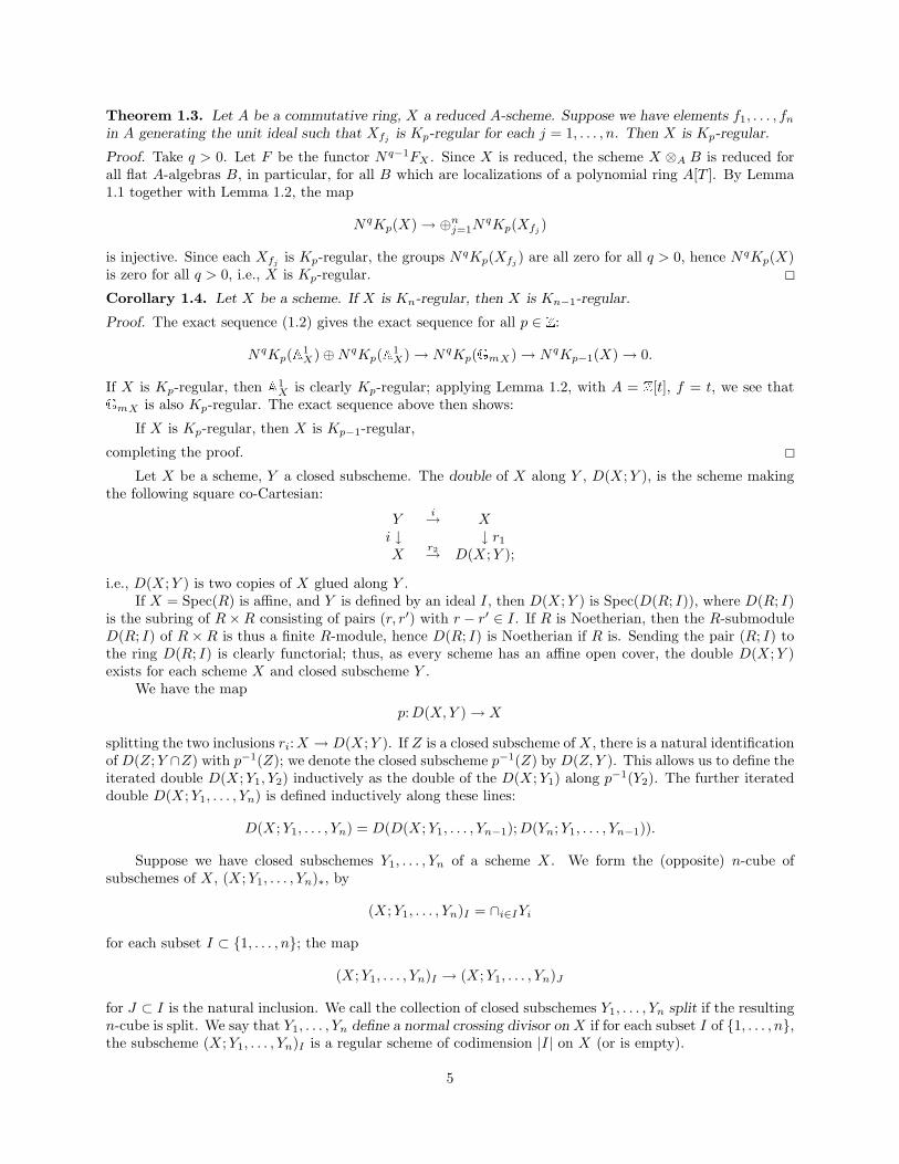
Theorem 1.3. Let A be a commutative ring, X a reduced A-scheme. Suppose we have elements f1, . . . , fnin A generating the unit ideal such that Xfj is Kp-regular for each j = 1, . . . , n. Then X is Kp-regular.

Proof. Take q > 0. Let F be the functor Nq−1FX . Since X is reduced, the scheme X ⊗A B is reduced forall flat A-algebras B, in particular, for all B which are localizations of a polynomial ring A[T ]. By Lemma1.1 together with Lemma 1.2, the map

NqKp(X) → ⊕nj=1NqKp(Xfj )

is injective. Since each Xfj is Kp-regular, the groups NqKp(Xfj ) are all zero for all q > 0, hence NqKp(X)is zero for all q > 0, i.e., X is Kp-regular.

Corollary 1.4. Let X be a scheme. If X is Kn-regular, then X is Kn−1-regular.

Proof. The exact sequence (1.2) gives the exact sequence for all p ∈ Z:

NqKp(A1X)⊕NqKp(A1

X) → NqKp(GmX) → NqKp−1(X) → 0.

If X is Kp-regular, then A1X is clearly Kp-regular; applying Lemma 1.2, with A = Z[t], f = t, we see that

GmX is also Kp-regular. The exact sequence above then shows:

If X is Kp-regular, then X is Kp−1-regular,

completing the proof.

Let X be a scheme, Y a closed subscheme. The double of X along Y , D(X;Y ), is the scheme makingthe following square co-Cartesian:

Yi→ X

i ↓ ↓ r1X

r2→ D(X;Y );

i.e., D(X;Y ) is two copies of X glued along Y .If X = Spec(R) is affine, and Y is defined by an ideal I, then D(X;Y ) is Spec(D(R; I)), where D(R; I)

is the subring of R×R consisting of pairs (r, r′) with r − r′ ∈ I. If R is Noetherian, then the R-submoduleD(R; I) of R × R is thus a finite R-module, hence D(R; I) is Noetherian if R is. Sending the pair (R; I) tothe ring D(R; I) is clearly functorial; thus, as every scheme has an affine open cover, the double D(X;Y )exists for each scheme X and closed subscheme Y .

We have the map

p:D(X,Y ) → X

splitting the two inclusions ri:X → D(X;Y ). If Z is a closed subscheme of X, there is a natural identificationof D(Z;Y ∩Z) with p−1(Z); we denote the closed subscheme p−1(Z) by D(Z, Y ). This allows us to define theiterated double D(X;Y1, Y2) inductively as the double of the D(X;Y1) along p−1(Y2). The further iterateddouble D(X;Y1, . . . , Yn) is defined inductively along these lines:

D(X;Y1, . . . , Yn) = D(D(X;Y1, . . . , Yn−1);D(Yn;Y1, . . . , Yn−1)).

Suppose we have closed subschemes Y1, . . . , Yn of a scheme X. We form the (opposite) n-cube ofsubschemes of X, (X;Y1, . . . , Yn)∗, by

(X;Y1, . . . , Yn)I = ∩i∈IYi

for each subset I ⊂ 1, . . . , n; the map

(X;Y1, . . . , Yn)I → (X;Y1, . . . , Yn)J

for J ⊂ I is the natural inclusion. We call the collection of closed subschemes Y1, . . . , Yn split if the resultingn-cube is split. We say that Y1, . . . , Yn define a normal crossing divisor on X if for each subset I of 1, . . . , n,the subscheme (X;Y1, . . . , Yn)I is a regular scheme of codimension |I| on X (or is empty).

5

Lemma 1.5. Let X be a scheme, Y a closed subscheme. Suppose that the inclusion i:Y → X is split.Then the sequence

0 → K0(D(X;Y ))(r∗1 ,r

∗2 )→ K0(X)⊕K0(X)i

∗⊕−i∗→ K0(Y ) → 0

is exact.

Proof. For a scheme Z, let IsoPZ the set of isomorphism classes in PZ ; we let [E] denote the isomorphismclass of a locally free sheaf. The category PD(X;Y ) is equivalent to the category of triples (E,E′, φ), whereE and E′ are locally free sheaves on X, and φ: i∗E → i∗E′ is an isomorphism. Since the inclusion i is split,each automorphism ρ of i∗E lifts to an automorphism ρ of E; thus the isomorphism class of (E,E′, φ) isindependent of the choice of isomorphism φ. Thus, IsoPD(X;Y ) is the set of pairs ([E], [E′]) of isomorphismclasses of locally free sheaves on X, such that i∗[E] = i∗[E′]. Using the splitting of i again, this implies thatthe sequence

Z[IsoPD(X;Y )] → Z[IsoPX ]⊕ Z[IsoPX ] → Z[IsoPY ] → 0

is exact, and the kernel of the first map is generated by elements of the form

(1.4) ([E], [E′])− ([E], [E′′]) + ([F ], [E′′])− ([F ], [E′]).

For a scheme Z, let RZ denote the kernel of the surjection

Z[IsoPZ ] → K0(Z);

i.e., RZ is the subgroup of Z[IsoPZ ] generated by expressions of the form [E]− [E′]− [E′′], where 0 → E′ →E → E′′ → 0 is exact. Since i is split, the sequence

RD(X;Y ) → RX ⊕RX → RY → 0

is exact. On the other hand, for elements ([E], [E′]), ([E], [E′′]),([F ], [E′′]), ([F ], [E′]) in IsoPD(X;Y we havethe relations in K0(D(X;Y )):

([E], [E′]) + ([F ], [E′′]) = ([E ⊕ F ], [E′ ⊕ E′′])= ([E ⊕ F ], [E′′ ⊕ E′])= ([E], [E′′]) + ([F ], [E′]).

Thus, elements of the form (1.4) are contained in RD(X;Y ); a diagram chase finishes the proof.

Theorem 1.6. Let X be a reduced A-scheme, A a reduced commutative ring, and let Y1, . . . , Yn be sub-schemes of X, defining a normal crossing divisor on X. Suppose that there are elements f1, . . . , fk of A suchthat Y1 ∩Xfj

, . . . , Yn ∩Xfjis a split collection of closed subschemes of Xfj

for each j = 1, . . . , k. Then theiterated double D(X;Y1, . . . , Yn) is Kp-regular for all p ≤ 0.

Proof. By Corollary 1.4, we need only consider the case p = 0. If we replace X and Y1, . . . , Yn with AqX andAqY1, . . . ,AqYn

, the hypotheses of the theorem remain valid; thus, we need only show that

N1K0(D(X;Y1, . . . , Yn)) = 0.

We have the natural map

D(X;Y1, . . . , Yn) → X;

6

which identifies the iterated double D(Xf ;Y1 ∩ Xf , . . . , Yn ∩ Xf ) with D(X;Y1, . . . , Yn)f for each f ∈ A.By Theorem 1.3, and our hypotheses, we may assume that the collection of subschemes Y1, . . . , Yn is split.The split, normal crossing hypotheses pass to the collection of closed subschemes Y1 ∩ Yn, . . . , Yn−1 ∩ Yn; byinduction we may assume that D(X;Y1, . . . , Yn−1) and D(Yn;Y1 ∩ Yn, . . . , Yn−1 ∩ Yn) are K0-regular. Ourhypothesis that the collection of subschemes Y1, . . . , Yn is split implies that the natural inclusion

D(Yn;Y1 ∩ Yn, . . . , Yn−1 ∩ Yn) → D(X;Y1, . . . , Yn−1)

is split.The iterated double D(X;Y1, . . . , Yn) is the same as the double of D(X;Y1, . . . , Yn−1) along the sub-

scheme D(Yn;Y1 ∩ Yn, . . . , Yn−1 ∩ Yn); thus we have the commutative diagram

0 0↓ ↓

K0(D(X;Y1, . . . , Yn)) → K0(D(A1X ;A1

Y1, . . . ,A1

Yn))

↓ ↓K0(D(X;Y1, . . . , Yn−1)) K0(D(A1

X ;A1Y1, . . . ,A1

Yn−1))

⊕ → ⊕K0(D(X;Y1, . . . , Yn−1)) K0(D(A1

X ;A1Y1, . . . ,A1

Yn−1))

↓ ↓K0(D(Yn;Y1 ∩ Yn, . . . , Yn−1 ∩ Yn)) → K0(D(A1

Yn;A1Y1∩Yn

, . . . ,A1Yn−1∩Yn

))↓ ↓0 0

By Lemma 1.3, the columns above are exact; since D(X;Y1, . . . , Yn−1) and D(Yn;Y1 ∩ Yn, . . . , Yn−1 ∩ Yn)are K0-regular, and we have natural isomorphisms

D(A1X ;A1

Y1, . . . ,A1

Yn−1) → A1

D(X;Y1,...,Yn−1)

D(A1Yn

;A1Y1∩Yn

, . . . ,A1Yn−1∩Yn

) → A1D(Yn;Y1∩Yn,...,Yn−1∩Yn),

the last two horizontal arrows are isomorphisms, hence the first horizontal arrow is an isomorphism. ThusN1K0(D(X;Y1, . . . , Yn)) = 0, completing the proof.

For a scheme X, let KB(X) denote the (possibly non-connective) spectrum defined by Thomason in[*] with πn(KB(X)) = Kn(X), for n ∈ Z. If X is regular, all negative homotopy groups vanish. We alsowill consider the spectrum KH(X) defined by Weibel [W*]; the nth homotopy group of KH(X) is denotedKHn(X). We recall from [W*] that there is a natural map

KB(X) → KH(X),

and a spectral sequence

(1.5) Ep.q1 = N−pK−q(X) ⇒ KH−p−q(X).

In particular, (Thm*.* of [W*]), if X is Kp-regular for all p ≤ n, then the map

Kp(X) → KHp(X)

is an isomorphism for all p ≤ n. In addition, the “homotopy K-groups of X”, KHn(X), satisfy:

7

KH-1) (Homotopy) the map

KHn(X) → KHn(A1X)

is an isomorphism.KH-2) (Excision) Let φ:A→ B be a map of commutative rings, I an ideal of A such that I = φ(I)B. Then,letting KH(A, I) and KH(B, I) denote the respective homotopy fibers of the maps

KH(A) → KH(A/I)KH(B) → KH(B/I)

the map KH(A, I) → KH(B, I) induced by φ is a weak equivalence.KH-3) (Mayer-Vietoris for closed subschemes) If X = Y ∪ Z, with Y and Z closed subschemes of X, then

KH(X) → KH(Y )×KH(Z) → KH(Y ∩ Z)

is a homotopy fiber sequence.KH-4) (Mayer-Vietoris for open subschemes) If X = U ∪ V , with U and V open subschemes of X, then

KH(X) → KH(U)×KH(V ) → KH(U ∩ V ).

is a homotopy fiber sequence.We now recall some basic facts about relative K-theory. To define relative K-theory in the needed

generality, we use the language of n-cubes. The n-cube <n> is the category associated to the set of subsetsof 1, . . . , n, ordered under inclusion, i.e., the objects of <n> are the subsets I of 1, . . . , n, and there is aunique morphism ιI⊂J : I → J if and only if I ⊂ J . If C is a category, we have the category of n-cubes in C,C(<n>), being the category of functors from <n> to C, e.g., n-cubes of sets, schemes, topological spaces,etc. The split n-cube is the category <n>spl, gotten by adjoining to <n> morphisms ρI⊂J :J → I if I ⊂ J ,with

ρI⊂J ιI⊂J = idIρI⊂J ρJ⊂K = ρI⊂K

A functor from <n>spl to C is called a split n-cube, and an extension of F :<n>→ C to Fspl:<n>spl → Cis a splitting of F . We note that sending I to its complement Ic defines isomorphisms <n> → <n>op

and <n>spl → <n>opspl; we often define an n-cube or a split n-cube on the opposite category via theseisomorphisms.

If X:<n>→ C is an n-cube in C, we form the map of (n− 1)-cubes

X±:X+ → X−

by taking

X+I = XI ; X−

I = XI∪n;X±I = X(I ⊂ I ∪ n).

This determines a functor from the category of n-cubes in C to the category of maps of (n− 1)-cubes in C. IfX:<n>→ Top∗ is an n-cube of pointed spaces, let Fib(X):<n− 1>→ Top∗ be the (n− 1)-cube definedby setting Fib(X)I equal to the homotopy fiber of the map

X±I :X+

I → X−I .

8

This gives the functor

Fib:Top∗(<n>) → Top∗(<n− 1>);

iterating Fib n times defines the iterated homotopy fiber functor

Fibn:Top∗(<n>) → Top∗;

we call Fibn(X) the iterated homotopy fiber of X. A similar construction defines the iterated homotopyfiber of an n-cube of spectra.

Let X be a scheme, and Y1, . . . , Yn subschemes. Applying the functor K(−) to the (opposite) n-cube(X;Y1, . . . , Yn)∗ gives the n-cube of spaces K(X;Y1, . . . , Yn)∗ with

K(X;Y1, . . . , Yn)I = K(∩i∈IYi).

Let K(X;Y1, . . . , Yn) denote the iterated homotopy fiber over this n-cube of spaces. K(X;Y1, . . . , Yn) is amodel for the K-theory of X relative to Y1, . . . , Yn and the relative K-groups are given by

Kp(X;Y1, . . . , Yn) = πp(K(X;Y1, . . . , Yn)).

Applying the functors KB(−) and KH(−) to (X;Y1, . . . , Yn)∗ and taking iterated homotopy fibers definesthe relative spectra KB(X;Y1, . . . , Yn) and KH(X;Y1, . . . , Yn); denote the nth homotopy groups, n ∈ Z, byKBn (X;Y1, . . . , Yn) and KHn(X;Y1, . . . , Yn), resp. We have the natural map

KB(X;Y1, . . . , Yn) → KH(X;Y1, . . . , Yn)

and a natural isomorphism

Kn(X;Y1, . . . , Yn) → KBn (X;Y1, . . . , Yn)

for n ≥ 0. If all the subschemes YI := ∩i∈IYi are regular, then

KB(X;Y1, . . . , Yn) → KH(X;Y1, . . . , Yn)

is a weak equivalence.Let D = D(X;Y1, . . . , Yn), with X reduced. As a topological space, D is quotient of the disjoint union

of 2n copies of X:

D =∐

I∈<n>X/ ≡

where x in the copy of X indexed by I is identified with x in the copy of X indexed by J if I ⊂ J and x is inYI\J . We denote the copy of X indexed by I ⊂ 1, . . . , n by XI , and let iI :XI → D denote the inclusion.Let D1, . . . , Dn be the reduced closed subschemes of D,

Dj = ∪I with j∈IXI

Then Dj ∩X∅ = Yj (scheme-theoretically) for each j = 1, . . . , n, so the inclusion i∅ defines the maps

i∗∅:K(D;D1, . . . , Dn) → K(X;Y1, . . . , Yn)

i∗∅:KB(D;D1, . . . , Dn) → KB(X;Y1, . . . , Yn)

i∗∅:KH(D;D1, . . . , Dn) → KH(X;Y1, . . . , Yn)

If Z is a closed subscheme of X, the iterated double D(Z;Y1 ∩ Z, . . . , Yn ∩ Z) is naturally a closedsubscheme of D; we denote this closed subscheme of D by D(Z;Y1, . . . , Yn).

9

Lemma 1.8. Let Z be a scheme, W1, . . . ,Wn closed subschemes. Then the map

i∗∅:KH(D(Z;Wn);D(W1;Wn), . . . , D(Wn−1;Wn), D1) → KH(Z;W1, . . . ,Wn)

is a weak equivalence.

Proof. We may suppose Z is affine; the general case follows by taking an affine open cover of Z, noting thatD(Z;Wn) is a finite Z-scheme, and using Mayer-Vietoris (KH-4) for the resulting open covers of Z andD(Z;Wn).

The spectra KH(D(Z;Wn);D(W1;Wn), . . . , D(Wn−1;Wn), D1) and KH(Z;W1, . . . ,Wn) are the iter-ated homotopy fibers over the n-cubes of spectra:

I → KH(D(Z;Wn);D(W1;Wn), . . . , D(Wn−1;Wn), D1)II → KH(Z;W1, . . . ,Wn)I

The map i∅ thus gives the map of n-cubes of spectra

i∗∅:KH(D(Z;W );D(W1;Wn), . . . , D(Wn−1;Wn), D1)∗ → KH(Z;W1, . . . ,Wn)∗

whence the commutative square of (n− 1)-cubes

(1.6)KH(D(Z;W );D(W1;Wn), . . . , D(Wn−1;Wn), D1)+∗

i∗+∅→ KH(Z;W1, . . . ,Wn)+∗

↓ ↓KH(D(Z;W );D(W1;Wn), . . . , D(Wn−1;Wn), D1)−∗

i∗−∅→ KH(Z;W1, . . . ,Wn)−∗ .

For each I ⊂ 1, . . . , n− 1, we have

(D(W1;Wn), . . . , D(Wn−1;Wn), D1)I = D(WI ,Wn)(D(W1;Wn), . . . , D(Wn−1;Wn), D1)I∪n = D(WI ,Wn) ∩D1

Taking ∗ = I in (1.6) thus gives the commutative square

(1.7)KH(D(WI ,Wn)) → KH(WI)

↓ ↓KH(D(WI ,Wn) ∩D1) → KH(WI ∩Wn).

Since Z is affine, so are WI and Wn; thus, (1.7) is gotten by applying the functor KH to the diagram ofrings

D(R; I)p0→ R

p1 ↓ ↓ pR

p→ R/I

Here, WI = Spec(R), and the subscheme WI ∩Wn of WI is defined by the ideal I; the maps p0 and p1 arethe maps

p0(r, r′) = r; p1(r, r′) = r′,

and p:R→ R/I is the quotient map. Since p1 is surjective with kernel (I, 0), we may apply excision to thesquare (1.7), and conclude that the induced map

(1.8)I KH(D(WI ,Wn);WI) → KH(WI ;WI ∩Wn)

is a weak equivalence. As the iterated homotopy fiber over an n-cube of spectra X is formed by first takingthe (n − 1)-cube of homotopy fibers Fib(X) of the map X±:X+ → X−, and then taking the iteratedhomotopy fiber over the (n− 1)-cube Fib(X), the weak equivalences (1.8)I for I ⊂ 1, . . . , n− 1, togetherwith the Queztelcoatl lemma, imply that i∗∅ is a weak equivalence, as desired.

10

Proposition 1.9. Let X be a scheme, Y1, . . . , Yn closed subschemes. Then the map

i∗∅:KH(D(X;Y1, . . . , Yn);D1, . . . , Dn) → KH(X;Y1, . . . , Yn)

is a weak equivalence.

Proof. Repeatedly applying Lemma 1.8, we have the weak equivalences

KH(D(X;Y1, . . . , Yn);D1, . . . , Dn)→ KH(D(X;Y1, . . . , Yn−1);D1, . . . , Dn−1, D(Yn;Y1, . . . , Yn−1))→ KH(D(X;Y1, . . . , Yn−2);D1, . . . , Dn−2, D(Yn−1;Y1, . . . , Yn−2), D(Yn;Y1, . . . , Yn−2))···→ KH(X;Y1, . . . , Yn).

This proves the result.

Theorem 1.10. Let X be a scheme, Y1, . . . , Yn closed subschemes. Suppose that

i) For each I ⊂ 1, . . . , n the scheme YI is regular.

ii) The iterated double D(X;Y1, . . . , Yn) is Km-regular.

Then the map

i∗∅:KBm(D(X;Y1, . . . , Yn);D1, . . . , Dn) → KBm(X;Y1, . . . , Yn)

is an isomorphism. If m ≥ 0, then the map

i∗∅:Km(D(X;Y1, . . . , Yn);D1, . . . , Dn) → Km(X;Y1, . . . , Yn)

is an isomorphism.

Proof. Under the assumption (i), the map

KB(YI) → KH(YI)

is a weak equivalence for each I ⊂ 1, . . . , n. Thus, the natural map

KB(X;Y1, . . . , Yn) → KH(X;Y1, . . . , Yn)

is a weak equivalence. Under the assumption of Km-regularity, it follows from Corollary 1.4 and the spectralsequence (1.5) that the natural map

KBm(D(X;Y1, . . . , Yn)) → KHm(D(X;Y1, . . . , Yn))

is an isomorphism.The (opposite) n-cube of schemes (D(X;Y1, . . . , Yn);D1, . . . , Dn)∗ is split; thus there are natural pro-

jections

KBm(D(X;Y1, . . . , Yn)) → KBm(D(X;Y1, . . . , Yn);D1, . . . , Dn)KHm(D(X;Y1, . . . , Yn)) → KHm(D(X;Y1, . . . , Yn);D1, . . . , Dn)

11

making the diagram

KBm(D(X;Y1, . . . , Yn)) → KBm(D(X;Y1, . . . , Yn);D1, . . . , Dn)↓ ↓

KHm(D(X;Y1, . . . , Yn)) → KHm(D(X;Y1, . . . , Yn);D1, . . . , Dn)

commute. Thus, the natural map

KBm(D(X;Y1, . . . , Yn);D1, . . . , Dn) → KHm(D(X;Y1, . . . , Yn);D1, . . . , Dn)

is an isomorphism as well. From the commutative diagram

KBm(D(X;Y1, . . . , Yn);D1, . . . , Dn) → KBm(X;Y1, . . . , Yn)↓ ↓

KHm(D(X;Y1, . . . , Yn);D1, . . . , Dn) → KHm(X;Y1, . . . , Yn)

we see that

KBm(D(X;Y1, . . . , Yn);D1, . . . , Dn) → KBm(X;Y1, . . . , Yn)

is an isomorphism, completing the proof of the first assertion. The second follows from the fact that

KBm(D(X;Y1, . . . , Yn);D1, . . . , Dn) = Km(D(X;Y1, . . . , Yn);D1, . . . , Dn)

KBm(X;Y1, . . . , Yn) = Km(X;Y1, . . . , Yn)

for all m ≥ 0.

If D1, . . . , Dn are codimension one reduced subschemes, intersecting properly, let D be the divisorD1 + . . .+Dn. We often write K(X;D) for K(X;D1, . . . , Dn), etc.

12

§2 Relative cycles and relative K0

We use Bloch’s idea of a relative cycle to give a cycle-theoretic interpretation of the relative K0. We startwith a discussion of relative K-theory with supports, and the functorial λ-operations on these groups.

If X = Spec(R) is an affine scheme, Hiller [H] and Kratzer [K] have defined λ-operations λk:Kp(X) →Kp(X), satisfying the special λ-ring identities, by giving maps

λkn:BGLn(X)+ → BGL(X)+

which are stable, up to homotopy, in n.Let Y be a scheme, and U an open subscheme; let Z be the complement Y \U . Define the space

KZ(Y ) as the homotopy fiber of the restriction map K(Y ) → K(U). Similarly, if we have closed subschemesD1, . . . Dn of Y , define KZ(Y ;D1, . . . , Dn) as the homotopy fiber of the restriction map K(Y ;D1, . . . , Dn) →K(U ;U ∩D1, . . . , U ∩Dn). The group KZp (Y ) := πp(KZ(Y )) is the pth K-group of Y with supports along

Z; the group KZp (Y ;D1, . . . , Dn) := πp(KZ(Y ;D1, . . . , Dn)) is the pth K-group of Y with supports alongZ, relative to D1, . . . , Dn.

Suppose that X is a regular scheme over a field. Then, following Gillet [G], we have the followingsheaf-theoretic description of Kp(X). Form the sheaf KX of simplicial sets on X associated to the pre-sheafV → BGL+(Γ(V,OV ))× Z. Then there is a natural isomorphism Kp(X) → H−p(X,KX). We have as wellthe sheaves of simplicial sets KX,n gotten by using BGL+

n instead of BGL+; the stability results of Suslin[S] show that H−p(X,KX,n) = Kp(X) for all n sufficiently large.

Soule [So] has given λ-operations on the sheaf level, λkn:KX,n → KX , which satisfy the special λ-ringidentities in the closed model category of simplicial sheaves on the big Zariski site over X, and are stable,in the model category, in n. This then gives functorial λ-operations λk on the groups KZp (X), satisfying thespecial λ-ring identities. These operations agree with the λ-operations of Hiller and Kratzer on Kp(X) whenX is affine.

Grayson [Gr1] has another approach to the construction of λ-operations, which gives functorial opera-tions for an arbitrary scheme, and agrees with the operations of Soule or with those of Hiller-Kratzer whendefined. It is not known, however, whether Grayson’s λ-operations satisfy the special λ-ring identities. Wenow give a brief sketch of Grayson’s construction.

If P is an exact category, Grayson and Gillet [GG] have constructed a functorial simplicial set GG(P )whose geometric realization is naturally homotopy equivalent to ΩBQP . Grayson constructs the λ-operationλk as a simplicial map from a certain subdivision of GG(P ) to a certain other subdivision. This gives theoperation λk on the geometric realization of GG(P ), functorial in the category P. Grayson has shown thatthese operations agree with those defined by Hiller and Kratzer in the case P = PX for X affine; thisimplies that they agree with the operations of Soule in the regular case. In any case, we may apply theconstruction of Grayson to any iterated homotopy fiber as above, giving functorial λ-operations on therelative groups with supports KZp (X;D1, . . . , Dn), which agree with the operations defined by Hiller-Kratzeror Soule, when the latter operations are defined. In particular, this defines functorial Adams operations ψk

on KZp (X;D1, . . . , Dn), although the standard properties of the Adams operations are only known in thecases discussed by Hiller-Kratzer, or by Soule. Additionally, Grayson [Gr2] has defined a delooping of ψk;in particular, the operations ψk on KZp (X;D1, . . . , Dn) are group homomorphisms for all p ≥ 0.

We fix an integer k > 1, and let KZp (X;D1, . . . , Dn)(q) denote the kq-characteristic subspace of ψk

acting on KZp (X;D1, . . . , Dn)⊗Q; i.e., the set of v ∈ KZp (X;D1, . . . , Dn)⊗Q such that

(ψk − kq · id)N (v) = 0

for some N > 0.

Lemma 2.1. If X is regular and D1 + . . .+Dn is a reduced normal crossing divisor, we have the functorialfinite direct sum decomposition

KZp (X;D1, . . . , Dn)⊗Q = ⊕qKZp (X;D1, . . . , Dn)(q),

13

In addition, there is an integerN such thatKZp (X;D1, . . . , Dn)(q) is the subspace for which (ψk−kq ·id)N = 0.

Proof. Let V be a Q-vector spaces with an endomorphism L, and suppose we have an L-stable flag

0 = V0 ⊂ V1 ⊂ . . . ⊂ Vn = V

in V . Suppose further that each quotient Wi := Vi/Vi−1 breaks up into a finite direct sum of subspaces

Wi = ⊕qW (q)i ,

where L acts on W (q)i by multiplication by kq. Then one easily sees that V is a finite direct sum of subspaces

V (q), where V (q) is the subspace of V on which (L− kq · id)n = 0. Thus the finite direct sum decomposition

V = ⊕qV (q)

is functorial on the full subcategory of the category of Q[L]-modules consisting of those Q[L]-modules withfinite filtration as above.

By considering the various long exact localization and relativization sequences associated with Z, Xand D1, . . . , Dn, we see that each group KZp (X;D1, . . . , Dn) ⊗ Q has a ψk-stable filtration with successivequotients being ψk-subquotients of ψk-modules of the form Kq(Y )⊗Q, where Y is a regular scheme. Thus,the considerations of the previous paragraph prove the lemma.

In the general setting, we have only the functorial subspaces

KZp (X;D1, . . . , Dn)(q) ⊂ KZp (X;D1, . . . , Dn)⊗Q.

Let X be a regular k-scheme, and s a finite set of closed subsets of X. Let Zd(X) denote the group ofcodimension d cycles on X, Zd(X)s the subgroup of Zd(X) consisting of cycles which intersect S properlyfor each S ∈ s. If D1, . . . , Dn are distinct locally principal closed subschemes of X, and I is a subset of1, . . . , n, let DI = ∩i∈IDi. Let D be the divisor D1 + . . . + Dn, let s(D) = DI | I ⊂ 1, . . . , n, ands(D) ∩ s the set of closed subsets DI ∩ S, for I ⊂ 1, . . . , n and S ∈ s, together with the subsets DI ,I ⊂ 1, . . . , n. Let Zd(X;D)s be the subgroup of Zd(X)s(D)∩s consisting of cycles Z with Z ·D = 0. Bloch[B] has defined a homomorphism

cycd:Zd(X;D)s → K0(X;D)(d),

which now describe.If W is a closed subset of X, let Zd(X;D)W denote the subgroup of Zd(X;D) consisting of cycles

supported on W .IfW ⊂ T are closed subsets ofX, let iW,T∗:KWp (X;D)(q) → KTp (X;D)(q) be the natural map. Similarly,

suppose we have W ⊂ Y ⊂ X, where Y is a regular closed subscheme of X, of pure codimension c, with Yintersecting each DI properly. The natural maps

K(Y ∩DI) → KY ∩DI (DI); K(Y ∩DI\W ) → KY ∩DI\W (DI\W )

followed by the natural maps

KY ∩DI (DI) → K(DI); KY ∩DI\W (DI\W ) → K(DI\W )

14

defines the map

pWY⊂X :KW (Y ;Y ∩D) → KW (X;D).

Composing pWY⊂X with the inclusion of the summandKWp (Y ;Y ∩D)(q−c) inKWp (Y ;Y ∩D) and the projectionof KWp (X;D) to the summand KWp (X;D)(q) defines the map

pWY⊂X :KWp (Y ;Y ∩D)(q−c) → KWp (X;D)(q).

Similarly, the inclusions W ⊂ T and Y ⊂ X induce the maps

iW,T∗:Zd(X;D)W → Zd(X;D)T ; pWY⊂X :Zd−c(Y ;Y ∩D)W → Zd(X;D)W .

Lemma 2.2. Let W be a pure codimension d closed subset of X, such that each irreducible component ofW intersects each DI properly. Then

i) There is an isomorphism

cycW :Zd(X;D)W ⊗Q→ KW0 (X;D)(d),

functorial for pull-back by flat maps X ′ → X.

ii) If W ′ is another pure codimension d closed subset of X with W ⊂ W ′, and Z is in Zd(X;D)W ⊗ Q,then

iW,W ′∗(cycW (Z)) = cycW′(Z).

iii) Suppose W ⊂ Y ⊂ X, where Y is a regular codimension c closed subscheme of X such that Y intersectseach DI properly. Then the diagram

Zd−c(Y ;D ∩ Y )W ⊗Q cycW→ KW0 (Y ;D ∩ Y )(d−c)

pWY⊂X ↓ ↓ pWY⊂X

Zd(X;D)W ⊗Q cycW→ KW0 (X;D)(d)

commutes.

Proof. (following Bloch) We have D = D1 + . . .+Dn, with each Dj regular. We first show, by induction onn, that

(2.1) KWa (X;D)(b) = 0; for a > 0, b ≤ d.

Suppose first that n = d = 0; we may then suppose W = X. If F is a field, Soule [So] has shown that

(2.2) Ks(F )(q) = 0 for s > 0, q ≤ 0.

Let Xp denote the set of codimension p points of X. Since X is regular over a field, we have the Quillenspectral sequence

(2.3) Ep,q1 = ⊕x∈XpK−q(k(x))(b−p) ⇒ K−p−q(X)(b).

15

By (2.2), this proves (2.1) for n = 0, W = X. Now suppose W is regular of codimension d. By theRiemann-Roch theorem [G], and Quillen’s localization theorem ([Q] Theorem *.*) the weak equivalenceK(W ) → KW (X) implies that the map

(2.4) pWW⊂X :Ka(W )(a) ∼= KWa (X)(a+d)

is an isomorphism. This proves (2.1) in this case. If W is an arbitrary closed subset of X of pure codimensiond, let W ′ be a closed subset of W such that W\W ′ is regular, and W ′ has pure codimension d + 1. Bydownward induction on d (starting with d = dim(X) + 1) we may assume that (2.1) is true for W ′. Then(2.1) for W follows from the exact localization sequence

. . .→ KW′

a (X)(b) → KWa (X)(b) → KW\W ′

a (X\W ′)(b) → . . .

This completes the proof of (2.1) for n = 0. The general case follows by induction and the exact relativizationsequence

. . .→ KW∩Dna+1 (Dn, Dn ∩D1, . . . , Dn ∩Dn−1)(b) → KWa (X,D1, . . . , Dn)(b) → KWa (X,D1, . . . , Dn−1)(b) → . . .

We now prove the statement of the lemma, proceeding by induction on n. For n = 0, we use (2.4) togive the isomorphism

(2.5) pWW⊂X :K0(W )(0) ∼= KW0 (X)(d),

in case W is regular. Using the spectral sequence (2.3) (with X = W ), we see that the restriction map

(2.6) K0(W )(0) → K0(k(W ))(0)

is an isomorphism. As K0(k(W ))(0) = K0(k(W )) ⊗ Q is the Q-vector space on the irreducible componentsof W , the inverse of the isomorphism (2.6) composed with the isomorphism (2.5) defines the isomorphism

cycW :Z0(W )⊗Q→ KW0 (X)(d).

If W is an arbitrary closed subset of codimension d, let W ′ ⊂W be a closed subset of codimension d+ 1 onX such that W\W ′ is regular. Then the spectral sequence (2.3) implies the map

KW0 (X)(d) → KW\W ′

0 (X\W ′)(d)

is an isomorphism. As Z0(W ) → Z0(W\W ′) is also an isomorphism, the map cycW\W ′induces the isomor-

phism

cycW :Z0(W )⊗Q→ KW0 (X)(d).

in this case as well. Let T ⊃W be a closed subset of X, of pure codimension d. The compatibility

(2.7) iW,T∗ cycW = cycT iW,T∗

is obvious if W is a connected component of T ; in general, we may remove a closed subset of T of codimensiond+ 1 on X to reduce the proof of (2.7) to this case.

16

If Y is a regular closed codimension c subset of X, and W ⊂ Y ⊂ X is a regular closed codimension dclosed subset of X, we have the homotopy commutative diagram

K(W ) → KW (Y )

KW (X) .

This gives the compatibility

(2.8) pWY⊂X cycW = cycW pWY⊂X

in this case; for W an arbitrary closed codimension d closed subset, the compatibility (2.8) follows bylocalization as above.

In addition, Serre’s intersection multiplicity formula shows that, for A a closed regular subscheme of X,intersecting each component of W properly, we have the commutative digram

Zd(X)W ⊗Q cycW→ KW0 (X)(d)

·A ↓ ↓ i∗A

Zd(A)W∩A ⊗Q cycW∩A

→ KW∩A0 (A)(d).

For general n, we have the subscheme Di,n = Di ∩ Dn of Dn. We have the long exact relativizationsequence

. . .→KW∩Dn1 (Dn, D1,n, . . . , Dn−1,n)(d) → KW0 (X,D1, . . . , Dn)(d) → KW0 (X,D1, . . . , Dn−1)(d)

→ KW∩Dn0 (Dn, D1,n, . . . , Dn−1,n)(d).

Since KW∩Dn1 (Dn, D1,n, . . . , Dn−1,n)(d) = 0, we have the exact sequence

0 → KW0 (X,D1, . . . , Dn)(d) → KW0 (X,D1, . . . , Dn−1)(d) → KW∩Dn0 (Dn, D1,n, . . . , Dn−1,n)(d).

This in turn gives the commutative ladder with exact rows

0 → Zd(X;D)W ⊗Q → Zd(X;D −Dn)W ⊗Q ·Dn→ Zd(Dn; (D −Dn) ·Dn)W∩Dn ⊗QcycW ↓ cycW ↓ cycW∩Dn ↓

0 → KW0 (X,D1, . . . , Dn)(d) → KW0 (X,D1, . . . , Dn−1)(d) → KW∩Dn0 (Dn, D1,n, . . . , Dn−1,n)(d).

The lemma now follows by induction and the five lemma.

Let s be a finite set of closed subsets of X. Let Kd0 (X;D)(d)s denote the direct limit of the groupsKW0 (X;D)(d), as W ranges over pure codimension d closed subsets of X which intersect each DI properlyand intersect each DI ∩ S properly for each S ∈ s. From Lemma 2.2, we have the isomorphism

cycd:Zd(X;D)s ⊗Q→ Kd0 (X;D)(d)s .

We now investigate the natural map Kd0 (X;D)(d)s → K0(X;D)(d).

17

Theorem 2.3. Suppose X is a regular, quasi-projective scheme over an infinite field, and the divisorD = Y1 + . . . + Yn is a reduced normal crossing divisor. Supppose further that X is an A-scheme forsome ring A, and there are elements f1, . . . , fn of A, generating the unit ideal, such that, for each f = fi,the collection of closed subschemes Y1f , . . . , Ynf of Xf is split. Let s be a finite collection of closed subsetsof X. Then the map

Kd0 (X;D)(d)s → K0(X;D)(d)

is surjective.

Proof. We may suppose X is irreducible. Let T be the iterated double

T := D(X;Y1, . . . , Yn)

We recall that T has 2n irreducible components, each isomorphic to X; as in section 1, we index thecomponents of T by the subsets I of 1, . . . , n, and let T1, . . . , Tn denote the closed subschemes

Tj = ∪I with j∈IXI .

Via this indexing we have the inclusion

i∅:X → T ; i∗∅(Tj) = Yj , j = 1, . . . , n.

By Theorem 1.6 and Theorem 1.10, the map

i∗∅:K0(T ;T1, . . . , Tn) → K0(X;Y1, . . . , Yn)

is an isomorphism. The map i∗∅ is therefore an isomorphism of ψk-modules.The group (Z/2)n acts on T : for each i = 1, . . . , n, we may view T as the double

(2.9) T = D(D(X;Y1, . . . , Yi, . . . , Yn);D(X;Y1, . . . , Yi, . . . , Yn))

We then have the involution

τi:T → T

gotten by exchanging the two copies of D(X;Y1, . . . , Yi, . . . , Yn) in the above representation of T . Similarly,the representation (2.9) of T defines the ith inclusion

ιi:D(X;Y1, . . . , Yi, . . . , Yn) → T

identifying D(X;Y1, . . . , Yi, . . . , Yn) with Ti, and the ith projection

πi:T → D(X;Y1, . . . , Yi, . . . , Yn)

The inclusion

K0(T ;T1, . . . , Tn) → K0(T )

18

is then split by the projection operator

σ =n∑i=1

(id− π∗i ι∗i ).

Similarly, if W is a closed subset of T , invariant under the automorphisms τi, we have the splitting of themap

KW0 (T ;T1, . . . , Tn) → KWp (T ),

with splitting σW defined by the same formula as above i.e., we have the commutative diagram

KWp (T ) σW

→ KW0 (T ;T1, . . . , Tn)↓ ↓

Kp(T ) σ→ K0(T ;T1, . . . , Tn).

By Grothendieck [G], K0(T ) is a special λ-ring; as K0(T ;T1, . . . , Tn) is a λ-summand of K0(T ), it followsthat K0(T ;T1, . . . , Tn) is a special λ-ring (without identity) as well.

We recall the result of Fulton [F]: Let Z be a quasi-projective scheme over a field k, and let η be anelement of K0(Z). Then there is a map f :Z → H, where H is a homogeneous space for GLn/k, for some n,H is proper over Spec(k), and there is an element ρ of K0(H) with f∗(ρ) = η.

Let then η be an element of K0(T ;T1, . . . , Tn)(d) = K0(X;Y1, . . . , Yn)(d). Consider η as an element ofK0(T )(d). Take f :Y → H and ρ ∈ K0(H) ⊗ Q as above, so that f∗(ρ) = η in K0(T )(d). We may projectρ to ρ(d) ∈ K0(H)(d); since K0(T ;T1, . . . , Tn) is a special λ-ring, the projection on this subspace is thusfunctorial, and we have

f∗(ρ(d)) = η.

On the other hand, using the Riemann-Roch theorem on the smooth variety H, there is a pure codi-mension d closed subset Z of H and an element χ of KZ0 (H) with image ρ(d) in K0(H)⊗Q.

For S ∈ s, let T (S) denote the subscheme D(S, Y1, . . . , Yn) of T . We now apply the tranversality result ofKleiman [Kl], which states that there is an element g of GLn(k) such that f−1(gZ) is pure codimension d onT and intersects XI1 ∩ . . .∩XIt ∩T (S) of T properly, for each collection of indices I1, . . . , It, Ij ⊂ 1, . . . , n,and each closed subset S ∈ s. Additionally, GLn(k) acts trivially on K0(H), so we may assume g = id, afterchanging notation. Let W be a pure codimension d closed subset of T containing f−1(Z), intersecting eachXI1 ∩ . . . ∩XIt ∩ T (S) properly and invariant under all the τi, i = 1, . . . , n. Let γ be the element σ(f∗(χ))of KW0 (T ). Then γ is in KW0 (T ;T1, . . . , Tn) and has image η in K0(T ;T1, . . . , Tn)⊗Q. Let W ′ = i∗∅(W ) andlet β = i∗∅(γ),

β ∈ KW ′

0 (X;Y1, . . . , Yn).

Then β goes to η in K0(X;Y1, . . . , Yn) ⊗ Q. By Lemma 2.1, we have the functorial finite direct sumdecomposition

KW′

0 (X;D) = ⊕qKW′

0 (X;D)(q).

Let α be the projection of β to the factor KW′

0 (X;D)(d); then α has image η in K0(X;D)⊗Q, proving thetheorem.

Let cyc:Zd(X;D)⊗Q→ K0(X;D)(d) be the composition of the map cycd:Zd(X;D)⊗Q→ Kd0 (X;D)(d)

and the natural map Kd0 (X;D)(d) → Kd0 (X;D)(d)

19

Corollary 2.4. Suppose X is a regular, quasi-projective scheme over an infinite field, and the divisorD = D1 + . . . +Dn is a reduced normal crossing divisor. Suppose further that X is an A-scheme for somereduced ring A, and there are elements f1, . . . , fn of A, generating the unit ideal, such that, for each f = fi,the collection of closed subschemes D1f , . . . , Dnf of Xf is split. Let s be a finite collection of closed subsetsof X. Then the map

cyc:Zd(X;D)s ⊗Q→ K0(X;D)(d)

is surjective.

Proof. This follows directly from Lemma 2.2 and Theorem 2.3.

We now investigate the kernel of the map cyc. For a set s of closed subsets of X, let s × A1 denotethe set of closed subsets S × A1 of X × A1. We have the group Zd(X × A1;D × A1 +X × 1)s×A1 and thesubgroup Zd(X × A1;D × A1 +X × 1)X×0∪s×A1 consisting of cycles which intersect X × 0 properly. Thisgives the map

Zd(X × A1;D × A1 +X × 1)X×0∪s×A1 → Zd(X;D)s

by identifying X with X × 0 and intersecting a cycle in Zd(X × A1;D × A1 +X × 1) with X × 0. We letCHd(X;D)s denote the quotient group Zd(X;D)s/Im(Zd(X × A1;D × A1 +X × 1)X×0 ∪ s× A1).

Lemma 2.5. The map

cyc:Zd(X;D)s ⊗Q→ K0(X;D)(d)

descends to a map

cyc: CHd(X;D)s ⊗Q→ K0(X;D)(d)

Proof. We have the commutative diagram

Zd(X × A1;D × A1 +X × 1)X×0 ⊗Qcyc→ K0(X × A1;D × A1 +X × 1)(d)

·(X × 0) ↓ ↓ i∗X×0

Zd(X;D)⊗Q cyc→ K0(X;D)(d).

We have as well the exact relativization sequence

. . .→ Kp+1(X × A1;D × A1) → Kp+1(X × 1;D × 1)

→Kp(X × A1;D × A1 +X × 1) → Kp(X × A1;D × A1)

→ Kp(X × 1;D × 1) → . . . ;

since the maps

Kp(X × A1;D × A1) → Kp(X × 1;D × 1)

are all isomorphisms by the homotopy property for the K-groups of regular schemes, the groups

Kp(X × A1;D × A1 +X × 1)

are all zero. Thus the composition

cyc (− ·X × 0):ZdX×0(X × A1;D × A1 +X × 1)⊗Q→ K0(X;D)(d)

is the zero map, proving the lemma.

20

Let U be an open subset of X, W the complement X\U . Using the model BQP− for Ω−1K(−), weform the spaces

Ω−1K(X × A1;D × A1 +X × 1 +X × 0),Ω−1K(X × A1;D × A1 +X × 1 + U × 0),

Ω−1KW (X;D)and

Ω−1K(U ;D);

U × 0 is not closed, but we define Ω−1K(X ×A1, D×A1 +X × 1 +U × 0) as the homotopy fiber of the map

Ω−1K(X × A1, D × A1 +X × 1) → Ω−1K(U × 0, D × 0).

By the Quetzelcoatl lemma, the homotopy fiber of the map

Ω−1K(X × A1, D × A1 +X × 1 +X × 0) →Ω−1K(X × A1;D × A1 +X × 1 + U × 0)

is the homotopy fiber of ∗ → Ω−1KW (X;D), i.e., KW (X;D). This gives us the homotopy commutativediagram

(2.10)

KW (X;D) = KW (X;D)

↓ ↓K(X;D) → Ω−1K(X × A1;D × A1 +X × 1 +X × 0)

↓ ↓K(U ;D) → Ω−1K(X × A1;D × A1 +X × 1 + U × 0)

where the columns are homotopy fiber sequences.Let E = D1 × A1 + . . . +Dn × A1 +X × 1 +X × 0. Let T be a closed subset of X × A1 such that T

intersects each EI properly, let W × 0 = T ∩ X × 0 and let U = X\W . Since T ∩ U × 0 = ∅, we have acanonical lifting of the map

Ω−1KT (X × A1;D × A1 +X × 1) → Ω−1K(X × A1;D × A1 +X × 1)

to a map

φ: Ω−1KT (X × A1;D × A1 +X × 1) → Ω−1K(X × A1;D × A1 +X × 1 + U × 0).

Additionally, the space Ω−1K(X×A1;D×A1 +X× 1) is contractible, hence the horizontal arrows in (2.10)are homotopy equivalences.

Lemma 2.6. Let η be an element of KT0 (X × A1;D × A1 +X × 1), and let τ ∈ K1(U ;D) be the elementgoing to φ(η) under the natural map K1(U ;D) → K0(X×A1;D×A1 +X×1+U ×0) given by the diagram(2.10). Let

δ:K(U,D) → KW0 (X;D)

21

be the boundary map in the long exact localization sequence, and let

i∗0:KT0 (X × A1;D × A1 +X × 1) → KW0 (X;D)

denote the intersection pullback by the zero-section i0:X → X × A1. Then

δ(τ) = i∗0(η).

Proof. Let

δ′:π1(Ω−1K(X × A1;D × A1 +X × 1 + U × 0)) → KW0 (X;D)

be the boundary map coming from the second column in (2.10). Then δ(τ) = δ′(φ(η)), by the homotopycommutativity of (2.10). The relevant relativization sequences gives the commutative ladder

(2.11)

KW (X,D) = KW (X,D)

↓ ↓Ω−1KT (X × A1;D × A1 +X × 1 +X × 0) → Ω−1K(X × A1;D × A1 +X × 1 +X × 0)

↓ ↓Ω−1KT (X × A1;D × A1 +X × 1 + U × 0) → Ω−1K(X × A1;D × A1 +X × 1 + U × 0)

↓ ↓Ω−1KW (X,D1, . . . , Dn) = Ω−1KW (X;D)

where the columns are homotopy fiber sequences. This shows that δ′(φ(η)) = i∗0(η), proving the lemma.

Theorem 2.7. Let X be a regular, quasi-projective scheme over an infinite field, and D = D1 + . . .+Dn areduced normal crossing divisor. Let s be a finite set of closed subsets of X. Suppose that

i) X is an A-scheme for some reduced ring A, and there are elements f1, . . . , fn of A, generating the unitideal, such that, for each f = fi, the collection of closed subschemes D1f , . . . , Dnf of Xf is split.

ii) Let W ′ be a closed subset of X of pure codimension d, such that W ′ intersects each YI and each YI ∩S,S ∈ s, properly. Then there is a closed, pure codimension d subset W of X, containing W ′, such thatW intersects each YI and each YI ∩S properly, and, for each f = fi, the collection of closed subschemesD1f\W ′, . . . , Dnf\W of Xf\W is split.

Then the map

cyc:CHd(X;D)s ⊗Q→ K0(X;D)(d)

is an isomorphism.

Proof. Surjectivity follows from Corollary 2.4. Let then Z be in Zd(X;D)s ⊗ Q and suppose cyc(Z) = 0.Let W be the support of Z and let U = X\W . We may suppose that W satisfies the conditions of (ii) above.We have the localization sequence

. . .→ K1(U ;D)(d) δ→KW0 (X;D)(d) → K0(X;D)(d)

so there is an element τ of K1(U ;D1 ∩ U, . . . ,Dn ∩ U)(d) with δ(τ) = cycW (Z). We have the isomorphism

K0(U × A1;D × A1 + U × 1 + U × 0)(d) → K1(U ;D)(d);

22

let η be the element of K0(U × A1;D × A1 + U × 1 + U × 0)(d) corresponding to τ . Let E = D1 × A1 +. . . , Dn × A1 + X × 1 + X × 0, EU = E ∩ U . Note that (X,E) and (U,EU ) both satisfy the splittingconditions of Corollary 2.4; indeed, we need only replace the ring A with the ring A[x], and the elementsf1, . . . , fn of A with the elements xf1, . . . , xfn, (x − 1)f1, . . . , (x − 1)fn of A. By Corollary 2.4, there is apure codimension d closed subset TU of U ×A1, intersecting each EUI and each EUI ∩ S ×A1 properly, andan element ηU of KTU

0 (U ×A1;EU )(d) mapping to η under the natural map. By Lemma 2.2, there is a cycleZU in ZTU (U × A1;EU )⊗Q with cycTU (ZU ) = ηU .

Let T be the closure of TU in X×A1. We claim that T intersects each component of EI and EI ∩S×A1

properly. Indeed, each EI is either of the form DJ ×A1, DJ ×0 or DJ ×1, for some J . Additionally we have

T ∩ EI ⊂ ((W × A1) ∩ EI) ∪ (TU ∩ EUI).

Since TU intersects EUI properly, the term TU ∩ EUI has the proper dimension. Since W intersects each DJproperly on X, it follows that W ×A1 intersects DJ ×A1, DJ × 0 and DJ × 1 properly on X×A1. Thus theterm (W × A1) ∩ EI has the proper dimension as well, proving our claim for EI ; the proof for EI ∩ S × A1

is similar. In particular, we have ZT (X × A1) = ZT (X × A1)E∪s×A1

Let i0:X → X × A1, i1:X → X × A1 be the inclusions as the zero-section and the one-section. LetZ ∈ ZT (X × A1)E∪s×A1 be the closure of ZU . Let Z1 = Z · (X × 1). As ZU · U × 1 = 0, it follows that Z1

has support contained in W . Replacing Z with Z− Z1×A1, and changing notation, we have Z · (X× 1) = 0and ZU = Z ∩ U .

Let i be an integer, 0 ≤ i ≤ n− 1. Since

Z · (D0i × A1) ∩ U = ZU · (Di × A1)

= 0,

it follows that Z · (D0i × A1) = Z0

i × A1, for some cycle Z0i supported on W . Thus

0 = (Z ·X × 1) · (D0i × A1)

= (Z · (D0i × A1)) · (X × 1)

= (Z0i × A1) · (X × 1)

= Z0i .

Similarly, Z · (D1i × A1) = 0, hence Z is in the subgroup ZT (X × A1;D × A1 + X × 1)X×0,s×A1 ⊗ Q of

ZT (X × A1)E∪s×A1 ⊗Q. Let η = cycT (Z) ∈ KT0 (X × A1;D1 × A1, . . . , Dn × A1, X × 1)(d). By Lemma 2.6,we have

cycW (Z · (X × 0)) = i∗0(cyc(Z))= i∗0(η)= δ(τ)

= cycW (Z).

Since cycW is an isomorphism, we see that

Z · (X × 0) = Z,

so Z = 0 in CHd(X;D)s ⊗Q, proving injectivity.

23

§3 Relative cycles and Kp

Following Bloch [B], we give a cycle-theoretic description of the rational higher K-groups of a regular, quasi-projective scheme over a field. We use a “cubical” version rather than a simplicial version for reason’s whichwill become apparent. We define an isomorphism of the cubically defined groups with Bloch’s simplicialversion in the next section.

Let X be a k-scheme, s a finite set of closed subsets of X. Let n = An. Let D1i be the subscheme

xi = 1, D0i the subscheme xi = 0, and Di the subscheme xi(xi−1) = 0. Let ∂ n be divisor D1+. . .+Dn, and

let ∂+ n be the divisor ∂ n−D0n. If s is a finite set of closed subsets of X, and E = E1 + . . . Et is a reduced

divisor on a k-scheme Y , we let s× s(E) denote the set of closed subsets S ×EI | S ∈ s, I ⊂ 1, . . . , t ofX × Y . By a face of X × ∂ p, we mean a irreducible component of an intersection of some of the divisorsX ×Di, i = 1, . . . , p; we also consider X × p as a face of X × ∂ p.

Let Zq(X,n)cs be the group

Zq(X,n)cs = Zq(X × n;X × ∂+ n)s×s(∂+ n)∪X×D0n.

Intersection with the face D0n defines map dn:Zq(X,n)cs → Zq(X,n− 1)cs. Since

dn−1 dn(Z) = D0n−1 · (D0

n · Z)

= D0n · (D0

n−1 · Z)= 0,

we have the complex (Zq(X, ∗)cs, d)

. . .dn+1→ Zq(X,n)cs

dn→ . . .d0→Zq(X, 0)cs.

By definition, we have

Hp(Zq(X, ∗)c) = CHq(X × p;X × ∂ p).

We define CHq(X, p)c to be Hp(Zq(X, ∗)c).

Theorem 3.1. Let X be a smooth, quasi-projective k-scheme, s a finite set of closed subsets of X. Thenthe map cyc: CHq(X × p;X × ∂ p)s× p ⊗Q→ K0(X × p;X × ∂ p)(q) defines an isomorphism

cycq,p: CHq(X, p)cs ⊗Q→ Kp(X)(q).

Proof. Using the homotopy property of K-theory of regular schemes, there is a natural homotopy equivalence

K(X × p;X × ∂ p) → Ωp(K(X))

giving the isomorphism

K0(X × p;X × ∂ p)(q) → Kp(X)(q).

Suppose we have verified the hypotheses of Theorem 2.7 for the normal crossing divisor D = X × ∂ p =D1 + . . .+Dp on X × p; then the map cyc: CHq(X × p;X × ∂ p)s× p ⊗Q → K0(X × p;X × ∂ p)(q) isan isomorphism, proving the theorem.

24

We now proceed to verify the hypotheses of Theorem 2.7. Let A = k[x1, . . . , xp]. For each I ⊂ 1, . . . , p,let fI be the element of A defined by

fI =∏i∈I

xi ×∏i ∈I

(xi − 1),

and let vI = ∩i∈I(xi = 0) ∩ ∩i ∈Ixi = 1). Then, for each I, vI is a closed point of p (with coordinateseither 0 or 1), and the divisor fI = 0 is the union of components of ∂ p passing through vI . Thus,the n-cubes ( p

fI;D1fI

, . . . , DpfI) for different I are all isomorphic; for I = 1, . . . , n, this n-cube is the

collection of coordinate hyperplanes xi = 0 in the open subscheme xi "= 1 of p. In particular, the collectionfI | I ⊂ 1, . . . , n generate the unit ideal in A. Additionally, the n-cube ( p

fI;D1fI

, . . . , DpfI) is a split

n-cube; for I = 1, . . . , n, the splitting generated by the linear projections

π0i :

p → D0i

π0i (t1, . . . , tp) = (t1, . . . , ti−1, 0, ti+1, . . . , tp).

This verifies the condition (i) in Theorem 2.7.For condition (ii), let π1

i be the linear projection

π1i :

p → D1i

π1i (t1, . . . , tp) = (t1, . . . , ti−1, 1, ti+1, . . . , tp).

Let W ′ be a pure codimension d closed subset of X × p, intersecting each face of ∂ p properly. From thecondition it follows that for each i, the closed subsets W 0

i and W 1i defined by

W 0i = (π0

i )−1(W ′ ∩X ×D0

i ); W 1i = (π1

i )−1(W ′ ∩X ×D1

i )

are pure codimension d on X × p, and intersect each face of X × ∂ p properly. Indeed, for a face F ofX × ∂ p, the projection π0

i (F ) is again face of X × ∂ p, and is contained in D0i . We have

codimF (W 0i ∩ F ) = codimπ0

i(F )((W

′ ∩D0i ) ∩ π0

i (F ))

= codimπ0i(F )((W

′ ∩ π0i (F ))

≥ d

The computation for W 1i is similar. Thus, letting W be the closed subset of X × p,

W = W ′ ∪ ∪pi=1W0i ∪ ∪pi=1W

1i

W has pure codimension d on X × ∂ p, and intersects each face of X × ∂ p properly. By construction, thelinear projections π0

i and π1i map X × p\W into D0

i \W and D1i \W , respectively. Thus the n-cube

((X × p\W )fI; (D1\W )fI

), . . . , (Dp\W )fI)

is split for each I ∈ 1, . . . , p, verifying condition (ii). This completes the proof of the theorem.

25

For a scheme X, the space BQPX gives the canonical delooping of the space K(X). If we have closedsubschemes Y1, . . . , Yn, this gives the canonical delooping of the iterated homotopy fiber K(X;Y1, . . . , Yn);denote this delooping by Ω−1K(X;Y1, . . . , Yn). We let BQP qX(n) denote the connected component of thebase point in Ω−1K(X × n;X × ∂ n) and let BQP qX(n+ 1)+ denote the connected component of the basepoint in Ω−1K(X × n+1;X × ∂+ n+1)

Corollary 3.2. Let s be a finite set of closed subsets of X. Then the map

Zq(−, ∗)cs ⊗Q→ Zq(−, ∗)c ⊗Q

is a quasi-isomorphism.

Proof. We have the commutative diagram

Hp(Zq(−, ∗)cs ⊗Q) → Hp(Zq(−, ∗)c ⊗Q)cycq,p cycq,p

Kp(X)(q)

As the maps cycq,p are isomorphisms for all p by Theorem 3.1, the map

Zq(−, ∗)cs ⊗Q→ Zq(−, ∗)c ⊗Q

is a quasi-isomorphism, as desired.

Theorem 3.3. The complexes Zq(−, ∗)c⊗Q satisfy the Mayer-Vietoris axiom for the Zariski topology, i.e.,if U and V are open subsets of X with X = U ∪ V , then the natural map

Zq(X, ∗)c ⊗Q→ Cone(Zq(U, ∗)c ⊗Q⊕ Zq(V, ∗)c ⊗Q→ Zq(U ∩ V, ∗)c ⊗Q)[−1]

is a quasi-isomorphism.

Proof. Let C denote the complex

Cone(Zq(U, ∗)c ⊗Q⊕ Zq(V, ∗)c ⊗Q→ Zq(U ∩ V, ∗)c ⊗Q)[−1].

We first show how the isomorphism cyc:Hp(Zq(X, p)c ⊗ Q) → Kp(X)(q) extends to a map cyc:Hp(C) →Kp(X)(q).

Let F q be the iterated homotopy fiber over the square

(3.2)

BQP qU (n+ 1)+ ×BQP qV (n+ 1)+ → BQP qU (n)×BQP qV (n)

↓ ↓BQP qU∩V (n+ 1)+ → BQP qU∩V (n).

As each term in this square can be functorially delooped, the homotopy groups of F q are all abelian groups,including π0.

Let πq1∗ denote the complex of abelian groups associated to the double complex

π1(BQPqU (n+ 1)+)⊕ π1(BQP

qV (n+ 1)+) → π1(BQP

qU (n))⊕ π1(BQP

qV (n))

↓ ↓π1(BQP

qU∩V (n+ 1)+) → π1(BQP

qU∩V (n)),

26

with differential decreasing degree and with π1(BQPqU∩V (n)) in degree −1. The long exact fibration se-

quences associated to the square (3.2) then give the following exact sequence describing π0(F q):

(3.3) π2(BQPqU∩V (n)) → π0(F q) → H0(π

q1∗) → 0.

The Adams operation ψk acts on the square (3.2), inducing an action on the homology H0(πq1∗) and a

functorial finite decomposition

H0(πq1∗)⊗Q = ⊕aH0(π

q1∗)

(a);

there is also an action on π0(F q), but this latter action may conceivably be non-additive. On the other hand,the maps cycq induces an isomorphism of the square

(3.4)

Zq(U, p+ 1)⊗Q⊕ Zq(V, p+ 1)⊗Q → Zq(U, p+ 1)⊗Q↓ ↓

Zp(Zq(U, ∗))⊗Q⊕ Zp(Zq(V, ∗))⊗Q → Zp(Zq(U, ∗))⊗Q

to the square (πq1∗⊗Q)(q). Letting Tot(3.4) denote the total (homological) complex of the square (3.4), withZp(Zq(U, ∗))⊗Q in degree −1, the map cycq thus gives a map

H0(cycq)0:H0(Tot(3.4)) → H0(πq1∗)

(q).

Composing this with the surjection Zp(C) → H0(Tot(3.4)) gives the map Zp(cycq):Zp(C) → H0(πq1∗)

(q).Let F = F 0. The spaces BQPU (p + 1)+, BQPV (p + 1)+ and BQPU∩V (p + 1)+ are all contractible,

hence we have the homotopy equivalence

F → ΩFib(BQPU (p)×BQPV (p) → BQPU∩V (p)),

compatible with the ψk-action. By the Mayer-Vietoris property for the functorK(−), this gives the homotopyequivalence

F → K(X × p;X × ∂ p),

compatible with the ψk-action; similarly, the exact sequence (3.3) for q = 0 gives the commutative diagramof abelian groups

(3.5)π2(BQP 0

U∩V (n)) → π0(F 0)↓ ↓

K1(U ∩ V × p;U ∩ V × ∂ p) → K0(X × p;X × ∂ p);

here the map

K1(U ∩ V × p;U ∩ V × ∂ p) → K0(X × p;X × ∂ p)

arises from the Mayer-Vietoris sequence for the covering U × p, V × p of X × p. The maps in (3.5)are compatible with the ψk-action and the vertical maps are isomorphisms; in particular, the ψk-action onπ0(F 0) is additive

Let pq:π0(F q) → K0(X × p;X × ∂ p)(q) be the composition

π0(F q) → π0(F 0) → K0(X × p;X × ∂ p) → K0(X × p;X × ∂ p)(q),

27

where the first map in induced by the map F q → F 0, the second comes from the square (3.5) and the thirdis the projection of K0(X × p;X × ∂ p) onto the summand K0(X × p;X × ∂ p)(q). Suppose we have anelement η of π2(BQP

qU∩V (n)) with image h ∈ π0(F q) under the map in (3.3). Then pq(h) can be gotten by

applying the composition of maps

π2(BQPqU∩V (n)) → π2(BQP 0

U∩V (n))→ K0(X × p;X × ∂ p)

→ K0(X × p;X × ∂ p)(q)

to the element η. As this composition is the same as the composition

π2(BQPqU∩V (n)) → π2(BQP

qU∩V (n))(q)

→ π2(BQP 0U∩V (n))(q)

→ K0(X × p;X × ∂ p)(q)

and as π2(BQPqU∩V (n))(q) = 0 by (2.1) in proof of Lemma 2.2, we see that pq(h) = 0. Thus the map pq

factors through the quotient H0(πq1∗) of π0(F q), and we may define the map

Zp(cycq):Zp(C) → K0(X × p;X × ∂ p)(q)

by setting

Zp(cycq)(α) = pq(h), α ∈ Zp(C),

where h ∈ π0(F q) ⊗ Q is any lifting of Zp(cycq)(α) ∈ H0(πq1∗)

(q) via the sequence (3.3). One checks easilythat this is indeed an extension of the map

cycq:Zp(Z(X, ∗)⊗Q) → K0(X × p;X × ∂ p)(q).

Using the argument of Theorem 2.7, we see that Zp(cycq) descends to the map

Hp(cyc):Hp(C)⊗Q→ K0(X × p;X × ∂ p)(q) = Kp(X)(q).

We have the commutative diagram

Hp+1(Zq(U, ∗))⊗Q⊕Hp+1(Zq(V, ∗))⊗Qcyc⊕cyc→ Kp+1(U)(q)⊕Kp+1(V )(q)

↓ ↓Hp+1(Zq(U ∩ V, ∗))⊗Q

cyc→ Kp(U ∩ V )(q)

↓ ↓

Hp(C)⊗Q Hp(cyc)→ Kp(X)(q)

↓ ↓

Hp(Zq(U, ∗))⊗Q⊕Hp(Zq(U, ∗))⊗Qcyc⊕cyc→ Kp(U)(q)⊕Kp+1(V )(q);

thus Hp(cyc) is an isomorphism by the five lemma.

28

.For W a closed subset of X, let j:X\W → X be the inclusion of the complement, and let ZqW (X, ∗)c

denote the complex

Cone(j∗:Zq(X, ∗)c → Zq(X\W, ∗)c)[−1].

If W is a closed subscheme of pure codimension d, we have the natural map

iW∗:Zq−d(W, ∗)c → ZqW (X, ∗)c.

We let CHqW (X, p) = Hp(ZqW (X, ∗)c).

Theorem 3.4. Let X be a regular, quasi-projective k-scheme, i:W → X a closed subscheme, j:U → Xthe inclusion of the complement U = X\W . Then there are natural isomorphisms

cycWq,p: CHqW (X, p)⊗Q→ KWp (X)(q)

giving the commutative diagram

. . .→ CHq(U, p+ 1)⊗Q → CHqW (X, p)⊗Q → CHq(X, p)⊗Q → CHq(U, p)⊗Q → . . .

cycq,p+1 ↓ cycWq,p ↓ cycq,p ↓ cycq,p ↓. . .→ Kp+1(U)(q) → KWp (X)(q) → Kp(X)(q) → Kp(U)(q) → . . . .

In addition, if W is regular, of pure codimension d on X, then the map

iW∗ ⊗Q:Zq−d(W, ∗)c ⊗Q→ ZqW (X, ∗)c ⊗Q.

is a quasi-isomorphism.

Proof. The construction of the map cycWq,p is similar to that of the map Hp(cyc) in Theorem 3.2. We give asketch of the construction.

Let U = X\W . Let Gq be the iterated homotopy fiber over the commutative square

(3.6)

BQP qX(n+ 1)+ → BQP qX(n)

↓ ↓BQP qU (n+ 1)+ → BQP qU (n).

By considering the square of abelian groups gotten by applying the functor π1 to the square (3.6) for q andfor q = 0 as in the proof of Theorem 3.2, we arrive at definition of the map cycWq,p.

In addition, if W is regular and pure codimension d on X, we have the commutative diagram

CHq−d(W,p)⊗Q iW∗→ CHqW (X, p)⊗Qcycq−d,p ↓ ↓ cycWq,p

Kp(W )(q−d) iW∗→ KWp (X)(q).

Since cycq−d,p, cycWq,p and iW∗:Kp(W )(q−d) → KWp (X)(q) are isomorphisms, the map

iW∗: CHq−d(W,p)⊗Q→ CHqW (X, p)⊗Q

is an isomorphism as well, proving the second assertion.

29

§4 Cubes and simplices

In this section, we show that the higher Chow groups defined via cubes agrees with Bloch’s higher Chowgroups defined via simplices. To do this we first prove the weak moving lemma and the homotopy propertyfor the cubical complexes Zq(X, ∗)cs. The proofs are essentially the same as Bloch’s proofs of the analogousproperties for the simplicialy defined complexes Zq(X, ∗)s, only rather easier, as the cubical structure allowsus to circumvent the necessity of taking subdivisions, as is required in the simpicial version. For this reason,we will be rather sketchy in our proofs, refering for the most part to Bloch’s argument for details. Wethen use the homotopy property for both complexes to define the desired quasi-isomorphism. From this wederive the contravarient functoriality of the cubical complexes. We also consider the Q-complexes Bloch hasdefined by using alternating cycles on X × n, and we show that these complexes are quasi-isomorphic toZq(X, ∗)c ⊗Q

We note that the complexes Zq(X, ∗)cs are contravariantly functorial for flat maps, and covariantlyfunctorial (with approriate shift in codimension) for proper maps. If K is a finite field extension of k, XKthe extension of X to a scheme over K, and π:XK → X the projection, then

(4.1) π∗ π∗ = ×[K : k]

.Let iWX

n:WX

n → X × n+1 × P1 be the subvariety of X × n+1 × P1 = X × Spec(k[x1, . . . , xn+1]) ×Proj(k[T0, T1]) defined by the equation

T0(1− xn)(1− xn+1) = T0 − T1.

Let πn:WXn → X × n be the map defined by πn(x, x1, . . . , xn+1, (tO : t1)) = (x, x1, . . . , xn). Let pn:X ×

n+1×P1 → X× n+1 be the projection. For a cycle Z ∈ Zq(X× n), we let WXn (Z) = pn∗(iWX

n ∗(id×π∗(Z)).

Lemma 4.1. For Z ∈ Zq(X × n)s(X×∂ n), the cycle WXn (Z) is in Zq(X × n+1)s(X×∂ n+1). In addition,

we have

(4.2) WXn (Z) · (xn+1 = 0) = Z = WX

n (Z) · (xn = 0).

In this last formula, we identify the locus xn = 0 with X × n by sending xn+1 to xn.

Proof. The reader will easily verify the following properties of the subvariety WXn :

(1) WXn is regular and flat over X × n with 1-dimensional fibers.

(2) Let ∆0 be the intersection of the diagonal in P1 × P1 with A1 × P1. Then

WXn · (xn+1 = 0) = ∆0 = WX

n · (xn = 0).

(3) For i = n, n+ 1,

WXn ·X × (xi = 1)× P1 = X × (xi = 1)× (1 : 1).

The lemma follows from the properties (1)-(3), and the associativity and commutativity of intersectionproduct.

30

We suppose we have an algebraic group G and an action of G on X. Let K be an extension field of k,and let ψ:A1

K → GK be a morphism with ψ(1) = id. Let φ:XK × A1K → XK × A1

K be the isomorphism

φ(x, t) = (ψ(t) · x, t).

We define the map hn:Zq(X × n) → Zq(XK × n+1) by

hn(Z) = Z × A1 − φ(Z × A1)−WXn (dZ × A1) +WXK

n (φ(dZ × A1)).

Lemma 4.2. Let X be a k-scheme, with finite collections y = Y1, . . . /yn, s = S1, . . . , Sm of closedsubsets of X. Suppose G · Y = X for each Y ∈ y, and that ψ(x) is k-generic for each x ∈ A1(k). Then, foreach Z ∈ Zqs (X,n)c, hn(Z) is in Zq(XK , n+ 1)cs and ψ(0)(Z) is in Zq(XK , n+ 1)cy∪s. In addition,

dhn(Z) = Z − ψ(0)(Z)− dZ × A1 + φ(dZ × A1).

Proof. Let Z be in Zq(X,n)cs. Arguing as in the proof of Lemma(2.2) of [B] shows that ψ(0)(Z) is inZq(XK , n + 1)cy∪s, that Z × A1 and φ(Z × A1) are in Zq(X × n+1)s(X×∂ n+1), and that dZ × A1 andφ(dZ ×A1) are in Zq(X × n)s(X×∂ n). In addition, the cycles Z ×A1, φ(Z ×A1) dZ ×A1 and φ(dZ ×A1)intersect each Si ×DJ properly, where D is either X × ∂ n or X × ∂ n+1, and J is any appropriate index.We have

(Z × A1 − φ(Z × A1)) · (xn+1 = 1) = 0(Z × A1 − φ(Z × A1)) · (xn+1 = 0) = Z − ψ(0)(Z)

(Z × A1 − φ(Z × A1)) · (xn = 1) = 0(Z × A1 − φ(Z × A1)) · (xn = 0) = (dZ × A1 − φ(dZ × A1))

and all other intersections (Z × A1 − φ(Z × A1)) · (xi = 0, 1) are zero. Applying Lemma 4.1, we see thathn(Z) is in Zq(X × n+1)s(X×∂ n+1), intersecting each Si ×DJ properly. It follows from formula (4.2) thathn(Z)·(xi = 0, 1) is zero for i = 1, . . . , n, and hn(Z)·(xn+1 = 1) = 0 as well. Thus hn(Z) is in Zq(XK , n+1)cs.The formula for dhn(Z) follows directly from the definition of hn, the intersection computations made above,and formula (4.2).

Lemma 4.3. Suppose G · Y = X for each Y ∈ y, and that ψ(x) is k-generic for each x ∈ A1(k). Letπ:XK → X be the natural projection. Then the map

π∗:Zq(X, ∗)cs/Zq(X, ∗)cy∪s → Zq(XK , ∗)cs/Zq(XK , ∗)cy∪s

is null-homotopic. If K is a pure transcendental extension of k, then the inclusion

Zq(X, ∗)cy∪s ⊂ Zq(X, ∗)cs

is a quasi-isomorphism.

Proof. For the first assertion, the maps hn define a null-homotopy. For the second, if k is finite, we may findan infinite, algebraic, pure p-power extension kp, for each prime integer p. If we prove the assertion for kpand kq with p "= q, the result then follows for k, using the formula (4.1). We therefore assume k is infinite.Thus, if T1, . . . , Tr are in Zq(XK , p)cy∪s, K = k(t1, . . . , tm), we can find an open subset U of Amk such that theTi are the restriction to the generic point of cycles Ti in Zq(X ×U, p)cy∪s, for i = 1, . . . , r. We may then finda k-point x ∈ U and form the specialization spx(Ti) := i∗x(Ti), arriving at the cycles spx(Ti) ∈ Zq(X, p)cy∪s.We have a similar specialization for Zq(XK , p)cs.

It suffices to show that Zq(X, ∗)cs/Zq(X, ∗)cy∪s is acyclic. Since the map π∗ is null-homotopic, it sufficesto show that π∗ is injective on homology. If π∗(Z) = dW , then we may specialize to get Z = spx(dW ) =d(spx(W )), proving injectivity.

31

Proposition 4.4. Let X be a k-scheme, with a finite collection s = S1, . . . , Sm of closed subsets of X.Let y = X ×H1, . . . , X ×Hr, where Hi is a closed subset of An, i = 1, . . . , r, n > 0. Then the inclusion

Zq(X × An, ∗)cy∪p∗1(s) ⊂ Zq(X × An, ∗)cp∗1(s)

is a quasi-isomorphism.

Proof. Let G = An/k, acting on An by translation. Let t1, . . . , tn, u1, . . . , un be transcendental over k, andmap A1

K to GK by sending x to (t1 + xu1, . . . , tn + xun). Applying Lemma 4.3 proves the proposition.

We now can prove the homotopy property for the complexes Zq(X, ∗)cs. The proof follows the methodof Bloch in [B].

Theorem 4.5. Suppose X is a k-scheme. Let s = S1, . . . , Sn be a finite collection of closed subsets ofX. Let p:X × An → X be the projection. Then the map

p∗1:Zq(X, ∗)cs → Zq(X × An, ∗)cp∗1(s)

is a quasi-isomorphism.

Proof. By induction, we need only consider the case n = 1. Let P be a finite set of k-points of A1. ByProposition 4.4, the inclusion

Zq(X × A1, ∗)cX×P∪p∗1(s) ⊂ Zq(X × A1, ∗)cp∗1(s)

is a quasi-isomorphism. Next, let i0:X → X ×A1, i1:X → X ×A1 the zero-section and the one-section. Weclaim that the two maps

Zq(X × A1, ∗)cX×0,1∪p∗1(s)

i∗0→→i∗1

Zq(X, ∗)cs

are homotopic. Indeed, identify X ×A1× n with X× n+1 by sending (x, t, x1, . . . , xn) to (x, x1, . . . , xn, t).Let Hn:Zq(X × A1, n)cX×0,1 → Zq(X,n+ 1)c be defined by

Hn(Z) = Z − i∗1(Z)× A1 −WXn (dZ) +WX

n−1(i∗1(dZ))× A1.

By Lemma 4.2, Hn does in fact define a map Zq(X × A1, n)cX×0,1∪p∗1(s) → Zq(X,n+ 1)cs. We also have

dHn(Z) = i∗0(Z)− i∗1(Z)− dZ + i∗1(dZ)× A1,

so

(dHn +Hn−1d)(Z) = i∗0(Z)− i∗1(Z)− dZ + i∗1(dZ)× A1 + dZ − i∗1(dZ)× A1

= i∗0(Z)− i∗1(Z),

giving the desired homotopy.

32

Finally, let τ :A1×A1 → A1 be the multiplication map τ(x, y) = xy. τ is flat, hence τ∗:Zq(X×A1, ∗)c →Zq(X × A1 × A1, ∗)c is defined. Consider the diagram (we omit the subscripts s etc. for clarity)

Zq(X, ∗)c p∗1−→ Zq(X × A1, ∗)c τ∗−→ Zq(X × A1 × A1, ∗)c

p∗1 q.iso ↑ q.iso

Zq(X × A1, ∗)cX×0,1τ∗−→ Zq(X × A1 × A1, ∗)cX×A1×0,1

i∗0 ↓ ↓ i∗1Zq(X × A1, ∗)c

For Z in Zq(X × A1, ∗)cX×0,1, we have

i∗1τ∗(Z) = Z, i∗0τ

∗(Z) = p∗1i∗0(Z);

since i∗1 = i∗0 on homology, the map p∗1 is surjective on homology. Since i∗0p∗1(Z) = Z, p∗1 is injective on

homology, proving the theorem.

Let ∆n = Spec(k[t0, . . . , tn]/∑i ti − 1). Let δin: ∆

n−1 → ∆n, σin: ∆n → ∆n−1 be the morphisms with

δi∗n (tj) =

tj if j < i0 if j = itj−1 if j > i

σi∗n (tj) =

tj if j < iti + ti+1 if j = itj−1 if j > i

This forms the co-simplicial scheme X×∆•. Let ∂∆n be the reduced normal crossing divisor (t0 = 0)+(t1 =0) + . . .+ (tn = 0). Form the simplicial abelian group Zqs (X ×∆•) with n-simplices

Zqs (X ×∆•)n = Zq(X ×∆n)s×s(∂∆n)∪s(X×∂∆n)

and with boundary and degeneracy maps induced by δi∗n and σi∗n . Let Zqs (X, ∗) be the normalized chaincomplex of Zqs (X ×∆•). Bloch’s higher Chow groups, CHq(X, p) are defined by

CHq(X, p) = Hp(Zq(X, ∗)).

Bloch has shown that the complexes gZq(X, ∗) are contravariantly functorial for flat maps, covariantlyfunctorial for proper maps and that

(1) (Theorem 2.1 of [B]) Let X be a scheme over k, s a finite set of closed subsets of X. The pull-back

p∗1:Zq(X, ∗)s → Zq(X × An, ∗)s×An

is a quasi-isomorphism.(2) (Theorem *.* of [B]) Let X be a scheme over k, s and y finite sets of closed subsets of X, K an extension

field of k. Suppose G · Y = X for each Y ∈ y, and that ψ(x) is k-generic for each x ∈ A1(k) (notationas above). Let π:XK → X be the natural projection. Then the map

π∗:Zq(X, ∗)s/Zq(X, ∗)y∪s → Zq(XK , ∗)s/Zq(XK , ∗)y∪s

33

is null-homotopic. If K is a pure transcendental extension of k, then the inclusion

Zq(X, ∗)y∪s ⊂ Zq(X, ∗)s

is a quasi-isomorphism.Let Zq(X,m, n)s be the subgroup of Zq(X × m × ∆n)s(X×(∂ m×∆n+ m×∂∆n)) consisting of cycles Z

such that

Z · (X × (xi = 0)×∆n) = 0 for i = 1, . . . , n− 1Z · (X × (xi = 1)×∆n) = 0 for i = 1, . . . , nZ · (X × m × (ti = 0)) = 0 for i = 1, . . . , n;

we also assume the cycle Z intersects each Si × DI × ∆j properly, where DI is a face of m and ∆j isa face of ∆n. Let d′:Zq(X,m, n)s → Zq(X,m − 1, n)s be the map Z → Z · (X × (xm = 0) × ∆n), andlet d′′:Zqs(X,m, n) → Zqs(X,m, n − 1) be the map Z → Z · (X × m × (t0 = 0)). This gives us a doublecomplex (Zqs(X,m, n), d′, d′′); we let Tot∗ be the associated total complex with differential d = d′ +(−1)md′′

on Zqs(X,m, n). We have the two augmentations ε′:Tot∗ → Zq(X, ∗)cs and ε′′:Tot∗ → Zqs(X, ∗).Lemma 4.6. The complexes (Zqs (X,m, ∗), d′′) and (Zqs (X, ∗, n), d′) are acyclic for n,m ≥ 1.

Proof. Let (I → C∗,I) be an n-cube of homological complexes. We consider C∗,∗ as an (n+ 1)-dimensionalcomplex, and let Tot(C∗,∗) denote the associated total complex, with C0,∅ in degree zero. Let C0

∗,∅ denotethe intersection of the kernels of the maps

C∗,∅ → C∗,i i = 1, . . . , n.

Then we have the natural map C0∗,∅ → Tot(C∗,∗) which is a quasi-isomorphism if all the maps

C∗,I → C∗,I∪i i = 1, . . . , n, I ⊂ 1, . . . , n

are surjective.For I ⊂ 1, . . . , n, we let ∆I denote the face of ∆n defined by ti = 0 for i ∈ I. We apply the above

considerations to the n-cube of complexes C∗,I

I → Zqs×∆I∪X×∂∆I)(X ×∆I , ∗)c.

Since the inclusion maps ∆I∪i → ∆I are split by linear projections ∆I → ∆I∪i, all the maps in the aboven-cube are surjective. Thus we have the quasi-isomorphism C0

∗,∅ → Tot(C∗,∗). The homotopy propertyProposition 4.4, together with the weak moving lemma Lemma 4.3 imply that Tot(C∗,∗) is acyclic for n ≥ 1.As C0

∗,∅ = (Zqs(X, ∗, n), d′), we have proved this half of the lemma. The proof of the other half is similar(using properties (1) and (2) above instead of Lemma 4.3 and Proposition 4.5), and is left to the reader.

Theorem 4.7. Let X be a scheme over k, s = S1, . . . , Sm a finite collection of closed subsets of X. Thenthere is a natural quasi-isomorphism

Zq(X, ∗)cs → Zqs(X, ∗).

Proof. Consider the (homological) spectral sequence

E1a,b = Hb(Zqs(X, a, ∗)) ⇒ Ha+b(Tot∗).

By Lemma 4.6, the spectral sequence degenerates at E1, and the augmentation ε′′:Tot∗ → Zqs(X, ∗) is aquasi-isomorphism. Similarly, the augmentation ε′:Tot∗ → Zq(X, ∗)cs is a quasi-isomorphism. Thus ε′′ ε′−1

is the desired quasi-isomorphism.

34

Corollary 4.8. Let X be a regular quasi-projective scheme over k, s = S1, . . . , Sm a finite collection ofclosed subsets of X. Then the inclusion

Zq(X, ∗)s ⊗Q→ Zq(X, ∗)⊗Q.

is a quasi-isomorphism.

Proof. By Theorem 4.7 we have a commutative diagram, with the vertical arrows quasi-isomorphisms

Zq(X, ∗)cs ⊗Q → Zq(X, ∗)c ⊗Q↓ ↓

Zqs(X, ∗)⊗Q → Zq(X, ∗)⊗Q.

By Corollory 3.2, the top horizontal arrow is a quasi-isomorphism, hence the bottom horizontal arrow is aquasi-isomorphism as well.

Corollary 4.9. The assignments

X → Zq(X, ∗)⊗QX → Zq(X, ∗)c ⊗Q

extend to a contravarient functor from the category of smooth quasi-projective k-schemes to the derivedcategory D+(Ab) of homological complexes which are zero in sufficiently large negative degree.

Proof. If f :Y → X is a morphism of quasi-projective k-schemes, withX smooth, let Si = x ∈ X | dimf−1 ≥i, and let s = s(f) = S0, S1, . . . , SN = ∅. One checks (as in [B], proof of Theorem 4.1) that f−1(Z) isdefined for each cycle in Zq(X, ∗)cs. Let is:Zq(X, ∗)cs ⊗ Q → Zq(X, ∗)c ⊗ Q be the inclusion, and letf∗:Zq(X, ∗)c ⊗Q→ Zq(Y, ∗)c ⊗Q be the composition in D+(Ab)

Zq(X, ∗)c ⊗Q i−1s→ Zq(X, ∗)cs ⊗Q

f∗→ Zq(Y, ∗)c ⊗Q.

If y is any other set of closed subsets of X such that f∗:Zqy(X, ∗)c → Zq(Y, ∗)c is defined, then, the commu-tativity of the diagram of inclusions

Zqs∪y(X, ∗)cis,s∪y→ Zq(X, ∗)cs

iy,s∪y ↓ is∪y ↓ is

Zqy(X, ∗)ciy→ Zq(X, ∗)c

shows that f∗ i−1s = f∗ i−1

s∪y = f∗ i−1y . This gives the functoriality f∗ g∗=(g f)∗ for composable maps

f and g, completing the proof for the cubical complexes Zq(X, ∗)c. The proof for the complexes Zq(X, ∗) isthe same.

Notation. Let f :Y → X be a morphism of quasi-projective k-schemes, with X smooth, and let s(f) be theset of closed subsets of X given in the proof of Cor. 4.8. We set Zq(X, ∗)cf = Zq(X, ∗)cs(f).

Bloch [B2] has defined Q-complexes Nq(X)∗; for X = Spec(k), Bloch has defined products

∪:Nq(k)∗ ⊗Nq′(k)∗ → Nq+q

′(k)∗

35

making the homology ⊕p,qHp(Nq(k)∗) into a bi-graded ring (graded commutative in the p-grading, commu-tative in the q-grading). We conclude this section by defining quasi-isomorphisms

Altq:Zq(X, ∗)⊗Q→ Nq(X)∗.

After we define products on the complexes Zq(−, ∗) ⊗ Q in the next section, we will show how Alt∗ iscompatible with the products when X = Spec(k) (actually, the two ring structures are opposites of eachother).

Let Fp be the subgroup of the the group of k-automorphisms of p generated by the permutations(x1, . . . , xp) → (xσ1, . . . , xσp), σ ∈ Σn, and the map τ(x1, x2, . . . , xp) = (1 − x1, x2, . . . , xp). Fp is thesemi-direct product (Z/2)p × Σp with σp acting on (Z/2)p by permuting the factors. In particular, thehomomorphism sgn: Σp → ±1 and sum (Z/2)p → Z/2 extend uniquely to the homomorphism sgn:Fp →±1. Let Altp be the central idempotent in the rational group ring Q[Fp]:

Altp =1|Fp|

∑ν∈Fp

(−1)sgn(ν)ν.

Fp acts on Zq(X × p)X×∂ p in the obvious way; the group Nq(X)p is defined by

Nq(X)p = Altp(Zq(X × p)X×∂ p ⊗Q) ⊂ Zq(X × p)X×∂ p ⊗Q.

Sending Z to 2p(Z · (xp = 0)) defines the map

dp:Nq(X)p → Nq(X)p−1

giving the complex (Nq(k)∗, d). The product

∪:Nq(k)∗ ⊗Nq′(k)∗ → Nq+q

′(k)∗.

is defined by Z ∪W = Altp+p′(Z ×W ) for Z ∈ Nq(k)p, W ∈ Nq′(k)p′ .We now define a projection

πp:Zq(X × p)X×∂ p → Zq(X, p)c.

in two steps: πp = q2 q1. To define q1, let ij : p−1 → p be the inclusion

ij(x1, . . . , xp−1) = (x1, . . . , xj−1, 1, xj , . . . , xp−1),

j = 1, . . . , p, and let pj : p → p−1 be the projection

pj(x1, . . . , xp) = (x1, . . . , xj−1, xj+1, . . . , xp).

For Z ∈ Zq(X × p)X×∂ p , define q1(Z) to be the cycle Z −∑pj=1 p

∗j (i

∗j (Z)). This defines

q1:Zq(X × p)X×∂ p → Zq(X × p; (x1 = 1) + (x2 = 1) + . . .+ (xp = 1))X×∂ p .

36

Thenq1(Z) · (xj = 1) = 0 j = 1, . . . , pq1(Z) · (xj = 0) = Z · (xj = 0)− Z · (xj = 1) j = 1, . . . , p

To define q2, we let τj ∈ Σp be the permutation

τj(i) =

i if i < ji− 1 if i > jp if i = j.

and let ρj : (xj = 0) → p−1 be the isomorphism

ρj(x1, . . . , xj−1, 0, xj+1, . . . , xp) = (x1, . . . , xj−1, xj+1, . . . , xp).

For Z ∈ Zq(X × p)X×∂ p , let W jp (Z) be the cycle τ∗j (Wp(ρj(Z · (xj = 0))). Define

q2:Zq(X × p)X×∂ p → Zq(X × p)X×∂ p

by

q2(Z) = Z −p−1∑j=1

W jp (Z).

By Lemma 4.1, we have

q2(Z) · (xj = 1) =Z · (xj = 1) j = 1, . . . , p

q2(Z) · (xj = 0) =0 j = 1, . . . , p− 1

q2(Z) · (xp = 0) =Z · (xp = 0)−p−1∑j=1

Z · (xj = 0)

Letting πp = q2 q1, we have defined the desired projection.We form the complex Zq(X, ∗)Alt by Zq(X, ∗)Alt = Zq(X × p)X×∂ p , with

dp:Zq(X, p)Alt → Zq(X, p− 1)Alt

the map

dp(Z) =∑ρ∈Σp

(−1)sgn(ρ)ρ∗(Z) · [(xp = 0)− (xp = 1)].

Then the inclusions

i:Zq(X, ∗)c → Zq(X, ∗)Alt, j:Nq(X)∗ ⊂ Zq(X, ∗)Alt

are maps of complexes, as is the projection

π:Zq(X, ∗)Alt → Zq(X, ∗)c.

37

For a homological complex (C∗, d), let Zp(C∗) denote the kernel of d:Cp → Cp−1. The action of Fp onp induces actions of Fp on Zp(Zq(X, ∗)c) which descends to an action on CHq(X, p). Although a single

element σ ∈ Fp does not canonically give rise to an automorphism of the complex Zq(X, ∗)c, a compatiblefamily of automorphisms does. For future use we consider on some special examples of such a compatiblefamily.

For a homological complex C∗, let Cτ≥p∗ be the subcomplex

Cτ≥pn =

0 for n < pker(d:Cp → Cp−1) for n = pCn for n > p,

and let C∗≥p∗ be the subcomplex

C∗≥pn =

0 for n < pCn for n ≥ p.

For 0 < i ≤ p, let σip ∈ Σp be the permutation (i, p), and let σp = σ1p · σ2

p · . . . · σp−1p . We have the

inclusion Σp → Σn for n > p where σ ∈ Σp acts by the identity on p + 1, . . . , n, and by σ on 1, . . . , p.The automorphism

(−1)p−iσip∗:Zq(X,n)Alt → Zq(X,n)Alt; n ≥ p,

extends to the automorphism

σi,p:Zq(X, ∗)Alt → Zq(X, ∗)Alt

of the complex Zq(X, ∗)Alt by operating by (−1)p−iσip∗ on Zq(X,n)Alt for n ≥ p, by (−1)n−iσin∗ onZq(X,n)Alt for i < n < p and by the identity on Zq(X,n)Alt for n ≤ i. This in turn gives us the en-domorphism

si,p:Zq(X, ∗)c → Zq(X, ∗)c

by

si,p(Z) = π(σi,p(i(Z))).

Finally, since si,pn (Z) = Z for Z ∈ Zq(X,n)c, n ≤ i, the compositions

(4.3) s1,p∗ s2,p∗ . . . sp−1,p∗

p ≥ n, all have the same action on Zq(X,n)c. Letting

sn:Zq(X,n)c → Zq(X,n)c

be the composition (4.3) for p ≥ n, the sn define the map of complexes

s : Zq(X, ∗)c → Zq(X, ∗)c.

Clearly, sp(Z) = (−1)p(p+1)

2 σp(Z) for Z ∈ Zp(Zq(X, ∗)c).We have a similar construction for the map τ(x1, x2, . . . , xp) = (1− x1, x2, . . . , xp). The automorphism

−τ∗:Zq(X,n)Alt → Zq(X,n)Alt; n ≥ 1

extends to automorphism

−τ :Zq(X, ∗)Alt → Zq(X, ∗)Alt

by acting by the identity on Zq(X, 0)Alt. We let

t:Zq(X, ∗)c → Zq(X, ∗)c

be the composition π∗ −τ i.

38

Lemma 4.10.

(a) The maps

σi,p i:Zq(X, ∗)c → Zq(X, ∗)Alt

−τ i:Zq(X, ∗)c → Zq(X, ∗)Alt

are homotopic to the inclusion i.

(b) The map

s∗ : Zq(X, p)c → Zq(X, p)c.

is homotopic to the identity.

(c) For ρ ∈ Fp, the map

(−1)sgn(ρ)ρ∗:Zp(Zq(X, ∗)c) → Zp(Zq(X, ∗)c)

acts by the identity on CHq(X, p).

Proof. We begin with the first assertion. We first consider the case of σ = σp−1p ∈ Σp. Let

tj =

xj for j "= p− 1, pxp−1xp − xp−1 − xp + 1 for j = p− 1xp−1xp for j = p

Define the map qn: n → n by qn(x1, . . . , xn) = (t1, . . . , tn).We form the complex B(X, ∗) by setting

B(X,n) = Zq(X × n;X × ∂ n − (xp−1 = 1)− (xp = 1)− (xn = 0))(xn=0)

and defining d:Bq(X,n) → Bq(X,n− 1) by d(Z) = Z · (xn = 0).The maps qn∗:Zq(X × n) → Zq(X × n) and q∗n:Zq(X × n) → Zq(X × n) induce maps

q∗:Zq(X, ∗)c ∗≥p → Bq(X, ∗)∗≥p

q∗:Bq(X, ∗)∗≥p → Zq(X, ∗)Alt ∗≥p

with q∗(q∗(Z)) = i(Z) + σ∗(i(Z)) for Z ∈ Zq(X, p)c∗≥p.Since the map i− σp−1,p i is the zero map on Zq(X,n)c for n < p, we have the factorization

Zq(X, ∗)c i−σp−1,pi−→ Zq(X, ∗)Alt

q∗ q∗

Bq(X, ∗)∗≥p,

where we extend q∗ and q∗ by zero to give the above maps.Arguing as in the proof of of Lemma 4.6, the homotopy property Theorem 4.5, together with Proposition

4.4, shows that the complex Bq(X, ∗)∗≥p is acyclic. Since Zq(X, ∗)c is a complex of free Z-modules, the map

q∗:Zq(X, ∗)c → Bq(X, ∗)∗≥p

39

is homotopic to zero. Thus i− σp−1,p i is homotopic to zero, proving (a) in this case. To prove (a) for themap σi,p, we use the identity σi,p = σi+1,p σi,i+1 to give

i− σi,p = σi+1,p (i− σi,i+1 i) + i− σi+1,p i.

By induction, i − σi+1,p i is homotopic to zero; we have already shown that i − σi,i+1 i is homotopic tozero, proving (a) for σi,p. We note that we may take the homotopy h∗(σi,p):Zq(X, ∗)c → Zq(X, ∗+ 1)Alt ofi− σi+1,p i to zero to be zero for ∗ < i.

The argument for the map −τ is similar, after replacing the maps qn with the map rn(x1, x2, . . . , xn) =(x1(1− x1), x2, . . . , xn), and replacing Bq(k, ∗) with the complex Aq(k, ∗)

Aq(k, n) = Zq(X × n;X × ∂ n − (x1 = 1)− (xn = 0))(xn=0).

For (b), following the homotopy h∗(σi,p) with π gives the homotopy h∗(si,p) of si,p with the identity,with hn(si,p) = 0 for n < i. These in turn gives the homotopy h∗(j, p) of s1,p s2,p . . . sj,p with theidentity. Since hn(si,p) = 0 for n < i and si,pn is the identity for n < i, we have hn(j, p) = hn(j + l, p +m)for n < j < p and for l,m > 0. Thus, we may define the homotopy h∗ from s∗ to the identity by takinghn = hn(n+ 1, n+ 2), proving (b).

The assertion (c) follows directly from (a), the identities

π σi,j i = (−1)sgn(σij)σij on Zp(Zq(X, ∗)c), for i < j ≤ p

π −τ i = −τ on Zp(Zq(X, ∗)c),

and the fact that Fp is generated by the σij and τ . This completes the proof.

Theorem 4.11. The map

Altq:Zq(X, ∗)⊗Q→ Nq(X)∗.

is a quasi-isomorphism.

Proof. For each n, and for each cycle Z on X× n, the cycle WXn (Z) on X× n+1 is symmetric with respect

to the automorphism (x1, . . . , xn, xn+1) → (x1, . . . , xn+1, xn). Similarly, the cycle Z ×A1 is symmetric withrespect to the automorphism (x1, . . . , xn, xn+1) → (x1, . . . , xn, 1− xn+1). From these facts, together with asimple direct computation, we have

Altq(π(j(Z))) = Z

for Z ∈ Nq(k)∗. On the other hand, by Lemma 4.10, the composition π j Altq induces the identity mapon the homology of Zq(X, ∗)⊗Q, hence is a quasi-isomorphism. This proves the theorem.

40

§5 Products and the projective bundle formula

Denote by (−)Q the functor (−)⊗Q. In this section, we define, for X smooth and quasi-projective, a product

Za(X, ∗)Q ⊗ Zb(X, ∗)Q → Za+b(X, ∗)Q

in the derived category, giving ⊕q,pCHq(X, p)cQ the structure of a bi-graded ring, commutative with respectto the q-grading and graded commutative with respect to the p-grading. We also prove the projective bundleformula for CHq(X, p)c.

Let Y be a k-scheme, s a finite set of closed subsets of Y , and let

Zq(Y,m, n)cs ⊂ Zq(Y × m × n)s(Y×(∂ m× n+ m×∂ n))

be the subgroup consisting of cycles Z such that

Z · (Y × (xi = 0)× n) = 0 for i = 1, . . . ,m− 1Z · (Y × (xi = 1)× n) = 0 for i = 1, . . . ,m

Z · (Y × m × (xi = 0)) = 0 for i = 1, . . . , n− 1Z · (Y × m × (xi = 1)) = 0 for i = 1, . . . , n.

We also assume that Z intersects S ×DI ×DJ properly for each S ∈ s, and each face DI of m and faceDJ of n. Let d′:Zq(Y,m, n)cs → Zq(Y,m − 1, n)cs be the map Z → Z · (Y × (xm = 0) × n), and letd′′:Zq(Y,m, n)c → Zq(Y,m, n− 1)c be the map Z → Z · (Y m × (xn = 0)). This gives us a double complex(Zq(Y,m, n)cs, d

′, d′′); we let Tot(Y )cs be the associated total complex with differential d = d′ + (−1)md′′ onZq(Y,m, n)c. We have the map ε:Zq(Y, ∗)cs → Tot(Y )cs gotten by identifying Zq(Y, ∗)cs with Zq(Y, 0, ∗)cs andthe map ε′:Zq(Y, ∗)cs → Tot(Y )cs gotten by identifying Zq(Y, ∗)cs with Zq(Y, ∗, 0)cs.

Lemma 5.1. The maps

ε:Zq(Y, ∗)cs → Tot(Y )csand

ε′:Zq(Y, ∗)cs → Tot(Y )cs

are quasi-isomorphisms. The composition ε′ ε−1 is the identity (in D+(Ab)).

Proof. The proof of the first assertion is essentially the same as the argument used in the proof of Theorem4.7. We have the spectral sequence

E1a,b = Hb(Zq(Y, a, ∗)cs) ⇒ Ha+b(Tot(Y )s).

As in the proof of Lemma 4.6, the homotopy property Theorem 4.5, together with Proposition 4.4, showsthat E1

a,b = 0 for a > 0, hence the spectral sequence degenerates at E1 and ε is a quasi-isomorphism. Theproof for ε′ is the same.

For the second assertion, let Zp(Zq(Y, ∗)cs) denote the kernel of d on Zq(Y, p)cs, let Z′p,q(Z

q(Y, ∗, ∗)cs) andZ

′′p,q(Z

q(Y, ∗, ∗)cs) denote the kernel of d′ and d′′, respectively, on Zq(Y, p, q)cs. Take η ∈ Zp(Zq(Y, ∗)cs), andlet η0,p ∈ Zqs (Y, 0, p)c, ηp,0 ∈ Zqs (Y, p, 0)c be the elements

η0,p = ε(η), ηp,0 = ε′(η).

41

Identify a × b+1 with a+b+1 by

((x1, . . . , xa), (y1, . . . , yb+1)) → (x1, . . . , xa−1, y1, . . . , yb, xa, yb+1),

and let WYa,b ⊂ Y × a × b+1 be the image of WY

a+b ⊂ Y × a+b+1 under this identification. Using theobvious modification of the construction of the map

WYn :Zq(Y × n) → Zq(Y × n+1)

we construct the map

WYa,b:Z

q(Y × a × b) → Zq(Y × a × b+1)

satisfying the analog of Lemma 4.1. In particular, WYa,b defines the map

WYa,b:Z

′′

a,b(Zq(Y, ∗, ∗)cs) → Zq(Y, a, b+ 1)cs

with

d′′(WYa,b(Z)) = (−1)aZ for Z

′′

a,b(Zq(Y, a, b)cs)

(5.1)

d′(WYa,b(Z)) = τa,b∗(Z) for Z ∈ Z ′′

a,b(Zq(Y, a, b)cs),

where τa,b((x1, . . . , xa), (y1, . . . , yb)) = (((x1, . . . , xa−1), (xa, y1, y2 . . . , yb)).This gives us the elements

Wp,0(ηp,0) ∈Zq(Y, p, 1)csWp−1,1(d′(Wp,0(ηp,0))) ∈Zq(Y, p− 1, 2)cs

Wp−2,2(d′(Wp−1,1(d′(Wp,0(ηp,0)))) ∈Zq(Y, p− 2, 3)cs.

.

.

W1,p−1(. . . (d′(Wp,0(ηp,0))) . . .) ∈Zq(Y, 1, p)cs

Then it follows from (5.1) that

(d′ + d′′)((−1)pWp,0(ηp,0)− (−1)2p−1Wp−1,1(d′(Wp,0(ηp,0))+

. . .− (−1)p(p+1)

2 W1,p−1(. . . (d′(Wp,0(ηp,0))) . . .))

= ηp,0 − (−1)p(p+1)

2 σp(η0,p).

Define hp−a,a+1p (η) inductively by hp,1p (η) = (−1)pWp,0(ηp,0), and

hp−a,a+1p (η) = (−1)p−a+1Wp−a,a(d′hp−a+1,a

p (η))

42

for a = 1, . . . , p− 1. Letting hp(η) =∑p−1a=0 h

p−a,a+1p (η), we have

(d′ + d′′)(hp(η)) = ηp,0 − (−1)p(p+1)

2 σp(η0,p)

for η ∈ Zp(Zq(Y, ∗)cs). We now proceed to extend hp to all of Zq(Y, p)cs.For Z ∈ Zq(Y, p)cs, let hp,1p (Z) = (−1)pWp,0(Z). Then hp,1p (Z) is in Zq(Y, p, 1)cs, and

d′′(hp,1p (Z)) =Z

d′(hp,1p (Z)) =− hp−1,1p−1 (dZ).

Define hp−a,a+1p (Z) inductively, satisfying

d′′(hp−a,a+1p (Z)) = −d′hp−a+1,a

p (Z)− hp−a,ap−1 (dZ).

Then

d′′ d′(hp−a,a+1p (Z)) =d′hp−a,ap−1 (dZ)

=− d′′hp−a−1,a+1p−1 (dZ),

so d′′(d′hp−a,a+1p (Z) + hp−a−1,a+1

p−1 (dZ)) = 0. Thus, if we define

hp−a−1,a+2p (Z) = (−1)p−aWp−a−1,a+1(d′hp−a,a+1

p (Z) + hp−a−1,a+1p−1 (dZ)),

we have

d′′(hp−a−1,a+2p (Z)) = −d′hp−a,a+1

p (Z)− hp−a−1,a+1p−1 (dZ)

and the induction goes through.Let hp(Z) =

∑p−1a=1 h

p−a,ap (Z), for Z ∈ Zq(Y, p)cs. Then this extends our earlier definition of hp on

Zp(Zq(Y, ∗)cs). Let σip be the permutation (i, p) ∈ Σp. Then σp = σ1p . . . σ

p−2p σp−1

p ; let

Z ′ = (−1)p(p+1)

2 π σ1p∗ i(. . . (π σp−2

p∗ i(π σp−1p∗ i(Z) . . .) = s(Z),

where s is the map defined just before Lemma 4.10. Then a direct computation gives

(d′ + d′′)hp(Z) + hp−1(dZ) = ε(Z)− ε′(Z ′) = ε(Z)− ε′(s(Z)).

By Lemma 4.10(b), the map Z → s(Z) is homotopic to the identity. Thus ε′ and ε are homotopic, completingthe proof.

The complex Tot(Y )c is covariantly functorial for proper maps, and Tot(Y )cs contravariantly functorialfor appropriate maps (depending on s).

Suppose we have non-negative integers q, q′ and q′′ with q′ + q′′ = q. Let

×m,n:Zq′(X,m)c ⊗Zq′′(X,n)c → Zq(X ×X,m, n)c

43

be the map ×m,n(Z ⊗W ) = σ23∗(Z ×W ), where

σ23: (X × m)× (X × n) → (X ×X)× ( m × n)

is the obvious isomorphism. Then the maps ×m,n give rise to a map of total complexes

Tot(×)q′,q′′ :Zq′(X, ∗)c ⊗Zq′′(X, ∗)c) → Tots(X ×X)c;

composing with the inverse of the quasi-isomorphism ε defines the map in D+(Ab)

×q′,q′′

X :Zq′(X, ∗)c ⊗L Zq′′(X, ∗)c → Zq(X ×X, ∗)c.

Let ∆X :X → X × X be the diagonal. If X is smooth and quasi-projective over k, we have the pull-backmap ∆∗

X :Zq(X ×X, ∗)cQ → Zq(X, ∗)cQ in D+(Ab); define

∪q′,q′′ :Zq′(X, ∗)cQ ⊗ Zq′′(X, ∗)cQ → Zq(X, ∗)cQ

as the composition ∆∗X ×X . This gives product maps

∪q′,q′′

p′,p′′ : CHq′(X, p′)Q ⊗ CHq

′′(X, p′′)Q → CHq

′+q′′(X, p′ + p′′)Q

Theorem 5.2. Let X be smooth and quasi-projective over k. The maps ∪q′,q′′

p′,p′′ define the structure of abi-graded ring (graded commutative with respect to p and commutative with respect to q) on the bi-gradedgroup ⊕p,qCHq(X, p)Q such that

(a) for each morphism f :X → Y of smooth quasi-projective varieties, the map f∗ is a ring homomorphism.

(b) if f :X → Y is a proper morphism of smooth quasi-projective varieties, we have the projection formula

f∗(α ∪ f∗(β)) = f∗(α) ∪ β

for α ∈ CH∗(X, ∗)Q, β ∈ CH∗(Y, ∗)Q.

(c) the restriction of ∪ to ⊕qCHq(X, 0)Q is the usual product structure on the rational Chow ring of X.

(d) Suppose Z ∈ Zq(X, p)c, W ∈ Zq′(X, p′)c represent classes in CHq(X, p), CHq′(X,′ ), resp., then

Z ∪W = (−1)pp′∆∗X(Z ×W ) = ∆∗

X(W × Z)

Proof. We first verify that ∪ is graded commutative with respect p and commutative with respect to q. Lettra,b:Zq(X ×X × a× b) → Zq(X ×X × b× a) be the automorphism induced by exchanging the factorsX and X, and the factors a and b. The maps tra,b give rise to the automorphism tr of Tots(X ×X)c bytr(Z) = (−1)abtra,b(Z) for Z ∈ Zq(X ×X × a × b). Let τ be the canonical isoomorphism

τ :Tot(Zq′(X, ∗)⊗ Zq

′′(X, ∗)) → Tot(Zq

′′(X, ∗)⊗ Zq

′(X, ∗))

induced by the exchange of factors in the tensor product. Then we have

Tot(×) τ = tr Tot(×)and

44

ε′ = ε tr

From Lemma 5.1, it follows that ∪ τ = ∪ on homology; as τ(A⊗ B) = (−1)ab(B ⊗ A) for A ∈ Zq′(X, a),B ∈ Zq′′(X, b), we have

A ∪B = (−1)ab(B ∪A)

for A ∈ CHq′(X, a)Q, B ∈ CHq

′′(X, b)Q.

Associativity of the product ∪ follows by considering the triple complex analogue of the double complexconsidered in Lemma 5.1; we leave the details to the reader.

To prove (a), note that the exterior product Tot(×) clearly satisfies

f∗(Tot(×)(Z ⊗W )) = Tot(×)(f∗(Z)⊗ f∗(W ))

The result then follows from the naturality of the quasi-isomorphism ε and the relation

∆∗X (f × f)∗ = f∗ ∆∗

Y .

We now prove the projection formula (b). Let Z be in Zq(Y ×X, p) such that ((f × id) ∆X)∗(Z) isdefined. Then ∆∗

Y ((id× f)∗(Z)) is also defined, and we have the identity of cycles

(5.1) ∆∗Y ((id× f)∗(Z)) = ((f × id) ∆X)∗(Z).

The maps (id× f)∗ and (f × id)∗ induce maps

(f × id)∗:Totf (Y ×X)c → Tots(X ×X)c

and(id× f)∗:Totf (Y ×X)c → Tots(Y × Y )c.

By the naturality of the quasi-isomorphisms ε, we have the commutative diagram

(5.2)

Tot(X ×X)c(f×id)∗← Totf (Y ×X)c

(id×f)∗→ Tot(Y × Y )c

εX×X ↓ εY×X ↓ εY×Y ↓

Zq(X ×X, ∗)c (f×id)∗← Zqf×id(Y ×X, ∗)c (id×f)∗→ Zq(Y × Y, ∗)c

We have as well the commutative diagram

(5.3)

Zq(X, ∗)c ⊗Zq(X, ∗)c f∗⊗id∗← Zqf (Y, ∗)c ⊗Zq(X, ∗)c(id×f)∗→ Zq(Y, ∗)c ⊗Zq(Y, ∗)c

Tot(×) ↓ Tot(×) ↓ Tot(×)

Tot(X ×X)c(id×f)∗← Totf×id(Y ×X)c

(id×f)∗→ Tot(Y × Y )c

Putting (5.1), (5.2) and (5.3) together proves (b).For (d) we retain the notation of the proof of Lemma 5.1. Let τ : p+p′ → p+p′ be the automorphism

τp,p′(x1, . . . , xp, y1, . . . , yp′) = (y1, . . . , yp′ , xp, . . . , x1).

45

We have

(d′ + d′′)(Wp,p′(×p,p′(Z ⊗W )−Wp−1,p′+1(d′(Wp,p′(×p,p′(Z ⊗W ))) + . . .

+(−1)p−1W1,p+p′−1(. . . (d′(Wp,0(×p,p′(Z ⊗W )))) . . .))

= (−1)p(×p,p′(Z,W )− (−1)p(p+1)

2 ×0,p+p′ (τp,p′∗(Z ×W )).

Since sgn(τp,p′) = (−1)pp′+ p(p+1)

2 , we have

ε−1(×p,p′(Z,W )) = (−1)pp′(Z ×W ).

By Lemma 4.10, (−1)pp′(Z ×W ) = W × Z in homology. The formula (d) then follows from the definition

of the product ∪. The assertion (c) follows from (d).

Let X and Y be smooth quasi-projective varieties, with X projective. Let dX/Y = dim(X) − dim(Y ).For a codimension d cycle W on Y ×X, form the homomorphism

W∗:⊕q,pCHq(X, p)Q → ⊕q,pCHq+d−dX/Y (Y, p)Q

by W∗(η) = p1∗(W ∪ p∗2(η)). We recall the pairing

: CHa(Z × Y )Q × CHb(Y ×X)Q → CHa+b(Z ×X)Q

defined by

W2 W1 := prZ×X∗(pr∗Z×Y (W2) ∪ pr∗Y×X(W1))

This is defined if Y is projective and X, Y and Z are smooth and quasi-projective over k, and givesCH∗(X × X)Q the structure of a graded ring, if X is smooth and projective over k. In addition, we have(W2 W1)∗ = W2∗ W1∗. Finally, if W is the graph of a morphism f :Y → X, then W∗(η) = f∗(η).

Corollary 5.3. Suppose X and Y are smooth and quasi-projective over k, and X is projective. Sending Zto γZ descends to a homomorphism

γ:⊕dCHd(X × Y )Q → ⊕q,pHom(CHq(X, p)QCHq+d−dX/Y (Y, p)Q).

This makes ⊕p,qCHq(X, p)Q into a graded CH∗(X ×X)-module.

Proof. This follows directly from Theorem 5.2.

Corollary 5.4. Let E → X be a vector bundle of rank n + 1 over a smooth, quasi-projective variety X,and let π:P → X be the associated projective space bundle. Let ζ be the class of O(1) in CH1(P ). Thenthe maps

αi:CHq−i(X, ∗) → CHq(P, ∗)

αi(η) = π∗(η) ∪ ζi

i = 0, . . . , n

46

define an isomorphism for each p:

n∑i=0

αi:⊕ni=0CHq−i(X, p) → CHq(P, p).

Proof. That∑ni=0 αi gives an isomorphism for p = 0 is well-known. In particular, the CHn(P ×X P )-class

of the diagonal ∆ ⊂ P ×X P can be written as

[∆] =n∑i=0

p∗1(ai) ∪ p∗2(ζn−i).

Let η be in CHq(P, p). Then

η = [∆]∗(η)= p2∗(p∗1(η) ∪∆)

= p2∗(p∗1(η) ∪n∑i=0

p∗1(ai) ∪ p∗2(ζn−i))

=n∑i=0

ζn−i ∪ (p2∗(p∗1(η ∪ ai)),

so∑ni=0 αi is in general surjective. Suppose

∑n−ji=0 αi(τi) = 0 for τi ∈ CHq−i(X, p), i = 0, . . . , n − j with

τn−j "= 0. Then ζj ∪∑n−ji=0 π

∗(τi) ∪ ζi = 0, so

0 = π∗(n∑i=j

π∗(τi−j) ∪ ζi))

=n∑i=j

τi−j) ∪ π∗(ζi)

= τn−j ,

since

π∗(ζi) =

0 if 0 ≤ i < n[X] if i = n.

Thus all the τi were zero, and∑ni=0 αi is injective.

We recall from §4 the product

∪:Nq(k)∗ ⊗Nq′(k)∗ → Nq+q′(k)∗

defined by

Z ∪W = Altq+q′(Z ×W ).

Corollary 5.5. Let

t:Zq(X, ∗)c ⊗L Zq′(X, ∗)c → Zq′(X, ∗)c ⊗L Zq(X, ∗)c

47

be the canonical isomorphism induced by the exchange of factors in ⊗. Then the diagram

(5.4)

Zq(X, ∗)c ⊗L Zq′(X, ∗)c ∪t−→ Zq+q′(X, ∗)c

Altq ⊗Altq′ ↓ ↓ Altq+q′

Nq(k)∗ ⊗L Nq′(k)∗

∪−→ Nq+q′(k)∗

commutes in D+(Ab).

Proof. By Theorem 5.2(d), we have

Z ∪W = (−1)pp′(Z ×W ) = W × Z

for Z ∈ CHq(k, p) ⊗ Q, W ∈ CHq′(k, p′) ⊗ Q. From this and the definition of the product on N∗(k)∗,

the diagram (5.4) induces a commutative diagram after taking homology. Since the complexes in (5.4) arecomplexes of Q-vector spaces, this implies that (5.4) commutes in D+(Ab).

48

§6 Chern character, relative cycles and K

In ([B2], §7) Bloch gives an argument for the construction of Chern classes with values in CHq(−, p). Thisconstruction, however, relies on a Mayer-Vietoris property for the complexes Zq(X, ∗); as the gap in the proofof localization for the complexes Zq(X, ∗) leaves unproved this Mayer-Vietoris property, the construction ofthe integral Chern classes in [B2] is incomplete. However, as we have proved the relevant Mayer-Vietorisproperty for the Q-complexes Zq(X, ∗)c ⊗ Q (Theorem 3.3), and as the complexes Zq(X, ∗) and Zq(X, ∗)care naturally quasi-isomorphic (Theorem 4.7), the Mayer-Vietoris property holds for Zq(X, ∗) ⊗ Q as well.Bloch’s argument then goes through to construct natural Chern classes with values in CHq(−, p) ⊗ Q, aswell as the Chern character

chp:K(X) → ⊕qCHq(X, p)⊗Q.

In this section, we recall some salient points from Bloch’s argument for the construction of the Chernclasses

cq,p:K2q−p(X)⊗Q→ CHq(X, 2q − p)⊗Q.

and give a slight refinement of his construction which shows that the Chern character gives a naturaldecomposition of the localized space K(X)⊗Q as

∏qK(Zq(X, ∗)c⊗Q, 0) via the weak homotopy equivalence

ch:K(X)⊗Q→∏q

K(Zq(X, ∗)c ⊗Q, 0),

where K(C∗, 0) denotes the 0th space in the Eilenberg-Maclane spectrum EM(C∗) associated to a complexof abelian groups C∗. This raises a natural question. Let K(X)∗ be the K-theory spectrum of X, i.e. K(X)nis the geometric realization of the category Qn(PX), and the map K(X)n → ΩKn+1(X) is the homotopyequivalence defined by Waldhausen. Is there a natural homotopy equivalence of spectra

ch:K(X)∗ ⊗Q→∏q

EM(Zq(X, ∗)c ⊗Q)?

Presumably, Schechtman’s delooping of the Chern character suffices to give such a decomposition of K(X)∗⊗Q, but we have not checked this. We also have not checked that our map ch defines a decomposition ofK(X)⊗Q into “eigenspaces for the Adams operations”, i.e., if the diagram

K(X)⊗Q ch→∏qK(Zq(X, ∗)c ⊗Q, 0)

ψk ↓ ↓∏q ×kq

K(X)⊗Q ch→∏qK(Zq(X, ∗)c ⊗Q, 0)

commutes up to homotopy, where ×kq is the map on K(Zq(X, ∗)c ⊗ Q, 0) induced by multiplication by kq

on the complex Zq(X, ∗)c ⊗Q. The induced map on homotopy groups does however commute.

References

[B] S. Bloch, Algebraic cycles and higher K-theory, Adv. in Math. 61 No. 3(1986) 267-304.

[F] W. Fulton, Rational equivalence on singular varieties, Publ. Math. IHES 45(1975) 147-167.

[G] H. Gillet, Riemann-Roch theorems for higher algebraic K-theory, Adv. in Math. 40(1981) 203-289.

49

[GG] H. Gillet and D. Grayson, On the loop space of the Q-construction, Ill. J. Math 31(1987) 574-597.

[Gr1] D. Grayson, Exterior power operations on algebraic K-theory, K-theory 3(1989) 247-260.

[Gr2] D. Grayson, Adams operations on higher K-theory, preprint June 1991.

[H] H. Hiller, λ-rings and algebraic K-theory, JPAA 20(1981) 241-266.

[K-V] M. Karoubi and O. Villamayor, K-theorie algebrique et K-theorie topologique, Math. Scand.28(1971) 265-307.

[K] S. Kleiman, The transversality of a general translate, Comp. Math. 28(1974) 287-297.

[K] C. Kratzer, λ-structure en K-theorie algebrique, Com. Math. Helv. 55 No. 2(1980) 233-254.

[Q] D. Quillen, Higher Algebraic K-theory I, in Algebraic KKK-Theory I, LNM 341(1973) 85-147 .

[Sch] V. Schechtmann, On the delooping of Chern character and Adams operations, in KKK-theory,Arithmetic, and Geometry (Yu. Manin ed.) LNM 1289, 265-319.

[So] C. Soule, Operations en K-theorie algebrique, Can. J. Math. 37 No. 3(1985) 488-550.

[S3] A.A. Suslin, Stability in algebraic K-theory, LNM 966(1982) 304-333.

[W] C. Weibel, KV -theory of categories, Trans. AMS 267(1981) 621-635.

50