Embed Size (px)
Citation preview

Assessing statistical differences between parametersestimates in Partial Least Squares path modeling
Macario Rodrıguez-Entrena1 • Florian Schuberth2 •
Carsten Gelhard3
� The Author(s) 2016. This article is published with open access at Springerlink.com
Abstract Structural equation modeling using partial least squares (PLS-SEM) has become
a main-stream modeling approach in various disciplines. Nevertheless, prior literature still
lacks a practical guidance on how to properly test for differences between parameter
estimates. Whereas existing techniques such as parametric and non-parametric approaches
in PLS multi-group analysis solely allow to assess differences between parameters that are
estimated for different subpopulations, the study at hand introduces a technique that allows
to also assess whether two parameter estimates that are derived from the same sample are
statistically different. To illustrate this advancement to PLS-SEM, we particularly refer to a
reduced version of the well-established technology acceptance model.
Keywords Testing parameter difference � Bootstrap � Confidence interval � Practitioner’sguide � Statistical misconception � Consistent partial least squares
& Carsten [email protected]
Macario Rodrı[email protected]
Florian [email protected]
1 Department of Agricultural Economics and Rural Studies, IFAPA - Andalusian Institute ofAgricultural Research and Training, Centro Alameda del Obispo, Avda. Menendez Pidal s/n,3092 - 14080 Cordoba, Spain
2 Faculty of Business Management and Economics, University of Wurzburg, Sanderring 2,97070 Wurzburg, Germany
3 Faculty of Engineering Technology, University of Twente, P.O. Box 217, 7500 AE Enschede, TheNetherlands
123
Qual QuantDOI 10.1007/s11135-016-0400-8
1 Introduction
Structural equation modeling (SEM) has become a main-stream modeling approach in
various disciplines, such as marketing, information systems, and innovation management
(Hair et al. 2013; Henseler et al. 2014). Its ability to model complex relationships between
latent constructs, to configure associations between indicators and constructs, and to
account for various forms of measurement errors makes SEM a powerful statistical method
for a variety of research questions. Among various approaches to SEM, including variance-
and covariance-based estimators, the partial least squares path modeling (PLS) approach
(Wold 1982) has particularly gained increasing attention in the last decades (Hair et al.
2014). Representing a two-step approach, PLS firstly creates proxies for the latent con-
structs and subsequently estimates model parameters. Since PLS is based on separate OLS
regressions, no distributional assumptions are imposed on the data (’soft modeling
approach’) and complex models can be estimated using a relatively small number of
observations compared to the number of indicators and constructs (Henseler 2010).
Since any research method only leverages its strengths if it is properly applied in the
specific research context, scholars incessantly study the limitations of PLS (Sarstedt et al.
2014; Hair et al. 2013). In so doing, scholars steadily advance PLS to broaden its appli-
cability as well as reinforce its methodological foundations. The latest advancements to
PLS refer to (i) a bootstrap-based test for evaluating the overall model fit (Dijkstra and
Henseler 2015b), (ii) the heterotrait-monotrait ratio of common factor correlations as a new
criterion for discriminant validity (Henseler et al. 2015), and (iii) consistent partial least
squares (PLSc) as an extension of PLS, which allows for the consistent estimation of
common factor and composite models (Dijkstra and Henseler 2015a). The ability to model
latent constructs as both composites and common factors makes PLSc an outstanding and
appealing estimator for SEM. Thus, in its most modern appearance PLS can be understood
as a full-fledged SEM method1 which enables the hybridization of two complementary
paradigm of analysis—behavioral and design research. However, PLS is still continuously
enhanced. Particularly, PLS-users very often struggle with issues that are of greater
practical relevance and have not been sufficiently addressed yet. One of those issues is the
lack of appropriate guidance and techniques that are necessary for exploring and inter-
preting statistical differences between various parameter estimates (e.g., Doreen 2009 in
the SmartPLS internet forum). By exploring the existence of significant differences
between various parameter estimates, scholars become enabled to deepen the knowledge of
both the structural model (e.g., ranking different management instruments) as well as the
measurement model (e.g., identifying outstanding indicators). Commonly used practices,
such as ranking various indicators/constructs based on differences in the p-values of
weight/loading/path coefficient estimates or deriving conclusions solely based on effect
size differences, though are prone to misleading findings and misinterpretations (e.g., Kline
2004; Vandenberg 2009; Nieuwenhuis et al. 2011; Hubbard and Lindsay 2008; Schochet
2008; Gross 2015). Gelman and Stern (2006, p. 328), for instance, accentuate that ’large
changes in significance levels can correspond to small, not significant changes in the
underlying quantities’. Hence, drawing conclusion about parameter differences solely
based on differing p-values has to be regarded with caution, since the difference between
significant and non-significant does not necessarily have to be significant (Gelman and
Stern 2006).
1 For more detailed information on the state of the art of PLS please refer to Henseler et al. (2016).
M. Rodrıguez-Entrena et al.
123

A comparison of two estimated effects rather requires a statistical test that is based on
the difference between two parameter estimates rather than two separate tests for each
parameter estimate. Since the mere presence of differences in p-values does not allow to
make any inferences about the nature of these differences, more sophisticated steps need to
be taken to fully exploit the information inherent in the SEM. Otherwise, important
parameter differences might remain undetected (Gelman and Stern 2006). Figure 1 pro-
vides an overview of common misconceptions by exemplary comparing three variables
(g1, g2, and g3) and their related estimated coefficients (b1, b2, and b3, where b1 [ b2).To eliminate these sources of misinterpretation and support PLS-users in fully lever-
aging information inherent in the underlying dataset, the study at hand introduces a
practical guideline on how to statistically assess a parameter difference in SEM using PLS.
For assessing the statistical significance of a difference between two parameter estimates,
we use several bootstrap techniques which are commonly applied to test single parameter
estimates in PLS. To be more precise, we construct confidence intervals for the difference
between two parameter estimates belonging to the same sample. The procedure is com-
piled in an user-friendly guideline for commonly used PLS software packages such as
SmartPLS (Ringle et al. 2015) or ADANCO (Henseler and Dijkstra 2015). By introducing
this advancement, we not only fill an important gap within existing PLS literature
(McIntosh et al. 2014), but also draw attention to the commonly made mistake of relying
on individual p-values when prioritizing effects (Gelman and Stern 2006).
2 Field of application
While most studies solely consider the estimated net effect of various predicting variables
on the outcome of interest, they usually do not test whether two parameter estimates are
statistically different. This prevents researchers from fully exploiting the information
captured in the estimated model. Evaluating the statistical difference between two
parameter estimates might be particularly valuable when model estimates are proposed to
guide decision makers in handling budget constraints (e.g., selection of marketing strate-
gies, success factors or investment in alternative instruments of innovation, process, and
product, etc.). In situations in which two management instruments coexist with both having
impact on the outcome of interest, a ranking of priority based on their explanatory power
supports managers in selecting the most relevant. In the following, we present some
empirical examples illustrating the practical relevance of assessing whether the difference
between two parameter estimates belonging to the same model (i.e., comparisons within a
single sample) is statistically significant.2
Figure 2a and 2b display two excerpts of the well-known corporate reputation model
(CRM) by Eberl and Schwaiger (2005) and the technological acceptance model (TAM) by
Davis (1989).
Testing parameter differences might be applied to test which of the two predictors has a
greater influence on the endogenous construct. To be more precise, researchers might be
potentially interested in exploring whether ’Company’s Competence’ or ’Company’s
Likeability’ has a higher impact on ’Customer Satisfaction’ in the context of the CRM, or,
with regard to the TAM, they might be interested in statistically testing whether ’Perceived
2 For an overview of techniques for assessing statistical significance of differences between parameterestimatess in a multi-group setting, i.e., comparing the estimated coefficients across different sub-models,please refer to Sarstedt et al. (2011) or Henseler (2012).
Assessing statistical differences between parameters...
123

Param
eter
estimate
β1of
η1
p-va
lue
<0.01
Param
eter
estimate
β2of
η2
0.01
<p-va
lue
<0.05
Param
eter
estimate
β3of
η3
p-va
lue
>0.05
Com
par
ison
β1vs
β2
Com
par
ison
β2vs
β3
Misco
nce
ption
1:
p-va
lueof
β1is
smallerth
anth
eon
eof
β2
→η1is
morereleva
ntth
anη2
inth
eun
derlying
pop
ulation
Misco
nce
ption
2:
β1is
larger
than
β2
→η1is
morereleva
ntth
anη2
inth
eun
derlying
pop
ulation
Misco
nce
ption
3:
β1an
dβ2arebothsign
ifica
nton
a5%
sign
ifica
nceleve
l→
η1an
dη2areeq
ually
releva
ntin
theun
derlying
pop
ulation
Misco
nce
ption
4:
β2is
sign
ifica
nton
a5%
sign
ifica
nceleve
lan
dβ3no
t→
η2is
morereleva
ntth
anη3
inth
eun
derlying
pop
ulation
Misco
nce
ption
5:
β3is
notsign
ifica
nt→
compa
risonis
mea
ning
less
Fig.1
Commonmisconceptionsin
testingparam
eter
differences
M. Rodrıguez-Entrena et al.
123

Usefulness’ is more relevant than ’Perceived Ease of Use’ in explaining ’Intention to Use’.
In general, drawing conclusions solely based on the individual p-values of the estimated
coefficients is not recommended (Gelman and Stern 2006) as p-values provide no infor-
mation about the substantiality of a variable or the magnitude of an effect. Hence, claims
such as ’Perceived Usefulness’ is more relevant than ’Perceived Ease of Use’ might be
misleading (see the TAM in Fig. 2b).
In addition to the previously described examples, Fig. 3 illustrates a less common
though highly interesting and important scenario: the two estimated parameters of both
antecedents are approximately equal in magnitude but differ with regard to their signs
(jb1j � jb2j) (Eggert et al. 2012). To eventually assess the total impact of the two ante-
cedents on the outcome of interest (here: ’Channel Switching’) researchers might need to
test whether the difference of the absolute estimated effect between both antecedents (here:
’Distributor Loyalty’ and ’Brand Loyalty’) differs significantly from zero (H0: jb1j ¼ jb2j).
3 Methodological framework for testing differences between parameters
Typically in PLS, a bootstrapped based confidence interval (CI) is constructed to draw a
conclusion about the population parameter. In general, a CI is designed to cover the
Company’sCompetence
Company’sLikeability
CostumerSatisfaction
+
+
(a) Corporate reputation model
PerceivedUsefulness
PerceivedEase of Use
Intentionto Use
+
n.s.
(b) Technological acceptance model
Fig. 2 Practical examples for testing parameter differences
DistributorLoyalty
BrandLoyalty
ChannelSwitching
β1
β2
Fig. 3 Example from Eggertet al. (2012)
Assessing statistical differences between parameters...
123

population parameter with a confidence level 1� a. We suggest the same approach for
testing a parameter difference of the following form: hk � hl ¼ 0, see Sect. 4.3
In the following, we summarize the commonly used bootstrap procedures to construct
CIs (Davison and Hinkley 1997) for a single parameter h and show how these approaches
can be used to assess parameter differences.4
3.1 The standard/Student’s t confidence interval
For the standard/Student’s t CI it is assumed that ðh� hÞ= d
VarðhÞ12
is approximately
standard normally or t-distributed, respectively. Since in empirical work this rarely holds,
the central limit theorem is often used to justify the distribution of the standardized
parameter estimates. The standard/Student’s t CI for a certain level of significance a is
constructed as follows
h� F�1 1� a2
� �
ffiffiffiffiffiffiffiffiffiffiffiffiffiffiffiffi
d
Varðh�Þq
; h� F�1 a2
� �
ffiffiffiffiffiffiffiffiffiffiffiffiffiffiffiffi
d
Varðh�Þq� �
; ð1Þ
where h is the parameter estimate of the original sample and F�1 is the quantile function of
the standard normal or the t-distribution with n� k degrees of freedom, where n denotes
the number of observations and k the number of estimated parameters. Since PLS does not
provide an analytical closed-form of the variance, the bootstrapped-based estimator
d
Varðh�Þ for the variance is used. This approach is problematic when the distribution of the
parameter estimates is not normal. This is especially true for small sample sizes. Moreover,
the standard/Student’s t CI does not adjust for skewness in the underlying population
(Efron and Tibshirani 1994).
3.2 The percentile bootstrap confidence interval
In contrast to the standard bootstrap CI, the percentile bootstrap CI is not based on dis-
tributional assumptions. The boundaries are directly calculated from the bootstrap sample
distribution of the estimated parameter
F�1h�
a2
� �
; F�1h� 1� a
2
� �h i
; ð2Þ
where F�1h� is the empirical quantile function of the bootstrap sample distribution of h. This
approach only works well if a transformation, even unknown, exists which makes the
bootstrap distribution symmetric around zero (Wehrens et al. 2000). In case of no such
transformation, the percentile method has to be be adjusted.5 However, the percentile
method is really appealing due to its simplicity (Sarstedt et al. 2011).
3 Using some slight modifications, hypotheses of the form hk � hl � a can be also tested, where a is aconstant.4 We refer to Davison and Hinkley (1997) for further bootstrap procedures which overcome some limi-tations of the approaches presented here.5 A well-known approach to achieve the adjustment is the bias corrected (BC) estimator (Efron andTibshirani 1994) that is not discussed in this paper.
M. Rodrıguez-Entrena et al.
123

3.3 The basic bootstrap confidence interval
The basic bootstrap CI assumes that the distribution of h� h can be approximated by
h� � h and therefore the quantiles of h� h are estimated by the empirical quantiles of
h� � h (Wehrens et al. 2000). The basic bootstrap CI is constructed as follows
2h� F�1h� 1� a
2
� �
; 2h� F�1h�
a2
� �h i
; ð3Þ
where h represents the parameter estimate from the original sample, and F�1h� ð1� a
2Þ and
F�1h� ða2Þ are the 1� a
2and a
2quantiles of the empirical bootstrap sample distribution of h.
4 Guideline on testing parameter differences in partial least squares pathmodeling
Following Gelman and Stern (2006), we recommend to consider the statistical significance
of the difference between two parameter estimates rather than the difference between their
individual p-values when comparing two treatments. Thus, we provide a user guideline on
testing a parameter difference in PLS as well as PLSc, see Table 1.
Firstly, the parameters of interest need to be obtained by PLS or PLSc respectively (Step
1). For this purpose, every common PLS software such as SmartPLS or ADANCO can be
used. Secondly, the difference between the parameter estimates of interest is calculated
(Step 2). Thirdly, the bootstrap estimates of the parameters need to be obtained (Step 3)
and extracted to a spreadsheet in order to manually calculate the parameter difference for
every bootstrap sample. Depending on the CI used (see Table 2), Step 4 comprises the
estimation of the variance of the estimated parameter difference (e.g., VAR.S() in MS
Excel). If the percentile bootstrap CI or the basic bootstrap CI is used Step 5 needs to be
conducted comprising the determination of the empirical quantiles of the bootstrapped
parameter difference (e.g., PERCENTILE.INC() in MS Excel).
Based on the CIs constructed the null hypothesis is rejected or not rejected. If the zero is
covered by the CI, it cannot be assumed that a statistical difference between the two
estimated parameters considered exists, regarding the type I error. For an illustration of the
described procedure, see Fig. 4.
Table 1 Guideline for testing parameter differences based on different CI
Step 1 Use PLS or PLSca to obtain the model parameter estimates: ðhk; hlÞ:Step 2 Calculate the difference of the parameter estimates: Dh ¼ hk � hl:
Step 3 Create B bootstrap samples of the original data set and calculate the parameter estimates h�ki and h�li,
and their difference Dh�i ¼ h�ki � h�li for every bootstrap sample, with i ¼ 1; :::;N:
Step 4 Estimate the variance of the estimated parameter difference as
d
VarðDh�Þ ¼ ðB� 1Þ�1 PB
i¼1
ðDh�i � Dh�Þ2; with Dh
� ¼ B�1PB
i¼1
Dh�i : (4)
Step 5 Estimate the a2and 1� a
2sample quantile of Dh� given by F�1
Dh� ða2Þ and F�1Dh� ð1� a
2Þ:
a PLSc should be used if constructs are modeled as common factors in the model
Assessing statistical differences between parameters...
123
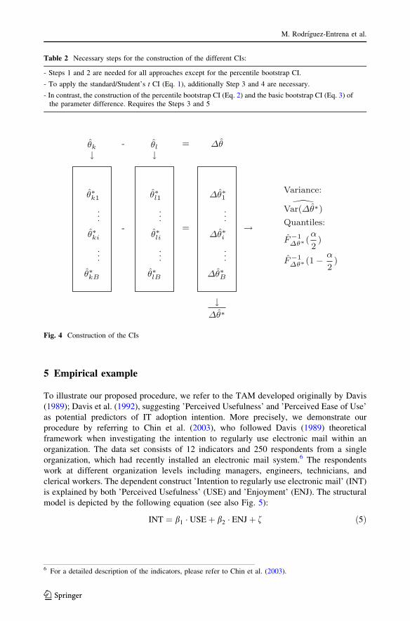
5 Empirical example
To illustrate our proposed procedure, we refer to the TAM developed originally by Davis
(1989); Davis et al. (1992), suggesting ’Perceived Usefulness’ and ’Perceived Ease of Use’
as potential predictors of IT adoption intention. More precisely, we demonstrate our
procedure by referring to Chin et al. (2003), who followed Davis (1989) theoretical
framework when investigating the intention to regularly use electronic mail within an
organization. The data set consists of 12 indicators and 250 respondents from a single
organization, which had recently installed an electronic mail system.6 The respondents
work at different organization levels including managers, engineers, technicians, and
clerical workers. The dependent construct ’Intention to regularly use electronic mail’ (INT)
is explained by both ’Perceived Usefulness’ (USE) and ’Enjoyment’ (ENJ). The structural
model is depicted by the following equation (see also Fig. 5):
INT ¼ b1 � USEþ b2 � ENJþ f ð5Þ
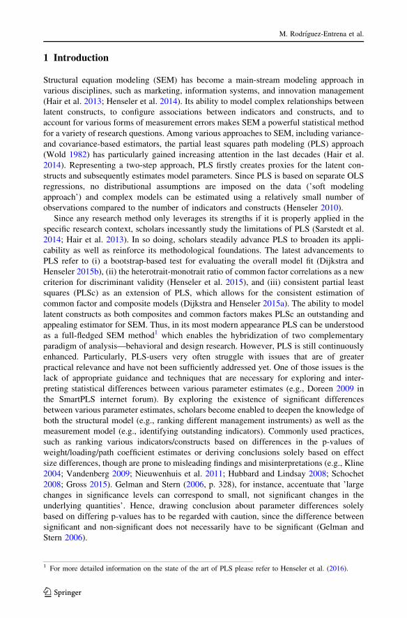
Table 2 Necessary steps for the construction of the different CIs:
- Steps 1 and 2 are needed for all approaches except for the percentile bootstrap CI.
- To apply the standard/Student’s t CI (Eq. 1), additionally Step 3 and 4 are necessary.
- In contrast, the construction of the percentile bootstrap CI (Eq. 2) and the basic bootstrap CI (Eq. 3) ofthe parameter difference. Requires the Steps 3 and 5
θ∗k1
...
θ∗ki
...
θ∗kB
-
θ∗l1
...
θ∗li
...
θ∗lB
=
Δθ∗1
...
Δθ∗i
...
Δθ∗B
→
Variance:
Var(Δθ∗)Quantiles:
F −1Δθ∗ (
α
2)
F −1Δθ∗ (1 − α
2)
θk
↓- θl
↓= Δθ
↓Δθ∗
Fig. 4 Construction of the CIs
6 For a detailed description of the indicators, please refer to Chin et al. (2003).
M. Rodrıguez-Entrena et al.
123

Following Chin et al. (2003), all constructs are modeled as common factors. While USE is
measured by six indicators, both ENJ and INT are measured by three indicators each. All
indicators are on a seven-point Likert scale.
Using our proposed procedure for statistically testing the difference between two
parameter estimates, we seek to answer whether USE (extrinsic motivation) has a statis-
tically different impact on INT than ENJ (intrinsic motivation) (H0: b1 ¼ b2). Since this
model was originally estimated by traditional PLS but represents a common factor model,
we used both approaches PLS and PLSc (Dijkstra and Henseler 2015a) for model esti-
mation.7 The analysis eventually leads to the following estimated path coefficients: b1 ¼0:517 and b2 ¼ 0:269 for the model estimation with PLS and b1 ¼ 0:507 and b2 ¼ 0:313for the model estimation with PLSc.
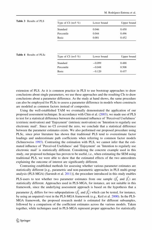
The 95 % CIs derived from the bootstrap procedure with 5000 draws (see Sect. 3) are
displayed in Tables 3 and 4. Since they do not contain the zero with regard to the esti-
mation using PLS, we infer that both path coefficient estimates (b1 and b2) are significantlydifferent. With regard to the estimation with PLSc, all CIs cover the zero. We, therefore,
conclude that the difference between the two path coefficient estimates (b1 and b2) is notstatistically significant.8 Hence, if the underlying measurement models are conceptualized
as composites (i.e., model estimation using PLS), the null hypothesis of no parameter
difference (H0: b1 ¼ b2) has to be rejected. If the measurement models, on the other hand,
are conceptualized as common factors (i.e., model estimation with PLSc), there is not
enough evidence against the null hypothesis.
6 Discussion
The purpose of this paper is to provide a practical guideline as well as the technical
background for assessing the statistical difference between two parameter estimates in
SEM using PLS. This guideline is intended to be used to test a parameter difference based
on the parameter estimates and the bootstrap distribution. The input required for the
proposed methodological procedure directly builds on the output of the most popular
variance-based SEM statistical software packages such as ADANCO or SmartPLS. The
methodological procedure serves as functional toolbox that can be considered as a natural
PerceivedUse
Enjoyment
Intention toregularly useelectronic
β1
β2
Fig. 5 Structural model of thereduced TAM
7 As outer weighting scheme we used mode A and the factorial scheme was used as inner weightingscheme.8 As PLSc path coefficient estimates are known to have a larger standard deviation compared to PLSestimates (Dijkstra and Henseler 2015a), it is not surprising that PLSc produced larger CIs than PLS.
Assessing statistical differences between parameters...
123
extension of PLS. As it is common practice in PLS to use bootstrap approaches to draw
conclusions about single parameters, we use these approaches and the resulting CIs to draw
conclusions about a parameter difference. As the study at hand shows, the same procedure
can also be employed for PLSc to assess a parameter difference in models where constructs
are modeled as common factors instead of composites.
Using the well-established TAM we eventually demonstrated the application of our
proposed assessment technique. In accordance with Chin et al. (2003), we made use of PLS
to test for a statistical difference between the estimated influence of ’Perceived Usefulness’
(extrinsic motivation) and ’Enjoyment’ (intrinsic motivation) on ’Intention to regularly use
electronic mail’. Since no CI covered the zero, we conclude that a statistical difference
between the parameter estimates exists. We also performed our proposed procedure using
PLSc, since prior literature has shown that traditional PLS tend to overestimate factor
loadings and underestimate path coefficients when referring to common factor models
(Schneeweiss 1993). Contrasting the estimation with PLS, we cannot infer that the esti-
mated influence of ’Perceived Usefulness’ and ’Enjoyment’ on ’Intention to regularly use
electronic mail’ is statistically different. Considering the concrete example used in this
study, our proposed technique has proven to be useful, i.e., when estimating the SEM using
traditional PLS, we were able to show that the estimated effects of the two antecedents
explaining the outcome of interest are significantly different.
Contrasting established methods for assessing whether various parameter estimates are
statistically different [e.g., parametric and non-parametric approaches in PLS multi-group
analysis (PLS-MGA) (Sarstedt et al. 2011)], the procedure introduced in this study enables
PLS-users to test whether two parameter estimates from one sample (b1
k and b1
l ) are
statistically different. Approaches used in PLS-MGA, for instance, are not suitable in this
framework, since the underlying assessment approach is based on the hypothesis that a
parameter bk differs for two subpopulations (b1
k and b2
k) which can be tested, for instance,
by using an unpaired t-test in the PLS-MGA framework (e.g., Keil et al. 2000). In the PLS-
MGA framework, the proposed research model is estimated for different subsamples,
followed by a comparison of the coefficient estimates across the various models. Taken
together, while techniques used in PLS-MGA represent proper approaches for statistically
Table 3 Results of PLSType of CI (a=5 %) Lower bound Upper bound
Standard 0.046 0.450
Percentile 0.044 0.496
Basic 0.001 0.452
Table 4 Results of PLScType of CI (a=5 %) Lower bound Upper bound
Standard -0.099 0.488
Percentile -0.048 0.508
Basic -0.120 0.437
M. Rodrıguez-Entrena et al.
123

assessing the difference between the same parameter estimate but for different subsamples
(H0: bik ¼ bjk, where i and j refer to the different subpopulations and k to the parameter
tested), the procedure proposed in the study at hand represents the first choice when
assessing the difference between two parameter estimates derived from the same sample
(H0: bik ¼ bil, where i refers to the population, and k and l to the parameters tested).
Although the present study only considered path coefficient estimates while testing for
differences, the proposed approach might also be performed with regard to other parameter
estimates, such as weights, factor-loadings, or cross-loadings. Thus, testing for statistically
significant differences between factor-loading and cross-loading estimates, for instance,
might be a promising approach for evaluating discriminant validity (e.g., Hair et al. 2011;
Henseler et al. 2009). Analysing whether estimated weights are significantly different
might further be useful for identifying key indicators of composites. Furthermore, while
the study at hand focused on explanative analysis—which still tends to be the main-stream
in business research, the identification of statistical differences among parameter estimates
might also become a standard procedure for predictive-analysis, which is becoming more
and more pronounced in business and social science researcher (Carrion et al. 2016).
7 Limitations and future research
Though we were able to introduce a diagnostic procedure for statistically assessing the
differences between two parameter estimates, the study at hand is not without limitations.
Firstly, we only considered the difference between one pair of parameter estimates. We,
thus, recommend future research to develop procedures for testing more than two
parameter estimates, following two potential approaches: (i) performing several single tests
and adjust the assumed level of significance (e.g., using the Bonferroni correction) (Rice
1989), or (ii) performing a joint test, similar to a F-test in regression analysis.
Secondly, the procedure proposed in this study solely makes use of basic bootstrap
approaches when calculating the required CIs. Therefore, scholars might also consider
more sophisticated techniques, such as studentized, bias-corrected, tilted, balanced, ABC,
antithetic, or m-out-of-n bootstrap techniques.
Thirdly, more general, scholars might in more detail investigate the performance and
limitations of the various bootstrap procedures when using PLS and PLSc, in particular for
small sample sizes, i.e., by a simulation study.
Acknowledgments This research has been funded by the Regional Government of Andalusia (Junta deAndalucıa) through the research Project RTA2013-00032-00-00 (MERCAOLI) which is co-financed by theINIA (National Institute of Agricultural Research) and Ministerio de Economıa y Competitividad as well asby the European Union through the ERDF—European Regional Development Fund 2014–2020 ProgramaOperativo de Crecimiento Inteligente. The first author acknowledges the support provided by the IFAPA—Andalusian Institute of Agricultural Research and Training and the European Social Fund (ESF) within theOperative Program of Andalusia 2007–2013 through a post-doctoral training programme.
Open Access This article is distributed under the terms of the Creative Commons Attribution 4.0 Inter-national License (http://creativecommons.org/licenses/by/4.0/), which permits unrestricted use, distribution,and reproduction in any medium, provided you give appropriate credit to the original author(s) and thesource, provide a link to the Creative Commons license, and indicate if changes were made.
Assessing statistical differences between parameters...
123
References
Carrion, G.C., Henseler, J., Ringle, C.M., Roldan, J.L.: Prediction-oriented modeling in business research bymeans of PLS path modeling: introduction to a JBR special section. J. Bus. Res. 69(10), 4545–4551(2016)
Chin, W.W., Marcolin, B.L., Newsted, P.R.: A partial least squares latent variable modeling approach formeasuring interaction effects: Results from a Monte Carlo simulation study and an electronic-mailemotion/adoption study. Inf. Syst. Res. 14(2), 189–217 (2003)
Davis, F.D.: Perceived usefulness, perceived ease of use, and user acceptance of information technology.MIS Quari. 13(3), 319–340 (1989)
Davis, F.D., Bagozzi, R.P., Warshaw, P.R.: Extrinsic and intrinsic motivation to use computers in theworkplace. J. Appl. Soc. Psychol. 22(14), 1111–1132 (1992)
Davison, A.C., Hinkley, D.V.: Bootstrap Methods and Their Application, vol. 1. Cambridge UniversityPress, Cambridge (1997)
Dijkstra, T.K., Henseler, J.: Consistent and asymptotically normal PLS estimators for linear structuralequations. Comput. Stat. Data Anal. 81, 10–23 (2015a)
Dijkstra, T.K., Henseler, J.: Consistent partial least squares path modeling. MIS Quart. 39(2), 297–316(2015b)
Doreen: Significance testing of path coefficients within one model. SmartPLS online forum comment. http://forum.smartpls.com/viewtopic.php?f=5&t=956&p=2649&hilit=testing?significant?differences#p2649 (2009)
Eberl, M., Schwaiger, M.: Corporate reputation: disentangling the effects on financial performance. Eur.J. Mark. 39(7/8), 838–854 (2005)
Efron, B., Tibshirani, R.J.: An Introduction to the Bootstrap. CRC Press, Boca Raton (1994)Eggert, A., Henseler, J., Hollmann, S.: Who owns the customer? Disentangling customer loyalty in indirect
distribution channels. J. Suppl. Chain Manag. 48(2), 75–92 (2012)Gelman, A., Stern, H.: The difference between significant and not significant is not itself statistically
significant. Am. Stat. 60(4), 328–331 (2006)Gross, J.H.: Testing what matters (if you must test at all): A context-driven approach to substantive and
statistical significance. Am. J. Polit. Sci. 59(3), 775–788 (2015)Hair, J.F., Ringle, C.M., Sarstedt, M.: PLS-SEM: indeed a silver bullet. J. Mark. Theory Pract. 19(2),
139–152 (2011)Hair, J.F., Ringle, C.M., Sarstedt, M.: Editorial-partial least squares structural equation modeling: rigorous
applications, better results and higher acceptance. Long Range Plan. 46(1–2), 1–12 (2013)Hair, F.J.J., Sarstedt, M., Hopkins, L., Kuppelwieser, G.V.: Partial least squares structural equation mod-
eling (PLS-SEM): an emerging tool in business research. Eur. Bus. Rev. 26(2), 106–121 (2014)Henseler, J.: On the convergence of the partial least squares path modeling algorithm. Comput. Stat. 25(1),
107–120 (2010)Henseler, J.: PLS-MGA: a non-parametric approach to partial least squares-based multi-group analysis. In:
Gaul, W., Geyer-Schulz, A., Schmidt-Thieme, L., Kunze, J. (eds.) Challenges at the Interface of DataAnalysis, Computer Science, and Optimization, pp. 495–501. Springer, New York (2012)
Henseler, J., Dijkstra, T.K.: ADANCO 2.0. http://www.composite-modeling.com (2015)Henseler, J., Ringle, C.M., Sinkovics, R.R.: The use of partial least squares path modeling in international
marketing. Adv. Int. Mark. 20, 277–320 (2009)Henseler, J., Ringle, C.M., Sarstedt, M.: A new criterion for assessing discriminant validity in variance-
based structural equation modeling. J. Acad. Mark. Sci. 43(1), 115–135 (2015)Henseler, J., Hubona, G., Ray, P.A.: Using PLS path modeling in new technology research: updated
guidelines. Ind. Manag. Data Syst. 116(1), 2–20 (2016)Henseler, J., Dijkstra, T.K., Sarstedt, M., Ringle, C.M., Diamantopoulos, A., Straub, D.W., Ketchen, D.J.,
Hair, J.F., Hult, G.T.M., Calantone, R.J.: Common beliefs and reality about PLS: comments on Ronkkoand Evermann (2013). Org. Res. Methods 17(2), 182–209 (2014)
Hubbard, R., Lindsay, R.M.: Why p values are not a useful measure of evidence in statistical significancetesting. Theory Psychol. 18(1), 69–88 (2008)
Keil, M., Tan, B.C., Wei, K.K., Saarinen, T., Tuunainen, V., Wassenaar, A.: A cross-cultural study onescalation of commitment behavior in software projects. Mis Quart. 24(2), 299–325 (2000)
Kline, R.B.: Beyond significance testing: reforming data analysis methods in behavioral research. Am.Psychol. Assoc. 10(4), 713–716 (2004)
McIntosh, C.N., Edwards, J.R., Antonakis, J.: Reflections on partial least squares path modeling. Org. Res.Methods p. 1094428114529165 (2014)
M. Rodrıguez-Entrena et al.
123

Nieuwenhuis, S., Forstmann, B.U., Wagenmakers, E.J.: Erroneous analyses of interactions in neuroscience:a problem of significance. Nat. Neurosci. 14(9), 1105–1107 (2011)
Rice, W.R.: Analyzing tables of statistical tests. Evolution 43(1), 223–225 (1989)Ringle, C., Wende, S., Becker, J.M.: SmartPLS 3. SmartPLS GmbH, Boenningstedt (2015)Sarstedt, M., Henseler, J., Ringle, C.M.: Multigroup analysis in partial least squares (PLS) path modeling:
alternative methods and empirical results. Adv. Int. Mark. 22(1), 195–218 (2011)Sarstedt, M., Ringle, C.M., Hair, J.F.: PLS-SEM: Looking back and moving forward. Long Range Plan.
47(3), 132–137 (2014)Schneeweiss, H.: Consistency at Large in Models with Latent Variables. Elsevier, Amsterdam (1993)Schochet, P.Z.: Guidelines for multiple testing in impact evaluations of educational interventions. final
report. Mathematica Policy Research, Inc (2008)Vandenberg, R.J.: Statistical and Methodological Myths and Urban Legends: Doctrine, Verity and Fable in
the Organizational and Social Sciences. Taylor & Francis, New York (2009)Wehrens, R., Putter, H., Buydens, L.M.: The bootstrap: a tutorial. Chemometr. Intell. Lab. Syst. 54(1),
35–52 (2000)Wold, H.: Soft modeling: The basic design and some extensions. In: Joreskog, K.G., Wold, H. (eds.)
Systems Under Indirect Observations, Part II, pp. 1–54. North-Holland, Amsterdam (1982)
Assessing statistical differences between parameters...
123