Embed Size (px)
Citation preview
1
ARTICLE TITLE: Wind-Induced Vibrations
AUTHORS NAME: Tracy Kijewski, Fred Haan, Ahsan Kareem
AUTHORS AFFILIATION: NatHaz Modeling Laboratory, Department of Civil Engineering and Geological Sciences, University of Notre Dame
AUTHOR ADDRESS: University of Notre Dame, 156 Fitzpatrick Hall, Notre Dame, IN, 46556 USA
INTRODUCTION
As modern structures move toward taller and more flexible designs, the problems of wind effects
on structures -- those compromising structural integrity and those inducing human discomfort--
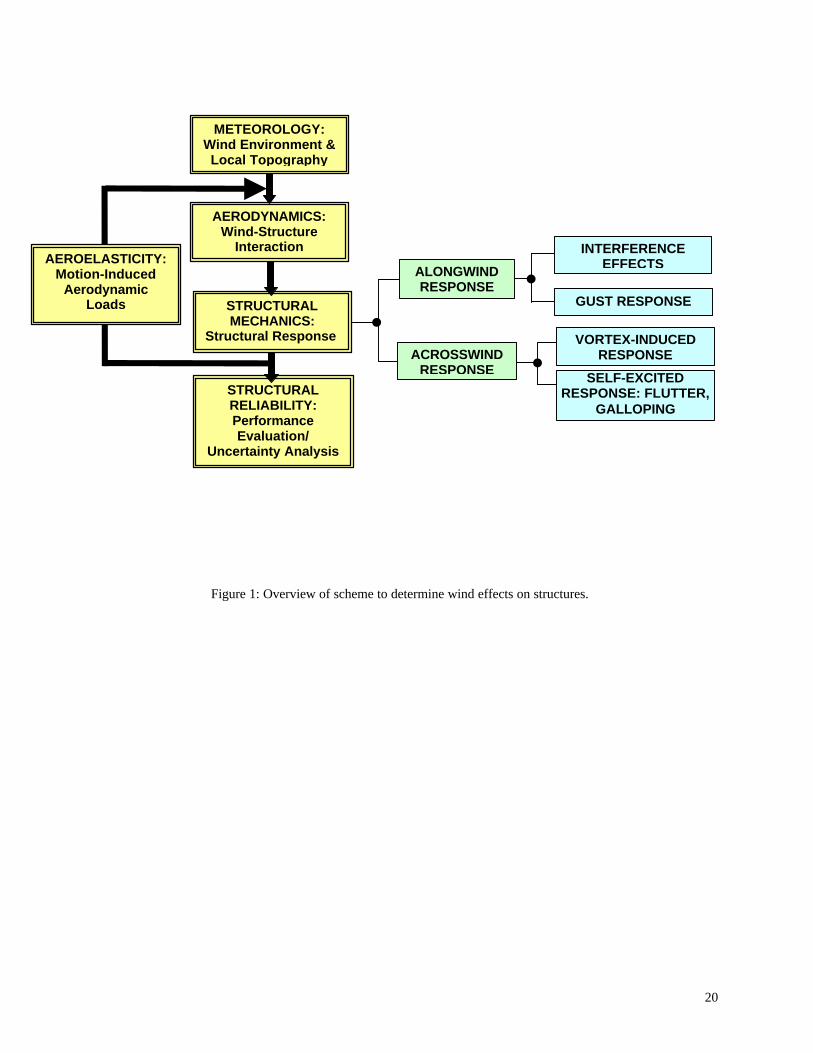
have become increasingly apparent. To fully address this problem, a diverse collection of
contributions must be considered, as illustrated in Figure 1. It is the complexity and uncertainty
of the wind field and its interaction with structures that necessitates such an interdisciplinary
approach, involving scientific fields such as meteorology, fluid dynamics, statistical theory of
turbulence, structural dynamics, and probabilistic methods. The following sections will describe
the contributions from each of these areas, beginning with a description of the wind field
characteristics and the resulting wind loads on structures. Subsequent sections will then address
procedures for determining wind-induced response, including traditional random vibration theory
and code-based approximations, with an example to illustrate the application of both approaches.
The treatment of wind effects on structures will conclude with a discussion of aeroelastic effects,
wind tunnel testing, and the evolving numerical approaches. <insert Figure 1 near here>
WIND CHARACTERISTICS
Civil engineering structures are immersed in the earth’s atmospheric boundary layer, which is
characterized by the earth’s topographic features, e.g., surface roughness. The most common
2
description of the wind velocity within this boundary layer superimposes a mean wind
component, described by a mean velocity profile, with a fluctuating velocity component. The
vertical variation of the mean wind velocity, U , can be represented by a logarithmic
relationship, or by a power law given as:
( )α
=
refref z
zUzU (1)
where refz is the reference height, refU is the mean reference velocity, and α is a constant that
varies with the roughness of the terrain, with specific values defined in fundamental texts.
The fluctuating wind field is characterized by temporal averages, variances of velocity
components, probabilities of exceedance, energy spectra, associated length scales, and space-
time correlations. One important measure is the total energy of the wind fluctuations, expressed
as the standard deviation of the velocity fluctuations normalized by the mean wind velocity, and
referred to as turbulence intensity. The energy spectra describe the distribution of energy at each
frequency, whereas the space-time correlation describes the degree to which velocity
fluctuations are correlated in space and/or time. A measure of the average size of turbulent
eddies, the length scale, can be then estimated by integrating velocity cross-correlation functions.
WIND LOADS ON STRUCTURES
Just as the most elementary description of the velocity of the oncoming wind field superimposes
a mean component, )(zU , increasing with height according to the power law given in Eq. 1,
with a randomly fluctuating component, u(z,t), the oncoming wind will impose loads on the
structure that vary both spatially and temporally. The fluctuating wind velocity translates directly
3
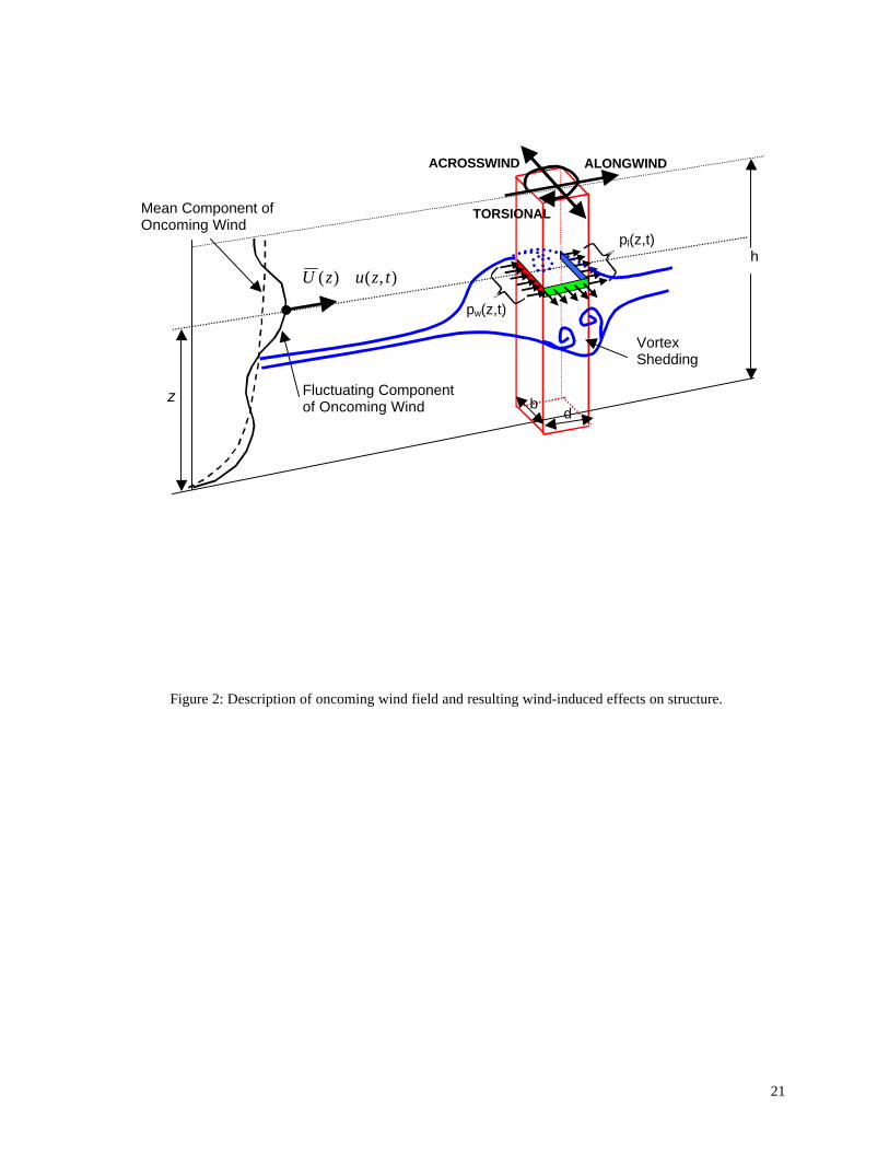
into fluctuating positive pressures (pw (z, t)) distributed across the building’s windward face, as
shown in Figure 2. Corresponding negative pressures, pl (z, t), result on the leeward face of the
structure. <Figure 2 near here>
Upon impacting the windward face, the wind is then deflected around the structure and
accelerated such that it cannot negotiate the sharp corners and thus separates from the building,
leaving a region of high negative pressure, also shown in Figure 2. This separated flow forms a
shear layer on each side, and subsequent interaction between the layers results in the formation
of discrete vortices, which are shed alternately. This region is generally known as the wake
region.
The three dimensional simultaneous loading of the structure due to its interaction with the wind
results in three structural response components, illustrated in Figure 2. The first, termed the
alongwind component, primarily results from pressure fluctuations in the approach flow, leading
to a swaying of the structure in the direction of the wind. The acrosswind component constitutes
a swaying motion perpendicular to the direction of the wind and are introduced by side-face
pressure fluctuations primarily induced by the fluctuations in the separated shear layers, vortex
shedding and wake flow fields. The final torsional component results from imbalances in the
instantaneous pressure distribution on the building surfaces. These wind load effects are further
amplified on asymmetric buildings as a consequence of inertial coupling in the building
structural system.
As the wind pressures vary spatially over the face of the structure, there is the potential for
regions of high localized pressures, of particular concern for the design of cladding systems;

4
however, it is their collective effect that results in the integral loads used for the design of the
structural system, which will be of primary interest in this discussion.
Since the alongwind motion primarily results from the fluctuations in the approach flow, its load
effects have been successfully estimated using quasi-steady and strip theories, which imply that
the fluctuating pressure field is linearly related to the fluctuating velocity field at any level on the
building. Although the alongwind response may also include interference effects due to the
buffeting of the structure by the wake of upstream obstacles, it is the gust response due to the
oncoming wind that is primarily considered. Thus, the aerodynamic loads, F (t), considering only
this component, are expressed in terms of velocity fluctuations as
( ) )(2/1)(2/1)( 22tuUACUACtuUACtF DDD ρρρ +≈+= (2)
in which ρ = air density, A = projected area of the structure loaded by the wind, and DC = drag
coefficient. This expression is approximated by ignoring the generally small term containing the
square of the fluctuating velocity.
The preceding expression implicitly assumes that the velocity fluctuations approaching a
structure are fully correlated over the entirety of the structure. This assumption may be valid for
very small structures, but fails to hold for structures with larger spatial dimensions and leads to
overestimation of loads. In this case, the effect of imperfect correlation of wind fluctuations is
introduced conveniently through an aerodynamic admittance function. As this loading scenario is
described relatively easily in the frequency domain, Eq. 2 is accordingly transformed and the
aerodynamic admittance, χ2(f), is introduced
( ) ( ) ( ) )(22 fSfCfS uDF χρ= (3)
5
where )( fS F , )( fSu = power spectral density (PSD) of wind loads and wind fluctuations,
respectively. Ideally, )(2 fχ not only represents the lack of correlation in the approach flow, but
it also captures any departure from quasi-steady theory that may result from complex nonlinear
interactions between the fluctuating wind and the structure. The transformation of wind velocity
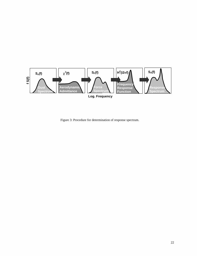
fluctuations to wind force fluctuations is illustrated in the frequency domain in Figure 3. For
simple rectangular plates and prisms, both experimental and theoretical information concerning
)(2 fχ is available. For typical buildings that are aerodynamically bluff, one needs to resort to
wind tunnel tests to directly obtain the PSD of the aerodynamic force. Alternatively, one can
invoke the strip and quasi-steady theories with appropriate correlation structure of the
approaching flow field to estimate )(2 fχ and hence )( fSF ; however, this may introduce some
uncertainty in the estimates, as this approach may not fully capture all the features of the wind-
structure interactions.
The approach described above has served as a building block for the “Gust Loading Factor” used
in most building codes. However, the acrosswind and torsional responses cannot be treated in
terms of these gust factors inasmuch as they are induced by the unsteady wake fluctuations,
which cannot be conveniently expressed in terms of the incident turbulence. As a result,
experimentally derived loading functions have been introduced. Accordingly, the acrosswind and
torsional load spectra obtained by synthesizing the surface pressure fields on scale models of
typical building shapes are available in literature. In a recent study, scale models of a variety of
basic building configurations, with a range of aspect ratios, were exposed to simulated urban and
suburban wind fields to obtain mode-generalized loads. These data are available through the
authors’ interactive database at www.nd.edu/~nathaz.
6
WIND-INDUCED RESPONSE: THEORY
In order to derive the structural response from aerodynamic loads, basic random vibration theory
is utilized. The equations of motion of a structure represented by a discretized lumped-mass
system are given by
[ ]{ } [ ]{ } [ ]{ } { })()()()( tFtxtxtx =++ KCM &&& (4)
in which M, C and K = assembled mass, damping and stiffness matrices of the discretized
system, respectively, x is the displacement, and x& and x&& are the first two time derivatives of x,
representing velocity and acceleration, respectively. In general, these equations are derived to
provide two translations and one rotation per story level; however, for the sake of illustration, it
is assumed here that the structure is uncoupled in each direction. By employing the standard
transformation of coordinates, the following modal representation is obtained for one of the
translation directions
)()()(2 2 tPqqq jjjnjjnjj =++ ωωζ &&& (5)
in which { } { })()( tFtP Tjj φ= where [ ]T denotes transpose, φj, jζ and jnjn f )(2)( πω = are the jth
mode shape, modal critical damping ratio and natural frequency, respectively, and q and its
derivatives now represent modal response quantities related to x and its derivatives, respectively,
by { } [ ]{ })()( tqtx jjφ= . The PSD of response, )( rjq
S is given by
( ) )(2)( )(2
)( fSfiHfSj
rj
Pr
jqπ= (6)
{ } [ ]{ }jFT
jP fSfSj
φφ )()( = (7)
7
in which ( )fiH rj π2)(2
is jth-mode frequency response function (FRF). The superscript r indicates
the derivative of response, i.e., r = 0,1,2,3 denotes displacement, velocity, acceleration and jerk.
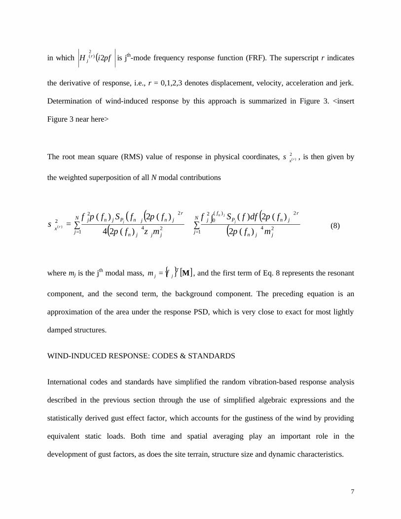
Determination of wind-induced response by this approach is summarized in Figure 3. <insert
Figure 3 near here>
The root mean square (RMS) value of response in physical coordinates, 2)( rx
σ , is then given by
the weighted superposition of all N modal contributions
( ) ( )( )
( )( )∑ ∑
∫+=
= =
N
j
N
j jjn
f rjnPj
jjjn
rjnjnPjnj
x mf
fdffS
mf
ffSf jn
jj
r
1 124
)(0
22
24
22
2
)(2
)(2)(
)(24
)(2)()(
π
πφ
ζπ
ππφσ (8)
where mj is the jth modal mass, { } [ ]MTjjm φ= , and the first term of Eq. 8 represents the resonant
component, and the second term, the background component. The preceding equation is an
approximation of the area under the response PSD, which is very close to exact for most lightly
damped structures.
WIND-INDUCED RESPONSE: CODES & STANDARDS
International codes and standards have simplified the random vibration-based response analysis
described in the previous section through the use of simplified algebraic expressions and the
statistically derived gust effect factor, which accounts for the gustiness of the wind by providing
equivalent static loads. Both time and spatial averaging play an important role in the
development of gust factors, as does the site terrain, structure size and dynamic characteristics.

8
Through the use of random vibration theory, the dynamic amplification of loading or response,
represented by the gust effect factor, can be readily defined. For example, the expected peak
response )(max
ry can be estimated from the RMS value )( ryσ and mean value )(ry by the following
expression, based on the probabilistic description of peak response during an interval T
)()()()(
max ry
rrr gyy σ+= . (9)
The peak factor )(rg varies between 3.5 and 4 and is given by
))ln((2
5772.0))ln((21
1 TfTfg
nn += . (10)
The gust effect factor (GEF) G is then defined as the ratio of the maximum expected response to
the mean response:
)()(
)(
)(max
)(
1r
yrr
r
yg
y
yG
rσ+== . (11)
The RMS response represents the area under the power spectral density of y(r), which can be
described in terms of a background component Q, representing the response due to quasi-steady
effects, and a resonant contribution R to account for dynamic amplification. To simplify the
determination of these terms, international standards provide a series of simplified algebraic
expressions. Typically G is defined in terms of the displacement response
RQIgG Hy++= )0(21 (12)
9
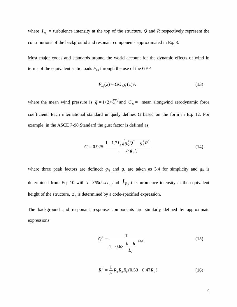
where HI = turbulence intensity at the top of the structure. Q and R respectively represent the
contributions of the background and resonant components approximated in Eq. 8.
Most major codes and standards around the world account for the dynamic effects of wind in
terms of the equivalent static loads Feq through the use of the GEF
AzqGCzF fxeq )()( = (13)
where the mean wind pressure is 22/1 Uq ρ= and fxC = mean alongwind aerodynamic force
coefficient. Each international standard uniquely defines G based on the form in Eq. 12. For
example, in the ASCE 7-98 Standard the gust factor is defined as:
+
++=
zv
RQz
Ig
RgQgIG
7.11
7.11925.0
2222
(14)
where three peak factors are defined: gQ and gv are taken as 3.4 for simplicity and gR is
determined from Eq. 10 with T=3600 sec, and zI , the turbulence intensity at the equivalent
height of the structure, z , is determined by a code-specified expression.
The background and responant response components are similarly defined by approximate
expressions
63.02
63.01
1
++
=
zL
hbQ (15)
)47.053.0(12
Lbhn RRRRR +=β
(16)

10
where b and h are the width and height, respectively, of the structure, shown in Figure 2, and zL
is the integral length scale of turbulence at the equivalent height. The resonant component
involves 4 factors (Rn, Rh, Rb, RL) which are dependent upon the first mode natural frequency,
defined as n1 in ASCE 7-98, and damping ratio, defined in the standard as β, as well as the
dimensions of the structure, the mean wind speed at the equivalent height, zV , and the wind
field’s characteristics. Expressions for these terms may be found in ASCE 7-98.
Following the determination of the gust effect factor, the maximum alongwind displacement Xmax
and RMS accelerations x&&σ may be directly calculated
KGnm
VbhCzzX zfx
211
2
max )2(2
ˆ)()(
πρφ
= (17)
KRIm
VbhCzz z
zfx
X1
2)(85.0)(
ρφσ =&& (18)
where zV̂ is the three second gust at the equivalent height, φ(z) is assumed to be the fundamental
mode shape, m1 is the first mode mass and K is a coefficient representative of the terms resulting
from the integration of the mode shape and wind profile in the determination of the RMS
response. Expressions for these terms are also provided in ASCE 7-98. Note that, in the case of
the acceleration response, background effects are not considered, thus the gust effect factor is not
directly used as defined in Eq. 14. It is instead replaced with a collection of terms analogous to
using a gust effect factor with only a resonant component.
11
WIND-INDUCED RESPONSE: EXAMPLE
To illustrate the determination of wind-induced response by both random vibration theory and by
the code-based procedure, the following example is provided. Table 1 lists the assumed
properties of the structure, which is located in a city center. The basic wind speed, measured as a
3 second gust, at the reference height of 33 ft (10 m) in open terrain, is taken as 90 mph (40.23
m/s). For the sake of brevity, only acceleration response will be provided, considering only the
first mode with an assumed linear mode shape. To further simplify the analysis, the response will
be calculated only at the structure’s full height, at which point the mode shape given in Table 1
would equal unity. <insert Table 1 near here>
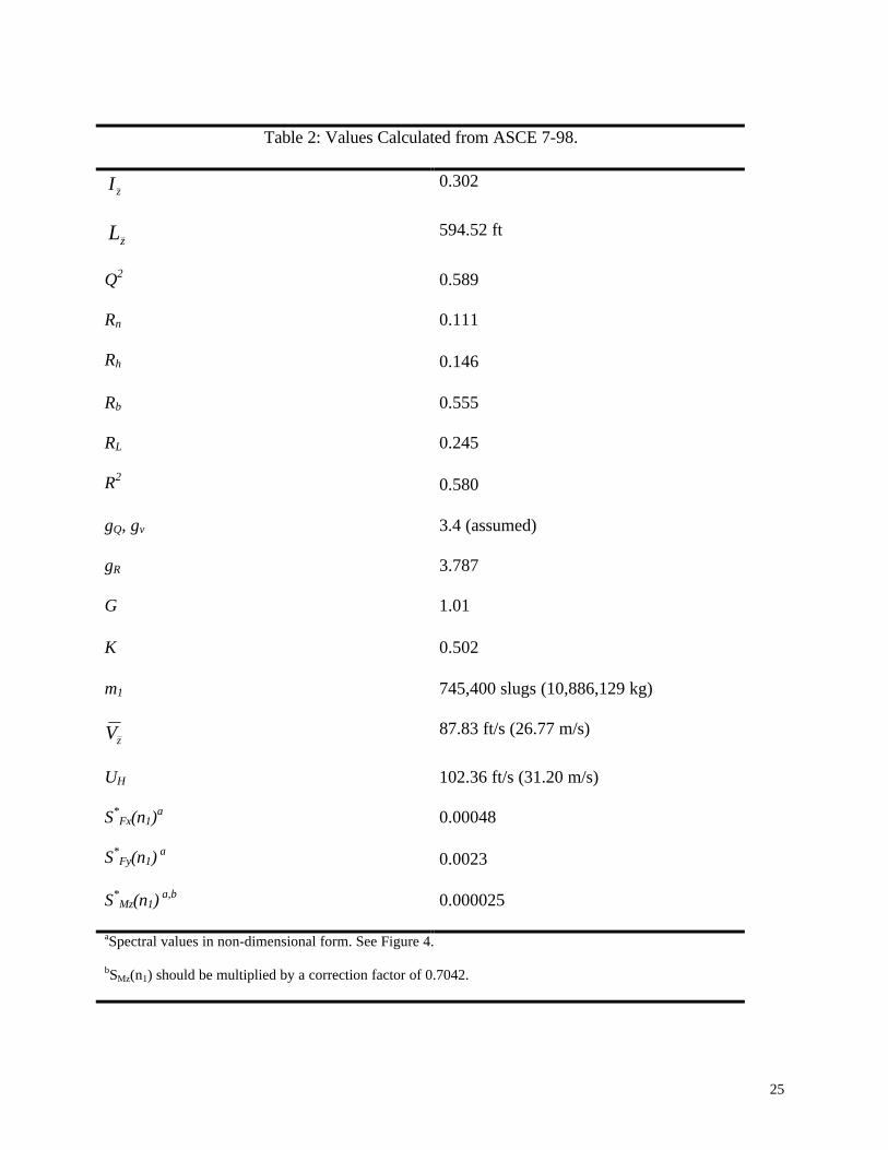
The RMS accelerations in the alongwind direction were first determined in accordance with
ASCE 7-98, by Eq. 18, with all calculated parameters listed in Table 2. Unfortunately, as
discussed previously, acrosswind and torsional responses cannot be determined by the same
analytical procedure and are thus omitted from the ASCE 7 Standard. However, these response
components, as well as the alongwind response, can readily be determined by Eq. 8 with the aid
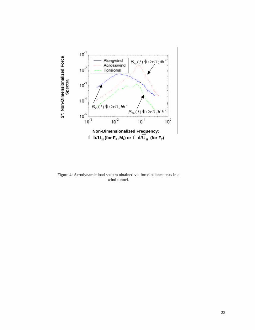
of the wind tunnel data provided in Figure 4. Note that it is common practice to plot these load
spectra in a non-dimensional form, S*, as defined in Figure 4, where HU is the mean wind
velocity at the height of the building, in urban terrain. A power law relationship (Eq. 1) can be
used to translate the reference wind velocity of 90 mph from open terrain at 33 ft (10 m) to urban
terrain at the buiding height. <insert Table 2 and Figure 4 near here>
In the case of acceleration response, r=2 and N=1 in Eq. 8, as only first mode contributions are
considered. Note also that in Eq. 8, mj is defined as the modal mass for the alongwind and
acrosswind directions, taken as the total mass of the building, divided by 3; however, for the
12
torsional response, this modal mass term must be replaced by the first mode mass moment of
inertia determined by: )(12
1 221 dbm + , where d is the depth of the structure as shown in Figure
2. In addition, the torsional analysis requires the multiplication of the spectral density by a
reduction factor to account for the assumption of a constant mode shape inherent in force-
balance experimental measurements.
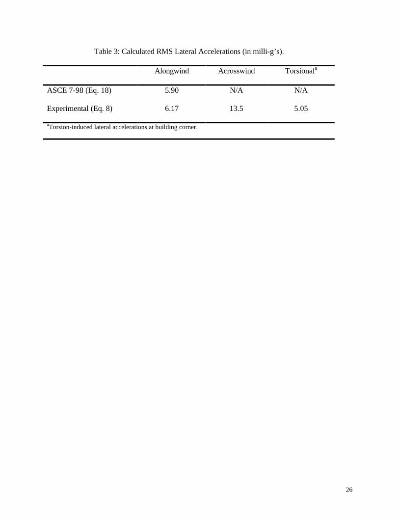
Examining first the properties in Table 2, a comparison of R2 and Q2 reveals that this particular
structure receives nearly equal contributions from the background and resonant components. For
the alongwind response, shown in Table 3, the simplified response estimate given by ASCE 7-98
compares well with the wind tunnel data. Also note that the acrosswind accelerations are twice
that of the alongwind response, illustrating that acrosswind response components have a greater
role in determining the habitability performance of a structure. On the other hand, the structure’s
torsional response is slightly less than the alongwind, which should be no surprise considering
that the structure has no geometric or structural asymmetries and that the loading data from the
wind tunnel was obtained using an isolated building model. <insert Table 3 near here>
SPECIAL TOPICS: AEROELASTIC EFFECTS
The determination of wind-induced loads and response discussed previously did not account for
aeroelastic effects, which can sometimes have significant contributions to the structural response.
Response deformations can alter the aerodynamic forces, thus setting up an interaction between
the elastic response and aerodynamic forces commonly referred to as aeroelasticity. Aeroelastic
contributions to the overall aerodynamic loading are distinguished from other unsteady loads by
recognizing that aeroelastic loads vanish when there is no structural motion. Different types of
13
aeroelastic effects are commonly distinguished from each other. They include vortex-induced
vibration, galloping, flutter, and aerodynamic damping.
As alluded to earlier, aerodynamically bluff cross sections shed vortices at a frequency governed
by the non-dimensional Strouhal number, St :
U
bfSt s= (19)
where sf is the shedding frequency (in Hz). The shedding of vortices generates a periodic
variation in the pressure over the surface of the structure. When the frequency of this variation
approaches one of the natural frequencies of a structure, vortex-induced vibration can occur. The
magnitudes of these vibrations are governed both by the structure’s inherent damping
characteristics and by the mass ratio between the structure and the fluid it displaces. These two
effects are often combined in the Scruton number defined as:
2
4
b
mSc
ρπζ
= (20)
where m is the mass per unit length of the structure.
Vortex-induced vibration is more complex than a mere resonant forcing problem. Nonlinear
interaction between the body motion and its wake results in the “locking in” of the wake to the
body’s oscillation frequency over a larger velocity range than would be predicted using the
Strouhal number. Vortex-induced vibration, therefore, occurs over a range of velocities that
increases as the structural damping decreases.

14
Galloping occurs for structures of certain cross sections at frequencies below those of vortex-
induced vibration. One widely known example of galloping is the large across-wind amplitudes
exhibited by power lines when freezing rain has resulted in a change of their cross section.
Analytically, galloping is considered a “quasi-steady” phenomenon because knowledge of the
static aerodynamic coefficients of a given structure (i.e., mean lift and drag forces on a stationary
model) allows quite reliable prediction of galloping behavior.
Stability of aeroelastic interactions is of crucial importance. The attenuation of structural
oscillations by both structural and aerodynamic damping characterizes stable flow-structure
interactions. In an unstable scenario, the motion-induced loading is further reinforced by the
body motion, possibly leading to catastrophic failure. Such unstable interactions involve
extraction of energy from the fluid flow such that aerodynamic effects cancel structural damping.
Flutter is the term given to this unstable situation, which is a common design issue for long span
bridges.
Depending on the phase of the force with respect to the motion, self-excited forces can be
associated with the displacement, the velocity, or the acceleration of the structure. Because of
these associations, these forces can be thought of as “aerodynamic contributions” to stiffness,
damping, and mass, respectively. In addition to stiffness and damping, aeroelastic effects can
couple modes that are not coupled structurally. Whenever the combined aeroelastic action on
various modes results in negative damping for a given mode, flutter occurs. By means of
structural dynamics considerations and aerodynamic tailoring, flutter must be avoided for the
wind velocity range of interest. Even without resulting in flutter, aeroelastic effects can have a
significant effect on response.
15
SPECIAL TOPICS: WIND TUNNEL TESTING
Despite the obvious advances of computational capabilities over the years, the complexity of the
bluff body fluid-structure interaction problems concerning civil engineering structures has
precluded numerical solutions for the flow around structures. Thus, wind tunnels remain, at this
juncture, the most effective means of estimating wind effects on structures. However, it should
be noted that not all structures require wind tunnel testing. For many conventional structures, for
example, low-rise buildings, code-based estimates may well suffice. Wind tunnel testing may be
necessary, however, when dealing with a novel design or a design for which dynamic and
aeroelastic effects are difficult to anticipate. Examples of such structures include, but are not
limited to, long-span bridges and tall buildings.
Wind tunnel testing of a given structure first involves appropriate modeling of the wind
environment, necessitating various scaling considerations. Geometric scaling is based on the
boundary layer height, the scale of turbulence, and the scale of the surface roughness all
constrained by the size of the wind tunnel itself. Ideally, these lengths should hold to the same
scaling ratio—a performance that can be approached when the boundary layer is simulated over
a long fetch with scaled floor roughness. Dynamic scaling requires Reynolds number equality
between the wind tunnel and the prototype. Without extraordinary measures, this is most often
not possible and must be kept in mind when interpreting results. Velocity scaling is most often
obtained from elastic forces of the structure and inertial forces of the flow. Kinematic scaling
involves appropriate distributions of the mean velocity and turbulence intensity and can be
achieved with flow manipulation in the wind tunnel.
16
Both active and passive means are available for generating turbulent boundary layers. While
active devices such as air jets, flapping vanes and airfoils are capable of generating a wide range
of turbulence parameters, passive devices are cheaper and more efficient to implement. Passive
devices include spires, fences, grids, and floor roughness. Depending on the length and cross
sectional size of the tunnel, surrounding terrain may be modeled as well.
Once an appropriate incident flow has been generated, there are several options for obtaining
aerodynamic load data for the structure of interest. Pressure measurements can be performed on
the surface of a model, forces can be quantified from the base of a lightweight, rigid model, or
forces can be obtained from an aeroelastic model of the structure. Pressure measurements are
capable of quantifying localized loading on a structure’s surface. Issues such as fatigue loads for
cladding panels and panel anchor and glass failure require such localized analysis.
Integrated loads on a structure are often estimated with high-frequency base balances. These
devices are generally integrated into a rotating section of the floor of a wind tunnel. A
lightweight model of the structure is mounted on the balance for measuring wind loads over a
range of incidence angles. The low mass of the model is necessary to ensure that the natural
frequency of the model-balance system is well above any expected wind forcing frequency. A
primary advantage of this approach is that modal force spectra are obtained directly and can be
used in subsequent analytical estimations of building response. As long as the structural
geometry does not change, the forces can be used to analyze the effects of internal structural
design changes without the need for further wind tunnel tests.
Aeroelastic models allow interaction between structural motion and aerodynamic forces. Such
models can be constructed as continuous or discrete models. Continuous models require
17
specialized materials having structural properties matching those of the prototype. Discrete
models are simpler to implement and consist of an internal spine to account for structural
dynamic features with an external cladding that maintains proper geometric scaling with the
prototype. Dynamic response of both buildings and bridges can be estimated utilizing such
models.
SPECIAL TOPICS: NUMERICAL METHODS
With the evolution of computer capabilities, numerical methods have presented another option
for the analysis of fluid-structure interactions. A host of simulation schemes to generate wind
fields and the associated response, in a probabilistic framework, are currently available.
However, these schemes rely on quasi-steady formulations to transform wind fluctuations into
load fluctuations. A welcome departure from the limitations of such approaches is offered by the
field of Computational Fluid Dynamics (CFD), serving as a promising alternative to wind tunnel
testing. One of the more attractive approaches within this area involves the solution of the
Navier-Stokes equations in the Large Eddy Simulation (LES) framework to simulate pressure
fields around structures that convincingly reproduce the experimentally measured pressure-
distributions in both the mean and RMS, as well as replicating the aerodynamic forces and flow
re-attachment features. Coupled with computer-aided flow visualization, which provides visual
animation, this numerical simulation may serve as a useful tool to analyze the evolution of flow
fields around structures and estimate the attendant loads. This approach definitely has merit, and
as computational capacity increases, these schemes will eventually become the methods of
choice.
18
FURTHER READING
American Society of Civil Engineers, 1999, Minimum Design Loads for Buildings and Other
Structures, ASCE7-98. Reston, VA.
Cermak, J.E., 1976, “Aerodynamics of Buildings,” Annual Review of Fluid Mechanics, Vol. 8.
Cermak, J.E., 1987, “Advances in Physical Modeling for Wind Engineering,” Journal of
Engineering Mechanics, Vol. 113, No. 5, pp. 737-756.
Kareem, A., 1987, “Wind Effects on Structures: A Probabilistic Viewpoint,” Probabilistic
Engineering Mechanics, Vol. 2, No. 4, pp. 166-200.
Kareem, A., Kijewski, T. and Tamura, Y., (1999), “Mitigation of Motions of Tall Buildings with
Specific Examples of Recent Applications,” Wind & Structures, Vol. 2, No. 3, pp. 201-251.
Kijewski, T. and Kareem, A., 1998, “Dynamic Wind Effects: A Comparative Study of
Provisions in Codes and Standards with Wind Tunnel Data,” Wind & Structures, Vol. 1, No. 1,
pp. 77-109.
Lutes, L.D. and Sarkani, S., 1997, Stochastic Analysis of Structural and Mechanical Vibrations.
Prentice Hall, New Jersey.
19
Murakami, S., 1998, “Overview of Turbulence Models Applied in CWE-1997,” Journal of Wind
Engineering and Industrial Aerodynamics, Vols. 74-76, pp. 1-24.
Simiu, E. and Scanlan, R., 1996, Wind Effects on Structures. 3rd Ed., John Wiley and Sons, New
York.
Solari, G. and Kareem, A., 1998, “On the Formulation of ASCE7-95 Gust Effect Factor,”
Journal of Wind Engineering & Industrial Aerodynamics, vol. 77 and 78, pp. 673-684.
Sutro, D., 2000, “Into the Tunnel,” Civil Engineering Magazine, June, pp. 37-41.
20
Figure 1: Overview of scheme to determine wind effects on structures.
AEROELASTICITY: Motion-Induced
Aerodynamic Loads
SELF-EXCITED RESPONSE: FLUTTER,
GALLOPING
VORTEX-INDUCED RESPONSE ACROSSWIND
RESPONSE
ALONGWIND RESPONSE
GUST RESPONSE
INTERFERENCE EFFECTS
AERODYNAMICS: Wind-Structure
Interaction
STRUCTURAL MECHANICS:
Structural Response
STRUCTURAL RELIABILITY: Performance Evaluation/
Uncertainty Analysis
METEOROLOGY: Wind Environment & Local Topography
21
Figure 2: Description of oncoming wind field and resulting wind-induced effects on structure.
z
Fluctuating Component of Oncoming Wind
Mean Component of Oncoming Wind
),()( tzuzU +
pw(z,t)
Vortex Shedding
ALONGWIND ACROSSWIND
TORSIONAL
pl(z,t)
d b
h
22
Figure 3: Procedure for determination of response spectrum.
Log. Frequency
Frequency Response Function
Force Spectrum
Aerodynamic Admittance
Gust Spectrum
Response Spectrum
f S
(f)
Su(f) χχ2(f) SF(f) H2(i2ππf) SX(f)
23
Figure 4: Aerodynamic load spectra obtained via force-balance tests in a wind tunnel.
( )222/1/)( dhUffS HFy ρS
*: N
on
-Dim
ensi
on
aliz
ed F
orc
e S
pec
tra
Non-Dimensionalized Frequency:
HUb/f ⋅ (for Fx ,Mz) or HUd/f ⋅ (for Fy)
( )222/1/)( bhUffS HFx ρ( )2222/1/)( hbUffS HMz ρ
24
Table 1: Assumed structural properties.
h 600 ft (182.88 m)
b 100 ft (30.48 m)
d 100 ft (30.48 m)
ρ 0.0024 slugs/ft3 (1.25 kg/m3)
Cfx 1.3
(fn)1:alongwind,acrosswind, torsion 0.2 Hz, 0.2 Hz , 0.35 Hz
ρB: building density 12 lb/ft3 = 0.3727 slugs/ft3 (192.22 kg/m3)
β 0.01
First Mode Shape φ(z)=(z/H)
25
Table 2: Values Calculated from ASCE 7-98.
zI 0.302
zL 594.52 ft
Q2 0.589
Rn 0.111
Rh 0.146
Rb 0.555
RL 0.245
R2 0.580
gQ, gv
gR
3.4 (assumed)
3.787
G 1.01
Κ 0.502
m1 745,400 slugs (10,886,129 kg)
zV 87.83 ft/s (26.77 m/s)
UH 102.36 ft/s (31.20 m/s)
S*Fx(n1)
a 0.00048
S*Fy(n1)
a 0.0023
S*Mz(n1)
a,b 0.000025
aSpectral values in non-dimensional form. See Figure 4.
bSMz(n1) should be multiplied by a correction factor of 0.7042.
26
Table 3: Calculated RMS Lateral Accelerations (in milli-g’s).
Alongwind Acrosswind Torsionala
ASCE 7-98 (Eq. 18) 5.90 N/A N/A
Experimental (Eq. 8) 6.17 13.5 5.05
aTorsion-induced lateral accelerations at building corner.
27
NOTATION A
projected area of building exposed to wind
α
power law exponent
b
width of structure
β
critical damping ratio (ASCE 7-98)
C
structural damping matrix
Cfx
alongwind aerodynamic force coefficient
CD
drag coefficient
d
depth of structure
χχ22
aerodynamic admittance function
f
frequency
fn
natural frequency in Hertz
fs
vortex shedding frequency in Hertz
F
force (or load), in physical coordinates
Feq
equivalent static load
g
peak factor
G
gust effect factor
φ
mode shape
h
height of structure
Η
frequency response function
ΙΗ
turbulence intensity at top of structure
zI
turbulence intensity at equivalent height
j
subscript denoting modal index
28
K
integration constant (ASCE 7-98)
K
structural stiffness matrix
zL
integral length scale of turbulence at equivalent height
M
structural mass matrix
m
structural mass per unit height
mj
jth modal mass
n1
fundamental natural frequency (ASCE 7-98)
N
total number of modal components
P
force (or load), in modal coordinates
pl wind pressure on leeward face of building
pw
wind pressure on windward face of building
Q
background component
q
mean wind pressure
q
modal displacement
q&
modal velocity
q&&
modal acceleration
r
superscript denoting derivative order
R
resonant component
Rn, Rh, Rb, RL
terms for approximation of resonant component (ASCE 7-98)
ρ
air density
ρb
building density
29
Sc
Scruton Number
SF power spectral density of wind loads, in physical coordinates SP
power spectral density of wind loads, in modal coordinates
Sq
power spectral density of response, in modal coordinates
St
Strouhal Number
Su
power spectral density of wind fluctuations
S*
non-dimensionalized load spectra
σ
root mean square
t
time
T
time interval
u
longitudinal velocity fluctuations
U
mean wind velocity
refU
mean wind velocity at reference height
HU
wind velocity at building height
zV
mean wind velocity at equivalent height
zV̂
3 second gust at equivalent height
x
structural displacement, in physical coordinates
x&
structural velocity, in physical coordinates
x&&
structural acceleration, in physical coordinates
Xmax
maximum alongwind displacement (ASCE 7-98)
ωn
natural frequency in rad/sec
y
mean response
ymax
expected peak response
z
vertical position
z
equivalent height
zref
reference height
ζ critical damping ratio

30
[ ]Τ
transpose operator