Ar#ﬁcial)IntelligenceAr#ﬁcial)Intelligence! Dr.!Qaiser!Abbas! Departmentof!Computer!Science!&!IT,!! University!of!Sargodha,!Sargodha,!40100,!Pakistan! [email protected]!

Ar#ficial Intelligence

Dr. Qaiser Abbas Department of Computer Science & IT,

University of Sargodha, Sargodha, 40100, Pakistan [email protected]

Friday 4 December 15 1

1. CONSTRAINT SATISFACTION PROBLEMS

•  We use a factored representa#on for each state: a set of variables, each of which has a value.

•  A problem is solved when each variable has a value that saMsfies all the constraints on the variable. A problem described this way is called a constraint sa#sfac#on problem, or CSP.


1.1. DEFINING CONSTRAINT SATISFACTION PROBLEMS

•  A constraint saMsfacMon problem consists of three components, X, D, and C : –  X is a set of variables, {X1,...,Xn}. –  D is a set of domains, {D1, . . . , Dn}, one for each variable. –  C is a set of constraints that specify allowable combinaMons of values.

–  ⟨scope , rel ⟩, where scope is a tuple of variables that parMcipate in the constraint and rel is a relaMon that defines the values that those variables can take on. •  For example, if X1 and X2 both have the domain values {A,B}, then the constraint saying the two variables must have different values can be wriVen as ⟨(X1, X2), [(A, B), (B, A)]⟩ or as ⟨(X1, X2), X1 ̸= X2⟩.


1.1. DEFINING CONSTRAINT SATISFACTION PROBLEMS

•  To solve a CSP, we need to define a state space and the noMon of a soluMon.

•  Each state in a CSP is defined by an assignment of values to some or all of the variables, {Xi = vi, Xj = vj , . . .}.

•  An assignment that does not violate any constraints is called a consistent or legal assignment.

•  A complete assignment is one in which every variable is assigned, and a solu#on to a CSP is a consistent, complete assignment.

•  A par#al assignment is one that assigns values to only some of the variables.


1.1.1 Example problem: Map coloring

•  Variable X = {WA,NT,Q,NSW,V,SA,T} . •  Domain D = {red , green , blue }. •  Constraint C = {neighboring regions to have disMnct colors}



•  It can be helpful to visualize a CSP as a constraint graph, as shown in Figure 6.1(b). The nodes of the graph correspond to variables of the problem, and a link connects any two variables that parMcipate in a constraint.

•  Since there are nine places where regions border (See Fig 6.1), there are nine constraints as follows: C = {SA ̸= WA, SA ̸= NT, SA ̸= Q, SA ̸= NSW, SA ̸= V, WAd=NT, NT ̸=Q, Qd=NSW, NSW ̸=V}.

•  SA ̸= WA is a shortcut of its formal representaMon (scope, rel) as ⟨(SA, WA), SA ̸= WA⟩, where SA ̸= WA can be fully enumerated in turn as {(red , green ), (red , blue ), (green , red ), (green , blue ), (blue , red ), (blue , green )} .

•  There are many possible soluMons to this problem, such as {WA=red, NT =green, Q=red, NSW =green, V =red, SA=blue, T =red }, can be figuraMvely on next slide.




•  For {SA = blue} in the Australia problem, none of the five neighboring variables can take on the value blue. Without taking advantage of constraint propagaMon, a search procedure would have to consider 35 = 243 assignments for the five neighboring variables; with constraint propagaMon we never have to consider blue as a value, so we have only 25 = 32 assignments to look at, a reducMon of 87%.

1.1.2. Example problem: Job-‐shop scheduling


•  Whenever a task T1 must occur before task T2 , and task T1 takes duraMon d1 to complete, we add an arithmeMc constraint of the form T1 + d1 ≤ T2 . (precedence constraints)

•  We need a disjunc#ve constraint to say that AxleF and AxleB must not overlap in Mme; either one comes first or the other does: (AxleF +10 ≤ AxleB) or (AxleB +10 ≤ AxleF).

•  Read it yourself

1.1.3 Varia#ons on the CSP formalism


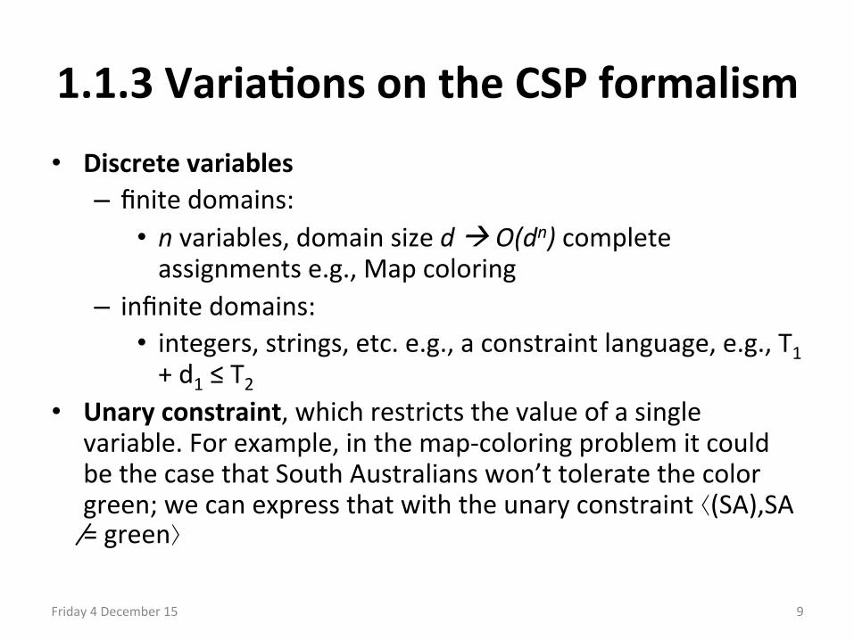
•  Discrete variables –  finite domains:

•  n variables, domain size d à O(dn) complete assignments e.g., Map coloring

–  infinite domains: •  integers, strings, etc. e.g., a constraint language, e.g., T1 + d1 ≤ T2

•  Unary constraint, which restricts the value of a single variable. For example, in the map-‐coloring problem it could be the case that South Australians won’t tolerate the color green; we can express that with the unary constraint ⟨(SA),SA ̸= green⟩



•  A binary constraint relates two variables. For example, SA ̸= NSW is a binary constraint as in Figure 6.1(b).

•  We can also describe higher-‐order constraints, such as asserMng that the value of Y is between X and Z, with the ternary constraint Between(X, Y, Z).

•  A constraint involving an arbitrary number of variables is called a global constraint. One of the most common global constraints is Alldiff, which says that all of the variables involved in the constraint must have different values. Example is cryptarithme#c puzzles. –  Crypto-‐Arithme#c Problem:

•  Crypt-‐ArithmeMc Problems are subsMtuMon problems where leVers represenMng a mathemaMcal operaMon are replaced by unique digits. Like : P L A Y S + W E L L = B E T T E R

•  Where each unique alphabet represents a unique digit from among 0 to 9. So, if the soluMon to this puzzle is to be found, it would be (ater a long computaMon) : 9 7 4 2 6 + 8 0 7 7 = 1 0 5 5 0 3



•  Cryptarithme#c Example: –  The basic rules are :

•  Each unique digit (from 0 to 9) must be replaced by a unique character.

•  The number so formed cannot start with a ZERO. •  SEND + MORE = MONEY

–  SoluMon: •  Total number of Candidate soluMon: 107 x 24 = 160,000,000 for 10 digits, 7 leVers, 2 carry digits and 4 carries involved, however, if M =1, then 80,000,000



1+S+1 = 10 + O à S = 8 + O



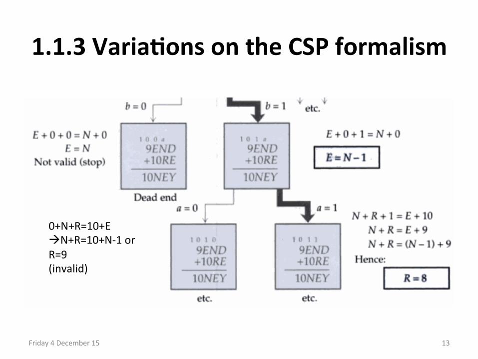
0+N+R=10+E àN+R=10+N-‐1 or R=9 (invalid)



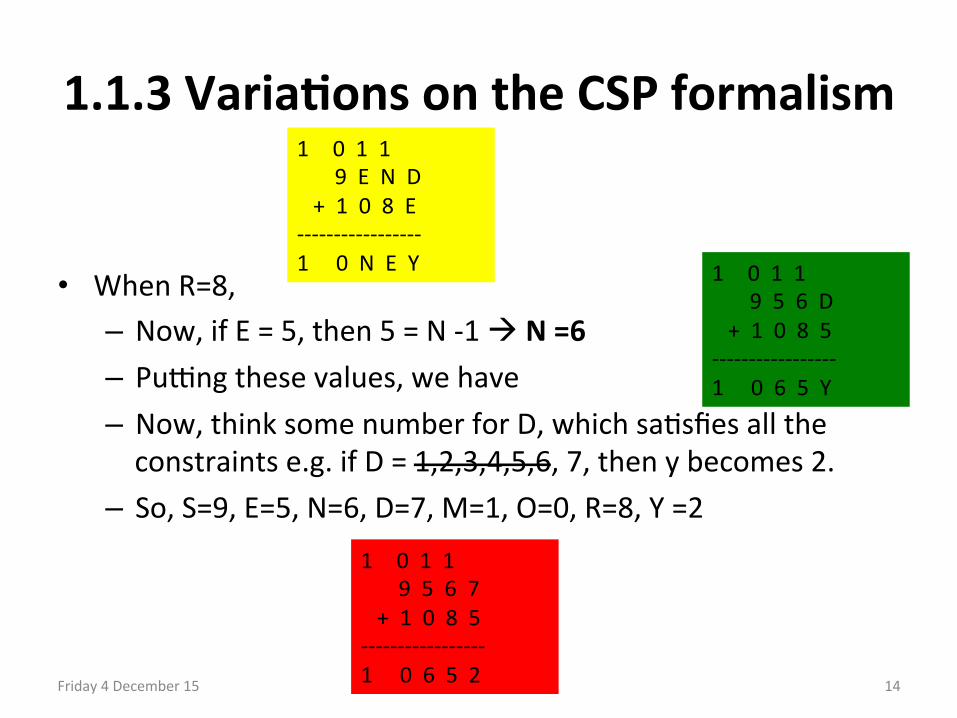
•  When R=8, –  Now, if E = 5, then 5 = N -‐1 à N =6 –  Puung these values, we have –  Now, think some number for D, which saMsfies all the constraints e.g. if D = 1,2,3,4,5,6, 7, then y becomes 2.

–  So, S=9, E=5, N=6, D=7, M=1, O=0, R=8, Y =2

1  0 1 1 9 E N D + 1 0 8 E -‐-‐-‐-‐-‐-‐-‐-‐-‐-‐-‐-‐-‐-‐-‐-‐-‐ 1 0 N E Y 1  0 1 1

9 5 6 D + 1 0 8 5 -‐-‐-‐-‐-‐-‐-‐-‐-‐-‐-‐-‐-‐-‐-‐-‐-‐ 1 0 6 5 Y

1  0 1 1 9 5 6 7 + 1 0 8 5 -‐-‐-‐-‐-‐-‐-‐-‐-‐-‐-‐-‐-‐-‐-‐-‐-‐ 1 0 6 5 2

1.2 BACKTRACKING SEARCH FOR CSPs


•  CSP Standard search formula#on (incremental) –  Let's start with the straighworward approach, then fix it. States are defined by the values assigned so far: •  IniMal state: the empty assignment { } •  Successor funcMon: assign a value to an unassigned

variable that does not conflict with current assignment à fail if no legal assignments

•  Goal test: the current assignment is complete

–  This is the same for all CSPs and it uses depth first search.



•  Variable assignments in all CSPs are commutaMve, i.e., [ WA = red then NT = green ] same as [ NT = green then WA = red ]

•  Backtracking search is used for a depth-‐first search that chooses values for one variable at a Mme and backtracks when a variable has no legal values let to assign.

•  The algorithm is shown in Figure 6.5. It repeatedly chooses an unassigned variable, and then tries all values in the domain of that variable in turn, trying to find a soluMon.

•  If an inconsistency is detected, then BACKTRACK returns failure, causing the previous call to try another value.

•  Part of the search tree for the Australia problem is shown in Figure 6.1 , where we have assigned variables in the order WA, NT , Q, . . ..







•  Improving backtracking efficiency – Which variable should be assigned next (SELECT-‐UNASSIGNED-‐VARIABLE), and in what order should its values be tried (ORDER-‐DOMAIN-‐VALUES)?

– What inferences should be performed at each step in the search (INFERENCE)? •  Can we detect inevitable(unavoidable) failure early?

– When the search arrives at an assignment that violates a constraint, can the search avoid repeaMng this failure?

1.2.1 Variable and value ordering


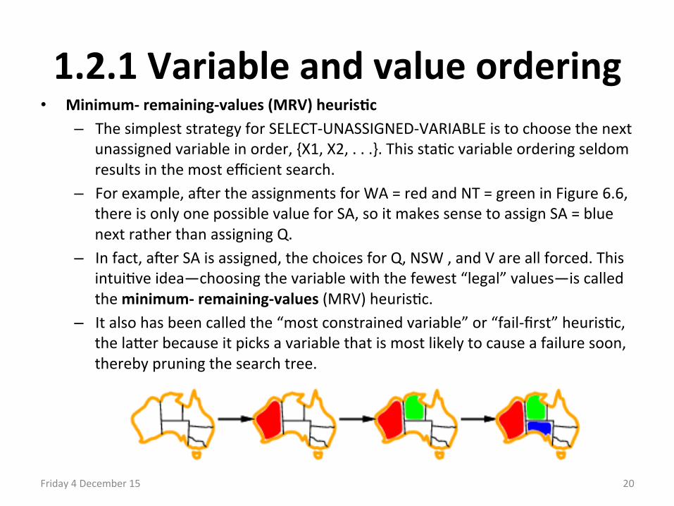
•  Minimum-‐ remaining-‐values (MRV) heuris#c –  The simplest strategy for SELECT-‐UNASSIGNED-‐VARIABLE is to choose the next

unassigned variable in order, {X1, X2, . . .}. This staMc variable ordering seldom results in the most efficient search.

–  For example, ater the assignments for WA = red and NT = green in Figure 6.6, there is only one possible value for SA, so it makes sense to assign SA = blue next rather than assigning Q.

–  In fact, ater SA is assigned, the choices for Q, NSW , and V are all forced. This intuiMve idea—choosing the variable with the fewest “legal” values—is called the minimum-‐ remaining-‐values (MRV) heurisMc.

–  It also has been called the “most constrained variable” or “fail-‐first” heurisMc, the laVer because it picks a variable that is most likely to cause a failure soon, thereby pruning the search tree.



•  Degree heuris#c: –  The MRV heurisMc doesn’t help at all in choosing the first region to color in

Australia, because iniMally every region has three legal colors. –  In this case, the degree heuris#c comes in handy. It aVempts to reduce the

branching factor on future choices by selecMng the variable that is involved in the largest number of constraints on other unassigned variables.

–  In Figure 6.1, SA is the variable with highest degree, 5; the other variables have degree 2 or 3, except for T , which has degree 0.

–  In fact, once SA is chosen, applying the degree heurisMc solves the problem without any false steps—you can choose any consistent color at each choice point and sMll arrive at a soluMon with no backtracking. The MRV heurisMc is usually a more powerful guide, but the degree heurisMc can be useful as a Me-‐breaker.



•  Least-‐constraining-‐value –  Given a variable, choose the least constraining value. The one that rules out the fewest values in the remaining variables.

–  we have generated the parMal assignment with WA = red and NT = green and that our next choice is for Q. Blue would be a bad choice because it eliminates the last legal value let for Q’s neighbor, SA. The least-‐constraining-‐value heurisMc therefore prefers red to blue. In general, the heurisMc is trying to leave the maximum flexibility for subsequent variable assignments.

1.2.2 Interleaving search and inference


•  Forward Checking –  One of the simplest forms of inference is called forward checking. –  Whenever a variable X is assigned, the forward-‐checking process establishes

arc consistency for it: •  for each unassigned variable Y that is connected to X by a constraint, delete from Y ’s domain

any value that is inconsistent with the value chosen for X.

–  Because forward checking only does arc consistency inferences, there is no reason to do forward checking if we have already done arc consistency as a preprocessing step.





















•  Drawback in Forward Checking –  Although forward checking detects many inconsistencies, it does not detect all

of them. The problem is that it makes the current variable arc-‐consistent, but doesn’t look ahead and make all the other variables arc-‐consistent.

–  For example, consider the Figure. It shows that when WA is red and Q is green , both NT and SA are forced to be blue.

–  Forward checking does not look far enough ahead to noMce that this is an inconsistency: NT and SA are adjacent and so cannot have the same value.



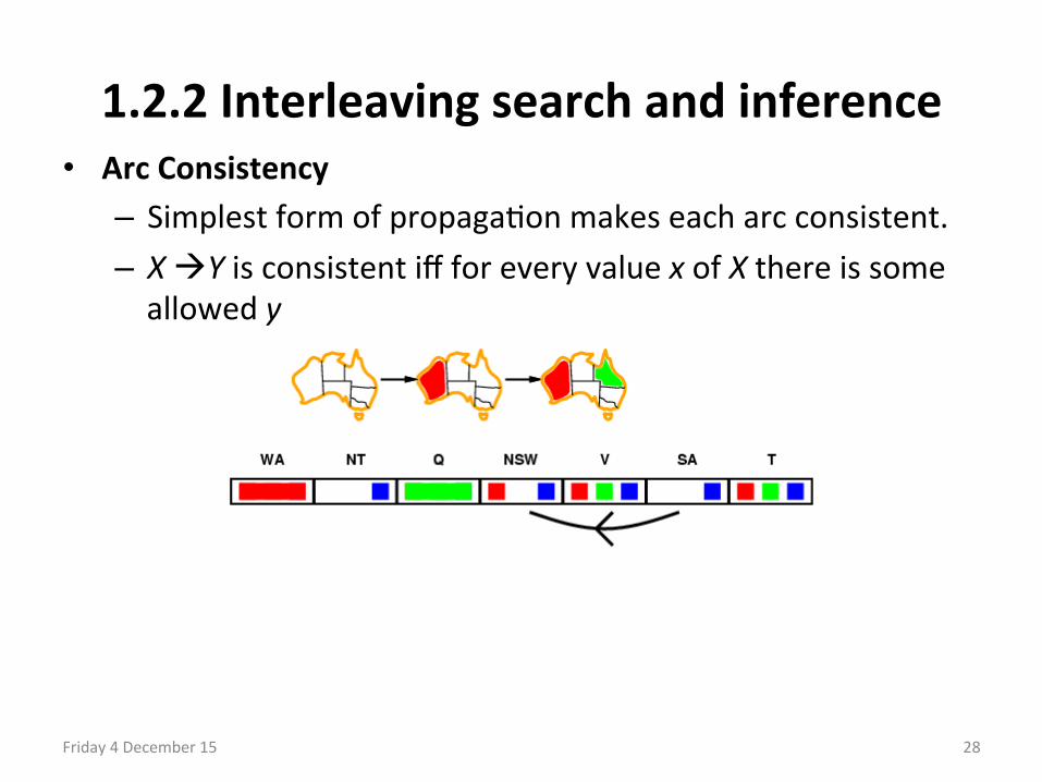
•  Arc Consistency –  Simplest form of propagaMon makes each arc consistent. –  X àY is consistent iff for every value x of X there is some allowed y







–  If X loses a value, neighbors of X need to be rechecked




–  If X loses a value, neighbors of X need to be rechecked –  Arc consistency detects failure earlier than forward checking –  Can be run as a preprocessor or ater each assignment

1.2.3 Intelligent backtracking: Looking backward


•  The BACKTRACKING-‐SEARCH algorithm in Figure 6.5 has a very simple policy for what to do when a branch of the search fails: back up to the preceding variable and try a different value for it. This is called chronological (order as variables occurred) backtracking.

•  Consider what happens when we apply simple backtracking in Figure 6.1 with a fixed variable ordering Q, NSW , V , T , SA, WA, NT . Suppose we have generated the parMal assignment {Q=red,NSW =green,V =blue,T =red}. When we try the next variable, SA, we see that every value violates a constraint. We back up to T and try a new color for Tasmania! Obviously this is silly—recoloring Tasmania cannot possibly resolve the problem with South Australia.

•  A more intelligent approach to backtracking is to backtrack to a variable that might fix the problem—a variable that was responsible for making one of the possible values of SA impossible. To do this, we will keep track of a set of assignments that are in conflict with some value for SA. The set (in this case {Q=red,NSW =green,V =blue,}), is called the conflict set for SA. The backjumping method backtracks to the most recent assignment in the conflict set; in this case, backjumping would jump over Tasmania and try a new value for V . A backjumping algorithm that uses conflict sets defined in this way is called conflict-‐directed backjumping.

1.3 LOCAL SEARCH FOR CSPs


•  Read it yourself

Addi#onal Readings


•  THE STRUCTURE OF PROBLEMS (See SecMon 6.5 ) •  CONSTRAINT PROPAGATION: INFERENCE IN CSPs (See SecMon

6.2 )

Assignment No.6


•  Exercise Numbers: 6.1, 6.5, 6.7, 6.9, 6.16 •  Deadline is the next lecture

Documents

Ar#ﬁcial)IntelligenceAr#ﬁcial)Intelligence! Dr.!Qaiser!Abbas! Departmentof!Computer!Science!&!IT,!! University!of!Sargodha,!Sargodha,!40100,!Pakistan! [email protected]!