Approximation Algorithms Chapter 28: Counting Problems 2003/06/17

Approximation AlgorithmsChapter 28: Counting Problems

2003/06/17

Issues in this chapter

Definitions for counting # solutions– #P, #P-complete, fully polynomial randomized

approximation scheme (FPRAS). Counting DNF solutions Network reliability

Summary

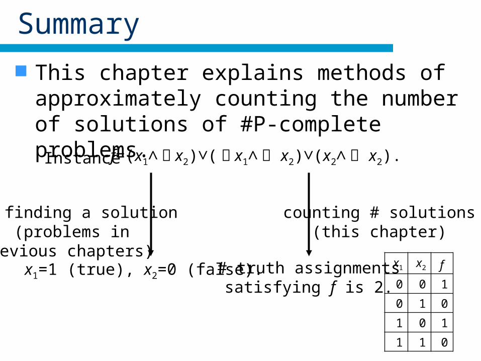
This chapter explains methods of approximately counting the number of solutions of #P-complete problems.

Instance f=(x1∧￢ x2) (∨ ￢ x1∧￢ x2) (∨ x2∧￢ x2).

finding a solution(problems in

previous chapters) x1=1 (true), x2=0 (false). x1 x2 f

0 0 1

0 1 0

1 0 1

1 1 0

counting # solutions(this chapter)

# truth assignmentssatisfying f is 2.

Two major approaches

methods for counting the number of solutions

Markov Chain Monte Carlo Combinatorial Algorithms(not using MCMC)

Counting # truth assignments satisfying a DNF formula

Estimating failure prob. of an undirected network

Topics of this chapter

Definition of #P #P denotes a class of counting problems. We use the following notations for the definition.

– L: a language in NP• all instances satisfying constraints of an NP problem

• L3SAT={(x1∨x1∨x1), (x1∨x2∨￢ x3) (∧ ￢ x1∨x2∨x3), …}

– M: a verifier for L• M((x1∨x1∨x2),((x1, x2)=(1, 1))):

– p: polynomial bounding the length of M’s certificates (y).• p3SAT(|x|)≦c1n≦c2|x| (x: instance, n: # variables, c1, c2: constants).

– f(x): the number of strings y s.t. |y|<p(|x|) and M(x,y) accepts. Such f(x) constitutes the class #P.

Definition of #P-complete

#P-complete intuitively means one of the most intractable counting problems in NP.

f is #P-complete if – f is in #P.– For any g in #P, g is reducible to f .

• There are a transducer R and a function S that are polynomial time computable.

– R(x)∈Lf ⇔ x∈Lg.

– g(x)=S(x, f(R(x)).

#P

f g1

g2

Rg1 Sg1

Rg2 Sg2

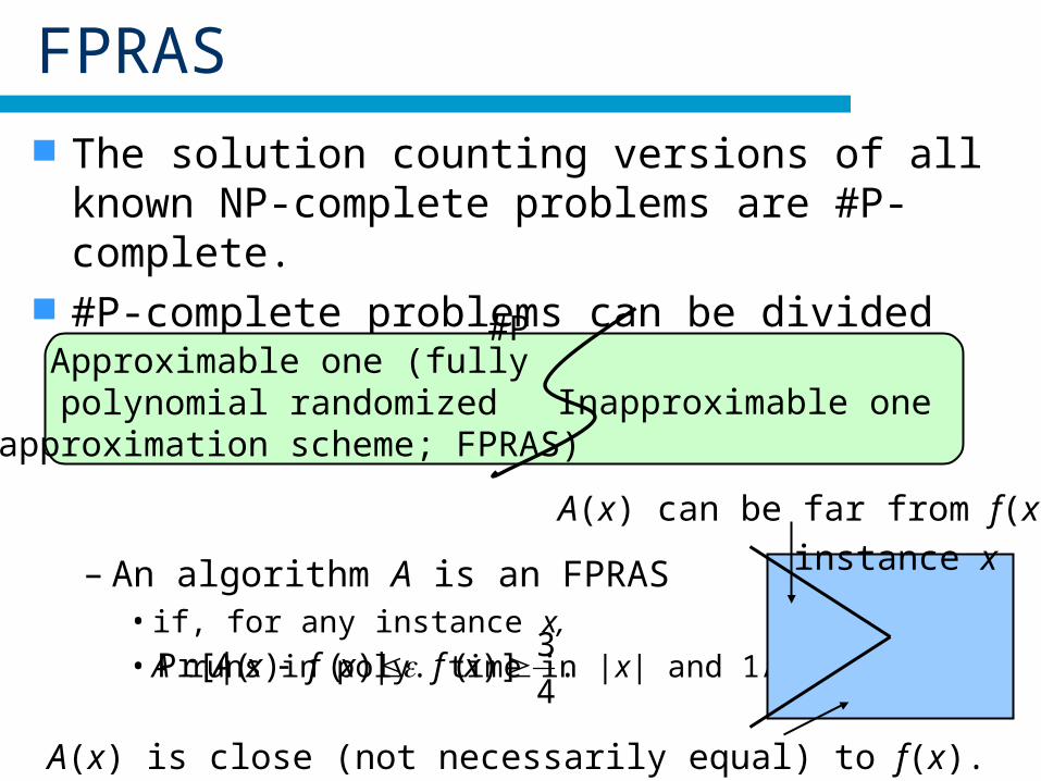
The solution counting versions of all known NP-complete problems are #P-complete.

#P-complete problems can be divided into two.

– An algorithm A is an FPRAS• if, for any instance x,

• A runs in poly. time in |x| and 1/ε, and

#PApproximable one (fullypolynomial randomized

approximation scheme; FPRAS)Inapproximable one

FPRAS

.4

3)]( |)()(Pr[| xfxfxA

instance x

A(x) is close (not necessarily equal) to f(x).

A(x) can be far from f(x).




Counting DNF solutions

Input: – a formula f in disjunctive normal form (DNF) on n

Boolean variables.• E.g., fEX=(x1∧￢ x2) (∨ x2∧ ￢ x3 ) (∨ ￢ x1 ).

Output: – The number of satisfying truth assignments of f.

• Let #f be the number (#fEX is 7).

x1 x2 x3 f

0 0 0 1

0 0 1 1

0 1 0 1

0 1 1 1

x1 x2 x3 f

1 0 0 1

1 0 1 1

1 1 0 1

1 1 1 0

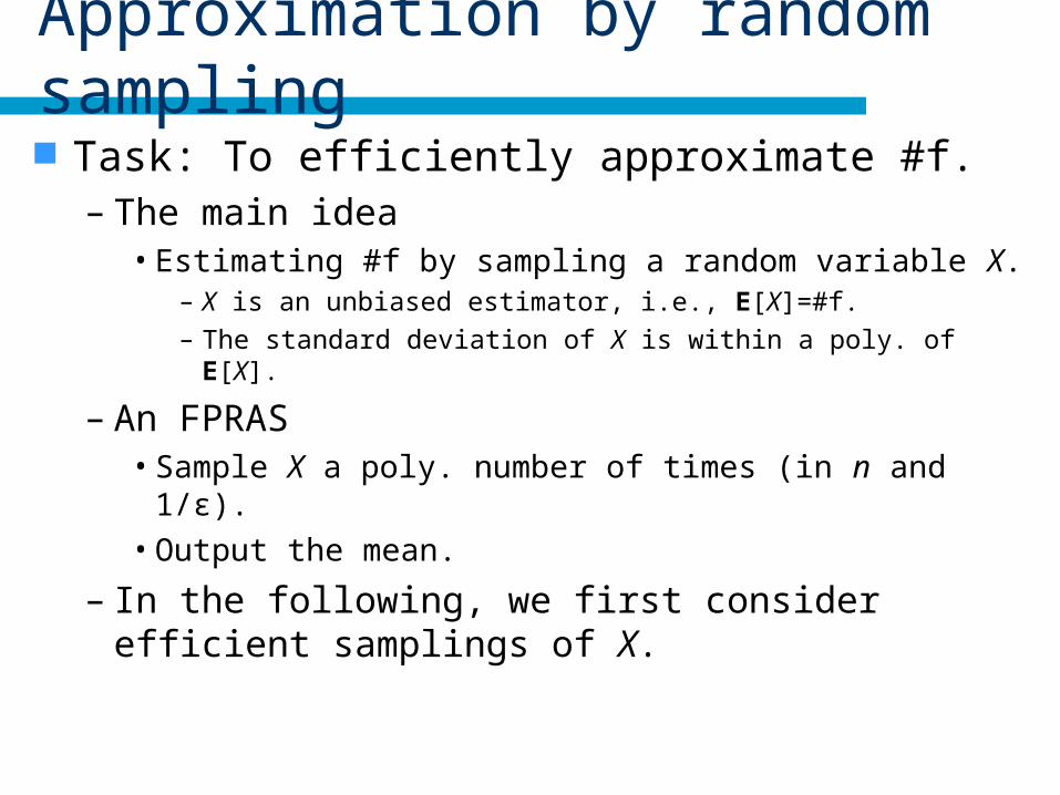
Approximation by random sampling

Task: To efficiently approximate #f.– The main idea

• Estimating #f by sampling a random variable X.– X is an unbiased estimator, i.e., E[X]=#f.

– The standard deviation of X is within a poly. of E[X].

– An FPRAS• Sample X a poly. number of times (in n and 1/ε).

• Output the mean.

– In the following, we first consider efficient samplings of X.

Constructing an unbiased estimator

Y and Y(τ) are defined as follows:– Y(τ): 2n (τ satisfies f), 0 (otherwise).– Pr(Y): uniform distribution on all 2n truth assignments.

E[Y(τ)] is then an unbiased estimator.

.#1

02

12

2

1

)()Pr()]([

satisfies :

satisfy not does : satisfies :

f

YYE

f

fn

n

fn

x1 x2 x3 f Y

0 0 0 1 8

0 0 1 1 8

0 1 0 1 8

0 1 1 1 8

x1 x2 x3 f Y

1 0 0 1 8

1 0 1 1 8

1 1 0 1 8

1 1 1 0 0

Standard deviation of Y(τ)

σ2(Y(τ)): variance– Square of the standard deviation.

.)(##2

#2

#2)(##22

2

#

#2

1)(##22

2

1

#02

1#2

2

1

)]([)()Pr()]([

2

2212

2

satisfy not does :

212

satisfies :

2

satisfy not does :

2

satisfies :

22

ff

ff

fff

fff

ff

YEYY

n

n

nnn

n

fn

nn

fn

fn

n

fn

Not bounded by a polynomial of n.Not useful for constructing an FPRAS.

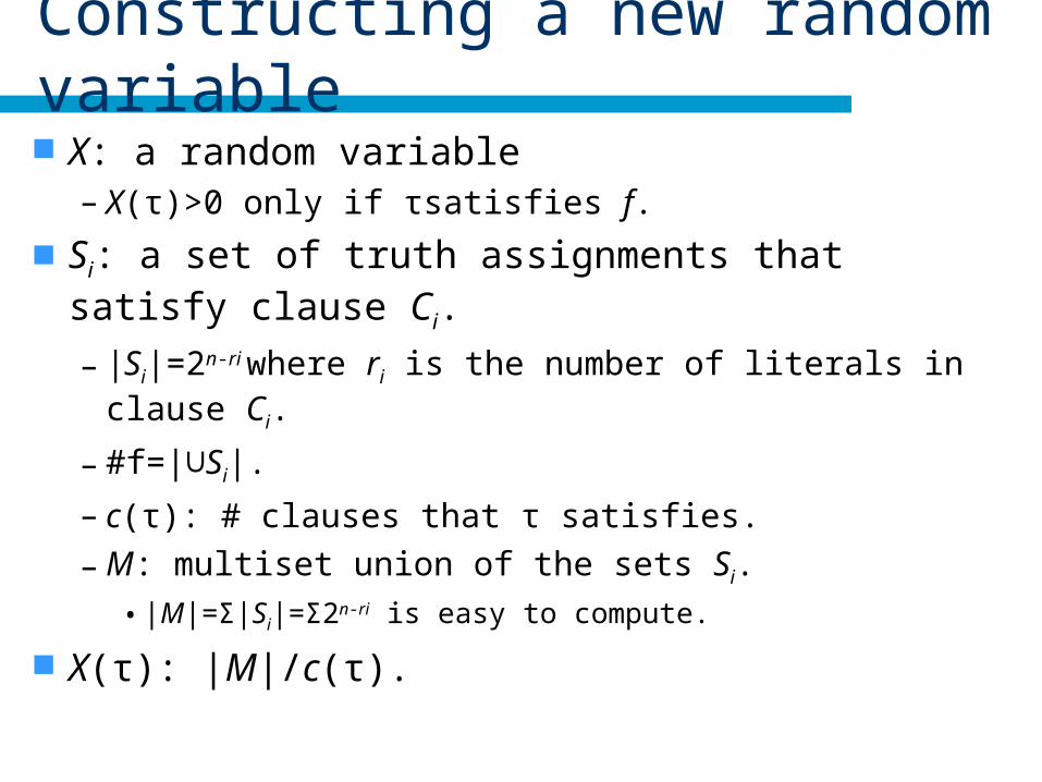
Constructing a new random variable

X: a random variable– X(τ)>0 only if τsatisfies f.

Si: a set of truth assignments that satisfy clause Ci.

– |Si|=2n-ri where ri is the number of literals in clause Ci.

– #f=|∪Si|.

– c(τ): # clauses that τ satisfies.

– M: multiset union of the sets Si.

• |M|=Σ|Si|=Σ2n-ri is easy to compute.

X(τ): |M|/c(τ).

Constructing a new random variable

Example:– fEX=(x1∧￢ x2) (∨ x2∧ ￢ x3 ) (∨ ￢ x1).

– Si: a set of truth assignments that satisfy clause Ci.

• S1={(1,0,0), (1,0,1)}, S2={(0,1,0), (1,1,0)}, S3={(0,0,0), (0,0,1), (0,1,0), (0,1,1)}, |S1 |=23-2=2, |S2|=23-2=2,|S3|=23-1=4.

• #f=|∪Si|, c(τ): # clauses that τ satisfies.

• M: multiset union of the sets Si.

– MEX=< (1,0,0), (1,0,1), (0,1,0), (1,1,0), (0,0,0), (0,0,1), (0,1,0), (0,1,1)>.

• X(τ)=|M|/c(τ).

x1 x2 x3 c X

0 0 0 0 8/1

0 0 1 0 8/1

0 1 0 2 8/2

0 1 1 1 8/1

x1 x2 x3 c X

1 0 0 1 8/1

1 0 1 1 8/1

1 1 0 1 8/1

1 1 1 0 0

An FPRAS Example

– fEX=(x1∧￢ x2) (∨ x2∧ ￢ x3 ) (∨ ￢ x1). for i=1 to k

– Pick one clause Cj from f with prob. |Sj|/|M|.• C1 with prob. 2/8.

– Pick a truth assignment τi satisfying Ci at random.• τi= (1,0,1).

– Find c(τi) and X(τi)= |M|/c(τi) .• c(τi)=1, X(τi)=8/1=8.

end-for output Xk=(X (τ1)+…+ X(τk))/k

– Xk=(8+4+8+8)/4=7.

x1 x2 x3 c X

0 0 0 0 8/1

0 0 1 0 8/1

0 1 0 2 8/2

0 1 1 1 8/1

x1 x2 x3 c X

1 0 0 1 8/1

1 0 1 1 8/1

1 1 0 1 8/1

1 1 1 0 0

From lemma 28.2,τ is picked with prob. c(τ)/|M|.

Overview

Lemma 28.5, Theorem 28.6There is an FPRAS for counting DNF solutions.

Lemma 28.2, 28.3X is an unbiased

estimator.

Lemma 28.4The variance of X issufficiently small.

Lemma 28.2

Random variable X can be efficiently sampled.– Sampling X is done with picking a random element

from the multiset M.• 1. pick a clause so that the probability of picking clause Ci

is | Si|/|M|.

• 2. among the truth assignments satisfying the picked clause, pick one at random.

– The probability with which truth assignment τ is picked is

.||

)(

||

1

||

||

satisfies : M

c

SM

S

i

i

Ci i

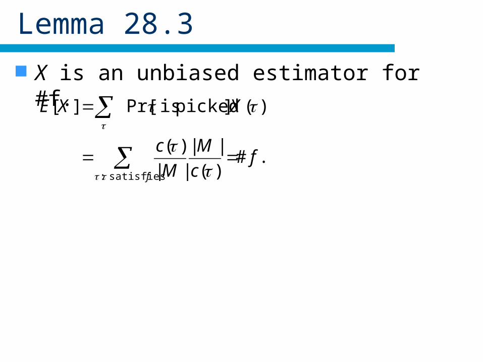
Lemma 28.3

X is an unbiased estimator for #f.

.#)(

||

||

)(

)(]picked is Pr[][

satisfies :

fc

M

M

c

XXE

f

Lemma 28.4

α=|M|/m. If m denotes the number of clauses in f, then

.1][

)(m

XE

X

.)(1 mc #clauses in f.

# clauses satisfied with τ

.||#][||

||1

1i

mi

m

ii

SfXEm

S

m

M

the average number oftruth assignments

satisfying one clause

the number of truthassignments satisfying

at least one clause

.)(

||)(

c

MX

.1

||)(

|| MX

m

M

.)( mX

.)1(|][)(| mXEX

].[)1(

)1()(

XEm

mX

Lemma 28.5 and Theorem 28.6

Let k=4(m － 1)2/ε2. For any ε>0, .

4

3]#|#Pr[| ffX k

Chebyshev’s inequality .)(

]|][Pr[|2

a

XaXEX

.4

1)1(

)1(2

1

][

)(11

][

)(

][

)(]][|][Pr[|

22

22

mmXE

X

k

XEk

X

XE

XXEXEX

kkkk

./)()(

],[][

kXX

XEXE

k

k

There is an FPRAS for the problemof counting DNF solutions.




Network reliability Input:

– a connected undirected graph G=(V, E), with failure prob. for each edge e.

• Parallel edges between two nodes are allowed.

Output:– The prob. that the graph

becomes disconnected.• Denote the prob. by

FAIL(p).

v1

v2v3

v4v5 v6

v7

v1

v2

v3

v4

v5

v6

v7

v1

v2

v3

v4

v5 v6

v7

disconnected still connected

Tractability of FAIL(p)

Tractable if FAIL(p) is not small.– “Small” means at least inverse polynomial.

– FAIL(p) can be estimated by sampling.• We will explain it later (in the proof of Theorem 28.11).

Intractable if FAIL(p) is small.– Sampling approaches do not work.

• Many samplings are required for the estimation.

– In the following, we assume that FAIL(p) ≦ n － 4. Pr(cut (C,C) gets disconnected)=pc.

– where c is the number of edges crossing the cut.

– pc decreases exponentially with capacity (# edges, c).

Ideas of the algorithm For any ε>0, we will show that only polynomially

many “small’’ cuts (in n and 1/ε) are responsible for 1 － ε fraction of the total failure probability FAIL(p). Moreover, these cuts, say E1,…,Ek, Ei ⊆E, can be enumerated in polynomial time.

We will construct a polynomial sized DNF formula f whose probability of being satisfied is precisely the probability that at least one of these cuts fails.

Illustration of the idea (1/2)

v1 v3

v4

v5

v6

v7

v1v3

v4

v5 v6

v7

v1v3

v4

v5 v6

v7

Prob. p2 p3 p5

Ratio of prob.1 － ε ε

Enumerable in polynomial time(Exercise 28.11-13)

Illustration of the idea (2/2)

e1

e2 e2

e3 e4

,211 ee xxD ,

432 eeek xxxD

cut E1 cut Ek

.1 kDDf

e1

e2

,3212 eee xxxD

cut E2

e3

One-to-onecorrespondence

xei is true with probability pei.

Lemma 28.8 (1/3)

The number of minimum cuts in G=(V,E) is bounded by n(n-1)/2.– Contractions of an edge.

v1v2

v7

v1 v3v1

v1

v7

v2,….,v6

{v1,….,v6} {v7}Cut ({v1,….,v6}, {v7}) survives.

Lemma 28.8 (2/3)

.)1(

2]survives ),Pr[(

nnCC

Let M be the number of minimum cuts in G.– M is bounded by n(n-1)/2 if

].survives ),Pr[(1),(

CCCC

.)1(

2]survives ),Pr[(1

cut minimum a is ),.(.:),(

nn

MCC

CCtsCC

.2

)1(M

nn

Lemma 28.8 (3/3)

H: a graph at the beginning of contraction process.– Contractions never decrease the capacity of the

minimum cut.• The degree of each node in H is at least c.

• m is the number of nodes in H.

• Hence, H must have at least cm/2 edges.

– The minimum cut survives with the probability (1-c/#edges).

.2

12/

1#

1

mcm

c

edges

c

.)1(

2

3

21

1

21

21]survives ),Pr[(

nnnnCC

Lemma 28.9 (1/3)

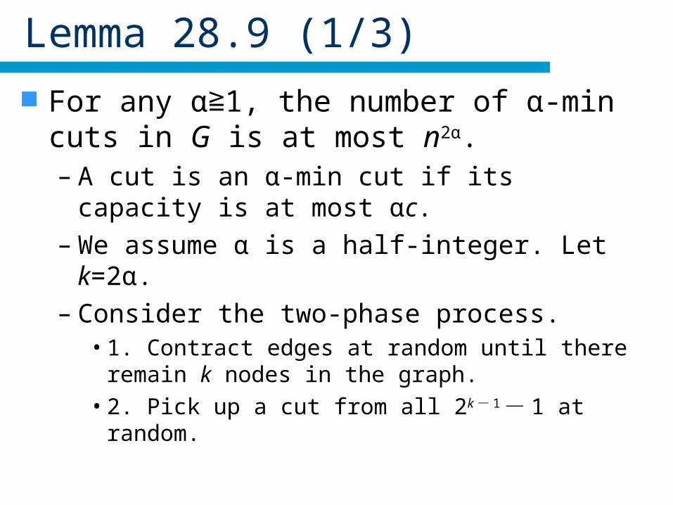
For any α 1, the number of α-min cuts in ≧ G is at most n2α.– A cut is an α-min cut if its capacity is at most αc.– We assume α is a half-integer. Let k=2α.– Consider the two-phase process.

• 1. Contract edges at random until there remain k nodes in the graph.

• 2. Pick up a cut from all 2k － 1 － 1 at random.

Lemma 28.9 (2/3)

Example– k=4.– Phase 1.

– Phase 2.

v1v2

v7

v1 v3v1

v1

v1

.)1()1(

1)1(

11

111

]survives ),Pr[(

knnn

kk

k

k

n

k

n

k

CC

11 2

1

12

1kk

10

41

9

41

7

41

Lemma 28.9 (3/3)

.11

1

1

)2(2

2

)1(2

1

2

2

1

)1()1(

1)1(

]phases twohe through tsurvives ),Pr[(

2

1

nn

knknn

k

n

k

knnn

kk

CC

k

k

FAIL(p)

In case that FAIL(p) ≦ n － 4. The failure probability of a minimum cut is pc ≦

FAIL(p) ≦ n － 4. pc = n － (2+δ). From lemma 28.9, for any α 1, the total failure ≧

probability of all cuts of capacity αc is at most pcαn2α = n － αδ.

Lemma 28.10 (1/3)

For any α,– – For bounding the total failure prob. of “large” capacity

cuts.– Number all cuts in G by increasing capacity.

• ck: the capacity of the k-th cut in this numbering.

• pk: the failure probability of the k-th cut.

• a: the number of the first cut of capacity greater than αc.

– It suffices to show that

.2

1]fails capacity ofcut somePr[

ncZ

.2

, 2

12

2

2

2

npnpnpppZnak

k

na

akk

nakk

na

akk

akk

Lemma 28.10 (2/3)

Illustration of the idea of lemma 28.10– Number all cuts in G by increasing capacity.

.:sum 1nS .

2:sum 2

nS

.2

1

nZ

.1 cc .1 cca .cca .2 ccna

.12 cc

na

Lemma 28.10 (3/3)

For ck (a≦k≦a+n2α),

– ck>αc → pk<pαc = n － α(2+δ) .

For ck (k≧a+n2α),

– at most n2α cuts with the capacity less than αc exist.– from lemma 28.9.

• Then, for any β, cn2β β≧ c.

• Replacing n2βby k, we obtain β=log k/(2 log n), and

• Therefore,

.)2(2)2(

22

nnnnpna

ak

na

akk

.2

2/1

1

222

)2/1(

nndkkppnnk

knak

k

.)( )2/1(ln2

ln kpp n

kc

k

Theorem 28.11 (1/4)

There is an FPRAS for estimating network reliability.– In case that FAIL(p)>n － 4.– The network is connected/disconnected: binomial

distribution.• Sampling and Chernoff bound are used to estimate

FAIL(p)=μ.

.])1(Pr[,])1(Pr[

,/log12)/(log12

.])1(Pr[,])1(Pr[

43/log1262/log12

242

3/2/ 22

neXneX

nnnk

eXeX

nn

kk

)1( )1(

4/1 n6/1 n The light blue areas areless than 1/4 if n>2.

Theorem 28.11 (2/4)

In case that FAIL(p)≦n － 4. α must be determined for enumerating graphs

with high probabilities such that

.)(FAIL 2

1]fails capacity ofcut somePr[ )2(

npnc

This inequality is given in the textbook,but this seems to contradict with

)(FAIL)2( ppn c in p. 300.

total failureone failure

By lemma 28.10

.log2

2/log2

log

2/log21

?

)2(

nn

nn

Theorem 28.11 (3/4)

By lemma 28.9, Pr[one of the first n2α fails] (1≧ － ε)FAIL(p). The first n2α =O(n4/ε) cuts are enumerable in

polynomial time (Exercise 28.11-13).

.2 ccn

p2 p3 p5

1 － ε ε

,211 ee xxD .21 n

DDf .321

2 eeenxxxD

Theorem 28.11 (4/4)

To reduce the case of arbitrary edge failure probabilities, parallel edges are used.

failureprobability

pe

parallel –(ln pe)/θ edges

failureprobability θ

all edges are disconnectedwith prob.

/)(ln)1( ep

.)1(lim ln/)(ln0 e

pp pe ee

Documents

Approximation Algorithms Chapter 28: Counting Problems 2003/06/17