Embed Size (px)
Citation preview
Approximation Algorithms for Perishable
Inventory Systems with Setup Costs
Huanan Zhang, Cong Shi, Xiuli ChaoIndustrial and Operations Engineering, University of Michigan, MI 48105, zhanghn, shicong, [email protected]
We develop the first approximation algorithm for periodic-review perishable inventory systems with setup
costs. The ordering lead time is zero. The model allows for correlated demand processes which generalize the
well-known approaches to model dynamic demand forecast updates. The structure of optimal policies for this
fundamental class of problems is not known in the literature. Thus, finding provably near-optimal control
policies has been an open challenge. We develop a randomized proportional-balancing policy (RPB) that can
be efficiently implemented in an online manner, and show that it admits a worst-case performance guarantee
between 3 and 4. The main challenge in our analysis is to compare the setup costs between RPB and the
optimal policy in the presence of inventory perishability, which departs significantly from the previous works
of Chao et al. (2015b,a). The numerical results show that the average performance of RPB is good (within
1% of optimality under i.i.d. demands and within 7% under correlated demands).
Key words : inventory, perishable products, setup costs, randomized algorithms, worst-case analysis
Received October 2014; revisions received March 2015, October 2015, December 2015; accepted January
2016.
1. Introduction
We study the periodic-review perishable inventory systems with setup costs under a general class of
associated demand processes (see §2). Undoubtedly, perishable products are an indispensable part
of our lives. For example, perishable products such as meat, fruit, vegetable, dairy products, and
frozen foods constitute the majority of supermarket sales. Moreover, virtually all pharmaceuticals
belong to the category of perishable products. Blood bank provides another salient example where
whole blood has finite lifetimes (see, e.g., Prastacos (1984)). In general, the analysis of perishable
products is much harder than that of non-perishables.
The work on classical perishable inventory systems dates back to Nahmias (1975) and Fries
(1975) who characterized the structure of the optimal ordering policy with i.i.d. demands and
no setup costs for backlogging and lost-sales models, respectively. We refer interested readers to
Karaesmen et al. (2011) and Chao et al. (2015b,a) for a review of the field. Unfortunately, almost
all the papers in the existing perishable inventory literature do not model positive setup costs
1
Zhang, Shi and Chao: Approximation Algorithms for Perishable Inventory Systems with Setup Costs 2
(mainly due to its mathematical intractability), despite the fact that fixed cost is often unavoidable
in many practical settings. As a result, little is known about the structure of the optimal policies
for this class of problems with setup costs. Thus, finding provably near-optimal control policies has
been an open challenge. In this paper, we propose an efficient randomized proportional-balancing
policy that admits a worst-case performance guarantee between 3 and 4. We also demonstrate via
numerical experiments that the proposed policy performs consistently well.
Relevant literature. Nahmias (1978) was the first to analyze perishable inventory problems
with positive setup costs. He showed that the cost function is in general not K-convex and that
(s,S) policy may not be optimal. Indeed, the optimal control policy for this class of problems is very
complicated, and there is no known structural characterization for it. Nevertheless, Nahmias (1978)
demonstrated, computationally, that (s,S) type policies perform well under i.i.d. demands. Lian
and Liu (1999) also considered a periodic-review model with positive setup costs, and constructed
a multi-dimensional Markov chain to model and analyze the inventory-level process. Lian et al.
(2005) used the same costs and replenishment assumptions as Lian and Liu (1999), and constructed
a multi-dimensional Markov chain to model the inventory-level process to derive cost expressions.
They numerically showed that the variability in the lifetime distribution can have a significant
effect on system performance. However, the aforementioned heuristic policies can only be applied
to i.i.d. demand processes, and furthermore they lack any performance guarantees.
Main results and contribution. The contribution of this note is to present the first approx-
imation algorithm for periodic-review perishable inventory system with setup costs that admits
a worst-case performance guarantee between 3 and 4. The result holds not only for independent
demand processes, but also for a general class of correlated processes, which we call associated
demand processes. The proposed policy will be referred to as a randomized proportional-balancing
policy (RPB). As seen from our literature review, this class of problems is fundamental in perish-
able inventory literature that has challenged researchers for decades; yet little is known about both
the structure of optimal policies and the design of provably-good heuristic policies.
Our approach builds on Chao et al. (2015b,a) on perishable inventory systems without setup
costs. In particular, we adopt their marginal cost accounting schemes of computing marginal hold-
ing, backlogging and outdating costs. The main idea underlying this marginal cost accounting
approach is to decompose the total cost in terms of the marginal costs of individual decisions (rather
than the conventional per-period cost accounting). However, the nonlinear setup costs make the
balancing of the various costs much more complicated. Thus, we construct a randomized algorithm
to tackle this problem, striking a right balance between different cost components. The worst-case
performance analysis is inevitably much more sophisticated, due to inventory perishability. The key
Zhang, Shi and Chao: Approximation Algorithms for Perishable Inventory Systems with Setup Costs 3
technical challenge is to amortize the setup costs of RPB against the optimal policy. We note that
Levi and Shi (2013) on stochastic lot-sizing problems had the same challenge but their partition
of periods is rather straightforward without perishability, while our problem needs to consider the
inventory age information that is essential in the analysis of our system. (To this end, we also
provide a detailed discussion in §4 on why the previous partition in Levi and Shi (2013) fails to
work in our perishable inventory systems.) This additional information on inventory age enables
us to amortize the setup cost incurred by RPB against that of the optimal policy. On the technical
level, we provide a novel sample-path argument that shows that the optimal policy has to place an
order between two consecutive problematic periods in which the relationship between the trimmed
ending inventory levels of RPB and the optimal policy is unclear (due to randomized decisions).
This is in sharp contrast with the averaging argument used in Levi and Shi (2013). Moreover, Levi
and Shi (2013) need not consider the age information in their analysis. Our construction provides
the right and delicate framework to use the age information to analyze the system, which could
be useful in analyzing other more complex perishable inventory systems (e.g., with positive lead
times and/or finite ordering capacities).
We also demonstrate through an extensive computational study that our proposed algorithm
performs quite well empirically (with average error under 7% and maximum error of 11.28% under
correlated demands). Our algorithm has also comparable (if not, better) performance with that of
Nahmias (1978) under i.i.d. demands, in which both algorithms perform very close to optimal.
Structure and general notation. The rest of this paper is organized as follows. In §2, we
formally describe the periodic-review perishable inventory systems with setup costs. In §3, we
introduce the randomized proportional-balancing policy (RPB). In §4, we carry out a worst-case
performance analysis of RPB. In §5, we demonstrate the empirical performance of RPB.
Throughout this paper, we often distinguish between a random variable and its realizations using
capital and lower-case letters, respectively. For any real numbers x and y, we denote x+ = maxx,0,
x∨ y = maxx, y, and x∧ y = minx, y. In addition, for a sequence x1, x2, . . . and any integers t
and s with t≤ s, we denote x[t,s] =∑s
j=t xj and x[t,s) =∑s−1
j=t xj. The indicator function 1(A) takes
value 1 if A is true and 0 otherwise, and “, ” stands for “defined as”.
2. Perishable Inventory Systems with Setup Costs
We formally describe the stochastic periodic-review perishable inventory system with setup costs
over a planning horizon T (possibly infinite), indexed by t= 1, . . . , T . The product lifetime is m≥ 2,
i.e., items perish after staying in inventory for m periods if not consumed. The ordering lead time
is 0 (see, e.g., Karaesmen et al. (2011)).
Zhang, Shi and Chao: Approximation Algorithms for Perishable Inventory Systems with Setup Costs 4
Cost structure. The unit holding and shortage costs are denoted by h and b, respectively, and
the unit outdating cost is θ. Without loss of generality, we assume the unit purchasing cost c= 0
(see a detailed cost transformation in Chao et al. (2015b)). In addition, there is a setup cost K
that is incurred whenever an order is placed. The discount factor is α∈ [0,1] (but α is strictly less
than 1 if T =∞), and the firm’s objective is to minimize the expected total discounted cost. (Our
model and results can allow for non-stationary setup costs Kt as long as they satisfy αKt+1 ≤Kt.)
Demand structure. We adopt the same demand structure as that of Chao et al. (2015a), where
the demands D1, . . . ,DT are associated (which is defined formally below). At the beginning of each
period t, the manager observes an information set denoted by Ft. The information set Ft contains
the past information accumulated up to the beginning of period t, including the realized demands
d1, . . . , dt−1 in the first t− 1 periods and possibly some other exogenous information (e.g., state of
economy, weather, etc). The information set Ft | t ∈ [1, T ] form the filtration over a probability
space (Ω,F , P ). We assume that the conditional expectations of all relevant quantities, given Ft,
are well-defined. The formal definition of associated demand process is as follows.
Definition 1 (Chao et al. (2015a)). A stochastic demand process Dt; t= 1,2, . . . with fil-
tration Ft, t ≥ 1 is called associated if, conditional on Ft, the random demand vector Dt =
(Dt,Dt+1, . . . ,DT ) satisfies E[f(Dt)g(Dt)] ≥ E[f(Dt)] E[g(Dt)] for all non-decreasing (or non-
increasing) functions f and g for which the expectations E[f(Dt)], E[g(Dt)], E[f(Dt)g(Dt)] exist.
The class of associated processes includes not only independent demand processes, but also
most time-series demand models such as autoregressive (AR) and autoregressive moving aver-
age (ARMA) demand models (Box et al. (2008)), multiplicative auto-regression model (Levi
et al. (2008)), demand forecast updating models such as martingale models for forecast evolution
(MMFE) (Heath and Jackson (1994)), demand processes with advance demand information (ADI)
(Gallego and Ozer (2001)), as well as economic-state driven demand processes such as Markov
modulated demand processes with stochastically monotone transition matrix, among others. We
refer interested readers to Chao et al. (2015a) for more discussions.
System dynamics. In perishable inventory systems, any inventory unit that stays in the system
for m periods without meeting the demand expires and exits the system. Thus, we use a vector to
keep track of the inventory age information, which results in a multidimensional state space.
At the beginning of each period t, t= 1,2, . . . , T , we are endowed with the realized information ft.
(Here we abuse the notation to use ft to denote the realized information up to time t, which should
be distinguished with the filtration Ft.) The starting inventory at period t is xt = (xt,1, . . . , xt,m−1),
where for i = 1, . . . ,m − 2, xt,i is the inventory level of product whose remaining lifetime is i
periods, and xt,m−1 is the number of product whose remaining lifetime is m− 1 minus the number
Zhang, Shi and Chao: Approximation Algorithms for Perishable Inventory Systems with Setup Costs 5
of backlogs. After receiving the order qt in period t, the random demand Dt will be realized
(denote its realization by dt) and satisfied to the maximum extent by FIFO issuing policy, i.e., the
oldest inventory meets demand first. Following the convention by Nahmias (1975), we assume the
inventory units that will perish at the end of this period also incur a holding cost. The discounted
one-period cost is αt−1(K ·1(qt > 0) +h(yt− dt)+ + b(dt− yt)+ + θet
), where yt =
∑m−1
i=1 xt,i + qt is
the total inventory level (after ordering) in period t, and et = (xt,1−dt)+ is the outdating inventory.
Then, the system proceeds to period t+ 1 with xt+1 given by
xt+1,j =
xt,j+1−
(dt−
j∑i=1
xt,i
)++
, for 1≤ j ≤m− 2, (1)
xt+1,m−1 = qt−
(dt−
m−1∑i=1
xt,i
)+
. (2)
For simplicity we assume that the system is initially empty. Then the total expected discounted
cost for any given FIFO issuance policy P can be written as
C (P ) =E
[T∑t=1
αt−1(K ·1(Qt > 0) +h(Yt−Dt)
+ + b(Dt−Yt)+ + θEt
)]. (3)
Note that, the quantities Qt, Yt,Et and Xt depend on the policy P, and we shall make the depen-
dency explicit whenever necessary, i.e., writing them as QPt , Y
Pt ,E
Pt and XP
t .
3. Randomized Proportional-Balancing Policy
We present the randomized proportional-balancing policy (denoted by RPB) and its worst-case
performance guarantee. We start by reviewing the nested marginal holding and outdating cost
accounting scheme used in Chao et al. (2015b,a). The main idea is to decompose the total cost in
terms of the marginal costs of individual decisions (first used in Levi et al. (2007)). That is, we
associate the decision in period t with its affiliated cost contributions to the system. These costs
are only affected by future demands but not by future decisions. These marginal costs may include
costs (associated with the decision) incurred in both the current and subsequent periods.
3.1. Review of the marginal cost accounting scheme
Under FIFO issuing policy, after a unit is ordered, the number of periods that it stays in the system
is not affected by future decisions but only affected by future demands. In other words, the total
expected holding and outdating cost of any unit is determined in the period in which that unit is
ordered.
Zhang, Shi and Chao: Approximation Algorithms for Perishable Inventory Systems with Setup Costs 6
Marginal holding and outdating costs. Suppose an order quantity qPt ≥ 0 is placed by a
policy P in period t. Then the total expected marginal holding and outdating cost of those qPt units
can be computed via a recursive equation. For t≤ s < t+m, let B[t,s)(xPt ) denote the total number
of outdated units from period t up to period s− 1 when the starting inventory at the beginning of
period t is xPt . With the convention that B[t,t)(xPt )≡ 0, we can write B[t,s)(x
Pt ) recursively by
B[t,s)(xPt ) = max
s−t∑j=1
xPt,j −D[t,s), B[t,s−1)(xPt )
, t < s≤ t+m− 1. (4)
Using B[t,s)(xPt ), the nested marginal holding cost HP
t can be written as, for 1≤ t≤ T ,
HPt =HP
t (qPt ;xPt ), h(t+m−1)∧T∑
s=t
αs−1(qPt −
(D[t,s] +B[t,s)(x
Pt )−
m−1∑j=1
xPt,j)+)+
, (5)
and the nested marginal outdating cost ΘPt can be written as, for 1≤ t≤ T −m+ 1,
ΘPt = ΘP
t (qPt ;xPt ), αt+m−2θEt+m−1 = αt+m−2θ(qPt +
m−1∑j=1
xPt,j −B[t,t+m−1)(xPt )−D[t,t+m−1]
)+
, (6)
and ΘPt ≡ 0 for t= T −m+2, . . . , T as the ordered units do not expire within the planning horizon.
It is clear that both HPt (·) and ΘP
t (·) are increasing in qPt .
Backlogging cost and setup cost. It is clear that in period t, no future marginal backlogging
cost is caused by the current order qPt , since any under-ordering can be corrected by subsequent
orders. As a result, the marginal backlogging cost in period t is the same as the conventional
backlogging cost in period t, which can be written as
ΠPt = ΠP
t (qPt ;xPt ), αt−1 b(Dt−
m−1∑i=1
xPt,i− qPt)+
. (7)
Moreover, the setup cost in any period t is also only affected by qPt , which is αt−1K ·1(qPt > 0).
System total cost. Since the system is initially empty, the expected total system cost C (P )
of policy P can be obtained by summing (5), (6), (7) and the setup costs over t from 1 to T , and
then taking expectations. Thus, (3) can be rewritten as
C (P ) = E
[T∑t=1
(HPt (qPt ;xPt ) + ΠP
t (qPt ;xPt ) + ΘPt (qPt ;xPt ) +αt−1K ·1(qPt > 0)
)], (8)
and the system dynamics are governed by (1) and (2).
Zhang, Shi and Chao: Approximation Algorithms for Perishable Inventory Systems with Setup Costs 7
3.2. RPB policy
To describe the randomized proportional-balancing (RPB) policy, we modify the definition of the
information set ft to also include the implemented decisions of the randomized policy up to period
t− 1. To determine whether or not to place an order, and how much to order, in period t, RPB
computes the following quantities:
(a) Compute qt that balances the conditional expected marginal holding and outdating costs of
these units against the conditional expected backlogging cost in period t. That is, qt solves
mh+θ2(m−1)h+θ
E[HRPBt (qt) + ΘRPB
t (qt) | ft]
=E[ΠRPBt (qt) | ft
], θt, (9)
where qt is referred to as the proportional balancing quantity, and θt the proportional balancing
cost. The solution to (9) is unique and can be computed efficiently via bisection search.
(b) Compute the (proportional) balancing-K-quantity qt that solves
mh+θ2(m−1)h+θ
E[HRPBt (qt) + ΘRPB
t (qt) | ft]
=K.
That is, ordering qt that balances a proportion of the marginal holding and outdating costs
with setup cost K.
(c) Compute E[ΠRPBt (qt) | ft], i.e., the conditional expected backlogging cost in period t if one
orders the balancing-K-quantity qt in period t.
(d) Compute E[ΠRPBt (0) | ft], i.e., the conditional expected backlogging cost in period t resulting
from not ordering in period t.
Description of RPB policy. Let Pt denote the probability that RPB policy places an order
in period t which is a-priori random, and let pt = (Pt | ft). Given ft, the RPB policy determines
the ordering decisions according to two cases below:
Case (I). If the proportional balancing cost exceeds K, i.e., θt ≥K, then the RPB policy orders
the balancing quantity qRPBt = qt in period t with probability pt = 1.
Case (II). If the proportional balancing cost is less than K, i.e., θt <K, then the RPB policy
orders the balancing-K-quantity (i.e., qRPBt = qt) in period t with probability pt and orders nothing
with probability 1− pt, where the probability pt is computed by solving equation
ptK = pt ·E[ΠRPBt (qt) | ft] + (1− pt) ·E[ΠRPB
t (0) | ft]. (10)
This completes the description of the RPB policy. We offer some intuitive explanations as follows.
In Case (I), that is when θt ≥K, the fixed ordering cost K is not dominant compared to the other
Zhang, Shi and Chao: Approximation Algorithms for Perishable Inventory Systems with Setup Costs 8
cost components, hence the policy only strives to achieve (the right) balance between marginal
holding, outdating, and shortage costs. In Case (II), the underlying reasoning behind the choice of
the particular randomization in (10) is that, the policy attempts to balance between the three cost
components, namely, holding and outdating cost, backlogging cost and setup cost associated with
period t. In particular, since we order the balancing-K-quantity with probability pt and do not
order anything with probability 1−pt, the conditional expected proportional holding and outdating
cost for this case is
mh+θ2(m−1)h+θ
E[HRPBt (qRPBt ) + ΘRPB
t (qRPBt ) | ft] (11)
= mh+θ2(m−1)h+θ
ptE[HRPB
t (qt) + ΘRPBt (qt) | ft] + (1− pt)E[HRPB
t (0) + ΘRPBt (0) | ft]
= ptK.
By the selection of pt in (10), the conditional expected backlogging cost is
E[ΠRPBt (qRPBt ) | ft] = ptE[ΠRPB
t (qt) | ft] + (1− pt)E[ΠRPBt (0) | ft] = ptK. (12)
Since pt is the ordering probability in Case (II), the expected fixed ordering cost is also ptK.
It can be shown the pt that solves (10) is
0≤ pt =E[ΠRPB
t (0) | ft]K −E[ΠRPB
t (qt) | ft] +E[ΠRPBt (0) | ft]
< 1, (13)
where the above inequalities follow from the fact that θt < K and qt > qt, which implies that
E[ΠRPBt (qt) | ft]<E[ΠRPB
t (qt) | ft] = θt <K. We remark that when the setup cost K = 0, the RPB
policy reduces exactly to the PB policy proposed in Chao et al. (2015b), i.e., RPB is a generalization
of PB in the presence of setup costs.
The following is the main theoretical result of this paper.
Theorem 1. When the demand process is associated, the RPB policy for perishable inventory
system with setup cost and m≥ 2 periods of product lifetime has a worst-case performance guarantee
of(
3 + (m−2)h
mh+θ
), i.e., for any instance of the problem, the expected cost of the RPB policy is at
most(
3 + (m−2)h
mh+θ
)times the expected cost of an optimal policy.
The balancing ratio on the left hand side of (9) is chosen such that the resulting RPB policy
admits the tightest worst-case performance guarantee. Suppose an arbitrary balancing ratio β ∈
(0,1] is used to construct RPB. Then one can show that it admits a worst-case performance
guarantee of (2β+ 1)/minβ,β0, where β0 = mh+θ2(m−1)h+θ
(which is obtained from (22) in our worst-
case analysis). This worst-case performance guarantee is minimized when β = β0.
Zhang, Shi and Chao: Approximation Algorithms for Perishable Inventory Systems with Setup Costs 9
Remark on discrete demand and order quantities: If the demand and order quantities are
discrete, then we can always write qt = λtq1t + (1− λt)q2
t , where q1t and q2
t = q1t + 1 are consecutive
integers with q1t ≤ qt < q2
t and 0< λt ≤ 1. Similarly, we write qt = λtq1t + (1− λt)q2
t , where q1t and
q2t = q1
t + 1 are consecutive integers with q1t ≤ qt < q2
t and 0< λt ≤ 1. In Case (I), RPB orders either
q1t units (with probability λt) or q2
t units (with probability 1− λt). In Case (II), RPB orders either q1t
units (with probability ptλt), or q2t units (with probability pt(1− λt)), or zero unit (with probability
1− pt). This randomized procedure will not affect our worst-case performance guarantee, and we
refer readers to the detailed discussions in §4.3 of Levi et al. (2007) and also §6 of Shi et al. (2014).
4. Worst-Case Performance Analysis
We carry out a worst-case performance analysis of RPB policy. For simplicity, we provide the proofs
with a discount factor α= 1 (albeit the analysis holds under general α∈ [0,1]).
We first describe a concept called “trimmed inventory level” (see Chao et al. (2015a)). The
trimmed inventory level, denoted by Yt,s for any s ≥ t ≥ 1, is defined as the inventory at the
beginning of period s for the products that are ordered in period t or earlier. Equivalently, Yt,s is
the inventory level Ys (after ordering) at the beginning of period s less the total order quantity in
periods t+ 1, . . . , s, i.e., Yt,s = Ys−∑s
s′=t+1Qs′ . By definition, Yt,t = Yt and we also have
Yt,s = Yt,s′ −D[s′,s)−E[s′,s), t≤ s′ < s≤ t+m− 1, (14)
Yt,s = Yt,t+m−1−D[t+m−1,s), s > t+m− 1. (15)
Note that Yt,s can be negative when s is large enough. These trimmed inventory levels serve as a
generalization of the traditional inventory levels, as they provide critical partial information on the
age of the on-hand products. Due to the nature of perishable systems, it is impossible to quantify
the effect of the decision made in the current period t on future costs only through the traditional
total inventory level Yt. The trimmed inventory levels provide a tractable way to analyze this effect,
and also provide the right framework for coupling the marginal holding, outdating and setup costs
in different systems. Furthermore, for any realization ft, if pt < 1, then we denote RPB as the
policy that orders exactly the same as RPB before period t, but orders qt at t (instead of using a
randomized decision between 0 and qt), and orders 0 afterwards.
We now compare the costs of RPB policy against that of an optimal policy, denoted by OPT.
For each realization fT , we partition all the periods into the following sets:
T1H =t : pt = 1 and yOPTt > yRPBt
; (16)
T1Π =t : pt = 1 and yOPTt ≤ yRPBt
; (17)
Zhang, Shi and Chao: Approximation Algorithms for Perishable Inventory Systems with Setup Costs 10
T2Π =t : pt < 1 and xRPBt ≥ yOPTt
; (18)
T2H =t : pt < 1 and xRPBt < yOPTt and ∃s∈ [t, (t+m− 1)∧T ], yOPTt,s > yRPBt,s
; (19)
T2M =t : pt < 1 and xRPBt < yOPTt and ∀s∈ [t, (t+m− 1)∧T ], yOPTt,s ≤ yRPBt,s
. (20)
Lemma 1 shows that the backlogging cost of OPT can cover that of RPB within set T1Π
⋃T2Π,
which is formally stated below. We relegate its detailed proof to the electronic companion.
Lemma 1. For each sample path fT , we have
T∑t=1
ΠOPTt ≥
T∑t=1
[ΠRPBt ·1
(t∈T1Π
⋃T2Π
)]. (21)
Lemma 2 shows how to amortize the sum of marginal holding and outdating costs against that
of OPT, which follows identical arguments used in Chao et al. (2015a); hence its proof is omitted.
Lemma 2. For each sample path fT , we have
T∑t=1
(HOPTt + ΘOPT
t
)≥ mh+ θ
2(m− 1)h+ θ
T∑t=1
[(HRPB
t + ΘRPBt ) ·1
(t∈T1H
⋃T2H
)]. (22)
The next result is a key lemma for this paper. It suggests that the total setup cost incurred by
OPT can cover the total setup cost incurred by RPB for periods within the set T2M . Note that
T2M is the most “problematic” set of periods because we are unsure whether the trimmed ending
inventory levels of RPB are higher or lower than those of OPT due to randomized decisions.
Lemma 3. For each sample path fT , the following inequality holds for the OPT and RPB policies,
T∑t=1
1(qOPTt > 0)≥T∑t=1
1(qRPBt > 0 and t∈T2M). (23)
Proof. For a fixed sample path fT , each period t deterministically belongs to one of the sets in
T1H , T1Π, T2Π, T2H and T2M . Denote all the periods in T2M with positive ordering quantities by
t∈T2M : qRPBt > 0
= t1, t2, . . . , tn.
See Figure 1 for an illustration of all such periods.
If this set is empty, i.e., n= 0, then (23) trivially holds. Otherwise, it follows from the definition
of t1, t2, . . . , tn that the right hand side of (23) is equal to n. Thus, it suffices to prove that OPT
places at least n orders. We first show that,
t1∑t=1
1(qOPTt > 0)≥ 1. (24)
Zhang, Shi and Chao: Approximation Algorithms for Perishable Inventory Systems with Setup Costs 11
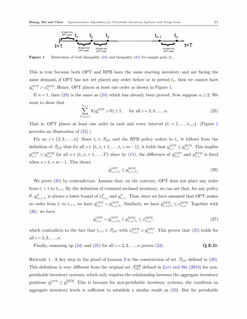
Figure 1 Illustration of both Inequality (24) and Inequality (25) for sample path fT .
This is true because both OPT and RPB have the same starting inventory and are facing the
same demand, if OPT has not yet placed any order before or in period t1, then we cannot have
yOPTt1>xRPBt1
. Hence, OPT places at least one order as shown in Figure 1.
If n= 1, then (23) is the same as (24) which has already been proved. Now suppose n≥ 2. We
want to show thatti+1∑t=ti+1
1(qOPTt > 0)≥ 1, for all i= 2,3, . . . , n. (25)
That is, OPT places at least one order in each and every interval ti + 1, . . . , ti+1. (Figure 1
provides an illustration of (25).)
Fix an i ∈ 2,3, . . . , n. Since ti ∈ T2M and the RPB policy orders in ti, it follows from the
definition of T2M that for all s∈ ti, ti + 1, . . . , ti +m−1, it holds that yOPTti,s≤ yRPBti,s
. This implies
yOPTti,s≤ yRPBti,s
for all s ∈ ti, ti + 1, . . . , T since by (15), the difference of yOPTti,sand yRPBti,s
is fixed
when s > ti +m− 1. This shows
yOPTti+1,ti≤ yRPBti+1,ti
. (26)
We prove (25) by contradiction. Assume that, on the contrary, OPT does not place any order
from ti + 1 to ti+1. By the definition of trimmed on-hand inventory, we can see that, for any policy
P, yPti+1,tiis always a lower bound of xPti+1
and yPti+1. Thus, since we have assumed that OPT makes
no order from ti to ti+1, we have yOPTti+1= yOPTti+1,ti
. Similarly, we have yRPBti+1,ti≤ xRPBti+1
. Together with
(26), we have
yOPTti+1= yOPTti+1,ti
≤ yRPBti+1,ti≤ xRPBti+1
, (27)
which contradicts to the fact that ti+1 ∈T2M with xRPBti+1< yOPTti+1
. This proves that (25) holds for
all i= 2,3, . . . , n.
Finally, summing up (24) and (25) for all i= 2,3, . . . , n proves (23). Q.E.D.
Remark 1. A key step in the proof of Lemma 3 is the construction of set T2M defined in (20).
This definition is very different from the original set T LS2M defined in Levi and Shi (2013) for non-
perishable inventory systems, which only requires the relationship between the aggregate inventory
positions yOPTt ≤ yRPBt . This is because for non-perishable inventory systems, the condition on
aggregate inventory levels is sufficient to establish a similar result as (23). But for perishable
Zhang, Shi and Chao: Approximation Algorithms for Perishable Inventory Systems with Setup Costs 12
OPT RPB
t
Dt=2
t+1
OPT
ordered at t-1
ordered at t
OPT
OOPTt=1
O t=3
RPB RPB
RPB
_ __
_
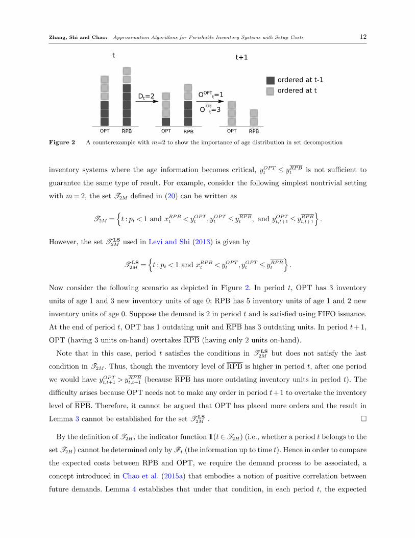
Figure 2 A counterexample with m=2 to show the importance of age distribution in set decomposition
inventory systems where the age information becomes critical, yOPTt ≤ yRPBt is not sufficient to
guarantee the same type of result. For example, consider the following simplest nontrivial setting
with m= 2, the set T2M defined in (20) can be written as
T2M =t : pt < 1 and xRPBt < yOPTt , yOPTt ≤ yRPBt , and yOPTt,t+1 ≤ yRPBt,t+1
.
However, the set T LS2M used in Levi and Shi (2013) is given by
T LS2M =
t : pt < 1 and xRPBt < yOPTt , yOPTt ≤ yRPBt
.
Now consider the following scenario as depicted in Figure 2. In period t, OPT has 3 inventory
units of age 1 and 3 new inventory units of age 0; RPB has 5 inventory units of age 1 and 2 new
inventory units of age 0. Suppose the demand is 2 in period t and is satisfied using FIFO issuance.
At the end of period t, OPT has 1 outdating unit and RPB has 3 outdating units. In period t+ 1,
OPT (having 3 units on-hand) overtakes RPB (having only 2 units on-hand).
Note that in this case, period t satisfies the conditions in T LS2M but does not satisfy the last
condition in T2M . Thus, though the inventory level of RPB is higher in period t, after one period
we would have yOPTt,t+1 > yRPBt,t+1 (because RPB has more outdating inventory units in period t). The
difficulty arises because OPT needs not to make any order in period t+1 to overtake the inventory
level of RPB. Therefore, it cannot be argued that OPT has placed more orders and the result in
Lemma 3 cannot be established for the set T LS2M .
By the definition of T2H , the indicator function 1(t∈T2H) (i.e., whether a period t belongs to the
set T2H) cannot be determined only by Ft (the information up to time t). Hence in order to compare
the expected costs between RPB and OPT, we require the demand process to be associated, a
concept introduced in Chao et al. (2015a) that embodies a notion of positive correlation between
future demands. Lemma 4 establishes that under that condition, in each period t, the expected
Zhang, Shi and Chao: Approximation Algorithms for Perishable Inventory Systems with Setup Costs 13
marginal holding and outdating costs with known information 1(t ∈T1H
⋃T2H) is in fact greater
than or equal to those without knowing the information.
Lemma 4. If the demand process D1, . . . ,DT is associated, then for each period t= 1, . . . , T ,
E[1(t∈T1H
⋃T2H
)|Ft
]·E[HRPBt + ΘRPB
t |Ft
](28)
≤ E[1(t∈T1H
⋃T2H) · (HRPB
t + ΘRPBt
)|Ft
].
Proof. Conditioning on Ft, we have the following four cases (a) pt = 1, (b) pt < 1 and xRPBt ≥
yOPTt , (c) pt < 1, xRPBt < yOPTt and yRPBt < yOPTt , and (d) pt < 1, xRPBt < yOPTt ≤ yRPBt .
First, we notice that P(t∈T1H
⋃T2H |Ft) takes value 0 or 1 if and only if either case (a) or (b)
or (c) happens; in such cases, it is straightforward to verify that (28) holds.
Thus, in the remainder of this proof, we only focus our attention on the non-trivial case (d),
which implies that 0< P(t∈T1H
⋃T2H |Ft) = P(t∈T2H |Ft)< 1.
According to the definition of marginal holding and outdating costs, it is clear that conditioning
on Ft, HRPBt + ΘRPB
t is decreasing in future demands (Dt, . . . ,Dt+m). If we can show that 1(t ∈
T2H |Ft
)is also decreasing in future demands (Dt, . . . ,Dt+m), then (28) follows since the demand
process is associated (see Essary et al. (1967)).
To show that 1(t ∈ T2H |Ft
)is decreasing in future demands (Dt, . . . ,Dt+m), we first define
what we call switching events, for t≤ s < (t+m− 1)∧T ,
At,s ,
[Y RPBt,s ≥ Y OPT
t,s ]∩ [Y RPBt,s+1 <Y
OPTt,s+1 ]
.
Given case (d), by the definition of T2H , the event t∈T2H happens if and only if the switching
event At,s occurs for some s∈ [t, (t+m− 1)∧T ).
We claim that the occurrence of the switching event At,s implies that ERPBs > 0, i.e., RPB must
have some outdating units in period s. (To see this, At,s happens if OPT overtakes the trimmed
inventory level of RPB in period s+ 1, which is impossible if no inventory units in RPB expires in
period t as both systems face the same demands.) The fact that ERPBs > 0 implies that no inventory
units ordered after period s−m+ 1 are consumed by demand at the beginning of period s+ 1.
Hence, we must have Y RPBt,s+1 = qRPB[s−m+2,t] with probability 1. By the same argument, we can see that
if ERPBs > 0 and Y RPB
t,s+1 = qRPB[s−m+2,t] with probability 1, then Y RPBt,s+1 < Y OPT
t,s+1 . Thus, the switching
event At,s can be rewritten as
At,s =
[Y RPBt,s ≥ Y OPT
t,s ]∩ [ERPBs > 0]∩ [qRPB[s−m+2,t] <Y
OPTt,s+1 ]
. (29)
Zhang, Shi and Chao: Approximation Algorithms for Perishable Inventory Systems with Setup Costs 14
Thus, we can rewrite the event as
t∈T2H=
(t+m−1)∧T−1⋃
s=t
[ERPBs > 0]
⋂[qRPB[s−m+2,t] <Y
OPTt,s+1
]. (30)
Since ERPBs are the outdating units in period s (which were ordered in period s−m+ 1≤ t),
it is clear that given Ft, ERPBs is decreasing in the demand process after t, i.e., 1(ERPB
s > 0 |
Ft) is decreasing in (Dt,Dt+1, . . . ,DT ). Because the trimmed inventory level Y OPTt,s+1 is decreas-
ing in (Dt,Dt+1, . . . ,DT ), and qRPB[s−m+2,t] is already known deterministically at time t, it follows
that 1(qRPB[s−m+2,t] <Y
OPTt,s+1 |Ft
)is also decreasing in (Dt,Dt+1, . . .DT ). Given case (d), by (30), we
conclude that 1(t∈T2H |Ft
)is indeed decreasing in future demands (Dt, . . . ,Dt+m). Q.E.D.
Remark 2. The main idea behind the proof of Lemma 4 is to apply the concept of associated
random variables. It can be shown that 1(t∈T1H
⋃T2H) is a decreasing function of future demands.
Together with the fact that HRPBt + ΘRPB
t is also a decreasing function of future demands, the
result then follows from the properties of associated stochastic processes. To (intuitively) see why
1(t ∈ T1H
⋃T2H) is a decreasing function of future demands, we consider the same example as
shown in Figure 2. If dt is equal to 4, then we have yOPTt,t+1 = yRPBt,t+1 = 2 and in this case t∈T2M . We
can also see that if dt < 4, then t falls in the set T2H while if dt ≥ 4, then it falls in the set T2M .
This implies that it is more likely to be in the set T1H
⋃T2H when the demand is lower.
Let ZRPBt be a random variable defined by
ZRPBt ,
Λt, if pt = 1;
ptK, otherwise,(31)
where Λt , mh+θ2(m−1)h+θ
E[HRPBt + ΘRPB
t |Ft] =E[ΠRPBt |Ft], and pt is the ordering probability.
Lemma 5 below follows from the standard arguments of conditional expectation, the construction
of RPB, and (31). We relegate its detailed proof to the electronic companion.
Lemma 5. Let C (RPB) be the expected total cost incurred by the RPB policy. Then we have,
C (RPB)≤[3 +
(m− 2)h
mh+ θ
] T∑t=1
E[ZRPBt ].
Combining Lemmas 2, 3, 4, and 5, we are able to prove Theorem 1, and we again relegate its
detailed proof to the electronic companion.
Zhang, Shi and Chao: Approximation Algorithms for Perishable Inventory Systems with Setup Costs 15
5. Computational Experiments
An important question is how well RPB performs empirically. In this section we report on numerical
results. All computations were done using Matlab R2014a on a desktop computer with an Intel(R)
Xeon(R) CPU E31230 @ 3.20 Ghz.
The purpose of our computational study is two-fold. (a) Under i.i.d. demands, we would like to
test the empirical performance of RPB against the heuristic policy proposed in Nahmias (1978)
(denoted by NA). To the best of our knowledge, NA is the only benchmark heuristic algorithm
(without any worst-case performance guarantees) available for perishable inventory control prob-
lems with setup costs. This approximate (s,S)-type policy is reported to perform very close to
optimality under i.i.d. demands, with average error under 1% and maximum error of 3.7%. The
question is whether our RPB policy can achieve, if not better, at least a comparable performance
to NA under i.i.d. demands. (b) Under correlated demands, since there are no benchmark heuris-
tic algorithms reported in the existing literature, we can only compare the performance of RPB
against an optimal policy (denoted by OPT). Thus in our experimental setting under correlated
demands we generate a sufficiently rich set of small problem samples, where the optimal policy
can be evaluated (using brute-force dynamic programming) with reasonable computational effort
to provide a baseline for comparison.
Following Levi and Shi (2013), the proposed RPB policies can be parametrized to obtain a
general class of policies, and the worst-case analysis discussed above can be viewed as choosing
one parameter value that achieves a worst-case performance guarantee for any problem instance
(see the discussion at the end of §3.2). Alternatively, one can try different parameter values for
a given problem instance, and identify a parameter that empirically performs the best (in terms
of average and/or worst-case performance) for that particular instance. This gives rise to policies
that have at least the same performance guarantees, but are likely to perform better empirically,
as we refined the parameters according to the specific instance being solved.
5.1. Design of Experiments and Performance Metrics
We have conducted our experiments under both an i.i.d. demand setting and a correlated demand
setting, using similar examples as in Chao et al. (2015b). (a) Under the i.i.d. demand setting,
following Nahmias (1976, 1977), we test two demand distributions, i.e., exponential distribution
and Erlang-2 distribution, both with mean 10. (b) Under the correlated demand setting, we adopt
the Markov modulated demand process (MMDP) with three states of the economy. The MMDP is
governed by the state of the economy: poor (1), fair (2), and good (3). If the state of the economy
in period t is i (i= 1,2,3), then the demand in period t is iDt, where Dt has mean 10 and follows
Zhang, Shi and Chao: Approximation Algorithms for Perishable Inventory Systems with Setup Costs 16
one of the following distributions: exponential, and Erlang-2. The state of the economy follows a
Markov chain with transition probabilities
p11 = 0.6, p12 = 0.3, p13 = 0.1, p21 = 0.4, p22 = 0.2, p23 = 0.4, p31 = 0.1, p32 = 0.3, and p33 = 0.6.
This Markov chain is stochastically monotone (and hence the demand process is associated).
The parameters of our computational model are chosen as follows. The holding cost for all testing
instances is normalized to h= 1, and the discount factor is α= 0.95. We set the planning horizon
T = 20, the per-unit backlogging cost b∈ 5,10,15, the per-unit outdating cost θ ∈ 5,10,15 and
the setup costK ∈ 5,10,15. We also set the product lifetimem= 2. (We note that Nahmias (1978)
focused on m= 2 only and commented on the expensive computational overhead for m= 3.) The
system is initially empty. We define the performance ratio of our RPB policy against a benchmark
policy P as r =(
C (RPB)
C (P )− 1)× 100%, where C (RPB) is the cost of RPB and C (P ) is the cost
of policy P. The benchmark policy P is NA (proposed by Nahmias (1978)) under i.i.d. demands
whereas P is OPT (solved using brute-force dynamic program) under correlated demands.
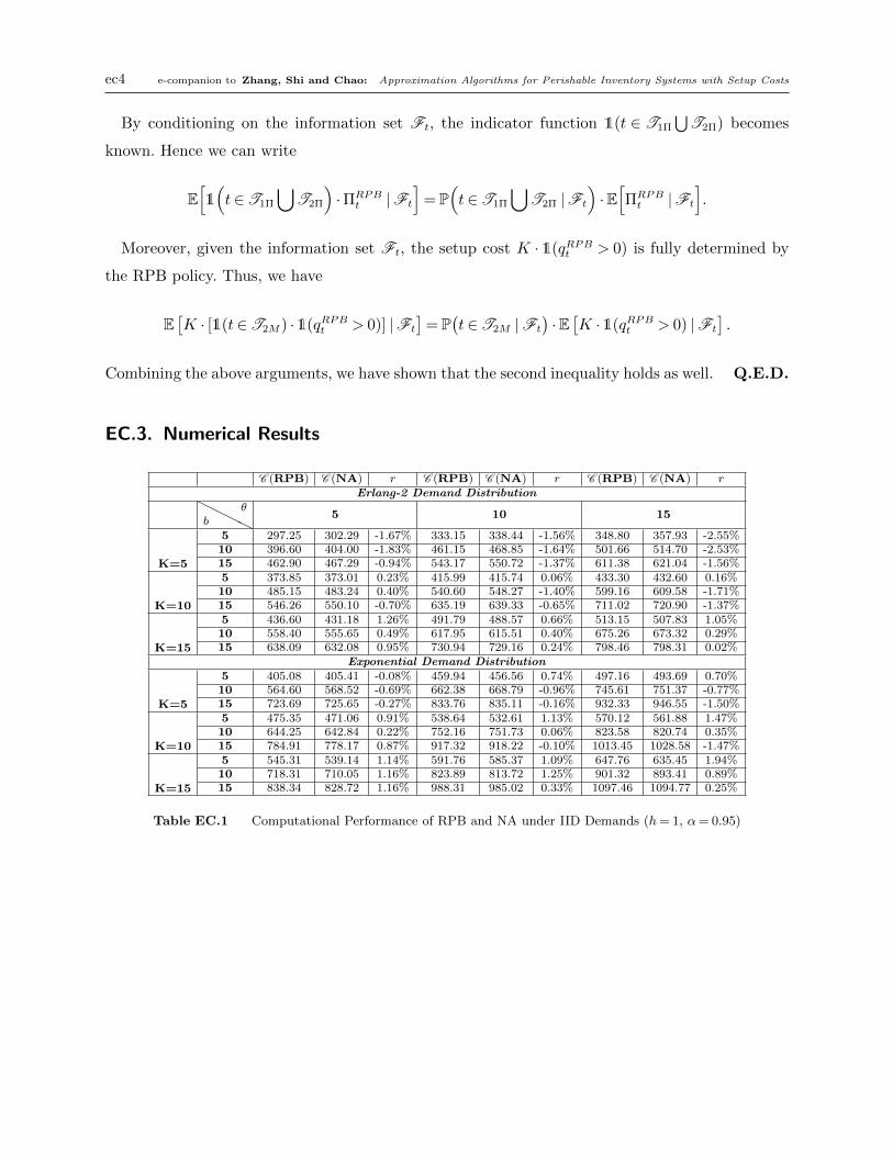
5.2. Numerical Results
Table EC.1 from the electronic companion summarizes our numerical results for the i.i.d. demand
setting. The performance ratio is very small for all test instances, which suggests that the perfor-
mance of RPB is comparable (in fact slightly better but not statistically significant) to that of NA
under i.i.d. demands. This also suggests both RPB and NA perform extremely close to optimality
(in that NA’s error is on average under 1% of the optimal solution). We also notice that both
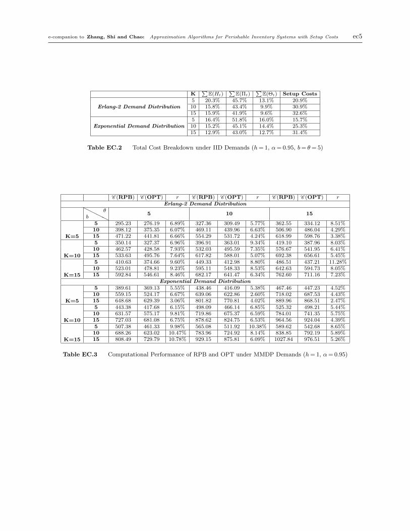
algorithms perform better when the setup cost is relatively small. Table EC.2 provides the total
cost breakdown for the i.i.d. demand setting (varying the values of K while fixing b= θ = 5). We
observe that the setup cost component accounts for a significant portion of the total costs, and
the percentage of setup costs increases in K. The ordering frequency is around 70% to 80% with
m= 2, and decreases in K.
Table EC.3 summarizes our numerical results for the correlated demand setting. The performance
ratio is small for all test instances, with average error under 7% and maximum error of 11.28%.
This indicates that the RPB policy performs well, and it is significantly better than the theoretical
worst-case performance guarantee.
Under both the i.i.d. and correlated demand settings, our numerical results suggest that the
performance of RPB is rather insensitive to b or θ, but improves as K gets smaller. We also test the
stability of RPB – the coefficient of variation of the total costs due to randomization. We consider
the case with exponential demand with mean 10, and evaluate the costs of RPB (with randomized
Zhang, Shi and Chao: Approximation Algorithms for Perishable Inventory Systems with Setup Costs 17
decisions) for the same cost parameters and demand realizations. We find that the coefficient of
variation of costs (standard deviation divided by mean cost) is at most 1.57%, suggesting that the
adverse effect due to randomization is rather small and RPB is quite stable.
Supplemental Material
An electronic companion to this paper is available at http://or.journal.informs.org/.
Acknowledgments
The authors thank the area editor Chung-Piaw Teo, the anonymous associate editor, and two referees for
their constructive comments and suggestions, which helped improve both the content and the exposition of
this paper significantly. The research of Huanan Zhang and Cong Shi is partially supported in part by NSF
grants CMMI-1362619 and CMMI-1451078. The research of Xiuli Chao is partially supported by NSF grants
CMMI-1131249 and CMMI-1362619.
ReferencesBox, G. E. P., G. M. Jenkins, G. C. Reinsel. 2008. Time Series Analysis: Forecasting and Control . Wiley, Fourth Edition.
Chao, X., X. Gong, C. Shi, C. Yang, H. Zhang, S. X. Zhou. 2015a. Approximation algorithms for capacitated perishable
inventory systems with positive lead times. Working paper, University of Michigan, Ann Arbor. Available at http:
//www.umich.edu/~shicong/papers/perishable2.pdf.
Chao, X., X. Gong, C. Shi, H. Zhang. 2015b. Approximation algorithms for perishable inventory systems. Operations Research
63(3) 585–601.
Essary, J. D., F. Proschan, D. W. Walkup. 1967. Association of random variables, with applications. The Annals of Mathematical
Statistics 38(5) 1466–1474.
Fries, B. 1975. Optimal ordering policy for a perishable commodity with fixed lifetime. Operational Research 23(1) 46–61.
Gallego, G., O. Ozer. 2001. Integrating replenishment decisions with advance demand information. Management Science 47(10)
1344–1360.
Heath, D. C., P. L. Jackson. 1994. Modeling the evolution of demand forecasts with application to safety stock analysis in
production/distribution system. IIE Transactions 26(3) 17–30.
Karaesmen, I. Z., A. Scheller-Wolf, B. Deniz. 2011. Managing perishable and aging inventories: Review and future research
directions. G. Karl Kempf, Pınar Keskinocak, Reha Uzsoy, eds., Planning Production and Inventories in the Extended
Enterprise: A State of the Art Handbook, Volume 1 . International Series in Operations Research and Management
Science, Vol. 151 (Springer, New York), 393–436.
Levi, R., G. Janakiraman, M. Nagarajan. 2008. A 2-approximation algorithm for stochastic inventory control models with
lost-sales. Mathematics of Operations Research 33(2) 351–374.
Levi, R., M. Pal, R. O. Roundy, D. B. Shmoys. 2007. Approximation algorithms for stochastic inventory control models.
Mathematics of Operations Research 32(4) 821–838.
Levi, R., C. Shi. 2013. Approximation algorithms for the stochastic lot-sizing problem with order lead times. Operations
Research 61(3) 593–602.
Lian, Z., L. Liu. 1999. A discrete-time model for perishable inventory systems. Annals of Operations Research 87(0) 103–116.
Lian, Z., L. Liu, M. F. Neuts. 2005. A discrete-time model for common lifetime inventory systems. Mathematics of Operations
Research 30(3) 718–732.
Zhang, Shi and Chao: Approximation Algorithms for Perishable Inventory Systems with Setup Costs 18
Nahmias, S. 1975. Optimal ordering policies for perishable inventory-II. Operational Research 23(4) 735–749.
Nahmias, S. 1976. Myopic approximations for the perishable inventory problem. Management Science 22(9) 1002–1008.
Nahmias, S. 1977. Higher order approximations for the perishable inventory problem. Operations Research 25(4) 630–640.
Nahmias, S. 1978. The fixed charge perishable inventory problem. Operations Research 26(3) 464–481.
Prastacos, G. P. 1984. Blood inventory management: an overview of theory and practice. Management Science 30 777–800.
Shi, C., H. Zhang, X. Chao, R. Levi. 2014. Approximation algorithms for capacitated stochastic inventory systems with setup
costs. Naval Research Logistics (NRL) 61(4) 304–319.
Brief Bio:
Huanan Zhang is a Ph.D. candidate in the Department of Industrial and Operations Engi-
neering at the University of Michigan. His primary research interest lies in stochastic optimization
and online learning problems with applications to inventory and supply chain management, and
revenue management.
Cong Shi is an assistant professor in the Department of Industrial and Operations Engineering
at the University of Michigan. His research lies in stochastic optimization and online learning theory
with applications to inventory and supply chain management, and revenue management. He won
first prize in the 2009 George Nicholson Student Paper Competition.
Xiuli Chao is a professor in the Department of Industrial and Operations Engineering at the
University of Michigan. His recent research interests include stochastic modeling and analysis,
inventory control, game applications in supply chains, and data-driven optimization.
e-companion to Zhang, Shi and Chao: Approximation Algorithms for Perishable Inventory Systems with Setup Costs ec1
This page is intentionally blank. Proper e-companion title
page, with INFORMS branding and exact metadata of the
main paper, will be produced by the INFORMS office when
the issue is being assembled.
ec2 e-companion to Zhang, Shi and Chao: Approximation Algorithms for Perishable Inventory Systems with Setup Costs
Electronic Companion to
“Approximation Algorithms for Perishable Inventory Systems with Setup Costs”
by Zhang, Shi and Chao
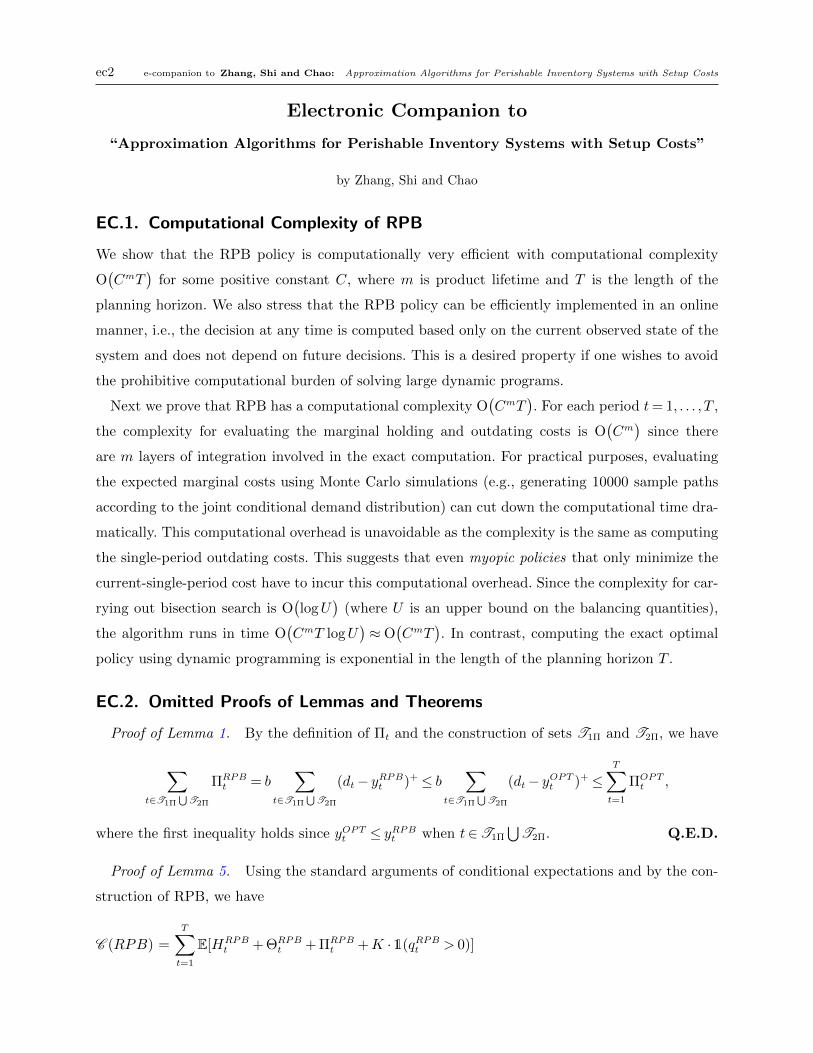
EC.1. Computational Complexity of RPB
We show that the RPB policy is computationally very efficient with computational complexity
O(CmT
)for some positive constant C, where m is product lifetime and T is the length of the
planning horizon. We also stress that the RPB policy can be efficiently implemented in an online
manner, i.e., the decision at any time is computed based only on the current observed state of the
system and does not depend on future decisions. This is a desired property if one wishes to avoid
the prohibitive computational burden of solving large dynamic programs.
Next we prove that RPB has a computational complexity O(CmT
). For each period t= 1, . . . , T ,
the complexity for evaluating the marginal holding and outdating costs is O(Cm)
since there
are m layers of integration involved in the exact computation. For practical purposes, evaluating
the expected marginal costs using Monte Carlo simulations (e.g., generating 10000 sample paths
according to the joint conditional demand distribution) can cut down the computational time dra-
matically. This computational overhead is unavoidable as the complexity is the same as computing
the single-period outdating costs. This suggests that even myopic policies that only minimize the
current-single-period cost have to incur this computational overhead. Since the complexity for car-
rying out bisection search is O(logU
)(where U is an upper bound on the balancing quantities),
the algorithm runs in time O(CmT logU
)≈ O
(CmT
). In contrast, computing the exact optimal
policy using dynamic programming is exponential in the length of the planning horizon T .
EC.2. Omitted Proofs of Lemmas and Theorems
Proof of Lemma 1. By the definition of Πt and the construction of sets T1Π and T2Π, we have
∑t∈T1Π
⋃T2Π
ΠRPBt = b
∑t∈T1Π
⋃T2Π
(dt− yRPBt )+ ≤ b∑
t∈T1Π⋃
T2Π
(dt− yOPTt )+ ≤T∑t=1
ΠOPTt ,
where the first inequality holds since yOPTt ≤ yRPBt when t∈T1Π
⋃T2Π. Q.E.D.
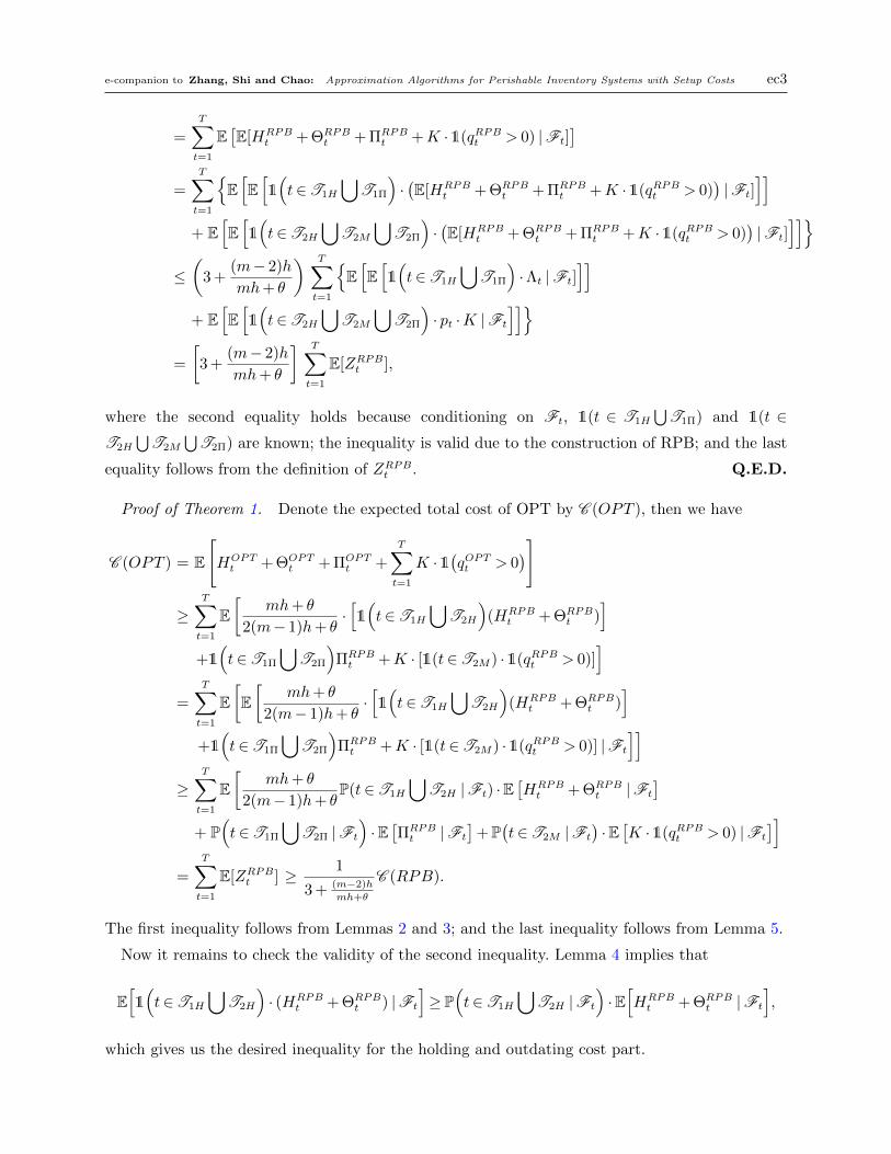
Proof of Lemma 5. Using the standard arguments of conditional expectations and by the con-
struction of RPB, we have
C (RPB) =T∑t=1
E[HRPBt + ΘRPB
t + ΠRPBt +K ·1(qRPBt > 0)]
e-companion to Zhang, Shi and Chao: Approximation Algorithms for Perishable Inventory Systems with Setup Costs ec3
=T∑t=1
E[E[HRPB
t + ΘRPBt + ΠRPB
t +K ·1(qRPBt > 0) |Ft]]
=T∑t=1
E[E[1(t∈T1H
⋃T1Π
)·(E[HRPB
t + ΘRPBt + ΠRPB
t +K ·1(qRPBt > 0))|Ft]
]]+ E
[E[1(t∈T2H
⋃T2M
⋃T2Π
)·(E[HRPB
t + ΘRPBt + ΠRPB
t +K ·1(qRPBt > 0))|Ft]
]]≤(
3 +(m− 2)h
mh+ θ
) T∑t=1
E[E[1(t∈T1H
⋃T1Π
)·Λt |Ft]
]]+ E
[E[1(t∈T2H
⋃T2M
⋃T2Π
)· pt ·K |Ft
]]=
[3 +
(m− 2)h
mh+ θ
] T∑t=1
E[ZRPBt ],
where the second equality holds because conditioning on Ft, 1(t ∈ T1H
⋃T1Π) and 1(t ∈
T2H
⋃T2M
⋃T2Π) are known; the inequality is valid due to the construction of RPB; and the last
equality follows from the definition of ZRPBt . Q.E.D.
Proof of Theorem 1. Denote the expected total cost of OPT by C (OPT ), then we have
C (OPT ) = E
[HOPTt + ΘOPT
t + ΠOPTt +
T∑t=1
K ·1(qOPTt > 0
)]
≥T∑t=1
E[
mh+ θ
2(m− 1)h+ θ·[1(t∈T1H
⋃T2H
)(HRPB
t + ΘRPBt )
]+1(t∈T1Π
⋃T2Π
)ΠRPBt +K · [1(t∈T2M) ·1(qRPBt > 0)]
]=
T∑t=1
E[E[
mh+ θ
2(m− 1)h+ θ·[1(t∈T1H
⋃T2H
)(HRPB
t + ΘRPBt )
]+1(t∈T1Π
⋃T2Π
)ΠRPBt +K · [1(t∈T2M) ·1(qRPBt > 0)] |Ft
]]≥
T∑t=1
E[
mh+ θ
2(m− 1)h+ θP(t∈T1H
⋃T2H |Ft) ·E
[HRPBt + ΘRPB
t |Ft
]+ P
(t∈T1Π
⋃T2Π |Ft
)·E[ΠRPBt |Ft
]+P(t∈T2M |Ft
)·E[K ·1(qRPBt > 0) |Ft
]]=
T∑t=1
E[ZRPBt ] ≥ 1
3 + (m−2)h
mh+θ
C (RPB).
The first inequality follows from Lemmas 2 and 3; and the last inequality follows from Lemma 5.
Now it remains to check the validity of the second inequality. Lemma 4 implies that
E[1(t∈T1H
⋃T2H
)· (HRPB
t + ΘRPBt ) |Ft
]≥ P(t∈T1H
⋃T2H |Ft
)·E[HRPBt + ΘRPB
t |Ft
],
which gives us the desired inequality for the holding and outdating cost part.
ec4 e-companion to Zhang, Shi and Chao: Approximation Algorithms for Perishable Inventory Systems with Setup Costs
By conditioning on the information set Ft, the indicator function 1(t ∈ T1Π
⋃T2Π) becomes
known. Hence we can write
E[1(t∈T1Π
⋃T2Π
)·ΠRPB
t |Ft
]= P(t∈T1Π
⋃T2Π |Ft
)·E[ΠRPBt |Ft
].
Moreover, given the information set Ft, the setup cost K · 1(qRPBt > 0) is fully determined by
the RPB policy. Thus, we have
E[K · [1(t∈T2M) ·1(qRPBt > 0)] |Ft
]= P(t∈T2M |Ft
)·E[K ·1(qRPBt > 0) |Ft
].
Combining the above arguments, we have shown that the second inequality holds as well. Q.E.D.
EC.3. Numerical Results
C (RPB) C (NA) r C (RPB) C (NA) r C (RPB) C (NA) rErlang-2 Demand Distribution
HHHHbθ
5 10 15
K=5
5 297.25 302.29 -1.67% 333.15 338.44 -1.56% 348.80 357.93 -2.55%10 396.60 404.00 -1.83% 461.15 468.85 -1.64% 501.66 514.70 -2.53%15 462.90 467.29 -0.94% 543.17 550.72 -1.37% 611.38 621.04 -1.56%
K=10
5 373.85 373.01 0.23% 415.99 415.74 0.06% 433.30 432.60 0.16%10 485.15 483.24 0.40% 540.60 548.27 -1.40% 599.16 609.58 -1.71%15 546.26 550.10 -0.70% 635.19 639.33 -0.65% 711.02 720.90 -1.37%
K=15
5 436.60 431.18 1.26% 491.79 488.57 0.66% 513.15 507.83 1.05%10 558.40 555.65 0.49% 617.95 615.51 0.40% 675.26 673.32 0.29%15 638.09 632.08 0.95% 730.94 729.16 0.24% 798.46 798.31 0.02%
Exponential Demand Distribution
K=5
5 405.08 405.41 -0.08% 459.94 456.56 0.74% 497.16 493.69 0.70%10 564.60 568.52 -0.69% 662.38 668.79 -0.96% 745.61 751.37 -0.77%15 723.69 725.65 -0.27% 833.76 835.11 -0.16% 932.33 946.55 -1.50%
K=10
5 475.35 471.06 0.91% 538.64 532.61 1.13% 570.12 561.88 1.47%10 644.25 642.84 0.22% 752.16 751.73 0.06% 823.58 820.74 0.35%15 784.91 778.17 0.87% 917.32 918.22 -0.10% 1013.45 1028.58 -1.47%
K=15
5 545.31 539.14 1.14% 591.76 585.37 1.09% 647.76 635.45 1.94%10 718.31 710.05 1.16% 823.89 813.72 1.25% 901.32 893.41 0.89%15 838.34 828.72 1.16% 988.31 985.02 0.33% 1097.46 1094.77 0.25%
Table EC.1 Computational Performance of RPB and NA under IID Demands (h= 1, α= 0.95)
e-companion to Zhang, Shi and Chao: Approximation Algorithms for Perishable Inventory Systems with Setup Costs ec5
K∑
E(Ht)∑
E(Πt)∑
E(Θt) Setup Costs
Erlang-2 Demand Distribution5 20.3% 45.7% 13.1% 20.9%10 15.8% 43.4% 9.9% 30.9%15 15.9% 41.9% 9.6% 32.6%
Exponential Demand Distribution5 16.4% 51.8% 16.0% 15.7%10 15.2% 45.1% 14.4% 25.3%15 12.9% 43.0% 12.7% 31.4%
Table EC.2 Total Cost Breakdown under IID Demands (h= 1, α= 0.95, b= θ= 5)
C (RPB) C (OPT) r C (RPB) C (OPT) r C (RPB) C (OPT) rErlang-2 Demand Distribution
HHHHbθ
5 10 15
K=5
5 295.23 276.19 6.89% 327.36 309.49 5.77% 362.55 334.12 8.51%10 398.12 375.35 6.07% 469.11 439.96 6.63% 506.90 486.04 4.29%15 471.22 441.81 6.66% 554.29 531.72 4.24% 618.99 598.76 3.38%
K=10
5 350.14 327.37 6.96% 396.91 363.01 9.34% 419.10 387.96 8.03%10 462.57 428.58 7.93% 532.03 495.59 7.35% 576.67 541.95 6.41%15 533.63 495.76 7.64% 617.82 588.01 5.07% 692.38 656.61 5.45%
K=15
5 410.63 374.66 9.60% 449.33 412.98 8.80% 486.51 437.21 11.28%10 523.01 478.81 9.23% 595.11 548.33 8.53% 642.63 594.73 8.05%15 592.84 546.61 8.46% 682.17 641.47 6.34% 762.60 711.16 7.23%
Exponential Demand Distribution
K=5
5 389.61 369.13 5.55% 438.46 416.09 5.38% 467.46 447.23 4.52%10 559.15 524.17 6.67% 639.06 622.86 2.60% 718.02 687.53 4.43%15 648.68 629.39 3.06% 801.82 770.81 4.02% 889.96 868.51 2.47%
K=10
5 443.38 417.68 6.15% 498.09 466.14 6.85% 525.32 498.21 5.44%10 631.57 575.17 9.81% 719.86 675.37 6.59% 784.01 741.35 5.75%15 727.03 681.08 6.75% 878.62 824.75 6.53% 964.56 924.04 4.39%
K=15
5 507.38 461.33 9.98% 565.08 511.92 10.38% 589.62 542.68 8.65%10 688.26 623.02 10.47% 783.96 724.92 8.14% 838.85 792.19 5.89%15 808.49 729.79 10.78% 929.15 875.81 6.09% 1027.84 976.51 5.26%
Table EC.3 Computational Performance of RPB and OPT under MMDP Demands (h= 1, α= 0.95)