Application of Integral Transforms Str349 420

INTERNATIONAL CENTRE FOR MECHANICAL SCIENCES

COURSES AND LECTURES - No. 220

APPLICATION OF

INTEGRAL TRANSFORMS

IN THE THEORY OF ELASTICITY

EDITED BY

I.N. SNEDDONUNIVERSITY OF GLASGOW

SPRINGER - VERLAG W%CM WIEN - NEW YORK

DYNAMICS OF ELASTIC AND VISCOELASTIC SYSTEMS

WITOLD NOWACKI

Professor of Meohaniaain The University of Warsaw

1. Introduction

In this course of lectures we shall deal with the theory of two-

dimensional systems, both continuous and discrete. In Chapter I we

present general methods of derivation of the displacement differential

equations describing the considered systems and a method of their sol-

ution. We consider also, some particular cases, namely strings and

beams.

The differential equation of deflection of a string or a membrane

and on the other hand of a beam or a plate, have been derived on a common

basis, namely the principle of virtual work implying the Hamilton prin-

ciple.

Moreover, we present a unified procedure for solving the differen-

tial equations describing transverse vibrations of strings, membranes

and beams and plates. This procedure concerns dynamic problems and

the solutions of static problems constitute a particular ca~e.

350 W. Nowacki

The above general method consists in making use of the Green

function in solving the differential equations for deflections. We

shall prove that a determination of the deflection of a structural

element may be reduced to an integral expression containing the external

loading and initial conditions, multiplied in an appropriate manner by

the Green function.

Another important problem consists in the determination of the

Green function. In order to unify this procedure we consistently apply

integral and finite transforms.

In dynamic problems we first use the integral Laplace transform

with respect to the time t, in order to eliminate the time from the

differential equation for deflection. Next, we make use of the Fourier

transform or a finite transform, depending on the prescribed boundary

conditions. Thus, for a plate strip simply supported on its boundaries,

we first apply the exponential Fourier transform and then a finite sine

transform. The inversion of the integral transforms leads to the Green

function. We arrive at the final results by substituting the Green

function into the integral expression examined in Sec. 4. The general

procedure presented in this Chapter can be extended to more complicated

systems, e.g. shells and to discrete gridworks. Finally we demonstrate

an application of an analogous method to the problem of free and forced

vibrations of systems the material of which is viscoelastic.

2. The principle of virtual work and Hamilton's principle

Consider an elastic body subject to the action of external forces;

the latter include body forces and surface tractions. We assume that

the external loadings depend on position x and time t. These sources

produce in the body a displacement field u(x,t) and the associated with

this field state of strain e.. and stress a...to %3

Elastic and Viscoelastic Systems 351

In linear elasticity we define the strain tensor as follows:

tjj = i("- 4 + U4 ,'>' t»d = 1.2,3. (2.1)

The components of the state of stress are linear functions of strain.

The generalized Hooke law has the form

The quantities y,X are material constants called the Lame1 constants.

The above equations are completed by the equations of motion which are

derived from the fundamental principles of mechanics, namely the prin-

ciple of conservation of linear and angular momenta. They have the form

"Jtj + Xi = Pai* °ji = ai3* 5 e V* t>0' (2"3)

where X is the vector of the body forces, referred to a unit volume, p

is the density and u. = i the acceleration.

n2

Equations (2.1) - (2.3) constitute the system of equations of

linear elasticity. They should be completed by the boundary and initial

conditions. Assume that the surface A bounding the body consists of

two parts, A - A + A . On A there are prescribed displacements while

on A tractions. Thus, we have the boundary conditions

u.(x,t) = w.(x,t), x e A , t > 0,t - t - u ( 2 ^ }

a,Ax,t)nAx) = p^(x,t), x, e A , t > o,

where u. and p. are known functions.

The initial conditions have the form

u.(x,0) = /.(x), fi.(x.O) = ff.(x), x e V, t a 0. (2.5)

They express the fact that at the initial instant t = 0 the distribution

of the displacement field /.(x) and its velocity gAx) are prescribed.

The principle of virtual work and Hamilton's principle are of a

fundamental importance in deriving the differential equations for the

vibrations of strings, beams, membranes, plates and shells.

352 W. Nowacki

The principle of virtual work has the form

j(X.-P».)SuAV • J p.tuM - \oi;.Sc.AV. (2.6)

V Ao V

Here Su. is the virtual increment of the displacement, fie., the virtual

increment of strain. We assume that the above increments are arbitrary(2)

and sufficiently smooth (of class C ) and that they satisfy the

kinematic conditions on the surface A. We require thatthe virtaal increments 6M . vanish on the surface A and are arbitrary

t- uonAa.

The principle of virtual work states that the sum of the virtual

work performed by the body forces, inertia forces and surface forces in

arbitrary virtual displacements is equal to the virtual work of the

internal forces.

Introducing the concept of the work of strain

(2.7)hd7 = *J v<n (V V V

we write Equation (2.6) in the form

\(X.-pu.)6u.dV + f p.Su.dA = 6%r. (2.8)

V Aa

The integrand in the expression for the work of strain is a positive

definite quadratic form. The necessary and sufficient condition that

the integrand in (2.7) be of such a form is the following:

3X + 2n > 0, p > 0. (2.9)

Observe that for a static problem a l l causes and resulting displacementsdepend on position, i . e . on x. Equation (2.8) takes the form


far.6u.dK + I p.6u.dA = « V . (2.9')V A

a

On the basis of the principle of virtual work we can (by varying

the state of displacement) derive a very general minimum principle for

a non-stationary displacement field.

Let us consider an elastic body continuously changing its state

between the instants t - t\ and t - tj. Let us compare the true

displacements taking place in the body with the displacements u .t5u.,

the variations 6u. being chosen such that they vanish at the instants%

t = tj and t = *2 :

6u£(x,t1) = 0, 6ui(x,t2) = 0. (2.10)

If we integrate equation (2.9) over t from t\ to ti, we obtain

*2 *2 *2

*1

f Y f ffil/fdt = 6^dt - p dtii.6u.dV (2.11)

twhere

6& = pr.6u.dV + I p.6u.d/l.V \

The variation of the kinetic energy is given by the formula

6X = fpfi.6fi.dV = fp|r(fi.6u.)dV - fpu.6u.dVj u t * J Of *• u T* u

since

ju.u.dV.VV

Integrating 6K. from tj to t2, and bearing in mind the assumption (2.10)

we obtain

354 W. Nowacki

I 6X.dt = -pf dtfu.6w.dK. (2.12)J J J * *ti ti 7

Substituting from (2.12) into (2.11), we have

*2 *2

6 I CWE-JC)dt = J 6Adt. (2.13)

*l *1If the external forces are conservative they possess a potential and in

this case

f26 CW-K-C)dt = 0 (2.It)

Denoting by IT = TV - £ the total potential energy of the system we

present the Hamilton principle in the final form

f61 (v-K)dt = 0 (2.15)

*1It states therefore that the integral (2.15) takes an extremum value.

3. Transverse vibrations of simple one- and two-dimensional systems.

In this Section, on the basis of the principle of virtual work

and the Hamilton principle we shall derive the differential equations

for vibrations of a string and a membrane and the equation describing

the vibrations of a beam and a plate. We shall emphasize here the

evident analogies in the derivations.

(a) Consider a string in tension along the xi-axis between the points

A and B. The constant tension in the string is denoted by S and its

length by 1. Assume that in the xa-plane a load q(,x,t) acts per unit

length of the string. This loading produces a deflection of the string

w(x,t) in the arz-plane. We have assumed here that in the cross-section


of the string there occurs a homogeneous state of stress a = -r andSC2C /I

that the deflection of the string is independent of y.

q(x,t)

Fig. 3.1

*• S

In deriving the differential equation for the deflection of the

string we should remember that the derived equation is approximate, in

view of the simplifying assumptions made above.

To derive the differential equation for the deflection of the

string we have made use of the principle of virtual work (2.8) of Section

2. Neglecting the influence of the weight of the string (^ = 0) on

its deflection, we write Equation (2.8) of Section 2 in the form

I I

pii&wAdx + qSwdx = 60iA, A = Idyda. (3.1)

o o A

The quantity ~W~ is obtained on the basis of the following considerations.

Under the influence of the external loading the length it of a linear

element of the string undergoes an extension. The work of deformation

356 W. Nowacki

• 1

is the following:

I

(da-dx) = S(V-l). (3.2)

0

We have denoted by da the length of the element da; after the deformation.

Summing the above deformations we obtain the quantity "1/f - S(l'~l).

The absence of the coefficient J in the right-hand side of Equation

(3.2) is due to the fact that at the instant of application of the

loading the tension S already had its final value. Strictly speaking

we should write (3.2) in the form TV - (S+dS)(l'-l) where dS is the

increment of tension S due to the loading q. However, this increment

is very small as compared with S. Taking into account that

I{[1 + (ff )2]*" D«tef (3-3)

[ 3W 2li1 + (-r—) J in series we arrive at the

formula

I(f)2dx (a.4)

0

Since Or—)2 « 1 we have retained only the first two terms in the expansion

of the function 1 + (—-) j*. Performing the variation of the work of

deformation

0

we represent Equation (3.1) in the form

I

( 5 ^ . pA£± + qHwda: = s [ | > l l . (3.5)i 3iC2 8 * 2 LZX J°0

If the string is clamped at its ends x - 0 and x = I we have

v(O,t) = 0, w{ltt) = 0. (3.6)


In deriving the principle of virtual work we assumed that when the

displacements are prescribed, then 6M. = 0. In our case we have

prescribed displacements (3.6) at the ends of string and therefore at

these points we have 6w(0,t) = 0, &w(l,t) - 0. Consequently, the right

hadn side of Equation (3.5) is zero. In view of the arbitrariness of

the virtual displacement 6w, the left-hand side of the homogeneous

equation leads to the differential equation

• - q(.x,t) - 0, (3.7)

3a;2 3*2 o

0 < x < I, t > 0,

where we have introduced the notation

e2 = /pA, a - pA.

The differential equation for the transverse vibrations of the string

(3.7) should be completed by the boundary conditions and the initial

conditions

u(x,0) = f(.x), u(x,0) = g(x), 0 < x < I, t = 0. (3.8)

(£>) Consider now transverse vibrations of a membrane. By a membrane

we understand a plate whose thickness is very small compared with its

other linear dimensions. A membrane offers no resistance to bending.

It constitutes the two-dimensional counterpart of a string.

Consider a membrane in a homogeneous tension S in the plane 2:1X2»

with contour o. Assume that normal to the plane x\Xi there acts the

loading q(xitx2,t). Under the influence of the tension S and the load-

ing q there arises in the membrane a two-dimensional state of stress

(described by the normal stresses a\\ = 0^2 homogeneously distributed

over the thickness of the membrane); the membrane then undergoes a

deflection in the direction of the a:3-axis, denoted here by w(x\,X2,t).

Let us derive the equation of deflection of the membrane, on the

basis of the principle of virtual work, by varying the displacement

358 W. Nowacki

Equation ( 2 . 8 ) :

-IJ«-IjTzpuSwdd + Ufod/l = 6TV^. ( 3 . 9 )

A A

We have neglected here the influence of the weight of the membrane

(.X. = 0) on its deflection. Under the influence of the external load-

ing an arbitrary surface element AQ of the membrane undergoes a deflection.

Separating this element and subjecting it to the tension S we find that

its surface increases by the value of the integral jfsdu d«, where da is

an element of arc of the contour CQ and Au is the displacement in the

direction normal to the curve <3Q. The increment in the surface is

shaded in Figure 3.2. Taking into account that for every surface

element the work of deformation is the product of the tension S and the

increment of the surface, we have for the whole membrane

= S(.A • - > ! ) , (3.10)

Fig. 3.2


where A' is the area of the surface of the deformed membrane. Thus,

Equation (3.10) constitutes a complete counterpart of Equation (3.2).

In the expression for the work of deformation (3.10) S is the

initial tension. It changes insignificantly due to the action of the

external loading q(x\,a;2,t); this increment is very small indeed as

compared with the initial tension and can be neglected in the expression

(3.10).

It is known from differential geometry that the change in area of

the surface is given by the formula

-IIA

Expanding the integrand of (3.11) in series and confining ourselves

to small deflections we obtain

A

Let us now determine the variation of the work of deformation. We have

5 V = S\\w &W d4, o = 1,2. (3.13)

AThe integral appearing in the right-hand side of the expression (3.13)

can be transformed as follows:

6 V = sffftw <5u) - w SwjdA (3.It)e Jj »a »° »aa

A

Making use of the Green transformation in the plane we reduce (3.11) to

the form

6 V = S f|^5ud8 - S\\w 6WCL4, (3.15)

e Jan JJ ,aaa A

360 W. Nowacki

where —• denotes the derivative of the deflection along the normal toon

the boundary a. Introducing (3.15) into (3.9) we arrive at the equation

w(Su -ahi+q)SwM - \—5wdB = 0, (3.16),aa J an

A o

where a = ph is the mass per unit surface of the membrane. If on the

boundary o the displacement w(s) is prescribed, then titf - 0 on a. There

remains in (3.16) the first integral only. In view of the assumed

arbitrariness of the displacement $u within the membrane (3.16) leads to

the differential equation

• <?2-=- + q = 0, x 6 A, t > 0, x = (Xi,x2), (3.17')

or

e2v2u-u = -q/a, a2 = S/a. (3.17")

This is the differential equation for transverse vibrations of a membrane.

It should be completed by the boundary condition

w(a,t) = 0 , e e a, t > 0, (3.18)

and the initial conditions

u(x,0) = /(x), u(x,0) = g(x), x e.At t = 0. (3.19)

(a) The differential equation of the transverse vibrations of a rod.

We proceed to derive the differential equation governing the

transverse vibrations of a rod, on the basis of Hamilton's principle.

We calculate the work of deformation ti/", the kinetic energy X and the

variation of work of the external forces 6£> , i.e. the quantities which

enter into the variational expression (2.13).

The work of deformation has the form


• if. (3.20)

We neglect in the expression for liA the influence of the transverse

forces; it is very small for beams used in civil engineering structures,

the longitudinal dimensions of which are considerably greater than the

transverse ones. Talcing into account that

o = Ec .XX XX* XX

(3.21)

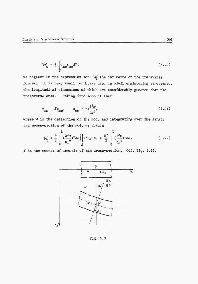
where w is the deflection of the rod, and integrating over the length

and cross-section of the rod, we obtain

I I

X = f f (—)2dx([*2dt/dS, = S f (^)2d*. (3.22)

I is the moment of inertia of the cross-section. (Cf. Fig. 3.3).

Fig. 3.3

362 W. Nowacki

The kinetic energy of the translational motion has the form

IK s £pj(w)2d7 - \a\ (.w)2dx, a = pA. (3.23)

V 0

Denoting by q the loading per unit length of the rod, we have

I6£ = (?6wdar. (3.24)

0

Hamilton's principle has the form

A d*f clxfe(—f - Ja(w)2] = f dtf qSwdx. (3.25)

Let us calculate the variations

I I

6| ( _ ) dx = 23x2 J 3x2 3a;2

0 0

Taking into account the identity

ix2 3a;2 Sxk dx 3a:2 3a; 3x3

we obtain

J Io ( ; da; - 2 owax t 2 • — — - 6W I . (3. 26)

J 3a;2 J 3x4 U x 2 3a; 3a;3 i°

Examine the second integral in Equation (3.25). Integrating by parts

with respect to t and taking into account that for t - t\ and t = ti we

have 6w = 0, then, in accordance with the assumptions made in deriving

the Hamilton's principle, we obtain

t2 I to I( f t ! !

^&\ dtl (w)2dx = - a dt w&wdx. (3.27)

*l t\

Introducing the above results in (3.25) we arrive at the relation


{ La*2 3a; 3a:3 J«1t

The second term vanishes as a result of the boundary conditions. If

the rod is simply supported at the cross section a; = 0,1 we have

W - 0, M - -El—- = 0 and also 6u = 0.3x2

If the end is fixed, then

W = 0, || = 0 and also 6u '= 0, 2|i = 0.

Finally, if the rod is free at the end, we have the conditions

M = -ETLSL =0, T = -BjL2. = 0.3a;2 3x3

Taking into account the above boundary conditions, we have from (3.28)

fdt[(H^ • -o)6wda; = 0.i i Sx1* 3t2ti 0

Since this relation has to be satisfied for every value of &W and

t{t\<t<ti) t we obtain the differential equation of transverse vibration

of a rod

EIUL + JOS. . q = 0, (3.29-)3a:1* 3t 2

- 2 8 ^ A :; _ „c2iÊ + „ = ( ? /n> C2 . ££ t 0 _ pAt (3.29")0

Equation (3.29') is associated with the two initial conditions

w(x,0) = f(x), u(x,0) = g{x), 0 .< x < I, t - 0. (3.30)

364 W. Nowacki

(d) The differential equation of the transverse vibrations of a

thin plate.

Considering the deformation of a thin plate, i.e. assuming its

thickness to be small in comparison with other dimensions, we make the

following simplifying assumptions:

a) points lying on a normal to the middle surface remain on the normal

to the middle surface after deformation;

b) during the deformation no strains are induced on the middle surface;

a) the influence of the shearing stresses 031,032 on the deformation

of the plate is neglected.

The displacements Wg(8 =1,2) are proportional to the angle

u - -x3w . (3.31)

The strains are then

E a 3 = J("a,S + We,a ) =- X 3 U,a0 ( 3' 3 2 )

Using the formulae for plane stress

°ae = 2ff(£a6 + l ^ V * f c ) ' e ^ = e 1 1 ^ 2 2 , O.33)

we obtain2Cte3

aag S " —[(1-V)u,ae + VV,/* ]' (3'3£°We introduce now the resultants of the stresses acting in the plate:

the bending moments are given by

Wa6 = j aaBXldX3> a'B = 1 | 2 i (3.35)

-h/z

Performing the integration, we have

»aB = "4(1-V)W + 6 w ]. (3.36)


where

Eh3N =

12(l-v2)

is the flexural rigidity of the plate.

Let us calculate the strain energy of the plate. Neglecting

the shearing stresses a 1 3, 023 and the normal stress 033 we obtain the

expression

KeW11'' a.B=l,2, (3.37<)V

A([ ( 1 + v ) oa8 0aB-^ am> V' (3'37M)V

where the integration is performed over the entire volume of the plate.

Replacing the stresses by the displacement w (Equation (3.3H)) and

performing the integration with respect to 3:3 (dV = dAdx$)t we obtain

([[(l-v^^v^)^. (3.38)A

The differential equation of the transverse vibrations of the plate can

be derived from Hamilton's principle

*2 *2

S| CW-K)dt = I 6kd*. (3.39)

The strain energy is expressed by Equation (3.38), the kinetic energy by

the formula

3C= Jo||(u)2d4, a = pfc, (3.40)

A

and the variation of the work done by external forces has the form

366 W. Nowacki

SC= Uq&wdA. (3.41)

A

Here q denotes the load acting on the plate.

Let us perform the variation of 5V:

5V =

A

= y\?[[v2uV2(6w)ci4

+ /V(l-v) 2 — - 6( ) o( ) S( ) \aA. (3.42)•'H 3xi3a;2 3xi3a;2 3 ^ 3a;2. 3x| 3a;2

Now, applying the two-dimensional Green's identity we obtain

JJ U J J 3n 3n

The symbol V4 denotes

The integral 6V" can be written in the form

/•/• s<7l 3?2 f«V" = -N(l-v) (•=— + •=—)d4 = -A?(l-v) (îcos^t<7 2sin^)ds, (3.44)

J J °3?1 d a - 2 J

-4 a

where

36w a2^ 36w 32W 36u S2^ 36u 32u3ar, 3a;2 3a;2 S jSiCj 3a;2 3#2 3a;j 3xj3x2

Let us transform the quan t i t i e s -s— , -5— appearing in Equations (9.4-5)

36w 36w a 36u . o. 36u 36u . Q SSw o

_ = — c o s ^ - _-s i n # , — = --emr? t -^cos^. (3.46)

Inserting now (3.45), (3.46) and (3.44) we obtain


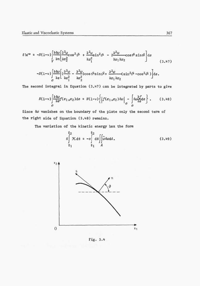
6-V" = --3np>V. da

(3.47)

L(i^.^ ) c o s^ s i n 2 5 ! +2 3x2

32U(sin2#-cos2*2)> ds.

The second integral in Equation (3.47) can be integrated by parts to give

3s (3.48)0 o

Since 6u vanishes on the boundary of the plate only the second term of

the right side of Equation (3.48) remains.

The variation of the kinetic energy has the form

2

I JCdt = -a (3.49)

Fig. 3.4

368 W. Nowacki

Thus, all the expressions occurring in Equation (3.39) are now known.

Hamilton's principle thus takes the form

I dt j j I [N^W+aw-q] SwdA (3.50)t, A

3n

.,(TaV2U ,_ ,3 ,32w 32!<K o . Q 32w i • ia 2 * \ L J A- N\ (1-v)— ( )cos^sin*1H (sm^v- -cos^-tr) \6wds =0

L ^« ^« ^««2 Q««2 Q*». Q « _ J3n 3s 3a;2 3x2 oxiax2

(* 1 2

We shall now prove that the integral over C the boundary of the plate

vanishes for homogeneous boundary conditions. Consider the curvilinear

contour of the plate C. The resultant of the stress, the bending moment

M and the torsion M can be expressed in terms of the moments Mj i,

as follows:

M = Inn

M - (M2z-Mn)sin2^ tWi 2cos2^. (3.51)YIS

Let us now introduce an invariant obtained by contraction of the

relations (3.36)

(3.52)

The transverse force is given by the formulae

The transverse force on the boundary C has the form

3w '

In view of (3.51), (3.52), (3.54) we represent Equation (3.50) in the form


V2

dt\\(NVkW+aw-q)6wdA = \\M (W)~ - V (w)&w]ds. (3 .55)] } j J L nn an n Jti A C

oM(w)where V (u) = QAw) t — r • The curvilinear integral on the right

hand side of Equation (3.55) vanishes, since all the boundary conditions

are satisfied. If the boundary is simply supported over its contour C,

then M - 0, w = 0 and therefore &W = 0.- If the boundary is clamped,

then W = 0, — = 0 on C and hence &W - 0 and —r— = 0. Finally, in theoYl an

case of a boundary free from tractions: M (u) = 0 and V' (u) = 0.

The quantity V (u) is the sum of the transverse forces acting on the

boundary (the so-called Kelvin-Tait boundary condition).Equation (3.55) takes the form

dt\\(NVHW+aw-q)6wdA = 0. (3.56)

ti A

In view of the arbitrariness of the virtual displacement &W the bracket

in the integrand should vanish and this equation holds for every instant

t where

Thus, the differential equation for the transverse vibrations of a

plate takes the form

a2vkw + w = j(xi,x2,t), (xitx2) e A, t > 0, (3.57)

where

a2 - N/a, a = ph.

The differential equation (3.57) should be completed by the initial

conditions

w(xuxz,0) = f(xltx2), u(a;i,a;2,0) = gtxi.a^), x e A, t - 0. (3.58)

Knowing the deflection surface W, we can determine the bending and

tors ional moments from the formulae (3 .36) .

370 W. Nowacki

4. General solution of differential equations of transversevibrations.

In the preceding section, on the basis of the principle of virtual

work and Hamilton's principle we derived the following differential

equations:

02*2±- w z - lq(x,t), a2 = S/Q, 0 = Ap, (U.I)x

c2V2w - w = q($i ,x2,t), a2 - S/a, a = ph, (4.2)

-a2LE - w = - ±q(x,t), a2 = EI/a, a = Ap, (H.3)

-c2VHw - w - - q(xi,xz,t)t o1 = N/a, a = ph. (4.4)

They describe the transverse vibrations of strings, membranes, beams and

plates, respectively. Only Equations (4.1) and (4.2) are hyperbolic.

These equations are to be completed by the boundary and initial

conditions.

Let us write Equation (4.1) - (4.4) in unified notation

- w = - 4?(x,t) xcvl, t > 0. (4.5)

This equation is completed by the boundary conditions appropriate for

each of the system, and the following initial conditions:

u(x,0) = /(x), w(x,0) = g-(x), x eA, t - 0. (4.6)

Equation (4.5) and conditions (4.6) concern two-dimensional problems.

However, in the case when the deflection is independent of the variable

#2 the above equation becomes one-dimensional.

We introduced before the Green's function G(x,x',i) satisfying the

differential equation

£>(G) - G = - -<5(x-x')6(£), x & A, t > 0, (4.7)


with the same boundary conditions as for the function W of Equation

(4.5) and with homogeneous initial conditions

G(x,x',O) = 0, G(x,x',0) = 0, x eA, t = 0. (4.8)

The Green's function can be regarded as the deflection due to the

action of an instantaneous concentrated external loading with intensity

equal to unity.

Taking the Laplace transform of both sides of Equations (4.5) and

(4.7) we obtain the equations

£(w) - (p2u - pf - g) = - i?(x,p), (4.9)

23(G) - p2G = - S(x-x'). (4.10)

We have made use here of the initial conditions (4.6) and (4.8) and we

have introduced the notations

00 00

W(x,p) = fu(x,t)<Tp*dt, GU.x'.p) = j G(x,x',t)e~p*dt.0 0

Let us multiply Equation (4.9) by ~G and Equation (4.10) by U,

subtract the results and integrate over the region A of the two-dimensional

system. Then we obtain

f[(p/(x)+9'(x))G(x,x',p)d4(x) + i.jj6(x-x')w(xip)dA(x).A A

Making use of the well-known theorem on the Dirac function

f[«(x-x')/(x)dA(x) = /(x 1),A

we arrive at the following formula for the transform of the deflection:

372 W. Nowacki

W(x',p) =

A

A A

We shall prove below that'the last surface integral transformed into a

curvilinear integral over the contour of the two-dimensional system,

vanishes in view of the homogeneous boundary conditions. Thus, after

inverting the Laplace transform and replacing x by x' we arrive at the

integral expression

t

Jr]G(xt,x,t)d4(xt). C4.12)

A

For a one-dimensional problem we obtain from (t.12) the formula

t I

w(x,t) = dt q(x',t-T)G(x',x,T)dx'

0 0

I

+ of fg(x')+f(.x') ~\G(x',X,t)dxf. (4.13)

0

In the above integral expressions the functions qt f, g are known. The

knowledge of the function G(x,x',t) makes i t possible to determine by a

simple integration over the variables x and t, the deflection of the

considered system.

Let us now prove that the expression


III = \G(x,x\p)S5(w(x,p))-iJ(x,p)£)(G(.x,x' tp))]dx (4.14)

o

in case of the one-dimensional problem, and the expression

I 2 = jj[G(x,KI,p)^(u(x,p))-w(x,p)^)(G(x,x',p))]d4(x), (4.15)

Avanish for the assumed homogeneous boundary conditions. Thus, in the

case of transverse vibrations of a string 35(w) = e 2 .3*2

Integrating by parts we obtain

I

dx2 dx2 I dx

If the string is clamped at the cross-sections a; = 0, I, then w = 0,

G = 0. Hence I± = 0. For transverse vibrations of a beam

a -a2- . Consequently, the integral expression (4.14) yields

after integration

1 -I( (OÛ _ J^l£)da. = «02|^.t»3l£..+S!!yl_E.My| , (4.17)•I da1* dxh L J0

0

The expression in parenthesis vanishes for all types of the boundary

conditions. If the beam is simply supported, then w - 0, w" = 0,

~G - 0, "5" = 0; if it is clamped, then w = 0, w' - 0, G = 0, G1 = 0.

Finally for a free end of the beam we have w" = 0, w"' - 0, ?" = 0,

G1" = 0.

Let us now proceed to transverse vibrations of a membrane. Here

= o2V2U and therefore

i^)ds = 0 (4.18)671

374 W. Nowacki

in view of the Green transformation on the plane. The integral (4.18)

vanishes in the case of a membrane supported on its boundary, for then

W = 0, ? = 0.

Consider finally the transverse vibrations of a plate. In this

case 35(w) = -e^^W and hence

J2 = a2 (wvNj - GVhw)dA. (4.19)

A

Transforming the above surface integral into a curvilinear integral over

the boundary a of the plate we arrive at the expression

;2| {V>i - V ^ - V l ? + V?)u]d<Vn(G)w\<L2

a

We have made use here of the transformations utilized in the derivation

of the differential equation for the plate deflection and the formulae

(3.51) and (3.54).

If the plate is simply supported on its boundary, then W = 0,

M (w) = 0 and ? = 0, M (?) = 0. If it is clamped, we have W - 0,

— = 0 and G - 0, — = 0. Finally, if the boundary is free of tractions

M (w) = 0, V (w) = 0 and M (?) = 0, V (G) = 0.nn n nn ' n

Thus, in all cases of homogeneous boundary conditions the integrals

11, 1% vanish. The deflection of the system is determined from Equation

(4.12) or (4.13). Consequently, we have reduced the solution of

differential equations for elastic systems to the determination of the

Green function.

5, The Green function for the transverse vibration of a stringof finite extent.


Consider the differential equation of the Green function G(x,x',t)

(e2_J —)G(x,x'tt) = - h{x-x')6(t) (5.1)3x2 3t2 °

with the boundary conditions

G(O,x',t) = 0, G{l,x\t) - 0, (5.2)

and homogeneous initial conditions

G(tt,x',0) = 0, Gte.jc'.O) = 0. (5.3)

Applying the Laplace transform to the Equation (5.1), we obtain

! ' ) . (5.4)d*2 ' - - o

Now perform over (5.4) the finite sine transform:

G(x,x',p) = j) G*(n,x% ,p)sinana; (5.5)

n=l

I

G*(.n,x',p) = "G(,X,X' ,p)sina xdx, a = y. (5.6)

0

Multiplying both sides of Equation (5.4) by sina x and integrating from

0 to i, we obtain

I If (02^L. - p2)G(a:,a;

I,p)sina xAx - - - 6(a-a:?)sinonaxia; (5.7)

i dx2 0

Integrating by parts gives

. xdx - a. [(-l)n+1G(l,a:t,p)+G(O,a;',p)]-a 2G*(n,a:',p). (5.8)

o d x2

The quantity in square brackets on the right side of relations (5.8)

376 W. Nowacki

vanishes since the boundary conditions are homogeneous.

Introducing the notations (5.5) we obtain

.<p-}W\n^B' ,p) - TSina x'. (5.9)

Let us now invert the finite sine transform

00

ina x'sina xl-, (5.10)a / p -> o

^—f patera zn-X * n

and subsequently the Laplace transform. Taking into account that

£ ( s—)M M

we are led to the solution in the series form

_-, sina x'sina xG(x,x',t) = •=£/ 2-sinui t, ai = a c. (5.11)

oL£_ , cx n yi n

n-l n

Consider the differential equation of the deflection of the string

(O2_!i _ _i5)(1)(a.ft) = _ lq{Xtt) (5.12)3a:2 3t 2 o

with appropriate boundary conditions, and in i t ia l conditions

w(O,t) - w(l,t) - 0, w(a,o) = f(x), W(K,0) = ^(x). (5.13)

The solution of the Equation (5.12) has the form

t I I

w(x,i) = \di\q(x' ,t)G(x' ,x,t-T)dx<+a \{g(x')+f(x')-^r\G(.x' ,x,t)dx<. (5.14)J ) 1 °v

0 0 0

Consider the case of the forced vibrations (<7 0, /=0, g=0)\

t I

w(x,t) = UTLW ,t-i)G(x' ,x,T)dx'. (5.15)

0 o

Suppose that at £ there acts a concentrated force which varies in time,


v i z .

qix,t) = F(t)6(x-Z), 0 < x, £ < I. (5.16)

Introducing (5.16) into (5.15), we obtain

t

wix,t) = I F(T )<?(?,z,t-t)dT. (5.17)

0

If Fit) - Hit), where Hit) is the Heaviside function, i.e.

{0 for t < 0,

1 for t > 0,

we obtain for the particular case

. <-> sina £sina xwix,t) = -^-> 2-(l-cosw t). (5.18)

n-1

Locate now at 5 an external periodic concentrated force

qix,t) = 6(a;-5)cosut, u> ={ u . (5.19)

Introducing (5.19) into (5.17) we obtain the following formula

wix,t) = -if-/ ^-(coswt-cosw t). (5.20)

As a) -»• w , this relation takes the indeterminate form TT. Applying

the L'Hospital rule, we obtain

o, _sina xsina £azt V n «

i W

n=l

Formula (1.21) yields a steady increase of the deflection in time. It

is valid only for small values of t, and hence for small deflections of

the spring from equilibrium. This restriction is necessary, since the

differential equation of deflection of string was derived under the

assumption of small deflections as compared with the length of the string.

378 W. Nowacki

Consider one more particular case of loading of the string.

Suppose that a force

(H(t)S(x-Vt) for 0 < Vt < Iq(xtt) - -I (5.22)

t 0 for Vt > I

is moving along the string with a constant velocity V, from x = 0 to

x - I. Introducing (5.22) into formula (5.15), we finally obtain

£, sino xw(x,t) = — / (a fsina> t-u sina Vt). (5.23)

Slâ (a 2V2-u, 2) " » » »n=l n n n

This formula is valid for 0 < Vt < I. It yields the deflection at x due

to the action of a concentrated force moving along the string with

constant velocity V. It is readily observed that as 7 + 0 , Vt •*• 5 we

pass from the dynamic to the static problem.

From (5.23) we obtain

, _sina Csina xW(x) = —) 2-. (5.24)

n=l

In the following we assume that q - 0, g - 0 and / \ 0. From the

equation (5.14) and (5.11) we have

I2 P f

w(x,t) = -r/ sina xcosw £ f(a;')sina a'ds;1. (5.25)

n=l o

Suppose that there acts on the string a concentrated force P at a point

5. At time t - 0 we suddenly remove this static loading and the string

begins free vibrations. The deflection of the string is given, for

t > 0, by formula (5.25), in which we have to setCO

o p _ , sina a;sina g

fix) = «„<*) = — 7 — 2 «_ ( 5 # 2 6 )iLj. - 2

5 Z ~ aM=1 n

Introducing (5.26) into (5.25) we obtain


. 2pys inVc.sina

n=l nina^cosw^t, wn = a a. (5.27)

6. The Green's function for the transverse vibrations of a membraneof finite extent.

Consider the Green's function G(x,x',t) satisfying the differential

equation

(e2V2-32t)G(x,x',t) = - is(x-x')6(t), a2 = |, a=p/i, xS(x\,«2)(6.1)

with homogeneous initial and boundary conditions.

First let us discuss the problem of vibrations of a rectangular

plate.

Applying the Laplace transform to the Equation (6.1) we obtain

(<?2V2-p2)G(x,x',p) = - S(x-x'). (6.2)

Now perform over (6.2) the finite sine transform. Introducing the

notacions

1"2I I

,mja:|,»|ip) = G(xi,x2;x[,x^;p)s±nanxisin&mx2dx:idx2, (6.3)

0 0

1=1 m=l

n a\ m

we obtain the following form of Equation (6.2)

380 W. Nowacki

[°2 {an2 +8m2 )+p2^ GHn'm ;Xi >X2 ; p ) = 5 " i B V l s i M / 2 *

Inve r t i ng t h e f i n i t e s i n e t ransform in ( 6 . 5 ) g i v e s

00 00

G ( x , x ' , p ) = — - — / / - ^—sina arising a:2. (6.6)

kk°2K^Înverting the Laplace transform in (6.6) gives finally

00 00

1 z n = l m=l «

inBma;2sin(YMm<3t) ( 6 . 7 )

Y = (a 2 t 0 2 ) = .«m n m

Consider the case of forced vibrations. From the Equation (4.12) we

have

t

u(x,t) = I dTj|<7(x1,T)G(xl,x,t-T)cL4(x'). (6.8)

0 A

Suppose that a force

f F(.t)&(xi-Vt)6(x2-r)Z) for 0 < Vt < I,

qU,t) = \ (6.9)

1 0 f or Vt > Iis moving along the membrane with a constant velocity V, from x\ = 0 to

xx - a\ (along the line x2 = r\2) • Introducing (6.9) to Equation (6.8)

we obtain

t

w(x,t) = F(-[)G(.Vr,n2iXx,x2;t--r)dT. (6.10)

oIf Fit) - Hit), after integration with respect to t we have

uU,t) = > / 2 _ ( a Vsiny at.Qy s i n a v t )

z «=1 m=l 'nw n 'nm (6.11)


Consider the problem of free and forced vibrations of a circular

membrane. Assume that the forced and free vibrations depend only on

the variable r. We have to do with the axisymmetric problem of

vibrations. The solution of the differential equation

..',*), V2 = — t i !-, r = to?«f)*, (6.12)t ° 3r2 r 3r

has the form

at a

U(r,t) = |drl[q(rl,T)G(2'',r,t-T)dTta|[g(i'1)+f(r')^]G(rI,^Jt)dr'. (6.13)

0 0 0

If the Green's function G(r ,*>',£) is determined, the deflection w(r,t)

can be found from Equation (6.13).

The differential equation of the Green's function can be written

in the cylindrical coordinates

) - —}G(3r2 r 3r 3t2J

We assume that the boundary condition and the initial conditions are

homogeneous. Let us perform over the differential equation (6.It) the

Laplace transform, whence

I. (6.15)

dr2 r dr J a

We can solve the Equation (6.15) with use of the finite Hankel transform

a

G(r,r',p)nfo(a r)dr, (6.16)

o

,r\p) = — > G*(n,r',p)- — - . (6-17)2^_ [1 («-«)] 2

382 W. Nowacki

The parameter a should satisfy the transcendental equation

<70(cyz) = 0, n = 1,2,...,-. (6.18)

Multiply Equation (6.15) throughout by rJo(a. r) and integrate with

respect to r from 0 to a.

a_ a

2,d2 Id , 2a1 ( + )-pz

drz r drGrJ0(a r)dr - - M &(r-r' )reTo(oy)dr. (6.19)

Perform the integration by parts

a

a

rG^cyOdr. (6.20)

0

The expression in brackets vanishes for the upper limit, provided

Jo(a a) - 0; for r - 0 it vanishes always.

Taking into account Equation (6.20) we find that

c2(an2 t p2)G*(n,r> ,p) = J T V 0 ( B B I " ) . (6.21)

Performing the inverse Hankel transformation on (6.17), we obtain

^ rV0(ar'V0(iip)G(r,r',p) - -+-/ 2 S , (6.22)

aao^;(anVn»2)tri(ana)]»

Applying the inverse Laplace transformation, we arrive finally at the

result

2 vrV0(V')t70(V)

—sinu t,w = a o. (6.23)

In the particular case of a concentrated load q(rft) - -—6(r)H(.t)


we obtainp0 V* Jo(an

r

w(r,t) = — — / —-(1-coswt). (6.24)

7. Free vibrations of an infinite string and an infinite membrane.

Consider the homogeneous differential equation of the transverse

vibrations of the string (4.1). Assume that the string is infinitely

long, and that its motion is determined by the initial conditions

u(x,0) = f(x), w(x,o) = g(x), (7.1)

which mean that at the time t = 0 the string has deflection f(x) and

velocity g(x).

The solution of the equation

OL W =

has the form

;) s a( [^(«')+/(»')|^]G([ [flr(«* )+/(*'

Thus, we have to solve the equation

( c 2 — - — )G(x,x' ,t) = - ~6(x-x')6(t), -»<x«», *>0, (7.4)2 °3x2 3t2

with the homogeneous initial conditions and boundary conditions in

infinity: G •* 0 for \x\ -*•«>.

Performing the Laplace transform over Equation (7.4) for the above

homogeneous initial conditions, we obtain

! «2V3''»l8llp) = - -^(s;-*

1). (7.5)<te2

384 W. Nowacki

Further, perform over Equation (7.5) the exponential Fourier transform.

1 i-FxMultiplying both sides of Equation (7.5) by -=-e and integrating from

/2ir

-» to +•», we obtain

-i_[ (a2— _ p2)c(ar^',p)e*

5a:da: - - i -i- [ <5(x-x' )8iCsda:. (7.6)/2irJ.. d x 2 a /2irJ

Integrating the first term of (7.6) by parts gives

d G.igx

dxdx =

dx(7.7)

The quantity in square brackets on the right side of the relation (7.7)

vanishes, since at infinity both the deflection G and its derivative

-T- vanish. Introducing the notations

GU,x',p) = - M G(x,x',p)e^dx, (7.8)/2TTJ

G(x,x',p) •-*- G(S,xI,p)e"t'Ca:d5, (7.9)/2irJ

we transform Equation (7 .7 ) t o the form

p-)U = e • (7.10)a/2ir

Introducing the Fourier transform for the expression pG, we obtain

d?. (7.11)

Let us now invert the Laplace transform. Taking into account that


£ (-£ ) = COS5Ct,

p2+c252

we obtain

3t " 2iroJ cosiat e'îx~x1)iK. (7.12)

Moreover, in view of the relations

CO

cos^t = ôt+0'

Uoi), J e"in5d5 = 2t6(n)—00

we obtain the final for the solution (7.12)

H = ^[6(x-x<-ct)+6(.x-x'+et)]. (7.13)

Assume now, that u(a;,O) = g(x) - 0. Introducing (7.13) into the integral

expression (7.3) we have [93]]

w{x,t) - \

- l[f(.x-at)+f(.x+at)\. (7.m)

This is the d'Alembert solution of the wave equation of the string.

The Equation (7.14) can be interpreted in the following way. Let us

deflect the string to the form of the curve f(x) at instant t - 0, and

remove the forces which produced the initial deflection, without inducing

an initial velocity of the element of the string (i.e. g - 0). For

t > 0 the deflected form of the string is divided into two waves (the

waves ^f(x-at) and \f{x+ct)). One wave moves to the right with theS -

constant velocity a - (—)2, while the second moves to the left (Fig. 7.1).

Let us discuss the problem of free vibrations of an infinite

membrane. The equation of the transverse vibration of the membrane has

the form

386 W. Nowacki

t=0

Fig. 7.1

aV2w-u = 0, x e A, t > 0. (7.15)

Furthermore, we assume the following form for the in i t ia l conditions:-

w(x,0) = f(x), w(x,0) = g(x), x = (x!,x2) e. A, t = 0. (7.16)

The solution of the differential Equation (7.15) takes the form

GO ro

U(x,t) = of [ [g(x< )+fU' )~\G(x,x' ,t)dA(x'). (7.17)

The differential equation

82(C2y2 _ l_ ) G ( X ) X. j t ) - _ i6(x-X

2 - " 0(7.18)

is to be solved with the homogeneous initial conditions. We first of

all place the Dirac function at the origin of the coordinate system.

In this case the equation of transverse vibrations of the membrane

can be written in cylindrical coordinates


|W(l.,0,t) . - ± | H U « t ) , (7.19)

whereV2 - 5 1 . + 1 i_

3r2 r 8rC

2 =

Applying the Laplace transform to Equation (7.19) we have

(c2V2-p2)G(r,0,p) = - i | g i (7.20)

Denote by G(a,0,p) the Hankel transform of the function

f _G(a,0,p) = G(r,O,p)rer0(aj.)dr, (7.21)

0

and by G(r,0,p) the inverse Hankel transform

00

G(r-,O,p) = G(ct,0,p)a<7o(ou')da. (7.22)

Here we observe that

00

f r(SLL + I ^-)G(r,O,pV0(ar)dr = - a2G(a,0,p). (7.23)J dr^ v dro

Multiplying Equation (7.20) by rJo(<w), and integrating with

respect to r over the interval (0,<°), we transform Equation (7.20) to

the form

(c2a2

+p2)G(«,0,p) = i ^ . (7.2H)

Applying the inverse Hankel transform (7.22), we have

(7.25)

G(*,O,p) = ~2itc o pz+a'fl

Applying the inverse Laplace transform we arrive finally at the

relation

388 W. Nowacki

G(r,0,t) = £ ^ | tTo(ar)sinactda (7.26)

0

or

< (7.27)( 0 for at < r < «>

where r = (x2 + x 2 ) 5 .

Now, we remove the concentrated and instantaneous impulse to the point

x1.

We obtain

(7.28)f(c2t2-r2f 5 for 0 < v < at

- \2iroo "1 0 for at < v

where, now,

is the distance between the points x and x'

8. The Green's function G(x,x',t) for the transverse vibrationsof a rod.

Consider a rod of finite length I which undergoes forced and free

vibrations. Assume that at time t - 0 the deflection and velocity of

the rod are known, i.e. that

u(x,O) = f(x), w(x,O) = g(x). (8.1)

Thus we have to solve the differential equation

C 2 i ^ + y . 1 (Xtt)t « » . £ [ , a a M i (8.2)


with the initial conditions (8.1) and homogeneous boundary conditions at

the ends of the rod. The solution of the Equation (8.2) has the form

t I

w(x,t) = I dx] q(x' ,t-x)G(.x' &,x)ax'0 0

I

+ o \g(x')+f(x')^-\G(x',x,t)dx'. (8.3)

The starting point of our considerations is to solve the

differential equation of the Green function

(a-— + -—)G(x,x',t) = h(x-x')6(.t). (8.4)

The Green function must satisfy the Equation (8.4) with the homogeneous

initial conditions

,0) = 0, G(x,x',0) = 0, (8.5)

and the same boundary conditions as the function w(x,t).

Now consider the differential equation

^ » X * V ( x ) i X 4 = ^ . (8.6)

dx4 a2

the differential equation of harmonic free transverse vibrations. Apply

now to (8.6) the Laplace transform. The transformed equation (8.6)

takes the form

h p2t/'(O) + pfc"'(0) + W" (0), (8.7)

00

W(p) = [0

Now inverting the Laplace transform in Equation (8.7) and taking into

account the relations

390 W. Nowacki

(8 .8 )(2X2

P2 - X 2 p2+X2

r-l, 1 . 1 ,sinhXx-sinAxv 1 . , , , ..l^ ( ; = — ( ) = —V(Xx),

p^-X1* X3 2 X3

r-X, v > 1 /COshXx-cosXa:.. 1 . , , , ..

p^-X4 X2 2 X2

L-l( p2 ) = 1 (sinhX J ; t5inXx ) s i r ( A a ; ) |

p^-X4 X 2 X

XI ( -2 -—) = — (coshXar+cosXa;) = S(\x),p^-X1* 2

We a r r i v e a t t he fol lowing form of t h e s o l u t i o n of Equation ( 8 . 7 ) :

W(x) = W(0)S(\x)+ jW'(0)T(\x)+ p ^ ' ( ( W ( X a ; ) + i j ^ " ' (O)K(Xa;). ( 8 . 9 )

The solution (8.7) has a number of advantages. The constants

V(0), W1(O), W"(0), W" (0) appearing in it can be interpreted as the

deflection, the angle of inclination of the tangent of the deformed rod,

a quantity proportional to the bending moment and a quantity proportional

to the shear force, all in the cross-section x\ = 0. For arbitrary

boundary conditions, two of these quantities vanish.

Differentiating the function W(x) in formula (8.9), we obtain

W'(x) = (/(0)XK(Xx)tVl(0)5(Xx)+ h/"(0)T(,\x)+ ^-W"(0)U(\x),X X2

W"(x) - W(0)\2U(\x)+W'(.0)\V(\x)+W"(.0)S(\x)+ jW" (0)T(\x), (8.10)

W"(x) = W(O)\3T(\x)+W'(O)\2U( x)+W"(0nV(.\x)+W"' (O)S(Xx).

Making use of the solution (8.9) and the relations (8.10), we can, in a


very simple way, determine the frequencies of vibrations and their

corresponding modes.

Suppose that the rod is clamped at the cross-section x = 0 and

simply supported at x - I. The boundary conditions therefore are the

following:

W(0) = 0, W'(0) - 0, W(l) = 0, W"(l) s 0. (8.11)

In view of (8.9) and the second relation (8.10), and taking into account

the boundary conditions (8.11), we are led to the system of two equations

= 0,

w"(o)s(\i) + Y^"(o)r(xz.) = o.

Equating to zero the determinant of this system, we have

tanhB - tanB = 0 , g = XI. (8.12)

This is a transcendental equation having an infinite number of roots.

The f i rs t five are the following:

0! = 3,927, g2 = 7,069, S3 = 10,210, B4 = 13,352, B5 = 16,483

6 = * '- ^ z - t - x ) , V > 5 .

Since

the consecutive frequencies of vibration have the form

_ Bn2* _ £ « 2 R M S l 2

The mode of free vibrat ion W^xy), corresponding to the frequency u^ is

given by the formula (8 .9 ) .

Since (/(0) = fc"(0) = 0, we have

392 W. Nowacki

W (a?) - |y W"(O)U(\ x) + K- W" (0)V(\ x). (8.14)n X2 „ X3 „

We now prove that the modes of free vibration possess the important

property of orthogonality. Denote by w, , uu the frequencies and by

WAx)t WAx) the corresponding modes of vibration. Suppose that both

vibrations satisfy the same boundary conditions. The functions W-Ax),

WAx) satisfy the equations

• \l W = 0, - \*t VI- = 0. (8.15)

From these equations we obtain

I

0 dx dx 0

I

0

The expression in square brackets vanishes for both limits:

I

0

Since \k ? \l(uik ? ml), which has been assumed in view of two

different forms of vibration, Equation (8.16) is satisfied only if

I

WAx)Wt(x)dx = 0 k t I. (8.17)

0

This is the condition of orthogonality of the modes of free vibration of

a rod. Consider the integral

I[yAx)]2dx - y (8.18)

0

Bearing in mind that the mode of vibration contains a constant C,


we choose the l a t t e r in such a way that integral (8.18) equals unity.

In the case of the vibration of a rod simply supported at both

ends, we have

IC2 sin2a tfdx = y . a

7 = ~r»

0C2l /2

whence —=— = Y. If, therefore, we set C = /y , we obtain y - 1.

The functions

r, 1 \ /2 . knWAx) = / j s ina^ , afe = -j,

are called the normalised functions of free vibrations of a rod simply

supported at both ends.

In subsequent considerations we assume that the eigenfunctions

W-jix) satisfy the condition

[0 if k i IWAx)WAx)dx = 6,7 = { (8.19)* 4 Ki U if k s I.

Consider now the differential equation (8.H).

Apply the Laplace transform to Equation (8.t), whence

(c 2^- + p2)G(a:,a:',p) = h(x-x'). (8.20)

dx4 a

Let us now expand the function G into an infinite series of the

eigenfunctions W (a;), which satisfy the equation

2. - x^w = 0 (8.21)dz- n n

with the same boundary conditions as the function G and W. We introduce

the notation

394 W. Nowacki

I,p) = j G(a:,x',p)f/j (8.22)

G(x,x',p) = G*(n,x',p)Wn(x). (8.23)

n=l

This is a new f ini te transform. We have

M=l

= G*(m,x' ,p).ruil

n=l

We have used the condition of orthogonality for the functions W (x).

Now we multiply Equation (8.20) by W (x) and integrate from 0 to I.

I I(a2-— + p2)GW dx = -\ 6(x-x')W (x)dx. (8.24)

Since

dx = G ^dx+\W G"<-W 'G"+WI'G'-W"'G\! J djei+

L n n n n J 0

7 (8.25)

we have

(<J2xSp2)G*(n,a;',p) = ^ n ( *r ) . (8.26)

We now apply the inverse transform (8.23) to obtain Equation (8.26)


x->W(x<)W(x)G(.x<c',p) = -/— - (8.27)

aî p2+C

2X-n=l r n

Inverting the Laplace transform, we obtain

" V (x')WJx)G(,x,x',t) - -) -2 sinw t, u = cA2. (8.28)

i- i to n n n

a . nLet us examine forced vibrations: q i- 0, / = 0, g = 0. The Equation

(8.3) takes the form

1 t

w(x,t) = dx1 q(.x' ,*-T)G(X' ,a;,T)dT (8.29)

0 0

Z t

= I da;1] q(x' ,t)G(x' ,x,t-t)dT.

0 0

Suppose that along the rod there moves a concentrated force of intensity

Fit) with the constant velocity 7, i . e .f FU)5(.x-Vt) for 0 < Vt < I,

q(x,t) = •{ (8.30)1 0 for Vt > I .

We have assumed that q(.x,t) varies in time during the motion along the

rod. Introducing (8.30) into Equation (8.29) and taking into account

that

If Hx'-Vt)W (x')dx' = W (Vt),J n n0

we obtain for the delfection of the rod the formula

A t sinw (t-f)dt.,t) = i ) W (x)\ F(T)V (T7) j2 (8.31)

n=l 0

If F(t) = P0H(t), we have

396 W. Nowacki

W (x)rt*-/-rt—\ Vn(^)sinu.M(t-T)dx (8.32)«=1 " 0

In the particular case of a rod simply supported at both ends, we obtain

from (8.32)

00

2Pg r-i sina xw(x,t) = ) (a Vsim t-ia sina Vt). (8.33)

la 4 > (o^-u2) n n n nla -> (a^z-u)*)

n-1 n n n

This formula is valid for 0 < Vt < I. Formula (8.33) is valid also for

the case of a static concentrated force. It suffices to take V •+ 0,

and to assume that, in spite of the infinitely small velocity, the force

reaches point ? i.e. we set V-*-O,Vt-+£, sina Vt •* sinc*n5 in (8.33).

Hence

2P0 r-> sina £w Jx)=—T/ »n sina a;. (8.3H)

n=l n

Knowing the deflection of the rod w(x,t), we can calculate the bending

moment M(x,t) and the shear force T(x,t) by the formula

M = -£•!—, T(x,t) = -El—. ( 8 . 3 5 )3a;2 3x3

9. The Green's function G(x,x',t) for the transverse vibration ofa thin plate.

Let us investigate the problem: what frequencies u and what

vibrational modes lead to harmonic free vibration of a rectangular plate

supported along the edges. Assume that

W(.xux2,t) = W(xl,x2)e™t (9.1)


and insert the function (9.1) into homogeneous equation governing the

bending of the plate. This equation then takes the form

V*W - \*W = 0, X1* = £i, c2 = JL. (9.2)

c2 ph

Assume, also, that W(xi jc2) - X(x\ )Y(,x2), which corresponds with certain

types of boundary condition of a rectangular plate. In such a case

Equation (9.2) takes the form

X%l)Y(x2H2X"(.x1)Y"(x2)+X(xl)Yi'ir(x2)-\

kX<,x1)I(x2) = 0. (9.3)

The functions ^(xj), Y(x2) can be separated in the above equation for

instance, provided that either

X"(Xl) - -B2X(«i), XîxO = -B2r'(«l), (9.4)

or

F(xz) = -a2Y(.xx)t Yiv(x2) = -a

2T'(x2). (9.5)

The conditions (9.4) and (9.5) are fulfilled only by trigonometric

functions

f sing x2 ")) where a^ = — . & „ - -

cosa xj J (_ cos6 a;2

We assume that the plate is simply supported on the edges x2 = 0, a2.

This implies

7m(x2) = CsinB^, m = 1,2,...,«, (9.6)

since this function satisfies the conditions

I (0) = I (a2) = 0, X"(0) = r'(a2) = 0 (9.7)

for any integer m, and hence also the boundary conditions

ii.t) = 0.

In the case under consideration, Equation (9.3) takes the form

398 W. Nowacki

d-Jr 2 d 2 x h - e 4 )x - o.m

Apply the Laplace transform to Equation (9.8). We have

(P2-2e2)[p;r(o)+r(o)]+pr'(o)+r"(o)

X(p) = 22_o2 \2 _ , i (

( 9 . 8 )

( 9 . 9 ' )

i . e .

= ~(- )|"p^"(0) t2A2 p2-62 p 2 te 2 '

(9.9")

>2-62

where

Observing that

- 1 (

?2-62

6 2 = A2 + 6 2 .

, - l (

(p 2

+ e2

we find that Equation (9.9") , by means of the inverse Laplace transform,

yields

(9.10)= X(0)A(,xl)+X'(0)B(x1)+X"(,0)C(x1)i-X'" (O)D(xl),

where the following notations have been introduced:-

1 , - ^

>

B(xl) = ^(-^-sinh&t! + 6

2A2 6

C(x\) - (coshtei - c2A2

2A2 6

(9.11)


Observe that

i ) = X(.O)A(.x)+X'{O)B(x1)+X"(O)C(xi)+X"'(O)D(.x),

(9.12)

. Dm

where

Consider a plate with the clamped edges x\ - 0, <X\- In this case we

have

*(0) = X'(0) = X(ax) = X'taO = 0, (9.13)

and the solution (9.12) has the form

XUO = X"(0)C(xi) + X'" (O)D(a;i). (9.14)

Here the two first conditions of the set (9.13) have been used. The

remaining conditions lead to the system of equations

X(ai) = X"(0)C(ai) + r" (O)D(ai) = 0

X'iaO = r(0)C"(ai) + r"(0)C(ai) = 0.

This system does not lead to a contradiction if its determinant is equal

to zero, i.e. if

2(an) = 0.

Thus we are led to the relation

1 "1-)(6coth^ ecot^—) = 0.

(9.15)

400 W. Nowacki

The equation

&tanh-x~ + e t a n - y = 0 (9.16)

corresponds to the symmetric modes of vibration of the p l a t e , and the

equation

ficotanTj— ecotan-—- = 0 (9.17)

to the antisymmetric modes of vibration.

For a given value of 3 the consecutive value of A can be

° m run

calculated by means of Equations (9.16) and (9.17); furthermore the

consecutive frequencies of vibration are given by the formulau = e\2 (9.18)ran ran

The mode of the eigenvibrations is given by Equation (9.12)i, i.e.

= r'(0)C(ai)

• ] •(9.19)

D(ai)

In the particular case of a plate simply supported along the edges

x, - 0, a.\ we obtain

Since

we have

= °' En = 7 T ' n = 1'2'---'°

n ^ ran

A2 = a2 + B2, a = — .nm n m n a\

This leads to the result

u - a\ - (az+32) /-. (9.20)nm mn n n A/ a v' '

The mode of the eigenvibrations has the form

nvxi— . (9.21)


Consider two different modes of free vibrations of the plate

(satisfying the same boundary conditions), namely W. .(xi,x2) and

W*^(xi,X2) with the corresponding eigenvalues A., and A,-.

These satisfy the differential equations

From these equations we have

WidWkl)6A = aifXk)^y..Vkt6A. (9.23)

A A

But the left side of Equation (9.23) is equal to zero (see (4.2)1). we

have

A

Since X .. =/= X, 7 , Equation (9.24) is satisfied only if

ff..W.^dA = 0, (t / k, 3 t I). (9.25)

A

The eigenfunctions of the free vibrations of plates are orthogonal;

their coefficients are chosen to satisfy the condition

W2..dA = 1 . (9 .26)I'd

A

In the following considerations it will be assumed that the eigen-

functions satisfy both conditions (9.25) and (9.26).

Observe that the orthogonality property holds also for modes of

vibration which cannot be written in the form of a product

Consider a plate which undergoes forced and free vibrations.

402 W. Nowacki

Assume that at time t - 0 the deflection and the velocity of the plate

are known, i.e. that

w(x,0) = fix), u(x,O) = g(x), x S (xi,x2). (9.27)

The solution of the differential equation

c2tkw + w - -q(x,t)

takes the form

t

u(x,i) = IdTJL(xlst-T)G(x',x)T)d4(x') (9.28)

0 A

A

Now, we must solve the differential equation for the Green's

function G(x,x',t):

(c2V4 + 32)C(x,x',t) = -6(x-x')6(t), (9.29)

with the same boundary conditions as the deflection u(x,t) and with

homogeneous initial conditions.

Applying the Laplace transform to Equation (9.29) we obtain

(c2Vlt+p2)G(x,x',p) =-6(x-x'). (9.30)

Let us now expand the function G into a series of the eigenfunctions

J/..(x), which satisfy the Equation (9.2) with the same boundary

conditions as the functions W and G. We introduce the notation of

finite transform

TV-G(X! ,x2;x' ,x' ;p)WkAxi ,x2)dxldx2, (9.31)

0 000 CXI

'l,x'2;p)ykl<.xl,x2). (9.32)

k=l 1=1


Multiplying Equation (9.30) by ^ ( s ^ ,x2 ) and integrating over the

whole region of the plate, we obtain

(p2+o2^t)GHktl;xl,x'2;p) = ki<*{»*p. (9.33)

Making use of the inverse transform (9.32) and inverting the

Laplace transform, we obtain the following expression for the Green's

function of the rectangular plate:-

)V»l)-dr«"tt"tfXb' (9-34)fcsl 1=1 KL

Consider a particular case of forced aperiodic vibrations. Introducing

(9.34) into Equation (9.28) and assuming g = / = 0, we have

fc=i Z=i o o o w (9#35)

Suppose that the force q(x,t) moves with the constant velocity V along

the line x^ = H2J and hence that

0 < Vt < a\

0 for Vt > a\.

Inserting q(.x,t) into Equation (9.35.) and taking into account the relation

0 0

we arrive at the formula00 00

u(x,t) = i £ Tjia^l ^T)'*'W^T»r»2)JHjinuw(t-T)dT. (9.36)fe=i 1=1 o mkl

If Fit) = P0H(t), where ff(t) i s the Heaviside-step function, then

404 W. Nowacki

V, ,(Vt ,n2H:-siiW,,(t-T)dT . (9.37)

fc*l 1=1 o Kt

In the case of a plate simply supported along the whole boundary a

particularly simple expression for the deflection of the plate is

obtained. Since

we obtain after carrying out the integration indicated in Equation

(9.37)OO CO

w(x,t) = ) ) —[a.Ksiiw^t-w^sinaj/t]. (9.38)

0 < Vt < a.

If V •+ 0, and sina.Kt + sina,ni Equation (9.38) gives the statical

deflection of the plate produced by the force PQ located at the point

en oo

w(x,t) =

k=l 1=1 ^kTWl'

Having found the deflection surface, we can calculate the stresses

occurring in the plate with the aid of Equations (3.34).

10. Transverse vibrations of rods and plates resting on anelastic foundation

The differential equation of the transverse vibrations of a rod


res t ing on an e l a s t i c foundation has the form

• w = - ( q - r ) , c 2 = —, o = pA. (10.1)3a* a a

Assuming a linear relation between the resistance r of the foundation

and the deflection (Winkler's foundation), we have

r(x,t) = ht(x,t) (10.2)

where k is the foundation modulus. Thus Equation (10.1) takes the form

a2— + w + K2W = q(x,t), K2 - k/a. (10.3)

aa* a

Equation (10.3) is only an approximation to real conditions. It is

valid only for small deflections. The assumption on r(x,t) states that

the resistance v(.x,t) produces a deflection only in the section x while

in fact w(x,t) depends on the resistance at all points of the rod. We

assume also that during the deformation the rod is in contact with the

foundation over the whole length. It is therefore clear that Equation

(10.3) only approximately describes the phenomenon of vibration.

Consider now an infinite rod resting in an elastic foundation,

which at time t - 0 is subject to the instantaneous loading

q(x,t) = P06(a:)6(t).

To Equation (10.3) we first apply the Laplace transform with

respect to time and then the Fourier cosine transform. Inverting the

Fourier cosine transform, we have

P ° f

-( 0*8u3£I

The inversion of the Laplace transform involves serious

406 W. Nowacki

d i f f i cu l t i e s . In the par t icular case u(0,£) we obtain

(i:)l(tk (10.5)

where JT(Z) is the Bessel function of first kind of order J. For the

static case, we have

w(x) = e'^Ccosnxtsinrvc), n = (Sr)K x > 0, (10.6)8£Tn3 bI

The differential equation of the transverse vibrations of a plate

resting on an elastic foundation has the form

C 2VVK3+IC 2W = ±q(x,t), a2 = f, a = ph, KZ - k7Q. (10.7)

Consider the infinite plate resting on an elastic foundation,

subject to the static loading. The load q(r) = _^ _ is applied to the

infinite plate. The problem of determining the deflection of the plate

is an axisymmetric one.

PQ Sir) 3 2 1 3 2, i

atfy+rpw = , V2 = + , n = (^)cr. (10.8)

a 2nr 8r2 r 3r

Multiplying Equation (10.8) by rJ'o(cir) and integrating with respect to

r in the interval <0,°°>, we transform Equation (10.8) to the form

p0 _ r(c2a4+nlt)w(a) = — , w(a) = w(r)rJ0(.ar)dx>. (10.9)

0

Applying the inverse Hankel transform, we havep0

w(r) = , (10.10)

2j .SnVr2


or

v = (»<• + x|r. (10.11)

There keio(z) is the modified Kelvin function. Assuming PQ = 1 and

moving the concentrated force to the point a;1, we obtain

-•jbôf'c!)4]. r = [(si-a,1)2*^-^)2]*.

Consider a plate-strip resting on an elastic foundation, simply

supported at the edges xj = 0 , aj and subjected to the action of a

concentrated force qi.xtt) - P06(x1-xJ)6(32).

We have to solve the equation

P0 k k«(*!-«!)6(a2), U4 =

ao2 N

ou = —6(Xi-a;')6(x2), w4 = • = -. (10.13)

ac2 ^

Using the finite sine transform and the integral cosine transform, we

obtain

2P0 Jl, r cos&czdg rntW(x) = ) sina xjsina x. 1 , a = — (10.14)

o W+tn2Wn*> 2 *M

2-Y

The solution of the infinite integral has the form

cosBx2dB „ j /O~Y^2 fl-«n -

where

We must take the real part of the integral (10.15). In the particular

case k - 0, we have to do with the integral

408 W. Nowacki

r COSfJa^dP It= (1+a x2)e~anXz , x2 > 0. (10.16)

i (a 2+32)2 Ha 3 "On n

The deflection u(x) takes the form

nX2) -a x2 .e n •'sinot Xisi

u ( 5 } = 2SIiyZrir3 : L i e 'o»a ; 2 s i n an

a : i s i n arfn=l n

From (10.17) we obtain the Green's function

nX2sina x{sina ^1,0:2 > 0. (10.17)

c n=l n (10.18)

Applying the operator V2 to the function G(x,x'), we have

r > exp [-a (x2-xl)]V2G(x,x') = <j>(x,x') = - Jf) ^ sina aJxsina^x] (10.19)

n=l "

or

Differentiating the function ifi(x,x'), we obtain

(10.20)


Now we can determine the bending and twisting moment in the closed form

M U(G) = -il

The form of the shear forces is the following

(10.23)

"3a:2 " 3aj2*

11. Free vibrations of an infinite rod and of an infinite plate.

Consider the integral expression (4.13) for the special case:

q • o, g = 0.

SB

,t) = of /(*' (11.1)

We have to solve the differential equation for the Green's function

-V3'~ r ' , t ) = -6(a;-x')6(t), e2 = — , a = p/1. (11.2)

Let us perform over the differential equation (11.2) the Laplace

transform and further the Fourier exponential transform.

410 W. Nowacki

Inverting the Fourier transform, we have

pG(x,x' ,p) =2TTO

Now we invert the Laplace transform. Since

(11.3)

we obtain

(11.4)

The following relation will be employed

/2TT-00

Introducing (11.5) into the integral expression (11.1), we obtain

1 f/(*')[c air^-SL (11.6)

or

w(.x,t) -

In the particular case

f{x-x')\cos— t sirf^—|dx'.Hot

(11.7)

-x2,

"+az

i.e. when the initial curve has a prescribed form, we obtain from (11.7)

fa- e x p

4(a 4+e 2t 2)cos

atx2


t=0

t-N

Fig. 11.1

Figure 11.1 represents the graphs of the function w(x,t) for

consecutive values of parameter t. For the sake of comparison the

dotted line represents the propagation of a transverse elastic wave in a

string, for the same values of t. In the latter case we have two

"crests" propagated in the opposite directions, for a rod, however, such

a division does not occur.

Let us discuss the problem of free vibrations of an infinite plate

and confine our considerations to axisymmetric modes of vibrations.

Assume that the initial conditions depend on the variable r only, and

are independent of the angle 9. The equation of the transverse

vibration of the plate can be written in cylindrical coordinates,

namely

,t) + U(r,t) = 0. (11.9)

The equation (11.1) takes for the axisymmetric form of vibration the

412 W. Nowacki

form00

' ' ^ d r 1 . (11.10)

o

We have to solve the differential equation for the Green's function

(o2v2 + a2)G(r,r',t) = h(r-r')&(t). (11.11)

Let us perform over the differential equation (11.11) the Laplace

transform and further the Hankel transformation. After inverting, we

obtain

CO

~ = if r(J0(ar')aJ-0(ar)cos(a2ct)da. (11.12)

o

Introducing (11.12) into the integral expression (11.10) we obtain

CO CO

w(r,t) = r'/(r')dr' aJ0(ar')JQ(ar)cos(oa2t)da. (11.13)

0 0

Consider the Weber integral

Inserting v = —iat into Equation (11.14) and taking the real part

of the integral, we have

This procedure leads to the following final form of the formula for the

free vibration of the plate


i

1.0

/1)

f^ 0.5

**•—__

k w / f0

•n -0 —

- 7j = 3• •

Fig. 11.2

2ct(11.15)

Let the initial deflection of the plate equal

From the Equation (11.15) we have

w(r,t) = aexp(-2 i

This leads to the formula [

/o Dw{vtt) = exp( -

l+n:

(11.16)

(11.17)

414 W. Nowacki

where n = 4ct/ 2> P = r/a*

The deflection W for several values of the parameter n is shown

in Figure 11.2.

12. Transverse vibrations of viscoelastic rods and plates.

In formulating the stress-deformation relation of a viscoelastic

body, it is convenient to represent them in a form analogous to that of

the perfectly elastic body. In the latter the Hooke law has the form

The system of Equations (12.1) can take a different form, corres-

ponding to the representation of the deformation as a sum of volume and

shear deformations. Subtracting from (12.1) the quantity — 6 . .e,, , we

have

°a - hhfku= 2uev + (Xefc*" s V V (12-2)

Contracting in (l?.l), we obtain

akk = {3X + 2vHkk' (12'3)

In view of (12.2) the system of Equations (12.1) - (12.3) can be replaced

by the system of equations

s-• = 2ue.., (12.4)

s = 3Ke, (12.5)

where

'., K = X + | u .

(12.6)


s . . i s cal led the s t r e s s deviator and e . . the deformation deviator.i<a T-a

The stresses s.. produce a change in shape only, this fact being

expressed by formula (12.4), while the mean normal stresses produce a

change in volume. The equations contain two constants, the shear

modulus v - G and the bulk modulus K. We now proceed to a viscoelastic

body. Assuming that in all round tension (compression) the body behaves

as perfectly elastic, Equation (12.5) remains unaltered. Relations

(12.4) are generalized by adding to the right hand side a term represent-

ing the Newtonian viscosity, i.e. the term 2ne... Thus

%a

Equation (12.7) represents the Kelvin model. The quantity t - n/ is

called the retardation time.

The relation

* ^ t i = 2veid> e = 3Jfe, tp = n/y, (12.8)

occurs for the viscoleastic Maxwell body.

General stress-deformation relations for linear viscoelastic

bodies can be represented in a form analogous to (12.4) and (12.5), viz.

Pl(D)8..U,t) = P2(O)e..(x,t), (12.9)

P3(D)sU,t) = Pk(D)eU,t), x = (xi,x2,x3), (12.10)

whereN.

PAD) = 5 "4"V\ «f*> tQ.t. 1,2,3,4,n=0

n 8M

are differential operators and D = denotes the n time derivative,

a. are constant coefficients.

Assume that the viscoelastic body is in natural state for t < 0,

416 W. Nowacki

i.e. there are no stresses and deformations, and the loading is applied

at the instant t - 0. Under these assumptions we may apply to Equations

(12.9), (12.10) the one-sided Laplace transform.

s..(x,p) = 2p(p)e..(x,p) (12.11)

-7(x,p) = 3K(p)7(x,p), (12.12)

where

• P2(p) _ . i\(p)

vip) = , Kip) = i2Pi(p)

Observe that Equations (12.1) and (12.2) are of analogous structure to

Equations (12.4) and (12.5) for the perfectly elastic body. However,

in the latter, the quantities p, K appearing in Equations (12.t) and

(12.5) are constants, while in the case of viscoelasticity we are dealing

with functions of the parameter p. Equations (12.11) and (12.12) can

be solved with respect to the stresses. Thus, we obtain the relations

»), (12.13)

where

Tip) =

We haw-already indicated the analogy between formulae (12.13) and (12.1) .

The analogies may be employed in constructing the stress-deformation

rela t ions for plane s ta tes of s t r e s s , one dimensional s t a t e of s t r e s s ,

e tc .

In the plane s ta te of s t r e s s , we have for the e l a s t i c body

°aB = ~ r [ ( l ~ v ) e ae + V e 6 oi3~- l ' e = e H + e22, <>>(? = X,2 (12.14)

where„ _ )i(3X+2u)


For the plane state of stress in a viscoelastic body

° a 8 • — L ^ d - ^ + v ^ e J , <*. B = 1,2 (12.15)

the quantities B, v being expressed in terms of u(p), X(p) by the

formulae

9

X+vi 2(Xtu)(12.16)

The above elastic-viscoelastic analogy was announced by Alfrey and Lee.

To solve a dynamic problem of viscoelasticity we can use the corresponding

solutions of the perfectly elastic problem, replacing in the latter X, v

by X, u and inverting the Laplace transform.

Consider now an example of transverse vibrations of rods of visco-

elastic material. The differential equation of the transverse vibration

of a rod of perfectly elastic material (after applying the Laplace trans-

form) has the form

O2^H + p2y - (XiP) + pf(x) + g(x), (12.17)dx1* 0

where

w(x,p) = j e~ptw(x,t)dt, a = J^.0

For a viscoelastic body, a should be replaced by o(p), the latter being

a function of p, the parameter of the Laplace transform. The transformed

equation of vibrations of a viscoelastic rod has therefore the form

,p) + pfU)

For the viscoelastic body

418 W. Nowacki

P(p) - n(p)(3A(p)+2p(p))

I(p)+u(p)

Suppose that w, /(a;), g(x)can be expanded into a series of eigenfunctions

of the rod of perfectly elastic material, with the same conditions of

support as the rod under consideration:

w{x,p) */wHn,p)Wn<.x), fix) -y f(n)W (a),«=1 n=l

(12.19)

g(x) - x), q(x,p) -

M=l

The functions V ix) are orthogonal and normalized, and they satisfy the

equation

= 0,El

Introducing (12.19) into (12.18) we obtain

Introducing (12.21) into (12.19), we have

(12.20)

(12.21)

(12.22)

00

;'tp)V (ar'Jdx' (12.23)

Elastic and Viscoel.iv.i. Systems 419

We have now to carry out the required integration and then to invert in

(12.23) the Laplace transform. The difficulty of carrying out the

latter operation is due to the complicated form of the function C2(p).

Taking into account that, in accordance with relations (12.12) and

(12.13)

P1(.p)Pk(p)-P2(p)P3ip) _ P2(p)X(p) = , y(p)

we obtain

, . 3P2(p)P4(p)- 2 ( p ) = E(p)I _ I i IS , (12.24)

o o 2P1(p)Pl|(p)tP2(p)P3(p)

In the particular case of a Kelvin body, we have

Pi(p) = 1, P2(p) = 2 0 ( 1 + ^ ) , P3(p) = p, Pn(p) = 3Kp.

Hence

9G(l+t v)a2(p) ^ . (12.25)

° 3 + fd+t^p)

Introducing (12.24) into (12.23) and inverting the Laplace transform,

we arrive at the required function w(x,t). A considerable simplification

of the expression ~P-{p) follows if we assume that the material is

incompressible (K •* », v = j ) . Then, setting P^(p) •* « in formula

(12.24), we have

P2ip) ZGI4 - = ( 1 + t p ) - (12.26)2 a _ , . a 3*2 a P l ( p ) " °

Introducing (12.26) into (12.23) and inverting the Laplace

transform, we obtain the solution of our problem:

420 W. Nowacki

w(x,t) = > W (x)<{ I f(x')W (x')dx1—

n=l»ntfc% + •„] +

B2)J 9-U')A/n( (12.27)

IVs

^ u (1-0^)n=l n n o

where

U) t

= tann

Documents

Application of Integral Transforms Str349 420