Integral Transforms for You & Me Royal Observatory ... · Integral Transforms for You & Me Royal Observatory Edinburgh Institute for Astronomy J. Berian James March 2008. CONTENTS

Integral Transforms for You & Me

Royal Observatory EdinburghInstitute for Astronomy

J. Berian James

March 2008

CONTENTS

1. Rationale 1Example: Electronic circuitry 1Example: The Universe 3

2. Synopsis 4Integral Transforms are Linear Operators 4Summary 6

3. Fourier Transforms 6Definitions and Basic Theorems 8Discrete Fourier Transform 14Partial Fourier Transforms (Segue) 17Hermite Polynomials are Eigenfunctions of F 17Examples and Exercises 20

4. Laplace and Mellin Transforms 20Definition and Basic Theorems 20Initial Value Problems (supplementary) 23Enough Moments to Last a Lifetime 23Examples and Exercises 23

5. Hankel, Abel and Radon Transforms 23Definitions and Basic Theorems 24FA =H 27Projection–slice theorem 29Examples and Exercises 31

Appendix A. Reference Table of Transforms 32Hankel Transforms 33Abel Transforms 33Radon Transforms 33

F L H A R

INTEGRAL TRANSFORMS FOR YOU AND ME

1. RATIONALE

Integral transforms provide a way to solve otherwise intractable physical problems.

They work by expressing the equations of a physical system in a new form that can be

solved with simple computation. An example is the Laplace transform, which renders

a useful class of differential equations trivially sovlable, converting them into algebraic

ones instead. Another is the very well-known Fourier transform, which maps functions

of Cartesian coördinates to functions of frequencies, where the latter are often the more

interesting physical quantity. Still others allow the incorporation of the geometry of the

problem into the method of solution, such as the Hankel transform, which arises in

cylindrical coördinates, and the Abel and Radon transforms, which apply to functions

projected along one or more dimensions.

In justifying the appeal of integral transforms to physicists, this opening sortie in-

troduces a pair of problems amenable to solution by their use. Of course, they can’t be

solved properly ahead of introducing the transforms themselves; the intent is to explain

the problems in sufficient depth to see the manner in which transforms are useful.

1.1. Example: Electronic circuitry. Figure 1.1 shows an electronic circuit comprising

two resistors and one inductance coil in series, and another inductance coil in parallel,

powered from a single voltage source. The components of the circuits modulate the

input voltage in well-defined, but moderately complicated ways; most importantly, their

instanaeous effect on the voltage is proportional to the voltage itself.

The question is: given a constant input voltage V0 that starts at t = 0 and shuts down

at t = 1, what is the behaviour of the currents inside the two quadrangle loops of the

circuit? Using I1(t ) for the left-hand loop and I2(t ) for the right-hand loop, the equations

that govern the system can be written down using Kirchhoff’s voltage law1, viz.

L1d I1

d t+R1(I1 − I2)+R2I1 = V0 [1−H(t −1)](1.1)

L2d I2

d t+R1(I2 − I1) = 0,(1.2)

1This, along with the voltage–current relationships for resistors and capacitors, is assumed knowledge; any

substantial undergraduate physics text will provide them concisely and in short-order.

1

2 INTEGRAL TRANSFORMS

ñV (t )

�� L1 �� ÿ��

� L2

�� ÿ�� R1

�� óI1(t ) I2(t )

��

� R2

��

FIGURE 1.1. A circuit diagram composed of two resistors and two in-

ductors in a particular arrangements that can viewed as constructing

two separate voltage loops. The use of Kirchhoff’s voltage law allows for

the equations governing the time-dependent currents in the system to

be written down; these are solved painlessly with the use of the Laplace

transform.

where H(t) is the Heaviside step function. So, the physical system presents as a pair

of coupled ordinary differential equations, which can now be solved using the integral

transform of Laplace.

To demonstrate the use of the Laplace transform, a bit of high-level notation and a few

properties are introduced without justification. All we need to know about the Laplace

transform L is that

• it changes the variable t (and functions f (t)) to the conjugate variable s (and

functions L{

f}

(t ) = L(s)) via a particular mathematical operation2;

• it is linear, so that L{

a f (t )+bg (t )}= aL

{f}

(t )+bL{

g}

(t ); and

• it has a peculiar effect on differentials, viz. L{

d f (t )d t

}= sL(s).

The latter property is obviously salient. Acting with this operator on both sides of equa-

tions (1.1) and (1.2),

(L1s +R1 +R2)L {I1}−R1L {I2} = V0 [L {1}−L {H(t −1)}](1.3)

(L2s +R1)L {I2}−R1L {I1} = 0,(1.4)

gives a pair of simultaneous equations in L {I1} and L {I2} that can be solved in a

straight-forward algebraic fashion, such as with partial fractions, before taking the inverse

transform to recover both I1(t ) and I2(t ). Clearly though, our understanding is impaired

by not knowing explicitly what L {1}, L {H(t −1)} and so on amount to as functions. But

no matter—we can return to this application when our understanding has grown. It is

the methodology that is important, particularly the recognition that by establishing a set

2Those who abhor mystery can examine equation 4.1 on page 20 now.

INTEGRAL TRANSFORMS 3

of high-order operations and some rules to govern them, equations like (1.1) and (1.2)

can be solved without ever having to integrate.

Example: The Universe. The formation of cosmological structures proceeds from per-

turbations δρ to a uniform background ρ̄. On scales where (equivalently, at times when)

the perturbations are small relative to the background density (δρ¿ ρ̄), the evolution

of the perturbations is governed by linearised general relativity, though it can be (and

almost always is) usefully distilled into the Newtonian fluid equations. Perhaps the key

equation is a combination of the latter known as the growth equation

(1.5) δ̈ρ+2H δ̇ρ− [Pressure−Self-gravity

]δρ = 0,

where H , the Hubble parameter, is a central quantity in cosmology but not relevant to the

discussion at hand. This second-order differential equation arises in many different

contexts, e.g. physical systems involving springs, and the canonical solutions e±iωt

represent a mix of exponential growth and decay and osciallation, depending on whether

ω is real, imaginary or complex.

Because, however, the initial perturbations δρ(x, t = 0) are not known exactly as a

function of position, but only statistically, an exact solution is a strange and unattainable

goal. It is not the solution but the complicated expression in brackets that is the source

of interest. The reason for this is that the homogeneity and isotropy requirements of

cosmology—that there be no special places or directions in the Universe—mandate that

the evolution must depend on physical scale, rather than any absolute position. Indeed,

the terms for pressure and gravity can be unpacked as functions of physical wavenumber

k.

Scale and position are a Fourier transform pair, as are time and frequency. By per-

forming a Fourier transform on equations like (1.5), the resulting transformed equation

describes the evolution of distinct modes and is much less opaque. Indeed, what looks

like a single equation is actually a set of equations, one for each mode of the density field,

with all modes evolving independently. In this manner, cosmological perturbation theory

has developed to the point where its processes and predictions are fairly well understood,

and in good agreement with observations of the Universe. As the perturbations grow in

size, different modes begin to interact with their (Fourier space) neighbours. Though

the situation is now much less clean (read ‘non-linear’), the conceptual framework of

evolving and interacting density waves provided by Fourier analysis is still extremely

useful.

These two problems illustrate two different integral transforms, as well as two different

uses of integral transform techniques. In the first, the use of the transform is purely

functional—one almost doesn’t care that the transformation into the space of frequencies


has been made, so long as the property of transformed derivatives allow the differentials

in the equations to be finessed. In the second, however, there is a clear emphasis on

understanding the physical process through the kaleidoscope of the Fourier transform.

This is all by way of saying that integral transforms are useful! They are often quite

beautiful as well, and only occasionally unyielding. If you remain unconvinced, at least

read the synopsis before deciding it is not worth your while.

2. SYNOPSIS

This is a short course about integral transforms: what they are, what they can do for

us and how to make them do it. This is an integral transform:

(2.1) F (s)︸︷︷︸output

=∫ x2

x1

d x︸︷︷︸interval

K (x, s)︸︷︷︸kernel

f (x)︸︷︷︸input

;

it is composed of four objects—two specific functions (labelled ‘input’ and ‘output’) that

change depending on the problem we are addressing, and two slightly more general

objects (the ‘kernel’ and ‘interval’) that remain the same for a transform irrespective

of the input function. In that sense at least, the latter two objects—and the kernel in

particular—are what define a particular transform.

And there are lots of different transforms: you will have heard of the Fourier trans-

form at least, and perhaps some others like the Laplace, Hankel, Abel or Mellin trans-

forms; each of these corresponds to a particular choice of kernel. The interval is not so

fundamental—usually, it is chosen to be as wide as possible in order that the integral

converge, given the kernel; in practice, this means intervals like the real (−∞,∞) and

half-real [0,∞) lines.

In our workaday world, it is always the input and output functions that matter to us,

reflecting the important truth that for physicists and astronomers integral transforms

should be a tool. The worry is that this will make the contents of the rest of the course

look rather like a shopping list, but in fact the transforms are much more inter-related

than they might first appear, and woven throughout the notes is an argument about

how we can understand exactly what integral transforms are doing. The problems in the

rationale may have brought out some of this already. Summarised in a single sentence

(which is too short to be properly understood):

Integral Transforms are Linear Operators. This is a key point because it provides a way

to understand exactly what an integral transform does. They operate on function in

much the same way as (certain) matrices do on vectors, and the analogy can be made

very precise by introduction of the full mathematical nomenclature, which we of course

will not do. But the idea of a basis in linear algebra can be extended to the objects we


FIGURE 2.1. This unashamedly sentimental offering from popular

early-21st-century webcomic xkcd illustrates how some objects are

not amenable to integral transformation. © Randall Munroe.

call functions just as well as it is to the objects we call vectors. Viewed this way, it will

become apparent that the kernel of an integral transform plays the same rôle as the

change-of-basis matrix in linear algebra, though acting in a more general theatre than a

finite-dimensional vector space. The idea of transformation should therefore be seen as

an especially general one, and the fact that integral transforms in particular are being

studied here restricts our attention to functions.

Indeed, it isn’t possible to transform just anything. Figure 2.1 demonstrates in a light-

hearted manner that we are at least restricted to what we casually think of a mathematical

function. And there are further technical restrictions relating to the continuity of the

function—if it jumps about too much or has unreasonable large values—more generally,

the kernel determines what functions can and can’t be transformed. For example, the

kernel of the Laplace transform associates with each input function a ‘region of conver-

gence’ where the integral of transformation is well defined. Technical points such as

these play not a minor rôle in the study of integral transforms, much to our chagrin when

the intention is simply to use a transform to solve a problem quickly and without fuss.

But, there is much to be gained from understanding integral transforms in depth.


FIGURE 3.1. Two important figures in the golden age of French mathe-

matics, during which many early results in analysis, still in use today,

were put forward: Jean-Baptiste Joseph Fourier (1768–1830; left) and

Pierre Simon, Marquis de Laplace (1749–1827; right).

Summary. “That’s nice,” you’ll say, “and it’s interesting. But it’s probably not something

I’ll be using in my research.” Wrong. Wrong.

3. FOURIER TRANSFORMS

Starting in 1807, Fourier (Figure 3.1) introduced a method by which to decompose

periodic functions into a sum of trigonometric function of different frequencies, and

reasonable people would refer to this as the beginning of harmonic analysis. The flavour

of mathematics in Fourier’s time was very different to that of today, where for instance

physics is treated as a separate discipline, but the results are remarkably modern for a

time when the rigourous conception of ideas like ‘function’ and ‘integer’ were still around

the corner.

Here is a key passage3 from Fourier’s work on heat in solids, where in order to solve

the partial differential equation that results from consideration of the physical problem

. . . la valeur de y relative à x = 0 sera donnèe en fonction de y ; soit alors

φ=φ(y), on

φ(y) = a cosπy

2+a′ cos3

πy

2+a′′ cos5

πy

2+ . . .

3Mémoire sur la propagation de la chaleur dans les corps solides, as in Œuvre de Fourier (1888), pp. 218–219


multiplant de partet d’autre par cos(2i + 1)πy2 , et intégrant ensuite

depuis y =−1 jusq’à y =+1, il vient

ai =∫ +1

−1φ(y)cos(2i +1)

πy

2d y,

car il est facile de s’assurer que l’intégrale∫cos(2i +1)

πy

2cos(2i ′+1)

πy

2d y,

prise depuis y =−1 jusq’à y =+1, est nulle, excepté dans le cas de i = i ′,où elle est égale à 1.

All three equations contain what today we would consider to be very important ideas.

In the first, Fourier states that this function can be expressed as the weighted sum of

cosinusoids with particular frequencies (odd-integer multiples of π/2); in the second,

he shows how the weights a, a′ etc. can be calculated; in the third, he describes why the

decomposition works, and this is perhaps the most important of all. When the product

of two cosinusoids with different frequencies are integrated4 the result is zero. ‘Est nulle’

indeed. Though initially it is utterly unclear why (and it will only become apparent

as we move further on), this property means that the cosinusoids provide a unique

way to compose a function. It is the uniqueness that is the key to deconstructing and

reconstituting functions; in today’s language we would describe these building-block

functions as orthogonal.

The term ‘orthogonal’, which at first seems a curious throwback from geometry, be-

comes, following a bit of explanation, an eminently sensible choice. The idea of con-

structing an arbitrary function out of sets of other arbitrary functions is not compelling

on its own, because there is nothing to guarantee that such a construction can be done

uniquely. Here is an example of this unremarkable truth.

Let f (x) = x2 +x and S = {x, x2,2x2,4x}. The set S does not constitute an interesting

base for constructing f because the function can be formed from many combinations of

the elements (allowing for them to be multiplied by scalars; that is, Fourier’s a, a′ and so

on). For example, f (x) = 1 ·x2 +1 ·x or f (x) = 12 ·2x2 + 1

4 ·4x or f (x) = 3 ·x2 −1 ·2x2 +4 ·4x −15 · x or . . . ; obviously this is going nowhere fast. Consider instead the simpler set

S′ = {x, x2}, with which there is exactly one way to construct f (x) = 1 · x2 +1 · x.

The reason this uniqueness is a good thing can be understood with an important

analogy: if one imagines the two elements of S′ as representing axes, and the coefficients

by which the elements are multiplied to construct f as coördinates on those axes, we can

see that x and x2 are every bit as orthogonal as the two axes of the Cartesian plane—for

each point in the plane, there is exactly one set of coördinates that specify a point. On

the other hand, S emphatically fails to meet this criterion, because x and 4x are not

4Over any symmetric interval: in Fourier’s case −1 to +1; in general −∞ to +∞.


orthogonal, and for that matter neither are are x2 and 2x2. Thus, by using a sensible

basis like S′, all the machinery that would ordinarily by used for vectors (in real space),

like sums, dot products, projections etc., becomes accessible for use with functions as

well. Already, this is pretty deep stuff!

We may understand what orthogonality means intuitively using our geometric analogy,

but what about analytically? The third equation from Fourier’s passage spells this out:

two functions are orthogonal if the integral of their product vanishes.

(3.1) f and g are orthogonal ⇔∫ ∞

−∞f (x)g (x)d x = 0

The reason that this accords with the geometric interpretation will be postponed until

later—in fact, we will return to this theme again and again. For now, it is time to get on

with some practical ideas; but keep the geometric analogy in mind.

Definitions and Basic Theorems. The modern Fourier transform is an extension of the

original idea that was sketched out above. There, a function was expressed in a series of

sinusoidal functions. In fact, this is not completely general, as it includes only a discrete

set of frequencies, and can only be used to build up periodic functions. For this reason,

an expression like that of Fourier’s is referred to as a Fourier series (a finite, or countably

infinite, summation). If, however, we allow sinusoids of arbitrary frequencies, and not

just multiples of π/2, to be used as building blocks, all functions, periodic or not, can be

expressed this way.

The Fourier transform of f (x), then, is defined as an integral, not a sum:

(3.2) F (k) =F{

f (x)}≡ ∫ ∞

−∞f (x)e−i 2πkx d x;

and, because one good turn deserves another,

(3.3) f (x) =F−1 {F (k)} =∫ ∞

−∞F (k)e+i 2πkx dk

is the inverse Fourier transform. So it goes that

(3.4) F−1 {F

{f (x)

}}= ∫ ∞

−∞

[∫ ∞

−∞f (x)e−i 2πkx d x

]e+i 2πkx dk = f (x),

though this is by no means a trivial statement. The Fourier transform is also almost its

own inverse: F{F

{f (x)

}}=F 2{

f (x)}= f (−x); so identity is obtained after four, rather

than two, applications of F .

The appearance of the exponential function in the integral5 should not be too surpris-

ing once it is recalled that, e.g. cosk = 12

(e−i k +e+i k

), and so, given that both positive and

negative values are included in the bounds of the integral, one might easily imagine that

the exponential is representing the contribution of a sinusoid of particular frequency

k to the function f at particular value of x. By integrating over x, all the domain of f is

5Comparing with equation (2.1), we see that e−i 2πkx is the kernel of the Fourier transform.


incorporated; the output function F (k) is the contribution of each sinusoid of frequency

k to all of f . That is to say nothing more or less than that the function has been converted

(transformed, even) from a basis that almost always representing time or space, to a basis

of spatial scales or temporal frequencies.

Conditions for the existence of a Fourier transform are quite far removed from the

concern of physics, where every (temporal) signal and every (spatial) field has a source

that is often to do with something oscillating, and therefore must have a Fourier trans-

form. Likewise, though many functions do not have Fourier transforms, it goes with out

saying that these will be of rare interest to the physicist. Nevertheless, the conditions for

the existence of F are two-fold6:

• the integral∫ ∞−∞

∣∣ f (x)∣∣ exists;

• any discontinuous jumps in f are only finite in size.

These conditions are stated only to give some awareness of the limitations on the Fourier

transform, and will not be given consideration hereafter.

Table A.1 lists the Fourier transform of many function that arise commonly in physical

applications. These can be treated like tables of indefinite integrals that accompany

definitions of the integral calculus; a set of rules for modifying these functions extend the

availability of simple transforms even further, and these will now be described.

Theorem 3.1. Similarity theorem for the Fourier transform. If F{

f (x)} = F (s), then

F{

f (ax)}= 1

|a|F (s/a).

Proof.

F{

f (ax)} =

∫ ∞

−∞f (ax)e−i 2πkx d x

= 1

|a|∫ ∞

−∞f (ax)e−i 2π(ax)(k/a)d(ax)

= 1

|a|F (k/a)

�

This allows for a linear rescaling of the variable being transformed and the conversion

a → 1/a is significant—a compression of a variable corresponding to time (period)

amounts to a stretching in frequency.

6Of these two, the first is the most important, as it limits the lengths to which the vector–function analogy

that was outlined above can be drawn. Formally, the space of functions analogous to a vector space is

L2[−π,π], the space of square-integrable functions over the domain from −π to π; the functions ei nx provide

an orthonormal basis for L2[−π,π]. The area of mathematics concerned with such infinite-dimensional spaces

as these is called Hilbert space geometry, and it is useful in many areas of physics.


Theorem 3.2. Linearity of the Fourier transform. If F{

f (x)}= F (k) and F

{g (x)

}=G(k),

then F{

a f (x)+bg (x)}= aF (k)+bF (k).

Proof.

F{

a f (x)+bg (x)} =

∫ ∞

−∞(a f (x)+bg (x)

)e−i 2πkx d x

= a∫ ∞

−∞f (x)e−i 2πkx d x +b

∫ ∞

−∞g (x)e−i 2πkx d x

= aF (k)+bG(k)

�

This is a very important property that is general to integral transforms, and follows

from the linearity of the integration operator. Vectors also satisfy the linearity relation

under vector addition and scalar multiplication, which forms part of the correspondence

between (L2) functions and vectors.

Theorem 3.3. Shift theorem of the Fourier transform. If F{

f (x)}= F (s), then F

{f (x −a)

}=e−i 2πak F (k).

Proof.

F{

f (x −a)} =

∫ ∞

−∞f (x −a)e−i 2πkx d x

=∫ ∞

−∞f (x −a)e−i 2πk(x−a)e−i 2πak d(x −a)

= e−i 2πak F (k).

�

This describes how translation along the axis is handled in the Fourier transform:

because everything has simply been slid along, the transform is adjusted in phase only, as

though the sinusoids into which the function is decomposed have been evolved forward

or backward in time, but left otherwise unchanged.

The next theorem is of great practical importance and it would not be unreasonable to

expect that more Fourier transforms are carried out in its name than for all other reasons

combined. It deals with the mathematical operation of convolution, which is the integral

at each point of one function passed back-to-front through another,

(3.5) f (x)∗ g (x) =∫ ∞

−∞f (y)g (x − y)d y ;

indeed, convolution is itself a type of integral transform in which one function is used

as the kernel of transformation for another. This is a combination operation, in which

one function is smeared throughout the other. The combination of the linearity and shift

theorems yields the following important result:


Theorem 3.4. Convolution theorem of the Fourier transform. If F{

f (x)} = F (k) and

F{

g (x)}=G(k), then F

{f (x)∗ g (x)

}=F{

f (x)} ·F {

g (x)}= F (k)G(k).

Proof.

F{

f (x)∗ g (x)} =

∫ ∞

−∞

[∫ ∞

−∞f (y)g (x − y)d y

]e−i 2πkx d x

=∫ ∞

−∞f (y)

[∫ ∞

−∞g (x − y)e−i 2πkx d x

]d y

=∫ ∞

−∞f (y)e−i 2πk y [G(k)]d y

= F (k)G(k)

�

This result states that the convolution of two functions can be written as

(3.6) f ∗ g =F−1 {F

{f} ·F {

g}}

;

in numerical applications, multiplication and Fourier transformation are much simpler

(quicker) operations than convolution, so it is rare for the latter to be carried out without

making use of Theorem 3.4. One application of convolution to the cosmological density

field is discussed presently.

A similar, but distinct, operation is that of correlation, which is simpler to picture

before the transformation and (a bit) more difficult after. Correlation is convolution

without a function being flipped; one takes the first function and holds it stationary, and

then centres the second function at a given point, multiplies the two and integrates:

(3.7) f ? g =∫ ∞

−∞f (y)g (x + y)d y ;

note that the only difference to equation (3.5) is that the − in the integrand has been

changed to a +. An equivalent theorem to that of 3.4 is

Theorem 3.5. Correlation [Wiener–Khinchin] theorem of the Fourier transform7. If

F{

f (x)} = F (k) and F

{g (x)

} = G(k), then F{

f (x)? g (x)} = (F

{f (x)

})∗ ·F {

g (x)} =

F∗(k)G(k).

Proof.

F{

f (x)? g (x)} =

∫ ∞

−∞

[∫ ∞

−∞f (y)g (x + y)d y

]e−i 2πkx d x

=∫ ∞

−∞f (y)

[∫ ∞

−∞g (x + y)e−i 2πkx d x

]d y

=∫ ∞

−∞f (y)e−(−i )2πk y [G(k)]d y

= F∗(k)G(k)

7Here F∗ represents the complex conjugate of F ; though the same symbol is used for convolution, when

marking the conjugate it will always appear in the exponent and thus can plausibly be regarded as distinct.


�

This result states that the correlation of two functions can be written as

(3.8) f ? g =F−1 {F

{f}∗ ·F {

g}}

;

It is because of the added operation of complex conjugation on the transformed function

that the ostensibly simpler correlation is to be preferred less than convolution. An even

more damaging charge is that the operation ? as defined above is not commutative, so

the while f ∗g = g ∗ f , f ?g 6= g ? f . Indeed, correltion meets with much less widespread

use for applications involving smoothing, but does lead to a further important result for

the special case where g = f .

Corollary 3.6. Auto-correlation theorem of the Fourier transform. If F{

f (x)} = F (k),

then F{

f (x)? f (x)}= F∗(k)F (k) = |F (k)|2.

Interestingly, the output |F (k)|2 necessarily contains no phase information from F (k);

it is simply a compilation of the contribution from each frequency. This is the power

spectrum of the function f and it is of great importance in many applications, not the

least of which is physical cosmology.

The next few theorems are important in demonstrating that the Fourier transform

conserves the total power of a function (or joint power of two functions, in a way made

precise momentarily), a property usually referred to in physics (and especially quantum

mechanics) as unitarity.

Theorem 3.7. Power [Parseval’s8] theorem of the Fourier transform. If F{

f (x)} = F (k)

and F{

g (x)}=G(k), then

∫ ∞−∞ f (x)g∗(x)d x = ∫ ∞

−∞ F (k)G∗(k)dk.

Proof. ∫ ∞

−∞f (x)g∗(x)d x =

∫ ∞

−∞f (x)g∗(x)e−i 2π0·x d x

= F (0)∗F∗(0)

=∫ ∞

−∞F (k)F∗(k −0)dk

=∫ ∞

−∞F (k)F∗(k)dk.

8The nomenclature surrounding the name of this theorem and its corollary is unusually opaque. The most

precise (though not entirely satisyfying) formulation is that the name ‘Parseval’s theorem’ refers both to the

Fourier series (i.e. the discrete) case of Theorem 3.7 as well as corollary 3.8; the latter, though first demonstrated

non-rigorously by the physicist whose name it bears here, was tidied up initially by Plancherel and then a bit

further by Carleman. One interpretation might be that Rayleigh and Plancherel graciously allowed the earlier,

less general work by Parseval to nonetheless entitle the latter to be known as the theorem’s originator. The

author, for his part, would note that all theorems result from the worryingly general Pontryagin duality, which

seems to adequately explain all properties of F and about which nothing more will be said.


�

The use of the trick of multiplying by 1 = e0 is very cute; again g = f should be treated

as a special case.

Corollary 3.8. Rayleigh’s [Parseval’s; Plancherel’s] theorem of the Fourier transform. If

F{

f (x)}= F (k), then

∫ ∞−∞ f (x) f ∗(x)d x = ∫ ∞

−∞ F (k)F∗(k)dk = ∫ ∞−∞ |F (k)|dk.

This aggregate quantity, the power, can hence be computed either by summing the

local contribution over all space (time), or equivalently by summing the contribution

from each mode over all scales (frequencies).

The last theorem that will be mentioned is the derivative theorem that was brought

up early on in the context of the Laplace transform, which as we discover in the next

chapter, has much in common with the transform of Fourier.

Theorem 3.9. If F{

f (x)}= F (k), then F

{f ′(x)

}= i 2πkF (k).

Proof.

F{

f ′(x)} =

∫ ∞

−∞lim∆x→0

f (x +∆x)− f (x)

∆xe i 2πkx d x

= lim∆x→0

∫ ∞−∞ f (x +∆x)e−i 2πkx d x −∫ ∞

−∞ f (x)e i 2πkx d x

∆x

= lim∆x→0

e−i 2πk∆x F (k)−F (k)

∆x

=(

lim∆x→0

e−i 2πk∆x −1

∆x

)F (k)

= i 2πkF (k)

�

The single power of k that accompanies the Fourier transforms of the derivative

indicates to us that higher frequencies are increased in amplitude relative to lower ones

when the Fourier transform of f ′ is calculated. Because of the myriad cases where f is

thought of as long-period waves in a signal that is being corrupted by short-period noise,

it is common to hear the claim that differentiation lowers the quality of a signal, while the

corresponding theorem for integration (whose introduction is postponed) predictably

allows for the noise to be suppressed.

These theorems, along with the basic results in Table A.1, allow for the steadfast

analytical manipulation of a very wide selection of functions that arise in physics and

engineering. The Fourier transform is to be favoured in the solution of partial differential

equations, such as the heat equation that interested Fourier in 1807, or the Schrödinger

wave equation in quantum mechanics, when the form of the potential permits solution


by separation of variables. An example of the latter, which accords with d’Alambert’s

1746 solution of the wave equation initial value problem, is now given.

The wave equation in φ(x, t ),

(3.9) c2 d 2φ

d x2 = d 2φ

d t 2

subject to the constraints φ(x,0) = f (x) and dφ(x, t)/d t |t=0 = g (x) can be solved using

the Fourier transform in the following manner.

We transform the variable x → k, defining Φ(k, t ) = F{φ(x, t )

}, so that

F

{c2 d 2φ

d x2

}=F

{d 2φ

d t 2

}⇒ (i 2πkc)2Φ(k) = dΦ

d t 2

⇒ dΦ

d t 2 −4π2(kc)2Φ= 0

along with transformed initial conditions Φ(k,0) = F (k) and dΦ(k, t )/d t |t=0 =G(k). This

is now a linear second-order ordinary differential equation, whose temporal component

has solutions of the form cos(2πkct) and sin(2πkct), or equivalently e i kct and e−i kct .

It remains to determine the coefficients of the solution based on the initial conditions,

which is done by inspection:

Φ(k, t ) = F (k)cos(2πkct )+ 1

2πkcG(k)sin(2πkct )

= 1

2

[F (k)+ 1

i 2πkcG(k)

]e i 2πkct + 1

2

[F (k)− 1

i 2πkcG(k)

]e−i 2πkct .

The last step is to invert the original transform and employ the shift theorem to

dispatch the factors of i 2πkc:

(3.10) φ(x, t ) = 1

2

[f (x + ct )+ f (x − ct )

]+ 1

2c

∫ x+ct

x−ctg (y)d y.

Discrete Fourier Transform. Though the Fourier series was used to introduce this chap-

ter, so far all discussion has been restricted the continuous Fourier transform, which

must presumably be the more general and sophisticated of the two. However, all numeri-

cal applications of the Fourier transform take place on data structures that are discrete,

usually one- or more-dimensional arrays on numbers that act as good approximations

to continuous functions. Consequently, the study of discrete Fourier transforms is of

great importance. A further term, the ‘finite’ Fourier transform, is also relevant in this

case: all the functions discussed so far have been defined over the domain of the real

line (−∞,∞), but of course numerical arrays are not just discrete but finite in extent (for

reasons of memory storage) and in this way arises the question of how infinitely extended

period functions like sinusoids and cosinusoids can be used to build functions defined

just over intervals like (−5,100) or [0,2×104].


The distinction between Fourier series and Fourier integral representations of func-

tions was glossed over at the beginning of this chapter, and now is the time to revisit

the topic in more detail. This discussion is concerned not only with the property of

discreteness (as opposed to contiguity), but also with periodicity and the oddness or

evenness of functions.

The Discrete Fourier Transform (DFT) represents a conjugate case to the integral

Fourier transform in a way that will be made clear shortly. It is defined to take place of a

function f (τ), where τ represents a set of points that is not contiguous—in particular,

not the real line. Though it may be infinite (for example, τ could be the set of integers),

more usually is finite as well; just as τ is a discrete counterpart to the time variable t (and

perhaps χ can be used as a counterpart to x), the variable for frequency or wavenumber

is replaced by the discrete ν. There is a relationship between ν and the number of points

N in the untransformed function (that is, the number of points in τ): the quantity ν/N is

a frequency measured in cycles per sampling interval. When the sampling is low (N is

small), only a few frequencies will be available; when N is larger, a broader range of the

spectrum is accessible. Let us see how this works.

The DFT of a function f (τ) is

(3.11) F (ν) = 1

N

N−1∑τ=0

f (τ)e−i 2π(ν/N )τ,

which bears obvious resemblance, and clear distinctions, to equation (3.2). The kernel

is a digitised form of the integral Fourier kernel, using only discrete frequencies ν/N ;

remember throughout that both τ and ν will normally be just a set of numbers rather

than continuous variables, and in particular there is nothing wrong with taking them

to be {0,1,2, . . . , N }. To reinforce this distinction, the terms ‘time series’ and ‘discrete

transform’ are often invoked for f (τ) and F (ν) respectively.

The time series can be recovered by the inverse transform

(3.12) f (τ) =N−1∑ν=0

F (ν)e i 2π(ν/N )t ,

which is just what we would reason by analogy with equation (3.3). It has become

customary to view both the time series and its transform as the repeated section of a

infinitely extended periodic function, that is, by requiring f (τ±N ) = f (τ) = f (τmN ) for

all integers m, and asserting the corresponding statement for F (ν). One key advantage

of this approach is that it allows the use of the algorithm known as the Fast Fourier

Transform (FFT) that has brought transform techniques to the fore in computation.

Much of the modern popularity of Fourier transform methods arises from the ease of

application of this numerical routine and it would not be an exaggeration to say that for

many it is the only aspect of Fourier analysis that is well-understood (and there is nothing


Transform x f (x) k F (k)

Fourier series Continuous Periodic Discrete Aperiodic

Fourier transform Continuous Aperiodic Continuous Aperiodic

Discrete Fourier transform Discrete Periodic Discrete Periodic

Discrete-time Fourier transform Discrete Aperiodic Continuous Periodic

TABLE 3.1. The properties of the input and output functions for each

of the Fourier-style transforms.

wrong with that!). Much has been written elsewhere about this topic, and it will not be

pursued in detail here; rather, the implication of the time series being periodic is that it

allows the expression of the time series with a finite series of untruncated sinusoids.

The DFT differs to the integral Fourier transform in both the properties of periodicity

and discreteness. There are two possibilities: continuous, but periodic, functions (which

seems like a less general case of the integral transform) and discrete, aperiodic functions.

A moment’s reflection makes it apparent that the first of these corresponds to the Fourier

series, while the second is something a bit new, though obviously related to the DFT. We

discuss each of these in a bit more detail now.

When a function is periodic, it is expressible using only a finite (or countably infinite)

number of sinusoids, which is why the Fourier series is a sum rather than an integral

(3.13) f (x) = a0

2+

∞∑n=1

[an cos(nx)+bn sin(nx)] ,

where

an = 1

π

∫ π

−πf (x)cos(nx)d x

bn = 1

π

∫ π

−πf (x)sin(nx)d x.

Note here than unlike the integral Fourier transform and DFT, the discreteness and peri-

odicity properties of the function and its transform are different. The Fourier series takes

a continuous, periodic function and maps it to a discrete, aperiodic set of frequencies.

The converse (rather than inverse) process is called the discrete-time Fourier transform

(DTFT); given a discrete set of values f (τ),

(3.14) F (k) =N∑τ=0

f (τ)e−2πkxn

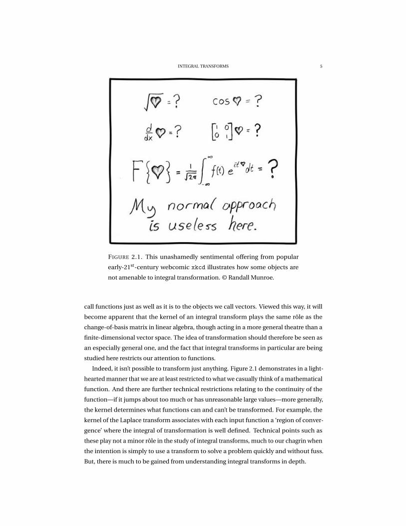
produces a continuous and periodic transform function. These four transform and their

properties are listed in Table 3.1 and represented concisely in Figure 3.2.


Continuous Discrete

Periodic DFT

Aperiodic FT

FS

-

�

DT FT

FIGURE 3.2. Diagrammatic representation of Table A.1, showing how

the various Fourier-type transforms act upon the properties of real-

space functions; the symmetries between each of the transforms being

more readily apparent in this form.

Partial Fourier Transforms (Segue). We can expand a little our conception of the Fourier

transform by way of a second pass at the geometric interpretation that was provided in

the chapter’s introduction. Each of the four different transforms presented in the previ-

ous section turn a variable (be it discrete or continuous) representing time or space into

a variable representing wavenumber or frequency; similarly, functions (be they periodic

or aperiodic) of one variable are transformed into functions of the other. Because both

the theory and practice of Fourier transforms have evolved with , it is common to speak

of the time and frequency domains, treating the transformation as a jump from one to

the other.

In fact, the Fourier transform of equation (3.2) can be generalised to a continuous

rotation through the time-frequency plane, that is, a conceptual plane in which an

axis representing time and an axis representing frequency are placed at right angles.

F corresponds to a rotation of π/2, taking a function purely of time to one purely of

freqeuncy, so that F 2 f =F{F

{f}}= f (−t ) and F 4 = 1. For any real angle θ, the partial

(or fractional) Fourier transform of a function f is

(3.15) F a {f}≡F

{f ;θ = a

π

2

}(ω) =

√1− i cotθ

2π

∫ ∞

−∞e

i2 [cotθ(ω2+t 2)−2cscθωt] f (t )d t .

The variables t and ω, though suggestive of time and frequency, are in fact meant to be

any general combination of the two. For example, a rotation of 45◦ =π/4 from the time

axis would be to a variable corresponding to an equal mix of frequency and time. In this

way, we can think of the integral Fourier operator as representing a rotation through this

somewhat unorthodox plane. Figure 3.3 shows one practical way in which the partial

transform can be used in signal processing.

Hermite Polynomials are Eigenfunctions of F . Encouraged by this development of the

Fourier transform into a rotation, we can, for the first time, begin to think properly about


FIGURE 3.3. A somewhat contrived example of the use of the partial

Fourier transform, for filtering noise that is a relatively simple function

of an unphysical variable representing a combination of time and fre-

quency. By using a partial Fourier transform, this noise can be excluded

using a pass filter in a single variable, before a counter-rotation renders

the cleaned signal back to the original domain; used within the GNU

Free Documentation License.

it as a (linear) operator. Linear operators are known to us mostly as matrices, where they

act on vectors to perform translations, rotations and reflections, or more generally, to

express the coördinates of a vector relative to a different set of axes; e.g.

(3.16)

[x ′

y ′

]=

[cosθ −sinθ

sinθ cosθ

][x

y

], or [v]C = [M ]B

C [v]B ;

where the former shows how a matrix acting as a linear operator rotates a vector in a

two-dimensional Euclidean space, while the latter, more generally, gives an equation by

which a vector in one coördinate frame (called a ‘basis’, a set of orthogonal, building-

block vectors like the axes on the Cartesian plane) is transformed to another. Shockingly,

the same equation holds with functions replacing vectors, and integral transforms (more

generally, integral operators) replacing the matrix that performs the basis change:

(3.17) f̃ =O { f },

where O = F would represent the Fourier transform. It is possible to go even further

and insist that the idea of a coördinate basis be carried over as well, so that the sin


and cos functions in the Fourier series represent the basis functions from which any

(periodic) function can be constructed. Indeed, it is quite easy to visualise this for

a low-dimensional case—each axis represents the contribution from a sinusoid of a

particular frequency, with each an and bn from equation (3.14) marking the location on

the corresponding axis. This idea can be extended to an infinite number of dimensions,

though it is more difficult to visualise.

What an integral transform really represents, then, is a change-of-basis between

different sets of orthogonal basis functions. Different transforms have different basis

functions, and this is represented by the kernel, which therefore captures the contribution

of each function in one basis set to each function in the other. This is perhaps the key

geometric point to be made about integral transforms9, and though it has been made

without rigour and precision, it is one that should be kept in your head and refined by

any future work with integral transform you might have.

All linear operators have a set of inputs (vectors or functions) that, when operated on,

return the same input multiplied by a scalar. In the context of matrices and linear algebra,

these are called eigenvectors and the scalars are called eigenvalues. That we should have

to think about eigen-anything when dealing with integral transforms might at first be a

surprise. But as we have discovered above, integral transforms of functions are analogous

to a change-of-basis for a vector. Remember that when we change the basis of a vector x,

the operation has an associated matrix A, and that this matrix will have associated with

it a set of vectors that are unaffected (up to stretching) by the change-of-basis.

So it goes with integral transforms, which to functions play the role that matrices

do to vectors. For an integral transform, there is a special set of functions that are

unchanged (up to multiplication by a scalar) when subject to that transform; these are

the eigenfunctions of the transform. In the case of the Fourier transform, there is no

unique set of eigenfunctions, but one set does commend itself more highly than others:

the Hermite functions (derived from the Hermite polynomials)

ψn(x) = 1√n!2n

pπ

e−x2/2Hn(x)(3.18)

= (−1)n√n!2n

pπ

ex2/2 d n

d xn e−x2,(3.19)

which, when acted on by the Fourier transform, give

(3.20) Fψn = (−i )nψn ;

in particular, the eigenvalue associated with each of the functions is (−i )n .

The Hermite functions arise in a vast number of physical contexts: they are the

stationary states of the Schrödinger equation with a square potential well, they are

9This is the climax of this lecture course, though there are plenty of interesting ideas still to come.


the shapelet functions used for decomposing gravitationally-lensed sources, they are

associated with the morphology of the cosmological density field, and so on.

Examples and Exercises. (to be added!)

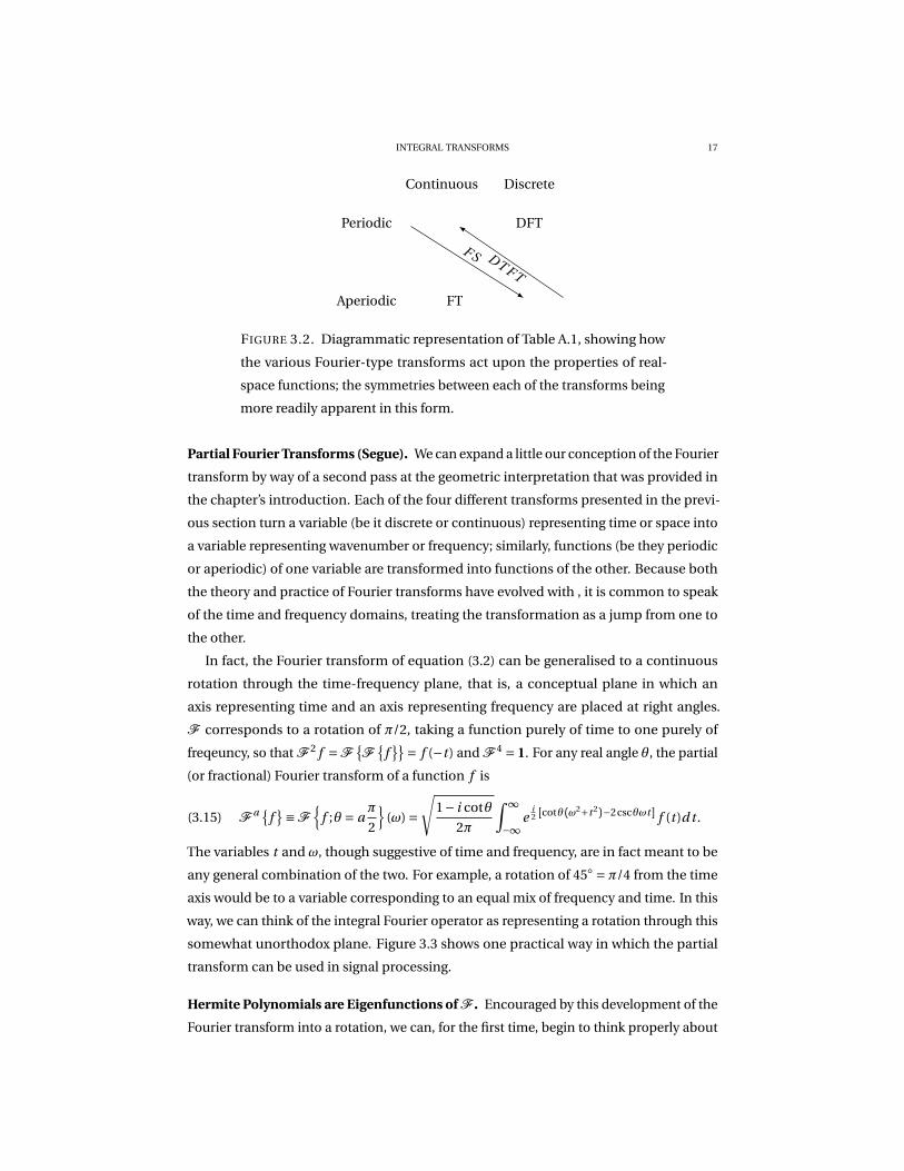
4. LAPLACE AND MELLIN TRANSFORMS

The transform carrying the name of the Marquis de Laplace is a cousin of the Fourier

transform and at first glance they are almost indistinguishable:

(4.1) L(s) =L{

f (x)}= ∫

f (x)e−st d x;

the difference is that s is complex rather than real (as k is), so that the exponent of the

kernel is in general a complex number rather than a pure imaginary one, as in the case of

i 2πkx. Of course, in the limit where s has no real component, identity with the Fourier

transform is obtained, modulo the factor 2π.

But this small change has profound consequences and the Laplace transform has very

different applications than those of F . Just as significantly, the issue of integration in

the complex plane introduces a number of subtle and important issues that should be

understood before throwing L around with aplomb. In this chapter, the properties of the

Laplace transform are established, before matters of convergence in the complex plane

are thrashed out. The latter paves the way for the introduction of the Mellin transform,

another cousin of F and L with exciting properties that regrettably have yet to find wide

application outside number theory.

Definition and Basic Theorems. The transform presented in equation (4.1) is known as

the two-sided Laplace transform. For reasons that will become apparent, integrating

from just from 0 to ∞—the one-sided transform—is often a useful approach. The inverse

of the two-sided transform is

(4.2) f (x) =L −1 {L(s)} = 1

2πi

∫ c+i∞

c−i∞F (s)e st d s,

though the conditions for existence are somewhat more stringent and convoluted than

for the Fourier transform. The reason for this is that the inverse must be integrated

throughout the complex plane (because the kernel is not either purely real or imaginary);

a discussion of contour integration and complex analysis would be required to explain

this in full. It will suffice to note that associated with each input function is a region in

which L and its inverse will converge; Table A.2, which gives a number of examples of

Laplace transform reults, also lists the values of the conjugate variable s for which the

inverse transform can be properly applied.

Most often, the region of convergence will be a strip in the complex plane of the form

α< Re s < β. We can see why it is the real part of s that is important by examining the


kernel of L −1, which is of the form e sx = e(Re s+i Im s)x . The imaginary part of s contributes

sinusoids—e±i kx , which are well-behaved—to the integrand, unlike the contributions

e± j x —corresponding to exponentials—which diverge toward ∞.

The values of α and β cannot be specified generally without a lot of exposition on

contour integration, but is worthwhile noting that α depends on the behaviour of the

right-hand side of the input function f (x > 0), and that β

The properties of the Laplace transform are, however, in almost direct correspondence

with those of F and are summarised in Table 4.1.


Th

eore

mf(

x)

L(s

)R

egio

no

fco

nve

rgen

ce

Sim

ilar

ity

f(a

x)

1 | a|L

( s a

)α<

Re

sa

<β

Ad

dit

ion

f 1(x

)+f 2

(x)

L1

(s)+

L2

(s)

max

(α1

,α2

)<R

es<

min

(β1

,β2

)

Shif

tf(

x−a

)e−

as L

(s)

α<

Re

s<β

Mo

du

lati

on

f(x

)co

sax

1 2[L

(s−i

a)+

L(s+i

a) ]

α<

Re

s<β

Co

nvo

luti

on

f 1(x

)∗f 2

(x)

L1

(s)L

2(s

)m

ax(α

1,α

2)<

Re

s<

min

(β1

,β2

)

Pro

du

ctf 1

(x)f

2(x

)1 2π

i

∫ c+i∞

c−i∞

L1

(a)L

2(s−a

)da

α1+α

2<

Re

s<β

1+β

2,

α1<

c<β

1

Au

toco

rrel

atio

nf(

x)∗

f(−x

)L

(s)L

(−s)

mo

dR

es<

min

(| α| ,∣ ∣ β∣ ∣ )

Dif

fere

nti

atio

nd

f(x

)d

xsL

(s)

α<

Re

s<β

Fin

ite

dif

fere

nce

f(x+a

/2)−

f(x−a

/2)

2si

nh

as 2

L(s

)α<

Re

s<β

Inte

grat

ion

∫ x −∞f(

u)d

uL

(s)

sm

ax(α

,0)<

Re

s<β

Rev

ersa

lf(−x

)L

(−s)

−β<

Re

s<−α

TA

BL

E4

.1.

Wri

tin

gth

e(t

wo

-sid

ed)

Lap

lace

tran

sfo

rmo

fage

ner

alfu

nct

ion

f(x

)as

L(s

)=L

{ f(x

)} ,th

enth

ep

rop

erti

eso

f

the

tran

sfo

rmca

nb

eex

pre

ssed

inth

efo

llow

ing

man

ner

;ad

apte

dfr

om

Bra

cew

ell,

R.N

.(19

78),

Th

eFo

uri

erTr

ansf

orm

and

Its

Ap

pli

cati

ons,

2nd

edit

ion

,McG

raw

-Hil

l.


Initial Value Problems (supplementary).

Enough Moments to Last a Lifetime. The Mellin transform and its applications to num-

ber theory (to be added!).

Examples and Exercises.

5. HANKEL, ABEL AND RADON TRANSFORMS

All three of the transforms in this chapter deal with the effects of projection and

symmetry on the integral transformation, and on the Fourier transform in particular.

Though little has been said about multi-dimensional problem to this point, the results of

Fourier analysis can be applied separately to orthogonal Cartesian axes ({x, y, z} in three

dimensions), with one integral and one conjugate variable for each (that is, {kx ,ky ,kz }).

Frequently one encounters problems in two- or three-dimensional space that symme-

try renders expressible by equations in less than two or three variables. Perhaps the most

common examples are spherical symmetry and axisymmetry. Writing the equations for

such systems in Cartesian coördinates fails to take advantage of the symmetry, which for

the two examples just given are a non-trivial mixture of x, y and z. Instead, by translating

to spherical polar coördinates {r,θ,φ} in the case of spherical symmetry, and cylindrical

polar coördinates {r,θ, z} in the case of axisymmetric problems, the properties of the

geometry in which the problems has been specified may allow us to discard one of the

variables, making the problem undoubtedly simpler.

Consider the example of the electric field outside a point charge such as an electron.

Because the field extending from the charge acts only in the radial direction, the variables

θ and φ are wholly unnecessary to give its full description; it is written Φ(r ) or ρ(r ) or

whatever. But think instead how one would write the same field in Cartesian coördinates.

Ugly!

So it goes with integral transforms and the Fourier transform especially. Because it is

so useful, it becomes desirable to apply F as widely as possible—but it is defined only

in terms of Cartesian coördinates and so may not make great use of any symmetries

inherent in the problem. Instead, it is possible to define the spherically (often written

‘circularly’, to emphasise the relatively low dimensionality) symmetric Fourier transform,

known as the Hankel transform H , in terms of a single variable r . In two dimensions

with spherical symmetry,

(5.1) f (x, y) = f (r ); where r 2 = x2 + y2;

when we define the Hankel transform in full momentarily, attention should be paid to its

relationship with F .


The other two transforms described in this chapter are no less useful than H . By

contrast though, they are useful in tandem with projection, which has some implicit and

intangible connection to symmetry that it is frequently best not to concern oneself with.

In the case of the Abel transform, which applies to a spherically symmetric distribution

projected onto a single radial axis, important information about both the full real- and

Fourier-space distributions can be extracted. The more general Radon transform, whose

real-word applications are multiplying more quickly than any other integral transform,

proceeds by calculating many slices through the function that is being transformed, with

the integral along each slice determining the value at a single point of the output function.

This process, of integrating along straight lines, is used extensively in medical physics,

such as MRI scanning and CAT (tomography).

Symmetry, projection and integral transformation come together in the FH A cy-

cle and its generalisation, known as the projection-slice theorem. This topic, and the

subsequent denouement, bring the course to a close.

Definitions and Basic Theorems. The Hankel transform and its inverse are

Hν(k) =H{

f (r )} =

∫ ∞

0f (r )Jν(kr )r dr(5.2)

f (r ) =H −1 {Hν(k)} =∫ ∞

0Hν(k)Jν(kr )dk;(5.3)

note that, unlike the Fourier, Laplace and Mellin transforms, H is its own inverse. The

function Jν is a Bessel function10 of the first kind:

(5.4) Jν(x) =∞∑

n=0

(−1)n

n!Γ(n +ν+1)

( x

2

)2n+ν;

the quantity ν≥ 0, is referred to as the order of the Bessel function and equivalently as

the order of the Hankel transform.

The Hankel transform amounts to a Fourier transform along the circular axis of

symmetry of the two-dimensional function,viz.∫ ∞

−∞

∫ ∞

−∞f (x, y)e−2π(xkx+yky )d x d y =

∫ ∞

0

∫ 2π

0f (r )e−i 2πqr cos(θ−φ)r dr dθ

=∫ ∞

0f (r )

[∫ 2π

0e−i 2πqr cosθdθ

]r dr

= 2π∫ ∞

0f (r )J0(2πqr )r dr,

10Bessel functions play a proportionally smaller rôle in astronomy today than they once did, which can

only be a shame, and contributes to a certain clunky inability to work with them among those of the author’s

generation. It is important to grasp that they are intrinsically no more complicated than the trigonometric

sin and cos function, and that all can be viewed as closed-form solutions to particular second-order ordinary

differential equations.


FIGURE 5.1. The protagonists of this chapter: Hermann Hankel (top-

left), Johann Radon (top-right) and valuable Norwegian currency bear-

ing the portrait of Niels Henrik Abel (bottom).

where (x, y) has been mapped to (r,θ) and (kx ,ky ) to (q,φ); a key relation for the Bessel

function of order zero,

(5.5) J0(z) = 1

2π

∫ 2π

0e−i z cosθdθ,

has also been used.


Just as the Fourier transform changes the functional basis of an input function f to

that of trigonometric sin and cos functions, the Hankel transform rebuilds f out of Bessel

functions. This can be seen in the discrete case (analogous to the Fourier series, and

cheekily called the Fourier–Bessel, rather than Bessel–Fourier, series):

(5.6) f (x) =∞∑

n=0cn Jν

(λn x

b

),

where λn and b, both particular parameters of the Bessel function, play the rôle of the

factor of nπ/2 in the Fourier series. Of course, the coëfficients cn are calculated in just

the same way as Fourier originally suggested, using the Bessel functions rather than

cos(xnπ/2) in the integrand. Once again, this works because the Bessel functions are a

set of orthogonal basis functions; there are many other sets of such functions available,

those the Fourier and Fourier–Bessel series tend to be the most widely used.

The Abel transform is defined to be

(5.7) A(y) =A{

f (r )}= 2

∫ ∞

y

f (r )r dr√r 2 − y2

,

and, when the function declines more quickly that the inverse of r , the inverse Abel

transform exists as well:

(5.8) f (r ) =A −1 {F (y)

}=− 1

π

∫ ∞

r

dF

d y

d y√y2 − r 2

.

This transform has the effect of projecting the circularly symmetric function f (r ) onto a

single Cartesian axis; on the face of it, it may appear that information is being tossed away,

but it must be remembered that the original function is really only one-dimensional

because of the symmetry. The Abel transforms changes the radial axis of symmetry into

a Cartesian axis of projection; this process has many applications in imaging (e.g. in

cathode-ray tube television sets).

The Radon transform is a generalisation of the Abel transformation to projection

through arbitrary coördinates and for this reason has a peculiarly general-looking kernel,

which is defined parametrically. The idea is to integrate the function along a series of

straight lines

(5.9) `(α, s) :

[x(t )

y(t )

]=

[sinα cosα

−cosα sinα

][t

s

],

so that

R(α, s) =R{

f (x, y)}= ∫ ∞

−∞f(x(t ), y(t )

)d t ,(5.10)

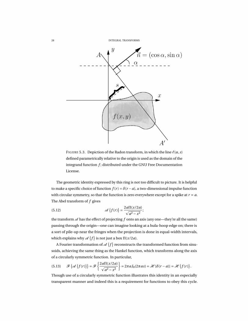
is the Radon transform of f (x, y). It is as though the function f has been shot through

with lines from every direction and displacement, with the integral of the function along

a single corresponding to the value of the Radon transform at the position specified by

the parameters that define the line. Figure 5.3 shows how the values α and s define a line


FIGURE 5.2. The Abel transform places a circularly symmetric function

in projection along straight lines; in the figure, an observed measures a

single value of A{

f}

by integrating f (r ) along their (Cartesian) line-of-

sight at a fixed height above the x-axis. Doing so for all heights gives

the Abel transform of f .

along which the function is integrated: it bears repeating that the Radon transform is the

integral along every such line; as there are as many lines through the plane as points in it

(!), R(α, s) is of course also a two-dimensional function.

FA =H . A remarkable identity exists between the Fourier, Abel and Hankel transforms

that is aptly summarised by the equation

(5.11) FA { f } =H { f }

. The application of an Abel transform, followed by a Fourier transform (in that order,

mind) is equivalent to the application of a Hankel transform. Equivalently, because

the Hankel transform is its own inverse (H −1 = H and H −1H = 1), we can write

equation (5.11) as H FA = 1, so that the three transforms are ordered in a ring that takes

a function right back to where it started when after successive application.


FIGURE 5.3. Depiction of the Radon transform, in which the line `(α, s)

defined parametrically relative to the origin is used as the domain of the

integrand function f ; distributed under the GNU Free Documentation

License.

The geometric identity expressed by this ring is not too difficult to picture. It is helpful

to make a specific choice of function f (r ) = δ(r −a), a two-dimensional impulse function

with circular symmetry, so that the function is zero everywhere except for a spike at r = a.

The Abel transform of f gives

(5.12) A{

f (r )}= 2aΠ(x/2a)p

a2 −x2;

the transform A has the effect of projecting f onto an axis (any one—they’re all the same)

passing through the origin—one can imagine looking at a hula-hoop edge on; there is

a sort of pile-up near the fringes when the projection is done in equal-width intervals,

which explains why A{

f}

is not just a box Π(x/2a).

A Fourier transformation of A{

f}

reconstructs the transformed function from sinu-

soids, achieving the same thing as the Hankel function, which transforms along the axis

of a circularly symmetric function. In particular,

(5.13) F{A

{f (r )

}}=F

{2aΠ(x/2a)p

a2 −x2

}= 2πa J0(2πas) =H {δ(r −a)} =H

{f (r )

}.

Though use of a circularly symmetric function illustrates this identity in an especially

transparent manner and indeed this is a requirement for functions to obey this cycle.


FIGURE 5.4

This is because the Abel transform projects a function in just the way that the Hankel

transform requires just when that function is circularly-symmetric; a sensible way to

view the identity is as a factorisation of the Hankel transform into two distinct phases:

the projection, and then the transformation to frequency space.

Projection–slice theorem. The result of the previous section is part of more general re-

lationship between projection and the Fourier transform. In two- and three-dimensional

spaces, it is not too hard to see how the result FA =H might be interpreted in a much

more general fashion. The projection–slice theorem asserts the equivalence of projection

in real space and slicing in Fourier space. A more descriptive statement is that the Fourier

transform of a projected function is equivalent to a slice through the Fourier transform

of the unprojected function. Figure 5.4 illustrates this process, which might by written in

symbols as

(5.14) F{P { f (x)}

}= S{F

{f (x)

}},

where P and S are operators representing the geometric actions of projection onto an

axis and slicing in a straight line through a function. Significantly, the direction of the

slice in Fourier space must be the same as the direction of the projection in real space

(that is, orthogonal to the axis onto which the function is projected).

Theorem 5.1. [Projection–slice theorem] In n-dimensions, let f (r) be an n-dimensional

function that is projected along m < n orthogonal dimensions to give the (n−m)-dimensional

projected function p f (r). Then, F{

p f (r)}

is a series of m slices through through F{

f (r)}

,

where the each slice direction is parallel to its corresponding real-space direction of projec-

tion.

Proof. We prove just the case n = 3, though generalisation is straight-forward. Let

f (x, y, z) be a three dimensional function that is, without loss of generality, projected


along the y- and z-axes, giving

(5.15) p(x) ≡∫ ∞

−∞

∫ ∞

−∞f (x, y, z)d y d z.

Then, writing F3 for the three-dimensional Fourier transform and S for the operation of

slicing,

F (kx ,ky ,kz ) = F3{ f (x, y, z)} =∫ ∞

−∞

∫ ∞

−∞

∫ ∞

−∞f (x, y, z)e−i 2π(xkx+yky )d x d y d z

⇒ s(kx ) ≡ S(

f (kx ,ky ,kz ))

= F (kx ,0,0)

=∫ ∞

−∞

∫ ∞

−∞

∫ ∞

−∞f (x, y, z)e−i 2πxkx d x d y d z

=∫ ∞

−∞

[∫ ∞

−∞

∫ ∞

−∞f (x, y, z)d y d z

]e−i 2πxkx d x

=∫ ∞

−∞p(x)e−i 2πxkx d x

= F{

p(x)}

.

�

Unlike the FH A cycle demonstrated in the previous section, this result is perfectly

general for all input functions f . This theorem finds a wide variety of applications in

the science, engineering and medicine. The process of tomographic back-projection

consists of first measuring a (say, two-dimensional) function f (x, y) projected along a

series of angles, then, transforming the measurement into Fourier space, interpolating

over the slices that Theorem 5.1 tells us have been measured. This gives a reconstruction

of the Fourier transform of the full function, so that when the inverse Fourier transform

is taken, (an albeit degraded version of) the full f (x, y) is found. Ideally, the projections

are made at equally-space angles; taking more and more projections will include higher

and higher frequency information into the final signal, and in practice this process can

be done efficiently.

An example from cosmology is the calculation of the three-dimensional power spec-

trum from the projected two-point correlation. This has proved to be of great utility in the

study of cosmological structure; while the angular position of galaxies can be measured

very precisely, their distance as determined by redshift is substantially more expensive

to obtain. Consequently, the two-point correlation function, a count of the distances

between pairs of objects as a function of r , is more accurately estimated in projection

along the radial axis.

In the 1950s, Limber devised a method by which to reconstruct the spatial correlation

function by using an inverse Abel transform, under the assumption of spherical symmetry.

This assumption is justified, particularly on large scales, by the homogeneity and isotropy


of the Universe. Equivalently, we can think of this as treating the single slice in Fourier

space measured by the projected correlation function as representative of the full Fourier

space distribution; the power spectrum and the two-point correlation function are a

Fourier transform pair, so the projected correlation function gives access, via either the

inverse Abel transform or the projection–slice theorem, to the full three-dimensional

power spectrum of the Universe.

Examples and Exercises.

·FINIS·


APPENDIX A. REFERENCE TABLE OF TRANSFORMS

Table A.1: Table of Fourier transforms.

f (x) F (k) = ∫ ∞−∞ f (x)e−i 2πkx d x Notes

1 δ(k)1x −iπsgnk1

a2+x2e−a|k|

a Re a > 0x

a2+x2 − i2

ke−a|k|a Re a > 0

e i ax δ(k +a)

e−i a|x| 1π

aa2+k2

xe−i a|x| 1π

2ai k

(a2+k2)2

|x|e−i a|x| 1π

a2−k2

(a2+k2)2

e−ax2√

πa e−(πk)2/a

Π(ax) =

0 if |x| > 1

2a12 if |x| = 1

2a

1 if |x| < 12a

1|a|

sin(πk/a)πk/a

Table A.2: Table of Laplace transforms L{

f (x)}= ∫ ∞

−∞ f (x)e−sx d x.

f (x) L(s) Convergence

δ(x) 1

H(x) 1s 0 < Re s

xH(x) 1s2 0 < Re s

xe−ax H(x) 1(s+a)2 −Re a < Re s

(1−e−ax )H(x) as(s+a) max(0,−Re a) < Re s

cos axH(x) ss2+a2 0 < Re s

sin axH(x) as2+a2 0 < Re s

e−a|x| 2aa2−s2 −Re a < Re s < Re a


Table A.3: Table of Mellin transforms.

f (x) M(s) = ∫ ∞−∞ f (x)xs−1d s Notes

δ(x −a) as−1

H(x −a) − as

s

xn H(x −a) − as+ns+n

e−ax a−sΓ(s) Re a, s > 0

e−ax2 12as/2 Γ( s

2 )

sin(ax) a−sΓ(s)sin πs2 −1 < Re s < 1

cos(ax) a−sΓ(s)cos πs2 0 < Re s < 1

11+x πcscπs

11−x πcotπs

1(1+x)a

Γ(s)Γ(a−s)Γ(a) Re a > 0

11+x2

π2 csc πs

2

(1−x)a−1H(1−x) Γ(s)Γ(a)Γ(s+a) Re a > 0

(x −1)a H(x −1) Γ(a−s)Γ(1−a)Γ(1−s) 0 < Re a < 1

log(1+x) πs cscπs −1 < Re s < 0

π2 −arctan x π

2s sec s2

Λ(x −1) ={

0 if |x −1| ≥ 1

1−|x −1| if |x −1| < 1

{2(2s−1)s(s+1) if s 6= 0

2log2 if s = 0Re s >−1

Hankel Transforms.

Abel Transforms.

Radon Transforms.

Documents

Integral Transforms for You & Me Royal Observatory ... · Integral Transforms for You & Me Royal Observatory Edinburgh Institute for Astronomy J. Berian James March 2008. CONTENTS