Chapter 3

Integral Transforms

This part of the course introduces two extremely powerful methods to solvingdifferential equations: the Fourier and the Laplace transforms. Beside itspractical use, the Fourier transform is also of fundamental importance inquantum mechanics, providing the correspondence between the position andmomentum representations of the Heisenberg commutation relations.

An integral transform is useful if it allows one to turn a complicatedproblem into a simpler one. The transforms we will be studying in this partof the course are mostly useful to solve differential and, to a lesser extent,integral equations. The idea behind a transform is very simple. To be definitesuppose that we want to solve a differential equation, with unknown functionf . One first applies the transform to the differential equation to turn it intoan equation one can solve easily: often an algebraic equation for the transformF of f . One then solves this equation for F and finally applies the inversetransform to find f . This circle (or square!) of ideas can be representeddiagrammatically as follows:

differential equation for f

algebraic equation for F solution: F

solution: f

transforminverse

transform

6

?

-

-

We would like to follow the dashed line, but this is often very difficult.

185

Therefore we follow the solid line instead: it may seem a longer path, but ithas the advantage of being straightforward. After all, what is the purpose ofdeveloping formalism if not to reduce the solution of complicated problemsto a set of simple rules which even a machine could follow?

We will start by reviewing Fourier series in the context of one particularexample: the vibrating string. This will have the added benefit of introduc-ing the method of separation of variables in order to solve partial differentialequations. In the limit as the vibrating string becomes infinitely long, theFourier series naturally gives rise to the Fourier integral transform, which wewill apply to find steady-state solutions to differential equations. In partic-ular we will apply this to the one-dimensional wave equation. In order todeal with transient solutions of differential equations, we will introduce theLaplace transform. This will then be applied, among other problems, to thesolution of initial value problems.

3.1 Fourier series

In this section we will discuss the Fourier expansion of periodic functions ofa real variable. As a practical application, we start with the study of thevibrating string, where the Fourier series makes a natural appearance.

3.1.1 The vibrating string

Consider a string of length L which is clamped at both ends. Let x denotethe position along the string: such that the two ends of the string are atx = 0 and x = L, respectively. The string has tension T and a uniformmass density µ, and it is allowed to vibrate. If we think of the string asbeing composed of an infinite number of infinitesimal masses, we model thevibrations by a function ψ(x, t) which describes the vertical displacement attime t of the mass at position x. It can be shown that for small verticaldisplacements, ψ(x, t) obeys the following equation:

T∂2ψ(x, t)

∂x2= µ

∂2ψ(x, t)

∂t2,

which can be recognised as the one-dimensional wave equation

∂2

∂x2ψ(x, t) =

1

c2

∂2

∂t2ψ(x, t) , (3.1)

where c =√

T/µ is the wave velocity. This is a partial differential equationwhich needs for its solution to be supplemented by boundary conditions for

186

x and initial conditions for t. Because the string is clamped at both ends,the boundary conditions are

ψ(0, t) = ψ(L, t) = 0 , for all t. (3.2)

As initial conditions we specify that at t = 0,

∂ψ(x, t)

∂t

∣∣∣∣t=0

= 0 and ψ(x, 0) = f(x) , for all x, (3.3)

where f is a continuous function which, for consistency with the boundaryconditions (3.2), must satisfy f(0) = f(L) = 0. In other words, the string isreleased from rest from an initial shape given by the function f .

This is not the only type of initial conditions that could be imposed. For example, in thecase of, say, a piano string, it would be much more sensible to consider an initial conditionin which the string is horizontal so that ψ(x, 0) = 0, but such that it is given a blow at

t = 0, which means that∂ψ(x,t)

∂t|t=0 = g(x) for some function g. More generally still, we

could consider mixed initial conditions in which ψ(x, 0) = f(x) and∂ψ(x,t)

∂t|t=0 = g(x).

These different initial conditions can be analysed in roughly the same way.

We will solve the wave equation by the method of separation of variables.This consists of choosing as an Ansatz for ψ(x, t) the product of two functions,one depending only on x and the other only on t: ψ(x, t) = u(x) v(t). Wedo not actually expect the solution to be of this form; but because, as wewill review below, the equation is linear and one can use the principle ofsuperposition to construct the desired solution out of decomposable solutionsof this type. At any rate, inserting this Ansatz into (3.1), we have

u′′(x) v(t) =1

c2u(x)v′′(t) ,

where we are using primes to denote derivatives with respect to the variableon which the function depends: u′(x) = du/dx and v′(t) = dv/dt. We nowdivide both sides of the equation by u(x) v(t), and obtain

u′′(x)

u(x)=

1

c2

v′′(t)v(t)

.

Now comes the reason that this method works, so pay close attention.Notice that the right-hand side does not depend on x, and that the left-handside does not depend on t. Since they are equal, both sides have to be equalto a constant which, with some foresight, we choose to call −λ2, as it will bea negative number in the case of interest. The equation therefore breaks upinto two ordinary differential equations:

u′′(x) = −λ2 u(x) and v′′(t) = −λ2 c2 v(t) .

187

The boundary conditions say that u(0) = u(L) = 0.Let us consider the first equation. It has three types of solutions depend-

ing on whether λ is nonzero real, nonzero imaginary or zero. (Notice that−λ2 has to be real, so that these are the only possibilities.) If λ = 0, thenthe solution is u(x) = a + b x. The boundary condition u(0) = 0 means thata = 0, but the boundary condition u(L) = 0 then means that b = 0, whenceu(x) = 0 for all x. Clearly this is a very uninteresting solution. Let usconsider λ imaginary. Then the solution is now a exp(|λ|x) + b exp(−|λ|x).Again the boundary conditions force a = b = 0. Therefore we are left withthe possibility of λ real. Then the solution is

u(x) = a cos λx + b sin λx .

The boundary condition u(0) = 0 forces a = 0. Finally the boundary condi-tion u(L) = 0 implies that

sin λL = 0 =⇒ λ =nπ

Lfor n an integer.

Actually n = 0 is an uninteresting solution, and because of the fact that thesine is an odd function, negative values of n give rise to the same solution(up to a sign) as positive values of n. In other words, all nontrivial distinctsolution are given (up to a constant multiple) by

un(x) ≡ sin λn x , with λn =nπ

Land where n = 1, 2, 3, · · · . (3.4)

Let us now solve for v(t). Its equation is

v′′(t) = −λ2c2v(t) ,

whencev(t) = a cos λct + b sin λct .

The first of the two initial conditions (3.3) says that v′(0) = 0 whence b = 0.Therefore for any positive integer n, the function

ψn(x, t) = sin λnx cos λnct , with λn =nπ

L,

satisfies the wave equation (3.1) subject to the boundary conditions (3.2)and to the first of the initial conditions (3.3).

Now notice something important: the wave equation (3.1) is linear; thatis, if ψ(x, t) and φ(x, t) are solutions of the wave equation, so is any linearcombination α ψ(x, t) + β φ(x, t) where α and β are constants.

188

Clearly then, any linear combination of the ψn(x, t) will also be a so-lution. In other words, the most general solution subject to the boundaryconditions (3.2) and the first of the initial conditions in (3.3) is given by alinear combination

ψ(x, t) =∞∑

n=1

bn sin λnx cos λnct .

Of course, this expression is formal as it stands: it is an infinite sum whichdoes not necessarily make sense, unless we chose the coefficients bn in sucha way that the series converges, and that the convergence is such that we candifferentiate the series termwise at least twice.

We can now finally impose the second of the initial conditions (3.3):

ψ(x, 0) =∞∑

n=1

bn sin λnx = f(x) . (3.5)

At first sight this seems hopeless: can any function f(x) be represented asa series of this form? The Bernoullis, who were the first to get this far,thought that this was not the case and that in some sense the solution wasonly valid for special kinds of functions for which such a series expansion ispossible. It took Euler to realise that, in a certain sense, all functions f(x)with f(0) = f(L) = 0, can be expanded in this way. He did this by showinghow the coefficients bn are determined by the function f(x).

To do so let us argue as follows. Let n and m be positive integers andconsider the functions un(x) and um(x) defined in (3.4). These functionssatisfy the differential equations:

u′′n(x) = −λ2n un(x) and u′′m(x) = −λ2

m um(x) .

Let us multiply the first equation by um(x) and the second equation by un(x)and subtract one from the other to obtain

u′′n(x) um(x)− un(x) u′′m(x) = (λ2m − λ2

n) un(x) um(x) .

We notice that the left-hand side of the equation is a total derivative

u′′n(x) um(x)− un(x) u′′m(x) = (u′n(x) um(x)− un(x) u′m(x))′

,

whence integrating both sides of the equation from x = 0 to x = L, we obtain

(λ2m − λ2

n)

∫ L

0

um(x) un(x) dx = (u′n(x) um(x)− un(x) u′m(x))∣∣∣L

0= 0 ,

189

since un(0) = un(L) = 0 and the same for um. Therefore we see that unlessλ2

n = λ2m, which is equivalent to n = m (since n, m are positive integers), the

integral∫ L

0um(x) un(x) dx vanishes. On the other hand, if m = n, we have

that∫ L

0

un(x)2 dx =

∫ L

0

(sin

nπx

L

)2

dx =

∫ L

0

(1

2− 1

2cos

2nπx

L

)dx =

L

2.

Therefore, in summary, we have the orthogonality property of the functionsum(x): ∫ L

0

um(x) un(x) dx =

L2

, if n = m, and

0 , otherwise.(3.6)

Let us now go back to the solution of the remaining initial condition (3.5).This condition can be rewritten as

f(x) =∞∑

n=1

bn un(x) =∞∑

n=1

bn sinnπx

L. (3.7)

Let us multiply both sides by um(x) and integrate from x = 0 to x = L:

∫ L

0

f(x) um(x) dx =∞∑

n=1

bn

∫ L

0

un(x) um(x) dx ,

where we have interchanged the order of integration and summation withimpunity.1 Using the orthogonality relation (3.6) we see that of all the termsin the right-hand side, only the term with n = m contributes to the sum,whence ∫ L

0

f(x) um(x) dx = bmL

2,

or in other words,

bm =2

L

∫ L

0

f(x) um(x) dx , (3.8)

a formula due to Euler. Finally, the solution of the wave equation (3.1) withboundary conditions (3.2) and initial conditions (3.3) is

ψ(x, t) =∞∑

n=1

bn sinnπx

Lcos

nπct

L, (3.9)

1This would have to be justified, but in this part of the course we will be much morecavalier about these things. The amount of material that would have to be introduced tobe able to justify this procedure is too much for a course at this level and of this length.

190

where

bn =2

L

∫ L

0

f(x) sinnπx

Ldx .

Inserting this expression into the solution (3.9), we find that

ψ(x, t) =∞∑

n=1

[2

L

∫ L

0

f(y) sinnπy

Ldy

]sin

nπx

Lcos

nπct

L

=

∫ L

0

[2

L

∞∑n=1

sinnπy

Lsin

nπx

Lcos

nπct

L

]f(y) dy

=

∫ L

0

K(x, y; t) f(y) dy ,

where the propagator K(x, y, t) is (formally) defined by

K(x, y; t) ≡∞∑

n=1

2

Lsin

nπy

Lsin

nπx

Lcos

nπct

L.

To understand why it is called a propagator, notice that

ψ(x, t) =

∫ L

0

K(x, y; t) ψ(y, 0) dy ,

so that one can obtain ψ(x, t) from its value at t = 0 simply by multiplyingby K(x, y; t) and integrating; hence K(x, y; t) allows us to propagate theconfiguration at t = 0 to any other time t.

Actually, the attentive reader will have noticed that we never showed thatthe series

∑∞n=1 bnun(x), with bn given by the Euler formula (3.8) converges

to f(x). In fact, it is possible to show that it does, but the convergence is notnecessarily pointwise (and certainly not uniform). We state without proofthe following result:

limN→∞

∫ L

0

(f(x)−

N∑n=1

bn un(x)

)2

dx = 0 . (3.10)

In other words, the function

h(x) ≡ f(x)−∞∑

n=1

bn un(x)

has the property that the integral∫ L

0

h(x)2 dx = 0 .

191

This however does not mean that h(x) = 0, but only that it is zero almosteverywhere.

To understand this notice consider the (discontinuous) function

h(x) =

(1 , for x = x0, and

0 , otherwise.

Then it is clear that the improper integral

Z L

0h(x)2 dx = lim

r,s0

Z x0−r

0+

Z L

x0+s

h(x)2 dx = 0 .

The same would happen if h(x) were zero but at a finite number of points.

Of course, if h(x) were continuous and zero almost everywhere, it wouldhave to be identically zero. In this case the convergence of the series (3.7)would be pointwise. This is the case if f(x) is itself continuous.

Expanding (3.10), we find that

∫ L

0

f(x)2 dx− 2∞∑

n=1

bn

∫ L

0

f(x) un(x) dx

+∞∑

n,m=1

bn bm

∫ L

0

un(x) um(x) dx = 0 .

Using (3.8) and (3.6) we can simplify this a little

∫ L

0

f(x)2 dx− 2∞∑

n=1

L

2b2n +

∞∑n=1

L

2b2n = 0 ,

whence ∞∑n=1

b2n =

2

L

∫ L

0

f(x)2 dx .

Since f(x)2 is continuous, it is integrable, and hence the right-hand side isfinite, whence the series

∑∞n=1 b2

n also converges. In particular, it means thatlimn→∞ bn = 0.

3.1.2 The Fourier series of a periodic function

We have seen above that a continuous function f(x) defined on the interval[0, L] and vanishing at the boundary, f(0) = f(L) = 0, can be expanded interms of the functions un(x) = sin(nπx/L). In this section we will generalisethis and consider similar expansions for periodic functions.

192

To be precise let f(x) be a complex-valued function of a real variablewhich is periodic with period L: f(x + L) = f(x) for all x. Periodicitymeans that f(x) is uniquely determined by its behaviour within a period. Inother words, if we know f in the interval [0, L] then we know f(x) everywhere.Said differently, any function defined on [0, L], obeying f(0) = f(L) can beextended to the whole real line as a periodic function. More generally, theinterval [0, L] can be substituted by any one period [x0, x0 + L], for some x0

with the property that f(x0) = f(x0+L). This is not a useless generalisation:it will be important when we discuss the case of f(x) being a discontinuousfunction. The strength of the Fourier expansion is that it treats discontinuousfunctions (at least those with a finite number of discontinuities in any oneperiod) as easily as it treats continuous functions. The reason is, as we statedbriefly above, that the convergence of the series is not pointwise but ratherin the sense (3.10), which simply means that it converges pointwise almosteverywhere.

The functions en(x) ≡ exp(i2πnx/L) are periodic with period L, sinceen(x + L) = en(x) exp(i2πn) = en(x). Therefore we could try to expand

f(x) =∞∑

n=−∞cn en(x) , (3.11)

for some complex coefficients cn. This series is known as a trigonometricof Fourier series of the periodic function f , and the cn are called theFourier coefficients. Under complex conjugation, the exponentials en(x)satisfy en(x)∗ = e−n(x), and also the following orthogonality property:

∫ L

0

em(x)∗ en(x) dx =

∫ L

0

ei2π(n−m)x/L dx =

L , if n = m, and

0 , otherwise.

Therefore if we multiply both sides of (3.11) by em(x)∗ and integrate, we findthe following formula for the Fourier coefficients:

cm =1

L

∫ L

0

em(x)∗ f(x) dx .

It is important to realise that the exponential functions en(x) satisfy theorthogonality relation for any one period, not necessarily [0, L]:

∫

oneperiod

em(x)∗ en(x) dx =

L , if n = m, and

0 , otherwise;(3.12)

193

whence the Fourier coefficients can be obtained by integrating over any oneperiod:

cm =1

L

∫

oneperiod

em(x)∗ f(x) dx . (3.13)

Again we can state without proof that the series converges pointwisealmost everywhere within any one period, in the sense that

limN→∞

∫

oneperiod

∣∣∣∣∣f(x)−N∑

n=−N

cn en(x)

∣∣∣∣∣

2

dx = 0 ,

whenever the cn are given by (3.13).

There is one special case where the series converges pointwise and uniformly. Let g(z) bea function which is analytic in an open annulus containing the unit circle |z| = 1. We sawin Section 2.3.4 that such a function is approximated uniformly by a Laurent series of theform

g(z) =∞X

n=−∞bn zn ,

where the bn are given by equations (2.53) and (2.54). Evaluating this on the unit circlez = eiθ, we have that

g(eiθ) =∞X

n=−∞bn einθ , (3.14)

and the coefficients bn are given by

bn =1

2π

Z 2π

0g(eiθ) e−inθ dθ , (3.15)

which agrees precisely with the Fourier series of the function g(eiθ) which is periodic withperiod 2π. We can rescale this by defining θ = 2πx/L where x is periodic with period L.Let f(x) ≡ g(exp(i2πx/L)), which is now periodic with period L. Then the Laurent series(3.14) becomes the Fourier series (3.11) where the Laurent coefficients (3.15) are now giveby the Fourier coefficients (3.13).

Some examples

1

ππ

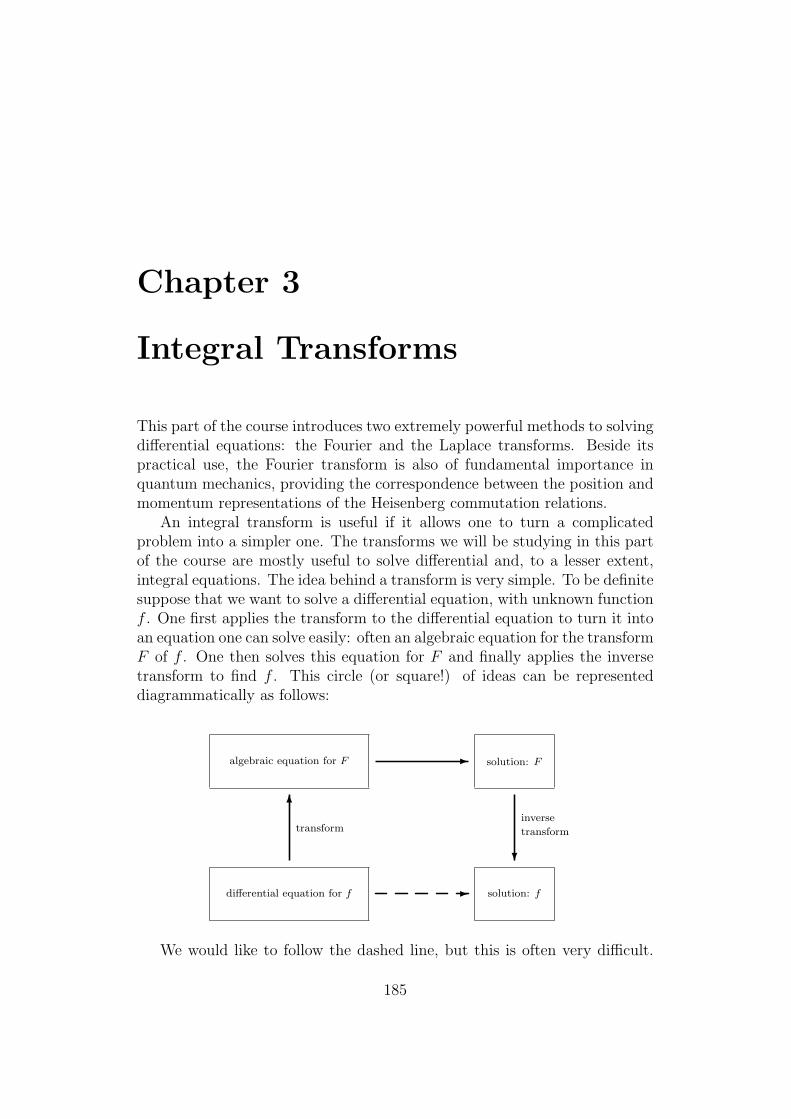
Figure 3.1: Plot of | sin x| for x ∈ [−π, π].

194

Let us now compute some examples of Fourier series. The first example isthe function f(x) = | sin x|. A graph of this function shows that it is periodicwith period π, as seen in Figure 3.1. We therefore try an expansion of theform

| sin x| =∞∑

n=−∞cn ei2nx ,

where the coefficients cn are given by

cn =1

π

∫ π

0

| sin x| e−i2nx dx =1

π

∫ π

0

sin x e−i2nx dx .

We can expand sin x into exponentials to obtain

cn =1

2πi

∫ π

0

(eix − e−ix

)e−i2nx dx

=1

2πi

[∫ π

0

e−i(2n−1)x dx−∫ π

0

e−i(2n+1)x dx

]

=1

2πi

[i

2n− 1

(e−i(2n−1)π − 1

)− i

2n + 1

(e−i(2n+1)π − 1

)]

=1

2πi(−2i)

[1

2n− 1− 1

2n + 1

]

= − 2

π

1

4n2 − 1.

Therefore,

| sin x| =∞∑

n=−∞− 2

π

1

4n2 − 1ei2nx =

2

π−

∞∑n=1

4

π

1

4n2 − 1cos 2nx .

Notice that this can be used in order to compute infinite sums. Evaluatingthis at x = 0, we have that

∞∑n=1

1

4n2 − 1= 1

2,

whereas evaluating this at x = π/2, we have that

∞∑n=1

(−1)n

4n2 − 1=

2− π

4.

Of course, we could have summed these series using the residue theorem, asexplained in Section 2.4.5.

195

1

−1

−2π

−π π

2π

Figure 3.2: Plot of f(x) for x ∈ [−2π, 2π].

As a second example, let us consider the function f(x) defined in theinterval [−π, π] by

f(x) =

−1− 2

πx , if −π ≤ x ≤ 0, and

−1 + 2π

x , if 0 ≤ x ≤ π.(3.16)

and extended periodically to the whole real line. A plot of this function forx ∈ [−2π, 2π] is shown in Figure 3.2. It is clear from the picture that f(x)has periodicity 2π, whence we expect a Fourier series of the form

f(x) =∞∑

n=−∞cn einx ,

where the coefficients are given by

cn =1

2π

∫ π

−π

f(x) e−inx dx

=1

2π

[∫ 0

−π

(−1− 2

πx) e−inx dx +

∫ π

0

(−1 +2

πx) e−inx dx

]

=1

2π

∫ π

0

(−1 +2

πx)

[einx + e−inx

]dx

= − 1

π

∫ π

0

cos(nx) dx +2

π2

∫ π

0

x cos(nx) dx .

We must distinguish between n = 0 and n 6= 0. Performing the elementaryintegrals for both of these cases, we arrive at

cn =

2

π2 n2 [(−1)n − 1] , for n 6= 0, and

0 , for n = 0.(3.17)

196

Therefore we have that

f(x) =∞∑

n=−∞n 6=0

2

π2 n2[(−1)n − 1] einx

=∞∑

n=1

4

π2 n2[(−1)n − 1] cos nx

=∞∑

n=1n odd

− 8

π2 n2cos nx

=∞∑

`=0

8

π2

−1

(2` + 1)2cos(2` + 1) x .

1

−1

−3π −2π

−π π 2π

3π

Figure 3.3: Plot of g(x) for x ∈ [−3π, 3π].

Finally we consider the case of a discontinuous function:

g(x) =x

π, where x ∈ [−π, π],

and extended periodically to the whole real line. The function has period2π, and so we expect a series expansion of the form

g(x) =∞∑

n=−∞cn einx ,

where the Fourier coefficients are given by

cn =1

2π

∫ π

−π

g(x) e−inx dx

=1

2π2

∫ π

−π

x e−inx dx .

197

We must distinguish the cases n = 0 and n 6= 0. In either case we canperform the elementary integrals to arrive at

cn =

0 , if n = 0,

iπ n

(−1)n , otherwise.

Therefore,

g(x) =∞∑

n=−∞n6=0

i

π n(−1)neinx =

∞∑n=1

−2

π n(−1)n sin n x .

Now notice something curious: the function g(x) is discontinuous at x = (2`+1)π. Evaluating the series at such values of x we see that because sin n(2` +1)π = 0, the series sums to zero for these values. In other words, g(x) isonly equal to the Fourier series at those values x where g(x) is continuous.At the values where g(x) is discontinuous, the Fourier series can be shown toconverge to the mean of the left and right limits of the function: in this case,limxπ g(x) = −1 and limxπ g(x) = 1, and the average is 0, in agreementwith what we just saw.

3.1.3 Some properties of the Fourier series

In this section we explore some general properties of the Fourier series of acomplex periodic function f(x) with period L.

Let us start with the following observation. If f(x) is real, then theFourier coefficients obey c∗n = c−n. This follows from the following. Takingthe complex conjugate of the Fourier series for f(x), we have

f(x)∗ =

( ∞∑n=−∞

cn en(x)

)∗

=∞∑

n=−∞c∗n e−n(x) ,

where we have used that en(x)∗ = e−n(x). Since f(x) is real, f(x) = f(x)∗

for all x, whence

∞∑n=−∞

cn en(x) =∞∑

n=−∞c∗n e−n(x) =

∞∑n=−∞

c∗−n en(x) .

Multiplying both sides of the equation by e∗m(x), integrating over one periodand using the orthogonality relation (3.12), we find that cm = c∗−m.

198

Fourier sine and cosine series

Suppose that f(x) is periodic and also even, so that f(−x) = f(x). Thenthis means that

f(x) = 12[f(x) + f(−x)] .

If we substitute its Fourier series

f(x) =∞∑

n=−∞cn en(x) ,

we see that

f(x) =∞∑

n=−∞

12cn [en(x) + en(−x)] =

∞∑n=−∞

cn cos λn x ,

where λn = 2πn/L. Now we use the fact that cos λ−nx = cos λnx to rewritethe series as

f(x) = c0 +∞∑

n=1

[cn + c−n] cos λn x = 12a0 +

∞∑n=1

an cos λn x ,

where an ≡ [cn + c−n]. Using (3.13) we find the following expression for thean:

an =2

L

∫

oneperiod

cos λnx f(x) dx .

The above expression for f(x) as a sum of cosines is known as a Fouriercosine series and the an are the Fourier cosine coefficients.

Similarly, one can consider the Fourier series of an odd periodic functionf(−x) = −f(x). Now we have that

f(x) = 12[f(x)− f(−x)] ,

which, when we substitute its Fourier series, becomes

f(x) =∞∑

n=−∞

12cn [en(x)− en(−x)] =

∞∑n=−∞

i cn sin λnx .

Now we use the fact that sin λ−nx = − sin λnx, and that λ0 = 0, to rewritethe series as

f(x) =∞∑

n=1

i [cn − c−n] sin λnx =∞∑

n=1

bn sin λnx ,

199

where bn ≡ i [cn − c−n]. Using (3.13) we find the following expression for thebn:

bn =2

L

∫

oneperiod

sin λnx f(x) dx .

The above expression for f(x) as a sum of sines is known as a Fourier sineseries and the bn are the Fourier sine coefficients.

Any function can be decomposed into the sum of an odd and an evenfunction and this is reflected in the fact that the complex exponential en(x)can be decomposed into a sum of a cosine and a sine: en(x) = cos λnx +i sin λnx. Therefore for f(x) periodic, we have

f(x) =∞∑

n=−∞cn en(x) =

∞∑n=−∞

cn [cos λnx + i sin λnx]

= 12a0 +

∞∑n=1

an cos λnx +∞∑

n=1

bn sin λnx ,

where the first two terms comprise a Fourier cosine series and the last termis a Fourier sine series.

Parseval’s identity

Let f(x) be a complex periodic function and let us compute the followingintegral

‖f‖2 ≡ 1

L

∫

oneperiod

|f(x)|2 dx ,

using the Fourier series.

‖f‖2 =1

L

∫

oneperiod

∣∣∣∣∣∞∑

n=−∞cn en(x)

∣∣∣∣∣

2

dx .

Expanding the right-hand side and interchanging the order of integration andsummation, we have

‖f‖2 =1

L

∞∑n,m=−∞

c∗n cm

∫

oneperiod

en(x)∗ em(x) dx =∞∑

n=−∞|cn|2 ,

200

where we have used the orthogonality relation (3.12). In other words, wehave derived Parseval’s identity:

∞∑n=−∞

|cn|2 = ‖f‖2 . (3.18)

Explain the Fourier series as setting up an isometry between L2 and `2.

The Dirac delta “function”

Let us insert the expression (3.13) for the Fourier coefficients back into theFourier series (3.11) for a periodic function f(x):

f(x) =∞∑

n=−∞

1

L

∫

oneperiod

en(y)∗ f(y) dy

en(x) .

Interchanging the order of summation and integration, we find

f(x) =

∫

oneperiod

[ ∞∑n=−∞

1

Len(y)∗ en(x)

]f(y) dy =

∫

oneperiod

δ(x− y) f(y) dy ,

where we have introduced the Dirac delta “function”

δ(x− y) ≡∞∑

n=−∞

1

Len(y)∗ en(x) =

∞∑n=−∞

1

Lei(x−y)2πn/L . (3.19)

Despite its name, the delta function is not a function, even though it is a limitof functions. Instead it is a distribution. Distributions are only well-definedwhen integrated against sufficiently well-behaved functions known as testfunctions. The delta function is the distribution defined by the condition:

∫

oneperiod

δ(x− y) f(y) dy = f(x) .

In particular, ∫

oneperiod

δ(y) dy = 1 ,

201

hence it depends on the region of integration. This is clear from the aboveexpression which has an explicit dependence on the period L. In the followingsection, we will see another delta functions adapted to a different region ofintegration: the whole real line.

3.1.4 Application: steady-state response

We now come to one of the main applications of the Fourier series: findingsteady-state solutions to differential equations.

Consider a system governed by a differential equation

d2φ(t)

dt2+ a1

dφ(t)

dt+ a0 φ(t) = eiωt .

The function φ(t) can be understood as the response of the system whichis being driven by a sinusoidal force eiωt. After sufficient time has elapsed,or assuming that we have been driving the system in this fashion for aninfinitely long time, say, for all t < 0, a realistic system will be in a so-calledsteady state: in which φ(t) = A(ω)eiωt. The reason is that energy dissipatesin a realistic system due to damping or friction, so that in the absence of thedriving term, the system will tend to lose all its energy: so that φ(t) → 0 inthe limit as t → ∞. To find the steady-state response of the above systemone then substitutes φ(t) = A(ω)eiω t in the equation and solves for A(ω):

d2φ(t)

dt2+ a1

dφ(t)

dt+ a0 φ(t) = A(ω)

(−ω2 + i a1 ω + a0

)eiωt = eiωt ,

whence

A(ω) =1

−ω2 + i a1 ω + a0

.

In practice, one would like however to analyse the steady-state responseof a system which is being driven not by a simple sinusoidal function butby a general periodic function f(t), with period T . This suggests that weexpand the driving force in terms of a Fourier series:

f(t) =∞∑

n=−∞cn ei2πnt/T ,

where the coefficients are given by

cn =1

T

∫

oneperiod

f(t) e−i2πnt/T dt .

202

Above we found the steady-state response of the system for the sinusoidalforces exp(i2πnt/T ), namely

φn(t) =1

−4π2n2/T 2 + i a1 2π n/T + a0

ei2πnt/T .

Because the equation is linear, we see that the response to a force which isa linear combination of simple sinusoids will be the same linear combinationof the responses to the simple sinusoidal forces. Assuming that this can beextended to infinite linear combinations2, we see that since φn(t) solves thedifferential equation for the driving force exp(i2πnt/T ), then the series

φ(t) =∞∑

n=−∞cn φn(t)

solves the differential equation for the driving force

f(t) =∞∑

n=−∞cne

i2πnt/T .

As an example, let us consider the differential equation

d2φ(t)

dt2+ 2

dφ(t)

dt+ 2 φ(t) = f(t) ,

where f(t) is the periodic function defined in (3.16). This function has periodT = 2π and according to what was said above above, the solution of thisequation is

φ(t) =∞∑

n=−∞

cn

−n2 + 2i n + 2eint ,

where the coefficients cn are given in (3.17). Explicitly, we have

φ(t) =∞∑

n=−∞n 6=0

2 ((−1)n − 1)

π2 n2

eint

−n2 + 2i n + 2.

2Fourier series, since they contain an infinite number of terms, are limiting cases oflinear combinations and strictly speaking we would have to justify that, for example, thederivative of the series is the series of termwise derivatives. This would follow if the serieswere uniformly convergent, for example. In the absence of general theorems, which willbe the case in this course, one has to justify this a posteriori .

203

We would now have to check that φ(t) is twice differentiable. It could notbe differentiable three times because, by the defining equation, the secondderivative is given by

d2φ(t)

dt2= f(t)− 2

dφ(t)

dt− 2 φ(t) ,

and f(t) is not differentiable. The twice-differentiability of φ(t) follows fromthe uniform convergence of the above series for φ(t). To see this we applythe Weierstrass M-test:

∣∣∣∣2 ((−1)n − 1)

π2 n2

eint

−n2 + 2i n + 2

∣∣∣∣ ≤8

π2 n4,

and the series ∞∑n=−∞

n 6=0

8

π2 n4

is absolutely convergent. Every time we take a derivative with respect to t,we bring down a factor of i n, hence we see that the series for φ(t) can belegitimately differentiated termwise only twice, since the series

∞∑n=−∞

n 6=0

8

π2 n3and

∞∑n=−∞

n6=0

8

π2 n2

are still absolutely convergent, but the series

∞∑n=−∞

n6=0

8

π2 n

is not.

Green’s functions

Let us return for a moment to the general second order differential equationtreated above:

d2φ(t)

dt2+ a1

dφ(t)

dt+ a0 φ(t) = f(t) , (3.20)

where f(t) is periodic with period T and can be expanded in a Fourier series

f(t) =∞∑

n=−∞cn ei2πnt/T .

204

Then as we have just seen, the solution is given by

φ(t) =∞∑

n=−∞

cn ei2πnt/T

−4π2n2/T 2 + i a1 2π n/T + a0

,

where the coefficients cn are given by

cn =1

T

∫

oneperiod

f(t) e−i2πnt/T dt .

Inserting this back into the solution, we find

φ(t) =∞∑

n=−∞

1

T

∫

oneperiod

f(τ) e−i2πnτ/T dτ

ei2πnt/T

−4π2n2/T 2 + i a1 2π n/T + a0

Interchanging the order of summation and integration,

φ(t) =

∫

oneperiod

[1

T

∞∑n=−∞

ei2πn(t−τ)/T

−4π2n2/T 2 + i a1 2π n/T + a0

]f(τ) dτ ,

which we can write as

φ(t) =

∫

oneperiod

G(t− τ) f(τ) dτ , (3.21)

where

G(t) ≡∞∑

n=−∞

T ei2πnt/T

−4π2n2 + i a1 2π nT + a0 T 2

is the Green’s function for the above equation. It is defined (formally) asthe solution of the differential equation

d2G(t)

dt2+ a1

dG(t)

dt+ a0 G(t) = δ(t) , (3.22)

where

δ(t) =1

T

∞∑n=−∞

ei2πnt/T

205

is the Dirac delta “function.” In other words, the Green’s function is theresponse of the system to a delta function. It should be clear that if G(t)satisfies (3.22) then φ(t) given by (3.21) satisfies the original equation (3.20):

d2φ(t)

dt2+ a1

dφ(t)

dt+ a0 φ(t)

=

∫

oneperiod

(d2G(t− τ)

dt2+ a1

dG(t− τ)

dt+ a0 G(t− τ)

)f(τ) dτ

=

∫

oneperiod

δ(t− τ) f(τ) dτ = f(t) .

3.2 The Fourier transform

In the previous section we have seen how to expand a periodic function as atrigonometric series. This can be thought of as a decomposition of a periodicfunction in terms of elementary modes, each of which has a definite frequencyallowed by the periodicity. If the function has period L, then the frequenciesmust be integer multiples of the fundamental frequency k = 2π/L. In thissection we would like to establish a similar decomposition for functions whichare not periodic. A non-periodic function can be thought of as a periodicfunction in the limit L →∞. Clearly, the larger L is, the less frequently thefunction repeats, until in the limit L → ∞ the function does not repeat atall. In the limit L →∞ the allowed frequencies become a continuum and theFourier sum goes over to a Fourier integral. In this section we will discussthis integral as well as some of its basic properties, and apply it to a varietyof situations: solution of the wave equation and steady-state solutions todifferential equations. As in the previous section we will omit most of theanalytic details which are necessary to justify the cavalier operations we willbe performing.

3.2.1 The Fourier integral

Consider a function f(x) defined on the real line. If f(x) were periodic withperiod L, say, we could try to expand f(x) in a Fourier series converging toit almost everywhere within each period

f(x) =∞∑

n=−∞cn ei2πnx/L ,

206

where the coefficients cn are given by

cn =1

L

∫ L/2

−L/2

f(x) e−i2πnx/L dx , (3.23)

where we have chosen the period to be [−L/2, L/2] for convenience in whatfollows. Even if f(x) is not periodic, we can still define a function

fL(x) =∞∑

n=−∞cn ei2πnx/L , (3.24)

with the same cn as above. By construction, this function fL(x) is periodicwith period L and moreover agrees with f(x) for almost all x ∈ [−L/2, L/2].Then it is clear that as we make L larger and larger, then fL(x) and f(x)agree (almost everywhere) on a larger and larger subset of the real line. Oneshould expect that in the limit L → ∞, fL(x) should converge to f(x) insome sense. The task ahead is to find reasonable expressions for the limitL →∞ of the expression (3.24) of fL(x) and of the coefficients (3.23).

The continuum limit in detail.

This prompts us to define the Fourier (integral) transform of the func-tion f(x) as

F f (k) ≡ f(k) =1

2π

∫ ∞

−∞f(x) e−ikx dx , (3.25)

provided that the integral exists. Not every function f(x) has a Fouriertransform. A sufficient condition is that it be square-integrable; that is, sothat the following integral converges:

‖f‖2 ≡∫ ∞

−∞|f(x)|2 dx .

If in addition of being square-integrable, the function is continuous, then onealso has the inversion formula

f(x) =

∫ ∞

−∞f(k) eikx dk . (3.26)

207

More generally, one has the Fourier inversion theorem, which states that iff(x) is square-integrable, then the Fourier transform f(k) exists and more-over

∫ ∞

−∞f(k) eikx dk =

f(x), if f is continuous at x, and12[limyx + limyx] f(y), otherwise.

In other words, at a point of discontinuity, the inverse transform producesthe average of the left and right limiting values of the function f . This wasalso the case with the Fourier series. In any case, assuming that the functionf(x) is such that its points of discontinuity are isolated, then the inversetransform will agree with f(x) everywhere but at the discontinuities.

Some examples

Before discussing any general properties of the Fourier transform, let us com-pute some examples.

Let f(x) = 1/(4+x2). This function is clearly square-integrable. Indeed,the integral

‖f‖2 =

∫ ∞

−∞

1

(4 + x2)2dx

can be computed using the residue theorem as we did in Section 2.4.3. Wewill not do the calculation in detail, but simply remark that ‖f‖2 = π/16.Therefore its Fourier transform exists:

f(k) =1

2π

∫ ∞

−∞

e−ikx

4 + x2dx .

We can compute this integral using the residue theorem. According to equa-tion (2.64), we have that for k < 0, we pick up the residues of the poles inthe upper half-plane, whereas for k > 0 we pick up the poles in the lowerhalf-plane. The function exp(ikz)/(4 + z2) has simple poles at z = ±2i.Therefore we have

f(k) =

12π

2πi Res(2i) , if k ≤ 0, and12π

(−2πi) Res(−2i) , if k ≥ 0;

=

14e2k , if k ≤ 0, and

14e−2k , if k ≥ 0;

=1

4e−2|k| .

208

We can also verify the inversion formula. Indeed,

f(x)?=

∫ ∞

−∞

1

4e−2|k| eikx dk

=

∫ 0

−∞

1

4e2k eikx dk +

∫ ∞

0

1

4e−2k eikx dk

=

∫ ∞

0

1

4e−2k−ikx dk +

∫ ∞

0

1

4e−2k+ikx dk

=1

4

[1

2 + ix+

1

2− ix

]

=1

4 + x2.

As our second example consider the Fourier transform of a pulse:

f(x) =

1 , for |x| < π, and

0 , otherwise.(3.27)

It is clearly square-integrable, with ‖f‖2 = 2π. Its Fourier transform is givenby

f(k) =1

2π

∫ ∞

−∞f(x) e−ikx dx =

1

2π

∫ π

−π

e−ikx dx =sin πk

πk.

We will not verify the inversion formula in this example. If we were to dothis we would be able to evaluate the integral in the inversion formula forx 6= ±π and we would obtain f(x) for those values. The residue methodsfail at the discontinuities x = ±π, and one has to appeal to more advancedmethods we will not discuss in this course.

Finally consider the Fourier transform of a finite wave train:

f(x) =

sin x , for |x| ≤ 6π; and

0 , otherwise.

This function is clearly square-integrable, since

‖f‖2 =

∫ 6π

−6π

(sin x)2 dx = 6π .

209

Its Fourier transform is given by

f(k) =1

2π

∫ ∞

−∞f(x) e−ikx dx

=1

2π

∫ 6π

−6π

sin x e−ikx dx

=1

4πi

∫ 6π

−6π

(eix − e−ix

)e−ikx dx

=1

4πi

∫ 6π

−6π

(ei(1−k)x − e−i(1+k)x

)dx

=1

4πi

[i

k − 1

(e−ik6π − eik6π

)− i

1 + k

(e−ik6π − eik6π

)]

=i sin 6πk

2π

[1

1− k+

1

1 + k

]

=i sin 6πk

π(1− k2).

We will not verify the inversion formula for this transform; although in thiscase the formula holds for all x since the original function is continuous.

3.2.2 Some properties of the Fourier transform

In this section we will discuss some basic properties of the Fourier transform.All the basic properties of Fourier series extend in some way to the Fourierintegral. Although we will not discuss all of them, it would be an instructiveexercise nevertheless to try and guess and prove the extensions by yourself.

The first basic property is that if f(k) is the Fourier transform of f(x),then f(−k)∗ is the Fourier transform of f(x)∗. This follows simply by takingthe complex conjugate of the Fourier integral (3.25):

f(k)∗ =1

2π

∫ ∞

−∞f(x)∗ eikx dx = F f(x)∗ (−k) ,

whence f(−k)∗ = F f(x)∗ (k). Therefore we conclude that if f(x) is real,then f(k)∗ = f(−k).

Suppose that f ′(x) = df(x)dx

is also square-integrable. Its Fourier transformis given by

F f ′(x) (k) =1

2π

∫ ∞

−∞f ′(x) e−ikx dx .

210

Let us integrate by parts:

F f ′(x) (k) =1

2π

∫ ∞

−∞(ik) f(x) e−ikx dx ,

where we have dropped the boundary terms since f(x) is square-integrableand hence vanishes in the limit |x| → ∞. In other words,

F f ′(x) (k) = ik F f(x) (k) . (3.28)

More generally, if the n-th derivative f (n)(x) is square-integrable, then

Ff (n)(x)

(k) = (ik)n F f(x) (k) . (3.29)

This is one of the most useful properties of the Fourier transform, since itwill allow us to turn differential equations into algebraic equations.

Another version of the Dirac delta function

Let f(x) be a continuous square-integrable function. In this case, the Fourierinversion theorem says that the inversion formula is valid, so that

f(x) =

∫ ∞

−∞f(k) eikx dk .

If we insert the definition of the Fourier transform f(k) in this equation, weobtain

f(x) =

∫ ∞

−∞

[1

2π

∫ ∞

−∞f(y) e−iky dy

]eikx dk .

If f is in addition sufficiently well-behaved3 we can exchange the order ofintegrations to obtain

f(x) =

∫ ∞

−∞

[1

2π

∫ ∞

−∞eik(x−y) dk

]f(y) dy =

∫ ∞

−∞δ(x− y) f(y) dy ,

where we have introduced the Dirac delta function

δ(x) ≡ 1

2π

∫ ∞

−∞eikx dk .

3Technically, it is enough that f belong to the Schwarz class, consisting of thoseinfinitely differentiable functions which decay, together with all its derivatives, sufficientlyfast at infinity.

211

Notice that we can also write this as

δ(x) ≡ 1

2π

∫ ∞

−∞e−ikx dk , (3.30)

which makes it clear that it is the Fourier transform of the constant functionf(x) = 1. Of course, this function is not square-integrable, so this statementis purely formal. We should not expect anything better because the Diracdelta function is not a function. This version of the Dirac delta function isadapted to the integral over the whole real line, as opposed to the one definedby equation (3.19), which is adapted to a finite interval.

Parseval’s identity revisited

Another result from Fourier series which extends in some fashion to theFourier integral transform is the one in equation (3.18). We will first attemptto show that the Fourier transform of a square-integrable function is itselfsquare-integrable. Let us compute

‖f‖2 =

∫ ∞

−∞|f(k)|2 dk

=

∫ ∞

−∞

∣∣∣∣1

2π

∫ ∞

−∞f(x) e−ikx dx

∣∣∣∣2

dk

=

∫ ∞

−∞

∫ ∞

−∞

∫ ∞

−∞

1

4π2f(x) f(y)∗ e−ikx eiky dx dy dk .

Being somewhat cavalier, let us interchange the order of integration so thatwe do the k-integral first. Recognising the result as 2πδ(x−y), with δ(x−y)the delta function of (3.30), we can simplify this to

‖f‖2 =

∫ ∞

−∞

1

2πf(x) f(x)∗ dx =

1

2π

∫ ∞

−∞|f(x)|2 dx =

1

2π‖f‖2 .

Therefore since ‖f‖2 is finite, so is ‖f‖2, and moreover their norms are relatedby Parseval’s identity:

‖f‖2 =1

2π‖f‖2 , (3.31)

which is the integral version of equation (3.18).

For many applications this factor of 1/2π is a nuisance and one redefines the Fouriertransform so that

F f (k) ≡ 1√2π

Z ∞

−∞f(x) e−ikx dx ,

212

and the inversion formula is more symmetrical

f(x) =1√2π

Z ∞

−∞F f (k) eikx dk .

In this case, Parseval’s identity becomes simply

‖F f ‖2 = ‖f‖2 .

One should mention that the Fourier transform is an isometry from L2 to L2.

3.2.3 Application: one-dimensional wave equation

Let us now illustrate the use of the Fourier transform to solve partial dif-ferential equations by considering the one-dimensional wave equation (3.1)again. This time, however, we are not imposing the boundary conditions(3.2) for x. Instead we may impose that at each moment in time t, ψ(x, t)is square-integrable, which is roughly equivalent to saying that the wave hasa finite amount of energy. As initial conditions we will again impose (3.3),where f(x) is a square-integrable function.

We will analyse this problem by taking the Fourier transform of the waveequation. From equation (3.29) with n = 2 we have that

F

∂2

∂x2ψ(x, t)

= −k2 ψ(k, t) ,

where

ψ(k, t) ≡ 1

2π

∫ ∞

−∞ψ(x, t) e−ikx dx ,

is the Fourier transform of ψ(x, t). Similarly, taking the derivative inside theintegral,

F

∂2

∂t2ψ(x, t)

=

∂2

∂t2ψ(k, t) .

Therefore the wave equation becomes

1

c2

∂2

∂t2ψ(k, t) = −k2ψ(k, t) .

The most general solution is given by a linear combination of two sinusoids:

ψ(k, t) = a(k) cos kct + b(k) sin kct ,

where the “constants” a and b can still depend on k. The first of the initialconditions (3.3) implies that

∂ψ(k, t)

∂t

∣∣∣∣∣t=0

= 0 ,

213

whence we have that b(k) = 0. Using the inversion formula (3.26), we canwrite

ψ(x, t) =

∫ ∞

−∞a(k) cos kct eikx dk .

Evaluating at t = 0, we have that

ψ(x, t) = f(x) =

∫ ∞

−∞a(k) eikx dk ,

whence comparing with the inversion formula (3.26), we see that a(k) = f(k),so that

ψ(x, t) =

∫ ∞

−∞f(k) cos kct eikx dk , (3.32)

where

f(k) =1

2π

∫ ∞

−∞f(x) e−ikx dx .

Inserting back this expression into the solution (3.32) and interchanging theorder of integration, we have

ψ(x, t) =

∫ ∞

−∞

[1

2π

∫ ∞

−∞f(y) e−iky dy

]cos kct eikx dk

=

∫ ∞

−∞

[1

2π

∫ ∞

−∞cos kct eik(x−y) dk

]f(y) dy

=

∫ ∞

−∞K(x− y, t) f(y) dy ,

where we have introduced the propagator K(x, t) defined by

K(x, t) ≡ 1

2π

∫ ∞

−∞cos kct eikx dk .

Notice that K(x, t) clearly satisfies the wave equation (3.1):

∂2

∂x2K(x, t) =

1

c2

∂2

∂t2K(x, t) ,

with initial conditions∂K(x, t)

∂t

∣∣∣∣t=0

= 0 ,

andK(x, 0) = δ(x) ,

according to (3.30).

214

3.2.4 Application: steady-state response

Another useful application of the Fourier transform is to solve for the steady-state solutions of linear ordinary differential equations. Suppose that we havea system governed by a differential equation

d2φ(t)

dt2+ a1

dφ(t)

dt+ a0 φ(t) = f(t) ,

where f(t) is some driving term. We saw that when f(t) is periodic wecan use the method of Fourier series in order to solve for φ(t). If f(t) isnot periodic, then it makes sense that we try and use the Fourier integraltransform. Let us define the Fourier transform φ(ω) of φ(t) by

F φ(t) (ω) ≡ φ(ω) =1

2π

∫ ∞

−∞φ(t) e−iωt dt .

Similarly, let f(ω) denote the Fourier transform of f(t). Then we can takethe Fourier transform of the differential equation and we obtain an algebraicequation for φ(ω):

−ω2 φ(ω) + i a1ω φ(ω) + a0 φ(ω) = f(ω) ,

which can be readily solved to yield

φ(ω) =1

−ω2 + i a1ω + a0

f(ω) .

Now we can transform back via the inversion formula

φ(t) =

∫ ∞

−∞φ(ω) eiωt dω =

∫ ∞

−∞

eiωt

−ω2 + i a1ω + a0

f(ω) dω .

Using the definition of f(ω), we have

φ(t) =

∫ ∞

−∞

eiωt

−ω2 + i a1ω + a0

[1

2π

∫ ∞

−∞f(τ) e−iτω dτ

]dω .

If, as we have been doing without justification in this part of the course, weinterchange the order of integration, we obtain

φ(t) =

∫ ∞

−∞G(t− τ) f(τ) dτ ,

where we have introduced the Green’s function G(t), defined by

G(t) =1

2π

∫ ∞

−∞

eiωt

−ω2 + i a1ω + a0

dω .

215

Notice that as in the case of the Fourier series, G(t) satisfies the equation

d2G(t)

dt2+ a1

dG(t)

dt+ a0 G(t) = δ(t) ,

so that it is the response of the system to a delta function input.As a concrete illustration of the method, let us find a steady-state solution

to the following differential equation:

d2φ(t)

dt2+ 2

dφ(t)

dt+ 2 φ(t) = f(t) ,

where f(t) is the pulse defined in (3.27). Let us first compute the Green’sfunction for this system:

G(t) =1

2π

∫ ∞

−∞

eiωt

−ω2 + 2i ω + 2dω .

We can compute this using the residue theorem and, in particular, equation(2.64). The integrand has simple poles at i± 1, which lie in the upper half-plane. Therefore it follows immediately from equation (2.64), that G(t) = 0for t ≤ 0. For t > 0, we have that

G(t) =1

2π2π i [Res(i + 1) + Res(i− 1)] .

We compute the residues to be

Res(i + 1) = −e−t+it

2and Res(i− 1) =

e−t−it

2,

whence for t > 0, we have

G(t) = − e−t sin t .

In summary, the Green’s function for this system is

G(t) =

0 , for t < 0, and

− e−t sin t , for t ≥ 0.

Notice that although it is continuous at t = 0, its first derivative is notcontinuous there, and hence the second derivative does not exist at t = 0.This is to be expected, since the second derivative of G(t) at t = 0 is related

216

to the delta function, which is not a function. In any case, we can nowintegrate this against the pulse f(t) to find the solution:

φ(t) =

∫ ∞

−∞G(t− τ) f(τ) dτ

=

∫ π

−π

G(t− τ) dτ .

Taking into account that G(t) = 0 for t < 0, we are forced to distinguishbetween three epochs: t < −π, −π ≤ t ≤ π, and t > π, corresponding to thetime before the pulse, during the pulse and after the pulse. We can performthe integral in each of these three epochs with the following results:

φ(t) =

0 , for t < −π,

−12− 1

2e−π−t (cos t + sin t) , for t ∈ [−π, π], and

e−t sinh π(cos t + sin t) , for t > π.

Notice that before the pulse the system is at rest, and that after the pulsethe response dies off exponentially. This is as we expect for a steady-stateresponse to an input of finite duration.

3.3 The Laplace transform

In the previous section we introduced the Fourier transform as a tool tofind steady-state solutions to differential equations. These solutions can beinterpreted as the response of a system which has been driven for such along time that any transient solutions have died out. In many systems,however, one is also interested in the transient solutions, and in any case,mathematically one usually finds the most general solution of the differentialequation. The Laplace transform will allow us to do this. In many ways theLaplace transform is reminiscent of the Fourier transform, with the importantdifference that it incorporates in a natural way the initial conditions.

3.3.1 The Heaviside D-calculus

Let us start by presenting the D-calculus introduced by Heaviside. Thejustification for this method is the Laplace transform. An example shouldsuffice to illustrate the method, but first we need to introduce a little bit ofnotation.

217

Differential operators

The result of taking the derivative of a function is another function: forexample, d/dt (tn) = ntn−1 or d/dt sin t = cos t. Therefore we can thinkof the derivative as some sort of machine to which one feeds a function asinput and gets another function in return. Such machines are generally calledoperators. It is convenient to introduce symbols for operators and, in thecase of the derivative operator, it is customary to call it D. Therefore, if f isa function, Df is the function one obtains by having D act on f . A functionis defined by specifying its values at every point t. In the case of Df we have

Df(t) =df(t)

dt.

Operators can be composed. For example we can consider D2 to be theoperator which acting on a function f gives D2f = D(Df), or

D2f(t) = D(Df)(t) =dDf(t)

dt=

d2f(t)

dt2.

Therefore D2 is the second derivative. Operators can be multiplied by func-tions, and in particular, by constants. If a is a constant, the operator aD isdefined by

(aD)f(t) ≡ aDf(t) = adf(t)

dt.

Similarly, if g(t) is a function, then the operator gD is defined by

(gD)f(t) ≡ g(t) Df(t) = g(t)df(t)

dt.

Operators can also be added: if g and h are functions, then the expressiongD2 + hD is an operator, defined by

(gD2 + hD)f(t) = g(t)d2f(t)

dt2+ h(t)

df(t)

dt.

In other words, linear combinations of operators are again operators. Oper-ators which are formed by linear combinations with function coefficients ofD and its powers are known as differential operators. A very importantproperty shared by all differential operators is that they are linear. Let usconsider the derivative operator D, and let f(t) and g(t) be functions. Then,

D(f + g)(t) =d(f(t) + g(t))

dt=

df(t)

dt+

dg(t)

dt= Df(t) + Dg(t) .

218

In other words, D(f + g) = Df + Dg. Similarly, it is easy to see that this isstill true for any power of D and for any linear combination of powers of D.In summary, differential operators are linear.

The highest power of D which occurs in a differential operator is calledthe order of the differential operator. This agrees with the nomenclatureused for differential equations. In fact, a second order ordinary differentialequation, like this one

a(t)d2f(t)

dt2+ b(t)

df(t)

dt+ c(t) f(t) = h(t) ,

can be rewritten as an operator equation Kf(t) = h(t), where we haveintroduced the second order differential operator K = aD2 + bD + c.

An example

Suppose we want to solve the following differential equation

d2f(t)

dt2+ 3

df(t)

dt+ 2 f(t) = eit . (3.33)

We first write it down as an operator equation:

(D2 + 3D + 2) f(t) = eit .

Next we will manipulate the operator formally as if D were a variable andnot an operator:

D2 + 3D + 2 = (D + 2)(D + 1) ;

whence formally

f(t) =1

(D + 2)(D + 1)eit =

[1

D + 1− 1

D + 2

]eit , (3.34)

where we have used a partial fraction expansion: remember we are treatingD as if it were a variable z, say. Now we do something even more suspectand expand each of the simple fractions using a geometric series:

1

D + 1=

∞∑j=0

(−1)jDj and1

D + 2=

∞∑j=0

(−1)j 1

2j+1Dj .

Now notice that D eit = i eit; hence

1

D + 1eit =

∞∑j=0

(−1)jDj eit =∞∑

j=0

(−1)jij eit =1

i + 1eit ,

1

D + 2eit =

∞∑j=0

(−1)j 1

2j+1Dj eit =

∞∑j=0

(−1)j ij

2j+1eit =

1

i + 2eit .

219

Therefore into equation (3.34), we obtain

f(t) =

[1

i + 1− 1

i + 2

]eit =

1− 3i

10eit ,

which can be checked to obey equation (3.33) by direct substitution.Of course this is only a particular solution to the differential equation

(3.33). In order to obtain the most general solution we have to add toit the complementary solution, which is the most general solution of theassociated homogeneous equation:

Kf(t) = (D + 1)(D + 2)f(t) =d2f(t)

dt2+ 3

df(t)

dt+ 2 f(t) = 0 .

The reason for this is that if g(t) solves the equation Kg(t) = 0, and Kf(t) =eit, then, by linearity, K(f + g)(t) = Kf(t) + Kg(t) = eit + 0 = eit. To findthe complementary solution, notice that

(D + 1)(D + 2)f(t) = 0

has two kinds of solutions:

(D + 1)f1(t) = 0 and (D + 2)f2(t) = 0 .

These first order equations can be read off immediately:

f1(t) = a e−t and f2(t) = b e−2t ,

where the constants a and b are to be determined from the initial conditions:f(0) and f ′(0), say. In summary, we have the following general solution tothe differential equation (3.33):

f(t) =1− 3i

10eit + a e−t + b e−2t , (3.35)

which can be checked explicitly to solve the differential equation (3.33). No-tice that the first term corresponds to the steady-state response and the lasttwo terms are transient.

3.3.2 The Laplace transform

The D-calculus might seem a little suspect, but it can be justified by the useof the Laplace transform, which we define as follows

L f (s) ≡ F (s) =

∫ ∞

0

f(t) e−st dt , (3.36)

220

provided that the integral exists. This might restrict the values of s for whichthe transform exists.

A function f(t) is said to be of exponential order if there exist realconstants M and α for which

|f(t)| ≤ M eαt .

It is not hard to see that if f(t) is of exponential order, then the Laplacetransform F (s) of f(t) exists provided that Re(s) > α.

To see this let us estimate the integral

|F (s)| =Z ∞

0f(t) e−st dt

≤Z ∞

0|f(t)| |e−st| dt ≤

Z ∞

0M eαt e−Re(s)t dt .

Provided that Re(s) > α, this integral exists and

|F (s)| ≤ M

Re(s)− α.

Notice that in particular, in the limit Re(s) →∞, F (s) → 0. This can be proven in moregenerality: so that if a function F (s) does not approach 0 in the limit Re(s) → ∞, itcannot be the Laplace transform of any function f(t).

We postpone a more complete discussion of the properties of the Laplacetransform until later, but for now let us note the few properties we will needto justify the D-calculus solution of the differential equation (3.33) above.

The first important property is that the Laplace transform is linear.Clearly, if f(t) and g(t) are functions whose Laplace transforms F (s) andG(s) exist, then for those values of s for which both F (s) and G(s) exist, wehave that

L f + g (s) = L f (s) + L g (s) = F (s) + G(s) .

Next let us consider the function f(t) = exp(at) where a is some complexnumber. This function is of exponential order, so that its Laplace transformexists provided that Re(s) > Re(a). This being the case, we have that

Leat

(s) =

∫ ∞

0

eat e−st dt =1

s− a. (3.37)

Suppose now that f(t) is a differentiable function. Let us try to computethe Laplace transform of its derivative f ′(t). By definition,

L f ′ (s) =

∫ ∞

0

f ′(t) e−st dt ,

221

which can be integrated by parts to obtain

L f ′ (s) =

∫ ∞

0

s f(t) e−st dt + f(t) e−st∣∣∣∞

0

= sL f (s)− f(0) + limt→∞

f(t) e−st .

Provided the last term is zero, which might imply conditions on f and/or s,we have that

L f ′ (s) = sL f (s)− f(0) . (3.38)

We can iterate this expression in order to find the Laplace transform ofhigher derivatives of f(t). For example, the Laplace transform of the secondderivative is easy to find by understanding f ′′(t) as the first derivative off ′(t) and iterating the above formula:

L f ′′ (s) = L (f ′)′ (s)

= s L f ′ (s)− f ′(0)

= s (sL f (s)− f(0))− f ′(0)

= s2 L f (s)− s f(0)− f ′(0) ,

provided that f(t) exp(−st) and f ′(t) exp(−st) both go to zero in the limitt →∞.

The D-calculus justified

We are now ready to justify the D-calculus solution of the previous section.This serves also to illustrate how to solve initial value problems using theLaplace transform.

Consider again the differential equation (3.33):

d2f(t)

dt2+ 3

df(t)

dt+ 2 f(t) = eit ,

and let us take the Laplace transform of both sides of the equation. Sincethe Laplace transform is linear, we can write this as

L f ′′ (s) + 3 L f ′ (s) + 2 L f (s) = Leit

(s) .

Letting F (s) denote the Laplace transform of f , we can use equations (3.37)and (3.38) to rewrite this as

s2F (s)− sf(0)− f ′(0) + 3 (sF (s)− f(0)) + 2F (s) =1

s− i,

222

which can be solved for F (s):

F (s) =1

s2 + 3s + 2

[1

s− i+ (s + 3)f(0) + f ′(0)

].

Expanding this out, and factorising s2 + 3s + 2 = (s + 1)(s + 2), we have

F (s) =1

(s− i)(s + 1)(s + 2)+

(s + 3)f(0) + f ′(0)

(s + 1)(s + 2).

We now decompose this into partial fractions:

F (s) =110

(1− 3i)

s− i+

2f(0) + f ′(0)− 12(1− i)

s + 1+

15(2− i)− f(0)− f ′(0)

s + 2.

Using linearity again and (3.37) we can recognise this as the Laplace trans-form of the function

f(t) =1− 3i

10eit +

(2f(0) + f ′(0)− 1− i

2

)e−t

+

(2− i

5− f(0)− f ′(0)

)e−2t ,

which agrees with (3.35) and moreover displays manifestly the dependence ofthe coefficients a and b in that expression in terms of the initial conditions.

The inverse Laplace transform

The Laplace transform is applicable to a wide range of initial value problems.The main difficulty stems from inverting the transform, which might be dif-ficult. In practice one resorts to tables of Laplace transforms, like Table 3.1below; but if this does not work, there is an inversion formula, as for theFourier transform, which we will state without proof. It says that if F (s) isthe Laplace transform of a function f(t), then one can recover the function(except maybe at points of discontinuity) by

f(t) =1

2πi

∫ i∞

−i∞F (s) est ds ,

where the integral is meant to be a contour integral along the imaginary axis.In other words, parametrising s = iy, we have

f(t) =1

2π

∫ ∞

−∞F (iy) eiyt dy .

223

It may happen, however, that Laplace transform F (s) does not make sensefor Re(s) = 0, because the integral (3.36) does not converge. Suppose insteadthat there is some positive real number a such that the Laplace transformof f(t) e−at does exist for Re(s) = 0. In this case, we can use the inversionformula to obtain

f(t) e−at =1

2πi

∫ i∞

−i∞L

f(t) e−at

(s) est ds .

Using the shift formula (3.43), L f(t) e−at (s) = F (s + a), whence, multi-plying by eat on both sides of the inversion formula:

f(t) =1

2πi

∫ i∞

−i∞F (s + a) e(s+a)t ds .

Changing variables of integration to u = s + a, we have

f(t) =1

2πi

∫ a+i∞

a−i∞F (u) eut du , (3.39)

which can now be interpreted as a contour integral along the line u = a. Inother words, we can for free shift the original contour of integration to theright until F (s) makes sense on it.

3.3.3 Basic properties of the Laplace transform

We shall now discuss the basic properties of the Laplace transform. We havealready seen that it is linear and we computed the transform of a simpleexponential function exp(at) in equation (3.37). From this simple result, wecan compute the Laplace transforms of a few simple functions related to theexponential.

Let ω be a real number. From the fact that exp(iωt) = cos ωt + i sin ωt,linearity of the Laplace transform implies that

Leiωt

(s) = L cos ωt (s) + i L sin ωt (s)

=1

s− iω=

s

s2 + ω2+ i

ω

s2 + ω2,

from where we can read off the Laplace transforms of cos ωt and sin ωt. Noticethat these expressions are valid for Re(s) > 0, since this is the condition forthe existence of the Laplace transform of the exponential.

Similarly, let β be a real number and recall the trigonometric identities(2.16), from where we can deduce that

cosh βt = cos iβt and sinh βt = −i sin iβt .

224

As a result, we immediately see that the Laplace transforms of the hyperbolicfunctions are given by

L cosh βt (s) =s

s2 − β2and L sinh βt (s) =

β

s2 − β2,

where the condition is now Re(s) > |β|.Putting a = 0 in (3.37), we see that the Laplace transform of the constant

function f(t) = 1, is given by

L 1 (s) =1

s,

which is valid for Re(s) > 0.Suppose that f(t) has Laplace transform F (s). Then by taking derivatives

with respect to s of the expression (3.36) for F (s), we arrive at

L tn f(t) (s) = (−1)nF (n)(s) , (3.40)

which is valid for those values of s for which the Laplace transform F (s) off(t) exists. In particular, if we take f(t) = 1, we arrive at

L tn (s) = (−1)n dn

dsn

1

s=

n!

sn+1, (3.41)

valid for Re(s) > 0.How about if n is a negative integer? Let us consider the Laplace trans-

form of g(t) ≡ f(t)/t, and let us call it G(s). From equation (3.40) for n = 1,we have that

L f(t) (s) = L tg(t) (s) = −G′(s) ,

so that G(s) in an antiderivative for −F (s); that is,

G(s) = −∫ s

a

F (σ) dσ .

If we demand that G(s) vanishes in the limit s → ∞, then we must choosea = ∞, and hence

L f(t)/t (s) =

∫ ∞

s

F (σ) dσ . (3.42)

Another important property of the Laplace transform is the shifting for-mula:

Leatf(t)

(s) = L f(t) (s− a) = F (s− a) , (3.43)

which is evident from the definition (3.36) of the Laplace transform. Relatedto this property is the following. Given a function f(t), let τ be a positive

225

real constant, and introduce the notion of the delayed function fτ (t), definedby

fτ (t) =

f(t− τ) , for t ≥ τ , and

0 , otherwise.(3.44)

In other words, the delayed function is the same as the original function, butit has been translated in time by τ , hence the name. The Laplace transformof the delayed function is given by

L fτ (s) =

∫ ∞

0

fτ (t) e−st dt

=

∫ ∞

τ

f(t− τ) e−st dt

= e−sτ

∫ ∞

0

f(u) e−su du

= e−sτL f (s) ,

where we have changed the variable of integration from t to u = t − τ . Inother words,

L fτ (s) = e−sτF (s) . (3.45)

Although the delta function δ(t−τ) is not a function, we can neverthelessattempt to compute its Laplace transform:

L δ(t− τ) (s) =

∫ ∞

0

δ(t− τ) e−st dt =

e−sτ , if τ ≥ 0, and

0 , otherwise.

Introducing the Heaviside step function θ(t), defined as

θ(t) =

1 , for t ≥ 0, and

0 , for t < 0;

we see thatL δ(t− τ) (s) = θ(τ) e−sτ .

Finally let us consider the Laplace transforms of integrals and deriva-tives of functions. In the previous section we derived equation (3.38) forthe Laplace transform of the derivative f ′(t) of a function f(t). Iteratingthis expression we can find a formula for the Laplace transform of the n-thderivative of a function:

Lf (n)

(s) = sn F (s)−

n−1∑

k=0

sn−1−k f (k)(0) , (3.46)

226

where by f (0) we mean the original function f . This formula is valid wheneverlimt→∞ f (n)(t) exp(−st) = 0. How about integration? Consider the function

g(t) =

∫ t

0

f(τ) dτ .

What is its Laplace transform? We know that since g(t) is an antiderivativefor f , g′(t) = f(t) and moreover, from the definition, that g(0) = 0. Thereforewe can compute the Laplace transform of f(t) = g′(t), in two ways. On theone hand it is simply F (s), but using (3.38) we can write

L f (s) = L g′ (s) = sL g (s)− g(0) = sL g (s) ,

whence

L

∫ t

0

f(τ) dτ

(s) =

F (s)

s.

These properties are summarised in Table 3.1.

3.3.4 Application: stability and the damped oscillator

In this section we will use the Laplace transform to characterise the notionof stability of a dynamical system which is governed by a linear ordinarydifferential equation.

Many systems are governed by differential equations of the form

K f(t) = u(t) , (3.47)

where K is an n-th order differential operator which we will take, for sim-plicity, to have constant coefficients and such that the coefficient of the termof highest degree is 1 ; that is,

K = Dn + an−1 Dn−1 + · · ·+ a1 D + a0 .

The differential equation (3.47) describes the output response f(t) of thesystem to an input u(t). For the purposes of this section we will say thata system is stable if in the absence of any input all solutions are transient;that is,

limt→∞

f(t) = 0 ,

regardless the initial conditions.

Often one extends the notion of stability to systems for which f(t) remains bounded ast → ∞: for example, if the solutions oscillate; but we will not do this here. In any case,the method we will employ extends trivially to this weaker notion of stability.

227

Function Transform Conditions

f(t) F (s) convergence

eat 1

s− aRe(s) > Re(a)

cos ωts

s2 + ω2ω ∈ R and Re(s) > 0

sin ωtω

s2 + ω2ω ∈ R and Re(s) > 0

cosh βts

s2 − β2β ∈ R and Re(s) > |β|

sinh βtβ

s2 − β2β ∈ R and Re(s) > |β|

tnn!

sn+1n = 0, 1, . . . and Re(s) > 0

eat f(t) F (s− a) convergence

tn f(t) (−1)n F (n)(s) same as for F (s)

f(t)

t

∫ ∞

s

F (σ) dσ same as for F (s)

fτ (t) e−sτ F (s) τ > 0 and same as for F (s)

δ(t− τ) θ(t− τ) e−sτ none

f (n)(t) snF (s)−n−1∑

k=0

sn−1−k f (k)(0) limt→∞

f (k)(t)e−st = 0

∫ t

0

f(τ) dτF (s)

ssame as for F (s)

Table 3.1: Some Laplace transforms

Stability can be analysed using the Laplace transform. In order to seethis let us take the Laplace transform of the equation (3.47). Letting F (s)and U(s) denote the Laplace transforms of f(t) and u(t) respectively, we

228

have

(sn + an−1 sn−1 + · · ·+ a1 s + a0)F (s) = U(s) + P (s) , (3.48)

where P (s) is a polynomial in s of order at most n − 1 depending on theinitial conditions: f (k)(0) for k = 0, 1, . . . , n−1. In fact, a little bit of algebrausing equation (3.46) shows that

P (s) =n−1∑i=0

pi si , with pi =

n−i−1∑j=0

aj+i+1f(j)(0) ,

with the conventions that an = 1. We will not need its explicit expression,however. We can solve for F (s) in the transformed equation (3.48):

F (s) =U(s)

sn + · · ·+ a0

+P (s)

sn + · · ·+ a0

.

Notice that the first term in the right-hand side of the equation dependson the input, whereas the second term depends on the initial conditions.Moreover the common denominator depends only on the differential operatorK; that is, it is intrinsic to the system. It is convenient to define the function

H(s) =1

sn + · · ·+ a0

.

It is called the transfer function of the system and it encodes a great deal ofinformation about the qualitative dynamics of the system. In particular wecan will be able to characterise the stability of the system by studying thepoles of the transfer function in the complex s-plane.

Let us start with the case of a first order equation:

(D + a0)f(t) = u(t) .

Taking the Laplace transform and solving for the Laplace transform F (s) off(t) we have

F (s) =U(s)

s + a0

+f(0)

s + a0

.

In the absence of any input (u = 0), the solution of this equation is given by

f(t) = f(0) e−a0 t .

This solution is transient provided that Re(a0) > 0. This is equivalent tosaying that the pole −a0 of the transfer function 1/(s + a0) lies in the lefthalf of the plane.

229

Let us now consider a second order equation:

(D2 + a1D + a0)f(t) = u(t) .

Taking the Laplace transform and solving for F (s), we find

F (s) = H(s) U(s) + H(s) [(s + a1) f(0) + f ′(0)] , (3.49)

where the transfer function is given by

H(s) =1

s2 + a1 s + a0

.

The poles of H(s) occur at the zeros of s2 + a1 s + a0. Two possibilities canoccur: the zeros are simple and distinct: s± say, or there is one double zero ats0. In either case we will decompose the right-hand side of the transformedequation (3.49) with u(t) and hence U(s) set to zero, into partial fractions.In the case of distinct zeros, we have

F (s) =A1

s− s+

+A2

s− s−,

where A1 and A2 are constants depending on f(0) and f ′(0). The transformis trivial to invert:

f(t) = A1 es+ t + A2 es− t ,

which is transient for all A1 and A2 if and only if Re(s±) < 0; in other words,if and only if the poles of the transfer function lie in the left side of the plane.On the other hand, if the zero is double, then we have

F (s) =B1

s− s0

+B2

(s− s0)2,

where again B1 and B2 are constants depending on f(0) and f ′(0). We caninvert the transform and find that

f(t) = B1 es0 t + B2 t es0 t ,

which is transient for all B1 and B2 if and only if Re(s0) < 0; so that s0 liesin the left side of the plane.

In fact this is a general result: a system is stable if all the poles of thetransfer function lie in the left side of the plane. A formal proof of thisstatement is not hard, but takes some bookkeeping, so we will leave it as anexercise for the industrious reader.

Notice that if one relaxes the condition that the solutions should be tran-sient for all initial conditions, then it may happen that for certain types ofinitial conditions non-transient solutions have a zero coefficient. The systemmay therefore seem stable, but only because of the special choice of initialconditions.

230

The damped harmonic oscillator

Stability is not the only property of a system that can be detected by studyingthe poles of the transfer function. With some experience one can detectchange in the qualitative behaviour of a system by studying the poles. Asimple example is provided by the damped harmonic oscillator.

This system is defined by two parameters µ and ω, both positive realnumbers. The differential equation which governs this system is

(D2 + 2µD + ω2) f(t) = u(t) .

The transfer function is

H(s) =1

s2 + 2µ s + ω2,

which has poles ats± = −µ±

√µ2 − ω2 .

We must distinguish three separate cases:

(a) (overdamped) µ > ωIn this case the poles are real and negative:

s± = −µ

(1∓

√1− ω2

µ2

).

(b) (critically damped) µ = ωIn this case there is a double pole, real and negative: s+ = s− = −µ.

(c) (underdamped) µ < ωIn this case the poles are complex:

s± = −µ± iω

√1− µ2

ω2.

Hence provided that µ is positive, the system is stable.Suppose that we start with the system being overdamped so that the

ratio % ≡ ω/µ is less than 1: % < 1. As we increase % either by increasingω or decreasing µ, the poles of the transfer function, which start in thenegative real axis, start moving towards each other, coinciding when % = 1.If we continue increasing % so that it becomes greater than 1, the poles movevertically away from each other keeping their real parts constant. It is thetransition from real to complex poles which offers the most drastic qualitativechange in the behaviour of the system.

231

3.3.5 Application: convolution and the tautochrone

In this section we discuss a beautiful application of the Laplace transform.We also take the opportunity to discuss the convolution of two functions.

The convolution

Suppose that f(t) and g(t) are two functions with Laplace transforms F (s)and G(s). Consider the product F (s) G(s). Is this the Laplace transform ofany function? It turns out it is! To see this let us write the product F (s) G(s)explicitly:

F (s) G(s) =

(∫ ∞

0

f(u) e−su du

) (∫ ∞

0

g(v) e−sv dv

).

We can think of this as a double integral in the positive quadrant of the(u, v)-plane:

F (s) G(s) =

∫∫e−s(u+v) f(u) g(v) du dv . (3.50)

If this were the Laplace transform of anything, it would have to be of theform

F (s) G(s)?=

∫ ∞

0

h(t) e−st dt . (3.51)

Comparing the two equations we are prompted to define t = u + v. In thepositive quadrant in the (u, v)-axis, t runs from 0 to ∞: lines of constantt having slope −1. Therefore we see that integrating (u, v) in the positivequadrant is the same as integrating (t, v) where t runs from 0 to ∞ and forevery t, v runs from 0 to t:

u

v

t

∫∫k(u, v) du dv =

∫ ∞

0

dt

∫ t

0

k(t− v, v) dv

In other words, we can rewrite equation (3.50) as

F (s) G(s) =

∫ ∞

0

e−st

∫ t

0

f(t− v) g(v) dv .

232

Comparing with equation (3.51), we see that this equation is true providedthat

h(t) =

∫ t

0

f(t− v) g(v) dv .

This means that h(t) is the convolution of f and g. The convolution is oftendenoted f ? g:

(f ? g)(t) ≡∫ t

0

f(t− τ) g(τ) dτ , (3.52)

and it is characterised by the convolution theorem:

L f ? g (s) = F (s) G(s) . (3.53)

Notice that f ? g = g ? f . This is clear from the fact that F (s) G(s) =G(s) F (s), but can also be checked directly by making a change of variablesτ = t− σ in the integral in (3.52).

Abel’s mechanical problem and the tautochrone

As an amusing application of the convolution theorem for the Laplace trans-form, let us consider Abel’s mechanical problem. In short, the problem canbe described as follows. Consider a bead of mass m which can slide down awire frame under the influence of gravity but without any friction. Supposethat the bead is dropped from rest from a height h. Let τ(h) denote the timeit takes to slide down to the ground. If one knows the shape of the wire itis a simple matter to determine the function τ(h), and we will do so below.Abel’s mechanical problem is the inverse: given the function τ(h) determinethe shape of the wire. As we will see below, this leads to an integral equationwhich has to be solved. In general integral equations are difficult to solve, butin this particular case, the integral is in the form of a convolution, whenceits Laplace transform factorises. It is precisely this feature which makes theproblem solvable.

To see what I mean, consider the following integral equation for the unknown functionf(t):

f(t) = 1 +

Z t

0f(t− τ) sin τ dτ . (3.54)

We can recognise the integral as the convolution of the functions f(t) and sin t, whencetaking the Laplace transform of both sides of the equation, we have

F (s) =1

s+ F (s)

1

s2 + 1,

233

which we can immediately solve for F (s):

F (s) =1

s+

1

s3,

which is the Laplace transform of the function

f(t) = 1 + 12

t2 .

One can verify directly that this function obeys the original integral equation (3.54).

x

y

h

•m

y = y(x)

Figure 3.4: Abel’s mechanical problem

In order to set up Abel’s mechanical problem, it will prove convenient tokeep Figure 3.4 in mind. We will assume that the wire has no torsion, sothat the motion of the bead happens in one plane: the (x, y) plane with y thevertical displacement and x the horizontal displacement. We choose our axesin such a way that wire touches the ground at the origin of the plane: (0, 0).The shape of the wire is given by a function y = y(x), with y(0) = 0. Let `denote the length along the wire from the origin to the point (x, y = y(x))on the wire. We drop the bead from rest from a height h. Because there isno friction, energy is conserved. The kinetic energy of the bead at any timet after being dropped is given by

T = 12m

(d`

dt

)2

,

whereas the potential energy is given by

V = −mg (h− y) .

Conservation of energy says that T + V is a constant. To compute thisconstant, let us evaluate this at the moment the bead is dropped, t = 0.Because it is dropped from rest, d`/dt = 0 at t = 0, and hence T = 0.

234

Since at t = 0, y = h the potential energy also vanishes and we have thatT + V = 0. This identity can be rewritten as

12m

(d`

dt

)2

= mg (h− y) ,

from which we can find a formula for d`/dt:

d`

dt= −

√2g (h− y) , (3.55)

where we have chosen the negative sign for the square root, because as thebead falls, ` decreases. Now, the length element along the wire is given by

d` =√

dx2 + dy2 ,

where dx and dy are not independent since we have a relation y = y(x).Inverting this relation gives x as a function of y and we can use this to write

d` =

√1 +

(dx

dy

)2

dy ≡ f(y) dy , (3.56)

which defines the function f(y). Clearly, f(y) encodes the information aboutthe shape of the wire: knowing f(y) for all y allows us to solve for thedependence of x on y and viceversa. Indeed, suppose that f(y) is known,then solving for dx/dy, we have that

dx

dy=

√f(y)2 − 1 ,

from where we havedx =

√f(y)2 − 1 dy , (3.57)

which can then be integrated to find x as a function of y, and by invertingthis, y as a function of x.

Let us rewrite equation (3.55) as

dt = − 1√2g (h− y)

d` .

and insert equation (3.56) in this equation, to obtain

dt = − f(y)√2g (h− y)

dy .

235

Finally we integrate this along the trajectory of the bead, as it falls fromy = h at t = 0 until y = 0 at t = τ(h):

∫ τ(h)

0

dt = −∫ 0

h

f(y)√2g (h− y)

dy ,

whence

τ(h) =1√2g

∫ h

0

f(y)1√

h− ydy . (3.58)

This formula gives us how long it takes for the bead to fall along the wirefrom a height h: so if we know the shape of the wire, and hence f(y), wecan compute τ(h) just by integrating. On the other hand, suppose that weare given τ(h) and we want to solve for the shape of the wire. This meanssolving equation (3.58) for f(y) and then finding y = y(x) from f(y). Thelatter half of the problem is a first order differential equation, but the formerhalf is an integral equation. In general this problem would be quite difficult,but because we notice that the integral in the right hand side is in the formof a convolution, we can try to solve this by using the Laplace transform.

Before doing so, however, let us check that we have not made a mistake,by testing the integral expression for τ(h) in a some cases where we knowthe answer. Suppose, for instance, that the wire is completely vertical. Thismeans that dx/dy = 0, whence f(y) = 1. In this case, equation (3.58)simplifies enormously, and we get

τ(h) =1√2g

∫ h

0

dy√h− y

=

√2h

g,

as expected from elementary newtonian mechanics. Similarly, if the wire isinclined θ degrees from the horizontal, so that y(x) = tan θ x. Then dx/dy =cot θ, and hence f(y) is given by

f(y) =

√1 +

(dx

dy

)2

=√

1 + (cot θ)2 = csc θ .

Therefore, the time taken to fall is simply csc θ times the vertical time of fall:

τ(h) = csc θ

√2h

g,

which, since csc(π/2) = 1, agrees with the previous result.

236

Let us now take the Laplace transform of both sides of equation (3.58),thinking of them both as functions of h; in other words, the Laplace transformF (s) of a function g(h) is given by

G(s) =

∫ ∞

0

e−sh g(h) dh .

(This is Shakespeare’s theorem yet again!) Applying this to equation (3.58),we find

T (s) =1√2g

F (s) L

1√h

(s) ,

where T (s) is the Laplace transform of the function τ , and F (s) is the Laplacetransform of the function f . The Laplace transform of the function 1/

√h

was worked out in the problems and the result is:

L

1√h

(s) =

√π

s. (3.59)

We can then solve for F (s) in terms of T (s) as follows:

F (s) =

√2g

π

√s T (s) , (3.60)

which can in principle be inverted to solve for f , either from Table 3.1 or, ifall else fails, from the inversion formula (3.39).

Let us apply this to solving for the shape that the wire must have for it tohave the curious property that no matter what height we drop the bead from,it will take the same amount of time to fall to the ground. Such a shape isknown as the tautochrone. Clearly, the tautochrone is such that τ(h) = τ isconstant, whence its Laplace transform is T (s) = τ/s. Into equation (3.60),we get

F (s) =

√2g

π

√s

τ

s=

√2g

τ

π

√π

s,

where we have rewritten it in a way that makes it easy to invert. Fromequation (3.59) we immediately see that

f(y) =√

2gτ

π

1√y

.

To reconstruct the formula for the shape of the wire, we apply equation(3.57) to obtain

dx =

√2gτ 2

π2

1

y− 1 dy ,

237

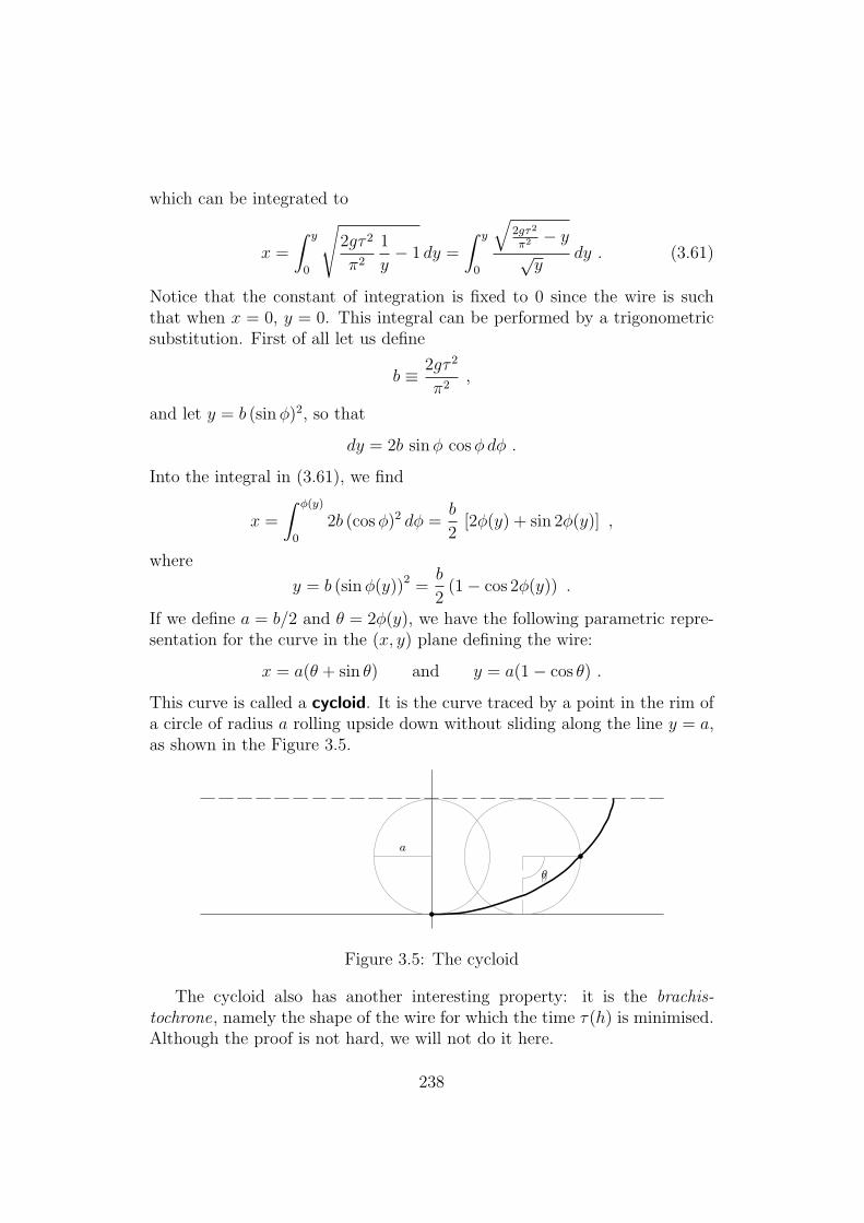
which can be integrated to

x =

∫ y

0

√2gτ 2

π2

1

y− 1 dy =

∫ y

0

√2gτ2

π2 − y√

ydy . (3.61)

Notice that the constant of integration is fixed to 0 since the wire is suchthat when x = 0, y = 0. This integral can be performed by a trigonometricsubstitution. First of all let us define

b ≡ 2gτ 2

π2,

and let y = b (sin φ)2, so that

dy = 2b sin φ cos φ dφ .

Into the integral in (3.61), we find

x =

∫ φ(y)

0

2b (cos φ)2 dφ =b

2[2φ(y) + sin 2φ(y)] ,

where

y = b (sin φ(y))2 =b

2(1− cos 2φ(y)) .

If we define a = b/2 and θ = 2φ(y), we have the following parametric repre-sentation for the curve in the (x, y) plane defining the wire:

x = a(θ + sin θ) and y = a(1− cos θ) .

This curve is called a cycloid. It is the curve traced by a point in the rim ofa circle of radius a rolling upside down without sliding along the line y = a,as shown in the Figure 3.5.

•θ

•

a •θ

Figure 3.5: The cycloid

The cycloid also has another interesting property: it is the brachis-tochrone, namely the shape of the wire for which the time τ(h) is minimised.Although the proof is not hard, we will not do it here.

238

3.3.6 The Gamma and Zeta functions

This section falls outside the main scope of these notes, but since it allows aglimpse at some of the deepest and most beautiful aspects of mathematics,I could not resist the temptation to include it.

It is possible to consider the Laplace transform of complex powers tz,with z some complex number. We see that

L tz (s) =

∫ ∞

0

tz e−st dt =1

sz+1

∫ ∞

0

uz e−u du ,

where we have changed the variable of integration from t to u = st. Let usintroduce the Euler Gamma function

Γ(z) ≡∫ ∞

0

tz−1 e−t dt , (3.62)

which converges for Re(z) > 0. Then we have that

L tz (s) =Γ(z + 1)

sz+1.

Comparing with equation (3.41), we see that Γ(n + 1) = n!, whence wecan think of the Gamma function as a way to define the factorial of a com-plex number. Although the integral representation (3.62) is only definedfor Re(z) > 0 it is possible to extend Γ(z) to a holomorphic function withonly isolated singularities in the whole complex plane: simple poles at thenonpositive integers.

To see this notice that for Re(z) > 0, we can derive a recursion relationfor Γ(z) extending the well-known n! = n (n − 1)! for positive integers n.Consider

Γ(z + 1) =

∫ ∞

0

tz e−t dt .

Integrating by parts,

Γ(z + 1) =

∫ ∞

0

z tz−1 e−t dt− tz e−t∣∣∣∞

0= z Γ(z) + lim

t→0tz e−st .

Provided that Re(z) > 0, the boundary term vanishes and we have

Γ(z + 1) = z Γ(z) . (3.63)

Turning this equation around, we have that

Γ(z) =Γ(z + 1)

z.

239

Since Γ(1) = 1, which incidentally justifies the usual claim that 0! = 1, wesee that Γ(z) has a simple pole at z = 0 with residue 1. Using this recursionrelation repeatedly, we see that Γ(z) has simple poles at all the nonpositiveintegers, with residue

Res(Γ;−k) =(−1)k

k!,

and these are all the singularities.The Gamma function is an extremely important function in mathematics,

not least of all because it is intimately related to another illustrious function:the Riemann Zeta function ζ(z), defined for Re(z) > 1 by the convergingseries

ζ(z) =∞∑

n=1

1

nz.

To see the relation notice that∫ ∞

0

tz−1 e−nt dt =1

nz

∫ ∞

0

uz−1 e−u du =Γ(z)

nz,

where we have changed variables of integration from t to u = nt. Summingboth sides of this identity over all positive integers n, we have, on the onehand ∞∑

n=1

Γ(z)

nz= Γ(z) ζ(z) ,

and on the other

∞∑n=1

∫ ∞

0

tz−1 e−nt dt =

∫ ∞

0

tz−1

∞∑n=1

e−nt dt =

∫ ∞

0

tz−1 1

et − 1dt .

where we have interchanged the summation inside the integral, and summedthe geometric series. (This can be justified, although we will not do so here.)As a result we have the following integral representation for the Zeta function

ζ(z) =1

Γ(z)

∫ ∞

0

tz−1

et − 1dt .

The only source of singularities in the integral is the zero of et − 1 at theorigin, so we can split the integral into two as follows:

ζ(z) =1

Γ(z)

[∫ 1

0

tz−1

et − 1dt +

∫ ∞

1

tz−1

et − 1dt

].

It is possible to show that Γ(z) has no zeros, whence 1/Γ(z) is entire. Simi-larly, the second integral

∫∞1

is also entire since the integrand is continuous

240

there. Hence the singularity structure of the Zeta function is contained inthe first integral. We can do a Laurent expansion of the integrand aroundt = 0:

1

et − 1=

1

t− 1

2+

t

12+ O(t3) ,

where only odd powers of t appear after the first. Therefore integratingtermwise, which we can do because Laurent series converge uniformly, wehave that ∫ 1

0

tz−1

et − 1dt =

1

z − 1− 1

2

1

z+

1

12

1

z + 1+ · · · , (3.64)

where the terms which have been omitted are all of the form ak/(z+k) where

k is a positive odd integer. This shows that the integral∫ 1

0has simple poles

at z = 1, z = 0, and z = −k with k a positive odd integer. Because theintegral is multiplied by 1/Γ(z), and the Gamma function has simple polesat the nonnegative integers we see immediately that

• ζ(z) has a simple pole at z = 1 with residue Γ(1) = 1, and is analyticeverywhere else; and

• ζ(−2n) = 0 where n is any positive integer: these are the zeros of1/Γ(z) which are not cancelled by the poles in (3.64).

The celebrated Riemann hypothesis states that all other zeros of ζ(z) occurin the line Re(z) = 1

2. Now that Fermat’s Last Theorem has been proven,

the Riemann hypothesis remains the most important open problem in math-ematics today.

The importance of settling this hypothesis stems from the intimate rela-tionship between the Zeta function and the theory of numbers. The key tothis relationship is the following infinite product expansion for ζ(z), valid forRe(z) > 1:

1

ζ(z)=

∏primes

p

(1− 1

pz

),

which follows from the unique factorisation of every positive integer into aproduct of primes. To see this notice that since, for Re(z) > 1, one has

ζ(z) = 1 +1

2z+

1

3z+

1

4z+

1

5z+ · · · ,

then it follows that

1

2zζ(z) =

1

2z+

1

4z+

1

6z+

1

8z+

1

10z+ · · · ;

241

whence (1− 1

2z

)ζ(z) = 1 +

1

3z+

1

5z+

1

7z+

1

9z+ · · · .

In other words we have in the right-hand side only those terms 1/nz wheren is odd. Similarly,

(1− 1

3z

)(1− 1

2z

)ζ(z) = 1 +

1

5z+

1

7z+

1

11z+

1

13z+ · · · ,

where now we have in the right-hand side only those terms 1/nz where n isnot divisible by 2 or by 3. Continuing in this fashion, we have that

∏primes

p

(1− 1

pz

)ζ(z) = 1 .

By the way, this shows that ζ(z) has no zeros for Re(z) > 1.The Zeta function and its generalisations also play a useful role in physics:

particularly in quantum field theory, statistical mechanics, and, of course,in string theory. In fact, together with the heat kernel, introduced in theproblems, the (generalised) Zeta function proves invaluable in computingdeterminants and traces of infinite-dimensional matrices

Areas of spheres

As a minor application of the Gamma function, let us compute the area of aunit sphere in n dimensions, for n ≥ 2.

What do we mean by a unit sphere in n dimensions? The unit spherein n dimensions is the set of points in n-dimensional euclidean space whichare a unit distance away from the origin. If we let (x1, x2, . . . , xn) be thecoordinates for euclidean space, the unit sphere is the set of points whichsatisfy the equation

n∑i=1

x2i = x2

1 + x22 + . . . x2

n = 1 .

In n = 2 dimensions, the unit “sphere” is a circle, whereas in n = 3 dimen-sions it is the usual sphere of everyday experience. For n > 3, the sphere isharder to visualise, but one can still work with it via the algebraic descriptionabove.

What do we mean by its area? We mean the n− 1-dimensional area: soif n = 2, we mean the circumference of the circle, and if n = 3 we mean

242

the usual area of everyday experience. Again it gets harder to visualise forn > 3, but one can again tackle the problem algebraically as above.

Clearly every point in n-dimensional space lies on some sphere: if it is adistance r away from the origin then, by definition, it lies on the sphere ofradius r. There are an uncountable number of spheres in euclidean space,one for every positive real number. All these spheres taken together with theorigin (a “sphere” of zero radius) make up all of euclidean space. A simplescaling argument shows that if we double the radius, we multiply the area ofthe sphere by 2n−1. More generally, the area of the sphere at radius r willbe rn−1 times the area of the unit sphere. Therefore the volume element inn-dimensions is

dnx = rn−1 dr dΩ ,

where dΩ is the area element of the unit sphere. We will now integratethe function exp(−r2) over all of the euclidean space. We can compute thisintegral in either of two ways. On the one hand,

I ≡∫· · ·

∫e−r2

dnx

=

∫· · ·

∫e−x2

1−x22−···−x2

n dx1dx2 · · · dxn

=

(∫ ∞

−∞e−x2

1 dx1

) (∫ ∞

−∞e−x2

2 dx2

)· · ·

(∫ ∞

−∞e−x2

n dxn

)

=

(∫ ∞

−∞e−x2

dx

)n

,

which is computed to give (√

π)n after using the elementary gaussian result:∫∞−∞ exp(−x2) dx =

√π. On the other hand,

I =

∫· · ·

∫e−r2

rn−1 dr dΩ =

(∫ ∞

0

e−r2

rn−1 dr

)(∫· · ·

∫dΩ

).

The integral of dΩ is simply the area A of the unit sphere, which is whatwe want to calculate. The radial integral can be calculated in terms of theGamma function after changing the variable of integration from r to t = r2:

∫ ∞

0

e−r2

rn−1 dr =

∫ ∞

0

e−t 12t(n−2)/2 dt =

Γ(n/2)

2.

Equating both ways to compute the integral, we arrive at the following for-mula for the area A(n) of the unit sphere in n dimensions:

A(n) =2 πn/2

Γ(n/2). (3.65)

243

To see that this beautiful formula is not obviously wrong, let us see thatit reproduces what we know. For n = 2, by the area of the unit sphere wemean the circumference of the unit circle, that is 2π. In n = 3, we expect thearea of the standard unit sphere and that is 4π. Let us see if our expectationsare born out. According to the formula,

A(2) =2π

Γ(1)= 2π ,

as expected. For n = 3 the formula says

A(3) =2 π3/2

Γ(3/2).

We can compute the half-integral values of the Gamma function as follows.First we have that

Γ(12) =

∫ ∞

0

t−1/2 e−t dt .

Changing variables to t = u2, we have

Γ(12) = 2

∫ ∞

0

e−u2

du =

∫ ∞

−∞e−u2

du =√

π .

Now using the recursion relation (3.63), we have that

Γ(k + 12) =

2k − 1

2

2k − 3

2· · · 1

2Γ(1

2) =

(2k − 1)!!

2k

√π .

In particular, Γ(32) =

√π

2, whence

A(3) =2π3/2

Γ(3/2)= 4π ,

as expected.

How about for n = 1? This case is a little special: in one dimension the unit sphereconsists of the points ±1. So that it is a zero-dimensional set. Is there an intrinsic notionof area for a zero-dimensional set? If we evaluate the above formula for A(n) at n = 1,we get an answer: A(1) = 2, which is counting the number of points: in other words,zero-dimensional area is simply the cardinality of the set: the number of elements. Thisis something that perhaps we would not have expected. As someone said once, someformulae are more clever than the people who come up with them.

Now that we trust the formula, we can compute a few more values tolearn something new. First let us simplify the formula by evaluating the

244

Gamma function at the appropriate values. Distinguishing between odd andeven dimensions, we find

A(n) =

2 π`

(`− 1)!, for n = 2`, and

2`+1 π`

(2`− 1)!!, for n = 2` + 1.

(3.66)

The next few values are

A(4) = 2 π2 , A(5) =8π3

3, A(6) = π3 , A(7) =

16π3

15, A(8) =

π4

3.

In case you are wondering whether this is at all useful, it actually comes in handy whennormalising electromagnetic fields in higher-dimensional field theories so that they haveintegral fluxes around charged objects (e.g., branes and black holes).

Let us end with another nice formula. How about the n-dimensionalvolume V (n) of the unit ball, i.e., the interior of the unit sphere? We cancompute this by integrating the areas of the spheres from radius 0 to radius1. The area of the sphere of radius r will be rn−1 times the area of the sphereof unit radius, so that the volume is then

V (n) =

∫ 1

0

A(n)rn−1 dr =A(n)

n.

Using the formula (3.65), we see that

V (n) =2πn/2

nΓ(n/2)=

πn/2

(n/2)Γ(n/2)=

πn/2

Γ((n + 2)/2),

where we have used the recursion formula (3.63). Because the the unit sphereis inscribed inside the cube of length 2, the ratio of the volume of the unitball to that of the cube circumscribing it is given by

%(n) =V (n)

2n=

πn/2

2n Γ(n2

+ 1).

If we were to plot this as a function of n we notice that it starts at 1 forn = 1 and then decreases quite fast, so that the ball takes up less and less ofthe volume of he cube which circumscribes it.

245