Embed Size (px)
Citation preview
APPENDIX D
CALPUFF Dispersion Model
Roberts Bank Container Expansion Project RWDI Deltaport Third Berth File: W04-127 CALPUFF Dispersion Model – Appendix D - ii - January 2005
TABLE OF CONTENTS
1.0 MODEL REQUIREMENTS............................................................................................ 1
1.1 CALPUFF MODEL DESCRIPTION ............................................................................ 2
2.0 MODEL APPLICATION ................................................................................................ 6
2.1 MODEL DOMAIN ...................................................................................................... 6
2.2 RECEPTOR LOCATIONS............................................................................................. 6
2.3 COMPOUNDS MODELLED ....................................................................................... 10
2.4 MESOPUFF CHEMISTRY ...................................................................................... 10
2.5 POINT SOURCE PARAMETERS................................................................................. 11
2.6 AREA SOURCE PARAMETERS ................................................................................. 11
2.7 LINE SOURCES (ROADS AND RAIL) ........................................................................ 12
2.8 TECHNICAL DISPERSION OPTIONS.......................................................................... 14
2.9 BUILDING EFFECTS ................................................................................................ 14
2.10 WET AND DRY DEPOSITION ................................................................................... 14
3.0 MODEL OUTPUT INTERPRETATION .................................................................... 15
3.1 SECONDARY PARTICULATE.................................................................................... 15
3.2 NOX TO NO2 CHEMISTRY....................................................................................... 15
3.3 SPECIATION OF VOCS, PAHS AND METALS .......................................................... 18
4.0 MODEL LIMITATIONS............................................................................................... 20
5.0 SUMMARY AND CONCLUSIONS ............................................................................. 21
6.0 FULL CALPUFF MODEL OPTIONS LISTING ....................................................... 22
7.0 REFERENCES................................................................................................................ 36
Roberts Bank Container Expansion Project RWDI Deltaport Third Berth File: W04-127 CALPUFF Dispersion Model – Appendix D - iii - January 2005
List of Tables
Table D-1: Major Features of the CALPUFF Model (continued on next page) ....................... 4
Table D-2: Model Domain (All Coordinates are for UTM Zone 10) ....................................... 6
Table D-3: Specific Receptors for the Human Health and Ecological Risk Assessments........ 8
Table D-4: Point Source Paramters for Dockside Emissions.................................................. 11
Table D-5: Typical Area Source Emissions Parameters ......................................................... 12
Table D-6: Speciation Data for VOC (as a Fraction of Total VOC)....................................... 19
Table D-7: Speciation Data for PAH (as a Fraction of PM10 or PM2.5) .................................. 19
Table D-8: Speciation Data for Metals (as a Fraction of PM2.5) ............................................. 20
Table D-9: Input Groups in the CALPUFF Control File. ....................................................... 22
Table D-10: CALPUFF Model Options Groups 1 and 2. ......................................................... 23
Table D-11: CALPUFF Model Options Groups 3 and 4 .......................................................... 25
Table D-12: CALPUFF Model Option Group 5 ....................................................................... 27
Table D-13: CALPUFF Model Option Groups 11.................................................................... 29
Table D-14: CALPUFF Model Option Group 12. .................................................................... 30
Table D-15: CALPUFF Model Option Groups 13, 14, and 15................................................. 33
Table D-16: CALPUFF Model Option Groups 16 and 17........................................................ 35
List of Figures
Figure D-1: Location of receptors used for the CALPUFF dispersion model. Crosses indicate
Cartesian grid points. .............................................................................................. 7
Figure D-2: Location of Specific Receptors for the Human Health and Ecological Risk
Assessments ............................................................................................................ 9
Figure D-3: Dependence of NO2/NOx Ratio on 1-hour Average NOx Concentrations from
GVRD Station T17 (Richmond South)................................................................. 16
Figure D-4: Dependence of NO2/NOx Ratio on 24-hour Average NOx Observations from
GVRD Station T17 (Richmond South)................................................................. 17
Figure D-5: Dependence of NO2/NOx Ratio on Annual Average NOx Observations from
GVRD Station T17 (Richmond South)................................................................. 18
Roberts Bank Container Expansion Project RWDI Deltaport Third Berth File: W04-127 CALPUFF Dispersion Model – Appendix D - 1 - January 2005
1.0 MODEL REQUIREMENTS
For the area of concern for the Project, the following model attributes are required:
1) Ability to handle multiple emissions sources of varying geometry, (point, area, line
volume), located in the study area;
2) Ability to handle both flat and elevated terrain features;
3) Ability to convert SO2 to sulphate (SO42-), and NOx to nitrate (NO3
-); and
4) Ability to simulate boundary layer mechanics and dispersion in coastal areas.
In accordance with recent assessments of proposed projects in BC, for example the BC Hydro
Vancouver Island Generation Project at Duke Point, and in consultation with regulatory
agencies, CALPUFF was chosen as the model with which to perform air quality modelling in the
Local Study Area (LSA). CALPUFF contains the attributes outlined above and, when applied in
full 3-D CALMET mode, it has the ability to assimilate multiple meteorological stations and to
simulate the changes in mixing height and boundary layer mechanics that result from the variable
land use and terrain in the study region.
Due to the expected changes in traffic patterns resulting from the project, the California Line
source model (CALINE) was suggested for modelling roadway emissions in the study area.
Although CALINE was developed expressly for this purpose, it is an older generation, Gaussian
plume model and has several limitations:
1) It is a plume rather than a puff model. Unlike CALPUFF it can not account for changes in
plume trajectory and boundary layer properties once emissions have travelled away from
the source. Also, CALINE does not account for causality, i.e. it does not track plumes
over several consecutive hours.
2) It is driven by point meteorology. Though point source meteorology can be extracted
from CALMET outputs, by and large CALINE cannot make full use of the CALMET
meteorological fields.
3) CALINE can only simulate dispersion of primary pollutants. It has no mechanisms for
chemical transformation, such as the formation of secondary particulate.
Roberts Bank Container Expansion Project RWDI Deltaport Third Berth File: W04-127 CALPUFF Dispersion Model – Appendix D - 2 - January 2005
4) It cannot include temporal variation of emission rates.
5) It does not accept area sources and therefore the cumulative contribution of other sources
cannot easily be derived.
Due to these limitations, CALINE was not selected for this study.
As described below, road and rail emissions were incorporated into CALPUFF in a manner that
should provide at least as much information about road emissions impacts as would have been
obtained using CALINE. In addition, CALPUFF does not share the limitations described above.
A comparison of CALINE and CALPUFF for line segments is given in Appendix E.
CALPUFF has two major options with respect to the meteorology used to drive the dispersion
calculations:
• The ISC mode assumes a uniform meteorological field over the modelling domain
during a given hour. While this is consistent with the ISC-PRIME and AERMOD models,
CALPUFF has the advantage of allowing the plume trajectory to vary from hour-to-hour
in a systematic manner.
• The CALMET mode allows for the use of a three-dimensional meteorological field over
the modelling domain during a given hour.
For this assessment, the CALPUFF model was applied using the CALMET mode option. The
methods employed in the development of the CALMET meteorological fields are described in
Appendix C.
1.1 CALPUFF MODEL DESCRIPTION
CALPUFF (Scire et al., 2000) is a multi-layer, multi-species, non-steady-state puff dispersion
model. It simulates the effects of time- and space-varying meteorological conditions on pollutant
transport, transformation and deposition. CALPUFF can use three-dimensional meteorological
fields developed by the CALMET model, or simple, single-station winds in a format consistent
with the meteorological files used to drive the ISCST3 steady-state Gaussian model. However,
Roberts Bank Container Expansion Project RWDI Deltaport Third Berth File: W04-127 CALPUFF Dispersion Model – Appendix D - 3 - January 2005
single-station ISCST3 winds do not allow CALPUFF to take advantage of its capabilities to treat
spatially varying meteorological fields.
CALPUFF contains algorithms for near-source effects such as building downwash, transitional
plume rise, partial plume penetration, sub-grid scale terrain interactions as well as longer-range
effects such as pollutant removal (wet scavenging and dry deposition), chemical transformation,
vertical wind shear, over-water transport, and coastal interaction effects. It can accommodate
arbitrarily varying point source and gridded area source emissions. Most of the algorithms
contain options to treat the physical processes at different levels of detail depending on the
model application.
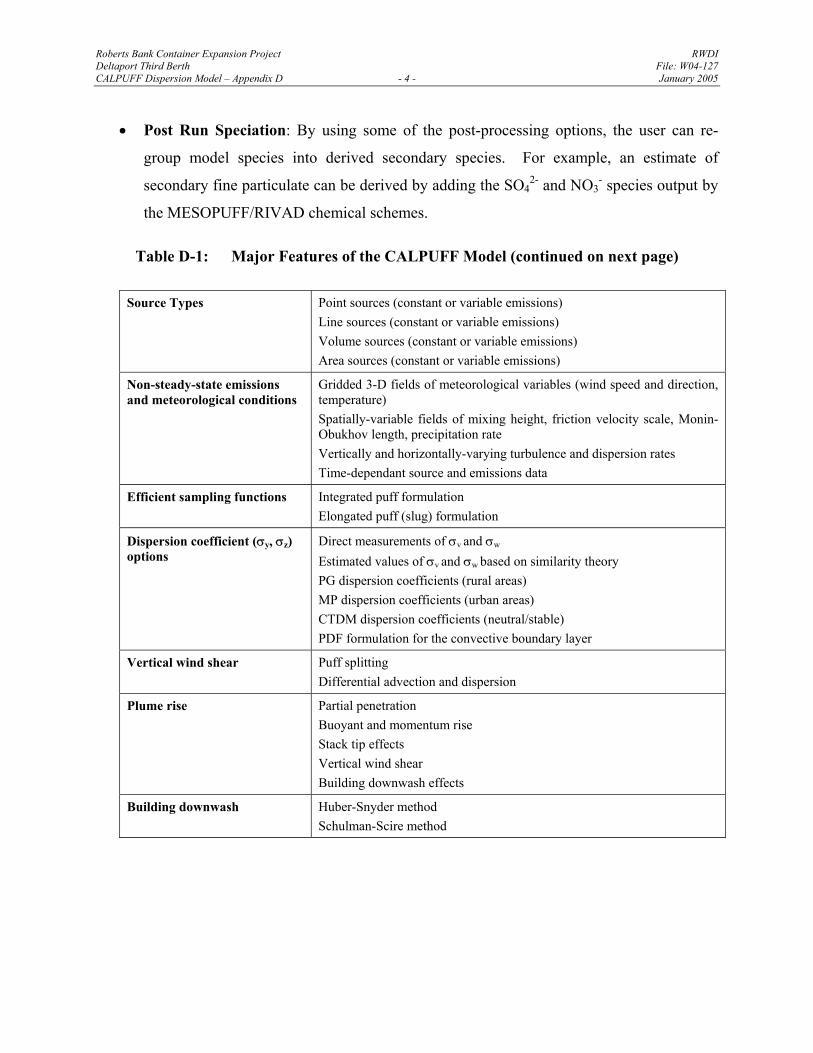
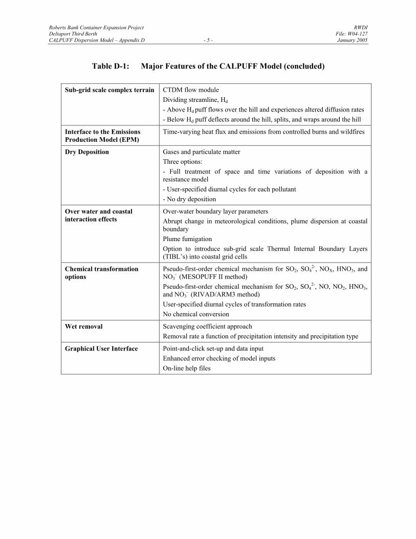
The major features and options of the CALPUFF model are summarized in Table D-1. Some of
the technical algorithms of relevance include:
• Chemical Transformation: CALPUFF includes options to parameterize chemical
transformation using the five species scheme (SO2, SO42-, NOX, HNO3, and NO3
-)
employed in the MESOPUFF II model, a modified six-species scheme (SO2, SO42-, NO,
NO2, HNO3, and NO3-) adapted from the RIVAD/ARM3 method, or a set of user-
specified, diurnally-varying transformation rates.
• Dispersion Coefficients: Several options are provided in CALPUFF for the computation
of dispersion coefficients: the use of turbulence measurements (σv and σw), similarity
theory to estimate σv and σw from modelled surface heat and momentum fluxes, Pasquill-
Gifford (PG) or McElroy-Pooler (MP) dispersion coefficients, or dispersion equations
based on the Complex Terrain Dispersion Model (CDTM). Options are provided to apply
an averaging time correction or surface roughness length adjustments to the PG
coefficients.
• Thermal Internal Boundary Layer (TIBL): For areas with transitions between water
and land, the model has the ability to simulate the growth of a thermal internal boundary
layer as the modelled air mass passes over the water/land interface.
Roberts Bank Container Expansion Project RWDI Deltaport Third Berth File: W04-127 CALPUFF Dispersion Model – Appendix D - 4 - January 2005
• Post Run Speciation: By using some of the post-processing options, the user can re-
group model species into derived secondary species. For example, an estimate of
secondary fine particulate can be derived by adding the SO42- and NO3
- species output by
the MESOPUFF/RIVAD chemical schemes.
Table D-1: Major Features of the CALPUFF Model (continued on next page)
Source Types Point sources (constant or variable emissions) Line sources (constant or variable emissions) Volume sources (constant or variable emissions) Area sources (constant or variable emissions)
Non-steady-state emissions and meteorological conditions
Gridded 3-D fields of meteorological variables (wind speed and direction, temperature) Spatially-variable fields of mixing height, friction velocity scale, Monin-Obukhov length, precipitation rate Vertically and horizontally-varying turbulence and dispersion rates Time-dependant source and emissions data
Efficient sampling functions Integrated puff formulation Elongated puff (slug) formulation
Dispersion coefficient (σy, σz) options
Direct measurements of σv and σw Estimated values of σv and σw based on similarity theory PG dispersion coefficients (rural areas) MP dispersion coefficients (urban areas) CTDM dispersion coefficients (neutral/stable) PDF formulation for the convective boundary layer
Vertical wind shear Puff splitting Differential advection and dispersion
Plume rise Partial penetration Buoyant and momentum rise Stack tip effects Vertical wind shear Building downwash effects
Building downwash Huber-Snyder method Schulman-Scire method
Roberts Bank Container Expansion Project RWDI Deltaport Third Berth File: W04-127 CALPUFF Dispersion Model – Appendix D - 5 - January 2005
Table D-1: Major Features of the CALPUFF Model (concluded)
Sub-grid scale complex terrain CTDM flow module Dividing streamline, Hd
- Above Hd puff flows over the hill and experiences altered diffusion rates - Below Hd puff deflects around the hill, splits, and wraps around the hill
Interface to the Emissions Production Model (EPM)
Time-varying heat flux and emissions from controlled burns and wildfires
Dry Deposition Gases and particulate matter Three options: - Full treatment of space and time variations of deposition with a resistance model - User-specified diurnal cycles for each pollutant - No dry deposition
Over water and coastal interaction effects
Over-water boundary layer parameters Abrupt change in meteorological conditions, plume dispersion at coastal boundary Plume fumigation Option to introduce sub-grid scale Thermal Internal Boundary Layers (TIBL’s) into coastal grid cells
Chemical transformation options
Pseudo-first-order chemical mechanism for SO2, SO42-, NOX, HNO3, and
NO3- (MESOPUFF II method)
Pseudo-first-order chemical mechanism for SO2, SO42-, NO, NO2, HNO3,
and NO3- (RIVAD/ARM3 method)
User-specified diurnal cycles of transformation rates No chemical conversion
Wet removal Scavenging coefficient approach Removal rate a function of precipitation intensity and precipitation type
Graphical User Interface Point-and-click set-up and data input Enhanced error checking of model inputs On-line help files
Roberts Bank Container Expansion Project RWDI Deltaport Third Berth File: W04-127 CALPUFF Dispersion Model – Appendix D - 6 - January 2005
2.0 MODEL APPLICATION
2.1 MODEL DOMAIN
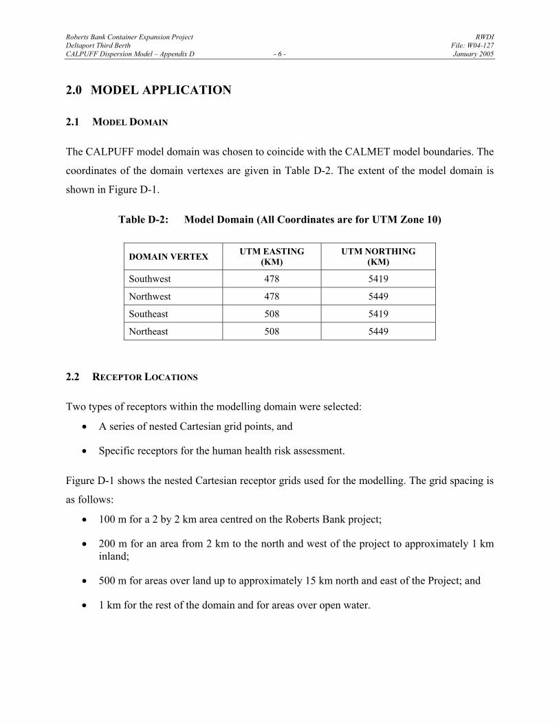
The CALPUFF model domain was chosen to coincide with the CALMET model boundaries. The
coordinates of the domain vertexes are given in Table D-2. The extent of the model domain is
shown in Figure D-1.
Table D-2: Model Domain (All Coordinates are for UTM Zone 10)
DOMAIN VERTEX UTM EASTING (KM)
UTM NORTHING (KM)
Southwest 478 5419
Northwest 478 5449
Southeast 508 5419
Northeast 508 5449
2.2 RECEPTOR LOCATIONS
Two types of receptors within the modelling domain were selected:
• A series of nested Cartesian grid points, and
• Specific receptors for the human health risk assessment.
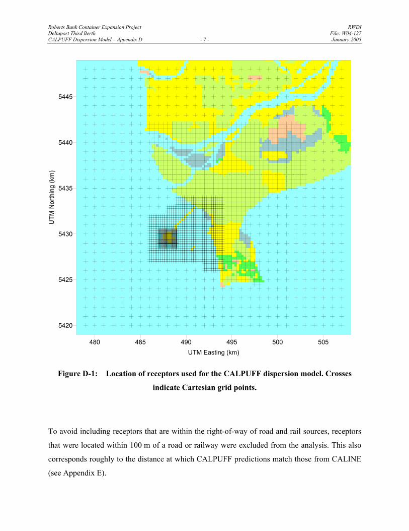
Figure D-1 shows the nested Cartesian receptor grids used for the modelling. The grid spacing is
as follows:
• 100 m for a 2 by 2 km area centred on the Roberts Bank project;
• 200 m for an area from 2 km to the north and west of the project to approximately 1 km inland;
• 500 m for areas over land up to approximately 15 km north and east of the Project; and
• 1 km for the rest of the domain and for areas over open water.
Roberts Bank Container Expansion Project RWDI Deltaport Third Berth File: W04-127 CALPUFF Dispersion Model – Appendix D - 7 - January 2005
480 485 490 495 500 505UTM Easting (km)
5420
5425
5430
5435
5440
5445
UTM
Nor
thin
g (k
m)
Figure D-1: Location of receptors used for the CALPUFF dispersion model. Crosses
indicate Cartesian grid points.
To avoid including receptors that are within the right-of-way of road and rail sources, receptors
that were located within 100 m of a road or railway were excluded from the analysis. This also
corresponds roughly to the distance at which CALPUFF predictions match those from CALINE
(see Appendix E).
Roberts Bank Container Expansion Project RWDI Deltaport Third Berth File: W04-127 CALPUFF Dispersion Model – Appendix D - 8 - January 2005
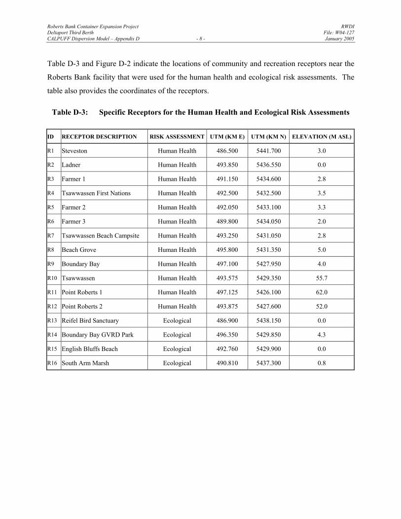
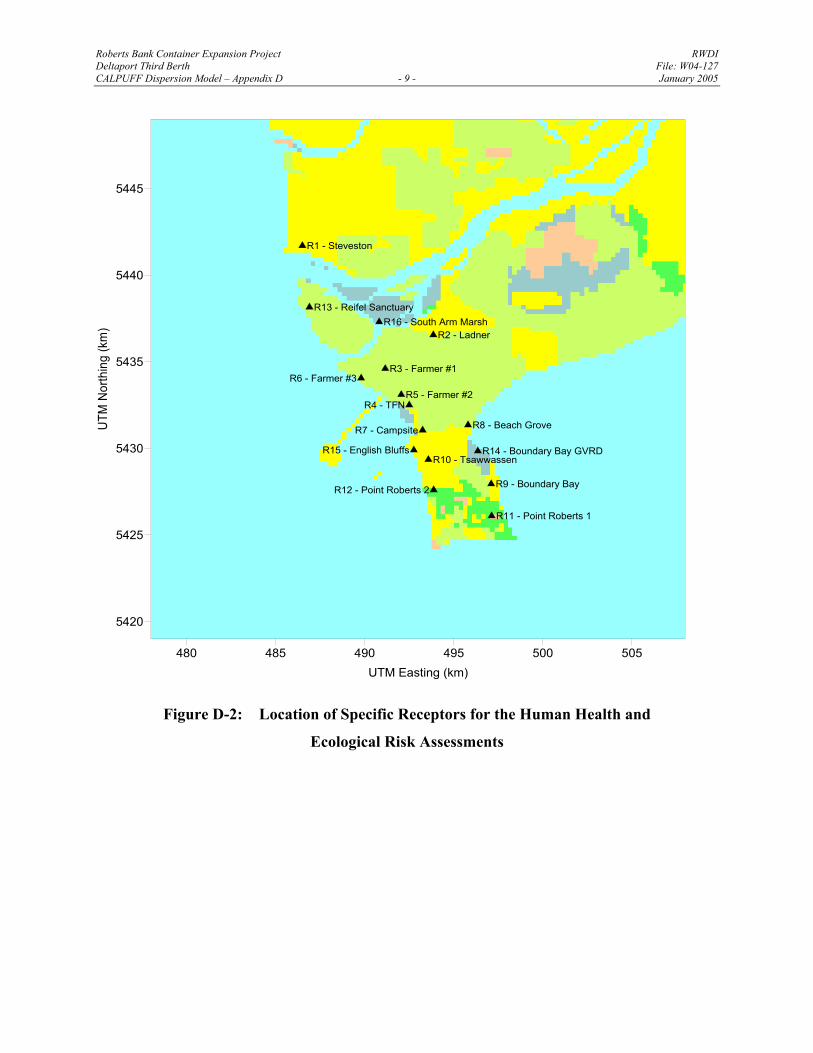
Table D-3 and Figure D-2 indicate the locations of community and recreation receptors near the
Roberts Bank facility that were used for the human health and ecological risk assessments. The
table also provides the coordinates of the receptors.
Table D-3: Specific Receptors for the Human Health and Ecological Risk Assessments
ID RECEPTOR DESCRIPTION RISK ASSESSMENT UTM (KM E) UTM (KM N) ELEVATION (M ASL)
R1 Steveston Human Health 486.500 5441.700 3.0
R2 Ladner Human Health 493.850 5436.550 0.0
R3 Farmer 1 Human Health 491.150 5434.600 2.8
R4 Tsawwassen First Nations Human Health 492.500 5432.500 3.5
R5 Farmer 2 Human Health 492.050 5433.100 3.3
R6 Farmer 3 Human Health 489.800 5434.050 2.0
R7 Tsawwassen Beach Campsite Human Health 493.250 5431.050 2.8
R8 Beach Grove Human Health 495.800 5431.350 5.0
R9 Boundary Bay Human Health 497.100 5427.950 4.0
R10 Tsawwassen Human Health 493.575 5429.350 55.7
R11 Point Roberts 1 Human Health 497.125 5426.100 62.0
R12 Point Roberts 2 Human Health 493.875 5427.600 52.0
R13 Reifel Bird Sanctuary Ecological 486.900 5438.150 0.0
R14 Boundary Bay GVRD Park Ecological 496.350 5429.850 4.3
R15 English Bluffs Beach Ecological 492.760 5429.900 0.0
R16 South Arm Marsh Ecological 490.810 5437.300 0.8
Roberts Bank Container Expansion Project RWDI Deltaport Third Berth File: W04-127 CALPUFF Dispersion Model – Appendix D - 9 - January 2005
480 485 490 495 500 505UTM Easting (km)
5420
5425
5430
5435
5440
5445
UTM
Nor
thin
g (k
m)
R4 - TFN
R6 - Farmer #3
R7 - Campsite
R12 - Point Roberts 2
R15 - English Bluffs
R1 - Steveston
R2 - Ladner
R3 - Farmer #1
R5 - Farmer #2
R8 - Beach Grove
R9 - Boundary Bay
R10 - Tsawwassen
R11 - Point Roberts 1
R13 - Reifel Sanctuary
R14 - Boundary Bay GVRD
R16 - South Arm Marsh
Figure D-2: Location of Specific Receptors for the Human Health and
Ecological Risk Assessments
Roberts Bank Container Expansion Project RWDI Deltaport Third Berth File: W04-127 CALPUFF Dispersion Model – Appendix D - 10 - January 2005
2.3 COMPOUNDS MODELLED
There were 11 compounds included in the model runs. The following 10 compounds were
modelled for both the gridded receptors and the specific receptors for the human health and
ecological risk assessments:
SO2, SO42-, NOx , NO-
3, HNO3, PM2.5, PM10, TSP, VOCs and CO.
For the receptor grid runs, non-reactive inert NOx (i.e., emitted at the same rate as NOx but not
included in the chemical transformations) was included as an 11th compound. For the human
health assessment, Diesel PM (PM2.5 resulting from combustion of diesel fuels only) was
included as the 11th compound.
For all sources, the emissions rates of SO42-, NO-
3 and HNO3 were set to zero. Predicted
concentrations of these compound are purely the result of secondary chemical reactions.
2.4 MESOPUFF CHEMISTRY
The MESOPUFF II chemistry option was used to calculate concentrations of secondary nitrate
and sulphate. This option is the US EPA regulatory default. Hourly observed ozone
concentrations from GVRD station T17 were used to supply the background ozone concentration
required by the MESOPUFF II scheme. The model also requires background concentrations of
ammonium. A wide range of ammonium concentrations have been measured in the Lower
Fraser Valley. As part of a field campaign in July and August 1993, ammonium concentrations
ranging from 0 to 4 µg/m3 were observed at three sites: Chilliwack, Clearbrook and Pitt
Meadows (Barthelmie and Pryor, 1998). Ammonium concentrations were also measured at two
sites in the eastern past of the Lower Fraser Valley, an area known for its high ammonia
emissions from agricultural sources, from February 1996 to March 1997 (Belzer et al., 1997).
Ammonia concentrations ranged from about 8 to 30 µg/m3 at the Abbotsford site, and from about
2 to 10 µg/m3 at the Agassiz site. The CALPUFF default background ammonium concentration
of 10 ppb (7 µg/m3) is bracketed by these historical observations and was used for this project.
Roberts Bank Container Expansion Project RWDI Deltaport Third Berth File: W04-127 CALPUFF Dispersion Model – Appendix D - 11 - January 2005
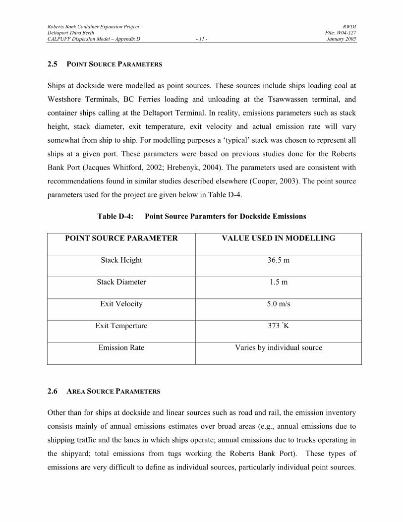
2.5 POINT SOURCE PARAMETERS
Ships at dockside were modelled as point sources. These sources include ships loading coal at
Westshore Terminals, BC Ferries loading and unloading at the Tsawwassen terminal, and
container ships calling at the Deltaport Terminal. In reality, emissions parameters such as stack
height, stack diameter, exit temperature, exit velocity and actual emission rate will vary
somewhat from ship to ship. For modelling purposes a ‘typical’ stack was chosen to represent all
ships at a given port. These parameters were based on previous studies done for the Roberts
Bank Port (Jacques Whitford, 2002; Hrebenyk, 2004). The parameters used are consistent with
recommendations found in similar studies described elsewhere (Cooper, 2003). The point source
parameters used for the project are given below in Table D-4.
Table D-4: Point Source Paramters for Dockside Emissions
POINT SOURCE PARAMETER VALUE USED IN MODELLING
Stack Height 36.5 m
Stack Diameter 1.5 m
Exit Velocity 5.0 m/s
Exit Temperture 373 ◦K
Emission Rate Varies by individual source
2.6 AREA SOURCE PARAMETERS
Other than for ships at dockside and linear sources such as road and rail, the emission inventory
consists mainly of annual emissions estimates over broad areas (e.g., annual emissions due to
shipping traffic and the lanes in which ships operate; annual emissions due to trucks operating in
the shipyard; total emissions from tugs working the Roberts Bank Port). These types of
emissions are very difficult to define as individual sources, particularly individual point sources.
Roberts Bank Container Expansion Project RWDI Deltaport Third Berth File: W04-127 CALPUFF Dispersion Model – Appendix D - 12 - January 2005
Even where the emissions are from a point source, such as the stack of a ship or ferry at sea, the
location of the source varies too quickly to be defined on an hour-by-hour basis. All such
emissions were treated as area sources.
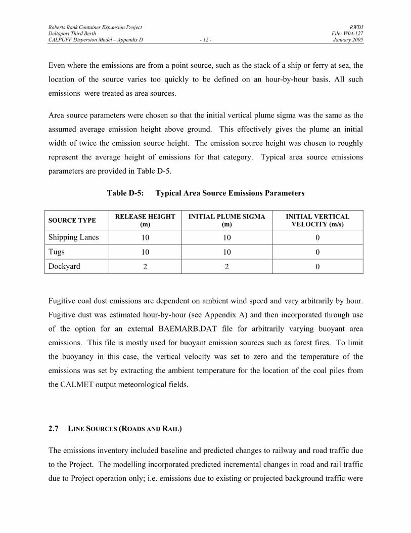
Area source parameters were chosen so that the initial vertical plume sigma was the same as the
assumed average emission height above ground. This effectively gives the plume an initial
width of twice the emission source height. The emission source height was chosen to roughly
represent the average height of emissions for that category. Typical area source emissions
parameters are provided in Table D-5.
Table D-5: Typical Area Source Emissions Parameters
SOURCE TYPE RELEASE HEIGHT (m)
INITIAL PLUME SIGMA (m)
INITIAL VERTICAL VELOCITY (m/s)
Shipping Lanes 10 10 0
Tugs 10 10 0
Dockyard 2 2 0
Fugitive coal dust emissions are dependent on ambient wind speed and vary arbitrarily by hour.
Fugitive dust was estimated hour-by-hour (see Appendix A) and then incorporated through use
of the option for an external BAEMARB.DAT file for arbitrarily varying buoyant area
emissions. This file is mostly used for buoyant emission sources such as forest fires. To limit
the buoyancy in this case, the vertical velocity was set to zero and the temperature of the
emissions was set by extracting the ambient temperature for the location of the coal piles from
the CALMET output meteorological fields.
2.7 LINE SOURCES (ROADS AND RAIL)
The emissions inventory included baseline and predicted changes to railway and road traffic due
to the Project. The modelling incorporated predicted incremental changes in road and rail traffic
due to Project operation only; i.e. emissions due to existing or projected background traffic were
Roberts Bank Container Expansion Project RWDI Deltaport Third Berth File: W04-127 CALPUFF Dispersion Model – Appendix D - 13 - January 2005
not included in the modelling as they were accounted for by adding the 98th percentile ambient
observed values. Rail and roadway emissions were implemented in CALPUFF as line sources.
CALPUFF uses the Buoyant Line Source Algorithm (Scire, 2000). The model developers
intended for this algorithm to be used for elongated buoyant line sources (such as building roof
vents) and recommend using area or volume sources to model road sources.
However, CALPUFF uses the ISC2 area source algorithm (Scire, 2000). Model guidance for use
of this algorithm dictates that the ratio of length to width for rectangular area sources should not
exceed 10:1. There are over 80 km of road and railway included in each scenario. Even
assuming a rather wide average source width of 50 m would result in upwards of 160 area
sources in addition to those from non-road and rail emissions. Area sources are very
computationally expensive and this many sources would make model run times untenable.
Although the line source algorithm used in CALPUFF was not designed for modelling road
sources, by selecting parameters to limit the buoyancy of the line source plume, the algorithm
can be made to approximate results obtained from using line sources in ISC or AERMOD
(Radonjic et al, 2003).
Use of line sources reduces the total number of separate road and rail segments to a maximum of
35. In addition, each individual line source is not as computationally intensive as a
corresponding area source. Although each line source still releases a very large number of puffs
at each hour and the CALPUFF simulation requires very significant computer resources, the
resulting run time is about an order of magnitude less than would be required for modelling using
area sources.
A comparison of resulting predicted concentrations from road emissions using CALPPUFF line
sources versus the same sources in CALINE is provided in Appendix E. In general, CALPUFF
was found to predict higher concentrations compared to CALINE for locations within
approximately 200 m of the source centerline. For locations at 500 m from the source centerline
and beyond, CALPUFF and CALINE provided similar results.
Roberts Bank Container Expansion Project RWDI Deltaport Third Berth File: W04-127 CALPUFF Dispersion Model – Appendix D - 14 - January 2005
Line source parameters for input to CALPUFF were adjusted to mimic a non-buoyant plume.
Also line sources were entered so as to avoid invoking calculations in the BLP algorithm for
parameters such as building height and distance between line sources. This was done by
defining each individual line segment as its own source group containing just the one line
segment, and incorporating all line sources through use of the external LNEMARB.DAT
emissions file. This required recompiling CALPUFF to allow for more line source groups than
the default configuration. This change in array size only affects the number of sources that may
be included and does not affect any of the actual plume dispersion calculations.
2.8 TECHNICAL DISPERSION OPTIONS
In the absence of regulatory guidance to the contrary, all technical options relating to the
CALPUFF dispersion calculation were set to the model defaults. These include parameters and
options such as the calculation of plume dispersion coefficients, the plume path coefficients used
for terrain adjustments, exponents for the wind speed profile, and wind speed categories. These
options are listed in their entirety in Tables D-8 through D-15.
2.9 BUILDING EFFECTS
All sources in the models were entered as area or line sources. No building downwash
information was required.
2.10 WET AND DRY DEPOSITION
Wet and dry deposition was not modelled for this assessment. As a result, with no removal
processes, predicted concentrations, most notably of particulate, are conservative in nature.
Roberts Bank Container Expansion Project RWDI Deltaport Third Berth File: W04-127 CALPUFF Dispersion Model – Appendix D - 15 - January 2005
3.0 MODEL OUTPUT INTERPRETATION
3.1 SECONDARY PARTICULATE
In addition to the compounds explicitly included in the model, secondary particulate species
were derived from the outputs of secondary SO42- and NO3
-. To calculate the mass of secondary
particulate matter, it was conservatively assumed that the sulphate and nitrate ions would
combine with ambient ammonium ions (NH4+) to form (NH4)2SO4 and (NH4)NO3. It was further
assumed that the resulting (NH4)2SO4 and (NH4)NO3 particles would be less than 2.5 microns in
diameter and thus would add to the predicted primary PM2.5 concentrations.
The calculated secondary PM2.5 concentrations were then added to each of the primary PM2.5,
PM10 and TSP concentrations to estimate totals of primary plus secondary particulate (denoted
PM2.5sec, PM10sec and TSPsec, respectively) for each of the three particulate size classes.
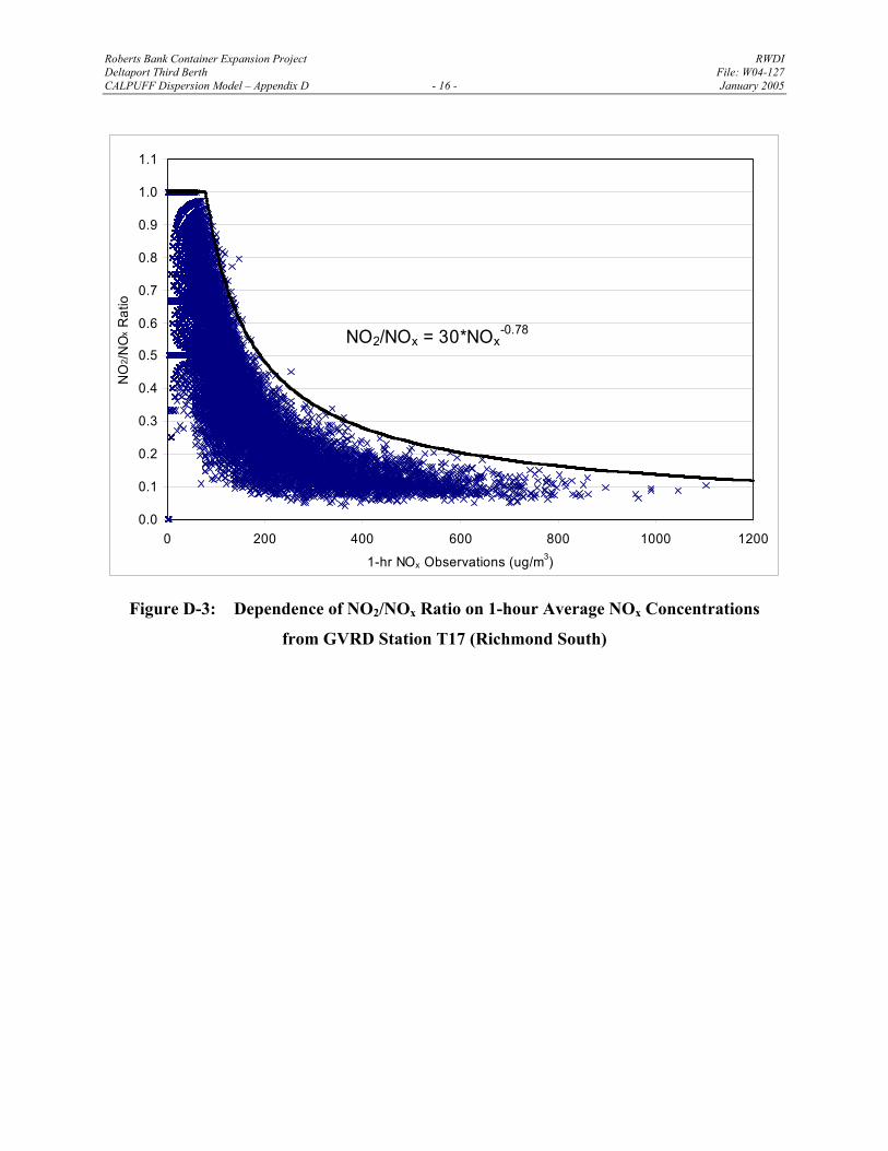
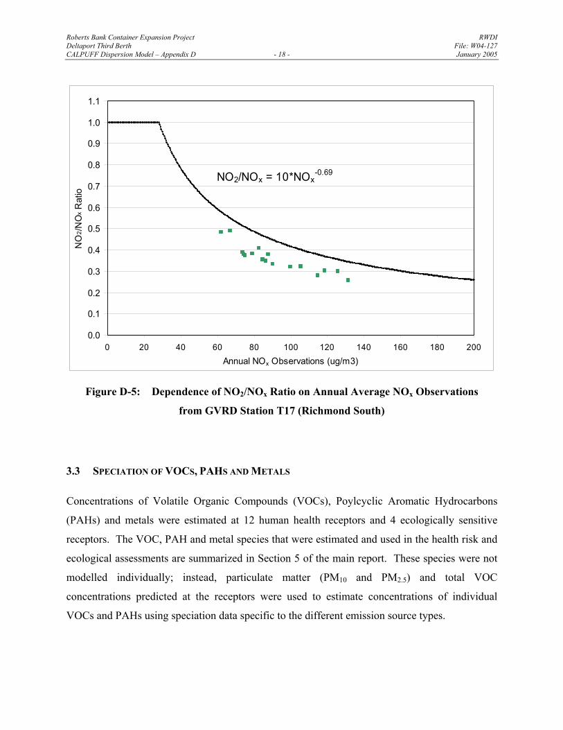
3.2 NOX TO NO2 CHEMISTRY
For this assessment, NO2 concentrations were estimated from the predicted total NOx
concentrations using the ambient ratio method. The ambient ratio method relies on obtaining an
estimate of the NO2/NOx ratio based on representative ambient observations. Ambient air
quality data from GVRD station T17 (Richmond South) were used to calculate the NO2/NOx
ratios. The resulting ratios were validated against ambient observations from GVRD stations T2
(Kitsilano) and T31 (Vancouver Airport).
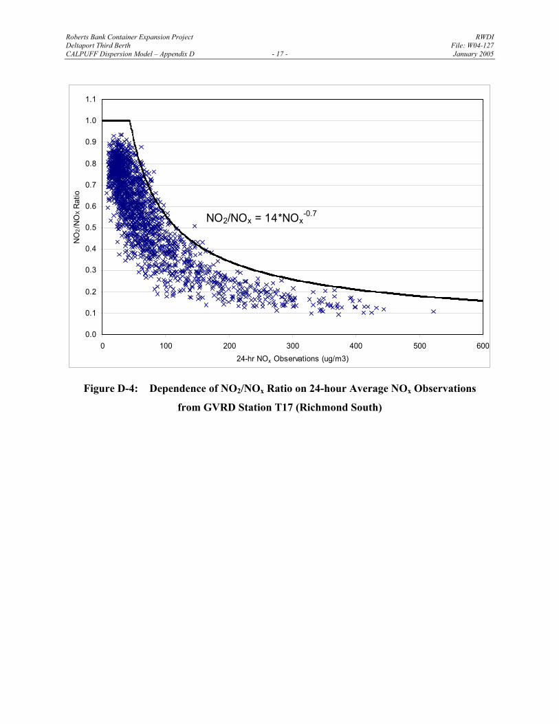
For each averaging period (1-hour, 24-hour and annual), curves were fit to the upper-envelope of
observed NO2/NOx versus NOx. The resulting relationships are depicted in Figure D-3, D-4 and
D-5 for the one-hour, 24-hour and annual average concentrations. The curve on each plot is an
exponential of the form baxy = , where a and b are empirically determined parameters. The
equation given for each averaging period is used to determine the ratio of NO2/NOx for a
predicted NOx concentration, subject to the conditions that: 1) The calculated NO2/NOx ratio
may never exceed unity, and 2) the calculated NO2/NOx ratio may never be less than 0.10.
Roberts Bank Container Expansion Project RWDI Deltaport Third Berth File: W04-127 CALPUFF Dispersion Model – Appendix D - 16 - January 2005
0.0
0.1
0.2
0.3
0.4
0.5
0.6
0.7
0.8
0.9
1.0
1.1
0 200 400 600 800 1000 1200
1-hr NOx Observations (ug/m3)
NO
2 /NO
x Rat
io
NO2/NOx = 30*NOx-0.78
Figure D-3: Dependence of NO2/NOx Ratio on 1-hour Average NOx Concentrations
from GVRD Station T17 (Richmond South)
Roberts Bank Container Expansion Project RWDI Deltaport Third Berth File: W04-127 CALPUFF Dispersion Model – Appendix D - 17 - January 2005
0.0
0.1
0.2
0.3
0.4
0.5
0.6
0.7
0.8
0.9
1.0
1.1
0 100 200 300 400 500 60024-hr NOx Observations (ug/m3)
NO
2/N
OX
Rat
io
NO2/NOx = 14*NOx-0.7
Figure D-4: Dependence of NO2/NOx Ratio on 24-hour Average NOx Observations
from GVRD Station T17 (Richmond South)
Roberts Bank Container Expansion Project RWDI Deltaport Third Berth File: W04-127 CALPUFF Dispersion Model – Appendix D - 18 - January 2005
0.0
0.1
0.2
0.3
0.4
0.5
0.6
0.7
0.8
0.9
1.0
1.1
0 20 40 60 80 100 120 140 160 180 200Annual NOx Observations (ug/m3)
NO
2 /NO
x Rat
io
NO2/NOx = 10*NOx-0.69
Figure D-5: Dependence of NO2/NOx Ratio on Annual Average NOx Observations
from GVRD Station T17 (Richmond South)
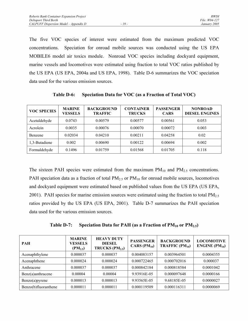
3.3 SPECIATION OF VOCS, PAHS AND METALS
Concentrations of Volatile Organic Compounds (VOCs), Poylcyclic Aromatic Hydrocarbons
(PAHs) and metals were estimated at 12 human health receptors and 4 ecologically sensitive
receptors. The VOC, PAH and metal species that were estimated and used in the health risk and
ecological assessments are summarized in Section 5 of the main report. These species were not
modelled individually; instead, particulate matter (PM10 and PM2.5) and total VOC
concentrations predicted at the receptors were used to estimate concentrations of individual
VOCs and PAHs using speciation data specific to the different emission source types.
Roberts Bank Container Expansion Project RWDI Deltaport Third Berth File: W04-127 CALPUFF Dispersion Model – Appendix D - 19 - January 2005
The five VOC species of interest were estimated from the maximum predicted VOC
concentrations. Speciation for onroad mobile sources was conducted using the US EPA
MOBILE6 model air toxics module. Nonroad VOC species including dockyard equipment,
marine vessels and locomotives were estimated using fraction to total VOC ratios published by
the US EPA (US EPA, 2004a and US EPA, 1998). Table D-6 summarizes the VOC speciation
data used for the various emission sources.
Table D-6: Speciation Data for VOC (as a Fraction of Total VOC)
VOC SPECIES MARINE VESSELS
BACKGROUND TRAFFIC
CONTAINER TRUCKS
PASSENGER CARS
NONROAD DIESEL ENGINES
Acetaldehyde 0.0743 0.00579 0.00577 0.00561 0.053
Acrolein 0.0035 0.00076 0.00070 0.00072 0.003
Benzene 0.02034 0.04210 0.00211 0.04258 0.02
1,3-Butadiene 0.002 0.00690 0.00122 0.00694 0.002
Formaldehyde 0.1496 0.01759 0.01568 0.01705 0.118
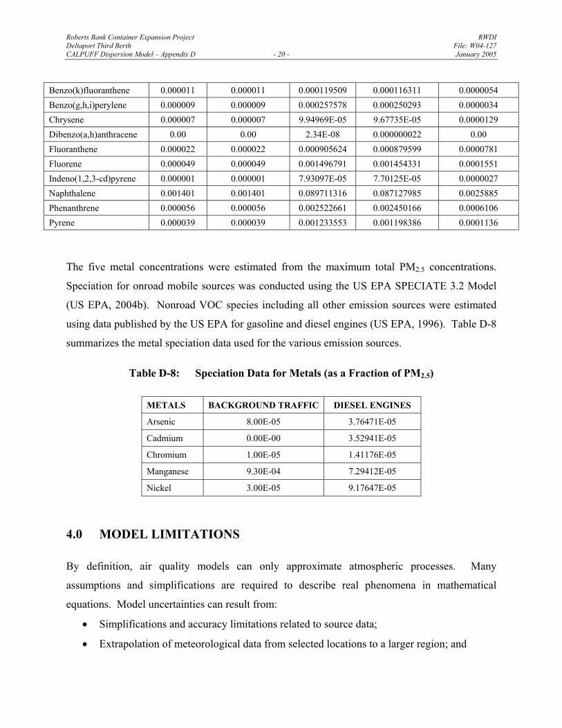
The sixteen PAH species were estimated from the maximum PM10 and PM2.5 concentrations.
PAH speciation data as a fraction of total PM2.5 or PM10 for onroad mobile sources, locomotives
and dockyard equipment were estimated based on published values from the US EPA (US EPA,
2001). PAH species for marine emission sources were estimated using the fraction to total PM2.5
ratios provided by the US EPA (US EPA, 2001). Table D-7 summarizes the PAH speciation
data used for the various emission sources.
Table D-7: Speciation Data for PAH (as a Fraction of PM10 or PM2.5)
PAH MARINE VESSELS
(PM2.5)
HEAVY DUTY DIESEL
TRUCKS (PM2.5)
PASSENGER CARS (PM10)
BACKGROUND TRAFFIC (PM10)
LOCOMOTIVE ENGINE (PM10)
Acenaphthylene 0.000037 0.000037 0.004083157 0.003964501 0.0004355 Acenaphthene 0.000024 0.000024 0.000722465 0.000702016 0.000037 Anthracene 0.000037 0.000037 0.000842184 0.000818584 0.0001042 Benz(a)anthracene 0.00004 0.00004 9.93916E-05 0.000097648 0.0000166 Benzo(a)pyrene 0.000013 0.000013 9.93565E-05 9.68185E-05 0.0000027 Benzo(b)fluoranthene 0.000011 0.000011 0.000119509 0.000116311 0.0000069
Roberts Bank Container Expansion Project RWDI Deltaport Third Berth File: W04-127 CALPUFF Dispersion Model – Appendix D - 20 - January 2005
Benzo(k)fluoranthene 0.000011 0.000011 0.000119509 0.000116311 0.0000054 Benzo(g,h,i)perylene 0.000009 0.000009 0.000257578 0.000250293 0.0000034 Chrysene 0.000007 0.000007 9.94969E-05 9.67735E-05 0.0000129 Dibenzo(a,h)anthracene 0.00 0.00 2.34E-08 0.000000022 0.00 Fluoranthene 0.000022 0.000022 0.000905624 0.000879599 0.0000781 Fluorene 0.000049 0.000049 0.001496791 0.001454331 0.0001551 Indeno(1,2,3-cd)pyrene 0.000001 0.000001 7.93097E-05 7.70125E-05 0.0000027 Naphthalene 0.001401 0.001401 0.089711316 0.087127985 0.0025885 Phenanthrene 0.000056 0.000056 0.002522661 0.002450166 0.0006106 Pyrene 0.000039 0.000039 0.001233553 0.001198386 0.0001136
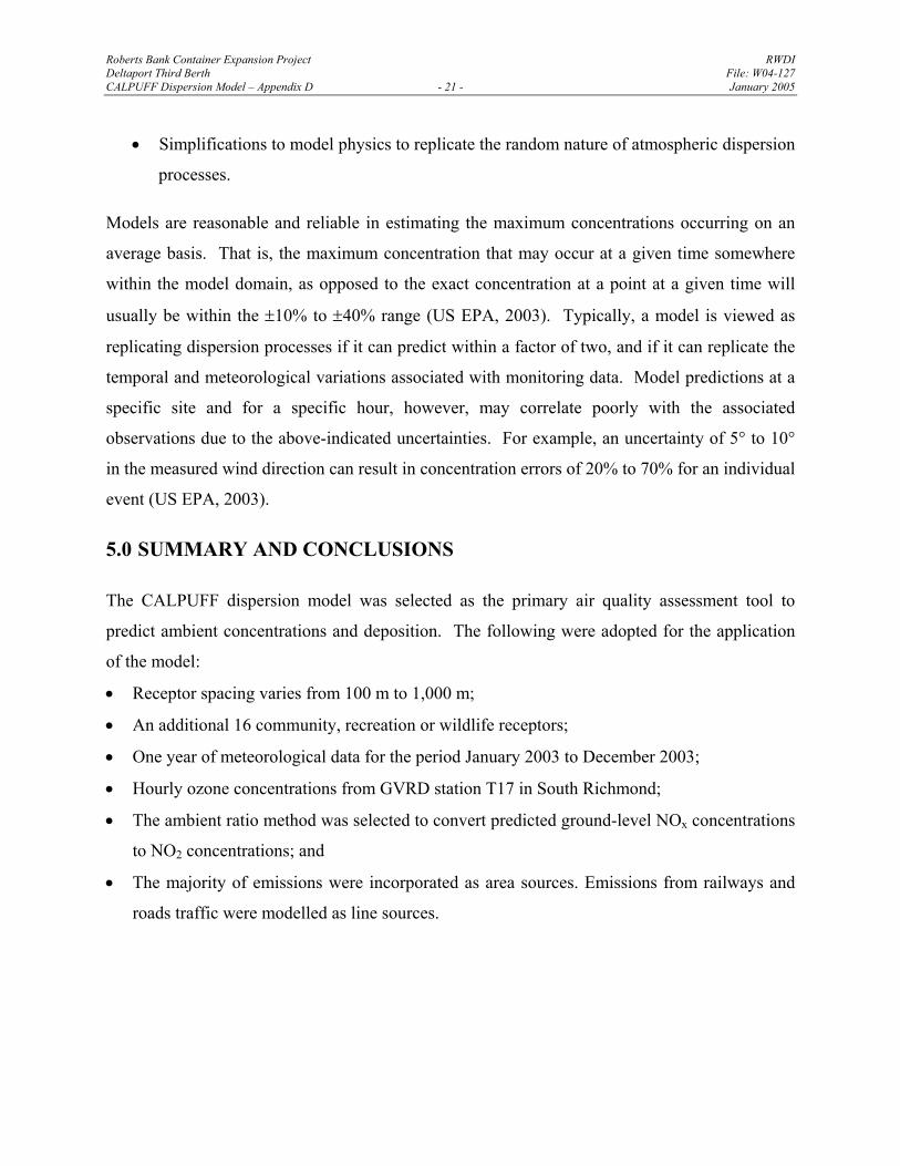
The five metal concentrations were estimated from the maximum total PM2.5 concentrations.
Speciation for onroad mobile sources was conducted using the US EPA SPECIATE 3.2 Model
(US EPA, 2004b). Nonroad VOC species including all other emission sources were estimated
using data published by the US EPA for gasoline and diesel engines (US EPA, 1996). Table D-8
summarizes the metal speciation data used for the various emission sources.
Table D-8: Speciation Data for Metals (as a Fraction of PM2.5)
METALS BACKGROUND TRAFFIC DIESEL ENGINES
Arsenic 8.00E-05 3.76471E-05
Cadmium 0.00E-00 3.52941E-05
Chromium 1.00E-05 1.41176E-05
Manganese 9.30E-04 7.29412E-05
Nickel 3.00E-05 9.17647E-05
4.0 MODEL LIMITATIONS
By definition, air quality models can only approximate atmospheric processes. Many
assumptions and simplifications are required to describe real phenomena in mathematical
equations. Model uncertainties can result from:
• Simplifications and accuracy limitations related to source data;
• Extrapolation of meteorological data from selected locations to a larger region; and
Roberts Bank Container Expansion Project RWDI Deltaport Third Berth File: W04-127 CALPUFF Dispersion Model – Appendix D - 21 - January 2005
• Simplifications to model physics to replicate the random nature of atmospheric dispersion
processes.
Models are reasonable and reliable in estimating the maximum concentrations occurring on an
average basis. That is, the maximum concentration that may occur at a given time somewhere
within the model domain, as opposed to the exact concentration at a point at a given time will
usually be within the ±10% to ±40% range (US EPA, 2003). Typically, a model is viewed as
replicating dispersion processes if it can predict within a factor of two, and if it can replicate the
temporal and meteorological variations associated with monitoring data. Model predictions at a
specific site and for a specific hour, however, may correlate poorly with the associated
observations due to the above-indicated uncertainties. For example, an uncertainty of 5° to 10°
in the measured wind direction can result in concentration errors of 20% to 70% for an individual
event (US EPA, 2003).
5.0 SUMMARY AND CONCLUSIONS
The CALPUFF dispersion model was selected as the primary air quality assessment tool to
predict ambient concentrations and deposition. The following were adopted for the application
of the model:
• Receptor spacing varies from 100 m to 1,000 m;
• An additional 16 community, recreation or wildlife receptors;
• One year of meteorological data for the period January 2003 to December 2003;
• Hourly ozone concentrations from GVRD station T17 in South Richmond;
• The ambient ratio method was selected to convert predicted ground-level NOx concentrations
to NO2 concentrations; and
• The majority of emissions were incorporated as area sources. Emissions from railways and
roads traffic were modelled as line sources.
Roberts Bank Container Expansion Project RWDI Deltaport Third Berth File: W04-127 CALPUFF Dispersion Model – Appendix D - 22 - January 2005
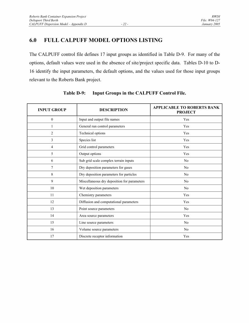
6.0 FULL CALPUFF MODEL OPTIONS LISTING
The CALPUFF control file defines 17 input groups as identified in Table D-9. For many of the
options, default values were used in the absence of site/project specific data. Tables D-10 to D-
16 identify the input parameters, the default options, and the values used for those input groups
relevant to the Roberts Bank project.
Table D-9: Input Groups in the CALPUFF Control File.
INPUT GROUP DESCRIPTION APPLICABLE TO ROBERTS BANK PROJECT
0 Input and output file names Yes
1 General run control parameters Yes
2 Technical options Yes
3 Species list Yes
4 Grid control parameters Yes
5 Output options Yes
6 Sub grid scale complex terrain inputs No
7 Dry deposition parameters for gases No
8 Dry deposition parameters for particles No
9 Miscellaneous dry deposition for parameters No
10 Wet deposition parameters No
11 Chemistry parameters Yes
12 Diffusion and computational parameters Yes
13 Point source parameters No
14 Area source parameters Yes
15 Line source parameters No
16 Volume source parameters No
17 Discrete receptor information Yes
Roberts Bank Container Expansion Project RWDI Deltaport Third Berth File: W04-127 CALPUFF Dispersion Model – Appendix D - 23 - January 2005
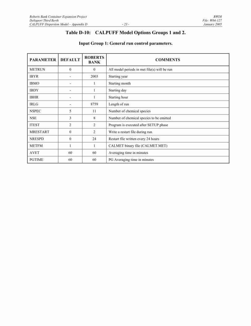
Table D-10: CALPUFF Model Options Groups 1 and 2.
Input Group 1: General run control parameters.
PARAMETER DEFAULT ROBERTS BANK COMMENTS
METRUN 0 0 All model periods in met file(s) will be run
IBYR - 2003 Starting year
IBMO - 1 Starting month
IBDY - 1 Starting day
IBHR - 1 Starting hour
IRLG - 8759 Length of run
NSPEC 5 11 Number of chemical species
NSE 3 8 Number of chemical species to be emitted
ITEST 2 2 Program is executed after SETUP phase
MRESTART 0 2 Write a restart file during run
NRESPD 0 24 Restart file written every 24 hours
METFM 1 1 CALMET binary file (CALMET.MET)
AVET 60 60 Averaging time in minutes
PGTIME 60 60 PG Averaging time in minutes
Roberts Bank Container Expansion Project RWDI Deltaport Third Berth File: W04-127 CALPUFF Dispersion Model – Appendix D - 24 - January 2005
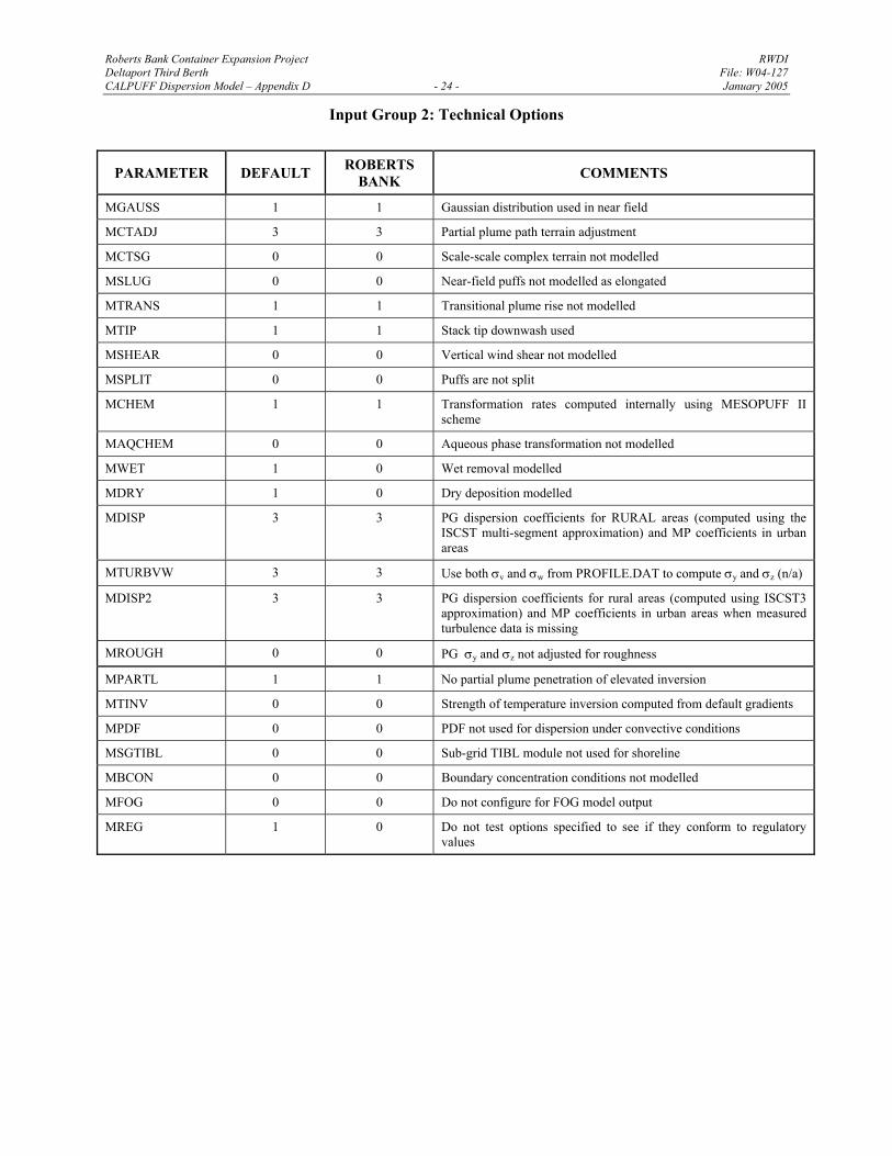
Input Group 2: Technical Options
PARAMETER DEFAULT ROBERTS BANK COMMENTS
MGAUSS 1 1 Gaussian distribution used in near field
MCTADJ 3 3 Partial plume path terrain adjustment
MCTSG 0 0 Scale-scale complex terrain not modelled
MSLUG 0 0 Near-field puffs not modelled as elongated
MTRANS 1 1 Transitional plume rise not modelled
MTIP 1 1 Stack tip downwash used
MSHEAR 0 0 Vertical wind shear not modelled
MSPLIT 0 0 Puffs are not split
MCHEM 1 1 Transformation rates computed internally using MESOPUFF II scheme
MAQCHEM 0 0 Aqueous phase transformation not modelled
MWET 1 0 Wet removal modelled
MDRY 1 0 Dry deposition modelled
MDISP 3 3 PG dispersion coefficients for RURAL areas (computed using the ISCST multi-segment approximation) and MP coefficients in urban areas
MTURBVW 3 3 Use both σv and σw from PROFILE.DAT to compute σy and σz (n/a)
MDISP2 3 3 PG dispersion coefficients for rural areas (computed using ISCST3 approximation) and MP coefficients in urban areas when measured turbulence data is missing
MROUGH 0 0 PG σy and σz not adjusted for roughness
MPARTL 1 1 No partial plume penetration of elevated inversion
MTINV 0 0 Strength of temperature inversion computed from default gradients
MPDF 0 0 PDF not used for dispersion under convective conditions
MSGTIBL 0 0 Sub-grid TIBL module not used for shoreline
MBCON 0 0 Boundary concentration conditions not modelled
MFOG 0 0 Do not configure for FOG model output
MREG 1 0 Do not test options specified to see if they conform to regulatory values
Roberts Bank Container Expansion Project RWDI Deltaport Third Berth File: W04-127 CALPUFF Dispersion Model – Appendix D - 25 - January 2005
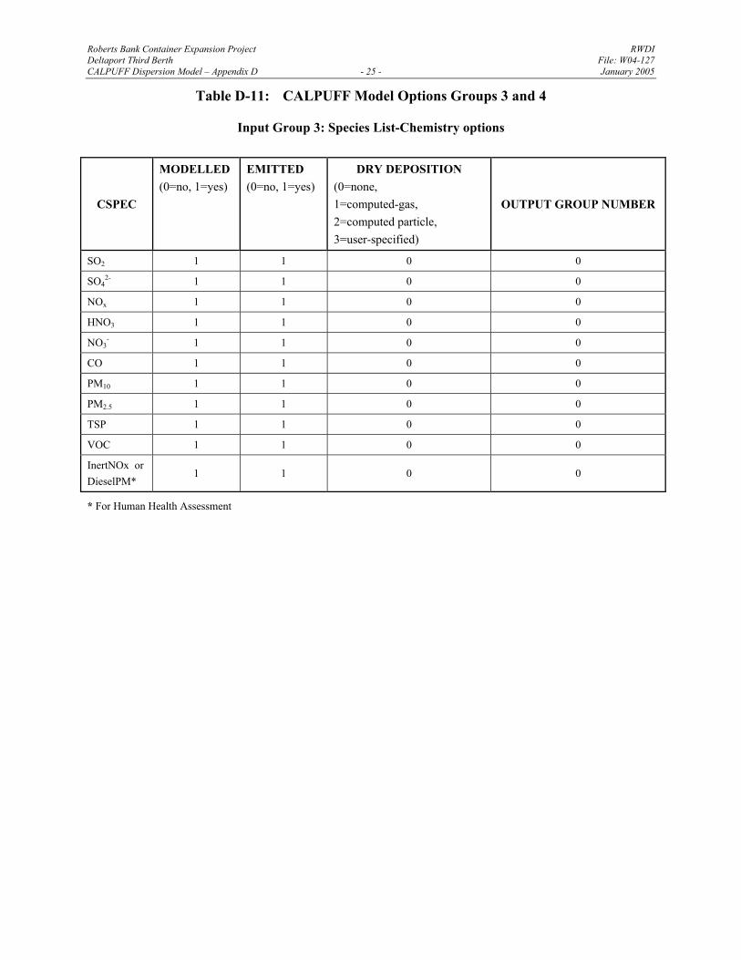
Table D-11: CALPUFF Model Options Groups 3 and 4
Input Group 3: Species List-Chemistry options
CSPEC
MODELLED (0=no, 1=yes)
EMITTED (0=no, 1=yes)
DRY DEPOSITION (0=none, 1=computed-gas, 2=computed particle, 3=user-specified)
OUTPUT GROUP NUMBER
SO2 1 1 0 0
SO42- 1 1 0 0
NOx 1 1 0 0
HNO3 1 1 0 0
NO3- 1 1 0 0
CO 1 1 0 0
PM10 1 1 0 0
PM2.5 1 1 0 0
TSP 1 1 0 0
VOC 1 1 0 0
InertNOx or DieselPM* 1 1 0 0
* For Human Health Assessment
Roberts Bank Container Expansion Project RWDI Deltaport Third Berth File: W04-127 CALPUFF Dispersion Model – Appendix D - 26 - January 2005
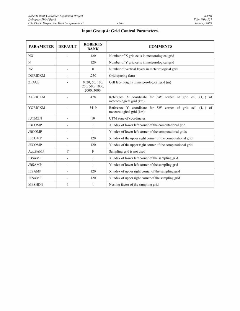
Input Group 4: Grid Control Parameters.
PARAMETER DEFAULT ROBERTS BANK COMMENTS
NX - 120 Number of X grid cells in meteorological grid
N 120 Number of Y grid cells in meteorological grid
NZ - 8 Number of vertical layers in meteorological grid
DGRIDKM - .250 Grid spacing (km)
ZFACE - 0, 20, 50, 100, 250, 500, 1000,
2000, 3000.
Cell face heights in meteorological grid (m)
XORIGKM - 478 Reference X coordinate for SW corner of grid cell (1,1) of meteorological grid (km)
YORIGKM - 5419 Reference Y coordinate for SW corner of grid cell (1,1) of meteorological grid (km)
IUTMZN - 10 UTM zone of coordinates
IBCOMP - 1 X index of lower left corner of the computational grid
JBCOMP - 1 Y index of lower left corner of the computational grids
IECOMP - 120 X index of the upper right corner of the computational grid
JECOMP - 120 Y index of the upper right corner of the computational grid
AqLSAMP T F Sampling grid is not used
IBSAMP - 1 X index of lower left corner of the sampling grid
JBSAMP - 1 Y index of lower left corner of the sampling grid
IESAMP - 120 X index of upper right corner of the sampling grid
JESAMP - 120 Y index of upper right corner of the sampling grid
MESHDN 1 1 Nesting factor of the sampling grid
Roberts Bank Container Expansion Project RWDI Deltaport Third Berth File: W04-127 CALPUFF Dispersion Model – Appendix D - 27 - January 2005
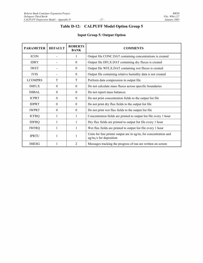
Table D-12: CALPUFF Model Option Group 5
Input Group 5: Output Option
PARAMETER DEFAULT ROBERTS BANK COMMENTS
ICON - 1 Output file CONC.DAT containing concentrations is created
IDRY - 0 Output file DFLX.DAT containing dry fluxes is created
IWET - 0 Output file WFLX.DAT containing wet fluxes is created
IVIS - 0 Output file containing relative humidity data is not created
LCOMPRS T T Perform data compression in output file
IMFLX 0 0 Do not calculate mass fluxes across specific boundaries
IMBAL 0 0 Do not report mass balances
ICPRT 0 0 Do not print concentration fields to the output list file
IDPRT 0 0 Do not print dry flux fields to the output list file
IWPRT 0 0 Do not print wet flux fields to the output list file
ICFRQ 1 1 Concentration fields are printed to output list file every 1 hour
IDFRQ 1 1 Dry flux fields are printed to output list file every 1 hour
IWFRQ 1 1 Wet flux fields are printed to output list file every 1 hour
IPRTU 1 1 Units for line printer output are in ug/m3 for concentration and ug/m2/s for deposition
IMESG 1 2 Messages tracking the progress of run are written on screen
Roberts Bank Container Expansion Project RWDI Deltaport Third Berth File: W04-127 CALPUFF Dispersion Model – Appendix D - 28 - January 2005
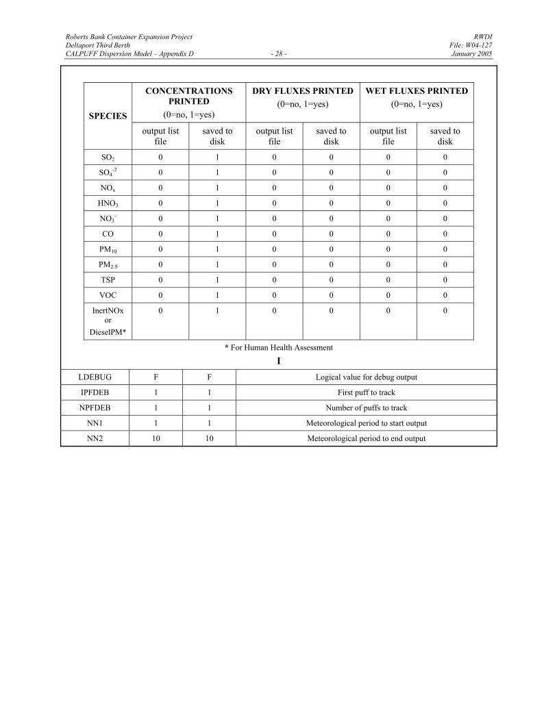
CONCENTRATIONS PRINTED
(0=no, 1=yes)
DRY FLUXES PRINTED (0=no, 1=yes)
WET FLUXES PRINTED (0=no, 1=yes)
SPECIES output list
file saved to
disk output list
file saved to
disk output list
file saved to
disk
SO2 0 1 0 0 0 0
SO4-2 0 1 0 0 0 0
NOx 0 1 0 0 0 0
HNO3 0 1 0 0 0 0
NO3- 0 1 0 0 0 0
CO 0 1 0 0 0 0
PM10 0 1 0 0 0 0
PM2.5 0 1 0 0 0 0
TSP 0 1 0 0 0 0
VOC 0 1 0 0 0 0
InertNOx or
DieselPM*
0 1 0 0 0 0
* For Human Health Assessment
I
LDEBUG F F Logical value for debug output
IPFDEB 1 1 First puff to track
NPFDEB 1 1 Number of puffs to track
NN1 1 1 Meteorological period to start output
NN2 10 10 Meteorological period to end output
Roberts Bank Container Expansion Project RWDI Deltaport Third Berth File: W04-127 CALPUFF Dispersion Model – Appendix D - 29 - January 2005
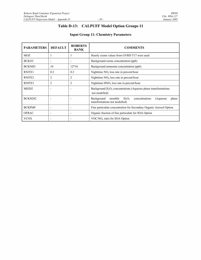
Table D-13: CALPUFF Model Option Groups 11
Input Group 11: Chemistry Parameters
PARAMETERS DEFAULT ROBERTS BANK COMMENTS
MOZ 1 1 Hourly ozone values from GVRD T17 were used
BCKO3 - - Background ozone concentration (ppb)
BCKNH3 10 12*10 Background ammonia concentration (ppb)
RNITE1 0.2 0.2 Nighttime NO2 loss rate in percent/hour
RNITE2 2 2 Nighttime NOX loss rate in percent/hour
RNITE3 2 2 Nighttime HNO3 loss rate in percent/hour
MH202 - - Background H2O2 concentrations (Aqueous phase transformations not modelled)
BCKH202 - - Background monthly H2O2 concentrations (Aqueous phase transformations not modelled)
BCKPMF - - Fine particulate concentration for Secondary Organic Aerosol Option
OFRAC - - Organic fraction of fine particulate for SOA Option
VCNX - - VOC/NOx ratio for SOA Option
Roberts Bank Container Expansion Project RWDI Deltaport Third Berth File: W04-127 CALPUFF Dispersion Model – Appendix D - 30 - January 2005
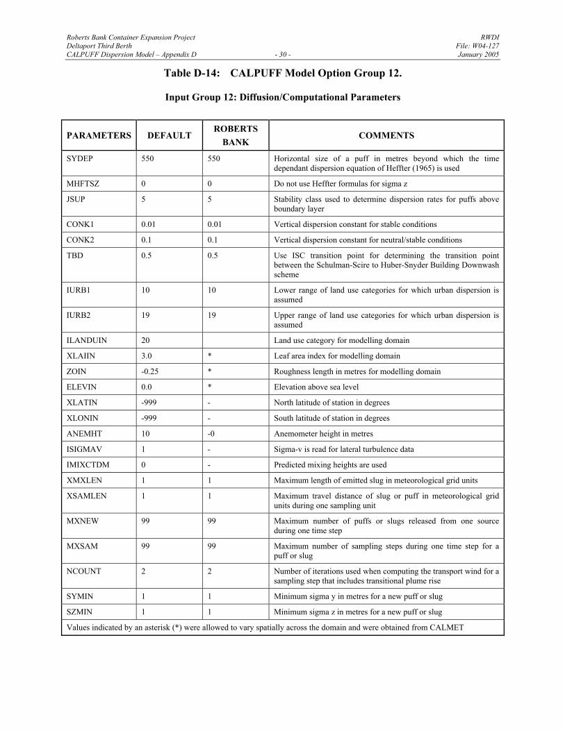
Table D-14: CALPUFF Model Option Group 12.
Input Group 12: Diffusion/Computational Parameters
PARAMETERS DEFAULT ROBERTS
BANK COMMENTS
SYDEP 550 550 Horizontal size of a puff in metres beyond which the time dependant dispersion equation of Heffter (1965) is used
MHFTSZ 0 0 Do not use Heffter formulas for sigma z
JSUP 5 5 Stability class used to determine dispersion rates for puffs above boundary layer
CONK1 0.01 0.01 Vertical dispersion constant for stable conditions
CONK2 0.1 0.1 Vertical dispersion constant for neutral/stable conditions
TBD 0.5 0.5 Use ISC transition point for determining the transition point between the Schulman-Scire to Huber-Snyder Building Downwash scheme
IURB1 10 10 Lower range of land use categories for which urban dispersion is assumed
IURB2 19 19 Upper range of land use categories for which urban dispersion is assumed
ILANDUIN 20 Land use category for modelling domain
XLAIIN 3.0 * Leaf area index for modelling domain
ZOIN -0.25 * Roughness length in metres for modelling domain
ELEVIN 0.0 * Elevation above sea level
XLATIN -999 - North latitude of station in degrees
XLONIN -999 - South latitude of station in degrees
ANEMHT 10 -0 Anemometer height in metres
ISIGMAV 1 - Sigma-v is read for lateral turbulence data
IMIXCTDM 0 - Predicted mixing heights are used
XMXLEN 1 1 Maximum length of emitted slug in meteorological grid units
XSAMLEN 1 1 Maximum travel distance of slug or puff in meteorological grid units during one sampling unit
MXNEW 99 99 Maximum number of puffs or slugs released from one source during one time step
MXSAM 99 99 Maximum number of sampling steps during one time step for a puff or slug
NCOUNT 2 2 Number of iterations used when computing the transport wind for a sampling step that includes transitional plume rise
SYMIN 1 1 Minimum sigma y in metres for a new puff or slug
SZMIN 1 1 Minimum sigma z in metres for a new puff or slug
Values indicated by an asterisk (*) were allowed to vary spatially across the domain and were obtained from CALMET
Roberts Bank Container Expansion Project RWDI Deltaport Third Berth File: W04-127 CALPUFF Dispersion Model – Appendix D - 31 - January 2005
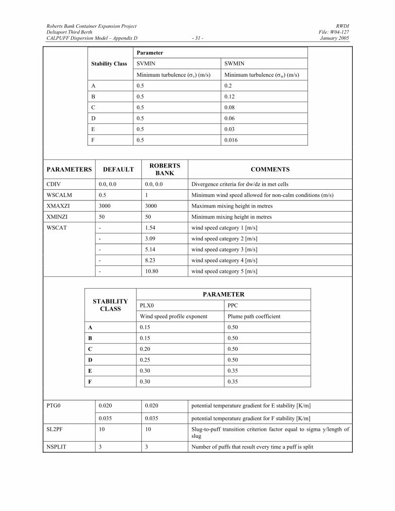
Parameter
SVMIN SWMIN Stability Class
Minimum turbulence (σv) (m/s) Minimum turbulence (σw) (m/s)
A 0.5 0.2
B 0.5 0.12
C 0.5 0.08
D 0.5 0.06
E 0.5 0.03
F 0.5 0.016
PARAMETERS DEFAULT ROBERTS BANK COMMENTS
CDIV 0.0, 0.0 0.0, 0.0 Divergence criteria for dw/dz in met cells
WSCALM 0.5 1 Minimum wind speed allowed for non-calm conditions (m/s)
XMAXZI 3000 3000 Maximum mixing height in metres
XMINZI 50 50 Minimum mixing height in metres
- 1.54 wind speed category 1 [m/s]
- 3.09 wind speed category 2 [m/s]
- 5.14 wind speed category 3 [m/s]
- 8.23 wind speed category 4 [m/s]
WSCAT
- 10.80 wind speed category 5 [m/s]
PARAMETER
PLX0 PPC STABILITY
CLASS Wind speed profile exponent Plume path coefficient
A 0.15 0.50
B 0.15 0.50
C 0.20 0.50
D 0.25 0.50
E 0.30 0.35
F 0.30 0.35
0.020 0.020 potential temperature gradient for E stability [K/m] PTG0
0.035 0.035 potential temperature gradient for F stability [K/m]
SL2PF 10 10 Slug-to-puff transition criterion factor equal to sigma y/length of slug
NSPLIT 3 3 Number of puffs that result every time a puff is split
Roberts Bank Container Expansion Project RWDI Deltaport Third Berth File: W04-127 CALPUFF Dispersion Model – Appendix D - 32 - January 2005
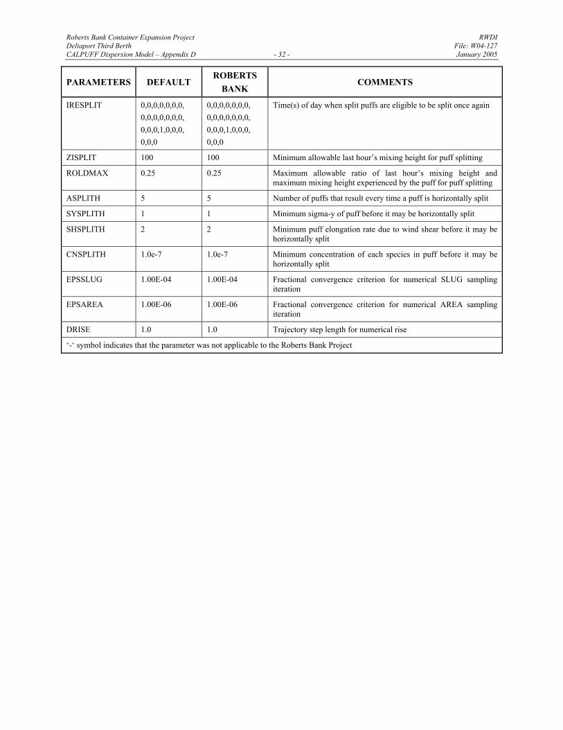
PARAMETERS DEFAULT ROBERTS
BANK COMMENTS
IRESPLIT 0,0,0,0,0,0,0, 0,0,0,0,0,0,0, 0,0,0,1,0,0,0, 0,0,0
0,0,0,0,0,0,0, 0,0,0,0,0,0,0, 0,0,0,1,0,0,0, 0,0,0
Time(s) of day when split puffs are eligible to be split once again
ZISPLIT 100 100 Minimum allowable last hour’s mixing height for puff splitting
ROLDMAX 0.25 0.25 Maximum allowable ratio of last hour’s mixing height and maximum mixing height experienced by the puff for puff splitting
ASPLITH 5 5 Number of puffs that result every time a puff is horizontally split
SYSPLITH 1 1 Minimum sigma-y of puff before it may be horizontally split
SHSPLITH 2 2 Minimum puff elongation rate due to wind shear before it may be horizontally split
CNSPLITH 1.0e-7 1.0e-7 Minimum concentration of each species in puff before it may be horizontally split
EPSSLUG 1.00E-04 1.00E-04 Fractional convergence criterion for numerical SLUG sampling iteration
EPSAREA 1.00E-06 1.00E-06 Fractional convergence criterion for numerical AREA sampling iteration
DRISE 1.0 1.0 Trajectory step length for numerical rise
‘-‘ symbol indicates that the parameter was not applicable to the Roberts Bank Project
Roberts Bank Container Expansion Project RWDI Deltaport Third Berth File: W04-127 CALPUFF Dispersion Model – Appendix D - 33 - January 2005
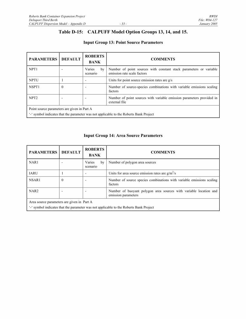
Table D-15: CALPUFF Model Option Groups 13, 14, and 15.
Input Group 13: Point Source Parameters
PARAMETERS DEFAULT ROBERTS
BANK COMMENTS
NPT1 - Varies by scenario
Number of point sources with constant stack parameters or variable emission rate scale factors
NPTU 1 - Units for point source emission rates are g/s
NSPT1 0 - Number of source-species combinations with variable emissions scaling factors
NPT2 - - Number of point sources with variable emission parameters provided in external file
Point source parameters are given in Part A ‘-‘ symbol indicates that the parameter was not applicable to the Roberts Bank Project
Input Group 14: Area Source Parameters
PARAMETERS DEFAULT ROBERTS
BANK COMMENTS
NAR1 - Varies by scenario
Number of polygon area sources
IARU 1 - Units for area source emission rates are g/m2/s
NSAR1 0 - Number of source species combinations with variable emissions scaling factors
NAR2 - - Number of buoyant polygon area sources with variable location and emission parameters
Area source parameters are given in Part A ‘-‘ symbol indicates that the parameter was not applicable to the Roberts Bank Project
Roberts Bank Container Expansion Project RWDI Deltaport Third Berth File: W04-127 CALPUFF Dispersion Model – Appendix D - 34 - January 2005
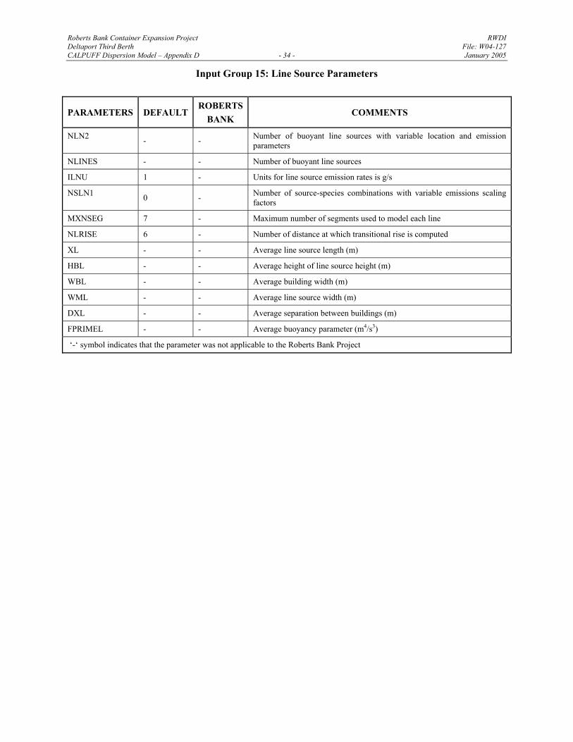
Input Group 15: Line Source Parameters
PARAMETERS DEFAULT ROBERTS
BANK COMMENTS
NLN2 - - Number of buoyant line sources with variable location and emission parameters
NLINES - - Number of buoyant line sources
ILNU 1 - Units for line source emission rates is g/s
NSLN1 0 - Number of source-species combinations with variable emissions scaling factors
MXNSEG 7 - Maximum number of segments used to model each line
NLRISE 6 - Number of distance at which transitional rise is computed
XL - - Average line source length (m)
HBL - - Average height of line source height (m)
WBL - - Average building width (m)
WML - - Average line source width (m)
DXL - - Average separation between buildings (m)
FPRIMEL - - Average buoyancy parameter (m4/s3)
‘-‘ symbol indicates that the parameter was not applicable to the Roberts Bank Project
Roberts Bank Container Expansion Project RWDI Deltaport Third Berth File: W04-127 CALPUFF Dispersion Model – Appendix D - 35 - January 2005
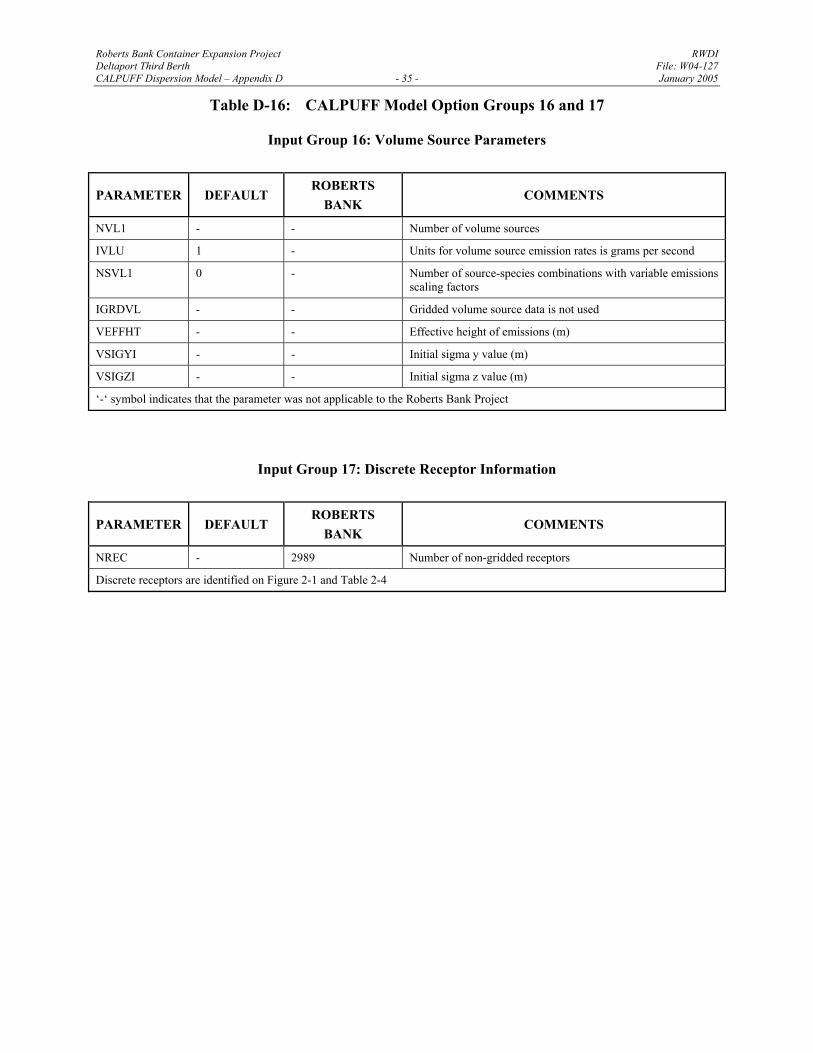
Table D-16: CALPUFF Model Option Groups 16 and 17
Input Group 16: Volume Source Parameters
PARAMETER DEFAULT ROBERTS
BANK COMMENTS
NVL1 - - Number of volume sources
IVLU 1 - Units for volume source emission rates is grams per second
NSVL1 0 - Number of source-species combinations with variable emissions scaling factors
IGRDVL - - Gridded volume source data is not used
VEFFHT - - Effective height of emissions (m)
VSIGYI - - Initial sigma y value (m)
VSIGZI - - Initial sigma z value (m)
‘-‘ symbol indicates that the parameter was not applicable to the Roberts Bank Project
Input Group 17: Discrete Receptor Information
PARAMETER DEFAULT ROBERTS
BANK COMMENTS
NREC - 2989 Number of non-gridded receptors
Discrete receptors are identified on Figure 2-1 and Table 2-4
Roberts Bank Container Expansion Project RWDI Deltaport Third Berth File: W04-127 CALPUFF Dispersion Model – Appendix D - 36 - January 2005
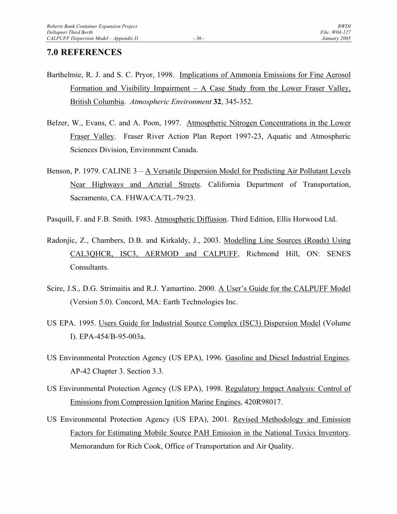
7.0 REFERENCES
Barthelmie, R. J. and S. C. Pryor, 1998. Implications of Ammonia Emissions for Fine Aerosol
Formation and Visibility Impairment – A Case Study from the Lower Fraser Valley,
British Columbia. Atmospheric Environment 32, 345-352.
Belzer, W., Evans, C. and A. Poon, 1997. Atmospheric Nitrogen Concentrations in the Lower
Fraser Valley. Fraser River Action Plan Report 1997-23, Aquatic and Atmospheric
Sciences Division, Environment Canada.
Benson, P. 1979. CALINE 3 – A Versatile Dispersion Model for Predicting Air Pollutant Levels
Near Highways and Arterial Streets. California Department of Transportation,
Sacramento, CA. FHWA/CA/TL-79/23.
Pasquill, F. and F.B. Smith. 1983. Atmospheric Diffusion. Third Edition, Ellis Horwood Ltd.
Radonjic, Z., Chambers, D.B. and Kirkaldy, J., 2003. Modelling Line Sources (Roads) Using
CAL3QHCR, ISC3, AERMOD and CALPUFF, Richmond Hill, ON: SENES
Consultants.
Scire, J.S., D.G. Strimaitis and R.J. Yamartino. 2000. A User’s Guide for the CALPUFF Model
(Version 5.0). Concord, MA: Earth Technologies Inc.
US EPA. 1995. Users Guide for Industrial Source Complex (ISC3) Dispersion Model (Volume
I). EPA-454/B-95-003a.
US Environmental Protection Agency (US EPA), 1996. Gasoline and Diesel Industrial Engines.
AP-42 Chapter 3. Section 3.3.
US Environmental Protection Agency (US EPA), 1998. Regulatory Impact Analysis: Control of
Emissions from Compression Ignition Marine Engines, 420R98017.
US Environmental Protection Agency (US EPA), 2001. Revised Methodology and Emission
Factors for Estimating Mobile Source PAH Emission in the National Toxics Inventory.
Memorandum for Rich Cook, Office of Transportation and Air Quality.
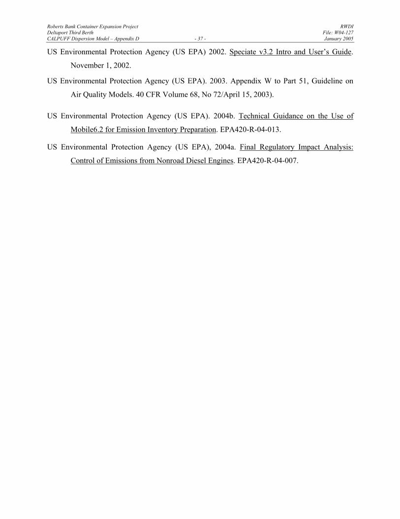
Roberts Bank Container Expansion Project RWDI Deltaport Third Berth File: W04-127 CALPUFF Dispersion Model – Appendix D - 37 - January 2005
US Environmental Protection Agency (US EPA) 2002. Speciate v3.2 Intro and User’s Guide.
November 1, 2002.
US Environmental Protection Agency (US EPA). 2003. Appendix W to Part 51, Guideline on
Air Quality Models. 40 CFR Volume 68, No 72/April 15, 2003).
US Environmental Protection Agency (US EPA). 2004b. Technical Guidance on the Use of
Mobile6.2 for Emission Inventory Preparation. EPA420-R-04-013.
US Environmental Protection Agency (US EPA), 2004a. Final Regulatory Impact Analysis:
Control of Emissions from Nonroad Diesel Engines. EPA420-R-04-007.