Appendix E1

CALPUFF Dispersion Modeling of Ocean-Going Vessels Emissions

This page is intentionally blank.

E1-1

CALPUFF Dispersion Modeling of Ocean-Going Vessels Emissions

Prepared by:

Atmospheric Modeling and Support Section Modeling and Meteorology Branch

Planning and Technical Support Division

May 2008

E1-2

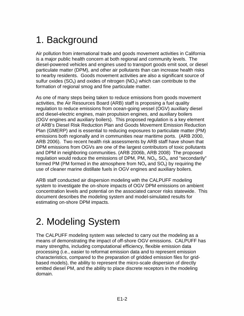
1. Background Air pollution from international trade and goods movement activities in California is a major public health concern at both regional and community levels. The diesel-powered vehicles and engines used to transport goods emit soot, or diesel particulate matter (DPM), and other air pollutants than can increase health risks to nearby residents. Goods movement activities are also a significant source of sulfur oxides (SOx) and oxides of nitrogen (NOx) which can contribute to the formation of regional smog and fine particulate matter. As one of many steps being taken to reduce emissions from goods movement activities, the Air Resources Board (ARB) staff is proposing a fuel quality regulation to reduce emissions from ocean-going vessel (OGV) auxiliary diesel and diesel-electric engines, main propulsion engines, and auxiliary boilers (OGV engines and auxiliary boilers). This proposed regulation is a key element of ARB’s Diesel Risk Reduction Plan and Goods Movement Emission Reduction Plan (GMERP) and is essential to reducing exposures to particulate matter (PM) emissions both regionally and in communities near maritime ports. (ARB 2000, ARB 2006). Two recent health risk assessments by ARB staff have shown that DPM emissions from OGVs are one of the largest contributors of toxic pollutants and DPM in neighboring communities. (ARB 2006b, ARB 2008) The proposed regulation would reduce the emissions of DPM, PM, NOx, SOx, and “secondarily” formed PM (PM formed in the atmosphere from NOx and SOx) by requiring the use of cleaner marine distillate fuels in OGV engines and auxiliary boilers. ARB staff conducted air dispersion modeling with the CALPUFF modeling system to investigate the on-shore impacts of OGV DPM emissions on ambient concentration levels and potential on the associated cancer risks statewide. This document describes the modeling system and model-simulated results for estimating on-shore DPM impacts.

2. Modeling System The CALPUFF modeling system was selected to carry out the modeling as a means of demonstrating the impact of off-shore OGV emissions. CALPUFF has many strengths, including computational efficiency, flexible emission data processing (i.e., easier to reformat emission data and to represent emission characteristics, compared to the preparation of gridded emission files for grid-based models), the ability to represent the micro-scale dispersion of directly emitted diesel PM, and the ability to place discrete receptors in the modeling domain.

E1-3

At the time that ARB staff started this modeling exercise, the then official USEPA-approved version was used. The modeling system was publicly available on USEPA’s website:

http://www.epa.gov/scram001/dispersion_prefrec.htm#calpuff

The USEPA recommended the following version/level of the meteorological pre-processor (CALMET), dispersion model (CALPUFF) and post-processor (CALPOST):

• CALPUFF - Version 5.711a - July 16, 2004 • CALMET - Version 5.53a - July 16, 2004 • CALPOST - Version 5.51 - July 9, 2003

2.1 CALMET

CALMET is a diagnostic meteorological model. It has been under constant update and improvement by the developer (Scire, 2000).

CALMET uses a two-step approach to calculate wind fields. In the first step, an initial-guess wind field is adjusted for slope flows and terrain blocking effects using terrain data to produce a secondary wind field. The initial guess wind fields used for this project are based on 12-km resolution MM5 meteorological fields for 2002 . In the second step, an objective analysis, based on the adjusted MM5 (initial guess) meteorology, is performed on observational data to produce a final uniform, 3-dimensional, observation-based wind field at all grid points.

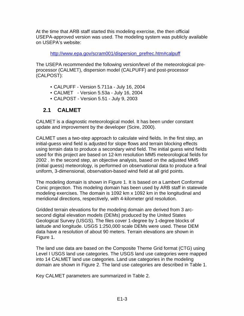
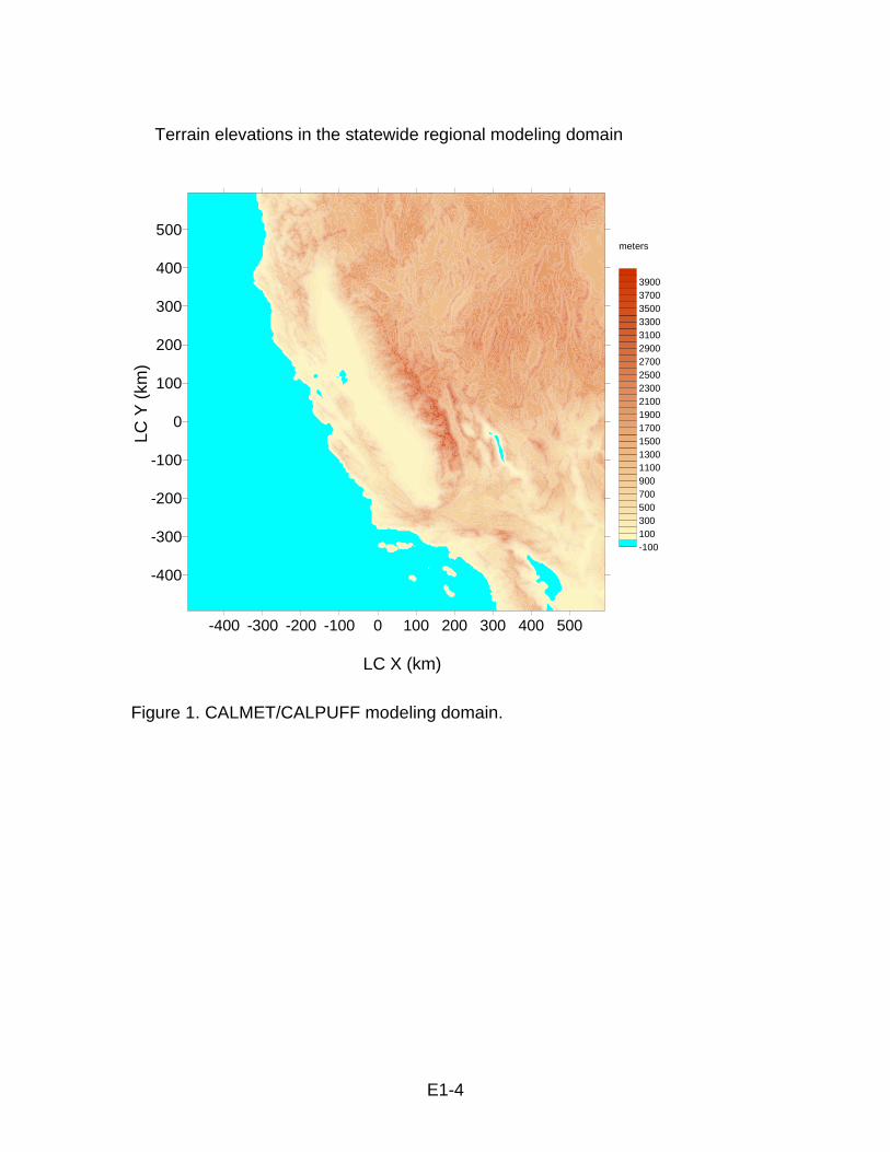
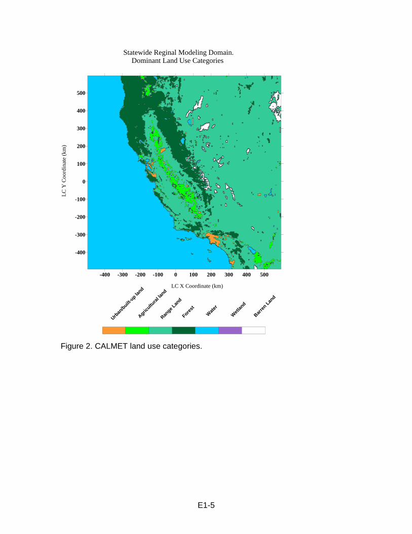
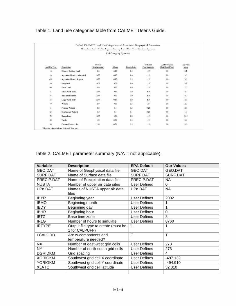
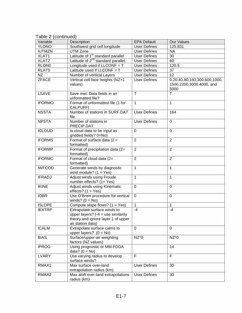
The modeling domain is shown in Figure 1. It is based on a Lambert Conformal Conic projection. This modeling domain has been used by ARB staff in statewide modeling exercises. The domain is 1092 km x 1092 km in the longitudinal and meridional directions, respectively, with 4-kilometer grid resolution. Gridded terrain elevations for the modeling domain are derived from 3 arc-second digital elevation models (DEMs) produced by the United States Geological Survey (USGS). The files cover 1-degree by 1-degree blocks of latitude and longitude. USGS 1:250,000 scale DEMs were used. These DEM data have a resolution of about 90 meters. Terrain elevations are shown in Figure 1. The land use data are based on the Composite Theme Grid format (CTG) using Level I USGS land use categories. The USGS land use categories were mapped into 14 CALMET land use categories. Land use categories in the modeling domain are shown in Figure 2. The land use categories are described in Table 1. Key CALMET parameters are summarized in Table 2.

E1-4

-400 -300 -200 -100 0 100 200 300 400 500

-400

-300

-200

-100

0

100

200

300

400

500

-100100300500700900110013001500170019002100230025002700290031003300350037003900

Terrain elevations in the statewide regional modeling domain

LC X (km)

meters

LC Y

(km

)

Figure 1. CALMET/CALPUFF modeling domain.

E1-5

-400 -300 -200 -100 0 100 200 300 400 500

-400

-300

-200

-100

0

100

200

300

400

500

1 2 3 4 5 6 7

Statewide Reginal Modeling Domain.Dominant Land Use Categories

Urban

/built

-up la

nd

Agricultu

ral la

nd

Forest

Wat

er

Wet

land

Barre

n Lan

d

LC X Coordinate (km)

LC

Y C

oord

inat

e (k

m)

Range L

and

Figure 2. CALMET land use categories.

E1-6

Table 1. Land use categories table from CALMET User's Guide.

Table 2. CALMET parameter summary (N/A = not applicable).

Variable Description EPA Default Our Values GEO.DAT Name of Geophysical data file GEO.DAT GEO.DAT SURF.DAT Name of Surface data file SURF.DAT SURF.DAT PRECIP.DAT Name of Precipitation data file PRECIP.DAT NA NUSTA Number of upper air data sites User Defined 0 UPn.DAT Names of NUSTA upper air data

files UPn.DAT NA

IBYR Beginning year User Defines 2002 IBMO Beginning month User Defines 1 IBDY Beginning day User Defines 1 IBHR Beginning hour User Defines 0 IBTZ Base time zone User Defines 8 IRLG Number of hours to simulate User Defines 8760 IRTYPE Output file type to create (must be

1 for CALPUFF) 1 1

LCALGRD Are w-components and temperature needed?

T T

NX Number of east-west grid cells User Defines 273 NY Number of north-south grid cells User Defines 273 DGRIDKM Grid spacing User Defines 4 XORIGKM Southwest grid cell X coordinate User Defines -497.132 YORIGKM Southwest grid cell Y coordinate User Defines -494.910 XLATO Southwest grid cell latitude User Defines 32.310

E1-7

Table 2 (continued) Variable Description EPA Default Our Values YLONO Southwest grid cell longitude User Defines 125.831 IUTMZN UTM Zone User Defines NA XLAT1 Latitude of 1st standard parallel User Defines 30 XLAT2 Latitude of 2nd standard parallel User Defines 60 RLON0 Longitude used if LLCONF = T User Defines 120.5 RLAT0 Latitude used if LLCONF = T User Defines 37 NZ Number of vertical Layers User Defines 12 ZFACE Vertical cell face heights (NZ+1

values) User Defines 0,20,40,80,160,300,600,1000,

1500,2200,3000,4000, and 5000

LSAVE Save met. Data fields in an unformatted file?

T T

IFORMO Format of unformatted file (1 for CALPUFF)

1 1

NSSTA Number of stations in SURF.DAT file

User Defines 164

NPSTA Number of stations in PRECIP.DAT

User Defines 0

ICLOUD Is cloud data to be input as gridded fields? 0=No)

0 0

IFORMS Format of surface data (2 = formatted)

2 2

IFORMP Format of precipitation data (2= formatted)

2 2

IFORMC Format of cloud data (2= formatted)

2 2

IWFCOD Generate winds by diagnostic wind module? (1 = Yes)

1 1

IFRADJ Adjust winds using Froude number effects? (1= Yes)

1 1

IKINE Adjust winds using Kinematic effects? (1 = Yes)

0 0

IOBR Use O’Brien procedure for vertical winds? (0 = No)

0 0

ISLOPE Compute slope flows? (1 = Yes) 1 1 IEXTRP Extrapolate surface winds to

upper layers? (-4 = use similarity theory and ignore layer 1 of upper air station data)

-4 -4

ICALM Extrapolate surface calms to upper layers? (0 = No)

0 0

BIAS Surface/upper-air weighting factors (NZ values)

NZ*0 NZ*0

IPROG Using prognostic or MM-FDDA data? (0 = No)

14

LVARY Use varying radius to develop surface winds?

F F

RMAX1 Max surface over-land extrapolation radius (km)

User Defines 30

RMAX2 Max aloft over-land extrapolations radius (km)

User Defines 30

E1-8

Table 2 (continued) Variable Description EPA Default Our Values RMAX3 Maximum over-water

extrapolation radius (km) User Defines 50

RMIN Minimum extrapolation radius (km)

0.1 0.1

RMIN2 Distance (km) around an upper air site where vertical extrapolation is excluded (Set to –1 if IEXTRP = ±4)

4 4

TERRAD Radius of influence of terrain features (km)

User Defines 50

R1 Relative weight at surface of Step 1 field and obs

User Defines 1.0

R2 Relative weight aloft of Step 1 field and obs

User Defines 1.0

DIVLIM Maximum acceptable divergence 5.E-6 5.E-6 NITER Max number of passes in

divergence minimization 50 50

NSMTH Number of passes in smoothing (NZ values)

2,4*(NZ-1) 2,4*(NZ-1)

NINTR2 Max number of stations for interpolations (NA values)

99 99

CRITFN Critical Froude number 1 1 ALPHA Empirical factor triggering

kinematic effects 0.1 0.1

IDIOPT1 Compute temperatures from observations (0 = True)

0 0

ISURFT Surface station to use for surface temperature (between 1 and NSSTA)

User Defines 1

IDIOPT2 Compute domain-average lapse rates? (0 = True)

0 0

IUPT Station for lapse rates (between 1 and NUSTA)

User Defines NA

ZUPT Depth of domain-average lapse rate (m)

200 200

IDIOPT3 Compute internally initial guess winds? (0 = True)

0 0

IUPWND Upper air station for domain winds (-1 = 1/r**2 interpolation of all stations)

-1 -1

ZUPWND Bottom and top of layer for 1st guess winds (m)

1,1000 1,1000

IDIOPT4 Read surface winds from SURF.DAT? ( 0 = True)

0 0

IDIOPT5 Read aloft winds from UPn.DAT? ( 0 = True)

0 0

CONSTB Neutral mixing height B constant 1.41 1.41 CONSTE Convective mixing height E

constant 0.15 0.15

CONSTN Stable mixing height N constant 2400 2400

E1-9

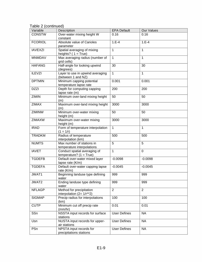
Table 2 (continued) Variable Description EPA Default Our Values CONSTW Over-water mixing height W

constant 0.16 0.16

FCORIOL Absolute value of Carioles parameter

1.E-4 1.E-4

IAVEXZI Spatial averaging of mixing heights? ( 1 = True)

1 1

MNMDAV Max averaging radius (number of grid cells)

1 1

HAFANG Half-angle for looking upwind (degrees)

30 30

ILEVZI Layer to use in upwind averaging (between 1 and NZ)

1 1

DPTMIN Minimum capping potential temperature lapse rate

0.001 0.001

DZZI Depth for computing capping lapse rate (m)

200 200

ZIMIN Minimum over-land mixing height (m)

50 50

ZIMAX Maximum over-land mixing height (m)

3000 3000

ZIMINW Minimum over-water mixing height (m)

50 50

ZIMAXW Maximum over-water mixing height (m)

3000 3000

IRAD Form of temperature interpolation (1 = 1/r)

1 1

TRADKM Radius of temperature interpolation (km)

500 500

NUMTS Max number of stations in temperature interpolations

5 5

IAVET Conduct spatial averaging of temperature? (1 = True)

1 0

TGDEFB Default over-water mixed layer lapse rate (K/m)

-0.0098 -0.0098

TGDEFA Default over-water capping lapse rate (K/m)

-0.0045 -0.0045

JWAT1 Beginning landuse type defining water

999 999

JWAT2 Ending landuse type defining water

999 999

NFLAGP Method for precipitation interpolation (2= 1/r**2)

2 2

SIGMAP Precip radius for interpolations (km)

100 100

CUTP Minimum cut off precip rate (mm/hr)

0.01 0.01

SSn NSSTA input records for surface stations

User Defines NA

Usn NUSTA input records for upper-air stations

User Defines NA

PSn NPSTA input records for precipitations stations

User Defines NA

E1-10

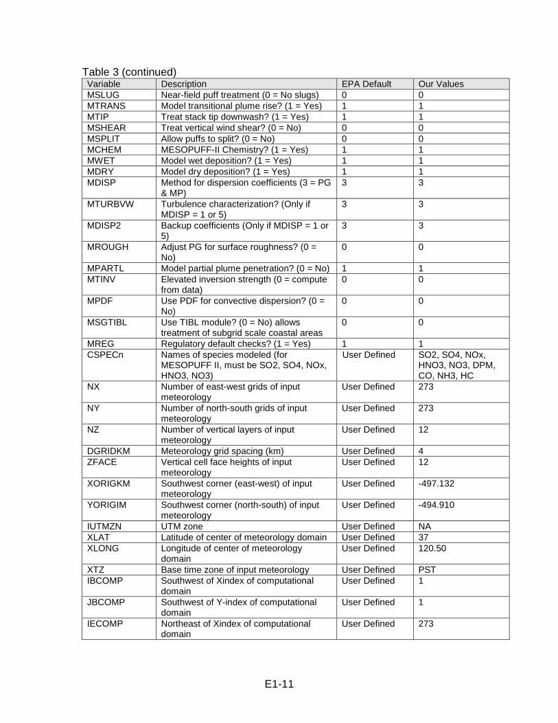
2.2 CALPUFF CALPUFF is a multi-layer, multi-species non-steady-state Gaussian puff dispersion model which can simulate the effects of time- and space-varying meteorological conditions on pollutant transport, transformation, and removal. CALPUFF contains algorithms for near-source effects such as building downwash, transitional plume rise, subgrid scale terrain interactions as well as longer range effects such as pollutant removal (wet scavenging and dry deposition), chemical transformation, vertical wind shear, overwater transport and coastal interaction effects. The CALPUFF modeling domain is identical to the CALMET modeling domain. Key CALPUFF settings are summarized in Table 3. Table 3. CALPUFF parameter summary. Variable Description EPA Default Our Values METDAT CALMET input data filename CALMET.DAT CALMET.DAT PUFLST Filename for general output from

CALPUFF CALPUFF.LST CALPUFF.LST

CONDAT Filename for output concentration data CONC.DAT CONC.DAT DFDAT Filename for output dry deposition fluxes DFLX.DAT DFLX.DAT WFDAT Filename for output wet deposition fluxes WFLX.DAT WFLX.DAT VISDAT Filename for output relative humidities (for

visibility) VISB.DAT VISB.DAT

METRUN Do we run all periods (1) or a subset (0)? 0 0 IBYR Beginning year User Defined 2002 IBMO Beginning month User Defined 1 IBDY Beginning day User Defined 1 IBHR Beginning hour User Defined 0 IRLG Length of runs (hours) User Defined 8760 NSPEC Number of species modeled (for

MESOPUFF II chemistry) User Defined 6

NSE Number of species emitted 3 3 MRESTART Restart options (0 = no restart), allows

splitting runs into smaller segments 0 1

METFM Format of input meteorology (1 = CALMET)

1 1

AVET Averaging time lateral dispersion parameters (minutes)

60 60

MGAUSS Near-field vertical distribution (1 = Gaussian)

1 1

MCTADJ Terrain adjustments to plume path (3 = Plume path)

3 3

MCTSG Do we have subgrid hills? (0 = No), allows CTDM-like treatment for subgrid scale hills

0 0

E1-11

Table 3 (continued) Variable Description EPA Default Our Values MSLUG Near-field puff treatment (0 = No slugs) 0 0 MTRANS Model transitional plume rise? (1 = Yes) 1 1 MTIP Treat stack tip downwash? (1 = Yes) 1 1 MSHEAR Treat vertical wind shear? (0 = No) 0 0 MSPLIT Allow puffs to split? (0 = No) 0 0 MCHEM MESOPUFF-II Chemistry? (1 = Yes) 1 1 MWET Model wet deposition? (1 = Yes) 1 1 MDRY Model dry deposition? (1 = Yes) 1 1 MDISP Method for dispersion coefficients (3 = PG

& MP) 3 3

MTURBVW Turbulence characterization? (Only if MDISP = 1 or 5)

3 3

MDISP2 Backup coefficients (Only if MDISP = 1 or 5)

3 3

MROUGH Adjust PG for surface roughness? (0 = No)

0 0

MPARTL Model partial plume penetration? (0 = No) 1 1 MTINV Elevated inversion strength (0 = compute

from data) 0 0

MPDF Use PDF for convective dispersion? (0 = No)

0 0

MSGTIBL Use TIBL module? (0 = No) allows treatment of subgrid scale coastal areas

0 0

MREG Regulatory default checks? (1 = Yes) 1 1 CSPECn Names of species modeled (for

MESOPUFF II, must be SO2, SO4, NOx, HNO3, NO3)

User Defined SO2, SO4, NOx, HNO3, NO3, DPM, CO, NH3, HC

NX Number of east-west grids of input meteorology

User Defined 273

NY Number of north-south grids of input meteorology

User Defined 273

NZ Number of vertical layers of input meteorology

User Defined 12

DGRIDKM Meteorology grid spacing (km) User Defined 4 ZFACE Vertical cell face heights of input

meteorology User Defined 12

XORIGKM Southwest corner (east-west) of input meteorology

User Defined -497.132

YORIGIM Southwest corner (north-south) of input meteorology

User Defined -494.910

IUTMZN UTM zone User Defined NA XLAT Latitude of center of meteorology domain User Defined 37 XLONG Longitude of center of meteorology

domain User Defined 120.50

XTZ Base time zone of input meteorology User Defined PST IBCOMP Southwest of Xindex of computational

domain User Defined 1

JBCOMP Southwest of Y-index of computational domain

User Defined 1

IECOMP Northeast of Xindex of computational domain

User Defined 273

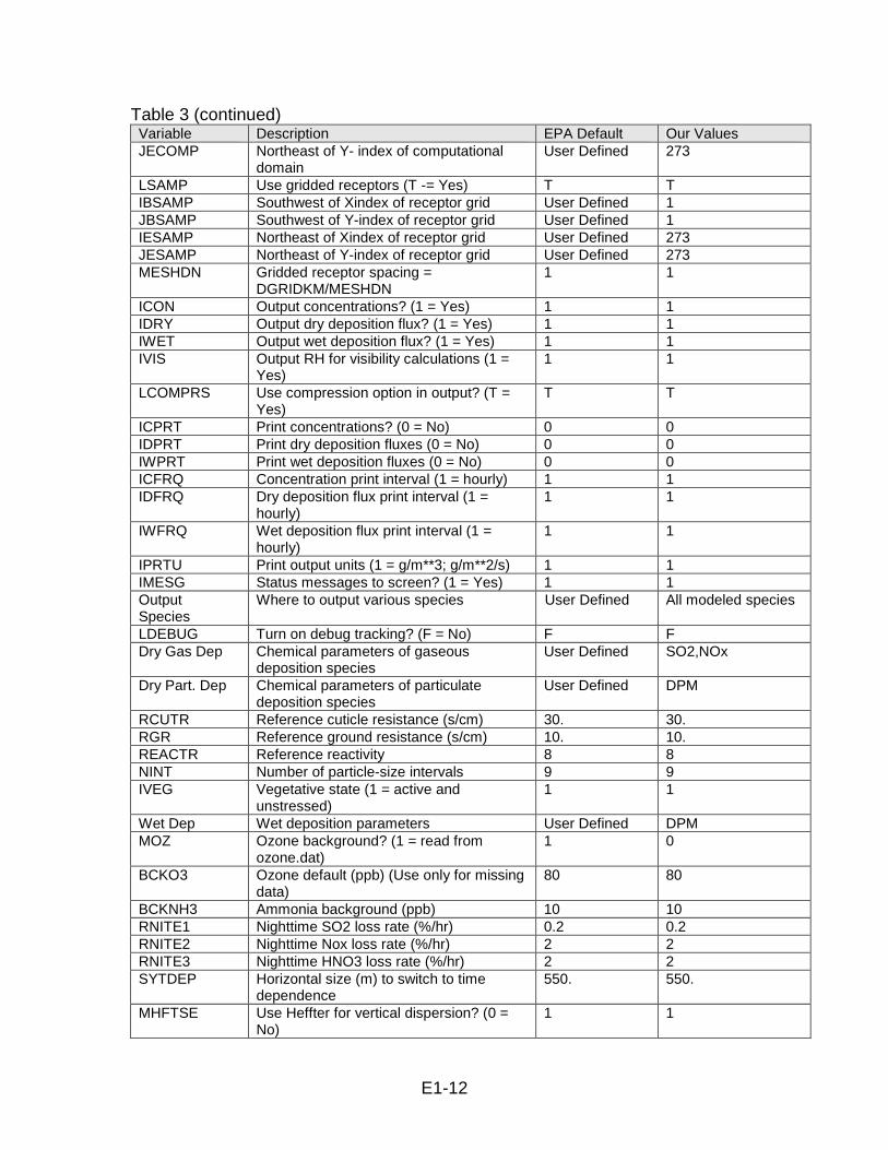
E1-12

Table 3 (continued) Variable Description EPA Default Our Values JECOMP Northeast of Y- index of computational

domain User Defined 273

LSAMP Use gridded receptors (T -= Yes) T T IBSAMP Southwest of Xindex of receptor grid User Defined 1 JBSAMP Southwest of Y-index of receptor grid User Defined 1 IESAMP Northeast of Xindex of receptor grid User Defined 273 JESAMP Northeast of Y-index of receptor grid User Defined 273 MESHDN Gridded receptor spacing =

DGRIDKM/MESHDN 1 1

ICON Output concentrations? (1 = Yes) 1 1 IDRY Output dry deposition flux? (1 = Yes) 1 1 IWET Output wet deposition flux? (1 = Yes) 1 1 IVIS Output RH for visibility calculations (1 =

Yes) 1 1

LCOMPRS Use compression option in output? (T = Yes)

T T

ICPRT Print concentrations? (0 = No) 0 0 IDPRT Print dry deposition fluxes (0 = No) 0 0 IWPRT Print wet deposition fluxes (0 = No) 0 0 ICFRQ Concentration print interval (1 = hourly) 1 1 IDFRQ Dry deposition flux print interval (1 =

hourly) 1 1

IWFRQ Wet deposition flux print interval (1 = hourly)

1 1

IPRTU Print output units (1 = g/m**3; g/m**2/s) 1 1 IMESG Status messages to screen? (1 = Yes) 1 1 Output Species

Where to output various species User Defined All modeled species

LDEBUG Turn on debug tracking? (F = No) F F Dry Gas Dep Chemical parameters of gaseous

deposition species User Defined SO2,NOx

Dry Part. Dep Chemical parameters of particulate deposition species

User Defined DPM

RCUTR Reference cuticle resistance (s/cm) 30. 30. RGR Reference ground resistance (s/cm) 10. 10. REACTR Reference reactivity 8 8 NINT Number of particle-size intervals 9 9 IVEG Vegetative state (1 = active and

unstressed) 1 1

Wet Dep Wet deposition parameters User Defined DPM MOZ Ozone background? (1 = read from

ozone.dat) 1 0

BCKO3 Ozone default (ppb) (Use only for missing data)

80 80

BCKNH3 Ammonia background (ppb) 10 10 RNITE1 Nighttime SO2 loss rate (%/hr) 0.2 0.2 RNITE2 Nighttime Nox loss rate (%/hr) 2 2 RNITE3 Nighttime HNO3 loss rate (%/hr) 2 2 SYTDEP Horizontal size (m) to switch to time

dependence 550. 550.

MHFTSE Use Heffter for vertical dispersion? (0 =

No) 1 1

E1-13

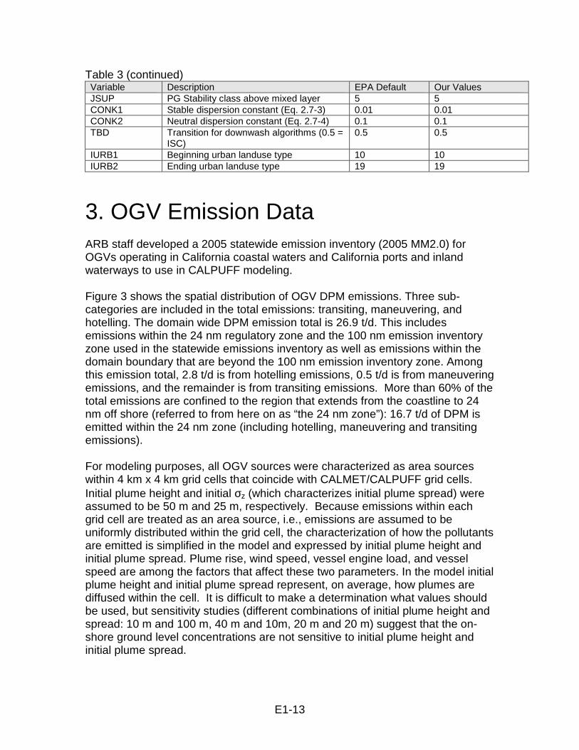
Table 3 (continued) Variable Description EPA Default Our Values JSUP PG Stability class above mixed layer 5 5 CONK1 Stable dispersion constant (Eq. 2.7-3) 0.01 0.01 CONK2 Neutral dispersion constant (Eq. 2.7-4) 0.1 0.1 TBD Transition for downwash algorithms (0.5 =

ISC) 0.5 0.5

IURB1 Beginning urban landuse type 10 10 IURB2 Ending urban landuse type 19 19

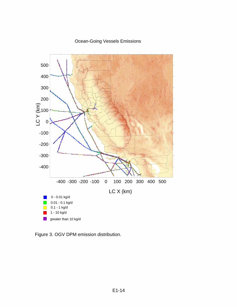
3. OGV Emission Data ARB staff developed a 2005 statewide emission inventory (2005 MM2.0) for OGVs operating in California coastal waters and California ports and inland waterways to use in CALPUFF modeling. Figure 3 shows the spatial distribution of OGV DPM emissions. Three sub-categories are included in the total emissions: transiting, maneuvering, and hotelling. The domain wide DPM emission total is 26.9 t/d. This includes emissions within the 24 nm regulatory zone and the 100 nm emission inventory zone used in the statewide emissions inventory as well as emissions within the domain boundary that are beyond the 100 nm emission inventory zone. Among this emission total, 2.8 t/d is from hotelling emissions, 0.5 t/d is from maneuvering emissions, and the remainder is from transiting emissions. More than 60% of the total emissions are confined to the region that extends from the coastline to 24 nm off shore (referred to from here on as “the 24 nm zone”): 16.7 t/d of DPM is emitted within the 24 nm zone (including hotelling, maneuvering and transiting emissions). For modeling purposes, all OGV sources were characterized as area sources within 4 km x 4 km grid cells that coincide with CALMET/CALPUFF grid cells. Initial plume height and initial σz (which characterizes initial plume spread) were assumed to be 50 m and 25 m, respectively. Because emissions within each grid cell are treated as an area source, i.e., emissions are assumed to be uniformly distributed within the grid cell, the characterization of how the pollutants are emitted is simplified in the model and expressed by initial plume height and initial plume spread. Plume rise, wind speed, vessel engine load, and vessel speed are among the factors that affect these two parameters. In the model initial plume height and initial plume spread represent, on average, how plumes are diffused within the cell. It is difficult to make a determination what values should be used, but sensitivity studies (different combinations of initial plume height and spread: 10 m and 100 m, 40 m and 10m, 20 m and 20 m) suggest that the on-shore ground level concentrations are not sensitive to initial plume height and initial plume spread.

E1-14

Ocean-Going Vessels Emissions

-400 -300 -200 -100 0 100 200 300 400 500

-400

-300

-200

-100

0

100

200

300

400

500

LC X (km)

LC Y

(km

)

0 - 0.01 kg/d

0.01 - 0.1 kg/d

1 - 10 kg/d

greater than 10 kg/d

0.1 - 1 kg/d

Figure 3. OGV DPM emission distribution.

E1-15

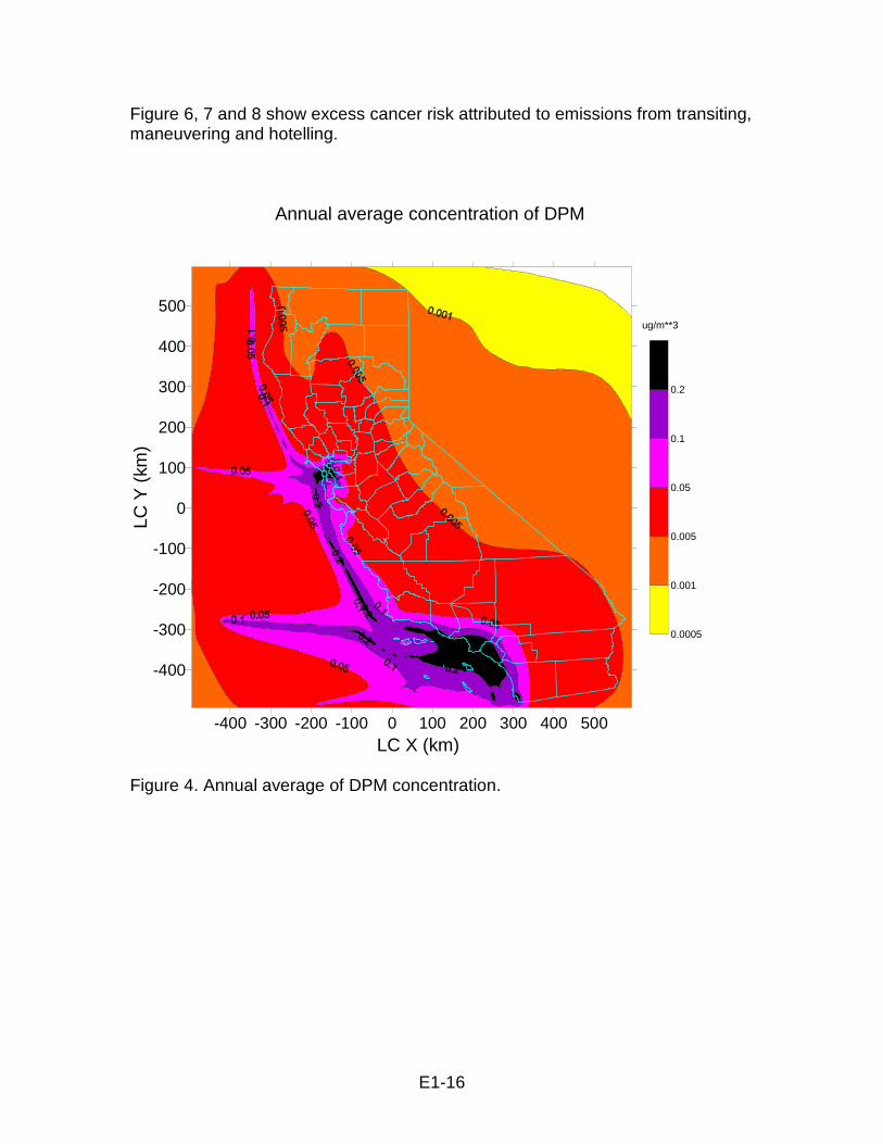
4. Modeling Results CALPUFF was run with the previously described inputs and model setup, including a 2005 OGV emission inventory and 2002 meteorological data. Hourly concentrations of DPM were generated. The results presented illustrate estimated on-shore impact strictly from OGV emissions. Both dry and wet deposition is considered in the modeling. Dry deposition is determined by deposition velocity which is calculated with a resistance deposition model. Wet deposition is determined by a number of factors including precipitation rate and a scavenging coefficient. Figure 4 presents model-estimated spatial concentration isopleths for annual average DPM concentrations. The unit of concentration is µg/m3. The excess cancer risk due to the DPM concentrations that are illustrated in Figure 4 is shown in Figure 5. The risk was calculated using the annual average DPM concentrations predicted by CALPUFF, and an estimated cancer risk of 318 excess cancer cases per million people breathing air with 1 µg/m3 DPM over a lifetime. The excess cancer risk factor is based on the 80th percentile breathing rate. The potential cancer risks were estimated using standard risk assessment procedures based on the annual average concentration of DPM predicted by the model and a health risk factor (referred to as a cancer potency factor) that correlates cancer risk to the amount of DPM inhaled. The methodology used to estimate the potential cancer risks is consistent with the Tier-1 analysis presented in OEHHA’s Air Toxics Hot Spots Program Guidance Manual for Preparation of Health Risk Assessments (OEHHA, 2003). A Tier-1 analysis assumes that an individual is exposed to an annual average concentration of a pollutant continuously for 70 years.1 The cancer potency factor was developed by the OEHHA and approved by the State’s Scientific Review Panel on Toxic Air Contaminants (SRP) as part of the process of identifying diesel PM emission as a toxic air contaminant (TAC). The estimated DPM concentrations and cancer risk levels produced by a risk assessment are based on a number of assumptions. Many of the assumptions are designed to be health protective so that potential risks to individuals are not underestimated. Therefore, the actual cancer risk calculated is intentionally designed to avoid under-prediction. There are also many uncertainties in the health values used in the risk assessment.

1According to the OEHHA Guidelines, the relatively health-protective assumptions incorporated into the Tier-1 risk assessment make it unlikely that the risks are underestimated for the general population.

E1-16

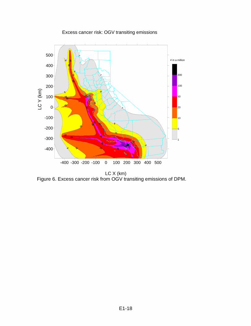
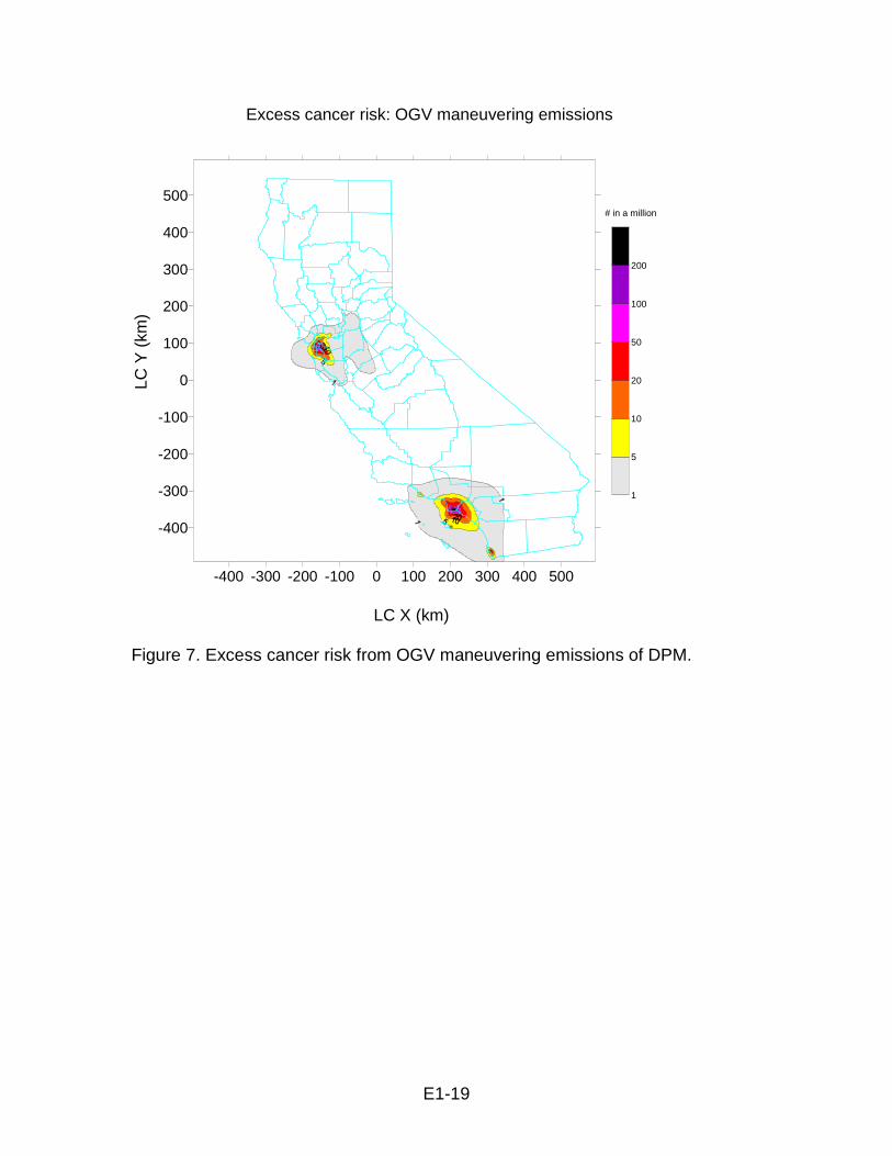
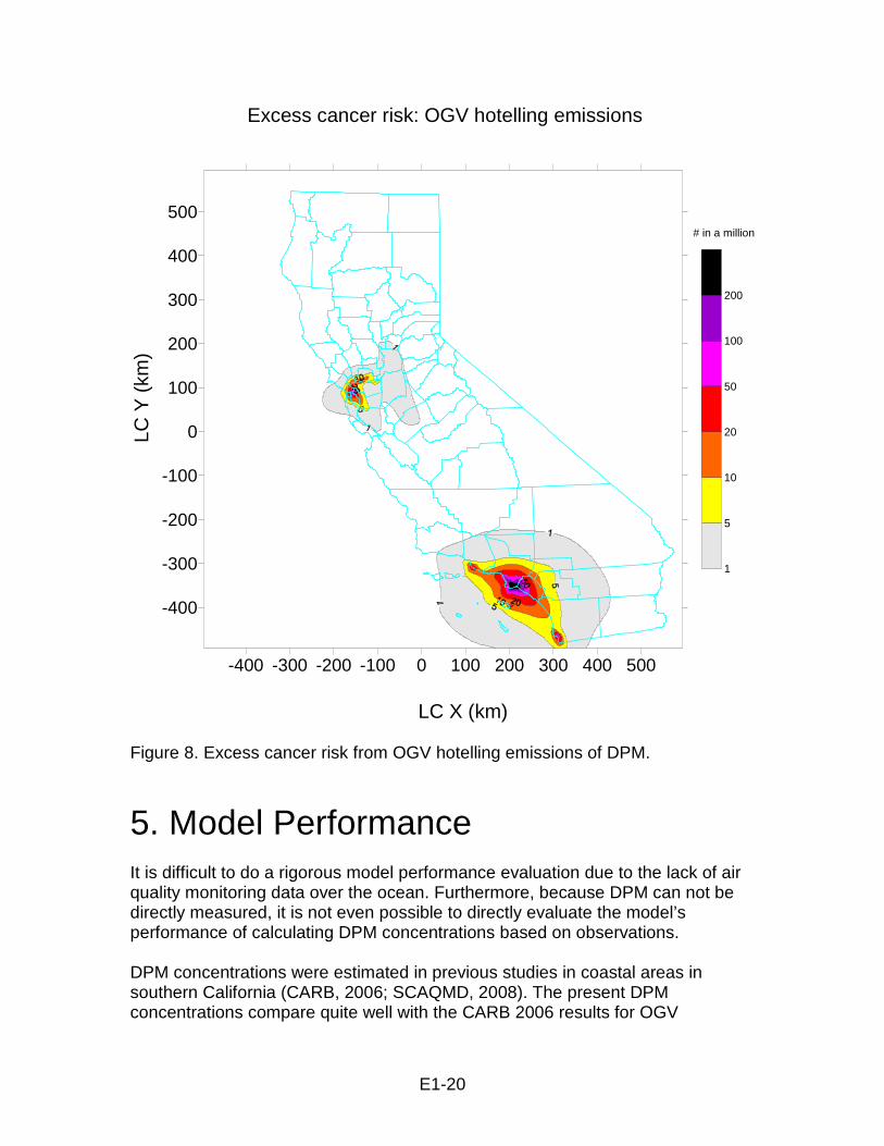
Figure 6, 7 and 8 show excess cancer risk attributed to emissions from transiting, maneuvering and hotelling.

-400 -300 -200 -100 0 100 200 300 400 500

-400

-300

-200

-100

0

100

200

300

400

500

0.0005

0.001

0.005

0.05

0.1

0.2

Annual average concentration of DPM

ug/m**3

LC X (km)

LC Y

(km

)

Figure 4. Annual average of DPM concentration.

E1-17

-400 -300 -200 -100 0 100 200 300 400 500

-400

-300

-200

-100

0

100

200

300

400

500

1

5

10

20

50

100

200

Excess cancer risk: all OGV emissions

# in a million

LC X (km)

LC Y

(km

)

Figure 5. Excess cancer risk from OGV emissions of DPM.

(Transiting, Maneuvering, and Hotelling)

E1-18

-400 -300 -200 -100 0 100 200 300 400 500

-400

-300

-200

-100

0

100

200

300

400

500

1

5

10

20

50

100

200

Excess cancer risk: OGV transiting emissions

# in a million

LC X (km)

LC Y

(km

)

Figure 6. Excess cancer risk from OGV transiting emissions of DPM.

E1-19

-400 -300 -200 -100 0 100 200 300 400 500

-400

-300

-200

-100

0

100

200

300

400

500

1

5

10

20

50

100

200

Excess cancer risk: OGV maneuvering emissions

# in a million

LC X (km)

LC Y

(km

)

Figure 7. Excess cancer risk from OGV maneuvering emissions of DPM.

E1-20

-400 -300 -200 -100 0 100 200 300 400 500

-400

-300

-200

-100

0

100

200

300

400

500

1

5

10

20

50

100

200

Excess cancer risk: OGV hotelling emissions

# in a million

LC X (km)

LC Y

(km

)

Figure 8. Excess cancer risk from OGV hotelling emissions of DPM.

5. Model Performance It is difficult to do a rigorous model performance evaluation due to the lack of air quality monitoring data over the ocean. Furthermore, because DPM can not be directly measured, it is not even possible to directly evaluate the model’s performance of calculating DPM concentrations based on observations. DPM concentrations were estimated in previous studies in coastal areas in southern California (CARB, 2006; SCAQMD, 2008). The present DPM concentrations compare quite well with the CARB 2006 results for OGV

E1-21

emissions. The MATES III study (SCAQMD, 2008) included all emission source categories and the spatial distribution of emissions for each emission categories are quite different (e.g., the distributions of OGV and of diesel trucks). The present modeling results (for OGV emissions only) are quite similar to MATES III results for ship emissions, and the location of highest DPM concentrations is near ports of Los Angeles and Long Beach where the highest OGV emissions occur. Sensitivity tests were conducted to examine the effect of source height and of initial mixing. Three sets of parameters were used: (1) source height at 10 m with 100 m initial mixing; (2) 20 m source height and 20 m initial mixing; and (3) 40 m source height and 10 m initial mixing. Because of the computational burden, the tests were carried out with a subset of emission sources and with January 2002 meteorology. The concentration isopleths looked very similar and the on-shore concentrations were almost identical.

6. Reference (ARB, 2000) Risk Reduction Plan to Reduce Particulate Matter Emissions from Diesel-Fueled Engines and Vehicles, Air Resources Board, September 2000. (ARB, 2006a) State of California, Air Resources Board, Emission Reduction Plan for Ports and Goods Movement in California, April, 2006 (ARB, 2006b) State of California, Air Resources Board, Diesel Particulate Matter Exposure Assessment Study for the Ports of Los Angeles and Long Beach, April 2006 http://www.arb.ca.gov/regact/marine2005/portstudy0406.pdf (ARB, 2008) State of California, Air Resources Board, Diesel Particulate Matter Health Risk Assessment for the West Oakland Community (Draft), Preliminary Summary of Results, March 2008 http://www.arb.ca.gov/ch/communities/ra/westoakland/documents/draftsummary031908.pdf

Scire J.S., D.G. Strimaitis, R.J. Yamartino. “A User's Guide for the CALPUFF Dispersion Model.” Earth Tech, Concord, MA, January 2000. http://www.epa.gov/scram001/dispersion_prefrec.htm#calpuff Scire J.S., F. Robe, F.E.. Fernau, R.J. Yamartino. “A User's Guide for the CALMET Meteorological Model.” Earth Tech, Concord, MA, January 2000. South Coast Air Quality Management District (SCAQMD). “MATES III, Appendix IX – Regional Modeling Analyses”, Diamond Bar, CA, January 2008.