Embed Size (px)
Citation preview

APPENDIX 12-A
Habitat Suitability Modelling
PORT METRO VANCOUVER | Roberts Bank Terminal 2
This page is intentionally left blank
ROBERTS BANK TERMINAL 2
TECHNICAL REPORT
Habitat Suitability Modelling Study
Prepared for: Port Metro Vancouver 100 The Pointe, 999 Canada Place Vancouver, BC V6C 3T4 Prepared by: Hemmera Envirochem Inc. 18
th Floor, 4730 Kingsway
Burnaby, BC V5H 0C6 File: 302-042.02 December 2014

Port Metro Vancouver Hemmera RBT2 – Habitat Suitability Modelling Study December 2014
Technical Report / Technical Data Report Disclaimer
The Canadian Environmental Assessment Agency determined the scope of the proposed Roberts Bank
Terminal 2 Project (RBT2 or the Project) and the scope of the assessment in the Final Environmental
Impact Statement Guidelines (EISG) issued January 7, 2014. The scope of the Project includes the
project components and physical activities to be considered in the environmental assessment. The scope
of the assessment includes the factors to be considered and the scope of those factors. The
Environmental Impact Statement (EIS) has been prepared in accordance with the scope of the Project
and the scope of the assessment specified in the EISG. For each component of the natural or human
environment considered in the EIS, the geographic scope of the assessment depends on the extent of
potential effects.
At the time supporting technical studies were initiated in 2011, with the objective of ensuring adequate
information would be available to inform the environmental assessment of the Project, neither the scope
of the Project nor the scope of the assessment had been determined.
Therefore, the scope of supporting studies may include physical activities that are not included in the
scope of the Project as determined by the Agency. Similarly, the scope of supporting studies may also
include spatial areas that are not expected to be affected by the Project.
This out-of-scope information is included in the Technical Report (TR)/Technical Data Report (TDR) for
each study, but may not be considered in the assessment of potential effects of the Project unless
relevant for understanding the context of those effects or to assessing potential cumulative effects.
Port Metro Vancouver Hemmera RBT2 – Habitat Suitability Modelling Study - i - December 2014
EXECUTIVE SUMMARY
The Roberts Bank Terminal 2 Project (RBT2 or Project) is a proposed new three-berth marine terminal at
Roberts Bank in Delta, B.C. that could provide 2.4 million TEUs (twenty-foot equivalent unit containers) of
additional container capacity annually. The Project is part of Port Metro Vancouver’s Container Capacity
Improvement Program, a long-term strategy to deliver projects to meet anticipated growth in demand for
container capacity to 2030.
Port Metro Vancouver has retained Hemmera to undertake environmental studies related to the Project.
This Technical Report describes the results of the Habitat Suitability Modelling study for orange sea pens
(Ptilosarcus gurneyi), Dungeness crabs (Metacarcinus magister), and Pacific sand lance (Ammodytes
hexapterus).
Habitat suitability models (HSM) are analytical tools that are used to quantify the relationship between the
spatial distribution and/or productivity of a species and environmental variables. Habitat suitability
modelling was used to quantify areas of potentially suitable habitat for orange sea pens (Ptilosarcus
gurneyi), Dungeness crabs (Metacarcinus magister), and Pacific sand lance (Ammodytes hexapterus)
under existing conditions and to predict changes in suitable habitat availability to each species group with
construction of RBT2. Habitat Suitability Indices (HSI) were constructed for Dungeness crab and Pacific
sand lance, which evaluate habitat quality and availability determined from literature or field data. In
contrast, georeferenced species occurrence and environmental data allowed a species distribution model
(SDM) to be constructed for orange sea pens, with spatially explicit predictions of environmental
suitability.
The orange sea pen SDM results indicate that the development of RBT2 will result in loss of 86.1 ha
(27%) of suitable (i.e., high + moderate suitability) habitat, leaving ~232.3 ha of habitat suitable for orange
sea pens at Roberts Bank. A net gain (3.4 ha) in the amount of high suitability habitat is predicted even
before mitigation, since it is predicted that existing moderate suitability habitat will be enhanced in
localised areas around the new Terminal, especially as a result of accelerated water flow and an
associated increase in food delivery to sea pens.
Predictions based on the HSI indicate that substantial amounts of high and moderate suitability
Dungeness crab habitat will remain available to Dungeness crabs outside the Project footprint.
Dungeness juveniles, gravid females, and adults are predicted to lose 9 ha, 57 ha, and 136 ha of high
suitability habitat respectively, representing 0.5%, 11%, and 13% of highly suitable habitat in the study
area. The permanent displacement from high suitability subtidal sand habitat is predicted to have a minor
negative impact on Dungeness crab productivity.

Port Metro Vancouver Hemmera RBT2 – Habitat Suitability Modelling Study - ii - December 2014
Pacific sand lance are predicted to lose 119 ha of moderate suitability and 3.5 ha of high suitability
burying habitat as a result of terminal placement and berth pocket creation, constituting approximately
14% of available suitable subtidal burying habitat in the study area.
Taken together, the predictions from the HSMs enable quantification of changes in habitat, and facilitate
the planning of mitigation measures.
Port Metro Vancouver Hemmera RBT2 – Habitat Suitability Modelling Study - iii - December 2014
TABLE OF CONTENTS
EXECUTIVE SUMMARY ............................................................................................................................... I
1.0 INTRODUCTION .............................................................................................................................. 1
1.1 PROJECT BACKGROUND ........................................................................................................ 1
1.2 HABITAT SUITABILITY MODELLING STUDY OVERVIEW .............................................................. 1
2.0 REVIEW OF EXISTING LITERATURE AND DATA ....................................................................... 2
2.1 HABITAT SUITABILITY MODELLING BACKGROUND .................................................................... 2
2.2 FOCAL SPECIES .................................................................................................................... 3
3.0 METHODS ....................................................................................................................................... 4
3.1 STUDY AREA ......................................................................................................................... 4
3.2 TEMPORAL SCOPE................................................................................................................. 4
3.3 STUDY METHODS .................................................................................................................. 6
3.3.1 Environmental Variables ........................................................................................ 6
3.3.1.1 Sediment Grain Size ............................................................................ 6
3.3.1.2 Bottom Current Velocity ....................................................................... 8
3.3.1.3 Wave Height ...................................................................................... 10
3.3.1.4 Salinity ............................................................................................... 10
3.3.1.5 Water Depth ....................................................................................... 10
3.3.1.6 Slope and Bathymetric Position Index (BPI) ...................................... 10
4.0 ORANGE SEA PEN HSM.............................................................................................................. 12
4.1 REVIEW OF EXISTING LITERATURE AND DATA........................................................................ 12
4.1.1 Distribution ........................................................................................................... 12
4.1.2 Habitat Requirements and Limiting Factors ......................................................... 12
4.2 METHODS FOR DEVELOPMENT OF HSM ............................................................................... 14
4.2.1 Environmental Variable Data from Roberts Bank ................................................ 14
4.2.1.1 Current and Wave Profiling ................................................................ 14
4.2.1.2 Water Column Profiling ...................................................................... 16
4.2.1.3 Sediment Sampling ............................................................................ 16
4.3 RESULTS ............................................................................................................................ 19
4.3.1 Current Profiling ................................................................................................... 19
4.3.2 Wave Profiling ...................................................................................................... 22
4.3.3 Water Column Profiling ........................................................................................ 24

Port Metro Vancouver Hemmera RBT2 – Habitat Suitability Modelling Study - iv - December 2014
4.3.4 Sediment Characteristic ....................................................................................... 26
4.3.5 Species Distribution Model Development ............................................................ 27
4.4 SDM OUTPUTS ................................................................................................................... 28
4.5 DISCUSSION ........................................................................................................................ 29
5.0 DUNGENESS CRAB HSM ............................................................................................................ 34
5.1 REVIEW OF EXISTING LITERATURE AND DATA........................................................................ 34
5.1.1 Distribution ........................................................................................................... 34
5.1.2 Habitat Requirements and Limiting Factors ......................................................... 34
5.1.2.1 Juveniles ............................................................................................ 34
5.1.2.2 Adults ................................................................................................. 35
5.1.2.3 Gravid Females ................................................................................. 35
5.2 METHODS FOR DEVELOPMENT OF HSM ............................................................................... 36
5.3 RESULTS ............................................................................................................................ 38
5.4 DISCUSSION ........................................................................................................................ 41
6.0 PACIFIC SAND LANCE HSM ....................................................................................................... 42
6.1 REVIEW OF EXISTING LITERATURE AND DATA........................................................................ 42
6.1.1 Distribution ........................................................................................................... 42
6.1.2 Habitat Requirements and Limiting Factors ......................................................... 43
6.2 METHODS FOR DEVELOPMENT OF HSM ............................................................................... 46
6.3 RESULTS ............................................................................................................................ 47
6.4 DISCUSSION ........................................................................................................................ 52
7.0 GENERAL DISCUSSION .............................................................................................................. 54
7.1 DISCUSSION OF KEY FINDINGS ............................................................................................. 54
7.2 DATA GAPS AND LIMITATIONS .............................................................................................. 55
8.0 CLOSURE ...................................................................................................................................... 57
9.0 REFERENCES ............................................................................................................................... 58
10.0 STATEMENT OF LIMITATIONS ................................................................................................... 69
Port Metro Vancouver Hemmera RBT2 – Habitat Suitability Modelling Study - v - December 2014
List of Tables
Table 1-1 Habitat Suitability Modelling Study Components and Major Objectives. ............................ 1
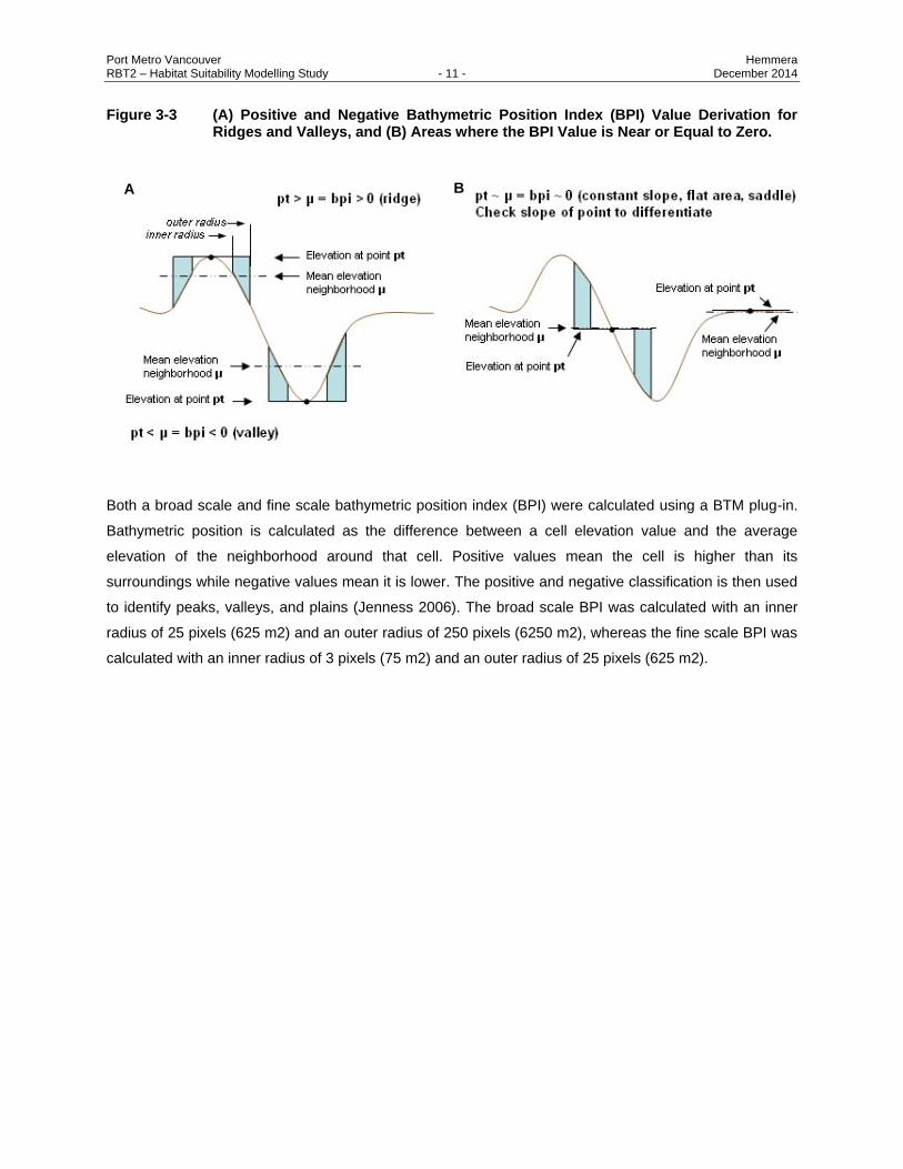
Table 3-1 List of Environmental Factors Input to each Species Habitat Suitability Model (HSM). ..... 6
Table 3-2 Sediment Size Classes with Associated Pacific Sand Lance Suitability Indices. ............... 8
Table 4-1 AWAC and ADCP Instrument Settings for Summer and Winter Deployments. ............... 16
Table 4-2 Comparison of Geometric Mean Sediment Grain Size Composition (%) Among Sites. .. 26
Table 4-3 Habitat Suitability (ha) for Orange Sea Pens (Ptilosarcus gurneyi) in Future Scenarios
With and Without RBT2. ................................................................................................... 29
Table 5-1 Environmental Variable Inputs for Dungeness Crab Weighted Rating Habitat Suitability
Model (HSM). .................................................................................................................... 37
Table 5-2 HSM Outputs Quantifying Areal extent (in ha) of High, Moderate, and Low Habitat
Suitability Dungeness Crab Habitat, by Life Stage, under the Existing and with Project
Scenarios. ......................................................................................................................... 39
Table 5-3 Predicted Losses of High, Moderate, and Low Suitability Habitat With RBT2 (from Table
5.2) and Areas of Overlap (ha) with Project Component Footprints, by Life Stage. ......... 39
Table 6-1 Environmental Variables and Weightings Used in Pacific Sand Lance (PSL) Burying
Habitat Suitability Model (HSM) for Roberts Bank. ........................................................... 47
Table 6-2 Areas (ha) of High, Moderate, and Low Suitability Subtidal Burying Habitat for Pacific
Sand Lance (Ammodytes hexapterus) Without and With RBT2. Habitat Losses are Based
on Direct Footprint Losses, and Do Not Include Indirect Effects from Changes in Coastal
Geomorphology. ................................................................................................................ 49
Table 6-3 Area Lost (ha) of High, Moderate, and Low Suitability Subtidal Burying Habitat for Pacific
Sand Lance (Ammodytes hexapterus), Without and With RBT2, by Project Footprint Area
(Terminal, Dredge Basin, Tug Basin, and Intermediate Transfer Pit (ITP)). Habitat Losses
are Based on Direct Footprint Losses and Do Not Include Indirect Effects from Changes
to Coastal Geomorphology. .............................................................................................. 50
List of Figures (within text)
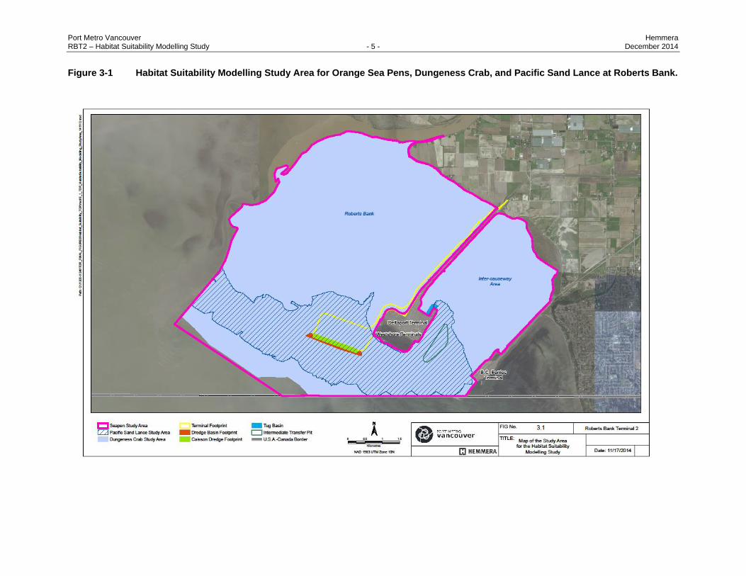
Figure 3-1 Habitat Suitability Modelling Study Area for Orange Sea Pens, Dungeness Crab, and
Pacific Sand Lance at Roberts Bank. ................................................................................. 5
Figure 3-2 IDW Interpolation of Geometric Mean Sediment Grain Size at Roberts Bank. .................. 9
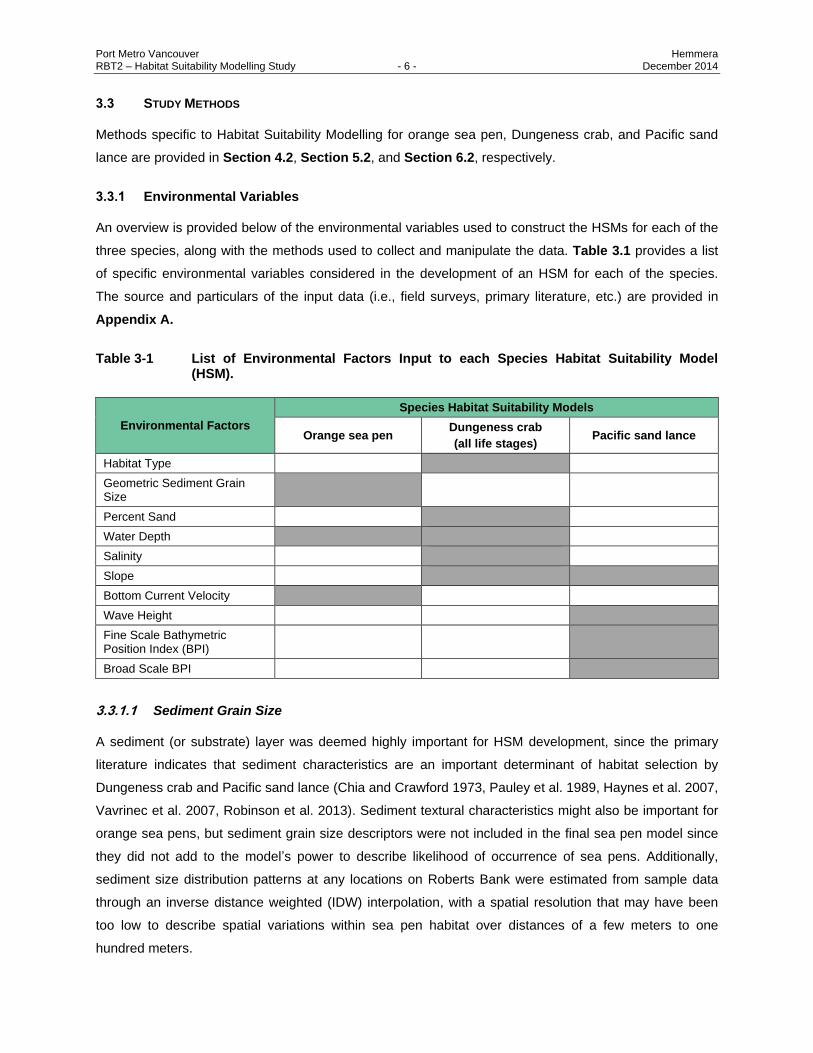
Figure 3-3 (A) Positive and Negative Bathymetric Position Index (BPI) Value Derivation for Ridges
and Valleys, and (B) Areas where the BPI Value is Near or Equal to Zero. ..................... 11
Figure 4-1 Placement of Current Profiling Equipment in Areas of Continuous to Dense (ADCP) and
Few to Patchy (AWAC) Orange Sea Pens. ...................................................................... 15
Port Metro Vancouver Hemmera RBT2 – Habitat Suitability Modelling Study - vi - December 2014
Figure 4-2 Locations of Conductivity, Temperature and Depth (CTD) Profiles at Roberts Bank. ...... 17
Figure 4-3 Sediment Sampling Locations at Roberts Bank used in Orange Sea Pen Statistical
Analyses ............................................................................................................................ 18
Figure 4-4 Example of AWAC and ADCP Near-Bed Currents (Magnitude and Direction) for a Large
Tide Period from January 7th to January 11th, 2013. ....................................................... 19
Figure 4-5 ADCP Profiles over the First Five Bins (up to 4.11 m above the bed) for One Tide Cycle
(January 11th-12th). Note that a zero velocity was assumed for the bed. ....................... 21
Figure 4-6 AWAC Profiles over the First Three Bins (up to 3.9 m above the bed) for One Tide Cycle
(January 11th-12th). Note that a zero velocity was assumed for the bed. ....................... 21
Figure 4-7 Average Velocity at 2.4 m Above the Bed During Rising Tide and Ebbing Tide for AWAC
and ADCP for the Full Period of Record. .......................................................................... 22
Figure 4-8 Characteristic Wave Heights at Patchy (AWAC) and dense (ADCP) Orange Sea Pen
Sites over the Full Period of Record. ................................................................................ 23
Figure 4-9 Wave Heights, Tide Levels and Near-Bed Current Velocities at Patchy (AWAC) and
Dense (ADCP) Orange Sea Pen Sites During a Large Storm Event on December 19th,
2012 and Subsequent Days. ............................................................................................. 23
Figure 4-10 Percent Sediment (Sand, Clay, Silt and Gravel) Associated with Areas of Dense,
Patchily-Distributed (‘Patchy’), and No Orange Sea Pens................................................ 26
Figure 4-11 Habitat Suitability for Orange Sea Pens at Roberts Bank, as Identified by the Species
Distribution Model, A) Without RBT2 (Existing Conditions), and B) With RBT2. .............. 31
Figure 5-1 Existing Habitat Suitability for Dungeness Crabs at Roberts Bank, by Life Stage, as
Identified by the Habitat Suitability Model (HSM). ............................................................ 40
Figure 6-1 Habitat Suitability of Pacific sand lance at Roberts Bank, as Identified by the Habitat
Suitability Model (HSM), A) Without RBT2 (Existing Conditions), and B) With RBT2. Input
Environmental Variables were Sediment Grain Size, Bottom Current Velocity, and Water
Depth. ................................................................................................................................ 51
List of Appendices
Appendix A Data Origins of Environmental Variables.
Appendix B Geospatial Interpolations – Inverse Distance Weighting (IDW).
Appendix C Habitat Layer Maps for the Dungeness Crab Life Stages and Pacific Sand Lance HSMs.
Appendix D Table of SDM Parameter Outputs for the Sea Pen, Coefficient Estimate, Standard Error,
z-score, and p value.
Port Metro Vancouver Hemmera RBT2 – Habitat Suitability Modelling Study - 1 - December 2014
1.0 INTRODUCTION
1.1 PROJECT BACKGROUND
The Roberts Bank Terminal 2 Project (RBT2 or Project) is a proposed new three-berth marine terminal at
Roberts Bank in Delta, B.C. that could provide 2.4 million TEUs (twenty-foot equivalent unit containers) of
additional container capacity annually. The Project is part of Port Metro Vancouver’s Container Capacity
Improvement Program, a long-term strategy to deliver projects to meet anticipated growth in demand for
container capacity to 2030.
Port Metro Vancouver has retained Hemmera to undertake environmental studies related to the Project.
This Technical Report describes the results of the Habitat Suitability Modelling study for orange sea pens
(Ptilosarcus gurneyi), Dungeness crabs (Metacarcinus magister), and Pacific sand lance (Ammodytes
hexapterus).
1.2 HABITAT SUITABILITY MODELLING STUDY OVERVIEW
A review of existing information and the current state of knowledge was completed for the Habitat
Suitability Modelling Study to identify key data gaps and areas of uncertainty within the general RBT2
area. This Technical Report describes the study findings for key components identified from this gap
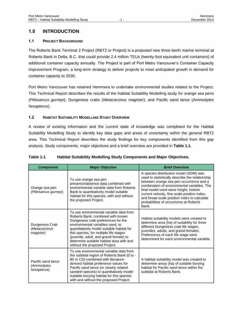
analysis. Study components, major objectives and a brief overview are provided in Table 1.1.
Table 1-1 Habitat Suitability Modelling Study Components and Major Objectives.
Component Major Objective Brief Overview
Orange sea pen (Ptilosarcus gurneyi)
To use orange sea pen presence/absence data combined with environmental variable data from Roberts Bank to quantitatively model suitable habitat for this species, with and without the proposed Project.
A species distribution model (SDM) was used to statistically describe the relationship between orange sea pen occurrence and a combination of environmental variables. The final model used wave height, bottom current velocity, fine scale position index, and broad scale position index to calculate probabilities of occurrence at Roberts Bank.
Dungeness Crab (Metacarcinus magister)
To use environmental variable data from Roberts Bank, combined with known Dungeness crab preferences for the environmental variables used, to quantitatively model suitable habitat for this species, for multiple life stages (juvenile, adult, and gravid female) to determine suitable habitat area with and without the proposed Project.
Habitat suitability models were created to determine area (ha) of suitability for three different Dungeness crab life stages, juveniles, adults, and gravid females. Preferences of each life stage were determined for each environmental variable.
Pacific sand lance (Ammodytes hexapterus)
To use environmental variable data from the subtidal region of Roberts Bank (0 to -80 m CD) combined with literature-derived habitat preference values for Pacific sand lance (or closely related sandeel species) to quantitatively model suitable burying habitat for this species with and without the proposed Project.
A habitat suitability model was created to determine areas (ha) of suitable burying habitat for Pacific sand lance within the subtidal at Roberts Bank.

Port Metro Vancouver Hemmera RBT2 – Habitat Suitability Modelling Study - 2 - December 2014
2.0 REVIEW OF EXISTING LITERATURE AND DATA
2.1 HABITAT SUITABILITY MODELLING BACKGROUND
Habitat suitability models (HSM) are analytical tools that are used to quantify the relationship between the
spatial distribution and/or productivity of a species and environmental variables. HSMs allow biologists to
make model-based predictions about potential species distributions based on the availability of resources
or suitable habitats within an area under study (Aarts et al. 2013). Environmental variables are defined as
abiotic or biotic components of the environment that are important for the growth and survival of
individuals or populations of a species (Ahmadi-Nedushan et al. 2006). Examples of measurable
variables that may contribute to species habitat preferences include vegetation cover, substrate type,
water depth, current velocity, and the availability of refuge or breeding sites (Hirzel and Le Lay 2008). To
the extent that chosen variables are causally connected to or correlated with a species` occurrence or
productivity across the sampled sites, HSMs can be used to make inferences about the ecological
requirements of a species and predictions about its potential distribution outside of a sampled area -
although such predictions include some level of uncertainty (Hirzel and Le Lay 2008, Cianfrani et al.
2010, Latif et al. 2013). The integration of GIS software advancements (Hirzel and Guisan 2002,
Rotenberry et al. 2006) and spatial modeling tools such as marine geospatial ecology tools (MGET) and
broad-scale, high-resolution terrain mapping techniques enable us to measure a species’ association with
quantifiable landscape features.
Habitat Suitability Models cover a range of model types, including Habitat Suitability Indices (HSIs) and
Species Distribution Models (SDMs). HSIs are designed to represent the relative preference of target
species for an independent or composite set of chosen habitat variables (Ahmadi-Nedushan et al. 2006).
Common approaches for quantifying HSIs include combining observations from the field with existing
knowledge about a species’ preferred habitat attributes (Ahmadi-Nedushan et al. 2006). This is generally
achieved through the calculation of statistical relationships between species observations and
environmental descriptors, though approaches that include mechanistic modelling and expert opinion also
exist (Guisan et al. 2013). If empirical data are not available for a study area, data from previous studies
as documented in the scientific literature and professional judgement can be used (Ahmadi-Nedushan et
al. 2006). HSIs may also include qualitative categories of habitat suitability that reflect a species’
preference for a habitat, such as low, moderate, or high suitability (Ahmadi-Nedushan et al. 2006).
Additionally, HSIs can be calculated for specific life stages of a target species, such as juvenile, spawning
adult or larval life stages in fish or marine invertebrates (Minns et al. 2011).
Habitat suitability models, such as HSIs, evaluate habitat quality and availability that may not be location
specific. When georeferenced species-occurrence and environmental distribution data are available,
species distribution models (SDMs) can be used to calculate spatially explicit predictions of environmental
suitability for species. Species distribution models use statistical tools such as generalised linear models

Port Metro Vancouver Hemmera RBT2 – Habitat Suitability Modelling Study - 3 - December 2014
(GLMs) to create statistical relationships among species occurrence and environmental predictor
variables. The GLMs use species occurrence as a function of environmental variables (e.g., salinity,
slope, current velocity) to produce likelihood estimates of species occurrence in areas without
observational presence/absence data (Rotenberry et al. 2006). Validation of these models can be
achieved using a portion of the data not used for model creation to provide an estimate of model strength.
The use of HSMs is frequently applied to the management of marine populations based on an adequate
understanding of how environmental variables influence species productivity (Hirzel and Le Lay 2008,
Cianfrani et al. 2010, Minns et al. 2011). Information on where species are located in the marine
environment can be used to define key habitats, or to predict the effects of habitat loss on species
distributions (Hirzel and Le Lay 2008, Minns et al. 2011). Model-based predictions can also be used to
inform adaptive management strategies and mitigation actions that require either identifying reintroduction
sites or creating new suitable habitats to compensate for losses associated with anthropogenic
development or climate change (Hirzel and Le Lay 2008, Cianfrani et al. 2010).
2.2 FOCAL SPECIES
Three species were selected for habitat suitability modelling; orange sea pens (Ptilosarcus gurneyi),
selected for their role in providing biogenic habitat for a number of fish and invertebrate species;
Dungeness crabs (Metacarcinus magister), selected for their importance in commercial, recreational, and
Aboriginal (CRA) fisheries; and Pacific sand lance (Ammodytes hexapterus), selected due to their
reliance on subtidal habitat and their importance to higher trophic level organisms, including other marine
fish species, coastal birds, and marine mammals. Detailed literature reviews for orange sea pen,
Dungeness crab, and Pacific sand lance are provided in Section 4.1, Section 5.1, and Section 6.1,
respectively.
Port Metro Vancouver Hemmera RBT2 – Habitat Suitability Modelling Study - 4 - December 2014
3.0 METHODS
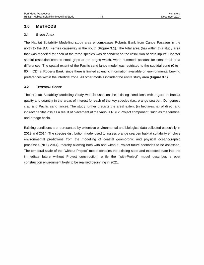
3.1 STUDY AREA
The Habitat Suitability Modelling study area encompasses Roberts Bank from Canoe Passage in the
north to the B.C. Ferries causeway in the south (Figure 3.1). The total area (ha) within this study area
that was modeled for each of the three species was dependent on the resolution of data inputs: Coarser
spatial resolution creates small gaps at the edges which, when summed, account for small total area
differences. The spatial extent of the Pacific sand lance model was restricted to the subtidal zone (0 to -
80 m CD) at Roberts Bank, since there is limited scientific information available on environmental burying
preferences within the intertidal zone. All other models included the entire study area (Figure 3.1).
3.2 TEMPORAL SCOPE
The Habitat Suitability Modelling Study was focused on the existing conditions with regard to habitat
quality and quantity in the areas of interest for each of the key species (i.e., orange sea pen, Dungeness
crab and Pacific sand lance). The study further predicts the areal extent (in hectares:ha) of direct and
indirect habitat loss as a result of placement of the various RBT2 Project component, such as the terminal
and dredge basin.
Existing conditions are represented by extensive environmental and biological data collected especially in
2013 and 2014. The species distribution model used to assess orange sea pen habitat suitability employs
environmental predictions from the modelling of coastal geomorphic and physical oceanographic
processes (NHC 2014), thereby allowing both with and without Project future scenarios to be assessed.
The temporal scale of the “without Project” model contains the existing state and expected state into the
immediate future without Project construction, while the “with-Project” model describes a post
construction environment likely to be realised beginning in 2021.
Port Metro Vancouver Hemmera RBT2 – Habitat Suitability Modelling Study - 5 - December 2014
Figure 3-1 Habitat Suitability Modelling Study Area for Orange Sea Pens, Dungeness Crab, and Pacific Sand Lance at Roberts Bank.
Port Metro Vancouver Hemmera RBT2 – Habitat Suitability Modelling Study - 6 - December 2014
3.3 STUDY METHODS
Methods specific to Habitat Suitability Modelling for orange sea pen, Dungeness crab, and Pacific sand
lance are provided in Section 4.2, Section 5.2, and Section 6.2, respectively.
3.3.1 Environmental Variables
An overview is provided below of the environmental variables used to construct the HSMs for each of the
three species, along with the methods used to collect and manipulate the data. Table 3.1 provides a list
of specific environmental variables considered in the development of an HSM for each of the species.
The source and particulars of the input data (i.e., field surveys, primary literature, etc.) are provided in
Appendix A.
Table 3-1 List of Environmental Factors Input to each Species Habitat Suitability Model (HSM).
Environmental Factors
Species Habitat Suitability Models
Orange sea pen Dungeness crab
(all life stages) Pacific sand lance
Habitat Type
Geometric Sediment Grain Size
Percent Sand
Water Depth
Salinity
Slope
Bottom Current Velocity
Wave Height
Fine Scale Bathymetric Position Index (BPI)
Broad Scale BPI
3.3.1.1 Sediment Grain Size
A sediment (or substrate) layer was deemed highly important for HSM development, since the primary
literature indicates that sediment characteristics are an important determinant of habitat selection by
Dungeness crab and Pacific sand lance (Chia and Crawford 1973, Pauley et al. 1989, Haynes et al. 2007,
Vavrinec et al. 2007, Robinson et al. 2013). Sediment textural characteristics might also be important for
orange sea pens, but sediment grain size descriptors were not included in the final sea pen model since
they did not add to the model’s power to describe likelihood of occurrence of sea pens. Additionally,
sediment size distribution patterns at any locations on Roberts Bank were estimated from sample data
through an inverse distance weighted (IDW) interpolation, with a spatial resolution that may have been
too low to describe spatial variations within sea pen habitat over distances of a few meters to one
hundred meters.

Port Metro Vancouver Hemmera RBT2 – Habitat Suitability Modelling Study - 7 - December 2014
To create the substrate layers for the Dungeness crab and Pacific sand lance HSMs, empirical data from
Roberts Bank were used (Hemmera 2014a). Extensive surface sediment sampling (top ~ 2 cm) was
conducted in both intertidal and subtidal areas using a 0.1 m2 Van Veen grab between April 2012 and
July 2013.
The calculated geometric mean sediment grain size was used as the primary descriptor of spatially
variable sediment characteristics for the Pacific sand lance HSM, while percent sand was used for
the Dungeness crab HSM. The geometric mean grain size was used for Pacific sand lance since
literature-based sediment preference values are more often reported as sediment classes (classification
as gravel, sand, silt or clay) than fractional percentages (Pinto et al. 1984, Haynes et al. 2007, Robinson
et al. 2013).
For the Pacific sand lance HSM, geometric mean grain size for each sediment sample from Roberts Bank
was determined from percentile values obtained from linear interpolation between log-transformed grain
size values in millimeters (mm) (Bunte and Abt 2001). The nth root geometric approach was used to
compute mean grain size, based on the percentiles at the point of curvature (Bunte and Abt 2001):
Mean sediment grain size (mm) = √𝐷16 + 𝐷84
There were fewer sediment sample locations in the subtidal zone than intertidal zone (Hemmera 2014a);
therefore, creation of the geometric mean sediment grain size layer using IDW interpolation resulted in
gaps (i.e., ~55 ha or 3% of the ~1,432 ha Pacific sand lance study area). Results for the sand lance
model are thus presented as percent losses of both the study area (0 to -80m CD) and the modelled area
(see Section 6.3 Pacific sand lance Results).
In contrast, Dungeness crab habitat preferences are often reported using general class terminology
(i.e., preference for sand) (Dethier 2006, Vavrinec et al. 2007). Accordingly, percent composition was
used to calculate the amount of sand in each grab sample, based on proportion of each sample between
63 µm and 2 mm in diameter, for use in the Dungeness crab HSM.
Geometric mean sediment grain size and percent sand classified seabed maps were created using
inverse distance weighted interpolation (IDW). A uniform grid size of 20 m was applied, along with a
variable search radius of 500 m and a maximum of 12 sample points. For more details on IDW
calculations, please refer to Appendix C. Figure 3.2 shows IDWs of A) geometric mean sediment grain
size, and B) percent sand distribution at Roberts Bank.
Sediment maps were used to identify areas of varying sediment suitability for each of the three species of
interest. For Pacific sand lance, specific class breaks for mean sediment grain size were chosen based
on literature values (Table 3.2). For Dungeness crab, a scaled preference for increasing percent sand

Port Metro Vancouver Hemmera RBT2 – Habitat Suitability Modelling Study - 8 - December 2014
composition was determined using information from literature, field data, and professional judgement. A
percent sand sediment map was used in the orange sea pen SDM, but was excluded from the variables
used in the final model since it did not improve the ability of the model to describe sea pen presence
or absence.
Table 3-2 Sediment Size Classes with Associated Pacific Sand Lance Suitability Indices.
Geometric Mean Sediment Size (mm) Adult Suitability Index (SI)
0 - 0.125 1
0.125 - 0.25 2
0.25 - 2.0 3
2.0 + 1
3.3.1.2 Bottom Current Velocity
Bottom current velocity was modeled for Roberts Bank as part of a coastal geomorphology study of the
area (NHC 2014). Published bottom current preferences for Pacific sand lance indicate an optimal range
of 25 – 63 cm/s (Robinson et al. 2013), as moderate to high currents are thought to remove silt and result
in higher oxygenated sediments (Robards et al. 1999). To represent bottom current velocity (cm/s) values
relevant to Pacific sand lance, both 90th and 50
th percentile model outputs from the NHC geomorphic
model were used. 90th percentile data were deemed reasonable to define the upper limit of the preference
range (i.e., 63 cm/s) as they are only infrequently exceeded (i.e., 10% of the time) (Derek Ray, pers.
comm. 2014). 50th percentile values were considered reasonable to define the lower bound (i.e., 25 cm/s)
as areas below this are generally low velocity zones (D. Ray, pers. comm). Surface layers were
generated for each dataset and merged in Arc GIS 10.2© to obtain a final bottom current surface layer
identifying areas with bottom current velocity values ≥25 cm/s 50% of the time and ≤63 cm/s 90% of
the time.

Port Metro Vancouver Hemmera RBT2 – Habitat Suitability Modelling Study - 9 - December 2014
Figure 3-2 IDW Interpolation of Geometric Mean Sediment Grain Size at Roberts Bank.

Port Metro Vancouver Hemmera RBT2 – Habitat Suitability Modelling Study - 10 - December 2014
3.3.1.3 Wave Height
Wave height was modeled for Roberts Bank as part of a coastal geomorphology study of the area (NHC
2014). Orange sea pen distribution is likely influenced by large wave heights at least at water depths
shallow enough for wind-generated waves to interact with the substrate. The wave base, i.e. maximum
depth at which the passage of a water wave causes significant motion, occurs at a depth equivalent to
half the wave length. The relationship between wave height and wave length is complex; however, both
tend to increase with wind speed and fetch. To best represent the upper threshold of wave heights in the
orange sea pen HSM, 90th percentile model outputs were used, which represent rarer, large wave
events.
3.3.1.4 Salinity
Salinity was modeled for Roberts Bank as part of a coastal geomorphology study of the area (NHC 2014).
50th percentile salinity data were used in the Dungeness crab HSMs, as these mid-range values best
describe the average conditions experienced across the entire Roberts Bank area.
3.3.1.5 Water Depth
A bathymetric digital elevation model (DEM) with a 5 m2 resolution was created by amalgamating
multibeam and LIDAR data from Roberts Bank. Multibeam data were obtained from the Canadian
Hydrographic Service (CHS) via the Geological Survey of Canada (GSC Pacific). Several CHS surveys
from different years (2000, 2001, 2003, 2005, 2008, 2010, and 2011) covering the general area of the
Fraser Delta were available. A comprehensive mosaic of merged bathymetry from all years was provided
by the GSC. High resolution LIDAR used for the DEM was collected for the intertidal region of Roberts
Bank during 2011 surveys.
3.3.1.6 Slope and Bathymetric Position Index (BPI)
The bathymetric surface layer was used to create derived surfaces to be used in the habitat models.
Slope was created using the bathymetric terrain modeler (BTM) plugin for ArcGIS (Wright et al. 2012).
Angle of slope is calculated as the maximum change in elevation over the distance between the cell of
the raster and its eight neighbors. The slope measure identifies the steepest downhill descent from the
cell and produces a map of angular difference at the site.
Port Metro Vancouver Hemmera RBT2 – Habitat Suitability Modelling Study - 11 - December 2014
Figure 3-3 (A) Positive and Negative Bathymetric Position Index (BPI) Value Derivation for Ridges and Valleys, and (B) Areas where the BPI Value is Near or Equal to Zero.
Both a broad scale and fine scale bathymetric position index (BPI) were calculated using a BTM plug-in.
Bathymetric position is calculated as the difference between a cell elevation value and the average
elevation of the neighborhood around that cell. Positive values mean the cell is higher than its
surroundings while negative values mean it is lower. The positive and negative classification is then used
to identify peaks, valleys, and plains (Jenness 2006). The broad scale BPI was calculated with an inner
radius of 25 pixels (625 m2) and an outer radius of 250 pixels (6250 m2), whereas the fine scale BPI was
calculated with an inner radius of 3 pixels (75 m2) and an outer radius of 25 pixels (625 m2).
A B
Port Metro Vancouver Hemmera RBT2 – Habitat Suitability Modelling Study - 12 - December 2014
4.0 ORANGE SEA PEN HSM
4.1 REVIEW OF EXISTING LITERATURE AND DATA
4.1.1 Distribution
Orange sea pens (Ptilosarcus gurneyi) are widely distributed along the Pacific coast of North America
from southern California to Alaska, and are common in low intertidal and shallow subtidal habitats
(Birkeland 1974, Gotshall and Laurent 1979, Shimek 2011). Although most abundant in shallow waters at
depths of -10 to -25 m, they have been observed as deep as -100 m (Birkeland 1974, Shimek 2011).
4.1.2 Habitat Requirements and Limiting Factors
Sea pens are colonial, sessile animals that live anchored in soft sandy bottom sediments (Gotshall and
Laurent 1979). Sea pens commonly form dense aggregations, known as sea pen beds, which can extend
across the seafloor for dozens of kilometers (Tissot et al. 2006, Shimek 2011). At Roberts Bank, sea pen
beds have been consistently observed within mixed sand-silt and diatom covered bottom substrates, but
are largely absent from finer clay and diatom patches (Triton 2004, Archipelago 2009, Hemmera and
Archipelago 2014). Generally, orange sea pens are common along sloped substrates (18⁰ to 25⁰) within
habitats that are subject to strong tidal outflows and oceanic currents (Burd et al. 2008b, Shimek 2011).
Orange sea pens are passive suspension feeders that use specialised feeding polyps to filter zooplankton
(and to a lesser extent phytoplankton) and other organic particles out of the water column (Best 1988,
Shimek 2011). Therefore, sea pens rely on the speed and pattern of ambient water flow for feeding
efficiency, and access to food is optimal when water flow passing through the body of the sea pen is
maximised without causing it to be physically deformed or uprooted by the current (Best 1988).
Unlike other octocorals, sea pens are capable of some locomotion by inflating their bodies with water,
climbing out of the sediment and turning into the currents, allowing them to drift above the seafloor and
relocate (Fuller et al. 2008, Shimek 2011). While adult sea pens are able to withdraw their bodies into the
sediment completely, developing juveniles are more limited in their ability to burrow (Birkeland 1974).
Because individual colonies expand to feed and contract into the sediment at irregular intervals, it is not
clear which environmental factors, such as current velocity, water turbidity, light intensity or food
availability, govern contraction-expansion behaviour (Birkeland 1974, Shimek 2011). Although the
ecological significance of this behaviour is uncertain, it is perceived that burrowing may allow orange sea
pens to be less obvious to predators (Birkeland 1974, Weightman and Arsenault 2002).
Male and female orange sea pens broadcast spawn, releasing large numbers of sperm or eggs into the
water column, where fertilisation occurs externally (Chia and Crawford 1973, Edwards and Moore 2008).
Planktonic larvae are non-feeding, and remain in the plankton for about one week (Shimek 2011). Larval
dispersal and mortality is largely governed by oceanic conditions (Chia and Crawford 1973, Shimek
2011). Once ready to settle, larvae move towards the bottom sediments to search for suitable substrate
Port Metro Vancouver Hemmera RBT2 – Habitat Suitability Modelling Study - 13 - December 2014
(Chia and Crawford 1973). The location where larvae choose to settle appears to be largely governed by
sediment size (0.25 to 0.55 µm diameter) (Shimek 2011) and the presence of other sea pens
(i.e., sediment covered with adult orange sea pen secretions) (Chia and Crawford 1973). Laboratory
studies suggest that if suitable sandy substrate is not available, larvae can delay metamorphosis for up to
~30 days (Chia and Crawford 1973). Larvae that settle on suitable substrate will metamorphose into the
initial polyp, which anchors to the sand and grows rapidly to form the central calcareous stalk of the
animal (Chia and Crawford 1973, Shimek 2011). Once secondary polyps develop, feeding activity begins
(Chia and Crawford 1973, Shimek 2011).
Although orange sea pens are commonly found in dense aggregations, individual sea pens are also
observed within discrete sandy patches (Shimek 2011). Studies by Birkeland (1968, 1974) suggest that
patterns of larval recruitment within Puget Sound are highly dynamic in space and time, and are likely
dependent on the availability of suitable substrate (Chia and Crawford 1973). Such large year-to-year
variability in recruitment is likely to give rise to discontinuities in age and size classes within and between
populations (Birkeland 1974). In Puget Sound, orange sea pen densities have been reported to be as
high as 129 sea pens/m2, with an average density of ~23 sea pens/m
2 (Birkeland 1974). In a more recent
study of Puget Sound, Kyte (2001) suggests that the large populations described by Birkeland (1969) are
no longer present and remaining populations are relatively sparse and patchy. However, orange sea pen
abundance is difficult to estimate as adults are capable of retracting entirely into the sediment, thus many
colonies may be unaccounted for (Birkeland 1974).
Within the Roberts Bank study area, a large aggregation of orange sea pens has been consistently
observed in the area of the Deltaport Terminal delta upper foreslope between depths of -2.5 to -18 m
(west of the Westshore Terminals, Figure 3.1) (Gartner Lee 1992, Triton 2004, Archipelago 2009).
Subsequent towed underwater video and dive surveys in 2011 corroborated previously documented
observations of orange sea pen beds and identified a second dense aggregation at a depth of -3 to -19 m
CD at the southern edge of the Westshore Terminals (Figure 3.1; Hemmera 2014). Orange sea
pens were also found within the Inter-causeway Area and within the tug basin in a few discrete patches
(Figure 3.1; Hemmera 2014). Moreover, the 2011 survey documented the presence of multiple size
(and age) classes including juveniles (<15cm height), indicating that these aggregations may represent a
breeding population or, at least, offer conditions favourable for larval settlement (Hemmera and
Archipelago 2014). Taken together, estimated orange sea pen densities averaged 0.2 and 5.7 sea
pens/m2 within the few to patchy and continuous to dense sections of the aggregation area, respectively
(Hemmera and Archipelago 2014).
Port Metro Vancouver Hemmera RBT2 – Habitat Suitability Modelling Study - 14 - December 2014
4.2 METHODS FOR DEVELOPMENT OF HSM
4.2.1 Environmental Variable Data from Roberts Bank
As little is known about orange sea pen ecology at Roberts Bank, extensive sampling was undertaken to
collect environmental variable data to inform the HSM. Specifically, current and wave profiling, water
column profiling, and sediment sampling were conducted over a two year period from 2011-2013.
4.2.1.1 Current and Wave Profiling
Current and wave profiling were conducted to characterise and compare current profile, directional waves
and bottom temperature between sites of high and low orange sea pen density, and to investigate any
perceptible differences. Current velocity and directional wave profiles were collected at two locations at
Roberts Bank using a 600 kHz Teledyne RDI Acoustic Doppler Current Profiler (ADCP) and a 1,000 kHz
Nortek Acoustic Wave and Current Profiler (AWAC). The instruments were deployed for two discrete
periods by a SCUBA team from Foreshore Technologies: first for a one month period in the summer
(August 8 - September 9, 2012) and, second, for a two month period in the winter (December 17, 2012 -
February 20, 2013). The ADCP was installed in a dense area of orange sea pens while the AWAC was
placed in an adjacent area where orange sea pens were sparse or absent (Figure 4.1). Both instruments
were attached to bottom frames and sat at a similar contour elevation at approximately -4m deep.
Currents were recorded every 10 minutes and waves every hour. Small differences were detected
between instruments, but the settings were similar enough to allow for comparison of results at each site.
The instruments output similar wave statistics (significant wave height, mean 1/10 wave height, maximum
and mean wave height, peak and mean wave period, peak and mean wave direction) and 3D-velocities in
the water column, which can be converted into current amplitude and direction for each bin. Table 4.1
depicts the deployment settings for each device. Instrument stability was confirmed by reviewing pitch
and roll data (measures of rotation) to ensure that neither instrument had moved and that the resulting
data was reliable.
Quality assurance/quality control (QA/QC) checks on the data were completed by ASL Environmental
Services (ASL), who reported that full data sets were collected by all instruments with excellent quality.
The resulting raw data were further analysed by Northwest Hydraulics Consultants (NHC).
Near-bed current velocities are of primary interest when assessing orange sea pen habitat, as individuals
are typically 0.30 m to 0.40 m tall (Archipelago 2011). However, there is a limitation in interpreting the
near-bed velocities that may be preferred by sea pens based on data from the instruments, due to the
presence of a blanking distance immediately above each instrument for which current is not measured
directly. The blanking distance for the AWAC is 0.9 m and the ADCP is 1.61 m. To correct for the
difference in blanking distances during analysis, the second bin of the AWAC (centered at 2.4 m above
bed) and the second bin of ADCP (centered at 2.36 m above bed) were compared. Paired t-tests were
performed on the two datasets using the statistical software SYSTAT to analyse the differences.

Port Metro Vancouver Hemmera RBT2 – Habitat Suitability Modelling Study - 15 - December 2014
Figure 4-1 Placement of Current Profiling Equipment in Areas of Continuous to Dense (ADCP) and Few to Patchy (AWAC) Orange Sea Pens.
Port Metro Vancouver Hemmera RBT2 – Habitat Suitability Modelling Study - 16 - December 2014
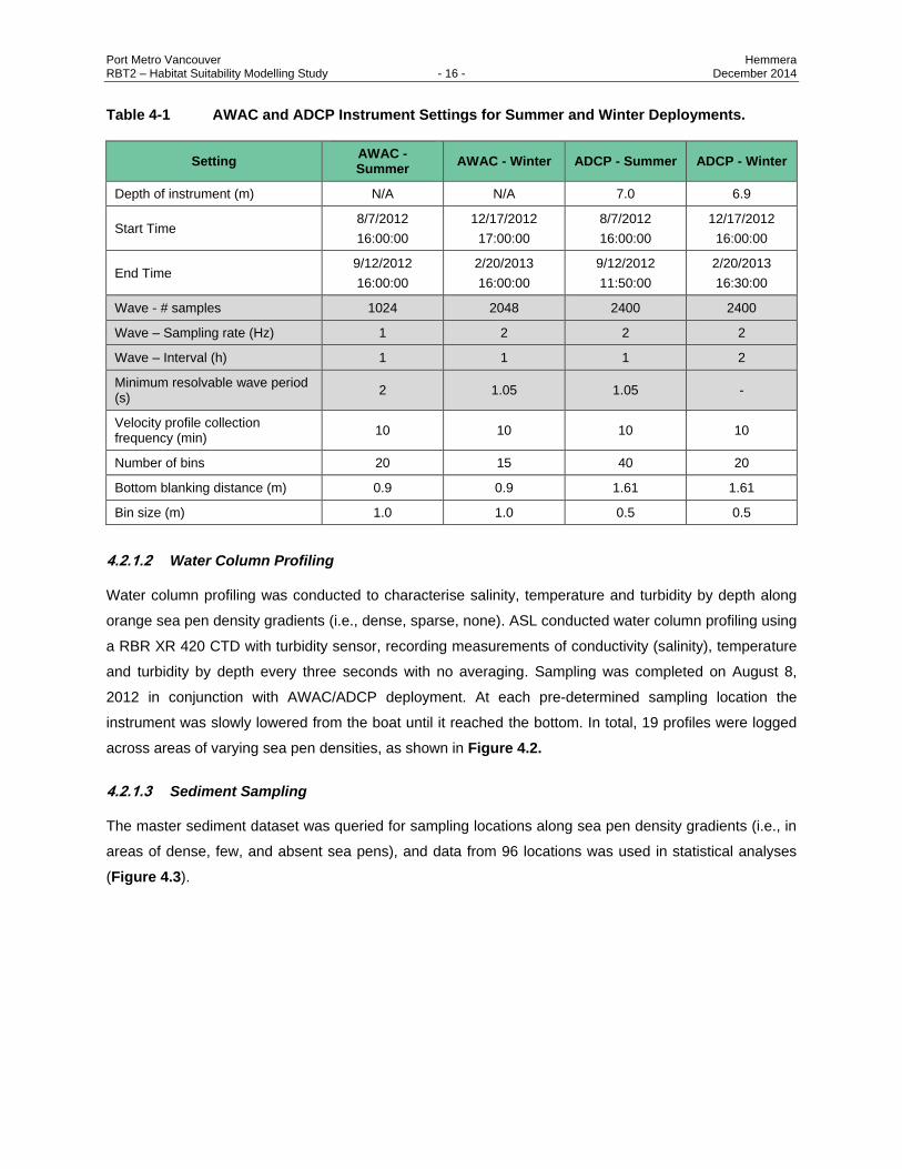
Table 4-1 AWAC and ADCP Instrument Settings for Summer and Winter Deployments.
Setting AWAC - Summer
AWAC - Winter ADCP - Summer ADCP - Winter
Depth of instrument (m) N/A N/A 7.0 6.9
Start Time 8/7/2012
16:00:00
12/17/2012
17:00:00
8/7/2012
16:00:00
12/17/2012
16:00:00
End Time 9/12/2012
16:00:00
2/20/2013
16:00:00
9/12/2012
11:50:00
2/20/2013
16:30:00
Wave - # samples 1024 2048 2400 2400
Wave – Sampling rate (Hz) 1 2 2 2
Wave – Interval (h) 1 1 1 2
Minimum resolvable wave period (s)
2 1.05 1.05 -
Velocity profile collection frequency (min)
10 10 10 10
Number of bins 20 15 40 20
Bottom blanking distance (m) 0.9 0.9 1.61 1.61
Bin size (m) 1.0 1.0 0.5 0.5
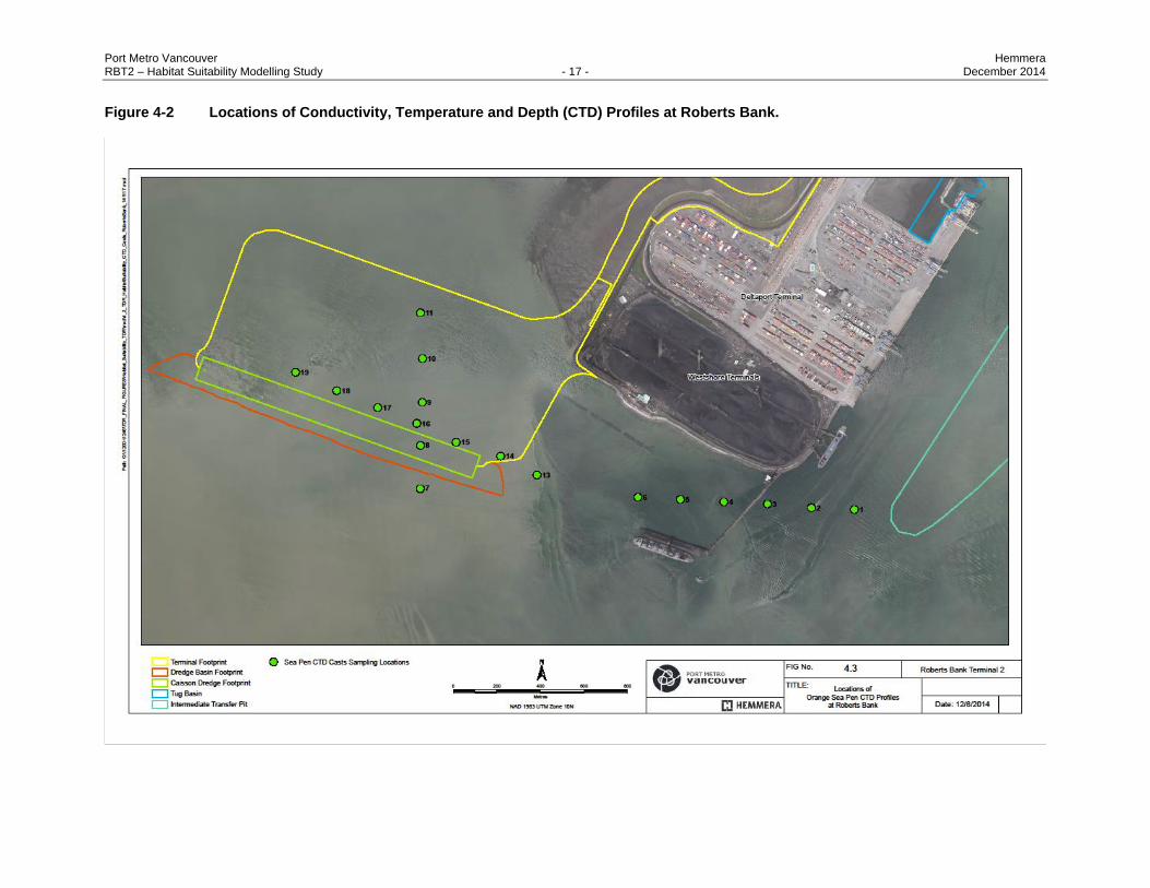
4.2.1.2 Water Column Profiling
Water column profiling was conducted to characterise salinity, temperature and turbidity by depth along
orange sea pen density gradients (i.e., dense, sparse, none). ASL conducted water column profiling using
a RBR XR 420 CTD with turbidity sensor, recording measurements of conductivity (salinity), temperature
and turbidity by depth every three seconds with no averaging. Sampling was completed on August 8,
2012 in conjunction with AWAC/ADCP deployment. At each pre-determined sampling location the
instrument was slowly lowered from the boat until it reached the bottom. In total, 19 profiles were logged
across areas of varying sea pen densities, as shown in Figure 4.2.
4.2.1.3 Sediment Sampling
The master sediment dataset was queried for sampling locations along sea pen density gradients (i.e., in
areas of dense, few, and absent sea pens), and data from 96 locations was used in statistical analyses
(Figure 4.3).
Port Metro Vancouver Hemmera RBT2 – Habitat Suitability Modelling Study - 17 - December 2014
Figure 4-2 Locations of Conductivity, Temperature and Depth (CTD) Profiles at Roberts Bank.

Port Metro Vancouver Hemmera RBT2 – Habitat Suitability Modelling Study - 18 - December 2014
Figure 4-3 Sediment Sampling Locations at Roberts Bank used in Orange Sea Pen Statistical Analyses

Port Metro Vancouver Hemmera RBT2 – Habitat Suitability Modelling Study - 19 - December 2014
All sediment samples were analysed by ALS Environmental in Burnaby, B.C. Raw data are presented in
Appendix C. Univariate statistical analyses were performed using the open source software package R.
4.3 RESULTS
4.3.1 Current Profiling
Time series of current magnitude and direction for a large tide period at approximately 2.4 m above the
bed are plotted for comparison in Figure 4.4. Stage (tide height) is also shown. Current direction is
controlled by the tide condition, with westward flooding currents and eastward ebbing currents. The large
tide was selected for a snapshot as large fluctuations in current velocity are expected, which would tend
to amplify any differences between the two sites.
Current velocities at the dense sea pen (i.e., ADCP) site averaged 0.256 m/s, and averaged 0.247 m/s at
the patchy sea pen (i.e., AWAC) site; this implies that, on average, current velocities are about 4 % higher
in the area of dense sea pens. Separating out deployments by season, velocities from the dense sea pen
site were 11% higher than the patchy site in the summer, but no difference was observed in the winter
record. A maximum velocity of 0.98 m/s was measured at the patchy site on January 12th, 2013 at 03:20,
corresponding to a rising tide. Maximum velocity measured at the dense site over the full period of record
in this second bin is 0.93 m/s on August 18th, 2012 at 14:10, also a rising tide condition.
Figure 4-4 Example of AWAC and ADCP Near-Bed Currents (Magnitude and Direction) for a Large Tide Period from January 7th to January 11th, 2013.
Port Metro Vancouver Hemmera RBT2 – Habitat Suitability Modelling Study - 20 - December 2014
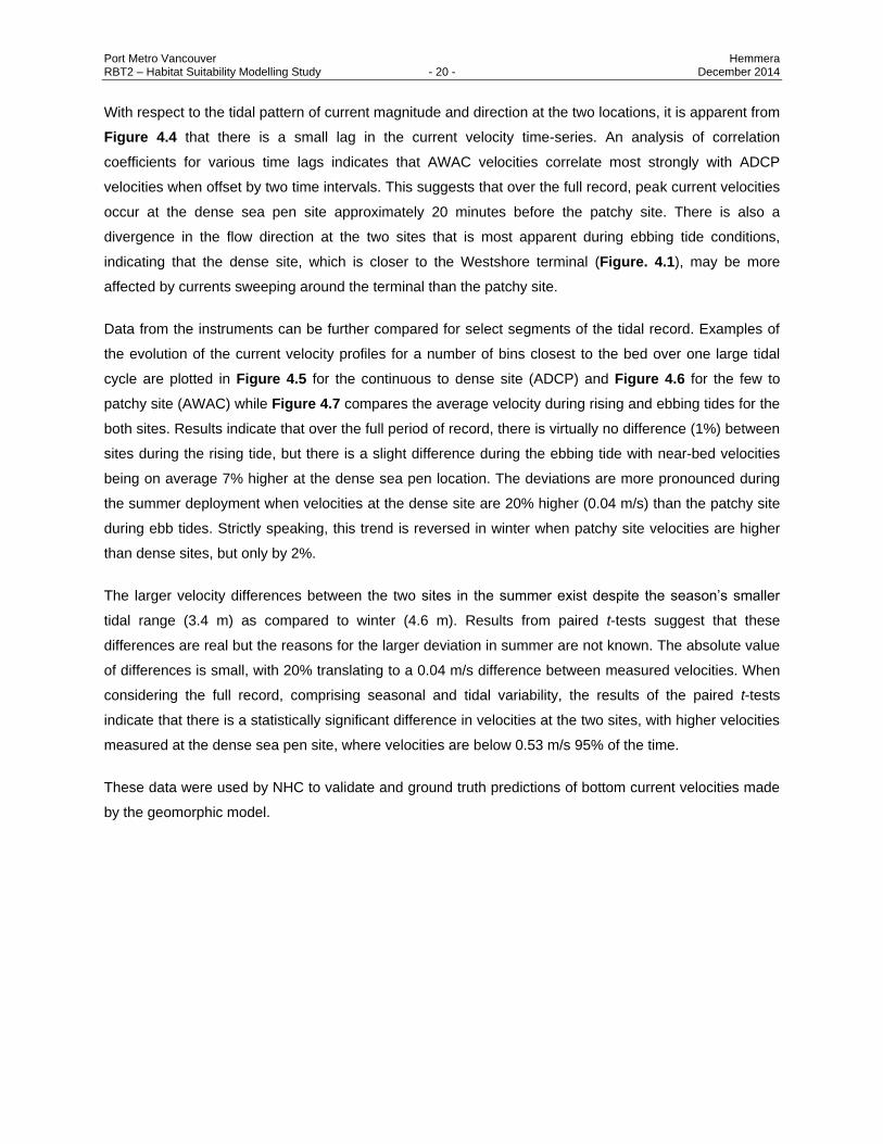
With respect to the tidal pattern of current magnitude and direction at the two locations, it is apparent from
Figure 4.4 that there is a small lag in the current velocity time-series. An analysis of correlation
coefficients for various time lags indicates that AWAC velocities correlate most strongly with ADCP
velocities when offset by two time intervals. This suggests that over the full record, peak current velocities
occur at the dense sea pen site approximately 20 minutes before the patchy site. There is also a
divergence in the flow direction at the two sites that is most apparent during ebbing tide conditions,
indicating that the dense site, which is closer to the Westshore terminal (Figure. 4.1), may be more
affected by currents sweeping around the terminal than the patchy site.
Data from the instruments can be further compared for select segments of the tidal record. Examples of
the evolution of the current velocity profiles for a number of bins closest to the bed over one large tidal
cycle are plotted in Figure 4.5 for the continuous to dense site (ADCP) and Figure 4.6 for the few to
patchy site (AWAC) while Figure 4.7 compares the average velocity during rising and ebbing tides for the
both sites. Results indicate that over the full period of record, there is virtually no difference (1%) between
sites during the rising tide, but there is a slight difference during the ebbing tide with near-bed velocities
being on average 7% higher at the dense sea pen location. The deviations are more pronounced during
the summer deployment when velocities at the dense site are 20% higher (0.04 m/s) than the patchy site
during ebb tides. Strictly speaking, this trend is reversed in winter when patchy site velocities are higher
than dense sites, but only by 2%.
The larger velocity differences between the two sites in the summer exist despite the season’s smaller
tidal range (3.4 m) as compared to winter (4.6 m). Results from paired t-tests suggest that these
differences are real but the reasons for the larger deviation in summer are not known. The absolute value
of differences is small, with 20% translating to a 0.04 m/s difference between measured velocities. When
considering the full record, comprising seasonal and tidal variability, the results of the paired t-tests
indicate that there is a statistically significant difference in velocities at the two sites, with higher velocities
measured at the dense sea pen site, where velocities are below 0.53 m/s 95% of the time.
These data were used by NHC to validate and ground truth predictions of bottom current velocities made
by the geomorphic model.

Port Metro Vancouver Hemmera RBT2 – Habitat Suitability Modelling Study - 21 - December 2014
Figure 4-5 ADCP Profiles over the First Five Bins (up to 4.11 m above the bed) for One Tide Cycle (January 11th-12th). Note that a zero velocity was assumed for the bed.
Figure 4-6 AWAC Profiles over the First Three Bins (up to 3.9 m above the bed) for One Tide Cycle (January 11th-12th). Note that a zero velocity was assumed for the bed.

Port Metro Vancouver Hemmera RBT2 – Habitat Suitability Modelling Study - 22 - December 2014
Figure 4-7 Average Velocity at 2.4 m Above the Bed During Rising Tide and Ebbing Tide for AWAC and ADCP for the Full Period of Record.
4.3.2 Wave Profiling
Wave heights recorded at the dense and patchy sea pen sites over the full period of record are
comparable, with mean values slightly higher at the dense site (0.23 m) than the patchy site (0.20 m)
(Figure 4.8).
In addition to a greater tidal range, the effect of storm events can also be observed in the data record
from the winter deployment (Figure 4.9). A large storm occurred on December 19th, 2012, and peak
wave heights during the event were 1.63 m at the patchy site and 1.73 m at the dense site, respectively.
Maximum current velocities during the storm were high: 0.66 m/s at the dense site and 0.75 m/s at the
patchy site. However, the storm also coincided with large tides, making it difficult to separate out the
influence of waves. In subsequent days, comparable current velocities were achieved when large waves
were absent but tides were large (Figure 4.9). This suggests that large tidal swings have a greater effect
on velocities close to the bed than large wave events. This is not unexpected given that for waves, water
particle displacements and velocities decrease with distance from the surface.
0.00
0.10
0.20
0.30
0.40
Rising tide Ebbing tide All
Ave
rag
e v
elo
cit
y (
m/s
)
Average AWACvelocity (2.4m)
Average ADCP velocity(2.34m)

Port Metro Vancouver Hemmera RBT2 – Habitat Suitability Modelling Study - 23 - December 2014
Figure 4-8 Characteristic Wave Heights at Patchy (AWAC) and dense (ADCP) Orange Sea Pen Sites over the Full Period of Record.
Figure 4-9 Wave Heights, Tide Levels and Near-Bed Current Velocities at Patchy (AWAC) and Dense (ADCP) Orange Sea Pen Sites During a Large Storm Event on December 19th, 2012 and Subsequent Days.
0
0.1
0.2
0.3
0.4
0.5
AWAC ADCP
Heig
ht
(m)
max height
mean 1/10 height
significant wave height
Port Metro Vancouver Hemmera RBT2 – Habitat Suitability Modelling Study - 24 - December 2014
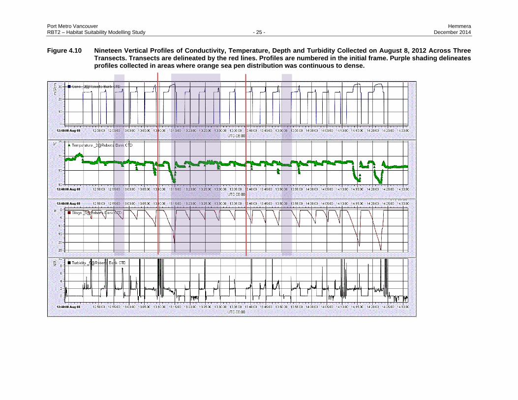
4.3.3 Water Column Profiling
With respect to other abiotic parameters, nineteen vertical profiles of conductivity, temperature, depth
(CTD) and turbidity were collected on August 8th, 2012 across three transects (Figure 4.10). Profiles that
are wholly located in dense sea pen beds were isolated and briefly compared to those in patchy sea pen
areas. No apparent differences were noted in conductivity, temperature or turbidity between the two sea
pen distribution categories, but further analysis may be merited.
Port Metro Vancouver Hemmera RBT2 – Habitat Suitability Modelling Study - 25 - December 2014
Figure 4.10 Nineteen Vertical Profiles of Conductivity, Temperature, Depth and Turbidity Collected on August 8, 2012 Across Three Transects. Transects are delineated by the red lines. Profiles are numbered in the initial frame. Purple shading delineates profiles collected in areas where orange sea pen distribution was continuous to dense.

Port Metro Vancouver Hemmera RBT2 – Habitat Suitability Modelling Study - 26 - December 2014
4.3.4 Sediment Characteristic
Mean sediment grain size was compared across the sea pen density gradient, at sites of dense, patchy
and absent sea pens using non-parametric Wilcoxan rank sum tests. Results for the various size fractions
all followed the same trend: there were significant differences in grain size between samples collected
from sites with dense sea pen aggregations and samples from those sites with either patchy or no sea
pens. There was not a significant difference in sediment texture between sites with patchy aggregations
and those with no sea pens (Table 4.2 and Figure 4.10). These results suggest that the density of sea
pens is inversely correlated with proportion of the seabed as percent fines (i.e., silt and clay).
Table 4-2 Comparison of Geometric Mean Sediment Grain Size Composition (%) Among Sites.
Site Mean % Sand Mean % Silt Mean % Clay Geometric Mean
Absent 83.95 11.42 3.25 0.18
Patchy 81.37 11.71 3.45 0.17
Dense 96.16 1.74 0.66 0.33
Figure 4-10 Percent Sediment (Sand, Clay, Silt and Gravel) Associated with Areas of Dense, Patchily-Distributed (‘Patchy’), and No Orange Sea Pens

Port Metro Vancouver Hemmera RBT2 – Habitat Suitability Modelling Study - 27 - December 2014
4.3.5 Species Distribution Model Development
A Species Distribution Modeling (SDM) approach was used for orange sea pens using generalised linear
models (GLMs) to describe the relationship between sea pen occurrence and environmental parameters.
GLMs are capable of using data from a number of different probability distributions providing the flexibility
needed when using observational ecological data (Guisan et al. 2002). In this case, a logistic regression
GLM was created using georeferenced orange sea pen presence/absence data as the dependent
variable, as a function of environmental variables (bottom current velocity, wave height, sediment grain
size, depth, and both broad and fine scale BPI (Bathymetric Position Index).
A total of 34,555 data points were included in the orange sea pen dataset: 16,457 absence points and
18,098 presence points. Points along transects where orange sea pens were not observed were treated
as absence points. Data points were then separated into a “training” data set used to develop the SDM,
and “evaluation” data set used to assess the predictive accuracy of the model. Seventy percent (70%) of
the presence and absence points were randomly selected for use in model development (i.e., training)
while the remaining 30% were set aside for assessing the accuracy of model predictions (i.e., evaluation).
Each abiotic raster (e.g., slope, depth, bottom current velocity) was used to create a full model with all
parameters. The training dataset (i.e., all orange sea pen presence-absence locations) was then used to
generate a series of plausible models. A backwards stepwise regression analysis, guided by Akaike’s
information criterion (AIC), was used to determine the “best fit” multiple linear regression model (Posada
and Buckley 2004) for the suite of candidate predictor variables. This process typically involves adding or
removing variables and assessing how the model performs. A model with too many variables will have
very high precision but poor predictive power for the general system of interest (being overly specified to
the specific data used in the regression analysis), whereas a model with too few variables may be biased
with its predictive accuracy undermined by potentially spurious correlations (Burnham and Anderson
2002). Model selection, validation, and predictions were performed using Marine Geospatial Ecological
Tools (MGET) within ArcGIS and integrated with the R statistical package (R Development Core Team
2014). During model selection, both broad and fine scale BPI, bottom current velocity, and wave height
were kept in the model, while sediment size distribution and depth were excluded. Depth was excluded
due to highly collinearity with most of the other variable considered in the model. Sediment size
distribution was excluded as it did not improve the models ability to describe the dependent variable (sea
pen presence).
The best fit model was then used to predict the probability of sea pen occurrence for unsampled
locations, to produce a generalised raster of predicted distribution in the study area, and through use of a
binomial logistic regression model (Guisan et al. 2002). The best fit model subsequently was tested for its
predictive capabilities by comparing the predicted occurrence of orange sea pens to the evaluation
dataset (i.e., the 30% of the observational data not used in the creation of the model).

Port Metro Vancouver Hemmera RBT2 – Habitat Suitability Modelling Study - 28 - December 2014
Two methods were used to test model accuracy. Cohen’s kappa values were calculated to determine
agreement between predicted and observed presence and absence values, using the evaluation data
against the predictive raster created using the training data. Cohen’s kappa is similar to percent
agreement but is more robust in that accounts for agreement occurring by chance (Cohen 1960). The
second approach the area under the receiver operating characteristic curve (AUC) was calculated for the
GLM. AUC is used to estimate the probability that randomly chosen observations of species occurrence
would be assigned a higher ranked prediction than a randomly chosen absence observation.
A binary predicted presence/absence raster was derived from the probability of occurrence raster by
setting a threshold probability of 0.55. This value was chosen because it is within the 0.5 to 0.7 range
which is commonly used in published GLM studies (Austin 1998, Hirzel and Guisan 2002). The binary
raster displays predicted presence/absence of sea pens; where ‘0’ or unsuitable habitat classification is
the predicted probability of occurrence at <0.55 and ‘1’ or suitable habitat classification >0.55. To further
delineate habitat suitability the suitable habitat classification was delineated at >0.55, <0.8 as moderate
suitability and >0.8 as highly suitable habitat, for a total of three habitat suitability classifications.
An area along the subtidal slope was masked from the final results, as it encompasses subtidal channels
that have obvious geomorphic patterns consistent with sediment slumping and slope failure. It was
hypothesised that the lack of sea pen sightings in this region is likely due physical disturbance caused by
extensive channelisation.
NHC’s coastal geomorphology model considers environmental parameters under two scenarios: one
without the Project and one with the Project. The orange sea pen SDM was used to map sea pen habitat
for each scenario, producing two predictive habitat suitability maps.
4.4 SDM OUTPUTS
As expected, the GLM for orange sea pens predicted the highest probability of occurrence along fore-
slope shallow subtidal habitats (Figure 4.11). Comparison of the evaluation data set to model predictions
resulted in 74 % positive prediction value for presence and 87 % negative prediction value for absence
locations. The overall accuracy of the model was 79 % with a statistically significant Cohen’s Kappa
(KHAT) value of 0.57 (p < 0.000). A KHAT value between 0.41 and 0.60 signifies a ‘moderate’ agreement
(Landis and Koch 1977). An AUC value of 0.85 suggest an significant improvement over a random
classifier (AUC 0.5). Values of AUC above 0.7 is an acceptable level of performance, between 0.8 and
0.9 is excellent, above 0.9 is outstanding, and an AUC value of 1 would be a perfect classifier (Hosmer
and Lemeshow 2004).

Port Metro Vancouver Hemmera RBT2 – Habitat Suitability Modelling Study - 29 - December 2014
Stepwise AIC analysis found bottom current velocity, wave height, broad BPI, and fine BPI to be
significant factors in predicting the distribution of orange seapens (Table A1, Appendix A). The equation
for the model based on the coefficients is:
GLM = -9.284 - [(6.907) × ubot] + [(17.794) × wave height] – [(1.783e-1) × broad BPI] + [(6.495e–1) × fine
BPI]
Under existing conditions, the SDM identified 318.4 ha of suitable (>0.55) orange sea pen habitat within
the modelled area at Roberts Bank, of which 110.5 ha is high suitability and 207.9 ha is moderate
suitability habitat (Figure 4.11, Table 4.3). With development of RBT2, 86.1 ha (27%) of suitable (i.e.,
high + moderate suitability) orange sea pen habitat will be directly displaced by placement of Project
components, leaving ~232.3 ha of habitat suitable for orange sea pens available at Roberts Bank. A net
gain (3.4 ha) in the amount of high suitability habitat is predicted. (Figure 4.11, Table 4.3).
Table 4-3 Habitat Suitability (ha) for Orange Sea Pens (Ptilosarcus gurneyi) in Future Scenarios With and Without RBT2.
Suitability Ranking Without RBT2 (ha) With RBT2 (ha) Loss (-)/Gain (+) (ha)
High Suitability (>0.8) 110.5 113.9 +3.4
Moderate Suitability (0.55 – 0.8) 207.9 118.4 - 89.5
Low Suitability (<0.55) 5110.8 5017.2 -93.6
Total 5429.1 5249.5 -179.6
4.5 DISCUSSION
The best fit model for orange sea pens included four environmental variables: bottom current velocity,
wave height, and both broad and fine scale BPI. Several predictor variables were rejected in the model
development, including sediment texture indicator variables and seabed depth. Use of the AIC to define
the “best fit” model helps to maximise the predictive power based on the smallest number of predictor
variables and, therefore, results in exclusion from the model of variables that are either poorly associated
with the dependent variable (sea pen presence or absence) or are highly correlated with other predictor
variables included in the model. In this case, sediment grain size was excluded from the model; however,
it was considered indirectly, as bottom current velocity and wave height can be considered proxies for
sediment grain size distribution (as minimum speeds are required to induce sediment transport). Including
both velocity and grain size as parameters may result in collinearity1, which may introduce noise and
affect overall model precision (i.e., larger standard errors in the related independent variables).
1 Collinearity is a statistical phenomenon in which two or more predictor variables are highly correlated, meaning that one can be
linearly predicted from the others with a high degree of accuracy.

Port Metro Vancouver Hemmera RBT2 – Habitat Suitability Modelling Study - 30 - December 2014
Under existing conditions, the HSM indicates that 318.4 ha of suitable (i.e., high plus moderate suitability)
orange sea pen habitat exists at Roberts Bank. Towed underwater video surveys of the area have
resulted in the mapping 174 ha of orange sea pen distribution, -23 ha of which supports continuous to
dense aggregations, while 151 ha supports sparse and patchy aggregations. Taken together, this implies
that orange sea pens are not currently exploiting the full range of available high quality habitat as
suggested by the HSM.
A total of 86.1 ha, or 27%, of suitable orange sea pen habitat is predicted to be lost to RBT2 construction
(Table 4.3, Figure 4.11B). However, this value is driven by the loss of moderate suitability habitat, as the
model predicts a net increase of highly suitable habitat (3.4 ha, or 1%). The increase results from
moderate suitability habitat increasing to high suitability habitat in localised areas around the terminal.

Port Metro Vancouver Hemmera RBT2 – Habitat Suitability Modelling Study - 31 - December 2014
Figure 4-11 Habitat Suitability for Orange Sea Pens at Roberts Bank, as Identified by the Species Distribution Model, A) Without RBT2 (Existing Conditions), and B) With RBT2.
Port Metro Vancouver Hemmera RBT2 – Habitat Suitability Modelling Study - 32 - December 2014
Under existing conditions, orange sea pens are clustered around the edges of the Westshore Terminal
(Figure 4.1), likely because flow accelerates as water moves around the structure, thereby increasing
food delivery to sea pens (Section 4.2.1 above; Hemmera 2014). The model predicts that RBT2 will
create similar favourable feeding conditions at its edges (Figure 4.11), which may attract sea pens back
to the area over time; however, rates of recovery are unknown as re-colonisation may be subject to
density-dependent limitations.
Loss of orange sea pens from Roberts Bank would potentially reduce habitat structural complexity that
supports other species, such as fish and macroinvertebrates that favour emergent structures (e.g.,
juvenile flatfish) (Stoner et al. 2007). Orange sea pens are also ecologically important as a prey species
in supporting a number of predators, including several species of sea stars and nudibranchs (Birkeland
1974). Large aggregations of sea pens are considered habitats suitable for the establishment of diverse
benthic communities and are becoming recognised as important habitat for both fish and invertebrates
(DFO 2011), thereby influencing the overall productivity of the Roberts Bank marine ecosystem.
The SDM approach may be limited by incomplete mapping of orange sea pen occurrence, and not fully
capturing the relationship with environmental parameters. Orange sea pens are commonly found
throughout nearshore subtidal areas, and individual occurrence may be less limited than it is for larger
aggregations such as at Roberts Bank. This difference between the general or local conditions required
by individuals and the larger scale conditions required for aggregations is difficult to discern. No detailed
scientific studies have been completed on upper and lower thresholds with regard to environmental
preferences, and modeled relationships may be insensitive to abrupt shifts in preferences at threshold
levels not adequately modeled. The evaluation of sea pen distributions on a more continuous numerical
scale – for example, as standing stock biomass or based on the abundance of different size classes –
might have facilitated a greater understanding of abiotic and biotic drivers for suitable and optimal habitat.
Finally, the environmental parameters represent a snapshot in time while aggregation patterns of
individuals may result from a broader scale of environmental patterns not reflected in the data
(e.g., based on inter-annual trends and longer term cycles, such as associated with Pacific Decadal and
El Nino Oscillations). Dense aggregations of orange sea pens are not well documented and the
mechanisms facilitating these patterns are poorly understood.
SDMs are only as informative as the data that are input to the model. The orange sea pen SDM included
data for environmental variables that were available as digital surfaces for the study area. The model
variables were chosen based on an understanding of sea pen feeding ecology and extrapolated from
comparisons with ecologically similar species (e.g., corals). Selection of environmental parameters was
also limited by data availability and it is possible that other variables not included in the model are
important to orange sea pen populations at Roberts Bank, or that the SDM did not capture complex and
potentially non-linear interactions between environmental variables that may be important to sea pen

Port Metro Vancouver Hemmera RBT2 – Habitat Suitability Modelling Study - 33 - December 2014
habitat preference or population structure. Additionally, environmental variable data originated from a
number of sources, including the wider literature in addition to field data collected on site (Appendix A).
Literature derived data were not always from the study area, and thus conditions may differ between
Roberts Bank and the study site that the data originated from.
No data on biological interactions were input to the model, thus potentially neglecting complex predator-
prey and competitive species interactions which may influence orange sea pen habitat preference or their
ability to realise such preferences. The SDM does not capture temporal variation, including differences in
annual recruitment and death that affect population dynamics. Studies in Puget Sound, for example,
indicate that larval settlement can be highly episodic in time giving rise to discontinuous populations
differing in age and size (Birkeland 1968, 1974). The orange sea pen presence/absence data on which
the SDM is based may also have missed areas of sea pen be under representative of populations at
Roberts Bank, as individuals retract into the sediment and may not be seen by surveying biologists. For
example, while diving in Puget Sound, Birkeland (1968) observed that only ~26% of the orange sea pens
were exposed at any one time, with the rest buried in the sediment. The SDM is also unable to consider
any influential, non-Project related changes to orange sea pen populations at Roberts Bank, such as
those due to climatic forcing regimes (i.e., El Nino Southern Oscillation, Pacific Decadal Oscillation) or
climate change.
Port Metro Vancouver Hemmera RBT2 – Habitat Suitability Modelling Study - 34 - December 2014
5.0 DUNGENESS CRAB HSM
5.1 REVIEW OF EXISTING LITERATURE AND DATA
5.1.1 Distribution
Dungeness crabs (Metacarcinus magister) are widely distributed along the western continental shelf of
North America, from the Pribolof Islands, Alaska to Santa Barbara, California (Jensen and Armstrong
1987). Dungeness crab populations inhabit shallow coastal waters, such as estuaries, inlets and bays,
although many populations reside in open ocean habitats (Holsman et al. 2003; reviewed by Rasmuson
2013). Because of the widespread distribution of this species, there is spatial and temporal variation in
microhabitat use across different populations (Rasmuson 2013). Therefore, this review focuses on
available information on the abiotic variables influencing Dungeness crab habitat use in northeastern
Pacific estuarine systems.
5.1.2 Habitat Requirements and Limiting Factors
Environmental variables that govern Dungeness crab habitat preferences are similar across life history
stages, but the specific requirements within each environmental variable differ, thus the habitat
preferences of juvenile, adult, and gravid female Dungeness crabs were assessed separately. For
detailed Dungeness crabs life history refer to the Juvenile Dungeness Crab and Dungeness Crab
Productivity Technical Data Reports.
5.1.2.1 Juveniles
Juvenile Dungeness crabs (young-of-the-year; 0+ age class; 5-7 mm carapace width (CW)) rely heavily
on complex estuarine habitats as nurseries (Gunderson et al. 1990, Fernandez et al. 1993, Armstrong et
al. 2003). Like other crustaceans, Dungeness crabs grow by moulting or shedding their shells. Unlike
adult crabs, juveniles grow rapidly, moulting several times during the first two years of growth (reviewed in
Rasmuson 2013). Therefore, the availability of secondary substrate types and the refuge they provide
from predators is correlated with patterns of juvenile survival and abundance (Dumbauld 1993, McMillan
et al. 1995, Rooper et al. 2002).
The importance of estuaries as nursery habitat for juvenile Dungeness crabs has been well documented
(Tasto 1983, Armstrong and Gunderson 1985, Stevens and Armstrong 1985, McMillan et al. 1995).
Recently settled crabs are most abundant in areas associated with secondary microhabitats such as
gravel and rocky substrates covered in macroalgae, and silt or sandy bottoms that support dense
eelgrass beds (McMillan et al. 1995, Rooper et al. 2002, Burd et al. 2008a). Later instar and age 1+ crab
densities are highly correlated with near-shore sub-channels close to the estuary mouth, which are
generally characterised by shallow depths (<10 m), relatively high salinities and lower temperatures
(<18 ºC) (Rooper et al. 2002). Site specific studies corroborate the literature, with UIva and Zostera
japonica identified as the most highly utilised juvenile habitats at Roberts Bank (Triton 2004, Martel 2009,
Hemmera 2014c).
Port Metro Vancouver Hemmera RBT2 – Habitat Suitability Modelling Study - 35 - December 2014
5.1.2.2 Adults
Adult Dungeness crabs (2+ age class) are most abundant on subtidal sand or mud bottoms (Cleaver
1949) and are frequently found inactive and buried in the soft sediment during the day (McGaw 2005).
Adult crabs migrate daily to shallow intertidal flats to forage during nocturnal high tides (Holsman et al.
2006, Curtis and McGaw 2012). Field and laboratory studies suggest that adult crabs display
physiological and behavioral stress responses to low salinity conditions below 24 psu (Curtis and McGaw
2008, 2012) and are unable to tolerate prolonged exposure to salinities below 12 psu (Cleaver 1949).
Therefore, cooler temperatures and higher salinity levels that are associated with high tides allow adults
to enter and exploit shallow sandy-bottom habitats (Curtis and McGaw 2008).
5.1.2.3 Gravid Females
When Dungeness crabs reach sexual maturity at around 2 to 3 years of age (100 mm carapace width),
individuals migrate towards near-shore habitats to copulate (reviewed in Rasmuson 2013). Mating
between a recently moulted (soft-shell) female and an already moulted and hardened male occurs
generally between April to September in Puget Sound (Rasmuson 2013). Although no data on the timing
of copulation is available for British Columbia, fertilised eggs are extruded in approximately October to
March (Rasmuson 2013).
Highly fecund gravid females, each bearing about 2 million fertilised eggs, remain in the shallow water
habitat (<10 m) (Armstrong et al. 1988) and form dense aggregations during the fall and winter
(September-February in British Columbia) (Shirley et al. 1987). Brooding habitats are consistently
characterised by homogeneous sandy substrate that is highly permeable and typically well oxygenated
(Scheding et al. 2001, Stone and O’Clair 2002). Optimal conditions under which eggs develop normally
are suggested to be at a salinity of 25 psu and water temperature of 12ºC (Mayer 1979). Brooding times
range from 65 to 130 days with the shortest durations corresponding to highest water temperatures
(17ºC) and lowest hatching success (Wild 1980). During this time, females must bury themselves into the
sand (5 to 10 cm) to maintain attachment of the eggs to their underside (cephalothorax) (O’Clair et al.
1996). As a result, most brooding females are found partially or completely buried within the sediment,
where movement becomes relatively limited until the eggs are ready to hatch (December-June in British
Columbia) (O’Clair et al. 1996, Scheding et al. 2001, Rasmuson 2013).
Gravid females have also been observed in deeper water (16 m) (Stone and O’Clair 2002). Because
females have been shown to return to the same brooding locations for many years, such combinations of
medium sediment-sized sandy substrates (with or without vegetative cover) and relatively shallow water
depths form habitats for this life history stage (O’Clair et al. 1996, Scheding et al. 2001). Observations of
gravid female crabs in the proposed RBT2 footprint are consistent with previous studies and suggest that
females prefer sandy sediment substrates to brood their eggs. However, no gravid female aggregations
were found in this study area and most individuals observed (75%) inhabited deeper waters (-10 to -20m)

Port Metro Vancouver Hemmera RBT2 – Habitat Suitability Modelling Study - 36 - December 2014
at similar depths reported in northern estuaries (e.g., Alaska) (Stone and O’Clair 2002). Suitable sandy
substrates are often a relatively limited resource in some estuarine systems, particularly in those that are
dominated by muddy intertidal flats at all depth ranges (Scheding et al. 2001). Therefore, habitats for
gravid Dungeness crabs should be considered high management and mitigation priorities during
anthropogenic development (Scheding et al. 2001).
5.2 METHODS FOR DEVELOPMENT OF HSM
A weighted rating HSM was developed for Roberts Bank to indicate areas with potentially suitable habitat
for juvenile, adult, and gravid female Dungeness crabs. Areas of high, moderate, and low habitat
suitability for supporting the three Dungeness crab life stages were identified based on environmental
data from Roberts Bank, combined with literature information citing preferred ranges for each of the
identified habitat variables. Where literature information on Dungeness crab was not available,
preferences were extrapolated from information on other phylogenetically and ecologically related crab
species such as Cancer productus and Cancer gracilis (see Table A1, Appendix A for HSM model input
sources).
Five environmental variables were identified from the literature: 1) water depth, 2) slope, 3) sediment
grain size distribution, 4) salinity, and 5) habitat type (Table A1, Appendix A). Continuously distributed
environmental variables such as depth were divided in a series of four to eight discrete ranges, and each
of these discrete ranges was assigned a suitability index (SI) range between either 1 and 10 in the case
of depth or 0.1 and 1.0 for the other continuous variables, based on literature-derived preference values
and professional judgement. Ranges for each factor and associated SI values are presented in Table 5.1.
Similarly, habitat types were assigned an SI in the range of 0.1 to 1.0. Slope preferences were based on
professional judgement, where flat areas less than 5 degrees slope was high suitability, increasing to
10 degrees slope was moderate suitability, and above 10 degrees slope was low suitability.
An overall habitat suitability range was determined for Dungeness crab at Roberts Bank using a
cumulative scoring technique; i.e. based on an assumed additivity of SI values for the various predictor
variables. Overall habitat suitability scores were derived using ArcGIS 10.2 by overlaying geospatial
representations of the five environmental variables. Each variable had an associated mapped surface for
Roberts Bank, which was used to calculate suitability by reclassifying each variable according to the
suitability index (SI). A weighted factor of 10 was applied to depth as it was determined to be a significant
limiting factor for each group by the model. The weighted rating approach allowed the relative importance
of each variable to more accurately reflect the overall habitat suitability. After the layers were reclassified
to a common scale and weighted, they were added together using the raster algebra tool in ArcGIS for
each HSI model.

Port Metro Vancouver Hemmera RBT2 – Habitat Suitability Modelling Study - 37 - December 2014
Only direct effects of the Project footprint (i.e., terminal and dredge basin) could be modelled, as not all
environmental input variables were available for future scenarios; for example, no predictive data exist for
habitat type and sediment grain size. Therefore, the total area of overlap between the Project footprint
and habitat metrics was calculated, producing estimates of the amount of area of each suitability class
that the Project would cover.
Table 5-1 Environmental Variable Inputs for Dungeness Crab Weighted Rating Habitat Suitability Model (HSM).
Environmental Variable Life History Phase
Adult Gravid Female Juvenile
Water Depth (m) Weight (1 - 10)
2.35 to 3.23 1 1 4
1.47 to 2.35 1 1 8
1.47 to 0.56 4 5 10
0.56 to 0.00 8 5 8
0.00 to -10 10 10 6
-10 to -20 10 10 1
-20 to -30 8 6 1
-30 to -100 6 1 1
Slope Weight (0.1 - 1)
0 - 5 1 1 1
5 - 10 0.6 0.8 0.4
10 - 15 0.1 0.1 0.1
15 - 20 0.1 0.1 0.1
Percent Sand (%) Weight (0.1 - 1)
0 - 30 0.5 0.1 0.6
30 - 40 0.5 0.1 0.6
40 - 50 0.8 0.1 0.8
50 - 60 1 0.1 1
60 - 70 1 0.1 0.1
70 - 80 1 1 1
80 - 90 1 1 0.8
90 - 100 1 1 0.6
Salinity (PSU) Weight (0.1 - 1)
0 - 15 0.1 0.1 0.6
15 - 18 0.2 0.1 0.6
18 - 20 0.2 0.1 0.8
20 - 22 0.2 0.6 0.8
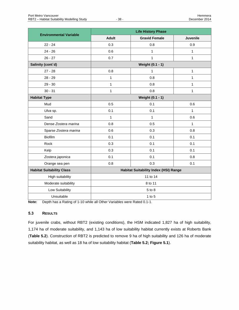
Port Metro Vancouver Hemmera RBT2 – Habitat Suitability Modelling Study - 38 - December 2014
Environmental Variable Life History Phase
Adult Gravid Female Juvenile
22 - 24 0.3 0.8 0.9
24 - 26 0.6 1 1
26 - 27 0.7 1 1
Salinity (cont`d) Weight (0.1 - 1)
27 - 28 0.8 1 1
28 - 29 1 0.8 1
29 - 30 1 0.8 1
30 - 31 1 0.8 1
Habitat Type Weight (0.1 - 1)
Mud 0.5 0.1 0.6
Ulva sp. 0.1 0.1 1
Sand 1 1 0.6
Dense Zostera marina 0.8 0.5 1
Sparse Zostera marina 0.6 0.3 0.8
Biofilm 0.1 0.1 0.1
Rock 0.3 0.1 0.1
Kelp 0.3 0.1 0.1
Zostera japonica 0.1 0.1 0.8
Orange sea pen 0.8 0.3 0.1
Habitat Suitability Class Habitat Suitability Index (HSI) Range
High suitability 11 to 14
Moderate suitability 8 to 11
Low Suitability 5 to 8
Unsuitable 1 to 5
Note: Depth has a Rating of 1-10 while all Other Variables were Rated 0.1-1.
5.3 RESULTS
For juvenile crabs, without RBT2 (existing conditions), the HSM indicated 1,827 ha of high suitability,
1,174 ha of moderate suitability, and 1,143 ha of low suitability habitat currently exists at Roberts Bank
(Table 5.2). Construction of RBT2 is predicted to remove 9 ha of high suitability and 126 ha of moderate
suitability habitat, as well as 18 ha of low suitability habitat (Table 5.2; Figure 5.1).
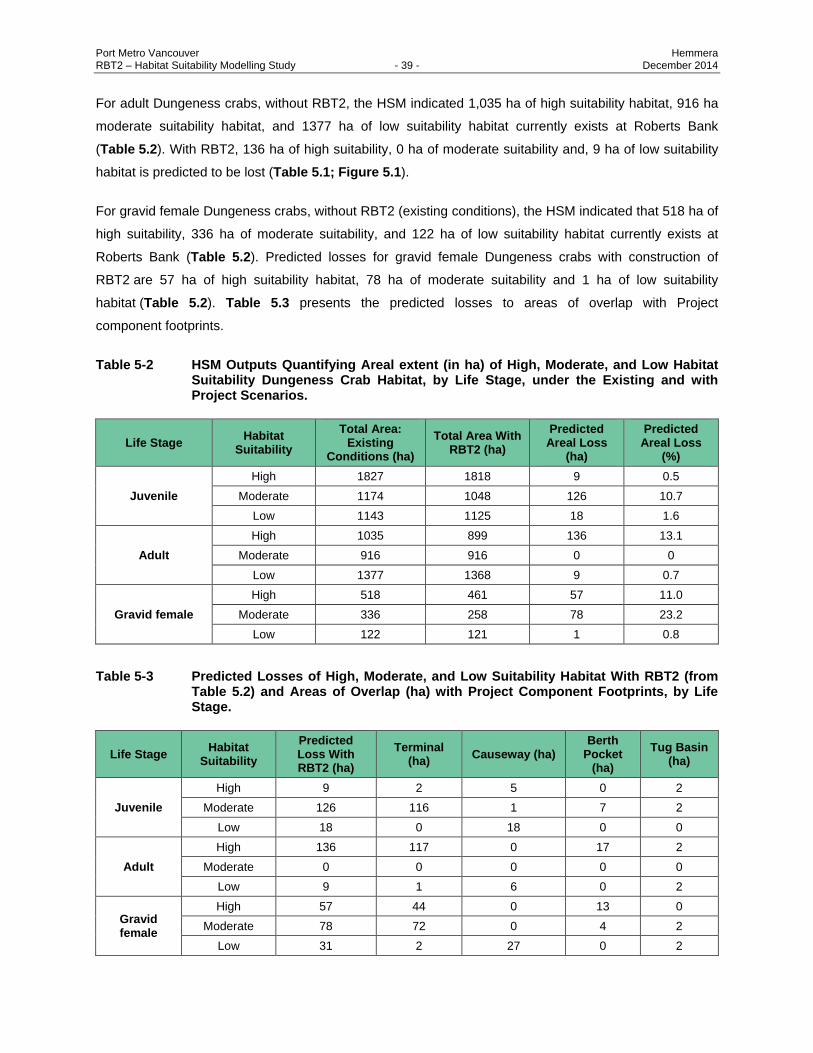
Port Metro Vancouver Hemmera RBT2 – Habitat Suitability Modelling Study - 39 - December 2014
For adult Dungeness crabs, without RBT2, the HSM indicated 1,035 ha of high suitability habitat, 916 ha
moderate suitability habitat, and 1377 ha of low suitability habitat currently exists at Roberts Bank
(Table 5.2). With RBT2, 136 ha of high suitability, 0 ha of moderate suitability and, 9 ha of low suitability
habitat is predicted to be lost (Table 5.1; Figure 5.1).
For gravid female Dungeness crabs, without RBT2 (existing conditions), the HSM indicated that 518 ha of
high suitability, 336 ha of moderate suitability, and 122 ha of low suitability habitat currently exists at
Roberts Bank (Table 5.2). Predicted losses for gravid female Dungeness crabs with construction of
RBT2 are 57 ha of high suitability habitat, 78 ha of moderate suitability and 1 ha of low suitability
habitat (Table 5.2). Table 5.3 presents the predicted losses to areas of overlap with Project
component footprints.
Table 5-2 HSM Outputs Quantifying Areal extent (in ha) of High, Moderate, and Low Habitat Suitability Dungeness Crab Habitat, by Life Stage, under the Existing and with Project Scenarios.
Life Stage Habitat
Suitability
Total Area: Existing
Conditions (ha)
Total Area With RBT2 (ha)
Predicted Areal Loss
(ha)
Predicted Areal Loss
(%)
Juvenile
High 1827 1818 9 0.5
Moderate 1174 1048 126 10.7
Low 1143 1125 18 1.6
Adult
High 1035 899 136 13.1
Moderate 916 916 0 0
Low 1377 1368 9 0.7
Gravid female
High 518 461 57 11.0
Moderate 336 258 78 23.2
Low 122 121 1 0.8
Table 5-3 Predicted Losses of High, Moderate, and Low Suitability Habitat With RBT2 (from Table 5.2) and Areas of Overlap (ha) with Project Component Footprints, by Life Stage.
Life Stage Habitat
Suitability
Predicted Loss With RBT2 (ha)
Terminal (ha)
Causeway (ha) Berth
Pocket (ha)
Tug Basin (ha)
Juvenile
High 9 2 5 0 2
Moderate 126 116 1 7 2
Low 18 0 18 0 0
Adult
High 136 117 0 17 2
Moderate 0 0 0 0 0
Low 9 1 6 0 2
Gravid female
High 57 44 0 13 0
Moderate 78 72 0 4 2
Low 31 2 27 0 2
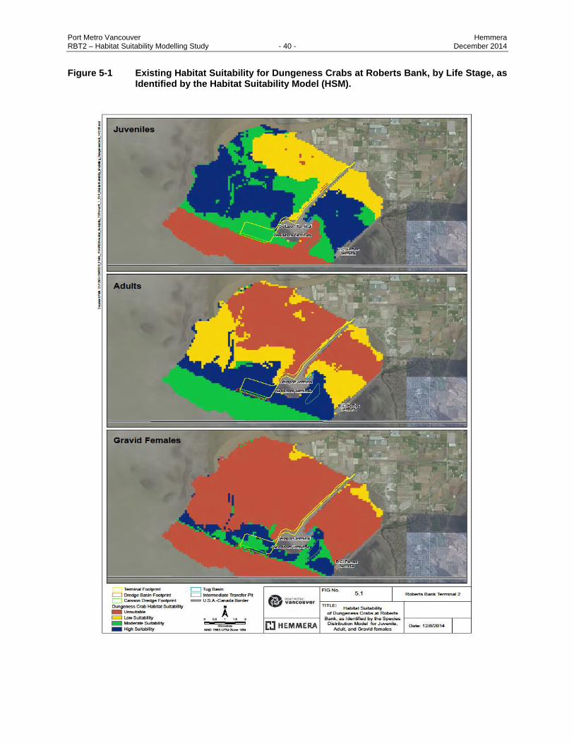
Port Metro Vancouver Hemmera RBT2 – Habitat Suitability Modelling Study - 40 - December 2014
Figure 5-1 Existing Habitat Suitability for Dungeness Crabs at Roberts Bank, by Life Stage, as Identified by the Habitat Suitability Model (HSM).

Port Metro Vancouver Hemmera RBT2 – Habitat Suitability Modelling Study - 41 - December 2014
5.4 DISCUSSION
This study quantified amounts of suitable Dungeness crab habitat at Roberts Bank and results indicate
that, even with projected losses from the RBT2 footprint, >87% high suitability habitat remains for adult
Dungeness crabs, the life stage predicted to be most affected (Table 5.2).
Adult crabs are predicted to be most affected by terminal placement, losing approximately 13% (136 ha)
high suitability habitat (Table 5.2; Figure 5.1B). Field observations of adult Dungeness crabs at Roberts
Bank verify they are highly abundant and broadly distributed, across depths and sediment types. While
some crabs may be permanently displaced by the Project, they are highly mobile and capable of moving
to the high suitability habitat that exists in close proximity, making them less susceptible to localised
habitat changes than juveniles or gravid females and possibly alleviating the impacts of concentrated
habitat loss.
Model results indicate that, of all the life stages, juvenile Dungeness crabs have the greatest amount of
high suitability habitat available at Roberts Bank under existing conditions (1,827 ha; Table 5.2),
suggesting that Roberts Bank may be more important as a nursery habitat to juvenile life stages of
Dungeness crabs than habitat for adults. This is consistent with previous studies, which highlight the
importance of Roberts Bank, and estuaries in general, for the rearing and development of juvenile crabs
(Armstrong and Gunderson 1985, Armstrong et al. 2003, Curtis and McGaw 2008, Martel 2009).
Presence of vast amounts of high quality habitat is expected to remain even after RBT2 construction, as
the terminal’s placement entirely in subtidal waters results in little spatial overlap with juvenile habitat.
Information on the spatial extent and distribution of suitable coarse sand habitat for gravid females is
especially important, because of high habitat specificity and site fidelity associated with this life stage.
Female Dungeness crabs have been shown to return to the same brooding locations annually (Stone and
O’Clair 2002), suggesting habitats relating to sensitive brooding life history stage should be considered
high mitigation priorities (Scheding et al. 2001). Gravid female Dungeness crabs currently have the least
amount of high suitability habitat available to them at Roberts Bank (518 ha), 11% of which is predicted to
be lost to the Project footprint (Table 5.2). However, lack of suitable brooding habitat for gravid female
Dungeness crabs may not affect population structure of subsequent life history stages at Roberts Bank
because Dungeness crabs are considered a metapopulation, sustained by larvae originating over a large
geographical area; therefore, a stock/recruitment relationship is difficult to demonstrate considering the
wide range of potential donors to the larval pool (Zhang et al. 2004).
While SCUBA surveys, ROV video observations, and quantitative sediment grab analyses at Roberts
Bank indicated appropriate sediment for burying by gravid females (refer to the Marine Subtidal Benthic
Technical Data Report), it is also possible that other habitat characteristics may be limiting or that habitat
preferences of individuals at Roberts Bank differ from those presented in the literature.
Port Metro Vancouver Hemmera RBT2 – Habitat Suitability Modelling Study - 42 - December 2014
6.0 PACIFIC SAND LANCE HSM
6.1 REVIEW OF EXISTING LITERATURE AND DATA
6.1.1 Distribution
Pacific sand lance (PSL) (Ammodytes hexapterus) is a small but abundant schooling fish occurring in
estuarine and marine ecosystems throughout the Pacific Northwest (Robards et al. 1999). Ranging from
northern Alaska to southern California, in intertidal waters to depths of approximately -100 m CD (Lamb
and Hanby 2005), this species is considered a key forage fish species in the Salish Sea (Willson et al.
1999, Therriault et al. 2009) and an important prey item for a wide variety of birds, fish, and marine and
terrestrial mammals (Shepherd 1988, Robards et al. 1999).
Despite its ecosystem importance, comprehensive, quantitative data on spatial and temporal patterns in
abundance of Pacific sand lance are lacking (Therriault et al. 2009, Robinson et al. 2013), in part due to
the complex benthic-pelagic life history of this species. Studies in British Columbia, along southwestern
Vancouver Island (Haynes et al. 2007) including Barkley Sound (Haynes 2006, Haynes et al. 2008), have
documented seasonal schools of juvenile and adult Pacific sand lance in shallow intertidal and subtidal
habitats during spring and summer months. Schools have also been observed in eelgrass habitats during
the summer in other regions of British Columbia, including the Gulf Islands, Haida Gwaii, and Clayoquot
Sound (Robinson and Yakimishyn 2013).
Winter months are thought to be primarily periods of near dormancy when sand lance burrow in benthic
substrates (Healy 1984, O’Connell and Fives 1995, Robards and Piatt 1999). Emergence occurs in winter
between November and February from Washington to Alaska, when spawning typically occurs on upper
intertidal beaches (Thuringer 2004, de Graaf 2007, Penttila 2007). Along the Pacific coast, spawning has
been documented in Puget Sound and the San Juan Islands in Washington State (Penttila 1995, 2000,
2007), and to a lesser extent in regions of southern Vancouver Island (Thuringer 2004) and the lower
mainland (de Graaf 2007, CMN 2013).
At Roberts Bank, Pacific sand lance have historically been observed in eelgrass habitat between April
and November, with higher abundances recorded in spring, summer, and early fall in the early 1980s
(Conlin et al. 1982). Sand lance have been caught in beach seine and trawl nets in numerous habitat
types in the vicinity of Deltaport. (Triton 2004, Archipelago 2014a, b, c, Hemmera 2014d). In recent
surveys at Roberts Bank, young-of-the-year (YOY) Pacific sand lance, (i.e., less than 90 mm fork length)
(Field 1988, Robards et al. 2002) were caught in the eelgrass bed and mud flats north of the causeway in
the spring and summer of 2012 (n = 31 total) (Archipelago 2014b). Nine Pacific sand lance were caught in
winter 2012/2013 in a single tow within the -5 to -10 m depth CD zone, the majority of which were also
YOY (Archipelago 2014a). While these observations confirm the presence of sand lance in the nearshore
of Roberts Bank, it is difficult to directly correlate presence of these species in the water column with
Port Metro Vancouver Hemmera RBT2 – Habitat Suitability Modelling Study - 43 - December 2014
suitable spawning and burying habitat. Sand lance will move from suitable sandy refuges to feed, with
farther movements offshore occurring during daylight foraging hours (Kühlmann and Karst 1967, van der
Kooij et al. 2008).
6.1.2 Habitat Requirements and Limiting Factors
Pacific sand lance are considered a critical link in the food chain along with other forage fish species,
between zooplankton prey and top marine predators, such as piscivorous fishes, seabirds and marine
mammals that consume it (Robards et al. 1999, Haynes et al. 2007, Johnson et al. 2008, Therriault et al.
2009). At Roberts Bank, schools of Pacific sand lance are likely consumed by species as varied as
pelagic cormorants, gulls, harbor seals (Phoca vitulina), Stellar sea lions (Eumetopias jubatus), lingcod
(Ophiodon elongatus), and Pacific salmon (Oncorhynchus spp.) (Triton 2004, Penttila 2007).
Pacific sand lance forage in the water column in schools during daylight hours in seasons when
zooplankton prey are abundant and can be visually tracked (Pearson et al. 1984, Haynes et al. 2008).
Feeding schools tend to form large aggregations in the mid-water column, with non-feeding schools
occurring closer to the seafloor (Haynes et al. 2007). When prey is scarce, such as during the winter
months and at night, sand lance bury in coarse sand substrates (Robards et al. 1999, Van Deurs et al.
2010). Lacking a swim bladder, they have difficulty maintaining buoyancy without expending valuable
energy (Quinn 1987); when buried, they enter a low-energy state of aestivation. Burying also reduces
predation risk (Dick and Warner 1982, Pearson et al. 1984, Hobson 1986, Ostrand et al. 2005, Johnson
et al. 2008). Overwintering by adult sand lance in benthic sediments occurs except during the narrow
spawning window, when individuals move into intertidal waters.
Habitat requirements for spawning Pacific sand lance are increasingly being recognised in the literature
(Penttila 1999, 2007, Thuringer 2003). To date, targeted studies on Pacific sand lance at Roberts Bank
have primarily focused on spawning (Triton 2004, Archipelago 2014d). For details on sand lance
spawning habitat requirements, refer to the Forage Fish Beach Spawn Survey Technical Data Report
(Archipelago 2014d).
Substrate requirements for sand lance extend beyond those needed for successful spawning. Multiple life
stages are reliant in intertidal and subtidal sand substrates for aestivation (Ostrand et al. 2005) and very
few studies have identified Pacific sand lance in shallow-water habitats other than ones dominated by
sand substrates. For several months post-hatching, sand lance larvae are pelagic; settlement in near
shore benthic habitats occurs once individuals reach approximately 30mm total length (Haynes et al.
2008). This is also when alternation between foraging and burying begins (Haynes et al. 2008). Coarse
sand or sand-gravel substrates are preferred for burying (Reay 1970, Dick and Warner 1982, Holland et
al. 2005, Ostrand et al. 2005, Haynes et al. 2007). Haynes et al. (2007) found that juvenile and adult
Pacific sand lance in waters off southwestern Vancouver Island avoided sites with no subtidal sediments

Port Metro Vancouver Hemmera RBT2 – Habitat Suitability Modelling Study - 44 - December 2014
(i.e., 100% bedrock); preferred sites with mean sediment particle size ≤1290μm; and preferred mixed
sediments. Other studies have found similar results. The higher the silt content of the substrate, the less
likely sand lance are to bury as they must ventilate their gills with interstitial water while buried (Wright et
al. 2000, Holland et al. 2005). Wright et al.(2000) suggested that larger sandeels would prefer coarser
sediments, a speculation supported by results from Holland et al. (2005).
Along with exhibiting substrate preferences, Pacific sand lance and other sandeel species also appear to
prefer relatively shallow depths (Wright et al. 2000, Ostrand et al. 2005, Tokranov 2007, Murase et al.
2009). Wright et al. (2000) found an increased probability of sandeel (A. marinus) catch in grab samples
around the Shetland Islands with increasing depth from -20 to -45m, and a decreased probability of catch
with increasing depth to -80m. Sandeel catches only occurred in depths between -30 and -80m (Wright et
al. 2000). Overall, based on their model fit, Wright et al.(2000) found that the optimal depth range for
sandeels was -30 to -70m, a range consistent with recorded depth distributions in other regions of the
North Sea (Macer 1966). Similarly, a probability of presence of A. personatus peaked at approximately -
50 m in Sendai Bay, Japan, while biomass density peaked at -100 m (Murase et al. 2009). Key examples
of reported preference ranges for sand lance specifically are <-40 to -60 m (Prince William Sound,
Alaska) (Ostrand et al. 2005); and -20 to -60 m (Kamchatka, Sea of Okhotsk) (Tokranov 2007). It should
be noted that catch results from both Tokranov (2007) and Murase et al. (2009) were from trawl-collected
data, and therefore might not be fully representative of burying habitat.
Depth preferences exhibited by burying sandeels are potentially based on the relationship between depth
and light intensity. Pacific sand lance are visual foragers, and light intensity may act as a trigger for
emergence from the sediment (Winslade 1974). Presumably, increasing bottom depth and associated low
light levels below a certain threshold will limit burying, whether or not coarse sediments are present
(Robinson et al. 2013). Robinson et al. (2013) provide further rationale for a maximum depth threshold of
-80 m from a geomorphic perspective: storm waves in a fetch-limited basin such as the Strait of Georgia
do not impact the seabed at depths >-80 to -90 m and, as consequence, sediment mobility via oscillatory
winnowing of fines does not occur (Thomson 1981). Finer-grained sediment accumulation with depth may
result in poorly-oxygenated, unsuitable sediment. Wright et al.(2000) also hypothesised that an observed
low abundance of sandeels in deeper waters may be related to a decline in water movement with depth.
Pacific sand lance have been reported burying in intertidal sediments in numerous areas throughout their
range (Dick and Warner 1982, Quinn 1999, Robards et al. 1999). In British Columbia, Haynes et al.
(2007) did not find any sand lance buried in beaches of southwestern Vancouver Island above the low
tide mark; however, Haynes (2006) found sand lance buried in the intertidal in nearby Barkley Sound. It
was hypothesized that an absence of intertidal burying in beaches of southwestern Vancouver Island was
due to shoreline exposure and not sediment or other characteristics. High-energy zones – where shore
waves break on the beach – are more inhospitable environments than relatively sheltered shorelines, and
Port Metro Vancouver Hemmera RBT2 – Habitat Suitability Modelling Study - 45 - December 2014
may restrict access to certain intertidal burying areas (Haynes et al. 2007). Quinn (1999) found a
statistically significant inverse relationship between density of sand lance and elevation in the intertidal,
with higher densities below mean lower low water (MLLW), theorising that burying at lower elevations in
the intertidal might reduce the risk of hypoxia and predation. Haynes et al. (2008) further examined
intertidal habitat use by Pacific sand lance in Barkley Sound, and based on their results, hypothesised
they may have slightly different sediment requirements between intertidal and subtidal zones. Presence
of eelgrass in the intertidal resulted in avoidance; in contrast sand lance did not appear to avoid eelgrass
in the subtidal (Haynes et al. 2008).
Bottom current speed also appears to be a constraining environmental factor for burying by Pacific sand
lance and other sandeels, with relatively high bottom current speeds being more suitable (Wright et al.
2000, Greenstreet et al. 2010). Sandeels typically occur in well-flushed sediments (Greenstreet et al.
2010) in tidally-active areas with current flows of ~60.0 cm/sec (Wright et al. 2000), of which the presence
of sand ripples can be indicative. Slopes facing into the current might be expected to have the highest
flushing rates (Greenstreet et al. 2010). High bottom current speeds likely influence burying habitat
primarily through the oxygenation of sediments (Macer 1966, Meyer et al. 1979, Robards et al. 1999) and
reducing the amount of fines (i.e. silt) (Wright et al. 1998). Robinson et al. (2013) described moderately
high bottom current speeds, 25-63 cm/sec, as suitable for Pacific sand lance burying within the subtidal
environment. The lower part of the range was based on the lowest current speed known to be associated
with rippled coarse sand (Ashley 1990) while the upper part of the range was based on an estimated
mean modeled bottom current speed from sand lance field observations of 55 cm/sec, with a 95%
confidence interval of 47-63 cm/sec. Larger sand waves (or dunes) usually occur in bottom currents >40
cm/sec (Ashley 1990).
While benthic environments dominated by sand are important for burying, locations with Pacific sand
lance range from protected inside waters to more exposed, outer coast environments. Foraging schools
have been captured in kelp beds dominated by bedrock, suggesting that eelgrass and kelp habitats may
be used as daytime foraging locations (Haynes et al. 2007, Johnson et al. 2008). Johnson et al. (2008)
examined the distribution and habitat use of young sand lance in shallow-water habitats in southeastern
Alaska using seasonal beach seining from 1998 - 2006. Individuals were captured in most locations (31 of
49 locations, or 63%) and in all habitat types (<9 m depth CD) during spring and summer, including
bedrock outcrops, eelgrass meadows, and kelp environments. While the geographical extent and full
duration of usage of these habitats remains unknown, it is evident that Pacific sand lance habitat is
not limited to sandy substrates. The relationship between location of appropriate burying habitat and
water-column foraging areas remains unclear.

Port Metro Vancouver Hemmera RBT2 – Habitat Suitability Modelling Study - 46 - December 2014
6.2 METHODS FOR DEVELOPMENT OF HSM
Physical data from Roberts Bank were combined with literature preference information on Pacific sand
lance (or closely related sandeel species’, i.e., the lesser sandeel Ammodytes marinus) burying to predict
the spatial distribution and extent of subtidal burying habitat within the subtidal environment at Roberts
Bank. Where literature information on Pacific sand lance was not available, preferences were
extrapolated from information on another closely related Ammodytes sp., A. marinus (Appendix A).
A simple ratings-average HSI was developed for Roberts Bank to indicate areas with potentially suitable
burying habitat for Pacific sand lance. Burying was the focus of this study as it is an essential behaviour
exhibited by Pacific sand lance in subtidal waters, and the Project footprint is predominantly located in
subtidal habitat. Additionally, in a large-scale Pacific sand lance habitat suitability model examining
subtidal burying in the Strait of Georgia, Robinson et al. (2013) identified the largest Pacific sand lance
burying habitats in the southern Strait, including the southern Gulf Island eastward to Roberts-Sturgeon
banks. The authors suggested that the southern Strait (including Roberts Bank) is a unique area due to
dynamic processes and a relatively intense sediment transport regime, and that Roberts-Sturgeon Banks
likely support large number of burying Pacific sand lance (Robinson et al. 2013).
Only a specific subset of the Project area was modelled for Pacific sand lance (i.e., 0 to −80m CD)
(Figure 3.1). This was decided a priori given the lack of environmental preference information from the
literature for Pacific sand lance burying in the intertidal zone. Areas deeper than −80 m CD were not
included in the analysis as Pacific sand lance are known to avoid burrowing beyond this depth, despite
occurring to approximately -100m CD.
Following Robinson et al. (2013), three environmental variables were used to model habitat suitability for
Pacific sand lance in the Strait of Georgia: 1) sediment grain size; 2) bottom current velocity; and 3) water
depth. The bottom current prediction are described in detail in Section 4 herein. Each environmental
variable was assigned a suitability index (SI) range based on literature-derived preference values.
Ranges for each factor and SI values are presented in Table 6.1. Comprehensive abundance data were
not available for sand lance from Van Veen grab sediment sampling (Hemmera 2014a) or rake trawling
(Hemmera 2014d) at Roberts Bank (few sand lance were observed using these survey methods); most
catches of sand lance were from seines in shallower waters (Archipelago 2014a, b, c) which are not
necessarily representative of burying. A ratings-average HSI was used to model habitat availability and
potential overlap with the Project footprints.
An overall habitat suitability range was determined for Pacific sand lance at Roberts Bank using a
cumulative scoring technique. Overall habitat suitability scores were derived using ArcGIS 10.2 by
overlaying geospatial distributions of the three environmental variables. Each variable had a mapped
surface for Roberts Bank associated with it, which was used to calculate suitability by reclassifying each
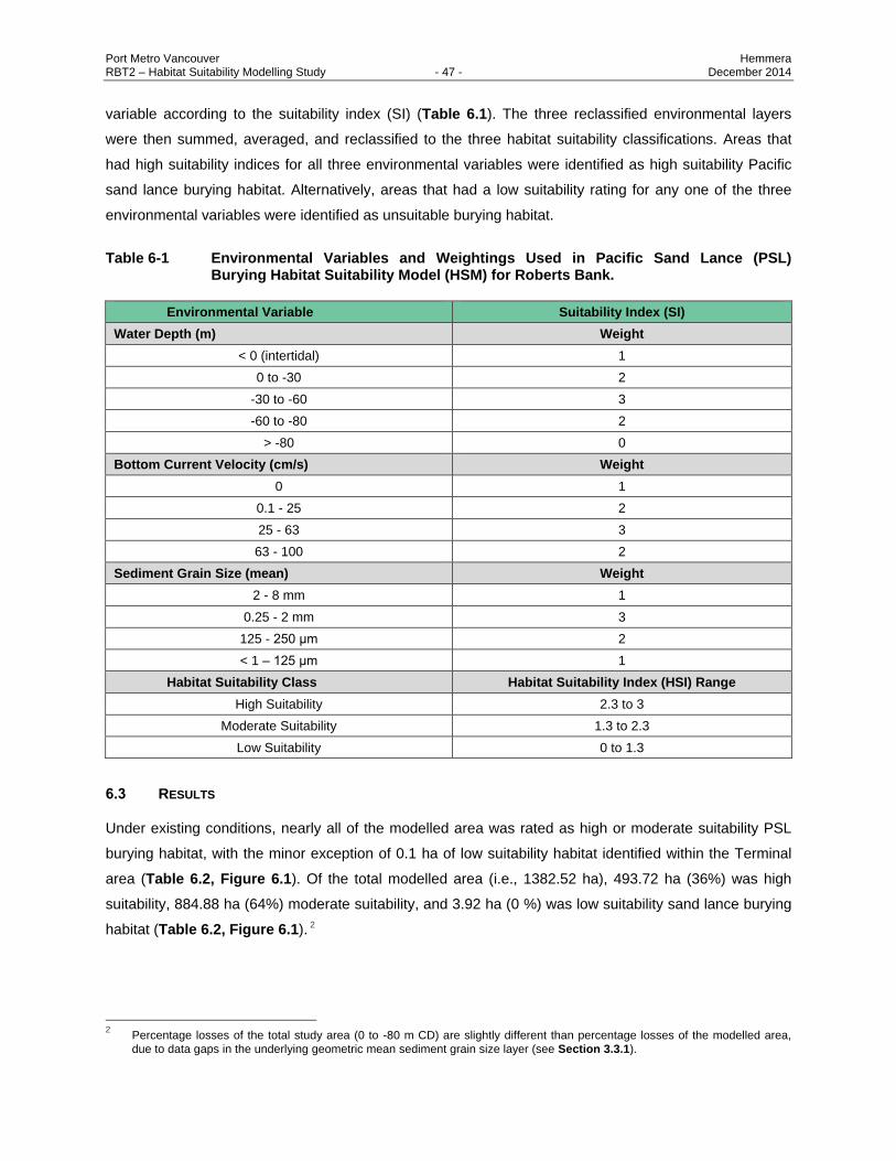
Port Metro Vancouver Hemmera RBT2 – Habitat Suitability Modelling Study - 47 - December 2014
variable according to the suitability index (SI) (Table 6.1). The three reclassified environmental layers
were then summed, averaged, and reclassified to the three habitat suitability classifications. Areas that
had high suitability indices for all three environmental variables were identified as high suitability Pacific
sand lance burying habitat. Alternatively, areas that had a low suitability rating for any one of the three
environmental variables were identified as unsuitable burying habitat.
Table 6-1 Environmental Variables and Weightings Used in Pacific Sand Lance (PSL) Burying Habitat Suitability Model (HSM) for Roberts Bank.
Environmental Variable Suitability Index (SI)
Water Depth (m) Weight
< 0 (intertidal) 1
0 to -30 2
-30 to -60 3
-60 to -80 2
> -80 0
Bottom Current Velocity (cm/s) Weight
0 1
0.1 - 25 2
25 - 63 3
63 - 100 2
Sediment Grain Size (mean) Weight
2 - 8 mm 1
0.25 - 2 mm 3
125 - 250 μm 2
< 1 – 125 μm 1
Habitat Suitability Class Habitat Suitability Index (HSI) Range
High Suitability 2.3 to 3
Moderate Suitability 1.3 to 2.3
Low Suitability 0 to 1.3
6.3 RESULTS
Under existing conditions, nearly all of the modelled area was rated as high or moderate suitability PSL
burying habitat, with the minor exception of 0.1 ha of low suitability habitat identified within the Terminal
area (Table 6.2, Figure 6.1). Of the total modelled area (i.e., 1382.52 ha), 493.72 ha (36%) was high
suitability, 884.88 ha (64%) moderate suitability, and 3.92 ha (0 %) was low suitability sand lance burying
habitat (Table 6.2, Figure 6.1). 2
2 Percentage losses of the total study area (0 to -80 m CD) are slightly different than percentage losses of the modelled area,
due to data gaps in the underlying geometric mean sediment grain size layer (see Section 3.3.1).
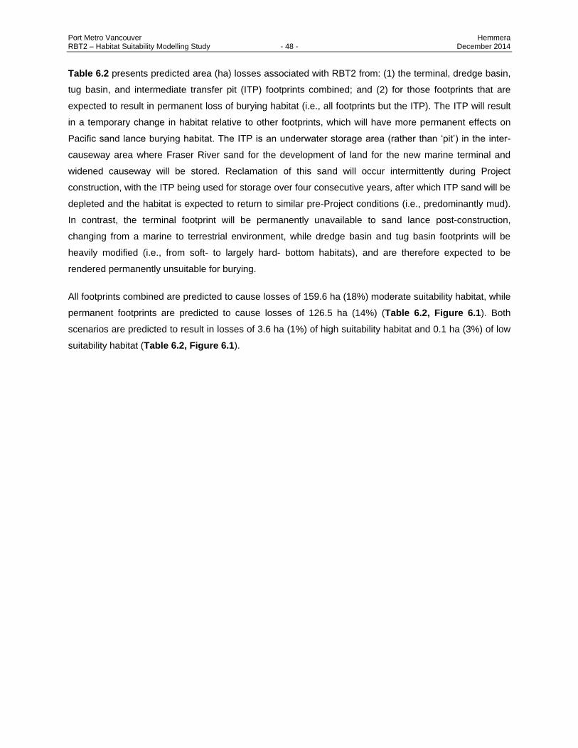
Port Metro Vancouver Hemmera RBT2 – Habitat Suitability Modelling Study - 48 - December 2014
Table 6.2 presents predicted area (ha) losses associated with RBT2 from: (1) the terminal, dredge basin,
tug basin, and intermediate transfer pit (ITP) footprints combined; and (2) for those footprints that are
expected to result in permanent loss of burying habitat (i.e., all footprints but the ITP). The ITP will result
in a temporary change in habitat relative to other footprints, which will have more permanent effects on
Pacific sand lance burying habitat. The ITP is an underwater storage area (rather than ‘pit’) in the inter-
causeway area where Fraser River sand for the development of land for the new marine terminal and
widened causeway will be stored. Reclamation of this sand will occur intermittently during Project
construction, with the ITP being used for storage over four consecutive years, after which ITP sand will be
depleted and the habitat is expected to return to similar pre-Project conditions (i.e., predominantly mud).
In contrast, the terminal footprint will be permanently unavailable to sand lance post-construction,
changing from a marine to terrestrial environment, while dredge basin and tug basin footprints will be
heavily modified (i.e., from soft- to largely hard- bottom habitats), and are therefore expected to be
rendered permanently unsuitable for burying.
All footprints combined are predicted to cause losses of 159.6 ha (18%) moderate suitability habitat, while
permanent footprints are predicted to cause losses of 126.5 ha (14%) (Table 6.2, Figure 6.1). Both
scenarios are predicted to result in losses of 3.6 ha (1%) of high suitability habitat and 0.1 ha (3%) of low
suitability habitat (Table 6.2, Figure 6.1).

Port Metro Vancouver Hemmera RBT2 – Habitat Suitability Modelling Study - 49 - December 2014
Table 6-2 Areas (ha) of High, Moderate, and Low Suitability Subtidal Burying Habitat for Pacific Sand Lance (Ammodytes hexapterus) Without and With RBT2. Habitat Losses are Based on Direct Footprint Losses, and Do Not Include Indirect Effects from Changes in Coastal Geomorphology.
Habitat Suitability Category
Without RBT2 (Existing Conditions) With RBT2
Total Area (ha)
Modelled Area (%)
Percent of Study Area (0 to -80 m
CD)
Area Loss (ha)
Total Area Remaining
(ha)
Percent Lost (%)
Area Loss (ha)
(Permanent Loss Only)
Total Area Remaining
(ha)
Percent Lost (%)
High 493.7 36 34 3.6 490.1 1 3.6 490.1 1
Moderate 884.9 64 62 159.6 725.3 18 126.5 758.4 14
Low 3.9 0 0 0.1 3.8 3 0.1 3.8 3
Suitable (Mod. + High) 1378.6 100 96 163.2 1215.4 12 130.2 1248.4 9
Total 1382.5 100 96 163.3 1219.2 12 130.3 1252.3 9
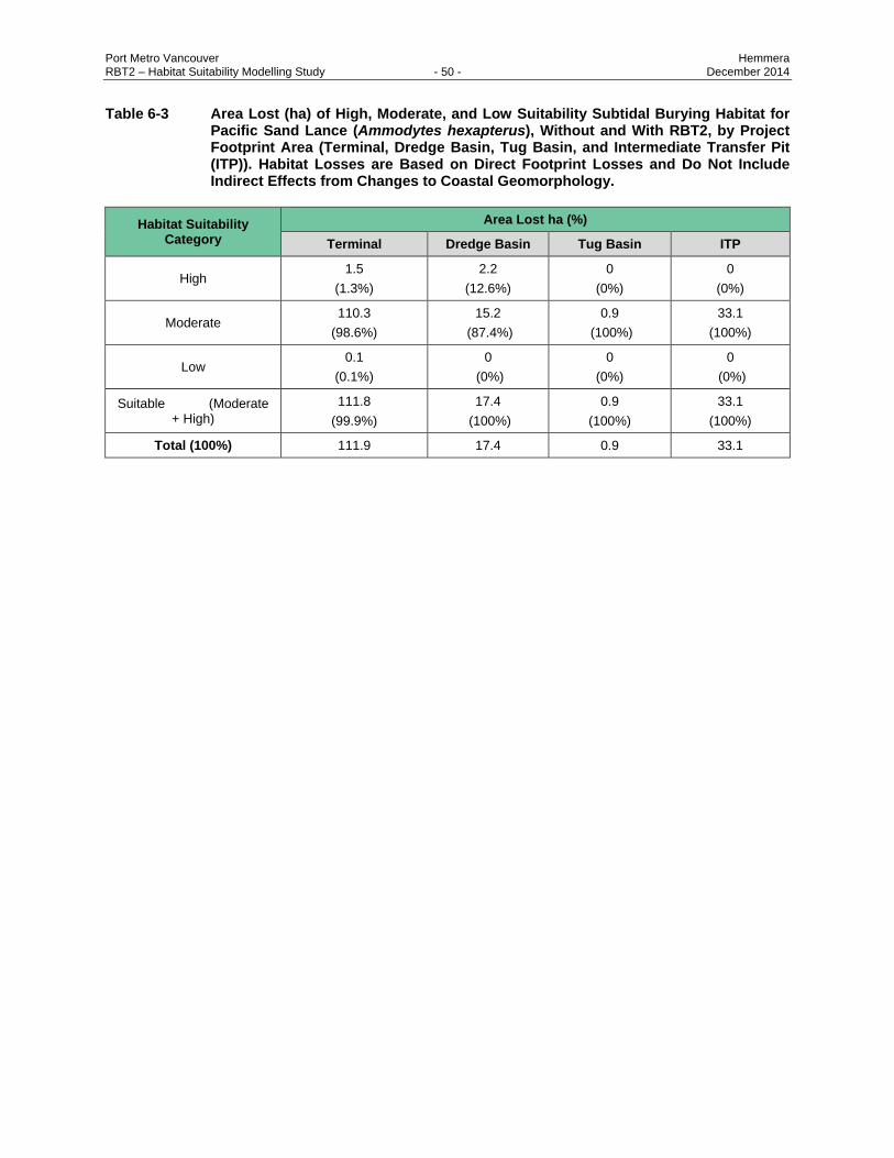
Port Metro Vancouver Hemmera RBT2 – Habitat Suitability Modelling Study - 50 - December 2014
Table 6-3 Area Lost (ha) of High, Moderate, and Low Suitability Subtidal Burying Habitat for Pacific Sand Lance (Ammodytes hexapterus), Without and With RBT2, by Project Footprint Area (Terminal, Dredge Basin, Tug Basin, and Intermediate Transfer Pit (ITP)). Habitat Losses are Based on Direct Footprint Losses and Do Not Include Indirect Effects from Changes to Coastal Geomorphology.
Habitat Suitability Category
Area Lost ha (%)
Terminal Dredge Basin Tug Basin ITP
High 1.5
(1.3%)
2.2
(12.6%)
0
(0%)
0
(0%)
Moderate 110.3
(98.6%)
15.2
(87.4%)
0.9
(100%)
33.1
(100%)
Low 0.1
(0.1%)
0
(0%)
0
(0%)
0
(0%)
Suitable (Moderate + High)
111.8
(99.9%)
17.4
(100%)
0.9
(100%)
33.1
(100%)
Total (100%) 111.9 17.4 0.9 33.1
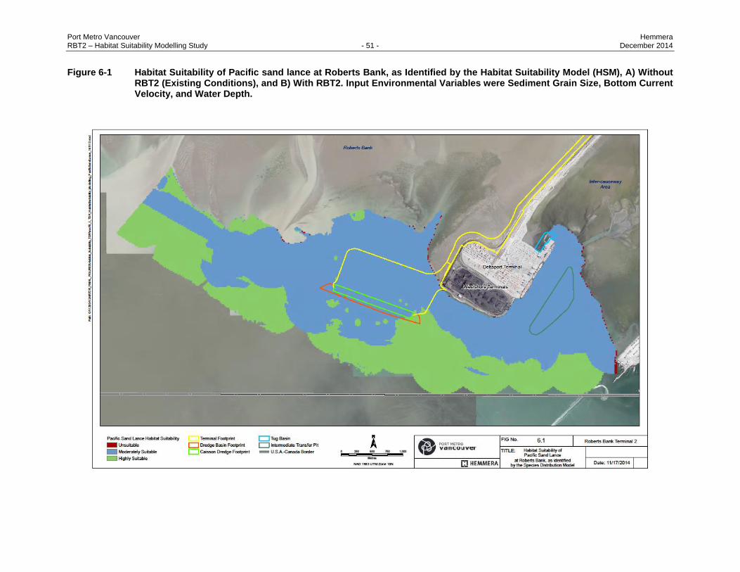
Port Metro Vancouver Hemmera RBT2 – Habitat Suitability Modelling Study - 51 - December 2014
Figure 6-1 Habitat Suitability of Pacific sand lance at Roberts Bank, as Identified by the Habitat Suitability Model (HSM), A) Without RBT2 (Existing Conditions), and B) With RBT2. Input Environmental Variables were Sediment Grain Size, Bottom Current Velocity, and Water Depth.
Port Metro Vancouver Hemmera RBT2 – Habitat Suitability Modelling Study - 52 - December 2014
6.4 DISCUSSION
The Pacific sand lance HSM suggests that of the approximately 500 ha of high suitability burying habitat
modelled, approximately 1% (3.6 ha) will be directly and permanently lost due to terminal, dredge basin,
and tug basin footprints. Of the moderate suitability habitat (i.e., ~880 ha), approximately 18% (159.2 ha)
will be permanently lost. Within the modelled area, there are small amounts of low suitability habitat
(i.e., ~3.9 ha) and only small amounts of change are anticipated to this habitat (i.e., ~1% or 0.1 ha of
permanent loss from Project footprints) (Table 6.2, Figure 6.1). Overall, these permanent losses of high
and moderate suitability burying habitat from Project footprints are not likely to substantially affect burying
habitat availability for Pacific sand lance at Roberts Bank (i.e., predicted area losses of moderate and
high suitability habitat considered together represent only 12% of the modelled suitable burying habitat)
(Table 6.2, Figure 6.1).
Habitat losses at the ITP (i.e., ~ 33 ha) due to sand dumping and intermittent disturbance from Project-
related reclamation (i.e., dredging, etc.) are expected to occur during construction, but will be temporary
and limited to moderate suitability habitat. All of the high suitability habitat losses will occur at the terminal
and dredge basin.
Numerous studies have examined the relationship between Ammodytes spp. burying and environmental
characteristics in laboratories (Winslade 1974, Pinto et al. 1984) and in the field in subtidal areas (Wright
et al. 2000, Holland et al. 2005, Ostrand et al. 2005, Haynes et al. 2007). However, Pacific sand lance
use of intertidal environments for burying is not well understood, even though the intertidal zone is
thought to be important habitat for this species (Robards and Piatt 1999, Haynes et al. 2008). Pacific
sand lance have been observed burying in the intertidal zone above the waterline as the tide recedes
(Quinn 1999, Haynes 2006); however, the characteristics of intertidal sediment that supports burying
have not been directly quantified in the field (Haynes et al. 2008). Haynes et al. (2008) modelled
nearshore intertidal habitat use of young-of-the-year (YOY), and while the focus of their study was not on
burying habitat (i.e., they sampled using a beach seine) their results suggest that intertidal sediment types
used may differ from those used in subtidal regions. The authors suggest that burying in intertidal
environments (especially above the waterline) may present Pacific sand lance with physiological
constraints beyond those faced in the subtidal, resulting in different sediment requirements or preferences
between the two zones (Haynes et al. 2008).
While the Haynes et al. (2008) study begins to identify intertidal habitat features that are important to
Pacific sand lance, specific burying preferences from intertidal field data are still lacking, precluding a
habitat suitability assessment of intertidal burying at Roberts Bank. Additionally, results from Haynes et al.
(2008) indicate that extrapolation of known subtidal burying preferences to the intertidal is likely to result
in erroneous modelling results. However, one might assume that there are areas of the intertidal zone at
Roberts Bank that are suitable to sand lance burying. While we are unable to model the size of these

Port Metro Vancouver Hemmera RBT2 – Habitat Suitability Modelling Study - 53 - December 2014
areas (or provide suitability classifications), the loss of suitable burying habitat presented herein from
terminal footprints in the subtidal likely represents a smaller percentage of the overall suitable burying
habitat available at Roberts Bank, if both zones are considered.
There are a number of model limitations and key assumptions that need to be taken into consideration
when assessing or interpreting the model results presented here. Firstly, key assumptions underlying
HSMs are that observed responses of target species to environmental characteristics are repeated
(and expected); and that environmental characteristics chosen as base layers are the key drivers of
suitability. While the variables chosen for the Pacific sand lance burying model presented here are similar
to those used in previous HSMs for this species (e.g., Robinson et al. 2013), there are other variables that
may be affecting sand lance burying at Roberts Bank that were not included in the model. For example,
Ostrand et al. (2005) modelled habitat selection by Pacific sand lance by examining their distribution
relative to water depth, distance to shore, bottom slope, bottom type, distance from sand bottom, and
shoreline type, and found selection of shallow water by sand lance, with weaker association between
sand lance distribution and beach shorelines, sand bottoms, distance to shore, bottom slope, and
distance to the nearest sand bottom (Ostrand et al. 2005). While this study did not examine burying
habitat specifically, it does suggest that a complex suite of environmental variables may be affecting sand
lance burying beyond those included in the Roberts Bank subtidal burying HSM. However, detailed
information on environmental preferences for other variables was not available from the literature,
precluding an inclusion of these in the model presented here.
Using average-rating habitat suitability models, due to their inherent nature, make it difficult to refine
habitat suitability rankings beyond the “suitable” classification; in other words, the relative quality of the
habitat within “suitable” classifications remains unknown. This is dependent of the spatial scale of the
input data, the scale at which patterns of suitability exist, and the spatial scales at which Pacific sand
lance interact with environmental variables. These HSMs provide a coarse and broad scale estimate of
potential habitat availability, but are likely not sensitive to fine scale patterns of usage.
Another limitation of the Pacific sand lance HSM is the reliance on environmental variables and
preference ranges from published literature rather than site-specific data, resulting in a model that
identifies an areas optimal habitat, but may be too conservative an estimate of realised habitat availability
(Robinson et al. 2013). Habitats with values ranging widely outside of these optima are unlikely to be
suitable for Pacific sand lance burying; however, habitat with values only slightly outside of these optima
may support burying on occasion.

Port Metro Vancouver Hemmera RBT2 – Habitat Suitability Modelling Study - 54 - December 2014
7.0 GENERAL DISCUSSION
A discussion of the major results arising from the Habitat Suitability Modelling Study and data gaps are
provided below.
7.1 DISCUSSION OF KEY FINDINGS
The HSMs quantify areas of potentially suitable habitat for each of the three focal species under
existing conditions. The predictive maps generated for orange sea pens (Figure 4.11), Dungeness crabs
(Figure 5.1) and Pacific sand lance (Figure 6.1) enables a priori identification of direct impacts to
available suitable habitat for these species.
Predicted losses of 27% of high suitability Orange sea pen habitat in the LSA due to the terminal footprint
will be countered by a net increase of 3.4 ha of high suitability habitat as moderate suitability habitat is
enhanced in localised areas around the Terminal by accelerated water flow increasing food delivery to
sea pens (Hemmera 2014b). Substantial amounts of high and moderate suitability Dungeness crab
habitat will remain available to Dungeness crabs outside the Project footprint. Despite remaining habitat
availability, permanent displacement from highly suitable subtidal sand habitat is considered to have a
minor negative effect on Dungeness crab productivity. Pacific sand lance are predicted to permanently
lose a total of 126.5 ha of moderate suitability and 3.6 ha of high suitability burying habitat to terminal
placement, and dredge and tug basin creation; this area loss constitutes approximately 9% of available
modelled suitable subtidal burying habitat in the LSA. Taken together, the information the HSMs provide
allow us to plan for anticipated direct effects of the Project and to mitigate effects, where possible.
Although HSMs have been particularly useful for rapid assessments of study areas and guiding
management of habitats where species abundance data is not always available (Aarts et al. 2013), the
predictive accuracy of HSMs is highly dependent on both the habitat variables used in the model
(Lee and Suen 2014) and the variability of the data being analysed (Austin 2007). In natural
environments, species distributions are often driven by many environmental conditions or resources that
may be highly variable through space and time; thus, simple HSMs are often limited by the assumption
that habitat preferences are temporally and spatially static and fail to capture all of the variables effects
that govern species distributions (Hirzel and Le Lay 2008). Environmental variables that underlie habitat
selectivity and thus species distributions may also co-vary in a non-linearly manner (Ahmadi-Nedushan et
al. 2006). For example, simple HSMs generally ignore complex biological variables or trophic interactions
that can introduce variability into the model, and therefore add uncertainty to the relationship between
habitat suitability and the presence of a species (Austin 2007). More complex models are required to
incorporate ecological variables such as the presence of competitors, predators, or prey availability that
may otherwise be overlooked by simple abiotic habitat classifications (Hirzel and Le Lay 2008). In
addition, HSMs are poorly equipped to predict the influences of either positive or negative feedback

Port Metro Vancouver Hemmera RBT2 – Habitat Suitability Modelling Study - 55 - December 2014
dynamics (for example, aggregative behaviours). The HSMs presented here provide a useful first
approximation of habitat availability for three key species at Roberts Bank, and use the best available
information on these species (from the literature and targeted RBT2 field studies) to evaluate potential
habitat losses associated with the Project. A final important point is that habitat availability, as identified
through applications of HSMs or other approaches, is not synonymous with the realised presence or
productivity of a species. Rather, productivity and opportunity may be limited by other limiting factors,
such as the effects on sub-populations as a result of harvesting or predation, or based on longer term
temporal cycles and trends.
7.2 DATA GAPS AND LIMITATIONS
Site-specific data limitations add a measure of uncertainty to the habitat suitability models. Sediment
samples were collected at a scale that was logistically feasible but distances between individual data
points may mean interpolation of the data points are not scaled to sediment distribution patters across
Roberts Bank. In areas where sampling intensity was lower on average, there is greater uncertainty in the
interpolation between points. A lack of deeper water sampling meant that sediment maps were limited to
interpolate to existing sample points reducing the model extent. For example, in the Pacific sand lance
model a relatively small amount (~55 ha; 3 percent (%)) of the study domain (0 to -80 m CD; ~1,432 ha)
was not interpolated. Additionally, there was a lack of site-specific abundance data for sand lance to
inform environmental preference layers or verify model outputs. While observations from seine surveys
confirm the presence of Pacific sand lance within the subtidal zone at Roberts Bank (Archipelago 2014a),
very few have been caught or observed within sediment at Roberts Bank (Hemmera 2014a, d). This could
be due to inherent sampling difficulties associated with Pacific sand lances’ complex, alternating benthic-
pelagic life history, or due to a lack of burying.
The orange sea pen SDM was potentially limited by a decrease in sampling intensity farther from the
Project site. Habitat associations may be limited by not mapping the full correlation between occurrence
and environmental variable distributions. The scale at which organisms interact with their environment
and at which we have represented the habitat components (environmental variables) may not be
completely aligned. Both temporal and spatial scales, such as seasonal patterns or micro-habitat
requirements, may play important roles in determining habitat suitability. These finer resolution or
dynamic patterns were not included in any of the modeling efforts and classification of suitable habitat
needs to be assessed within the context of such scale mismatches.
The habitat suitability approaches included in this assessment can only provide estimates of what may be
optimal habitat. Realised habitat suitability through usage is a much more difficult question. In
environments with ample habitat availability, usage at any one area may be low in spite of suitability.
Validation of HSMs is often difficult to demonstrate and dependent on existing population levels, habitat
availability, and temporally dynamic movement of organisms. With greater amounts of location specific
Port Metro Vancouver Hemmera RBT2 – Habitat Suitability Modelling Study - 56 - December 2014
data, such as was used in the Orange sea pen species distribution model, allows for a test of model
validation. However, the validation is only appropriate for the region the data was collected and is not
suitable for the model to be applied to different regions.
Ultimately, habitat suitability models are tools that provide insight into potential areas that may be utilised
by the species in question. An understanding of areas of potential habitat availability can be used when
considering policy options that would affect habitat availability and provide a larger context to make
decisions against.

Port Metro Vancouver Hemmera RBT2 – Habitat Suitability Modelling Study - 57 - December 2014
8.0 CLOSURE
Major authors and reviewers of this Technical Report are listed below, along with their signatures.
Report prepared by: Hemmera Envirochem Inc.
Marina Winterbottom, MMM. Biologist
Scott Toews, MSc. Biologist
Romney McPhie, MSc. Biologist
Iva Popovic, MSc. Biologist
Laura White, PhD Marine Biologist and Technical Specialist Report peer reviewed by: Hemmera Envirochem Inc.
Doug Bright, PhD, R.P. Bio., P. Biol. Practice Leader - Environmental Risk Assessment
Port Metro Vancouver Hemmera RBT2 – Habitat Suitability Modelling Study - 58 - December 2014
9.0 REFERENCES
Aarts, G., J. Fieberg, S. Brasseur, and J. Matthiopoulos. 2013. Quantifying the effect of habitat availability
on species distributions. Journal of Animal Ecology 82:1135–1145.
Ahmadi-Nedushan, B., A. St-Hilaire, M. Bérubé, É. Robichaud, N. Thiémonge, and B. Bobée. 2006. A
review of statistical methods for the evaluation of aquatic habitat suitability for instream flow
assessment. River Research and Applications 22:503–523.
Archipelago. 2009. Section 10; Seapen Bed Interpretation; Section 11; Lingcod Egg Mass Survey. In:
Hemmera Envirochem Inc. 2009. T2 Environmental Baseline Monitoring Report. Prepared by
Archipelago Marine Research Ltd., Prepared for Hemmera Envirochem Inc.
Archipelago. 2011. CCIP Habitat Offsetting: Sea Pen Survey and Literature Review. Final, Prepared by
Archipelago Marine Research Ltd. for Hemmera Envirochem Inc.
Archipelago. 2014a. Archipelago Marine Research. 2014. Roberts Bank Terminal 2 technical data report:
Benthic fish trawl survey. Prepared for Hemmera, Vancouver, B.C. Available at:
http://www.robertsbankterminal2.com/
Archipelago. 2014b. Archipelago Marine Research. 2014. Roberts Bank Terminal 2 technical data report:
Eelgrass fish community survey. Prepared for Hemmera, Vancouver, B.C. Available at:
http://www.robertsbankterminal2.com/
Archipelago. 2014c. Archipelago Marine Research. 2014. Roberts Bank Terminal 2 technical data report:
Juvenile salmon surveys. Prepared for Hemmera, Vancouver, B.C. Available at:
http://www.robertsbankterminal2.com/
Archipelago. 2014d. Archipelago Marine Research. 2014. Roberts Bank Terminal 2 technical data report:
Forage fish beach spawn survey. Prepared for Hemmera, Vancouver, B.C. Available at:
http://www.robertsbankterminal2.com/
Armstrong, D. A., and D. R. Gunderson. 1985. The Role of Estuaries in Dungeness Crab Early Life
History: A Case Study in Grays Harbor, Washington. Pages 145–170 in. Alaska Sea Grant
Dungeness Crab Symposium Proceedings. Volume 85-3. Alaska Sea Grant.
Armstrong, D. A., C. Rooper, and D. Gunderson. 2003. Estuarine Production of Juvenile Dungeness
Crab, Cancer magister, and Contribution to the Oregon-Washington Coastal Fishery. Estuaries
26:1174–1188.
Armstrong, D., J. Armstrong, and P. Dinnel. 1988. Distribution, abundance and habitat associations of
Dungeness crab, Cancer magister, in Guemes Channel, San Juan Islands, Washington. Journal
of Shellfish Research 7:147–148.
Port Metro Vancouver Hemmera RBT2 – Habitat Suitability Modelling Study - 59 - December 2014
Ashley, G. M. (Symposium C. 1990. Classification of Large-Scale Subaqueous Bedforms: A New Look at
an Old Problem. Journal of Sedimentary Petrology 60:160 – 172.
Austin, M. P. 1998. An ecological perspective on biodiversity investigations: examples from Australian
eucalypt forests. Annals of the Missouri Botanical Garden 2–17.
Austin, M. 2007. Species distribution models and ecological theory: a critical assessment and some
possible new approaches. Ecological modelling 200:1–19.
Best, B. A. 1988. Passive suspension feeding in a sea pen: effects of ambient flow on volume flow rate
and filtering efficiency. The Biological Bulletin 175:332–342.
Birkeland, C. 1968. Reciprocal interactions between a single prey species, Ptilosarcus gurneyi, and its
complex of predators. M.Sc. Thesis, University of Washington.
Birkeland, C. 1969. Consequences of Differing Reproductive and Feeding Strategies for the Dynamics
and Structure of an Association Based on the Single Prey Species, Ptilosarcus gurneyi (Gray).
Ph.D. Thesis, University of Washington.
Birkeland, C. 1974. Interactions between a Sea Pen and Seven of Its Predators. Ecological Monographs
44:211–232.
Bunte, K., and S. R. Abt. 2001. Sampling surface and subsurface particle-size distributions in wadable
gravel-and cobble-bed streams for analyses in sediment transport, hydraulics, and streambed
monitoring. U.S. Department of Agriculture, Forest Service, Rocky Mountain Research Station,
Fort Collins, CO, USA.
Burd, B. J., P. A. G. Barnes, C. A. Wright, and R. E. Thomson. 2008a. A review of subtidal benthic
habitats and invertebrate biota of the Strait of Georgia, British Columbia. Marine Environmental
Research 66:S3–S38.
Burd, B. J., R. W. Macdonald, S. C. Johannessen, and A. van Roodselaar. 2008b. Responses of subtidal
benthos of the Strait of Georgia, British Columbia, Canada to ambient sediment conditions and
natural and anthropogenic depositions. Marine Environmental Research 66:S62–S79.
Burnham, K. P., and D. R. Anderson. 2002. Model selection and multimodel inference: A practical
information-theoretic approach. Second Edition. Springer-Verlag, Berlin.
Chia, F. S., and B. J. Crawford. 1973. Some observations on gametogenesis, larval development and
substratum selection of the sea pen Ptilosarcus gurneyi. Marine Biology 23:73–82.
Cianfrani, C., G. Le Lay, A. H. Hirzel, and A. Loy. 2010. Do habitat suitability models reliably predict the
recovery areas of threatened species? Journal of Applied Ecology 47:421–430.

Port Metro Vancouver Hemmera RBT2 – Habitat Suitability Modelling Study - 60 - December 2014
Cleaver. 1949. Preliminary results of the coastal crab (Cancer magister) investigation. Biological Report,
Washington State Department of Fisheries, Olympia, WA.
Community Mapping Network (CMN). 2013. Forage Fish Atlas and Data Management System.
Community Mapping Network. <http://www.cmnbc.ca/atlas_gallery/forage-fish-atlas-and-data-
management-system>.
Cohen, J. 1960. A coefficient of agreement for nominal l scales . Educational and Psychological
Measurement 20:37–46.
Conlin, K., B. Lawley, P. Futer, M. A. Abdelrhman, L. Jantz, B. Hillaby, R. Elvidge, B. Piercey, D. Gordon,
C. Levings, K. Hutton, and R. Maclndoe. 1982. Fraser estuary comparative habitat study: beach
seine catches, water characteristics and geomorphology March 1980 to July 1981. Canadian
Data Report of Fisheries and Aquatic Sciences, No. 340, Fisheries and Oceans Canada, West
Vancouver, B.C.
Curtis, D. L., and I. J. McGaw. 2012. Salinity and thermal preference of Dungeness crabs in the lab and in
the field: Effects of food availability and starvation. Journal of Experimental Marine Biology and
Ecology 413:113–120.
Curtis, D., and I. McGaw. 2008. A year in the life of a Dungeness crab: methodology for determining
microhabitat conditions experienced by large decapod crustaceans in estuaries. Journal of
Zoology 274:375–385.
Dethier, M. N. 2006. Native shellfish in nearshore ecosystems of Puget Sound. Puget Sound Nearshore
Partnership Report, Washington University Seattle Fisheries Research Institution, Seattle, WA.
<http://www.pugetsoundnearshore.org/technical_papers/shellfish.pdf>.
Van Deurs, M., A. Christensen, C. Frisk, and H. Mosegaard. 2010. Overwintering strategy of sandeel
ecotypes from an energy/predation trade-off perspective. Marine Ecology Progress Series
416:201–214.
Fisheries and Oceans Canada (DFO). 2011. Pacific Region Cold-Water Coral and Sponge Conservation
Strategy (2010-2015). Fisheries and Oceans Canada.
Dick, M. H., and I. M. Warner. 1982. Pacific sand lance Ammodytes hexapterus Pallas, in the Kodiak
Island group, Alaska. Syesis 15:43–50.
Dumbauld, B., and T. 1993. Use of oyster shell to enhance intertidal habitat and mitigate loss of
Dungeness Crab (Cancer magister) caused by dredging. Canadian Journal of Fisheries and
Aquatic Science 50:383–390.
Edwards, D., and C. Moore. 2008. Reproduction in the sea pen Pennatula phosphorea (Anthozoa:
Pennatulacea) from the west coast of Scotland. Marine Biology 155:303–314.

Port Metro Vancouver Hemmera RBT2 – Habitat Suitability Modelling Study - 61 - December 2014
ESRI. 2014. GIS Dictionary.
<http://support.esri.com/en/knowledgebase/GISDictionary/term/inverse%20distance%20weighted
%20interpolation>.
Fernandez, M., O. Iribarne, and D. A. Armstrong. 1993. Habitat selection by young-of-the-year
Dungeness crab, Cancer magister, and predation risk in intertidal habitats. Marine Ecology
Progress Series 92:171–177.
Field, L. J. 1988. Pacific sand lance, Ammodytes hexapterus, with notes on related Ammodytes species.
Species synopsis: life histories of selected fish and shellfish of the northeast Pacific and Bering
Sea 15–33.
Fuller, S. D., F. J. Murillo Perez, V. Wareham, and E. Kenchington. 2008. Vulnerable Marine Ecosystems
Dominated by Deep-Water Corals and Sponges in the NAFO Convention Area. Northwest
Atlantic Fisheries Organization.
Gartner Lee. 1992. Environmental appraisal of proposed terminal, Roberts Bank. Prepared by Gartner
Lee Ltd., Prepared for Vancouver Port Corporation, Burnaby, B.C.
Gotshall, D., and L. L. Laurent. 1979. Pacific Coast Subtidal Marine Invertebrates: A Fishwatcher’s Guide.
Sea Challengers.
De Graaf, R. C. 2007. Boundary Bay intertidal forage fish spawning habitat project: summery of project
and findings July 2006 – October 2007. Friends of Semiahmoo Bay Society Marine Conservation
Initiative.
Greenstreet, S. P., G. J. Holland, E. J. Guirey, E. Armstrong, H. M. Fraser, and I. M. Gibb. 2010.
Combining hydroacoustic seabed survey and grab sampling techniques to assess “local” sandeel
population abundance. ICES Journal of Marine Science 67:971–984.
Guisan, A., T. C. Edwards Jr, and T. Hastie. 2002. Generalized linear and generalized additive models in
studies of species distributions: setting the scene. Ecological modelling 157:89–100.
Guisan, A., R. Tingley, J. B. Baumgartner, I. Naujokaitis‐ Lewis, P. R. Sutcliffe, A. I. Tulloch, T. J. Regan,
L. Brotons, E. McDonald‐ Madden, and C. Mantyka‐ Pringle. 2013. Predicting species
distributions for conservation decisions. Ecology letters 16:1424–1435.
Gunderson, D. R., D. A. Armstrong, Y.-B. Shi, and R. A. McConnaughey. 1990. Patterns of estuarine use
by juvenile English sole (Parophrys vetulus) and Dungeness crab (Cancer magister). Estuaries
13:59–71.
Haynes, T. B., C. K. L. Robinson, and P. Dearden. 2008. Modelling nearshore intertidal habitat use of
young-of-the-year Pacific sand lance (Ammodytes hexapterus) in Barkley Sound, British
Columbia, Canada. Environmental Biology of Fishes 83:473–484.
Port Metro Vancouver Hemmera RBT2 – Habitat Suitability Modelling Study - 62 - December 2014
Haynes, T. B., R. A. Ronconi, and A. E. Burger. 2007. Habitat use and behavior of the Pacific sand lance
(Ammodytes hexapterus) in the shallow subtidal region of southwestern Vancouver Island.
Northwestern Naturalist 88:155–167.
Haynes, T. B. 2006. Modeling habitat use of young-of-the-year Pacific sand lance (Ammodytes
hexapterus) in the nearshore region of Barkley Sound, British Columbia. M.Sc. Thesis, University
of Victoria, Department of Geography, Victoria, B.C.
Healy, M. C. 1984. Laboratory spawning of Ammodytes hexapterus from the Pacific coast of North
America with a description of its eggs and early larvae. Copeia 1:242–244.
Hemmera and Archipelago. 2014. Roberts Bank Terminal 2 technical data report: Orange sea pens
(Ptilosarcus gurneyi). Prepared for Port Metro Vancouver, Vancouver, B.C. Available at:
http://www.robertsbankterminal2.com/
Hemmera. 2014a. Roberts Bank Terminal 2 technical data report: Sediment and water quality
characterisation studies. Prepared for Port Metro Vancouver, Vancouver, B.C. in Port Metro
Vancouver (PMV). 2015. Roberts Bank Terminal 2 Environmental impact statement: Volume 2.
Environmental Assessment by Review Panel. Submitted to Canadian Environmental Assessment
Agency.
Hemmera. 2014b. Roberts Bank Terminal 2 technical report: Habitat suitability modelling study. Prepared
for Port Metro Vancouver, Vancouver, B.C. in Port Metro Vancouver (PMV). 2015. Roberts Bank
Terminal 2 Environmental impact statement: Volume 3. Environmental Assessment by Review
Panel. Submitted to Canadian Environmental Assessment Agency.
Hemmera. 2014c. Roberts Bank Terminal 2 technical data report: Juvenile Dungeness crabs. Prepared
for Port Metro Vancouver, Vancouver, B.C. Available at: http://www.robertsbankterminal2.com/
Hemmera. 2014d. Roberts Bank Terminal 2 technical data report: Subtidal benthic infauna and epifauna
surveys for disposal at sea site characterisation. Prepared for Port Metro Vancouver, Vancouver,
B.C. Available at: http://www.robertsbankterminal2.com/
Hirzel, A., and A. Guisan. 2002. Which is the optimal sampling strategy for habitat suitability modelling.
Ecological modelling 157:331–341.
Hirzel, A. H., and G. Le Lay. 2008. Habitat suitability modelling and niche theory. Journal of Applied
Ecology 45:1372–1381.
Hobson, E. S. 1986. Predation on the Pacific sand lance, Ammodytes hexapterus (Pisces:
Ammodytidae), during the transition between day and night in southeastern Alaska. Copeia
1986:223–226.
Port Metro Vancouver Hemmera RBT2 – Habitat Suitability Modelling Study - 63 - December 2014
Holland, G. J., S. P. R. Greenstreet, I. M. Gibb, H. M. Fraser, and M. R. Robertson. 2005. Identifying
sandeel Ammodytes mainus sediment habitat preferences in the marine environment. Marine
Ecology Progress Series 303:269 – 282.
Holsman, K. K., D. A. Armstrong, D. A. Beauchamp, and J. L. Ruesink. 2003. The necessity for intertidal
foraging by estuarine populations of subadult Dungeness crab, Cancer magister: evidence from a
bioenergetics model. Estuaries 26:1155–1173.
Holsman, K. K., P. S. McDonald, and D. A. Armstrong. 2006. Intertidal migration and habitat use by
subadult Dungeness crab Cancer magister in a NE Pacific estuary. Marine Ecology Progress
Series 308:183–195.
Hosmer, D. W., and S. Lemeshow. 2004. Applied logistic regression. John Wiley & Sons.
Jenness, J. 2006. Topographic Position Index (tpi_jen. avx) extension for ArcView 3. x, v. 1.3 a. Jenness
Enterprises.
Johnson, S. W., J. F. Thedinga, A. D. Neff, R. A. Heintz, M. R. Lindeberg, P. M. Harris, and S. D. Rice.
2008. Seasonal distribution, habitat use, and energy density of forage fish in the nearshore
ecosystem of Prince William Sound, Alaska. North Pacific Research Board Project 642, Final
Report, National Oceanic and Atmospheric Administration, National Marine Fisheries Service,
Juneau, AK.
Van der Kooij, J., B. E. Scott, and S. Mackinson. 2008. The effects of environmental factors on daytime
sandeel distribution and abundance on the Dogger Bank. Journal of Sea Research 60:201–209.
Kühlmann, D. H., and H. Karst. 1967. Freiwasserbeobachtungen zum Verhalten von
Tobiasfischschwärmen (Ammodytidae) in der westlichen Ostsee*. Zeitschrift für Tierpsychologie
24:282–297.
Kyte, M. A. 2001. Vacant Benthic Habitats: Where Have All the Sea Pens Gone? Pacific Estuarine
Research Society.
Lamb, A., and B. P. Hanby. 2005. Marine life of the Pacific Northwest: a photographic encyclopedia of
invertbrates, seaweeds and selected fishes. Harbour Publishing, Madeira Park, CB.
Latif, Q. S., V. A. Saab, J. G. Dudley, and J. P. Hollenbeck. 2013. Ensemble modeling to predict habitat
suitability for a large-scale disturbance specialist. Ecology and Evolution 3:4348–4364.
Lee, P.-Y., and J.-P. Suen. 2014. Dependency and independency among fish density and electivity
indices in a stream fish assemblage. Environmental Biology of Fishes 97:111–119.
Macer, C. 1966. Sand eels (Ammodytidae) in the south-western North Sea; their biology and fishery.

Port Metro Vancouver Hemmera RBT2 – Habitat Suitability Modelling Study - 64 - December 2014
Martel, G. 2009. T2 Environmental Baseline Monitoring Report, Section 9: Juvenile Dungeness Crabs.
Prepared for Vancouver Port Authority, Vancouver, BC.
Mayer, D. L. 1979. The ecology and thermal sensitivity of the Dungeness crab, Cancer magister, and
related species of its benthic community in Similk Bay, Washington. Ph.D. Thesis, University of
Washington.
McGaw, I. J. 2005. Burying behaviour of two sympatric crab species: Cancer magister and Cancer
productus. Scientia Marina 69:375–381.
McMillan, R. O., D. A. Armstrong, and P. A. Dinnel. 1995. Comparison of intertidal habitat use and growth
rates of two northern Puget Sound cohorts of 0+ age Dungeness crab, Cancer magister.
Estuaries 18:390–398.
Meyer, T. L., R. A. Cooper, and R. W. Langton. 1979. Relative abundance, behavior, and food habits of
the American sand lance, Ammodytes americanus, from the Gulf of Maine. Fishery Bulletin
77:243–253.
Minns, C. K., R. G. Randall, K. E. Smokorowski, K. D. Clarke, A. Vélez-Espino, R. S. Gregory, S.
Courtenay, and P. LeBlanc. 2011. Direct and indirect estimates of the productive capacity of fish
habitat under Canada’s Policy for the Management of Fish Habitat: where have we been, where
are we now, and where are we going? Canadian Journal of Fisheries and Aquatic Sciences
68:2204–2227.
Murase, H., H. Nagashima, S. Yonezaki, R. Matsukura, and T. Kitakado. 2009. Application of a
generalized additive model (GAM) to reveal relationships between environmental factors and
distributions of pelagic fish and krill: a case study in Sendai Bay, Japan. ICES Journal of Marine
Science 66:1417–1424.
Northwest Hydraulic Consultants (NHC). 2014. Roberts Bank Terminal 2 technical report: Coastal
geomorphology study. Prepared for Port Metro Vancouver, Vancouver, B.C. in Port Metro
Vancouver (PMV). 2015. Roberts Bank Terminal 2 Environmental impact statement: Volume 2.
Environmental Assessment by Review Panel. Submitted to Canadian Environmental Assessment
Agency.
O’Clair, C. E., T. C. Shirley, and S. J. Taggart. 1996. Dispersion of adult Cancer magister at Glacier Bay,
Alaska: Variation with spatial scale, sex, and reproductive status. Pages 209–227 in. High latitude
crabs: Biology, management, and economics. University of Alaska Sea Grant, AK-SG-96-02,
Fairbanks, Alaska.
O’Connell, M., and J. M. Fives. 1995. the biology of the lesser sand-eel Ammodytes tobianus L. in the
Galway Bay area. Pages 87–98 in. Biology and Environment: Proceedings of the Royal Irish
Academy. JSTOR. <http://www.jstor.org.proxy.lib.sfu.ca/stable/20504502>. Accessed 10 Dec
2014.

Port Metro Vancouver Hemmera RBT2 – Habitat Suitability Modelling Study - 65 - December 2014
Ostrand, W. D., T. A. Gotthardt, S. Howlin, and M. D. Robards. 2005. Habitat selection models for Pacific
sand lance (Ammodytes hexapterus) in Prince William Sound, Alaska. Northwest Naturalist
86:131–143.
Pauley, G. B., D. A. Armstrong, R. Van Citter, and G. Thomas. 1989. Species profiles: life histories and
environmental requirements of coastal fishes and invertebrates (Pacific Southwest), Dungeness
crab.
Pearson, W. H., D. L. Woodruff, P. C. Sugarman, and B. L. Olla. 1984. The burrowing behavior of sand
lance, Ammodytes hexapterus: Effects of oil-contaminated sediment. Marine Environmental
Research 11:17–32.
Penttila, D. E. 1995. Investigations of the spawning habitat of the Pacific sand lance, Ammodytes
hexapteru. Pages 855–859 in. Puget Sound Research-95 Conference Proceedings. Volume 2.
Puget Sound Water Authority, Olympia, WA.
Penttila, D. E. 1999. Documented spawning areas of the Pacific herring (Clupea), surf smelt
(Hypomesus), and Pacific sand lance (Ammodytes) in San Juan County, Washington.
Washington Department of Fish and Wildlife, Marine Resources Division, Washington, U.S.A.
Penttila, D. 2000. Grain size analysis of spawning substrates of the surf smelt (Hypomesus) and Pacific
sand lance (Ammodytes) on Puget Sound spawning beaches. Data Summary, State of
Washington Department of Fish and Wildlife, Marine Resources Division, La Conner, WA.
Penttila, D. 2007. Marine forage fishes in Puget Sound. Technical Report 2007-03, Washington
Department of Fish and Wildlife.
Pinto, J. M., W. H. Pearson, and J. W. Anderson. 1984. Sediment preferences and oil contamination in
the Pacific sand lance Ammodytes hexapterus. Marine Biology 83:193–204.
Posada, D., and T. R. Buckley. 2004. Model selection and model averaging in phylogenetics: advantages
of Akaike information criterion and Bayesian approaches over likelihood ratio tests. Systematic
biology 53:793–808.
Quinn, T. 1987. Physiological ecology of Ammodytes hexapterus in relation to its burrowing behavior.
M.Sc. Thesis, Western Washington University, Bellingham, WA.
Quinn, T. 1999. Habitat characteristics of an intertidal aggregation of Pacific sand lance (Ammodytes
hexapterus) at a North Puget Sound beach in Washington. Northwest Science 73:44–49.
R Development Core Team. 2014. R: a language and environment for statistical computing. R Foundation
for Statistical Computing, Vienna, Austria. <http://www.R-project.org/>.
Port Metro Vancouver Hemmera RBT2 – Habitat Suitability Modelling Study - 66 - December 2014
Rasmuson, L. K. 2013. The Biology, Ecology and Fishery of the Dungeness Crab, Cancer magister.
Advances in Marine Biology 65:95–148.
Reay, P. 1970. Synopsis of biological data on North Atlantic sandeels of the genus Ammodytes (A.
tobianus, A. dubius, A. americanus and A. marinus). Food and Agriculture Organization of the
United Nations.
Robards, M. D., and J. F. Piatt. 1999. Biology of the genus Ammodytes, the sand lances. USDA Forest
Service Pacific Northwest Research Station Research Paper 1–16.
Robards, M. D., G. A. Rose, and J. F. Piatt. 2002. Growth and abundance of Pacific sand lance,
Ammodytes hexapterus, under differing oceanographic regimes. Environmental Biology of Fishes
64:429–441.
Robards, M. D., M. F. Willson, R. H. Armstrong, and J. F. Piatt. 1999. Sand lance: a review of biology and
predator relations and annotated bibliography. Exxon Valdez Oil Spill Restoration Project, PNW-
RP 521, U.S. Department of Agriculture, Forest Service, Pacific Northwest Research Station,
Portland, OR.
Robinson, C. L., J. Yakimishyn, and M.-J. Rochet. 2013. The persistence and stability of fish
assemblages within eelgrass meadows (Zostera marina) on the Pacific coast of Canada.
Canadian Journal of Fisheries and Aquatic Sciences 70:775–784.
Robinson, C. L., and J. Yakimishyn. 2013. The persistence and stability of fish assemblages within
eelgrass meadows (Zostera marina) on the Pacific coast of Canada. Canadian Journal of
Fisheries and Aquatic Sciences 70:775–784.
Rooper, C. N., D. A. Armstrong, and D. R. Gunderson. 2002. Habitat use by Juvenile Dungeness Crabs
in Coastal Nursery Estuaries. Crabs in Cold Water Regions: Biology, Management, and
Economics Alaska Sea Grant College Program.
Rotenberry, J. T., K. L. Preston, and S. T. Knick. 2006. GIS-BASED NICHE MODELING FOR MAPPING
SPECIES’HABITAT. Ecology 87:1458–1464.
Scheding, K., T. Shirley, C. E. O’Clair, and S. J. Taggart. 2001. Critical habitat for ovigerous Dungeness
crabs. Pages 431–445 in G. H. Kruse, B. Nicolas, A. Booth, M. W. Dorn, S. Hills, R. N. Lipcius, D.
Pelletier, C. Roy, S. J. Smith, and D. Witherell, editors. Spatial Processes and Management of
Marine Populations. University of Alaska Sea Grant, AK-SG-01-02, Fairbanks, Alaska.
<http://nsgl.gso.uri.edu/aku/akuw99004/akuw99004_full.pdf#page=441>. Accessed 14 Jan 2014.
Shepherd, D. A. 1988. Foraging interactions among Black-billed Magpies, Northwestern Crows, and Red
Foxes on Kodiak Island, Alaska. Society for Northwestern Vertebrate Biology.
Shimek, R. L. 2011. The life and death of sea pens. Reefkeeping Magazine 1–19.

Port Metro Vancouver Hemmera RBT2 – Habitat Suitability Modelling Study - 67 - December 2014
Shirley, S. M., T. C. Shirley, and S. D. Rice. 1987. Latitudinal variation in the Dungeness crab, Cancer
magister: zoeal morphology explained by incubation temperature. Marine Biology 95:371–376.
Stevens, B. G., and D. A. Armstrong. 1985. Ecology, growth and population dynamics of juvenile
Dungeness crab, Cancer magister Dana, in Grays Harbor, Washington. Pages 119–134 in.
Symposium on Dungeness crab biology and management.
Stone, R. P., and C. E. O’Clair. 2002. Behavior of female Dungeness crabs, Cancer magister, in a glacial
southeast Alaska estuary: homing, brooding-site fidelity, seasonal movements, and habitat use.
Journal of Crustacean Biology 22:481–492.
Stoner, A. W., M. L. Spencer, and C. H. Ryer. 2007. Flatfish-Habitat Associations in Alaska Nursery
Grounds: Use of Continuous Video Records for Multi-Scale Spatial Analysis. Journal of Sea
Research 57:137 – 150.
Tasto, R. N. 1983. Juvenile Dungeness Crab, Cancer magister, Studies in the San Francisco Bay Area.
Pages 135–154 in P. W. Wild and R. N. Tasto, editors. Life History, Environment, and Mariculture
Studies of the Dungeness Crab. Cancer magister, with Emphasis on the Central California
Fishery Resource. Volume 172. Fishery Bulletin, California Department of Fish and Game.
Therriault, T. W., D. E. Hay, and J. F. Schweigert. 2009. Biological overview and trends in pelagic forage
fish abundance in the Salish Sea (Strait of Georgia, British Columbia). Marine Ornithology 37:3–
8.
Thomson, R. . 1981. Oceanography of the British Columbia coast. Volume Vol. 56. Department of
Fisheries and Oceans, Sidney, B.C.
Thuringer, P. L. 2004. Documenting Pacific sand lance (Ammodytes hexapterus) spawning habitat in
Baynes Sound, east coast Vancouver Island, and the potential interactions with intertidal shellfish
aquaculture. M.Sc. Thesis, Royal Roads University, Victoria, B.C.
Thuringer, P. 2003. Documenting Pacific Sand Lance (Ammodtyes hexapterus) Spawning Habitat in
Baynes Sound and the Potential Interactions with Intertidal Shellfish Aquaculture. Draft Final
Report, Archipelago Marine Research Ltd., Victoria, B.C.
Tissot, B. N., M. S. Love, K. York, and M. Amend. 2006. Benthic invertebrates that form habitat on deep
banks off southern California, with special reference to deep sea coral. Fishery Bulletin 104:167–
181.
Tokranov, A. M. 2007. Distribution and Some Biological Features of the Pacific Sand Lance Ammodytes
hexapterus (Ammodytidae) in Waters off Kamchatka in the Sea of Okhotsk. Journal of Icthyology
47:288 – 295.

Port Metro Vancouver Hemmera RBT2 – Habitat Suitability Modelling Study - 68 - December 2014
Triton. 2004. Deltaport Third Berth Project Marine Resources Impact Assessment. Prepared by Triton
Environmental Consultants Ltd., Prepared for Vancouver Port Authority, Richmond, B.C.
Vavrinec, J., W. H. Pearson, N. P. Kohn, J. R. Skalski, C. Lee, K. D. Hall, B. A. Romano, M. C. Miller, and
T. P. Khangaonkar. 2007. Laboratory Assessment of Potential Impacts to Dungeness Crabs from
Disposal of Dredged Material from the Columbia River. Pacific Northwest National Laboratory.
Weightman, J. O., and D. J. Arsenault. 2002. Predator classification by the sea pen Ptilosarcus gurneyi (
Cnidaria ): role of waterborne chemical cues and physical contact with predatory sea stars.
Canadian journal of zoology 80:185–190.
Wild, P. W. 1980. Effects of seawater temperature on spawning, egg development, hatching success, and
population fluctuations of the Dungeness crab, Cancer magister. CalCOFI Reports XXI.
Willson, M. F., R. H. Armstrong, M. D. Robards, and J. F. Piatt. 1999. Sand lance as cornerstone prey for
predator populations. M. D. Robards, M. F. Willson, R. H. Armstrong, and J. F. Piatt, editors.
Sand lance: a review of biology and predator relations and annotated bibliography. Research
Paper PNW-RP-521, U.S. Forest Service.
Winslade, P. 1974. Behavioural studies on the lesser sandeel Ammodytes marinus (Raitt) I. The effect of
food availability on activity and the role of olfaction in food detection. Journal of Fish Biology
6:565–576.
Wright, D., M. Pendleton, J. Boulware, S. Walbridge, B. Gerlt, D. Eslinger, D. Sampson, and E. Huntley.
2012. ArcGIS Benthic Terrain Modeler (BTM), v. 3.0, Environmental Systems Research Institute,
NOAA Coastal Services Center, Massachusetts Office of Coastal Zone Management.
Wright, P. J., H. Jensen, and I. Tuck. 2000. The influence of sediment type on the distribution of the
lesser sandeel,Ammodytes marinus. Journal of Sea Research 44:243–256.
Wright, P. J., S. A. Pederson, L. Donald, C. Anderson, P. Lewy, and R. Proctor. 1998. The influence of
physical factors on the distribution of lesser sandeels and its relevance to fishing pressure in the
North Sea. ICES Council Meeting Paper 1998/AA. Volume 3.
Zhang, Z., W. Hajas, A. Phillips, and J. A. Boutillier. 2004. Use of length-based models to estimate
biological parameters and conduct yield analyses for male Dungeness crab (Cancer magister).
Canadian Journal of Fisheries and Aquatic Sciences 61:2126–2134.
Port Metro Vancouver Hemmera RBT2 – Habitat Suitability Modelling Study - 69 - December 2014
10.0 STATEMENT OF LIMITATIONS
This report was prepared by Hemmera Envirochem Inc.(Hemmera), based on fieldwork and modelling
conducted by Hemmera for the sole benefit and exclusive use of Port Metro Vancouver. The material in it
reflects Hemmera’s best judgment in light of the information available to it at the time of preparing this
Report. Any use that a third party makes of this Report, or any reliance on or decision made based on it,
is the responsibility of such third parties. Hemmera accept no responsibility for damages, if any, suffered
by any third party as a result of decisions made or actions taken based on this Report.
Hemmera has performed the work as described above and made the findings and conclusions set out in
this Report in a manner consistent with the level of care and skill normally exercised by members of the
environmental science profession practicing under similar conditions at the time the work was performed.
This Report represents a reasonable review of the information available to NHC and Hemmera within the
established Scope, work schedule and budgetary constraints. The conclusions and recommendations
contained in this Report are based upon applicable legislation existing at the time the Report was drafted.
Any changes in the legislation may alter the conclusions and/or recommendations contained in the
Report. Regulatory implications discussed in this Report were based on the applicable legislation existing
at the time this Report was written.
In preparing this Report, Hemmera has relied in good faith on information provided by others as noted in
this Report, and has assumed that the information provided by those individuals is both factual and
accurate. Hemmera accepts no responsibility for any deficiency, misstatement or inaccuracy in this
Report resulting from the information provided by those individuals.
APPENDIX A
Data Origins of Environmental Variables

Port Metro Vancouver APPENDIX A Hemmera RBT2 – Habitat Suitability Modelling Study - 1 - December 2014
Table A1 Data Origins of Environmental Variables Input to the Habitat Suitability Models (HSMs) for each Species Group.
Environmental Variables
Species Habitat Suitability Models
Orange sea pen
Dungeness crab Juveniles
Dungeness crab Adults
Dungeness crab Gravid Females
Pacific sand lance
Habitat Type N/A McMillian et al. 1995,
Pauly et al. 1986, Holsman et al. 2006
Pauly et al. 1986, Stone and O’Clair
2001, Dethier 2006.
Stone and O’Clair 2001
N/A
Sediment Grain Size
N/A Dethier 2006 Dethier 2006 Dethier 2006 Robinson
et al. 2013
Water Depth N/A Holsman et al. 2003, Holsman et al. 2006
Pauly et al. 1996, Fisher and
Velasquez 2008
Hemmera 2014, Fisher and
Velasquez 2008
Robinson et al. 2013
Salinity N/A Curtis and McGaw
2007 Curtis and McGaw
2007 Curtis and McGaw
2007 N/A
Slope Modeled Hemmera 2014 Hemmera 2014 Hemmera 2014 N/A
Bottom Current Velocity
Modeled N/A N/A N/A Robinson
et al. 2013
Wave Height Modeled N/A N/A N/A N/A
Fine Scale Bathymetric Position Index (BPI)
Modeled N/A N/A N/A N/A
Broad Scale BPI Modeled N/A N/A N/A N/A
APPENDIX B
Geospatial Interpolations –
Inverse Distance Weighting (IDW)
Port Metro Vancouver APPENDIX B Hemmera RBT2 – Habitat Suitability Modelling Study - 1 - December 2014
Background
Spatial interpolations, which help with spatial pattern analysis, were completed for the Habitat Suitability
Modelling TR using an Inverse Distance Weighting (IDW) method. ESRI defines IDW as follows:
‘An interpolation technique that estimates cell values in a raster from a set of sample points that have
been weighted so that the farther a sampled point is from the cell being evaluated, the less weight it has
in the calculation of the cell's value’ (ESRI 2014)
There are often good arguments for the use of more sophisticated geospatial interpolation methods,
including Kriging; however, such techniques are generally more reliant on assumptions about the
underlying data (including for example, the data distribution). Such techniques, therefore, require greater
user expertise and prior analysis of the data characteristics (ESRI 2014).
When undertaking IDW interpolations in ArcGIS, Surfer or similar software, there are typically two options
available for defining the actual data points used in determining an interpolated value (within a raster, or
at each grid vertex): (i) fixed search radius; and (ii) variable search radius (also described as nearest
neighbor approach). IDW interpolations for the Habitat Suitability Modelling TR (Hemmera 2014c) were
completed using a variable radius approach, since this better accommodates data sets with uneven
spatial coverage and provides outputs that are less prone to representation as concentric circles, which
are an artefact of the search algorithm (ESRI 2014).
For the Habitat Suitability Modelling TR, IDW parameter settings using ArcGIS 10.2.1 IDW Spatial Analyst
tool were:
1) Grid Size – 20 m;
2) Variable search radius – 500 m;
3) Maximum Sample Points – 12; and
4) Power – 2.
Search radius defines which of the input points are used to interpolate the value for each cell in the
output raster, and with a variable search radius, the number of points used in calculating the value of the
interpolated cell is specified (i.e., maximum sample points). This makes the radius distance vary for
each interpolated cell depending on how far the specified input points are from each interpolated cell. In
other words, the density of sample locations near each interpolated cell affects the size of each
‘neighborhood’ with some being small (in areas with high sampling density) and others large (in areas
with lower sampling density) (ESRI 2014).

Port Metro Vancouver APPENDIX B Hemmera RBT2 – Habitat Suitability Modelling Study - 2 - December 2014
Power is the exponent of distance, and this parameter controls the significance of surrounding points on
the interpolated value. A higher power results in less influence from distant points, and a lower power
results in a greater influence from distant points. The power value can be any real number greater than 0,
but the most reasonable results will be obtained using values from 0.5 to 3. The default is two
(ESRI 2014).
Assumptions and Limitations
The key assumption of IDW is that the variable being mapped decreases in influence with distance from
its sampled location (ESRI 2014).
Generally, when undertaking IDW interpolations, the power assigned will determine the extent to which
closer versus more distant values influence the interpolated value. According to ESRI:
‘IDW relies mainly on the inverse of the distance raised to a mathematical power. The Power parameter
lets you control the significance of known points on the interpolated values based on their distance from
the output point. It is a positive, real number, and its default value is two. By defining a higher power
value, more emphasis can be put on the nearest points. Thus, nearby data will have the most influence,
and the surface will have more detail (be less smooth). As the power increases, the interpolated values
begin to approach the value of the nearest sample point. Specifying a lower value for power will give
more influence to surrounding points that are farther away, resulting in a smoother surface’
(http://resources.arcgis.com/en/help/main/10.2/index.html#/How_IDW_works/009z00000075000000/.
ESRI 2014).
For RBT2 surveys, a power of two provides an appropriate level of smoothing for tidal flats
commensurate with spatial variation over hundreds of meters, and for a study area that extends seaward
and parallel to the shore for > 3 to 5 km. Except in those circumstances where there is a need to
understand spatial variation over much small scales (< 100 m), powers higher than 2 should be avoided
(ESRI 2014).

APPENDIX C
Habitat Layer Maps for the Dungeness Crab Life Stages and Pacific Sand Lance HSMs
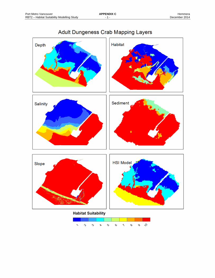
Port Metro Vancouver APPENDIX C Hemmera RBT2 – Habitat Suitability Modelling Study - 1 - December 2014

Port Metro Vancouver APPENDIX C Hemmera RBT2 – Habitat Suitability Modelling Study - 2 - December 2014
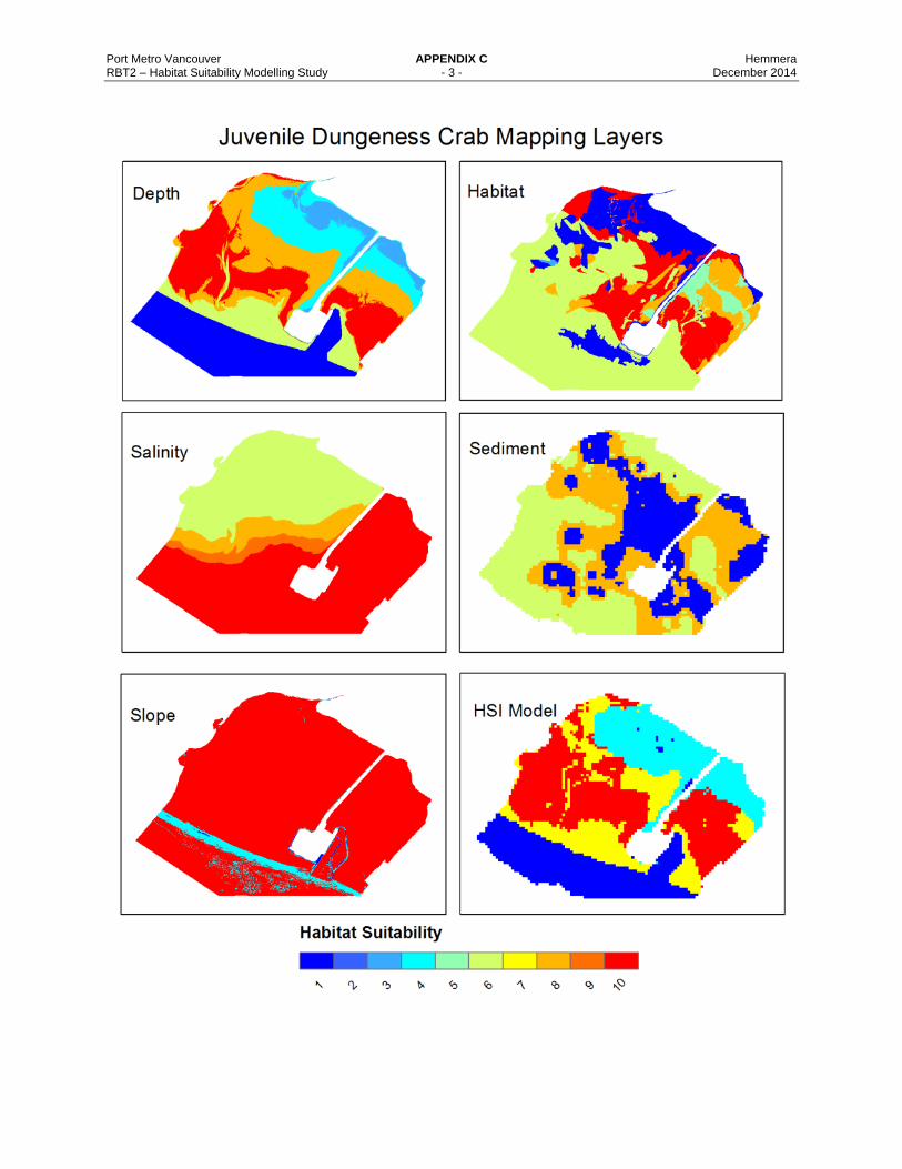
Port Metro Vancouver APPENDIX C Hemmera RBT2 – Habitat Suitability Modelling Study - 3 - December 2014

Port Metro Vancouver APPENDIX C Hemmera RBT2 – Habitat Suitability Modelling Study - 4 - December 2014
APPENDIX D
Table of SDM Parameter Outputs for the Sea Pen, Coefficient Estimate, Standard Error,
z-score, and p value

Port Metro Vancouver APPENDIX D Hemmera RBT2 – Habitat Suitability Modelling Study - 1 - December 2014
Coefficients Model Parameters
Estimate Std. Error z value Pr(>|z|)
(Intercept) -9.28401 0.39746 -23.36 <2e-16
Bottom Current Velocity -6.90673 0.23749 -29.08 <2e-16
Wave Height 17.79358 0.79796 22.3 <2e-16
Broad BPI 0.17827 0.00387 46.07 <2e-16
Fine BPI 0.64948 0.02643 24.57 <2e-16
APPENDIX 12-B
Rationale for Exclusion of Other Certain and
Reasonably Foreseeable Projects and
Activities in the Cumulative Effects
Assessment of Marine Invertebrates
PORT METRO VANCOUVER | Roberts Bank Terminal 2
This page is intentionally left blank
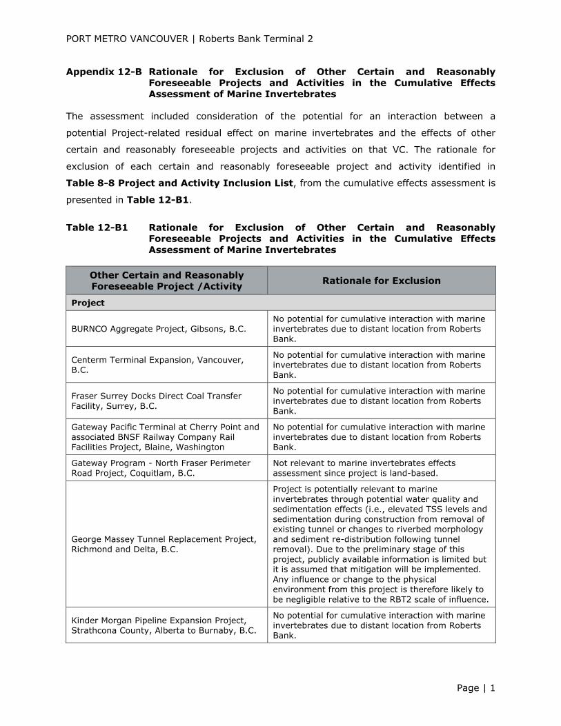
PORT METRO VANCOUVER | Roberts Bank Terminal 2
Page | 1
Appendix 12-B Rationale for Exclusion of Other Certain and Reasonably
Foreseeable Projects and Activities in the Cumulative Effects Assessment of Marine Invertebrates
The assessment included consideration of the potential for an interaction between a
potential Project-related residual effect on marine invertebrates and the effects of other
certain and reasonably foreseeable projects and activities on that VC. The rationale for
exclusion of each certain and reasonably foreseeable project and activity identified in
Table 8-8 Project and Activity Inclusion List, from the cumulative effects assessment is
presented in Table 12-B1.
Table 12-B1 Rationale for Exclusion of Other Certain and Reasonably Foreseeable Projects and Activities in the Cumulative Effects
Assessment of Marine Invertebrates
Other Certain and Reasonably Foreseeable Project /Activity
Rationale for Exclusion
Project
BURNCO Aggregate Project, Gibsons, B.C. No potential for cumulative interaction with marine invertebrates due to distant location from Roberts Bank.
Centerm Terminal Expansion, Vancouver, B.C.
No potential for cumulative interaction with marine invertebrates due to distant location from Roberts
Bank.
Fraser Surrey Docks Direct Coal Transfer
Facility, Surrey, B.C.
No potential for cumulative interaction with marine
invertebrates due to distant location from Roberts Bank.
Gateway Pacific Terminal at Cherry Point and
associated BNSF Railway Company Rail Facilities Project, Blaine, Washington
No potential for cumulative interaction with marine
invertebrates due to distant location from Roberts Bank.
Gateway Program - North Fraser Perimeter Road Project, Coquitlam, B.C.
Not relevant to marine invertebrates effects assessment since project is land-based.
George Massey Tunnel Replacement Project, Richmond and Delta, B.C.
Project is potentially relevant to marine invertebrates through potential water quality and sedimentation effects (i.e., elevated TSS levels and
sedimentation during construction from removal of existing tunnel or changes to riverbed morphology and sediment re-distribution following tunnel removal). Due to the preliminary stage of this
project, publicly available information is limited but it is assumed that mitigation will be implemented. Any influence or change to the physical
environment from this project is therefore likely to be negligible relative to the RBT2 scale of influence.
Kinder Morgan Pipeline Expansion Project, Strathcona County, Alberta to Burnaby, B.C.
No potential for cumulative interaction with marine invertebrates due to distant location from Roberts Bank.
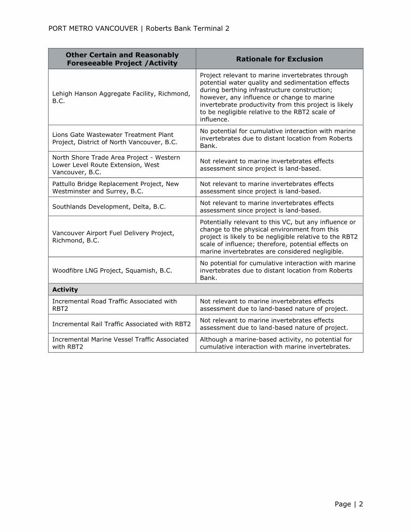
PORT METRO VANCOUVER | Roberts Bank Terminal 2
Page | 2
Other Certain and Reasonably
Foreseeable Project /Activity Rationale for Exclusion
Lehigh Hanson Aggregate Facility, Richmond, B.C.
Project relevant to marine invertebrates through potential water quality and sedimentation effects during berthing infrastructure construction;
however, any influence or change to marine invertebrate productivity from this project is likely to be negligible relative to the RBT2 scale of
influence.
Lions Gate Wastewater Treatment Plant
Project, District of North Vancouver, B.C.
No potential for cumulative interaction with marine
invertebrates due to distant location from Roberts Bank.
North Shore Trade Area Project - Western
Lower Level Route Extension, West Vancouver, B.C.
Not relevant to marine invertebrates effects assessment since project is land-based.
Pattullo Bridge Replacement Project, New Westminster and Surrey, B.C.
Not relevant to marine invertebrates effects assessment since project is land-based.
Southlands Development, Delta, B.C. Not relevant to marine invertebrates effects assessment since project is land-based.
Vancouver Airport Fuel Delivery Project, Richmond, B.C.
Potentially relevant to this VC, but any influence or change to the physical environment from this project is likely to be negligible relative to the RBT2 scale of influence; therefore, potential effects on
marine invertebrates are considered negligible.
Woodfibre LNG Project, Squamish, B.C.
No potential for cumulative interaction with marine
invertebrates due to distant location from Roberts Bank.
Activity
Incremental Road Traffic Associated with
RBT2
Not relevant to marine invertebrates effects
assessment due to land-based nature of project.
Incremental Rail Traffic Associated with RBT2 Not relevant to marine invertebrates effects assessment due to land-based nature of project.
Incremental Marine Vessel Traffic Associated with RBT2
Although a marine-based activity, no potential for cumulative interaction with marine invertebrates.


![[Appendix to Part ] Capital Adequacy Guidelines for Banks ...Appendix C, 12 CFR part 208, Appendix F, 12 CFR part 325, Appendix D, or 12 CFR part 567, Appendix C, to calculate its](https://img.dokumen.tips/doc/110x75/60009cd39f976b51951e917a/appendix-to-part-capital-adequacy-guidelines-for-banks-appendix-c-12-cfr.jpg)