Analytical Modelling of Microstructure Changes

ORIGINAL ARTICLE

Analytical modelling of microstructure changes

in the machining of 304 stainless steel

Lin Yan & Wenyu Yang & Hongping Jin & Zhiguang Wang

Received: 20 February 2011 /Accepted: 8 May 2011 /Published online: 24 May 2011# Springer-Verlag London Limited 2011

Abstract In the machining of hard machined materials,

microstructure changes in the machined surface must be

taken into account to improve product performance.

Therefore, a large number of experimental and finite

element method investigations have been carried out to

investigate these microstructure changes. However, until

now, only a few studies have reported the analytical

modelling of microstructure changes. This paper presents

a hardness-based analytical model that accounts for both

mechanical and thermal effects in predicting microstructure

changes during the machining of 304 stainless steel. The

model was also validated for a range of cutting speeds, feed

rates, and wear widths. The predicted results are in good

agreement with the experimentally measured results. Thus,

with the analytical model, an accurate prediction of

microstructure changes is achieved, which reduces experi-

mental expense and finite element method computational

time.

Keywords Tool flank wear width . Process parameters .

Dark layer .White layer

1 Introduction

In recent years, microstructure changes in the surface of a

machined workpiece, commonly referred to as white and

dark layers, have been studied under certain machining

conditions. Moreover, white and dark layers are generally

considered to be detrimental to fatigue life because they are

known to be hard and brittle.

Barbacki and Kawalec [1] studied dark and white layers

formed during the machining of steels and concluded that

the dark layer is not observed in high-speed machining due

to its high tempering temperature. Barry and Byrne [2] also

used transmission electron microscope (TEM) to analyse

white layers generated in hard turning of AISI 4340 steel

with worn and unworn tools. They found that under these

conditions, white layers can form if the temperature

exceeds the austenitic formation temperature of the steel.

Moreover, Ramesh et al. [3] carried out TEM, X-ray

diffraction (XRD), EDS, and nano-indentation hardness

tests of white layers formed from hard turning of AISI

52100 steel and found that cementite was absent in high-

speed machining in which thermal effects are expected to

be dominant. In contrast, cementite was observed in the

white layer formed at a low cutting speed, at which

mechanical effects tend to dominate and the temperatures

may not exceed the austenitisation temperature of the

steel.

In recent years, some attempts to numerically model the

microstructure changes have been reported. Ramesh et al.

[4] used a numerical model of orthogonal machining to

calculate the temperature, effective stress, and plastic strain

in a workpiece subsurface in ABAQUS, a finite element

software. In his work, the white layer was formed at a depth

L. Yan :W. Yang (*) :H. Jin : Z. Wang

Department of Mechanical Science and Engineering,

Huazhong University of Science and Technology,

1037 Luoyu Road,

Wuhan, China

e-mail: [email protected]

L. Yan

e-mail: [email protected]

L. Yan :W. Yang

State Key Laboratory of Digital

Manufacturing Equipment and Technology,

Wuhan, China

Int J Adv Manuf Technol (2012) 58:45–55

DOI 10.1007/s00170-011-3384-5

where the estimated temperature exceeds the austenitisation

temperature in the machining of 52100 steel. Hence, their

study was conducted under thermally dominant cutting

conditions that promote phase transformation. A finite

element model was also proposed by Umbrello and Jawahir

[5] to study the orthogonal cutting process on hardened

AISI 52100. The proposed model was properly calibrated

by means of an iterative procedure based on experimental

data, which included chip geometry, cutting forces, temper-

atures, and white layer. As an improvement, Umbrello and

Jawahir [6] presented a new finite element model for

microstructure changes, referred to as white and dark

layers. In their work, both a hardness-based flow stress

and empirical models for describing the white and dark

layer formation were developed by using the finite element

method.

For the analytical modelling of the microstructure

changes, Chou and Song [7] developed an analytical model

to predict the cutting temperature distribution, particularly

at the machined surfaces. They proposed that the white

layer forms when the workpiece temperature exceeds the

austenitisation temperature. Song [8] also used the austeni-

tisation temperature to predict the depth of the white layer

in the machining of 52100 hardened steel. However, Han

[9] classified the major mechanisms that cause microstruc-

ture changes in various processes into two categories:

thermal and mechanical. From this, it follows that the

previous modelling efforts are based on the hypothesis that

the thermal effect is predominantly responsible for the

formation of the white layer, which ignores the mechanical

effects.

The main goal of this paper is to develop a hardness-

based analytical model that accounts for both mechanical

and thermal influences. First, a new analytical model for

predicting the machining temperature is developed in dry

cutting. Second, the measured results of temperature,

hardness, and microstructure changes are used to determine

the temperature of the microstructure changes. Third, the

analytical model of white and dark layer formation is

provided and validated. Finally, the effects of the machin-

ing conditions are analysed for a range of cutting speeds,

feed rates, and tool flank wear widths.

2 Experimental and analytical study

Machining experiments were performed on a lathe in the

orthogonal machining of a 304 stainless steel tube. Kistler

9257 cutting force dynamometer and an infrared thermal

measurement camera VarioCAM were used to measure the

forces and cutting temperature distribution, respectively.

The experimental results of temperature distribution along

the tool-workpiece interface were used to determine the

heat partition coefficient along the tool flank wear width,

and a new analytical model was developed to determine the

machining temperature distribution.

2.1 Experimental setup

For studying the effect of tool flank wear widths on the

machining temperature and forces, three cutting tools with

prefabricated wear widths of 0.3, 0.5, and 1 mm, respec-

tively were used. The experimental setup is shown in

Fig. 1.

In these experiments, the Kistler 9257 has a minimum

resolution of 2 N, which is a three-component tool holder

dynamometer. David et al. [10] noted that the actual forces

are the summation of the forces due to the wear and the

fresh-tool cutting forces when tool flank wear is absent. To

determine the aforementioned forces, fresh and prefabri-

cated wear width tools with the same parameters but

different wear widths were used in these experiments.

Saoubi and Chandrasekaran [11] used an infrared

thermal imaging camera to measure the cutting temperature

distribution on the cutting tool, and the results were further

used to validate a proposed model in the analytical

modelling of the temperature. Hence, an infrared thermal

imaging camera (VarioCAM) was also used to measure the

temperature distributions in the present work. The camera

used in this paper is a modern thermographic system for

precise, quick, and non-contact measurement of the surface

temperatures of objects. Moreover, its compact, robust

Fig. 1 The experimental setup for measuring the machining temper-

ature and forces

46 Int J Adv Manuf Technol (2012) 58:45–55

design and high degree of protection make it especially

suitable for industrial applications, even under unfavourable

external conditions. The infrared thermal measuring camera

has 640×480 or 384×228 pixels of array size, a target

image temperature range between −40°C and 1,200°C, and

a minimum resolvable temperature difference of approxi-

mately 0.2°C.To study the machining area temperature

distribution along the tool flank wear width, the infrared

camera was placed sufficiently close to the cutting zone at a

distance of 40 mm [12–14]. Two chips of silicon with a

thickness of 0.5 mm each were placed in front of the

camera to protect the camera lens, while the other areas

were protected using Plexiglas, which is IR-proof. The

camera was placed on a small pallet of the lathe, which

moved with the cutting tool at all times. The cutting

experiments were performed at three different cutting

speeds (100, 150, and 175 m/min) and three different feed

rates (0.1, 0.15, and 0.2 mm/rev). The length of feed in

every experiment was limited to 5 mm to minimise the

variability of a new cutting tool and to avoid introduction of

new tool wear. A new cutting tool was used for each

experimental parameter.

2.2 Measurements

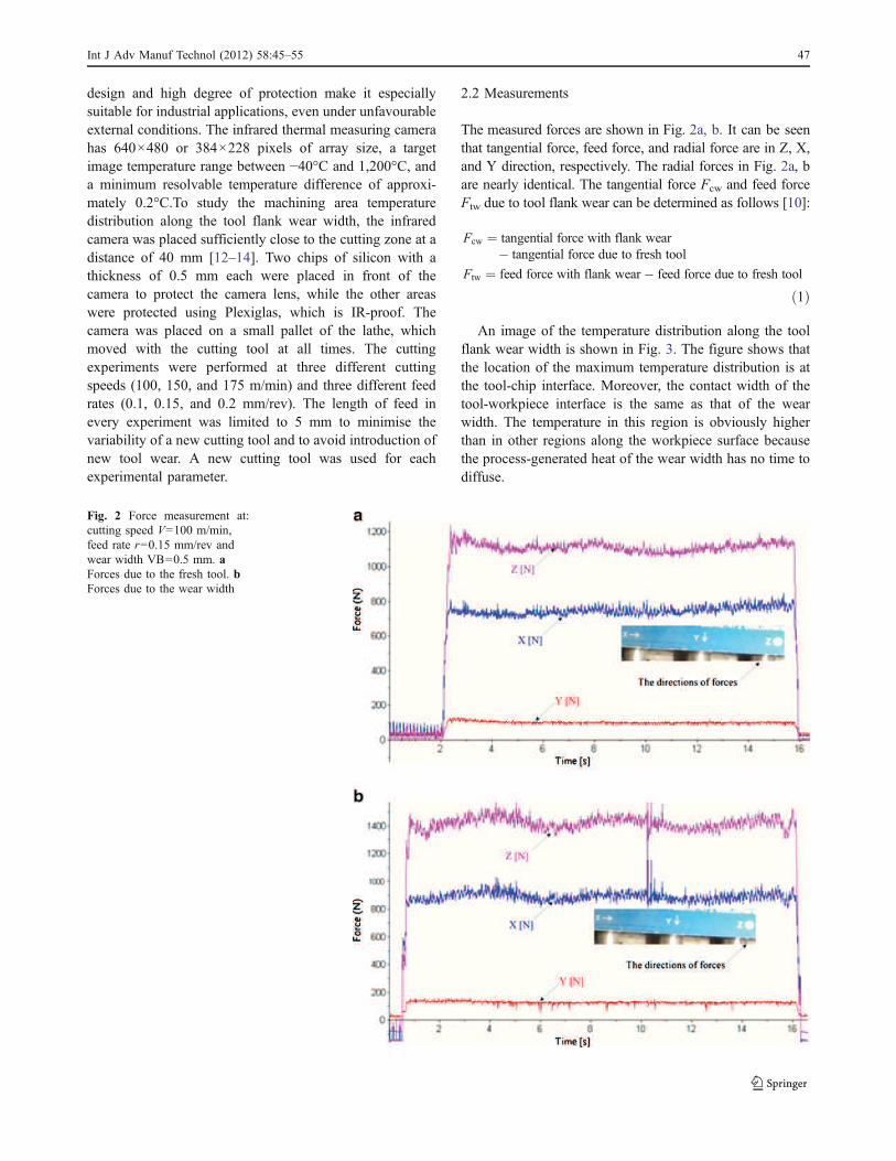
The measured forces are shown in Fig. 2a, b. It can be seen

that tangential force, feed force, and radial force are in Z, X,

and Y direction, respectively. The radial forces in Fig. 2a, b

are nearly identical. The tangential force Fcw and feed force

Ftw due to tool flank wear can be determined as follows [10]:

Fcw ¼ tangential force with flank wear

" tangential force due to fresh tool

Ftw ¼ feed force with flank wear " feed force due to fresh tool

ð1Þ

An image of the temperature distribution along the tool

flank wear width is shown in Fig. 3. The figure shows that

the location of the maximum temperature distribution is at

the tool-chip interface. Moreover, the contact width of the

tool-workpiece interface is the same as that of the wear

width. The temperature in this region is obviously higher

than in other regions along the workpiece surface because

the process-generated heat of the wear width has no time to

diffuse.

Fig. 2 Force measurement at:

cutting speed V=100 m/min,

feed rate r=0.15 mm/rev and

wear width VB=0.5 mm. a

Forces due to the fresh tool. b

Forces due to the wear width

Int J Adv Manuf Technol (2012) 58:45–55 47

2.3 Modelling the cutting temperature rise on the workpiece

machining surface

In modelling, the temperature rise of the machining surface,

two heat sources are assumed to exist, as shown in Fig. 4

[15]. The first is the primary heat source of the shear plane,

and the second is the rubbing heat source at the tool-

workpiece interface. The temperature rise of the workpiece

surface and subsurface is obtained by superposition of the

two heat sources.

In this model, the shear heat source is an oblique band

heat source that moves beneath the workpiece surface with

a velocity V. Just opposite the shear zone is an imaginary

and extended heat source for continuity in modelling.

Compared to stainless steel, the atmosphere is considered to

be insulating. Therefore, the external surfaces of the

workpiece and chip are considered to be insulated in this

study. The imaginary heat source with the same heat

intensity as the shear heat source is applied in this model.

The temperature rise at any point M(x,z) due to the oblique

heat source and imaginary heat source [16] under the

thermal diffusivity a of 304 stainless steel are determined

by the work of Graves et al. [17]. A compilation and

rigorous analysis of the thermal conductivity of 304

stainless steel between 300 and 1,000 K and the thermal

diffusivity from 297 to 432 K is given in their work. After

careful evaluation, the models of thermal conductivity and

thermal diffusivity are given as follows:

kw ¼ 7:9318þ 0:023051 & K " 6:4166& 10"6 & K2

a ¼ 3:0246& 10"2 þ 1:9016& 10"5 & K þ 1:7244& 10"8 & K2

ð3Þ

The modified Bessel function k0(u) is determined by:

k0ðuÞ ¼1

2

Z 1

0

dw

wexp "w"

u2

4w

" #

ð4Þ

A similar application of a moving heat source is used to

determine the temperature rise due to the rubbing heat

source. The rubbing heat source between the tool flank

wear width and workpiece surface is treated as a band heat

source, which moves along the workpiece surface on a

semi-infinite body surface with velocity V. The boundary

condition of the workpiece surface is considered insulated

in this study. An imaginary heat source of the rubbing heat

source is used to calculate the temperature rise at the

workpiece surface, overlapping with the initial heat source.

The temperature rise of the workpiece surface and

subsurface due to the rubbing heat source is given by

TrubbingðX ;ZÞ ¼1

2pkw

Z

VB

0

BðxÞqrubbing expðX " xÞV

2a

$ %

& K0

V

2a

ffiffiffiffiffiffiffiffiffiffiffiffiffiffiffiffiffiffiffiffiffiffiffiffiffiffiffiffi

ðX " xÞ2 þ Z2

q

$ %

dx ð5Þ

Fig. 3 Temperature measurement at: cutting speed V=100 m/min,

feed rate r=0.15 mm/rev and wear width VB=0.5 mm

Fig. 4 Heat transfer model and heat partition along the tool-workpiece

interface


appropriate co-ordinate system can be expressed as follows:

Tshear x; zð Þ ¼qshear

2pkw

Z

L

0

expX " x sinϕð ÞV

2a

$ %

K0

V

2a

ffiffiffiffiffiffiffiffiffiffiffiffiffiffiffiffiffiffiffiffiffiffiffiffiffiffiffiffiffiffiffiffiffiffiffiffiffiffiffiffiffiffiffiffiffiffiffiffiffiffiffiffiffiffiffiffiffiffiffiffiffi

X " x sinϕð Þ2 þ Z " x cosϕð Þ2q

$ %(

þK0

V

2a


X " x sinϕð Þ2 þ Z þ x cosϕð Þ2q

$ %)

dx

ð2Þ

where ϕ ¼ f" p2; L ¼

tcsin f

, f is the shear angle, tc is the

uncut chip thickness, and the thermal conductivity kw and

The heat intensity of the shear heat source qshear and the

heat intensity of the rubbing heat source qrubbing are given

by [18]

qshear ¼Fc cos f" Ft sin fð Þ V cos a= cos f" að Þð Þ

tcw csc fð6Þ

qrubbing ¼FcwV

wVBð7Þ

where VB is the tool flank wear width, w is the width of cut,

and Fc and Ft are the tangential and feed forces of a fresh

tool, respectively. Here, the model uses the measured

tangential and feed forces with and without tool wear as

inputs. The forces are used to estimate the heat intensities

generated on the shear plane and the flank wear width. The

temperature rise on the workpiece surface and subsurface

during machining is given by

TMðX ;ZÞ ¼ TrubbingðX ;ZÞ þ Tshear ð8Þ

Previous works have demonstrated that the machining

temperature distribution along the tool flank wear width can

be measured by an infrared thermal camera, shown in

Fig. 3. The temperatures at different points along the width

were observed by using the software of this camera

measuring system. Equation 8 can be further expressed as

follows:

TrubbingðX ;ZÞ ¼ TMðX ;ZÞ " Tshear ð9Þ

Let

Trubbingðx;zÞ ¼1

2pkw

Z

VB

0

BðxÞqrubbing expðX " xÞV

2a

$ %

& K0

V

2a


ðX " xÞ2 þ Z2

q

$ %

dx

¼X

n

i¼0

B xið Þ1

2pkwqrubbing exp

ðX " xiÞV

2a

$ %

& K0

V

2a

ffiffiffiffiffiffiffiffiffiffiffiffiffiffiffiffiffiffiffiffiffiffiffiffiffiffiffiffiffi

ðX " xiÞ2 þ Z2

q

$ %

¼ B x0ð Þf x0ð Þ þ B x2ð Þf x2ð Þ þ . . .þ B xnð Þf xnð Þ

ð10Þ

Thus,

B x0ð Þf x0ð Þ þ B x2ð Þf x2ð Þ þ . . .þ B xnð Þf xnð Þ ¼ TMðx;zÞ " Tshearðx;zÞ

ð11Þ

where xi ¼ ihði ¼ 0; 1; 2 . . . nÞ h ¼ VBn, and the tool-workpiece

interface heat partition coefficient at different points along

tool flank wear width B x0ð Þ;B x2ð Þ . . .B xnð Þ½ ) can be

obtained under different cutting conditions. From the

calculated results, the heat partition coefficient has an

approximate relationship of the following form:

BðxÞ ¼ "0:7341xþ 0:8825 x 2 0;VB½ ) ð12Þ

where x is the distance from the cutting edge.

Thus

Using the above equation, the temperature rise at any

point in the workpiece can be determined, thereby

simplifying the calculation processing compared to the

work of Han [9] without a matching computation of the

heat partition coefficient along the tool-workpiece interface.

The calculated results of the temperature distribution in the

workpiece are shown in Fig. 5a–c. The wear widths have a

noticeable influence on the temperature distribution. For

different wear widths, the location of the largest tempera-

ture difference is at the cutting edge under these machining

conditions. The reason why such a large difference is

generated is because of the effect of the second heat source

between the tool and chip interface, which is ignored in

determining the temperature distribution.

2.4 Determination of microstructure changes temperature

Optical microscopy was used to analyse the white and dark

layers generated under different machining conditions, and

the micrographs of these layers are shown in Fig. 6. The


TMðx;zÞ ¼ Trubbing þ Tshear ¼1

2pkw

Z

VB

0

"0:7341xþ 0:8825ð Þqrubbing expX " xð ÞV

2a

$ %

& K0

V

2a


X " xð Þ2 þ Z2

q

$ %

dx

þqshear

2pkw

Z

L

0

expðX " x sinϕÞV

2a

$ %

K0

V

2a


X " x sinϕð Þ2 þ Z " x cosϕð Þ2q

$ %

þ K0

V

2a


X " x sinϕð Þ2 þ Z þ x cosϕð Þ2q

$ %( )

dx

ð13Þ

white and dark layers are all present at the following cutting

condition. The depth of the white layer also increased with

an increase in the wear width.

The hardness of the surface and subsurface layers was

measured, and the results are shown in Fig. 7a, b. From the

figures, we find that the hardness of the bulk material is

240 HV, and for different widths of 0.1, 0.3, and 0.5 mm,

the total depths of the white and dark layers are 0.515,

0.572, and 0.643 mm, respectively. Comparing Fig. 6 with

Fig. 7, the range of the white layer hardness is 360 HV<

WL<400 HV, and the depth of the white layer is about 0.1

and 0.158 mm at wear widths of 0.3 and 0.5 mm,

respectively. Comparing Fig. 5 with Fig. 7, the temperature

at which the microstructure change occurs is approximately

230°C. It is worth pointing out that the temperature of

Fig. 5 Temperature rise in the workpiece during machining at different

wear widths VB (cutting speedV=100 m/min and Feed rate r=0.15 mm/

rev). a VB=0.1 mm, b VB=0.3 mm, c VB=0.5 mm

Fig. 6 Microstructure changes generated at cutting speed V=100 m/min

and feed rate r=0.15mm/rev: a VB=0.3 mm tool flank wear width, ×400;

b VB=0.5 mm tool flank wear width, ×800


transformation in predicting white and dark layer formation

proposed in this research was based on both mechanical

and thermal effects.

3 Calculation of white and dark layers formation

and model validation

3.1 Calculation of white and dark layer formation

To develop an analytical model for white and dark layer

formation, a flow chart of the calculation is shown in Fig. 8,

which was conducted over a wide range of cutting

parameters and wear widths. This model is based on a

hardness modification [6], which represents mechanical and

thermal effects. In this flow chart, three steps are involved:

1. The temperatures in different layers are checked for

each step.

2. The hardness of the different layers is updated and

stored.

3. The final step is to model the white layer and dark layer

based on the determined hardness.

HVinitial is the initial Vickers Hardness of the 304 stainless

steel, and the increment in hardness ΔHV is given by:

ΔHV¼ J & HVp"HV+ ,

= Tp"Tmicro"changes

+ ,

& T"Tmicro"changes

+ ,+ ,

ð14Þ

Fig. 7 Experimental hardness on

machined surfaces at different

wear width (cutting speed

V=100 m/min and feed rate

r=0.15 mm/rev), a wear width

VB=0.3 mm; b wear width

VB=0.5 mm


where Tmicro-changes is the temperature of microstructure

changes occur, and T is the current temperature in the layer.

The parameters J, HVp, Tp are found by experiments in

different cutting conditions, and the final equation of

hardness increment is shown as:

ΔHV ¼ 13:82& ð 400" HVð Þ= 905" Tmicro"changes

+ ,

& T " Tmicro"changes

+ ,,

ð15Þ

During the procedure, the highest hardness of the different

layers is stored until the effect of the tool wear width is gone. It

should be pointed out that the model is only suitable for the

workpiece material in which the machined hardness decreases

from the surface to the bulk, i.e., the dark layer is harder than

the bulk. Therefore, when the subsurface hardness of the

material is less than the bulk [19], the model is invalid.

3.2 Model validation

The presence of martensite on the machined surface has

been confirmed by XRD, and the spectra are shown in

Fig. 9. The transformations of the machined surfaces are

depicted; γ and α represent the austenite and martensite

phases, respectively. The figure shows that the austenite

Fig. 9 XRD spectra of a the

un-machined surface;

b machined surfaces at cutting

speed V=100 m/min, wear

width VB=0.3 mm and feed

rate r=0.15 mm/rev

Fig. 8 Flow chart of the white and dark layer calculation


near the machined surface transformed to martensite. This

result was also found by Ghosh [20].

The measured and predicted micro-hardness values are

shown in Fig. 10 under the same machining conditions. The

largest errors absolute are acceptable at 9%. The variation

in hardness shows that the white layer is much harder than

both the dark layer and bulk material. Moreover, the dark

layer is also harder than the bulk material. These variations

in hardness are related to the microstructure phase

transformation from austenite to martensite; the latter is

harder. However, the predicted hardness is less than the

measured hardness. This discrepancy results from neglecting

the tool-chip heat source in determining the machining

temperature distribution, which makes the predicted tempera-

ture less than the experimental value.

4 Analysis of the white and dark layer formation

In this section, the influence of the cutting parameters and

wear widths on the white and dark layer formation will be

discussed. In particular, three levels were considered for

each parameter: 100, 150, and 175 m/min for the cutting

speed; 0.1, 0.15, and 0.2 mm/rev for the feed rates; and 0.1,

0.3, and 0.5 mm for the wear widths.

4.1 Influence of the cutting speeds

As seen in Fig. 11, the influence of cutting speed on the

microstructure modifications is evident. In general, higher

cutting speeds cause deeper white layer formation, at least

in a range from 100 to 175 m/min. Therefore, when large

Fig. 11 White and dark layer formation for different cutting speeds at

wear width VB=0.3 mm and feed rate r=0.15 mm/rev

Fig. 10 Predicted andmeasuredmicrostructure hardness at cutting speed

V=100 m/min, wear width VB=0.3 mm and feed rate r=0.15 mm/rev

Fig. 12 White and dark layer formation for different feed rates at

cutting speed V=100 m/min and wear width VB=0.3 mm

Fig. 13 White and dark layer formation for different wear widths at

cutting speed V=100 m/min and feed rate r=0.15 mm/rev


cutting speeds are utilised, zones deeper in the material

reach a temperature that is high enough to cause the phase

transformation of the white layer, resulting in a greater

white layer thickness [5]. In contrast, by increasing the

cutting speed, the dark layer depth decreases. This is due to

the heat-affected zone, i.e., the temperature rises with the

cutting speed, while the zone decreases. Due to the decrease

in area of the zone, the region over which the temperature

ranges with the white layer and dark layer decreases;

consequently, a reduced dark layer is observed.

4.2 Influence of feed rate

The influence of feed rate on the microstructure changes

was studied at a constant cutting speed and wear width. As

seen in Fig. 12, the thickness of the white layer increases

with increasing feed rate, and this variation is more evident

when a higher feed rate is utilised; in contrast, the dark

layer decreases slightly. In fact, it is well known that the

temperature rises with the feed rate, and the heat-affected

zone also increases. However, when higher feed rates are

utilised, deeper zones with a white layer can be observed.

In contrast, because the heat- affected zone thickness

increases slightly, the size of the dark layer tends either to

remain unchanged or decrease slightly.

4.3 Influence of the wear width

The influence of the wear width on the microstructure

changes was investigated, keeping both the cutting speed

and feed rate constant. As shown in Fig. 13, the depth of

the white layer increases with increasing wear width.

Moreover, the depth of the dark layer decreases, and this

variation is more evident when a severe wear width is used.

This variation is due to the heat-affected zone and the

maximum temperature reached during machining. A larger

width produces higher temperature, a deeper heat-affected

zone, and a longer friction distance. Therefore, when a

larger width is used, deeper microstructure changes can be

observed.

5 Conclusions

In this paper, a micro-hardness-based model was developed to

analytically study the turning process in terms of white and

dark layer formation. The following conclusions can be drawn:

1. The good agreement obtained between the experimental

and analytical results indicate that the proposed micro-

hardness-based model was suitable in identifying the

microstructure changes at various depths below the

machined surface.

2. Based on the experimental observations of the infrared

thermal images and forces, we can conclude that the

machining experiment designed is suitable in studying the

effect of tool flank wear width on the workpiece surface.

3. As a contribution, the new model of machining

temperature distribution proposed here simplified the

computational effort with good accuracy by avoiding

the corresponding computation of a heat partition

coefficient at the tool-workpiece interface.

4. Thewhite layer is much harder than the both the dark layer

and the bulk material, and the dark layer is harder than the

bulk material, which is a key observation of this study.

5. The white layer increases with increasing cutting speed,

feed rate, and wear width. In contrast, the depth of the

dark layer decreases with increasing cutting speed, feed

rate, and wear width.

6. In addition, the proposed micro-hardness-based model

could be used to research the residual stress distribution

and to select the process parameters rapidly in order to

achieve a more desirable final surface integrity with

acceptable accuracy.

Acknowledgement This work has been funded by a grant from the

Major State Basic Research Development Program of China (973

Program, NO.2009CB724306).

References

1. Barbacki A, Kawalec M (1997) Structural alterations in the

surface layer during hard machining. J Mater Process Technol

64:33–39

2. Barry J, Byrne G (2002) TEM study on the surface white layer in

two turned hardened steels. Mater Sci Eng A 325:356–364

3. Ramesh A, Melkote SN, Allard LF, Riester L, Watkins TR (2005)

Analysis of white layers formed in hard turning of AISI 52100

steel. Mater Sci Eng A 390:88–97

4. Ramesh A (2002) Prediction of process-induces microstructure

changes and residual stresses in orthogonal hard machining. PhD

thesis, Mechanical Engineering, Georgia Institute of Technology.

5. Umbrello D, Jawahir IS (2009) Numerical modeling of the

influence of process parameters and workpiece hardness on the

white layer formation in AISI 52100 steel. Int J Adv Manuf

Technol 44:955–968

6. Domenico U (2010) Influence of material microstructure changes

on surface integrity in hard machining of AISI 52100 steel. Int J

Adv Manuf Technol. doi:10.1007/s00170-010-3003-x

7. Chou YK, Song H (2005) Thermal modeling for white layer

predictions in finish hard turning. Int J Mach Tools Manuf

45:481–495

8. Song H (2003) Thermal modeling for finish hard turning. PhD

thesis, Mechanical Engineering, University of Alabama.

9. Han S (2006) Mechanisms and modeling of white layer formation

in orthogonal machining of steels. PhD thesis, Mechanical

Engineering, Georgia Institute of Technology.

10. David WS, Shiv KG, Richard ED (2001) A new mechanistic

model for predicting worn tool cutting forces. Mach Sci Technol

5:23–42


11. M’Saoubi R, Chandrasekaran H (2011) Experimental study and

modeling of tool temperature distribution in orthogonal cutting of

AISI 316 L and AISI 3115 steels. Int J Adv Manuf Technol.

doi:10.1007/s00170-011-3257-y

12. Kazban RV, Vernaza KM, Mason JJ (2008) Measurements of

forces and temperature fields in high-speed machining of 6061-T6

aluminum alloy. Exp Mech 48:307–317

13. Sullivan DO, Cotterell M (2002)Workpiece temperature measurement

in machining. Proc IME B J Eng Manufact 216:135–139

14. Dinca C, Lazoglu I, Serpenguzel A (2008) Analysis of thermal

fields in orthogonal machining with infrared imaging. J Mater

Process Tech 198:147–154

15. Huang Y (2002) Predictive modeling of tool wear rate with

application to CBN hard turning. PhD thesis, Mechanical

Engineering, Georgia Institute of Technology.

16. Komanduri R, Hou ZB (2000) Thermal modeling of the metal

cutting process Part I—temperature rise distribution due to shear

plane heat source. Int J Mach Tools Manuf 42:1715–1752

17. Graves RS, Kollie TG, McElroy DL, Gilchrist KE (1991) The

thermal conductivity of AISI 304 L stainless steel. Int J

Thermophys 12:409–415

18. Hanna CR (2007) Engineering residual stress into the workpiece

through the design of machining process parameters. PhD thesis,

Mechanical Engineering, Georgia Institute of Technology.

19. Umbrello D, Filice L (2009) Improving surface integrity in

orthogonal machining of hardened AISI 52100 steel by modeling

white and dark layers formation. Ann CIRP 58:73–76

20. Ghosh S, Kain V (2010) Microstructure changes in AISI 304 L

stainless steel due to surface machining: effect on its susceptibility

to chloride corrosion cracking. J Nucl Mater 403:62–67


Copyright of International Journal of Advanced Manufacturing Technology is the property of Springer Science

& Business Media B.V. and its content may not be copied or emailed to multiple sites or posted to a listserv

without the copyright holder's express written permission. However, users may print, download, or email

articles for individual use.

Documents

Analytical Modelling of Microstructure Changes