ANALYTICAL AND COMPUTATIONAL MODELLING OF GO-KART …

www.tjprc.org SCOPUS Indexed Journal [email protected]

ANALYTICAL AND COMPUTATIONAL MODELLING OF GO-KART

POWERTRAINS

HITESH KUMAR*, KUNAL MATHUR & ADITYA NATU

Department of Mechanical Engineering, Delhi Technological University, Delhi, India

ABSTRACT

In this study, we have a unique methodology of developing two types of transmission systems for a go-kart with known

specifications depicted and compared later on. The two different forms of transmission systems are viz. manual

transmission (with a fixed gearbox) and semi-automatic transmission (with a belt and pulley based CVT or Continuous

Variable Transmission). These designs were later validated by fatigue analysis using CAE (Computer Aided Engineering).

The detailed methodology also describes how the two systems have been compared on the basis of their performance on

the Go-kart in terms of acceleration (using analytical and computational approaches), intensity of the design-calculation

process and several other theoretical factors. The analytical approach computes the time taken by the go-kart (with both

the transmissions individually) to accelerate to its top speed using simultaneous differential equations that incorporate

rolling resistance. Computational approach achieves the same purpose by physical modelling of the entire go-kart

powertrain using MATLAB Simscape that solves complex dynamic equations while considering multiple derating factors.

The correlation between the analytical and computational results of a particular driveline is used to validate the

simulations performed and the assumptions made.

KEYWORDS: Powertrain, Go-kart; CVT, Simulink; Ansys & MATLAB

Received: Jun 08, 2020; Accepted: Jun 29, 2020; Published: Sep 30, 2020; Paper Id.: IJMPERDJUN20201463

1. INTRODUCTION

Go-karts are self-propelled, low ground clearance vehicles without a differential and suspension system. Go-karts

are widely used these days for recreational or racing purposes. Nowadays there are a lot of student teams in India as

well as abroad that design and fabricate racing Go-karts to compete in national/international level competitions. As

far as the transmission system is concerned, the students are given a choice of either proceeding with a completely

manual transmission or a CVT based transmission system. This study hence lays out a methodology of developing

and comparison of the two most popular transmission systems and compares them on a wide range of parameters

for a given Go-kart. With this design and comparison methodology, student teams can easily see which type of

transmission system will benefit their Go-kart designs, hence enabling them to take such major decisions in a proper

and a justifiable way.

A racing Go-kart was designed and manufactured in [1] by us and this study uses a lot of our experience

gained during the same. The methodology of development and comparison of both the drivelines (manual and semi-

automatic) on a particular Go-kart has been demonstrated by using the Go-kart in [1] as an example. Using the

vehicle parameters as given values, the designs of most of the powertrain components were made using machine

design equations, CAD modelling in SolidWorks, Siemens UGNX-11.0 and improving the designs by pushing them

through fatigue analysis performed using modern CAE tools like Ansys Workbench. Other powertrain components

Orig

ina

l Article

International Journal of Mechanical and Production

Engineering Research and Development (IJMPERD)

ISSN(P): 2249-6890; ISSN(E): 2249-8001

Vol. 10, Issue 3, Jun 2020, 15343-15370

© TJPRC Pvt. Ltd.

15344 Hitesh Kumar, Kunal Mathur & Aditya Natu

Impact Factor (JCC): 8.8746 SCOPUS Indexed Journal NAAS Rating: 3.11

were selected according to the vehicle requirements and available market standards. The design objectives of the

powertrain components of both the systems were kept the same for the sake of comparison. While comparing the

performance of the two systems on the basis of vehicle performance i.e. acceleration, two techniques for achieving the

same were devised. The first method was the analytical method that involved the solving of simultaneous differential

equations for calculating the time required for the vehicle to reach its top speed from rest using both the powertrain

systems individually in MATLAB Simulink 2018. The second method was the computational method in which the entire

physical models of both the transmission systems were developed in MATLAB Simscape. The models tend to simulate the

actual powertrain systems with a sufficient degree of accuracy and involve much more parameters than in the analytical

methods. The correlation between the results of both the methods suggested the validity of the simulation approach and

assumptions throughout the study. Finally the difference between the two transmission systems were summarized including

a bunch of theoretical parameters as well.

In [1], a racing Go-kart using a chain sprocket in the fixed gearbox (manual) transmission was designed, analyzed

and manufactured. In [2], another racing Go-kart has been manufactured using a CVT instead of a manual transmission. As

per [2], with the help of a CVT, constant step-less acceleration from start to high speed eliminates shift shock, gives better

fuel economy and less emissions. The authors of [3] have used a CVT as well as a chain drive, deploying the advantages of

the semi-automatic transmission system as in [2]. Chain drive is used because it is capable of taking shock loads and CVT

would provide automatic speed ratio change. The authors of [4] have implemented a chain drive instead of a CVT. For this

system, chain drive type transmission is most preferable as it is easy to install, simple in design and cost effective [4]. The

authors of [6] have discussed the differences between the performance of a manual transmission versus that of an

automatic transmission using a CVT in terms of vehicle velocity and gear shift shocks. Hence a comparison study of both

the transmission systems is shown by them.

[1], [2], [3] and [4] have not analysed the effect of the different transmission systems on their vehicle performance

before proceeding with their actual drivelines. Thereby alternate methods of transmission were not discussed and tested in

detail, whereas in this paper we are comparing whether the go-kart performance will be better in case of a CVT or manual

driveline. Authors of [8] have not compared the two transmission systems in terms of actual numerical vehicle parameters

such as acceleration, power delivered and respective weights, which we have managed to incorporate in our study. We

have also modelled the rolling resistance as a function of tire pressure and as a parabolic function of the Go-kart speed

while computing the acceleration in both the cases. This enabled us to perform continuous solving of the acceleration

functions using MATLAB Simulink to obtain accurate results. The authors of [7] have done a comparison study between a

manual transmission and a CVT based transmission in terms of acceleration; however they have not included the time

taken for gear shifting in case of manual transmission and have neglected rolling resistance as well, which we have

successfully worked upon. Moreover we have modelled the slip between the tire and the ground using standard referenced

values, which has not been pressed upon by the above papers that were studied for literature review. [6] and [7] did not

support their comparison study with precise physical modelling that we have done using MATLAB Simscape, which

includes various dynamic parameters that help simulate the entire powertrain systems. These papers also did not focus on

the different design challenges involved while incorporating either one of the powertrain systems, which we have managed

to complete using market selection, CAD modelling and fatigue analysis for both the systems respectively.

2. METHODOLOGY DEPICTION

Analytical and Computational Modelling of Go-Kart Powertrains 15345


This section depicts the entire methodology for designing, simulating and comparing the two transmission cases.

2.1. Selection Of Common Parameters for both the Powertrain Systems

The manual transmission with the fixed gearbox case was designed, manufactured and physically implemented by us in

[1], but slight changes would be made in the designs for the sake of using the same mathematical design equations. For the

second case, a CVT compatible engine is selected from the market on the basis of availability, cost and similarity of

technical specifications with the Honda Stunner engine used in [1]. The following are the general parameters that will stay

common for both the drivelines.

Table 1: List of Parameters that are Common for both the Drivelines

S. No. Symbol Description Values

1 m Mass of the go-kart 160kg

2 v Maximum go-kart speed (design target) 90kmph

3 wf Fraction of static weight towards the front of the vehicle 0.37

4 wr Fraction of static weight towards the rear of the vehicle 0.63

5 rg Radius of the go-kart wheel 0.1397m

6 g Acceleration due to gravity 9.8m/s2

7 S Slip ratio 1.25

8 d Deceleration of the vehicle 0.7g

9 Lwb Wheelbase of the go-kart 1.1m

10 hcg Height of the centre of gravity of the vehicle 0.1504m

11 Tb Braking torque by the braking system 153.58Nm

12 td Stopping time of the vehicle from 70kmph 3 seconds

13 μ Coefficient of friction between road and tyres 0.85 (asphalt)

14 ωemax1 Maximum engine speed 10000rpm

15 ωp1 Engine speed at maximum power 8000rpm

16 Te1 Maximum engine torque 11Nm

17 ωt1 Engine speed at maximum torque 6250rpm

18 Pr1 Primary reduction ratio 3.35

19 Gi ith gear ratio(i=1,2,3,4 or 5) Variable

Instead of aiming to design the vehicle for 70kmph as in [1], our aim would be as high as 90kmph because of

unpredictable friction losses in the engine as well as in the driveline components. This intuition is based on our experience

of manufacturing and designing go-karts. There should be a sufficient slip between the rear wheels and the ground to

provide better drive control as stated in [15]. Hence the slip percentage was chosen to be 20% (0.2) for dry asphalt at

μ=0.85 (shown in figure 3 of [15]). This implies that the ratio of the translation velocity of the rear wheels to that of the

vehicle would be equal to 1.25.

Hence S = 1.25. This value would be used throughout the study for both the transmission cases. Figure 3 of [15]

shows the sweet spot range within which the slip percentage must be kept as the slip dynamics is swift and at any value

after the peak of the friction curve is an open loop unstable [15].

2.2. Manual Transmission Case

This section would discuss the entire development and modelling using analytical and computational techniques of the

powertrain system of the manual transmission go-kart so that it can be compared with its semi-automatic counterpart in the

later sections.



2.2.1. Engine selection

Honda Stunner CBF engine was selected. The selection of the engine has been done in [1] on the basis of various

parameters like engine cost, power, torque, dimensions and orientation. In Table 1, the following are the engine and

gearbox parameters for this case and hence have been assigned the subscript 1.

2.2.2 Sprocket Calculations

The sprocket ratio of the go-kart in the fixed gearbox (manual transmission) case must be computed as:

Sr1 = (1)

v = 90kmph

G5: 5th gear ratio = 1.038 [1]

Hence Sr1 = 1.35. It is also ensured that the driven sprocket (larger one) will have sufficient clearance from the

ground, since [1] has used a much higher sprocket ratio for the same diameter of the rear axle. Moreover the generation of

a suitable amount of torque to lift the vehicle has also been ensured in [1].

2.2.3 Rear Axle Designing

Rear axle of the go-kart drives the rear wheels to propel the go-kart forward. It receives power from the sprocket and

transfers it to the rear wheels. Material of the rear axle was chosen to be AISI-1020 owing to its high tensile strength, easy

availability and low price. According to the space available in the chassis, availability of certain diameters in the market

and availability of plummer block sizes, the following specifications of the rear axle decided upon, L: length is 880mm [1],

Do1: outer diameter is 35mm ,Di1: inner diameter is 28mm,

K is the ratio of inner diameter to outer diameter is 0.8, B1*H1 is dimension of keys is 4mm x 4mm (validated

later), Te1 is Maximum engine torque is 11Nm (Table 2),Syt : Tensile yield strength of AISI-1020 is 294.74 MPa [12],

Estimated mass of the driven sprocket with its keys, hub, casing and fasteners is 4kg, Estimated mass of the brake disc with

its hub, keys, and fasteners is 3kg, The mass of the brake disc and driven sprocket has been taken as to model for the nearly

twice as usual to model for the worst case scenario. The rear axle would be designed against both the dynamic loads during

acceleration and braking of the go-kart.

(i)CASE-A1: Kart acceleration

MtA1: Maximum turning moment/torque on the rear axle during acceleration (provided by the sprocket)

MtA1=Te1*Pr1*G1*Sr1=11*3.35*3.076*1.35= 153Nm (2)

The dynamic weight of vehicle on the rear axle is computed as follows:

WrA = [19] (3)

WrA is a dynamic weight of the vehicle on the rear axle during acceleration. Where ‘a’ is the acceleration of the

vehicle which has been taken to be equal to the rate at which the vehicle reaches its top 1st gear speed. (calculation shown

in the analytical computation section). Values and meanings of the rest of the parameters are in Table 1.



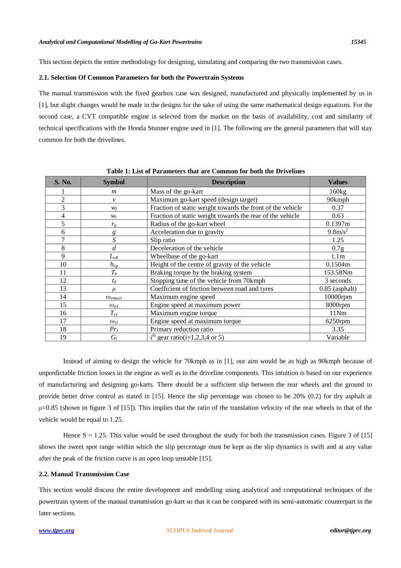
WrA is calculated as 1072.5N. This load WrA has been divided equally between the two rear wheels attached to the

rear axle.

Figure 1: Loading and Bending Moment Diagram of the Manual Transmission Rear Axle During Acceleration

In the above figure, the loading and the bending moment diagram of the rear axle is shown. The bearing and

plummer block reactions are computed as follows using moment balancing is Ra = 569.23N, Rb = 572.124N. Hence the

maximum bending moment MbA1 in the rear axle during acceleration is calculated as 67.032Nm.

Using the following bending stress equation [13], the selected dimensions of the shaft are checked for strength.

σbA1 = [15](4)

σbA1 is calculated as 48MPa. Since this value is much less than the yield strength (Syt) of the material, the rear axle

will not fail.

(ii)CASE-B1: Kart Deceleration

MtB1 is Maximum turning moment/torque on the rear axle during braking (provided by the brake disc). MtB1=Tb =

153.58Nm (Table 1). This would hence be the braking torque provided by the braking system of the go-kart, that acts in the

direction opposite to that of forward wheel motion. The dynamic weight shift on the rear axle during this deceleration from

a speed of 70kmph to rest would be computed as follows [21]:

WrB = [19](5)

WrB: Dynamic weight of the vehicle on the rear axle during braking/deceleration.

The parameters WrB and WrA have not been assigned the subscript 1 or 2 since both remain the same for manual

and CVT based transmission systems. WrB came out to be: 418.9N. The value of the above parameters has been mentioned

in Table 1. The load WrB would get equally divided amongst the two rear wheels of the vehicle.

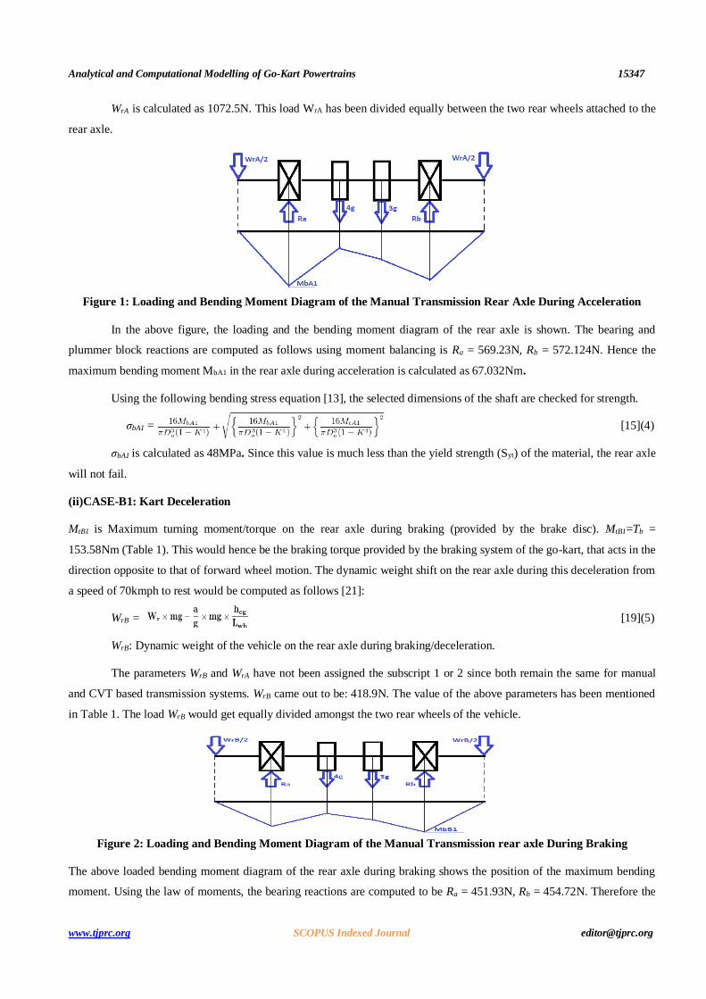
Figure 2: Loading and Bending Moment Diagram of the Manual Transmission rear axle During Braking

The above loaded bending moment diagram of the rear axle during braking shows the position of the maximum bending

moment. Using the law of moments, the bearing reactions are computed to be Ra = 451.93N, Rb = 454.72N. Therefore the



maximum bending moment on the rear axle during braking is calculated to be MbB1 = 52.46Nm. Using the following

bending stress equation [13], it would be decided whether the selected dimensions of the rear axle will undergo failure or

not.

σbB1 = [13] (6)

σbB1= 43.23MPa

Since this value is much below the yield strength of the material, the rear given rear axle will not fail under the

braking load conditions. Hence it can be concluded that the selected dimensions of the rear axle would sustain the given

loads.

2.2.4. Final Design of the Rear Axle

Since σbA1 > σbB1, we shall consider the acceleration case for computing the factor of safety of the design and during fatigue

analysis since it provides a higher bending stress on the rear axle.

FOS = Syt /σbA1 (7)

The factor of safety (FOS) of this shaft comes out to be 6.2, indicating that the final selected dimensions of the

shaft are safe from failure. Now the same value of FOS and K (ratio of inner to outer diameter) will be used for the rear

axle in Case-2 (CVT based driveline case), for the sake of proper comparison. The following CAD model of the manual

transmission case rear axle is developed along with proper keyways in NX-11.

Figure 3: CAD Model of the Manual Transmission Rear Axle Generated in NX-11

2.2.5. Validation by Fatigue Analysis using CAE

CAE using Ansys Workbench is performed on the rear axle to carry out fatigue analysis. Fatigue analysis was carried out

by varying the torque on the shaft in a sinusoidal manner, whereas the weights of the mounted components and that of the

vehicle load were made constant. The loads during vehicle acceleration were taken into account for fatigue calculations

since they generate a much higher bending stress on the rear axle. The aim of the analysis was to ensure that the design

would not fail under the given fatigue loading (i.e. FOS does not fall below 1.0). The moment on the rear axle would vary

in a sinusoidal manner as:

Te1*G1*Pr1*Sr1 – Te1*G5*Pr1*Sr1

Half cycle time would be the time taken for the moment to reach its minimum value from its maximum value, i.e.

time taken for the vehicle to accelerate from rest till maximum speed (90kmph). This is calculated in the subsequent

sections as slightly below 19 seconds. The following details were entered in the software, Moment: 153 – 51.64Nm

(Sinusoidal cycle), Half cycle time: 19 seconds. Additional vertical weights of mounted components and vehicle load WrA

are applied (as in the above loading and bending moment diagram of the acceleration case).Constraints: Cylindrical



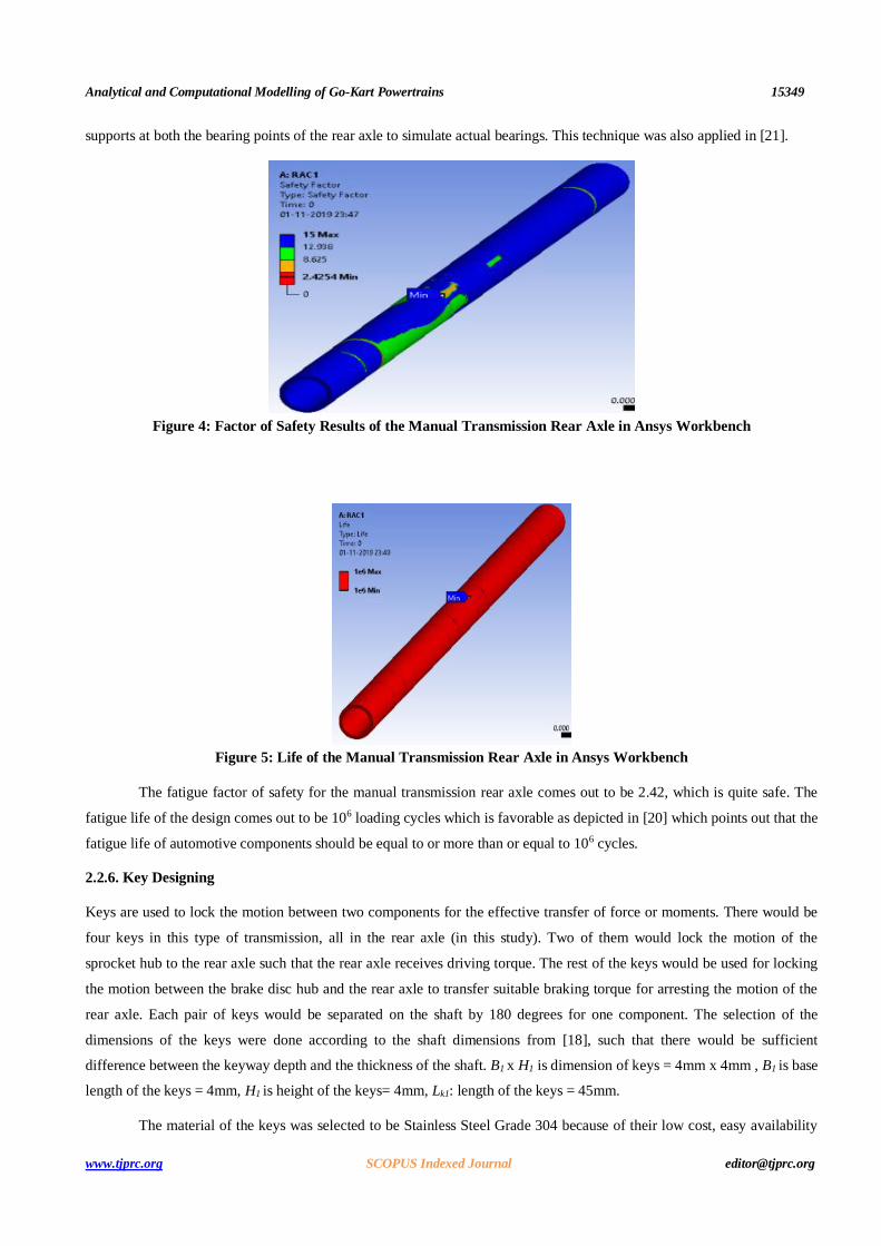
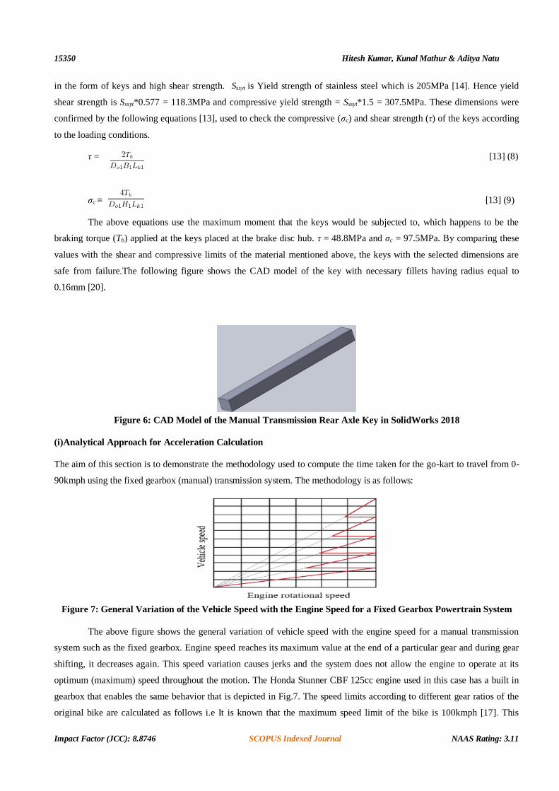
supports at both the bearing points of the rear axle to simulate actual bearings. This technique was also applied in [21].

Figure 4: Factor of Safety Results of the Manual Transmission Rear Axle in Ansys Workbench

Figure 5: Life of the Manual Transmission Rear Axle in Ansys Workbench

The fatigue factor of safety for the manual transmission rear axle comes out to be 2.42, which is quite safe. The

fatigue life of the design comes out to be 106 loading cycles which is favorable as depicted in [20] which points out that the

fatigue life of automotive components should be equal to or more than or equal to 106 cycles.

2.2.6. Key Designing

Keys are used to lock the motion between two components for the effective transfer of force or moments. There would be

four keys in this type of transmission, all in the rear axle (in this study). Two of them would lock the motion of the

sprocket hub to the rear axle such that the rear axle receives driving torque. The rest of the keys would be used for locking

the motion between the brake disc hub and the rear axle to transfer suitable braking torque for arresting the motion of the

rear axle. Each pair of keys would be separated on the shaft by 180 degrees for one component. The selection of the

dimensions of the keys were done according to the shaft dimensions from [18], such that there would be sufficient

difference between the keyway depth and the thickness of the shaft. B1 x H1 is dimension of keys = 4mm x 4mm , B1 is base

length of the keys = 4mm, H1 is height of the keys= 4mm, Lk1: length of the keys = 45mm.

The material of the keys was selected to be Stainless Steel Grade 304 because of their low cost, easy availability



in the form of keys and high shear strength. Sssyt is Yield strength of stainless steel which is 205MPa [14]. Hence yield

shear strength is Sssyt*0.577 = 118.3MPa and compressive yield strength = Sssyt*1.5 = 307.5MPa. These dimensions were

confirmed by the following equations [13], used to check the compressive (σc) and shear strength (τ) of the keys according

to the loading conditions.

τ = [13] (8)

σc = [13] (9)

The above equations use the maximum moment that the keys would be subjected to, which happens to be the

braking torque (Tb) applied at the keys placed at the brake disc hub. τ = 48.8MPa and σc = 97.5MPa. By comparing these

values with the shear and compressive limits of the material mentioned above, the keys with the selected dimensions are

safe from failure.The following figure shows the CAD model of the key with necessary fillets having radius equal to

0.16mm [20].

Figure 6: CAD Model of the Manual Transmission Rear Axle Key in SolidWorks 2018

(i)Analytical Approach for Acceleration Calculation

The aim of this section is to demonstrate the methodology used to compute the time taken for the go-kart to travel from 0-

90kmph using the fixed gearbox (manual) transmission system. The methodology is as follows:

Figure 7: General Variation of the Vehicle Speed with the Engine Speed for a Fixed Gearbox Powertrain System

The above figure shows the general variation of vehicle speed with the engine speed for a manual transmission

system such as the fixed gearbox. Engine speed reaches its maximum value at the end of a particular gear and during gear

shifting, it decreases again. This speed variation causes jerks and the system does not allow the engine to operate at its

optimum (maximum) speed throughout the motion. The Honda Stunner CBF 125cc engine used in this case has a built in

gearbox that enables the same behavior that is depicted in Fig.7. The speed limits according to different gear ratios of the

original bike are calculated as follows i.e It is known that the maximum speed limit of the bike is 100kmph [17]. This



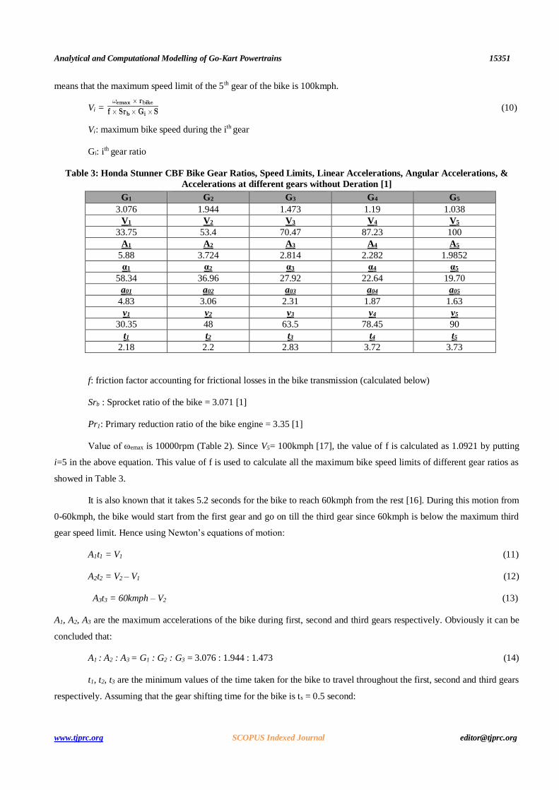
means that the maximum speed limit of the 5th gear of the bike is 100kmph.

Vi = (10)

Vi: maximum bike speed during the ith gear

Gi: ith gear ratio

Table 3: Honda Stunner CBF Bike Gear Ratios, Speed Limits, Linear Accelerations, Angular Accelerations, &

Accelerations at different gears without Deration [1]

G1 G2 G3 G4 G5

3.076 1.944 1.473 1.19 1.038

V1 V2 V3 V4 V5

33.75 53.4 70.47 87.23 100

A1 A2 A3 A4 A5

5.88 3.724 2.814 2.282 1.9852

α1 α2 α3 α4 α5

58.34 36.96 27.92 22.64 19.70

a01 a02 a03 a04 a05

4.83 3.06 2.31 1.87 1.63

v1 v2 v3 v4 v5

30.35 48 63.5 78.45 90

t1 t2 t3 t4 t5

2.18 2.2 2.83 3.72 3.73

f: friction factor accounting for frictional losses in the bike transmission (calculated below)

Srb : Sprocket ratio of the bike = 3.071 [1]

Pr1: Primary reduction ratio of the bike engine = 3.35 [1]

Value of ωemax is 10000rpm (Table 2). Since V5= 100kmph [17], the value of f is calculated as 1.0921 by putting

i=5 in the above equation. This value of f is used to calculate all the maximum bike speed limits of different gear ratios as

showed in Table 3.

It is also known that it takes 5.2 seconds for the bike to reach 60kmph from the rest [16]. During this motion from

0-60kmph, the bike would start from the first gear and go on till the third gear since 60kmph is below the maximum third

gear speed limit. Hence using Newton’s equations of motion:

A1t1 = V1 (11)

A2t2 = V2 – V1 (12)

A3t3 = 60kmph – V2 (13)

A1, A2, A3 are the maximum accelerations of the bike during first, second and third gears respectively. Obviously it can be

concluded that:

A1 : A2 : A3 = G1 : G2 : G3 = 3.076 : 1.944 : 1.473 (14)

t1, t2, t3 are the minimum values of the time taken for the bike to travel throughout the first, second and third gears

respectively. Assuming that the gear shifting time for the bike is ts = 0.5 second:



t1 + t2 + t3 = 5.2 – 2*ts (15)

Using the above five equations, the maximum linear accelerations for all the gears of the bike are as showed in

Table 3 as A1, A2..etc. Now let the angular accelerations of the gearbox outlet in the bike be denoted as αi where I = 1,2,3,4

or 5 for different gears.

αi= (16)

Hence the angular accelerations at the gearbox outlet shaft have been computed as showed in Table 3 as α.These angular

accelerations would be used to compute the linear acceleration values of the go-kart having the fixed gearbox as the

transmission driveline.

a0i = (17)

Where Sr1 was earlier computed as 1.35

Now we have the maximum acceleration values of the go-kart for each gear. By this logic, the speed limits for the

five gears of the go-kart can be calculated since the top speed is known as 90kmph (target for 70kmph). Variable vi is Top

speed of ith gear in the go-kart, v5 = 90 kmph. Since the ratios of all the vi are the same as inverse of the ratios of a0i, the

speed limits are calculated as showed in Table 3 as v. The go-kart also experiences rolling resistance which provides

resistance to motion. The coefficient of rolling resistance (Cr) is calculated as follows:

Cr = 0.05 + (1/b)*[0.01 + 0.0095(0.01*v)2] [8] (18)

ar=Crg (19)

Here b is the pressure of the rear tire in bar, v is the velocity in kmph and ar is the negative acceleration due to

rolling resistance. Since b = 20psi (past experience), the above equations can be simplified as:

ar = 0.562 + (6.75*10-6 * v2) (20)

Here v is in m/s. Now in order to calculate how much time is taken for the go-kart to travel from the rest to

90kmph, we will use the above obtained values. The actual accelerations during the different gears of the go-kart are

follows as, ai: Maximum actual linear acceleration of the go-kart for the ith gear

a1 = a01 – ar = 4.83 – [0.562 + (6.75x10-6 * v2)] (21)

a2 = a02 – ar = 3.06 - [0.562 + (6.75x10-6 * v2)] (22)

a3 = a03 – ar = 2.31 - [0.562 + (6.75x10-6 * v2)] (23)

a4 = a04 – ar = 1.87 - [0.562 + (6.75x10-6 * v2)] (24)

a5 = a05 – ar = 1.63 - [0.562 + (6.75x10-6 * v2)] (25)

Now in order to calculate how much time is taken for the go-kart to cover each and every gear with the lower and

the upper speed limits are known, the acceleration functions must be integrated between predefined limits since they are

continuous functions of velocities. During gear shifting in the go-kart, the engine is disconnected from the transmission due

to clutch disengagement. It is assumed that it takes 1 second for gear shifting in the go-kart [1]. Hence during these 1

second intervals, the speed of the go-kart must decrease due to the sole deceleration action of the acceleration due to rolling



resistance. Aerodynamic drag is neglected in the analytical part of the study due to the lower frontal area of the go-kart as

compared to other vehicles. Since the integration of continuous differential equations are involved, mathematical

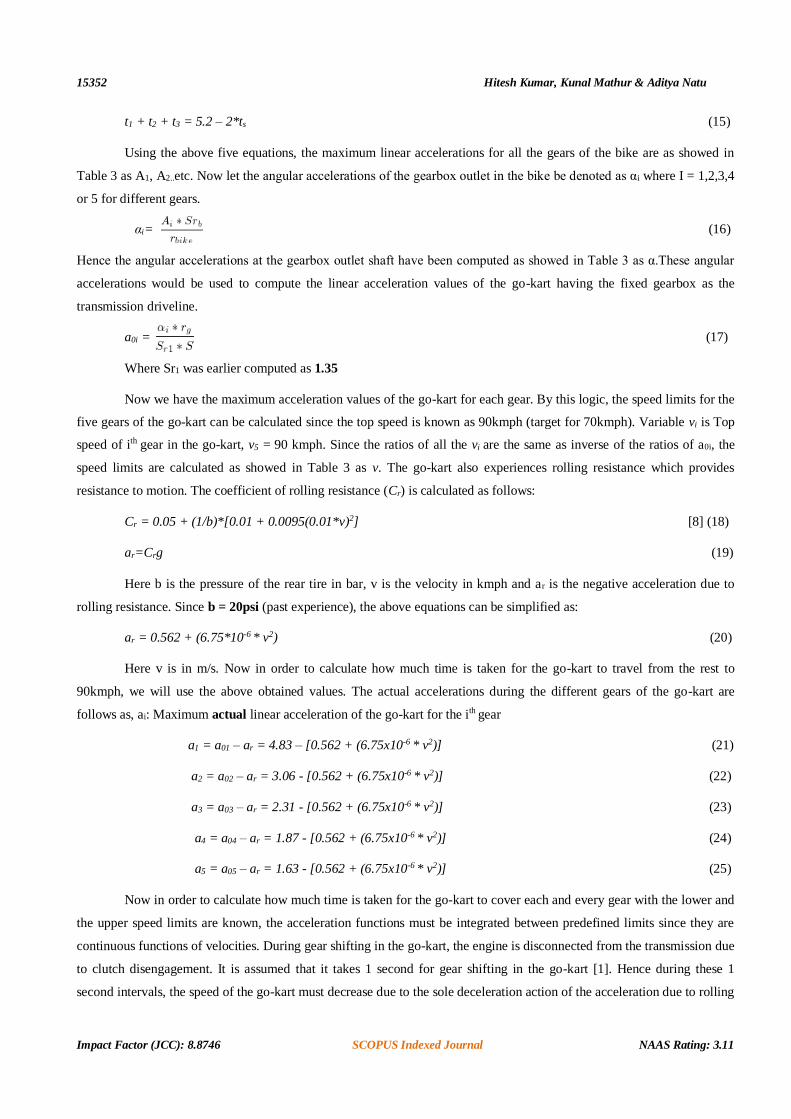
connections of MATLAB Simulink are used to solve the equations for obtaining the precise velocity variations with time.

Figure 8: MATLAB Simulink Model of Vehicle Speed Calculations for Different Gear Ratio

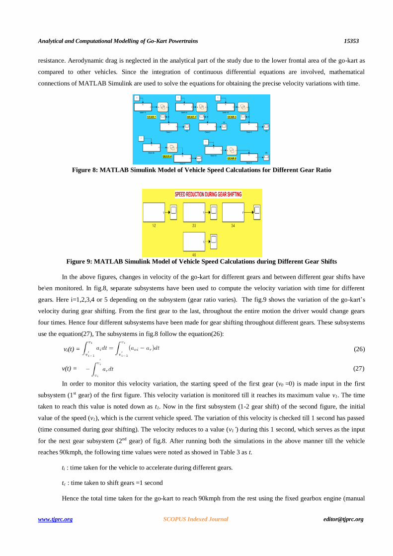
Figure 9: MATLAB Simulink Model of Vehicle Speed Calculations during Different Gear Shifts

In the above figures, changes in velocity of the go-kart for different gears and between different gear shifts have

be\en monitored. In fig.8, separate subsystems have been used to compute the velocity variation with time for different

gears. Here i=1,2,3,4 or 5 depending on the subsystem (gear ratio varies). The fig.9 shows the variation of the go-kart’s

velocity during gear shifting. From the first gear to the last, throughout the entire motion the driver would change gears

four times. Hence four different subsystems have been made for gear shifting throughout different gears. These subsystems

use the equation(27), The subsystems in fig.8 follow the equation(26):

vi(t) = (26)

v(t) = (27)

In order to monitor this velocity variation, the starting speed of the first gear (v0 =0) is made input in the first

subsystem (1st gear) of the first figure. This velocity variation is monitored till it reaches its maximum value v1. The time

taken to reach this value is noted down as t1. Now in the first subsystem (1-2 gear shift) of the second figure, the initial

value of the speed (v1), which is the current vehicle speed. The variation of this velocity is checked till 1 second has passed

(time consumed during gear shifting). The velocity reduces to a value (v1’) during this 1 second, which serves as the input

for the next gear subsystem (2nd gear) of fig.8. After running both the simulations in the above manner till the vehicle

reaches 90kmph, the following time values were noted as showed in Table 3 as t.

ti : time taken for the vehicle to accelerate during different gears.

tc : time taken to shift gears =1 second

Hence the total time taken for the go-kart to reach 90kmph from the rest using the fixed gearbox engine (manual



transmission) is computed as

(28)

= 18.66 seconds.

2.2.6. Computational Approach for Acceleration Calculation

Figure 10: MATLAB Simscape Model of the Manual Transmission go-kart powertrain

In this section, the entire physical model of the powertrain system was created in MATLAB Simscape. All the

standard mechanical components were selected from the Simscape Library and their respective parameters were made

input. All these components are connected using standard rotating elements simulating shafts. Apart from the parameters

included in the analytical section, this simulation also includes parameters such as stiffness and damping of each

component, drag factors like aerodynamic and rolling resistance, chain slack of sprocket, steady throttle input, clutch

actuation and slip, meshing losses in gears, etc. Hence this is a much more precise technique for simulating a powertrain

system and includes those parameters that could not be included in hand calculations. Moreover the clutch was introduced

in this model in order to smooth out the power flow from the engine to the vehicle body.

This simulation was run by changing the fixed gear ratio of the manual gearbox whenever the maximum kart

speed of a gear is achieved and disconnecting the clutch for 1 second while shifting the gears as done before. The total time

taken by the vehicle to reach 70kmph was computed as 19.4 seconds. The maximum speed limit was chosen to be 70kmph

instead of 90kmph because this simulation was expected to include all those real time parameters that were not present in

the analytical method. Since the computational result is similar to the corresponding result calculated by the analytical

approach, our safety margin of 90kmph is validated.

2.3 Semi-Automatic Transmission (CVT Case)

In this case, the powertrain components of the go-kart having the CVT would be designed, analyzed or selected. After

designing and selecting all the components, the powertrain would be modelled using analytical and computational

approaches. Most of the numerical values associated with this type of transmission system have been assigned the subscript

“2”.



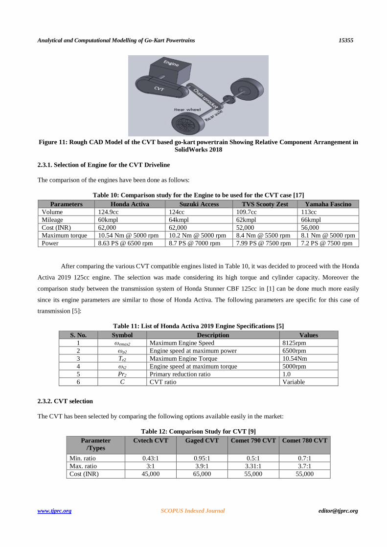
Figure 11: Rough CAD Model of the CVT based go-kart powertrain Showing Relative Component Arrangement in

SolidWorks 2018

2.3.1. Selection of Engine for the CVT Driveline

The comparison of the engines have been done as follows:

Table 10: Comparison study for the Engine to be used for the CVT case [17]

Parameters Honda Activa Suzuki Access TVS Scooty Zest Yamaha Fascino

Volume 124.9cc 124cc 109.7cc 113cc

Mileage 60kmpl 64kmpl 62kmpl 66kmpl

Cost (INR) 62,000 62,000 52,000 56,000

Maximum torque 10.54 Nm @ 5000 rpm 10.2 Nm @ 5000 rpm 8.4 Nm @ 5500 rpm 8.1 Nm @ 5000 rpm

Power 8.63 PS @ 6500 rpm 8.7 PS @ 7000 rpm 7.99 PS @ 7500 rpm 7.2 PS @ 7500 rpm

After comparing the various CVT compatible engines listed in Table 10, it was decided to proceed with the Honda

Activa 2019 125cc engine. The selection was made considering its high torque and cylinder capacity. Moreover the

comparison study between the transmission system of Honda Stunner CBF 125cc in [1] can be done much more easily

since its engine parameters are similar to those of Honda Activa. The following parameters are specific for this case of

transmission [5]:

Table 11: List of Honda Activa 2019 Engine Specifications [5]

S. No. Symbol Description Values

1 ωemax2 Maximum Engine Speed 8125rpm

2 ωp2 Engine speed at maximum power 6500rpm

3 Te2 Maximum Engine Torque 10.54Nm

4 ωt2 Engine speed at maximum torque 5000rpm

5 Pr2 Primary reduction ratio 1.0

6 C CVT ratio Variable

2.3.2. CVT selection

The CVT has been selected by comparing the following options available easily in the market:

Table 12: Comparison Study for CVT [9]

Parameter

/Types

Cvtech CVT Gaged CVT Comet 790 CVT Comet 780 CVT

Min. ratio 0.43:1 0.95:1 0.5:1 0.7:1

Max. ratio 3:1 3.9:1 3.31:1 3.7:1

Cost (INR) 45,000 65,000 55,000 55,000



A higher value of the ratio at minimum speed (Max. ratio) was required to provide a larger torque to propel the

vehicle. Moreover a higher value of the ratio at maximum speed (Min. ratio) was required to limit the actual maximum

vehicle speed to 90kmph. A high CVT ratio also allows a lower sprocket ratio since they decrease the size of the sprocket

connection. The Gaged GX9 CVT fits well within the desired ratio requirements. Apart from the above parameters, the

Gaged CVT is lighter, tune-able and is more reliable than the other CVTs [10]. Considering the above reasons, Gaged GX9

CVT was finally selected for the CVT based go-kart. Hence Cmax = 3.9; Cmin = 0.95.

2.3.3. Jackshaft Designing

(i)Design

The output from the CVT is transferred to the jackshaft which is directly attached to its outlet. The jackshaft houses the

smaller driver sprocket. Hence the jackshaft is driven by the CVT, which in turn drives the rear axle of the go-kart through

the chain sprocket assembly.

Material of the jackshaft was chosen to be AISI-1020 due to the reasons mentioned before. The following

specifications of the jackshaft were finalized after consulting with the technical experts of Gaged GX9 CVT sellers and

suppliers of AISI-1020 shafts: do2: Outer diameter of the jackshaft = 0.019m, di2: Inner diameter of the jackshaft = 0.0114m

(Providing weight optimization and allowing space for the keyways to be cut), b2 x h2: Dimensions of the key: (3/32)” x

(3/32)” (validated later), l2: Length of the jackshaft = 0.2m, k: ratio of inner to outer diameter = 0.6. The following

approach is used to confirm the above dimensions of the jackshaft, i.e. checking whether the jackshaft can handle the loads

subjected to it or not. Te2: Maximum engine torque = 10.54Nm (Table 11). Mt2: Maximum turning moment/torque on the

jackshaft, Mass of the CVT = 6.35kg [11]. Estimated mass of the driver sprocket with its keys, hub and fasteners = 2kg

Mt2 = Te2 * Cmax = 10.54*3.9 = 41.106Nm (29)

The mass of CVT on the jackshaft would be taken as 6.35kg itself, to model for the worst case scenario. The mass

of the smaller sprocket has been taken as higher than its actual mass to model for the worst.

Figure 12: Loading and Bending Moment Diagram of jackshaft (where g is the acceleration due to gravity).

The above figure shows the loaded bending moment diagram of the jackshaft where Mb2 is the maximum bending

moment. The CVT is attached at the left end of the shaft which provides bearing reaction Ra. The driver sprocket is

mounted at the midpoint of the jackshaft, followed by the bearing at the right most end providing reaction Rb. Mb2 was



calculated from moment balancing across the shaft as 0.981Nm.

σb2 = [13] (30)

The above equation [13] was used to ensure whether the bending stress, according to the selected dimensions of

the shaft was within the tensile yield strength or not. σb2 = 35.93 N/mm2

𝐹𝑂𝑆 = 𝑆𝑦𝑡 / 𝜎𝑏2 (31)

The factor of safety FOS comes out to be 8.2 which is quite safe.

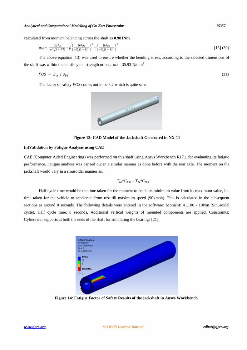
Figure 13: CAD Model of the Jackshaft Generated in NX-11

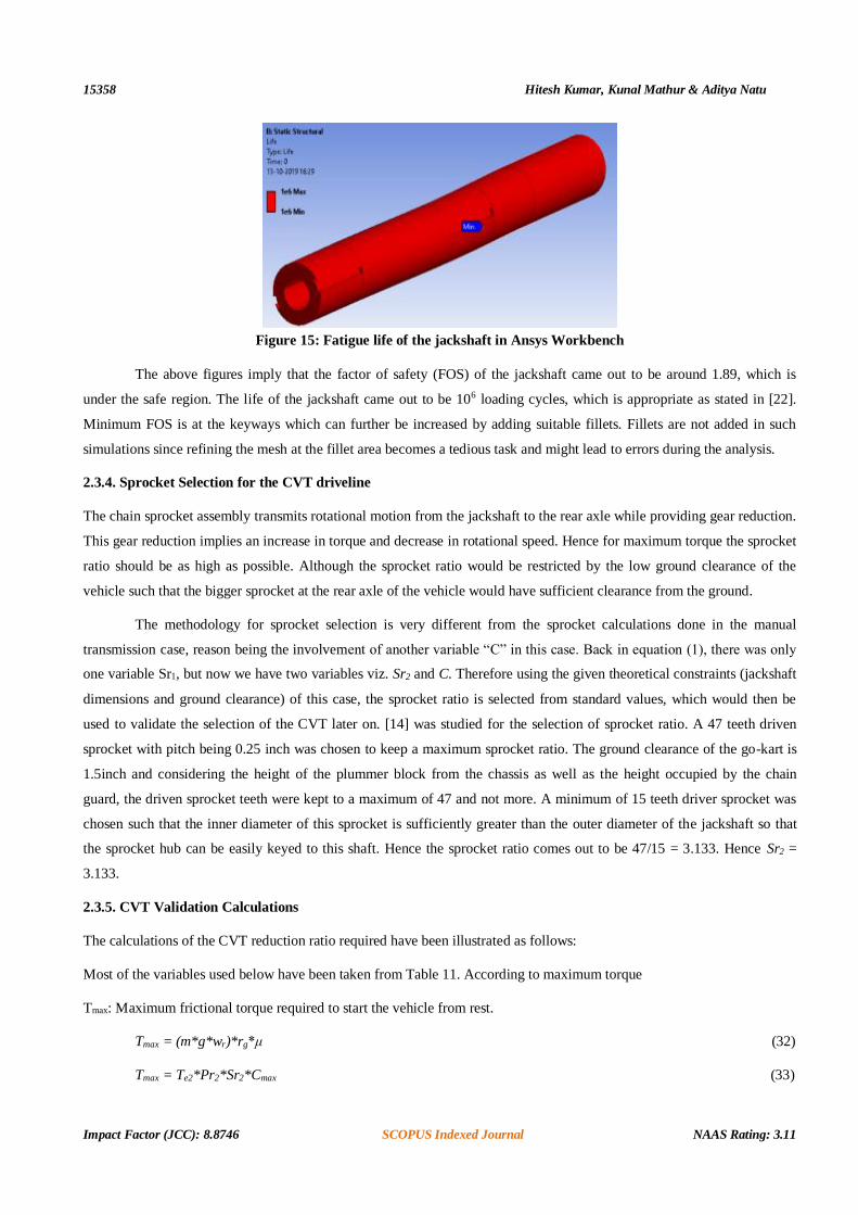
(ii)Validation by Fatigue Analysis using CAE

CAE (Computer Aided Engineering) was performed on this shaft using Ansys Workbench R17.1 for evaluating its fatigue

performance. Fatigue analysis was carried out in a similar manner as done before with the rear axle. The moment on the

jackshaft would vary in a sinusoidal manner as:

Te2*Cmax – Te2*Cmin

Half cycle time would be the time taken for the moment to reach its minimum value from its maximum value, i.e.

time taken for the vehicle to accelerate from rest till maximum speed (90kmph). This is calculated in the subsequent

sections as around 8 seconds. The following details were entered in the software: Moment: 41.106 - 10Nm (Sinusoidal

cycle), Half cycle time: 8 seconds, Additional vertical weights of mounted components are applied, Constraints:

Cylindrical supports at both the ends of the shaft for simulating the bearings [21].

Figure 14: Fatigue Factor of Safety Results of the jackshaft in Ansys Workbench.



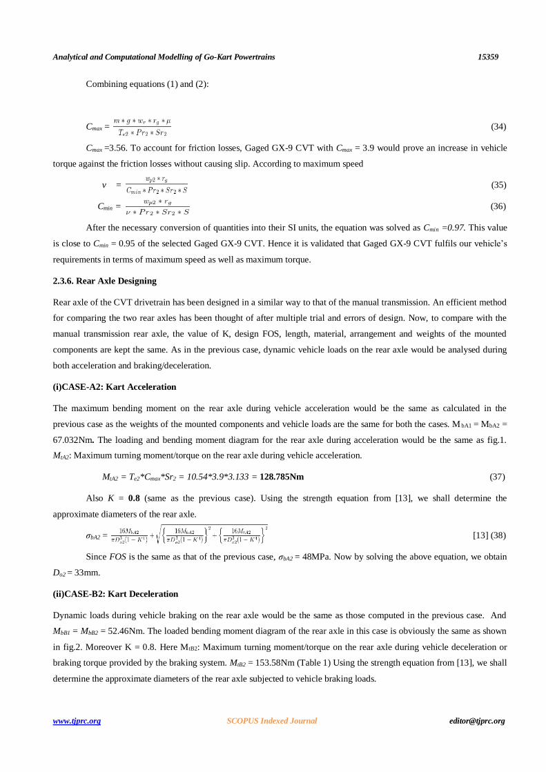
Figure 15: Fatigue life of the jackshaft in Ansys Workbench

The above figures imply that the factor of safety (FOS) of the jackshaft came out to be around 1.89, which is

under the safe region. The life of the jackshaft came out to be 106 loading cycles, which is appropriate as stated in [22].

Minimum FOS is at the keyways which can further be increased by adding suitable fillets. Fillets are not added in such

simulations since refining the mesh at the fillet area becomes a tedious task and might lead to errors during the analysis.

2.3.4. Sprocket Selection for the CVT driveline

The chain sprocket assembly transmits rotational motion from the jackshaft to the rear axle while providing gear reduction.

This gear reduction implies an increase in torque and decrease in rotational speed. Hence for maximum torque the sprocket

ratio should be as high as possible. Although the sprocket ratio would be restricted by the low ground clearance of the

vehicle such that the bigger sprocket at the rear axle of the vehicle would have sufficient clearance from the ground.

The methodology for sprocket selection is very different from the sprocket calculations done in the manual

transmission case, reason being the involvement of another variable “C” in this case. Back in equation (1), there was only

one variable Sr1, but now we have two variables viz. Sr2 and C. Therefore using the given theoretical constraints (jackshaft

dimensions and ground clearance) of this case, the sprocket ratio is selected from standard values, which would then be

used to validate the selection of the CVT later on. [14] was studied for the selection of sprocket ratio. A 47 teeth driven

sprocket with pitch being 0.25 inch was chosen to keep a maximum sprocket ratio. The ground clearance of the go-kart is

1.5inch and considering the height of the plummer block from the chassis as well as the height occupied by the chain

guard, the driven sprocket teeth were kept to a maximum of 47 and not more. A minimum of 15 teeth driver sprocket was

chosen such that the inner diameter of this sprocket is sufficiently greater than the outer diameter of the jackshaft so that

the sprocket hub can be easily keyed to this shaft. Hence the sprocket ratio comes out to be 47/15 = 3.133. Hence Sr2 =

3.133.

2.3.5. CVT Validation Calculations

The calculations of the CVT reduction ratio required have been illustrated as follows:

Most of the variables used below have been taken from Table 11. According to maximum torque

Tmax: Maximum frictional torque required to start the vehicle from rest.

Tmax = (m*g*wr)*rg*μ (32)

Tmax = Te2*Pr2*Sr2*Cmax (33)



Combining equations (1) and (2):

Cmax = (34)

Cmax =3.56. To account for friction losses, Gaged GX-9 CVT with Cmax = 3.9 would prove an increase in vehicle

torque against the friction losses without causing slip. According to maximum speed

v = (35)

Cmin = (36)

After the necessary conversion of quantities into their SI units, the equation was solved as Cmin =0.97. This value

is close to Cmin = 0.95 of the selected Gaged GX-9 CVT. Hence it is validated that Gaged GX-9 CVT fulfils our vehicle’s

requirements in terms of maximum speed as well as maximum torque.

2.3.6. Rear Axle Designing

Rear axle of the CVT drivetrain has been designed in a similar way to that of the manual transmission. An efficient method

for comparing the two rear axles has been thought of after multiple trial and errors of design. Now, to compare with the

manual transmission rear axle, the value of K, design FOS, length, material, arrangement and weights of the mounted

components are kept the same. As in the previous case, dynamic vehicle loads on the rear axle would be analysed during

both acceleration and braking/deceleration.

(i)CASE-A2: Kart Acceleration

The maximum bending moment on the rear axle during vehicle acceleration would be the same as calculated in the

previous case as the weights of the mounted components and vehicle loads are the same for both the cases. M bA1 = MbA2 =

67.032Nm. The loading and bending moment diagram for the rear axle during acceleration would be the same as fig.1.

MtA2: Maximum turning moment/torque on the rear axle during vehicle acceleration.

MtA2 = Te2*Cmax*Sr2 = 10.54*3.9*3.133 = 128.785Nm (37)

Also K = 0.8 (same as the previous case). Using the strength equation from [13], we shall determine the

approximate diameters of the rear axle.

σbA2 = [13] (38)

Since FOS is the same as that of the previous case, σbA2 = 48MPa. Now by solving the above equation, we obtain

Do2 = 33mm.

(ii)CASE-B2: Kart Deceleration

Dynamic loads during vehicle braking on the rear axle would be the same as those computed in the previous case. And

MbB1 = MbB2 = 52.46Nm. The loaded bending moment diagram of the rear axle in this case is obviously the same as shown

in fig.2. Moreover K = 0.8. Here MtB2: Maximum turning moment/torque on the rear axle during vehicle deceleration or

braking torque provided by the braking system. MtB2 = 153.58Nm (Table 1) Using the strength equation from [13], we shall

determine the approximate diameters of the rear axle subjected to vehicle braking loads.



σbA2 = [13] (39)

Since the FOS was to be constant, σbA2 = 48MPa, as in the previous transmission case. By solving the above

equation, we obtain Do2 = 33.5mm.

(iii)Final Design of the Rear Axle

Now, comparing the acceleration and the braking case, the diameter in the braking case comes out to be the largest. Hence

the braking event of the vehicle would generate the largest load on the rear axle, in contrast to what happened in the

manual transmission case where the acceleration load was the largest. Now this braking event would be used in the fatigue

analysis of the rear axle to make the design safer against the high braking loads.

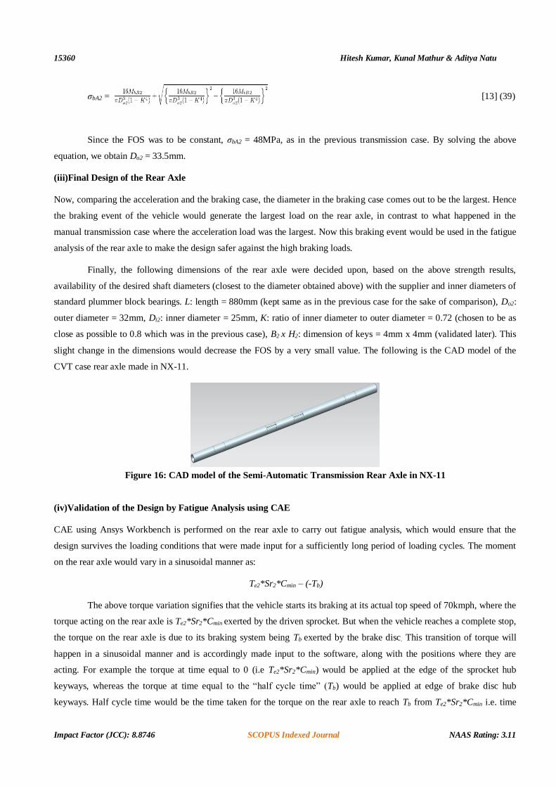
Finally, the following dimensions of the rear axle were decided upon, based on the above strength results,

availability of the desired shaft diameters (closest to the diameter obtained above) with the supplier and inner diameters of

standard plummer block bearings. L: length = 880mm (kept same as in the previous case for the sake of comparison), Do2:

outer diameter = 32mm, Di2: inner diameter = 25mm, K: ratio of inner diameter to outer diameter = 0.72 (chosen to be as

close as possible to 0.8 which was in the previous case), B2 x H2: dimension of keys = 4mm x 4mm (validated later). This

slight change in the dimensions would decrease the FOS by a very small value. The following is the CAD model of the

CVT case rear axle made in NX-11.

Figure 16: CAD model of the Semi-Automatic Transmission Rear Axle in NX-11

(iv)Validation of the Design by Fatigue Analysis using CAE

CAE using Ansys Workbench is performed on the rear axle to carry out fatigue analysis, which would ensure that the

design survives the loading conditions that were made input for a sufficiently long period of loading cycles. The moment

on the rear axle would vary in a sinusoidal manner as:

Te2*Sr2*Cmin – (-Tb)

The above torque variation signifies that the vehicle starts its braking at its actual top speed of 70kmph, where the

torque acting on the rear axle is Te2*Sr2*Cmin exerted by the driven sprocket. But when the vehicle reaches a complete stop,

the torque on the rear axle is due to its braking system being Tb exerted by the brake disc. This transition of torque will

happen in a sinusoidal manner and is accordingly made input to the software, along with the positions where they are

acting. For example the torque at time equal to 0 (i.e Te2*Sr2*Cmin) would be applied at the edge of the sprocket hub

keyways, whereas the torque at time equal to the “half cycle time” (Tb) would be applied at edge of brake disc hub

keyways. Half cycle time would be the time taken for the torque on the rear axle to reach Tb from Te2*Sr2*Cmin i.e. time



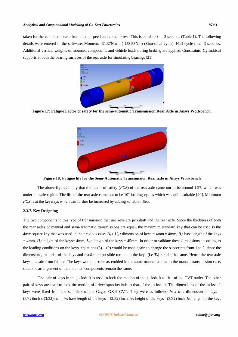
taken for the vehicle to brake from its top speed and come to rest. This is equal to td = 3 seconds (Table 1). The following

details were entered in the software: Moment: 31.37Nm – (-153.58Nm) (Sinusoidal cycle), Half cycle time: 3 seconds.

Additional vertical weights of mounted components and vehicle loads during braking are applied. Constraints: Cylindrical

supports at both the bearing surfaces of the rear axle for simulating bearings [21].

Figure 17: Fatigue Factor of safety for the semi-automatic Transmission Rear Axle in Ansys Workbench.

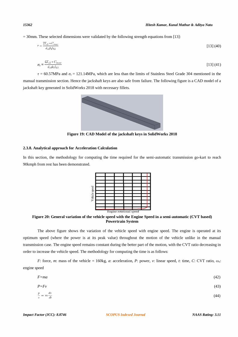
Figure 18: Fatigue life for the Semi-Automatic Transmission Rear axle in Ansys Workbench

The above figures imply that the factor of safety (FOS) of the rear axle came out to be around 1.27, which was

under the safe region. The life of the rear axle came out to be 106 loading cycles which was quite suitable [20]. Minimum

FOS is at the keyways which can further be increased by adding suitable fillets.

2.3.7. Key Designing

The two components in this type of transmission that use keys are jackshaft and the rear axle. Since the thickness of both

the rear axles of manual and semi-automatic transmissions are equal, the maximum standard key that can be used is the

4mm square key that was used in the previous case. B2 x H2 : dimension of keys = 4mm x 4mm, B2: base length of the keys

= 4mm, H2: height of the keys= 4mm, Lk2: length of the keys = 45mm. In order to validate these dimensions according to

the loading conditions on the keys, equations (8) – (9) would be used again to change the subscripts from 1 to 2, since the

dimensions, material of the keys and maximum possible torque on the keys (i.e Tb) remain the same. Hence the rear axle

keys are safe from failure. The keys would also be assembled in the same manner as that in the manual transmission case,

since the arrangement of the mounted components remain the same.

One pair of keys in the jackshaft is used to lock the motion of the jackshaft to that of the CVT outlet. The other

pair of keys are used to lock the motion of driver sprocket hub to that of the jackshaft. The dimensions of the jackshaft

keys were fixed from the suppliers of the Gaged GX-9 CVT. They were as follows: b2 x h2 : dimension of keys =

(3/32)inch x (3/32)inch , b2: base length of the keys = (3/32) inch, h2: height of the keys= (3/32) inch ,lk2: length of the keys



= 30mm. These selected dimensions were validated by the following strength equations from [13]:

[13] (40)

σc = [13] (41)

τ = 60.57MPa and σc = 121.14MPa, which are less than the limits of Stainless Steel Grade 304 mentioned in the

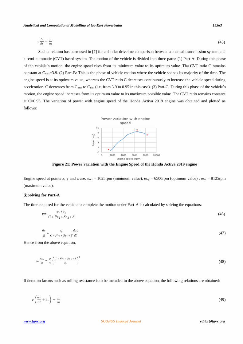
manual transmission section. Hence the jackshaft keys are also safe from failure. The following figure is a CAD model of a

jackshaft key generated in SolidWorks 2018 with necessary fillets.

Figure 19: CAD Model of the jackshaft keys in SolidWorks 2018

2.3.8. Analytical approach for Acceleration Calculation

In this section, the methodology for computing the time required for the semi-automatic transmission go-kart to reach

90kmph from rest has been demonstrated.

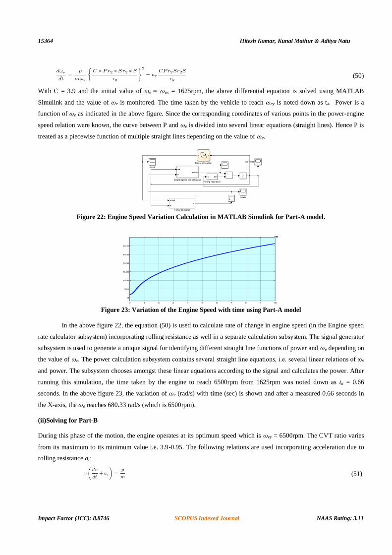
Figure 20: General variation of the vehicle speed with the Engine Speed in a semi-automatic (CVT based)

Powertrain System

The above figure shows the variation of the vehicle speed with engine speed. The engine is operated at its

optimum speed (where the power is at its peak value) throughout the motion of the vehicle unlike in the manual

transmission case. The engine speed remains constant during the better part of the motion, with the CVT ratio decreasing in

order to increase the vehicle speed. The methodology for computing the time is as follows:

F: force, m: mass of the vehicle = 160kg, a: acceleration, P: power, v: linear speed, t: time, C: CVT ratio, ωe:

engine speed

F=ma (42)

P=Fv (43)

(44)



(45)

Such a relation has been used in [7] for a similar driveline comparison between a manual transmission system and

a semi-automatic (CVT) based system. The motion of the vehicle is divided into three parts: (1) Part-A: During this phase

of the vehicle’s motion, the engine speed rises from its minimum value to its optimum value. The CVT ratio C remains

constant at Cmax=3.9. (2) Part-B: This is the phase of vehicle motion where the vehicle spends its majority of the time. The

engine speed is at its optimum value, whereas the CVT ratio C decreases continuously to increase the vehicle speed during

acceleration. C decreases from Cmax to Cmin (i.e. from 3.9 to 0.95 in this case). (3) Part-C: During this phase of the vehicle’s

motion, the engine speed increases from its optimum value to its maximum possible value. The CVT ratio remains constant

at C=0.95. The variation of power with engine speed of the Honda Activa 2019 engine was obtained and plotted as

follows:

Figure 21: Power variation with the Engine Speed of the Honda Activa 2019 engine

Engine speed at points x, y and z are: ωex = 1625rpm (minimum value), ωey = 6500rpm (optimum value) , ωez = 8125rpm

(maximum value).

(i)Solving for Part-A

The time required for the vehicle to complete the motion under Part-A is calculated by solving the equations:

v= (46)

(47)

Hence from the above equation,

(48)

If deration factors such as rolling resistance is to be included in the above equation, the following relations are obtained:

(49)



(50)

With C = 3.9 and the initial value of ωe = ωex = 1625rpm, the above differential equation is solved using MATLAB

Simulink and the value of ωe is monitored. The time taken by the vehicle to reach ωey is noted down as ta. Power is a

function of ωe as indicated in the above figure. Since the corresponding coordinates of various points in the power-engine

speed relation were known, the curve between P and ωe is divided into several linear equations (straight lines). Hence P is

treated as a piecewise function of multiple straight lines depending on the value of ωe.

Figure 22: Engine Speed Variation Calculation in MATLAB Simulink for Part-A model.

Figure 23: Variation of the Engine Speed with time using Part-A model

In the above figure 22, the equation (50) is used to calculate rate of change in engine speed (in the Engine speed

rate calculator subsystem) incorporating rolling resistance as well in a separate calculation subsystem. The signal generator

subsystem is used to generate a unique signal for identifying different straight line functions of power and ωe depending on

the value of ωe. The power calculation subsystem contains several straight line equations, i.e. several linear relations of ωe

and power. The subsystem chooses amongst these linear equations according to the signal and calculates the power. After

running this simulation, the time taken by the engine to reach 6500rpm from 1625rpm was noted down as ta = 0.66

seconds. In the above figure 23, the variation of ωe (rad/s) with time (sec) is shown and after a measured 0.66 seconds in

the X-axis, the ωe reaches 680.33 rad/s (which is 6500rpm).

(ii)Solving for Part-B

During this phase of the motion, the engine operates at its optimum speed which is ωey = 6500rpm. The CVT ratio varies

from its maximum to its minimum value i.e. 3.9-0.95. The following relations are used incorporating acceleration due to

rolling resistance ar:

(51)



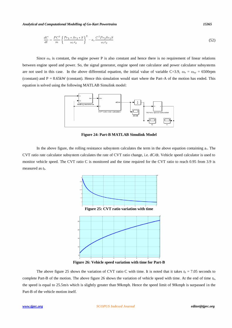
(52)

Since ωe is constant, the engine power P is also constant and hence there is no requirement of linear relations

between engine speed and power. So, the signal generator, engine speed rate calculator and power calculator subsystems

are not used in this case. In the above differential equation, the initial value of variable C=3.9, ωe = ωey = 6500rpm

(constant) and P = 8.65kW (constant). Hence this simulation would start where the Part-A of the motion has ended. This

equation is solved using the following MATLAB Simulink model:

Figure 24: Part-B MATLAB Simulink Model

In the above figure, the rolling resistance subsystem calculates the term in the above equation containing a r. The

CVT ratio rate calculator subsystem calculates the rate of CVT ratio change, i.e. dC/dt. Vehicle speed calculator is used to

monitor vehicle speed. The CVT ratio C is monitored and the time required for the CVT ratio to reach 0.95 from 3.9 is

measured as tb.

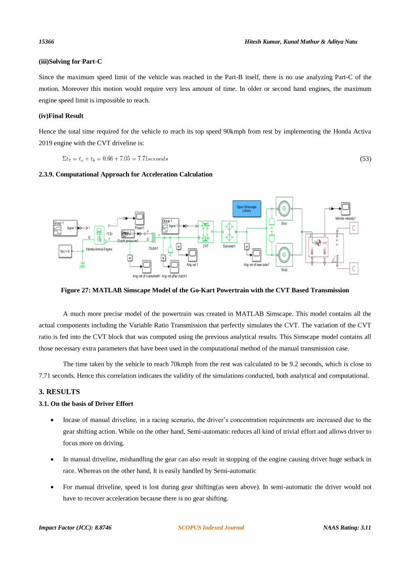
Figure 25: CVT ratio variation with time

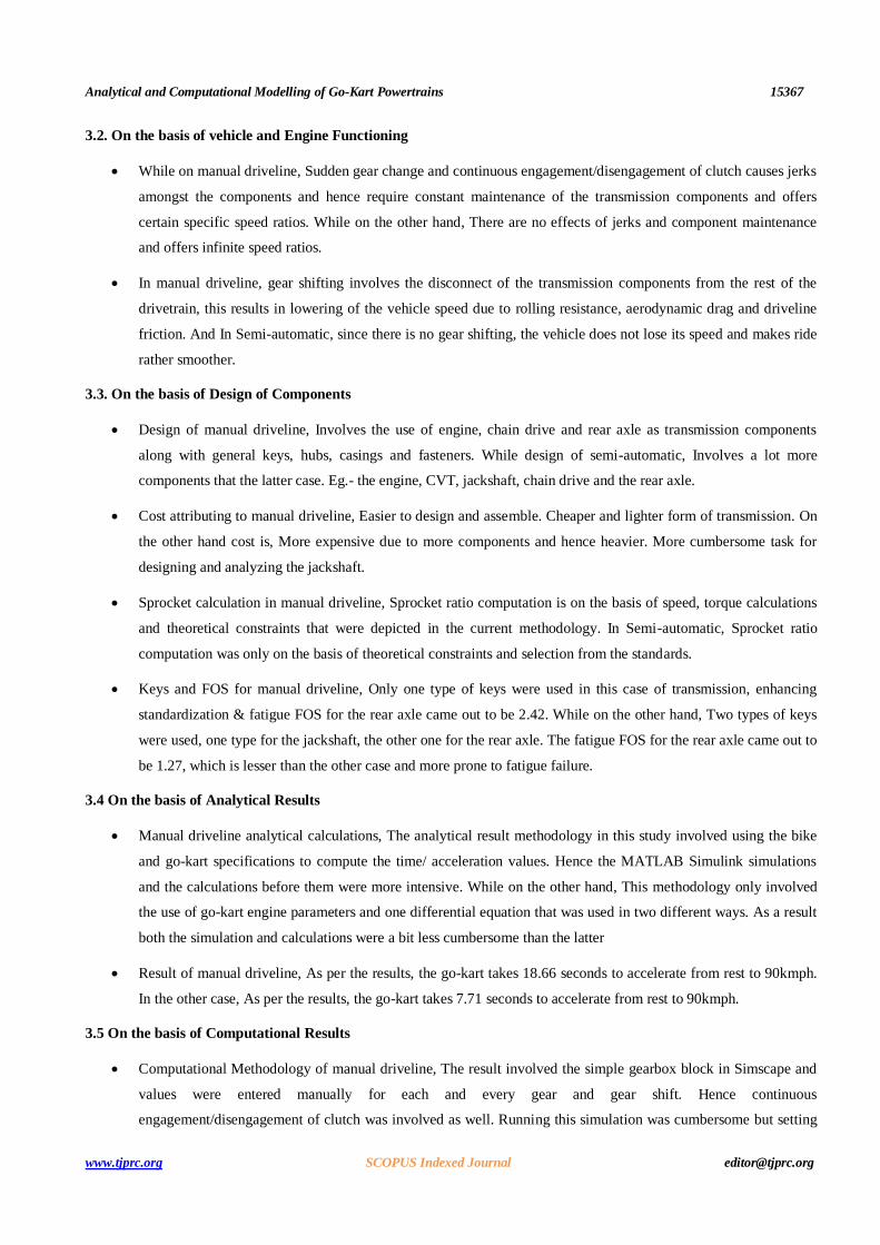
Figure 26: Vehicle speed variation with time for Part-B

The above figure 25 shows the variation of CVT ratio C with time. It is noted that it takes tb = 7.05 seconds to

complete Part-B of the motion. The above figure 26 shows the variation of vehicle speed with time. At the end of time tb,

the speed is equal to 25.5m/s which is slightly greater than 90kmph. Hence the speed limit of 90kmph is surpassed in the

Part-B of the vehicle motion itself.



(iii)Solving for Part-C

Since the maximum speed limit of the vehicle was reached in the Part-B itself, there is no use analyzing Part-C of the

motion. Moreover this motion would require very less amount of time. In older or second hand engines, the maximum

engine speed limit is impossible to reach.

(iv)Final Result

Hence the total time required for the vehicle to reach its top speed 90kmph from rest by implementing the Honda Activa

2019 engine with the CVT driveline is:

(53)

2.3.9. Computational Approach for Acceleration Calculation

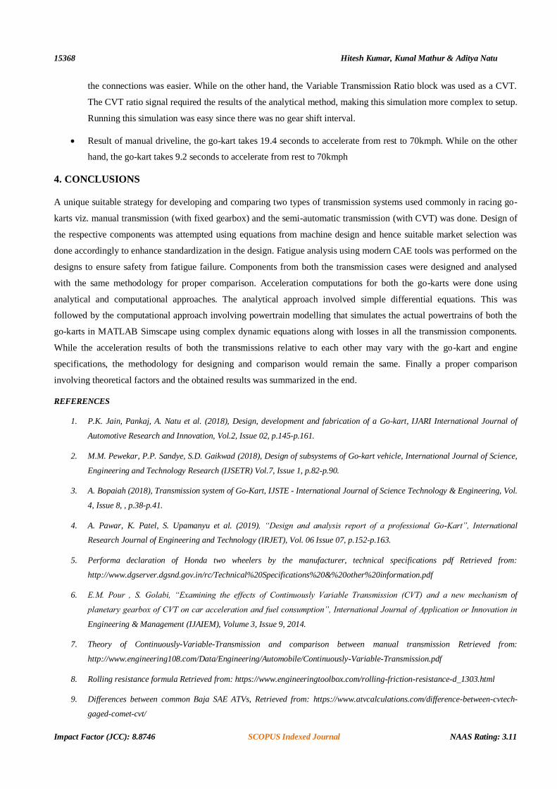
Figure 27: MATLAB Simscape Model of the Go-Kart Powertrain with the CVT Based Transmission

A much more precise model of the powertrain was created in MATLAB Simscape. This model contains all the

actual components including the Variable Ratio Transmission that perfectly simulates the CVT. The variation of the CVT

ratio is fed into the CVT block that was computed using the previous analytical results. This Simscape model contains all

those necessary extra parameters that have been used in the computational method of the manual transmission case.

The time taken by the vehicle to reach 70kmph from the rest was calculated to be 9.2 seconds, which is close to

7.71 seconds. Hence this correlation indicates the validity of the simulations conducted, both analytical and computational.

3. RESULTS

3.1. On the basis of Driver Effort

Incase of manual driveline, in a racing scenario, the driver’s concentration requirements are increased due to the

gear shifting action. While on the other hand, Semi-automatic reduces all kind of trivial effort and allows driver to

focus more on driving.

In manual driveline, mishandling the gear can also result in stopping of the engine causing driver huge setback in

race. Whereas on the other hand, It is easily handled by Semi-automatic

For manual driveline, speed is lost during gear shifting(as seen above). In semi-automatic the driver would not

have to recover acceleration because there is no gear shifting.



3.2. On the basis of vehicle and Engine Functioning

While on manual driveline, Sudden gear change and continuous engagement/disengagement of clutch causes jerks

amongst the components and hence require constant maintenance of the transmission components and offers

certain specific speed ratios. While on the other hand, There are no effects of jerks and component maintenance

and offers infinite speed ratios.

In manual driveline, gear shifting involves the disconnect of the transmission components from the rest of the

drivetrain, this results in lowering of the vehicle speed due to rolling resistance, aerodynamic drag and driveline

friction. And In Semi-automatic, since there is no gear shifting, the vehicle does not lose its speed and makes ride

rather smoother.

3.3. On the basis of Design of Components

Design of manual driveline, Involves the use of engine, chain drive and rear axle as transmission components

along with general keys, hubs, casings and fasteners. While design of semi-automatic, Involves a lot more

components that the latter case. Eg.- the engine, CVT, jackshaft, chain drive and the rear axle.

Cost attributing to manual driveline, Easier to design and assemble. Cheaper and lighter form of transmission. On

the other hand cost is, More expensive due to more components and hence heavier. More cumbersome task for

designing and analyzing the jackshaft.

Sprocket calculation in manual driveline, Sprocket ratio computation is on the basis of speed, torque calculations

and theoretical constraints that were depicted in the current methodology. In Semi-automatic, Sprocket ratio

computation was only on the basis of theoretical constraints and selection from the standards.

Keys and FOS for manual driveline, Only one type of keys were used in this case of transmission, enhancing

standardization & fatigue FOS for the rear axle came out to be 2.42. While on the other hand, Two types of keys

were used, one type for the jackshaft, the other one for the rear axle. The fatigue FOS for the rear axle came out to

be 1.27, which is lesser than the other case and more prone to fatigue failure.

3.4 On the basis of Analytical Results

Manual driveline analytical calculations, The analytical result methodology in this study involved using the bike

and go-kart specifications to compute the time/ acceleration values. Hence the MATLAB Simulink simulations

and the calculations before them were more intensive. While on the other hand, This methodology only involved

the use of go-kart engine parameters and one differential equation that was used in two different ways. As a result

both the simulation and calculations were a bit less cumbersome than the latter

Result of manual driveline, As per the results, the go-kart takes 18.66 seconds to accelerate from rest to 90kmph.

In the other case, As per the results, the go-kart takes 7.71 seconds to accelerate from rest to 90kmph.

3.5 On the basis of Computational Results

Computational Methodology of manual driveline, The result involved the simple gearbox block in Simscape and

values were entered manually for each and every gear and gear shift. Hence continuous

engagement/disengagement of clutch was involved as well. Running this simulation was cumbersome but setting



the connections was easier. While on the other hand, the Variable Transmission Ratio block was used as a CVT.

The CVT ratio signal required the results of the analytical method, making this simulation more complex to setup.

Running this simulation was easy since there was no gear shift interval.

Result of manual driveline, the go-kart takes 19.4 seconds to accelerate from rest to 70kmph. While on the other

hand, the go-kart takes 9.2 seconds to accelerate from rest to 70kmph

4. CONCLUSIONS

A unique suitable strategy for developing and comparing two types of transmission systems used commonly in racing go-

karts viz. manual transmission (with fixed gearbox) and the semi-automatic transmission (with CVT) was done. Design of

the respective components was attempted using equations from machine design and hence suitable market selection was

done accordingly to enhance standardization in the design. Fatigue analysis using modern CAE tools was performed on the

designs to ensure safety from fatigue failure. Components from both the transmission cases were designed and analysed

with the same methodology for proper comparison. Acceleration computations for both the go-karts were done using

analytical and computational approaches. The analytical approach involved simple differential equations. This was

followed by the computational approach involving powertrain modelling that simulates the actual powertrains of both the

go-karts in MATLAB Simscape using complex dynamic equations along with losses in all the transmission components.

While the acceleration results of both the transmissions relative to each other may vary with the go-kart and engine

specifications, the methodology for designing and comparison would remain the same. Finally a proper comparison

involving theoretical factors and the obtained results was summarized in the end.

REFERENCES

1. P.K. Jain, Pankaj, A. Natu et al. (2018), Design, development and fabrication of a Go-kart, IJARI International Journal of

Automotive Research and Innovation, Vol.2, Issue 02, p.145-p.161.

2. M.M. Pewekar, P.P. Sandye, S.D. Gaikwad (2018), Design of subsystems of Go-kart vehicle, International Journal of Science,

Engineering and Technology Research (IJSETR) Vol.7, Issue 1, p.82-p.90.

3. A. Bopaiah (2018), Transmission system of Go-Kart, IJSTE - International Journal of Science Technology & Engineering, Vol.

4, Issue 8, , p.38-p.41.

4. A. Pawar, K. Patel, S. Upamanyu et al. (2019), “Design and analysis report of a professional Go-Kart”, International

Research Journal of Engineering and Technology (IRJET), Vol. 06 Issue 07, p.152-p.163.

5. Performa declaration of Honda two wheelers by the manufacturer, technical specifications pdf Retrieved from:

http://www.dgserver.dgsnd.gov.in/rc/Technical%20Specifications%20&%20other%20information.pdf

6. E.M. Pour , S. Golabi, “Examining the effects of Continuously Variable Transmission (CVT) and a new mechanism of

planetary gearbox of CVT on car acceleration and fuel consumption”, International Journal of Application or Innovation in

Engineering & Management (IJAIEM), Volume 3, Issue 9, 2014.

7. Theory of Continuously-Variable-Transmission and comparison between manual transmission Retrieved from:

http://www.engineering108.com/Data/Engineering/Automobile/Continuously-Variable-Transmission.pdf

8. Rolling resistance formula Retrieved from: https://www.engineeringtoolbox.com/rolling-friction-resistance-d_1303.html

9. Differences between common Baja SAE ATVs, Retrieved from: https://www.atvcalculations.com/difference-between-cvtech-

gaged-comet-cvt/

http://www.dgserver.dgsnd.gov.in/rc/Technical%20Specifications%20&%20other%20information.pdf

http://www.engineering108.com/Data/Engineering/Automobile/Continuously-Variable-Transmission.pdf

https://www.atvcalculations.com/difference-between-cvtech-gaged-comet-cvt/

https://www.atvcalculations.com/difference-between-cvtech-gaged-comet-cvt/



10. K. Piepmeyer, “A baccalaureate thesis” submitted to the Department of Mechanical and Materials Engineering College of

Engineering and Applied Science University of Cincinnati, 2016 University of Cincinnati Baja SAE Drivetrain.

11. E.T. Garza, “2016-2017 drivetrain overview”, October 30, 2016, Ur Baja Sae Yellow Jacket Racing Retrieved from,

https://sa.rochester.edu/baja/2016/10/2016-

2017drivetrainoverview/#targetText=The%20Gaged%20CVT%20itself%20weighs,ratio%2C%20meaning%20a%20lighter%2

0gearbox.

12. Azom.com for material properties Retrieved from https://www.azom.com/article. aspx?ArticleID=6114

13. V.B. Bhandari. Design of Machine Elements. Third Edition, p.333.

14. Brewton Iron Works Inc., Sprocket Engineering Data Retrieved from, https://dokumen.tips/documents/sprocket-engineering-

data-brewton-iron-works-inc-a-3-sprocket-nomenclatures.html.

15. T.K. Bera, K. Bhattacharya, A.K. Samantaray (2011). Evaluation of antilock braking system with an integrated model of full

vehicle system dynamics. Department of Mechanical Engineering, Indian Institute of Technology, 721302 Kharagpur, India,

November, p.138-147.

16. Honda Stunner bike specifications Retrieved from: http://overdrive.in/reviews/spec-comparison-suzuki-gixxer-sf-vs-yamaha-

fazer-vs-bajaj-pulsar-220f-vs-hero-karizma-r/

17. Honda Stunner CBF 125cc bike specifications Retrieved from: https://www.zigwheels.com/newbikes/Honda/CBF-Stunner

18. V.B. Bhandari. Machine Design Data Book, p.9.1-9.45.

19. R. Stone, and J. Ball. Automotive Engineering Fundamentals. (Warrendale: Society of Automotive Engineers, 2004). ISBN:

978-0-7680-0987-3, p.187.

20. J.Z. Yi, P.D. Lee, T.C. Lindley, et al. (2006), “Statistical modeling of microstructure and defect population effects on the

fatigue performance of cast A356-T6 automotive components”, Materials Science and Engineering A-432 59–68, p.62.

21. K. Mathur, L.K. Choudhary, A.M. Natu, et al. (2019), “Conceptualization and modeling of a flywheel-based regenerative

braking system for a commercial electric bus”, SAE International Journal of Commercial Vehicles, Vol. 12, Issue 4, p.8-p.11.

https://sa.rochester.edu/baja/2016/10/2016-2017-drivetrain-overview/

https://sa.rochester.edu/baja/

https://sa.rochester.edu/baja/2016/10/2016-2017drivetrainoverview/#targetText=The%20Gaged%20CVT%20itself%20weighs,ratio%2C%20meaning%20a%20lighter%20gearbox.



https://www.azom.com/article.%20aspx?ArticleID=6114

https://dokumen.tips/documents/sprocket-engineering-data-brewton-iron-works-inc-a-3-sprocket-nomenclatures.html

https://dokumen.tips/documents/sprocket-engineering-data-brewton-iron-works-inc-a-3-sprocket-nomenclatures.html

http://overdrive.in/reviews/spec-comparison-suzuki-gixxer-sf-vs-yamaha-fazer-vs-bajaj-pulsar-220f-vs-hero-karizma-r/

http://overdrive.in/reviews/spec-comparison-suzuki-gixxer-sf-vs-yamaha-fazer-vs-bajaj-pulsar-220f-vs-hero-karizma-r/

https://www.zigwheels.com/newbikes/Honda/CBF-Stunner

Documents

ANALYTICAL AND COMPUTATIONAL MODELLING OF GO-KART …